The Initial Stages of a Generic Singularity
for a 2D Pressureless Gas

Abstract: We consider the Cauchy problem for the equations of pressureless gases in two space dimensions. For a generic set of smooth initial data (density and velocity), it is known that the solution loses regularity at a finite time $t_{0}$, where both the the density and the velocity gradient become unbounded. Aim of this paper is to provide an asymptotic description of the solution beyond the time of singularity formation. For $t>t_{0}$ we show that a singular curve is formed, where the mass has positive density w.r.t. 1-dimensional Hausdorff measure. The system of equations describing the behavior of the singular curve is not hyperbolic. Working within a class of analytic data, local solutions can be constructed using a version of the Cauchy-Kovalevskaya theorem. For this purpose, by a suitable change of variables we rewrite the evolution equations as a first order system of Briot-Bouquet type, to which a general existence-uniqueness theorem can then be applied.

Key words: Pressureless gases, formation of singularities, generic analytic data.

1 Introduction

We consider the initial value problem for the equations of pressureless gases in two space dimensions:

$$\left\{\begin{array}[]{rl}\!\!\partial_{t}\rho+\hbox{div}(\rho{\bf v})&=0,\cr\!\!\partial_{t}(\rho{\bf v})+\hbox{div}\big{(}\rho{\bf v}\otimes{\bf v}\big{)}&=0,\end{array}\right.\qquad\quad t\in]0,T[\,,\quad x\in{\mathbb{R}}^{2},$$ (1.1)

$$\rho(0,x)~{}=~{}\bar{\rho}(x),\qquad{\bf v}(0,x)~{}=~{}{\bf w}(x).$$ (1.2)

As long as the solution remains smooth, it can be directly computed by the method of characteristics. Indeed,

$${\bf v}(x+t{\bf w}(x))~{}=~{}{\bf w}(x).$$ (1.3)

In addition, conservation of mass implies

$$\rho(x+t{\bf w}(x))~{}=~{}{\bar{\rho}(x)\over\det\bigl{(}I+tD{\bf w}(x)\bigr{)}}\,.$$ (1.4)

The equations (1.3)-(1.4) describe the solution up to the first time $t_{0}$ when a singularity occurs. This happens as soon as one of the matrices $I+tD{\bf w}(x)$ is no longer invertible. Equivalently, $t_{0}$ can be characterized as the smallest time $t>0$ such that $-1/t$ is an eigenvalue of $D{\bf w}(x)$, for some $x\in{\mathbb{R}}^{2}$.

In one space dimension, the solution will generically contain a finite number of point masses, which can eventually collide with each other [15]. In two space dimensions, the equations (1.1) give rise to singular curves, where the mass has positive density w.r.t. 1-dimensional Hausdorff measure. The time evolution of these singular curves has been described in [7], together with their generic interaction patterns. An important aspect of the governing equations for these curves is that they are not of hyperbolic type. Therefore, apart from some special configurations, the Cauchy problem is ill posed. Local solutions can be constructed only within a class of analytic data, as in the case of vortex sheets [11].

In the present paper, our main goal is to provide a detailed asymptotic description of how a new singular curve is formed. We thus consider analytic initial data $\bar{\rho},{\bf w}$, defined on an open set $V\subset{\mathbb{R}}^{2}$, satisfying the following assumptions.

• For every $x\in V$, the initial density is strictly positive: $\bar{\rho}(x)>0$. Moreover, the Jacobian matrix $D{\bf w}$ of the initial velocity has real distinct eigenvectors: $\lambda_{1}(x)<\lambda_{2}(x)$.

• There exists a point $x_{0}\in V$ where the smaller eigenvalue $\lambda_{1}(x_{0})<0$ attains a negative minimum. At this point, the Hessian matrix $D^{2}\lambda_{1}(x_{0})$ is strictly positive defined.

Calling

$$\tau(x)~{}\doteq~{}{-1\over\lambda_{1}(x)}$$ (1.5)

the time when the determinant vanishes: $\det(I+tD{\bf w}(x)\bigr{)}=0$, by (A2)) it follows that $\tau$ has a positive minimum at $x_{0}$, and the Hessian matrix $D^{2}\tau(x_{0})$ is also strictly positive definite.

The remainder of the paper is organized as follows. In Section 2 we review the system of equations describing a singular curve [2, 7].

As a “warm up”, Section 3 provides an asymptotic description of the emergence of singularities in dimension 1. In some ways, this resembles the formation of a new shock for a scalar conservation law. The analysis relies on tools from differential geometry originally developed in [21, 24]. As shown in Figures 2 and 3, there exists a cusp region $\Omega$ in the $t$-$y$ plane whose points can be reached by three different characteristics, starting at points $x_{1}<x_{2}<x_{3}$. For each $(t,y)\in\Omega$, these points are found by solving a cubic-like equation. By parameterizing the two extremal sheets in terms of the middle sheet, so that $x_{1}=x_{1}(t,x_{2})$ and $x_{3}=x_{3}(t,x_{2})$, the problem is reduced to the study of a quadratic equation. In the end, the singular curve is described in terms of the stable manifold of a vector field ${\bf f}$ with smooth coefficients in the $t$-$x$ plane, see (3.23).

The last two sections deal with singularity formation in the 2-dimensional case. In Section 4 we begin by a detailed analysis of the smooth solution provided by the method of characteristics at times $t>\tau(x_{0})\doteq{-1\over\lambda_{1}(x_{0})}$. As shown in Fig. 4, for $x$ in a neighborhood of $x_{0}$ the map $x\mapsto x+t{\bf w}(x)$ is no longer one-to-one. Indeed, as in the 1-dimensional case, points $y$ in a neighborhood of $x_{0}+t{\bf w}(x_{0})$ have three pre-images. The two extreme ones are relevant for our construction. We start with a leading order expansion and then construct the exact solutions by the Newton-Kantorovich iteration procedure. This yields a detailed asymptotic expansion of the velocity ${\bf v}^{\pm}$ and of the density $\rho^{\pm}$ of the pressureless gas in front and behind the singular curve. Finally, in Section 5 we use the previous analysis to achieve a construction of the singular curve during its initial stages, valid for analytic data. Here the heart of the matter is to show that, by a suitable change of variables, the evolution equations can be written as a first order system of Briot-Bouquet type, to which a general existence-uniqueness theorem can be applied [3, 26].

The present results can be seen as part of a general research program aimed at understanding the singularities of solutions to nonlinear PDEs, for generic data [14, 23]. In one space dimension, singular solutions to the sticky particle model were studied in [15], while the recent paper [2] derives the evolution equations for a singular surface in multidimensional space. Generic singularities of solutions to a second order variational wave equation were studied in [6, 8, 12]. In the case of scalar conservation laws in one space dimension, properties of generic solutions were studied in [21, 24, 28]. In one space dimension, the analysis in [25] provided an asymptotic description of this blow up, and also of the initial stages of the new shock, in a generic setting. A study of shock formation for multidimensional scalar conservation laws can be found in [16]. For the 3-dimensional equations of isentropic gas dynamics, the asymptotic of blow up, leading to shock formation, was studied in [10]. For earlier results on blowup for hyperbolic equations we refer to [1].

The equations of pressureless gases have found applications as models for the motion of granular media [18]. In particular, they provide an approximate description of the large-scale distribution of matter in the universe [22, 33]. More recently, they have been shown to describe a limit of collective dynamics with short-range interactions [30].

2 Evolution of a singular curve

Following [7], we write a system of equations describing the evolution of a singular curve $\gamma$ in 2-dimensional space, as shown in Fig. 1. At a given time $t$, the curve will be parameterized as

$$\zeta~{}\mapsto~{}y(t,\zeta),\qquad\qquad\zeta\in[a(t),b(t)],$$

so that, for each fixed $\zeta$, the map $t\mapsto y(t,\zeta)$ traces a particle trajectory. We denote by $\eta=\eta(t,\zeta)$ the linear density and by

$${\bf v}(t,\zeta)~{}=~{}y_{t}(t,\zeta)$$ (2.1)

the velocity of particles along the curve. The total mass contained on a portion of the curve is thus

$$m\Big{(}\{y(t,\zeta)\,;~{}\zeta\in[\zeta_{1},\zeta_{2}]\}\Big{)}~{}=~{}\int_{\zeta_{1}}^{\zeta_{2}}\eta(t,\zeta)\,d\zeta.$$ (2.2)

To derive an evolution equation for $\eta,{\bf v}$, let

$${\bf v}^{+}(t,x),\quad{\bf v}^{-}(t,x),\qquad\rho^{+}(t,x),\quad\rho^{-}(t,x),$$

be respectively the velocity and the density (w.r.t. 2-dimensional Lebesgue measure) of the gas, to the right and to the left of the curve.

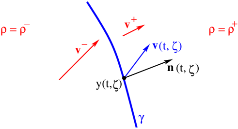
Figure 1: The variables in the equations (2.4), (2.6), determining the evolution of a singular curve $\gamma$.

Calling ${\bf n}(t,\zeta)$ the unit normal vector to the curve at the point $y(t,\zeta)$, as in Fig. 1, we assume that the inner products satisfy the admissibility condition

$$\Big{\langle}{\bf n}(t,\zeta),\,{\bf v}^{+}(t,y(t,\zeta))\Big{\rangle}~{}\leq~{}\Big{\langle}{\bf n}(t,\zeta),\,{\bf v}(t,\zeta)\Big{\rangle}~{}\leq~{}\Big{\langle}{\bf n}(t,\zeta),\,{\bf v}^{-}(t,y(t,\zeta))\Big{\rangle}.$$ (2.3)

These inequalities imply that particles impinge on the singular curve from both sides (and then stick to it).

It will be convenient to write the next equation using the cross product of two vectors ${\bf u}=(u_{1},u_{2})$, ${\bf v}=(v_{1},v_{2})$ in ${\mathbb{R}}^{2}$:

$${\bf u}\times{\bf v}~{}=~{}u_{1}v_{2}-u_{2}v_{1}~{}=~{}\big{\langle}{\bf u}^{\perp},{\bf v}\big{\rangle},\qquad{\bf u}^{\perp}=(-u_{2},u_{1}).$$

Under the assumption (2.3), for any $\zeta_{1}<\zeta_{2}$ the rate at which the mass along the curve increases is computed by

$${d\over dt}\int_{\zeta_{1}}^{\zeta_{2}}\eta(t,\zeta)\,d\zeta~{}=~{}\int_{\zeta_{1}}^{\zeta_{2}}\rho^{+}({\bf v}-{\bf v}^{+})\times y_{\zeta}\,d\zeta+\int_{\zeta_{1}}^{\zeta_{2}}\rho^{-}({\bf v}^{-}-{\bf v})\times y_{\zeta}\,d\zeta\,.$$

Since the above identity holds for all $\zeta_{1}<\zeta_{2}$, this implies

$$\eta_{t}(t,\zeta)~{}=~{}\rho^{+}({\bf v}-{\bf v}^{+})\times y_{\zeta}+\rho^{-}({\bf v}^{-}-{\bf v})\times y_{\zeta}\,,$$ (2.4)

where the functions $\rho^{\pm},{\bf v}^{\pm}$ are evaluated at $(t,y(t,\zeta))$.

A similar argument shows that, by conservation of momentum, one has

$$\bigl{[}\eta(t,\zeta)\,{\bf v}(t,\zeta)\bigr{]}_{t}~{}=~{}[({\bf v}-{\bf v}^{+})\times y_{\zeta}]\,\rho^{+}{\bf v}^{+}+[({\bf v}^{-}-{\bf v})\times y_{\zeta}]\,\rho^{-}{\bf v}^{-}.$$ (2.5)

Combining (2.4) with (2.5), one obtains an expression for ${\bf v}_{t}(t,\zeta)$, describing the acceleration of a particle along the singular curve.

$$\begin{array}[]{rl}\displaystyle y_{tt}(t,\zeta)&=~{}{\bf v}_{t}(t,\zeta)~{}\displaystyle=~{}\left({\eta{\bf v}\over\eta}\right)_{t}~{}=~{}{(\eta{\bf v})_{t}\over\eta}-{\eta_{t}\over\eta}\,{\bf v}\\[11.38109pt] &\displaystyle=~{}{1\over\eta}\bigg{(}\bigl{[}({\bf v}-{\bf v}^{+})\times y_{\zeta}\bigr{]}\,\rho^{+}({\bf v}^{+}-{\bf v})+\bigl{[}({\bf v}^{-}-{\bf v})\times y_{\zeta}\bigr{]}\,\rho^{-}({\bf v}^{-}-{\bf v})\bigg{)}.\end{array}$$ (2.6)

For analytic initial data

$$y(t_{0},\zeta)\,=\,y_{0}(\zeta),\qquad\eta(t_{0},\zeta)\,=\,\eta_{0}(\zeta),\qquad{\bf v}(t_{0},\zeta)\,=\,{\bf v}_{0}(\zeta),$$ (2.7)

a local solution to the Cauchy problem (2.4), (2.6), (2.7) was constructed in [7] by an application of the classical Cauchy-Kovalevskaya theorem [19, 27, 32].

In the setting considered earlier in [7], the singular curve has already been formed. Namely, $\eta_{0}(\zeta)>0$, while $\rho^{+},\rho^{-}$ are bounded analytic functions. The present situation requires a more careful analysis. Indeed, $\eta_{0}(\zeta_{0})=0$, while $\rho^{-},\rho^{+}\to+\infty$ as $(t,x)\to(t_{0},x_{0})$. In (2.6) these unbounded terms must be partially cancelled by the vanishingly small terms ${\bf v}^{\pm}-{\bf v}$, so that the right hand side remains integrable. In Section 5 we will show that this problem can be reformulated as a system of Briot-Bouquet type, to which the result in [26] can be applied.

3 Singularity formation in one space dimension

In the one dimensional case, a singularity consists of a point mass. The formation of a new singularity is similar to the formation of a new shock in the solution to a scalar conservation law. Geometric ideas from [24] can thus be used also in the present situation.

Let $\bar{\rho}(x)$ and $w(x)$ be the initial density and the initial velocity of the pressureless gas, at the point $x\in{\mathbb{R}}$. Assuming $w^{\prime}(x)<0$, the blowup time along the characteristic starting at $x$ is

$$\tau(x)~{}=~{}{-1\over w^{\prime}(x)}\,.$$ (3.1)

We assume that, at a point $x_{0}$, the velocity satisfies

$$w^{\prime}(x_{0})\,=\,-{1\over t_{0}}\,<\,0,\qquad\quad w^{\prime\prime}(x_{0})=0,\quad\qquad w^{\prime\prime\prime}(x_{0})>0\,.$$ (3.2)

As a consequence, $w^{\prime}$ has a negative minimum at $x_{0}$, and hence $t_{0}=\tau(x_{0})$ is a local minimum of the blow-up time function $\tau(\cdot)$. In other words, $t_{0}$ is the first time when the singularity appears.

Without loss of generality, to simplify notation we shall assume that $x_{0}=0$. To fix ideas, let the density and velocity functions have the Taylor approximation

$$\bar{\rho}(x)~{}=~{}\sum_{k\geq 0}\rho_{k}{x^{k}\over k!}\,$$ (3.3)

$$w(x)~{}=~{}\omega_{0}-\omega_{1}x+\sum_{k\geq 3}{\omega_{k}}{x^{k}\over k!}\,,$$ (3.4)

where the coefficients satisfy

$$\rho_{0}>0,\qquad\omega_{1}>0,\qquad\omega_{3}>0.$$ (3.5)

In the above setting, we have

Theorem 3.1

Let the initial density and velocity of the 1-dimensional pressureless gas be analytic functions satisfying (3.3)–(3.5). Then there exists a local solution containing a point mass along an analytic curve $t\mapsto y(t)$, $t\in\,]t_{0},t_{0}+\delta]$. Here $t_{0}=1/\omega_{1}$, $y(t_{0})=t_{0}\omega_{0}$.

Moreover, the mass has asymptotic size $m(t)=\sqrt{t-t_{0}}\cdot\Upsilon(t)$, where $\Upsilon$ is an analytic function with $\Upsilon(t_{0})>0$.

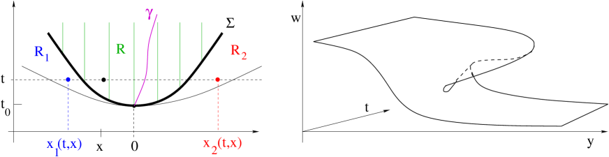
Figure 2: Left: the regions $R,R_{1},R_{2}$ introduced at (3.6)–(3.8). Here $\gamma$ is the stable manifold of the vector field ${\bf f}$ in (3.23) at the equilibrium point $(t_{0},0)$. Right: the image of the map $(t,x)\mapsto(t,y,w)=\bigl{(}t,x+tw(x),w(x)\bigr{)}$. For $t>t_{0}$, this sheet has a fold. Indeed, if $(t,x)\in R$, there are two additional values $x_{1}(t,x)<x<x_{2}(t,x)$ such that (3.9) holds. Here $(t,x_{1})\in R_{1}$ while $(t,x_{2})\in R_{2}$.

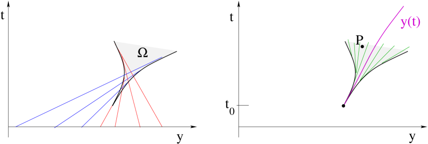
Figure 3: Every point $P=(t,y)$ in the region $\Omega$ defined at (3.10) is reached by three distinct characteristics. Namely, there exist $x_{1}<x<x_{2}$ such that (3.9) holds.

Proof. 1. To construct the singular curve $y(\cdot)$, following [24] we shall use an alternative set of coordinates. As shown in Fig. 2, left, in the $t$-$x$ plane we consider the domain

$$R~{}=~{}\bigl{\{}(t,x)\,;~{}t>\tau(x)\bigr{\}}~{}=~{}\bigl{\{}(t,x);~{}1+tw^{\prime}(x)<0\bigr{\}},$$ (3.6)

with boundary

$$\Sigma~{}=~{}\bigl{\{}(\tau(x),x)\,;~{}x\in{\mathbb{R}}\bigr{\}}\,.$$ (3.7)

For $(t,x)\in R$, there are two additional points $(t,x_{1}(t,x))\in R_{1}$ and $(t,x_{2}(t,x))\in R_{2}$, with

$$x_{1}(t,x)~{}<~{}x~{}<~{}x_{2}(t,x)\,,\qquad\qquad\tau(x_{1})\,>\,t,\quad\tau(x)\,<\,t,\quad\tau(x_{2})\,>\,t,$$ (3.8)

and such that

$$x_{1}+tw(x_{1})~{}=~{}x+tw(x)~{}=~{}x_{2}+tw(x_{2}).$$ (3.9)

In other words, the three characteristics starting at $x$, $x_{1}$ and $x_{2}$ reach exactly the same point $y$ at time $t$. As shown in Figures 2 and 3, there is a cusp region covered by three sheets of the map $(t,x)\mapsto\bigr{(}t,x+tw(x),w(x)\bigl{)}$, namely

$$\Omega~{}=~{}\Big{\{}(t,y)\,;~{}y=x+tw(x),~{}t>\tau(x)\quad\hbox{for some }~{}x\in{\mathbb{R}}\Big{\}}.$$ (3.10)

According to (3.10), we shall parameterize points $(t,y)\in\Omega$ by the pull-back along the characteristic on the middle sheet. 2. As before, we call $y(t)$ and $m(t)$ the position and the amount of mass concentrated at the singular point at time $t>t_{0}$. Writing

$$y(t)~{}=~{}x(t)+tw\bigl{(}x(t)\bigr{)},$$ (3.11)

we seek an evolution equation for $x(\cdot)$ and $m(\cdot)$. Conservation of mass and momentum yield

$$m(t)~{}=~{}\int_{x_{1}(t,x(t))}^{x_{2}(t,x(t))}\bar{\rho}(\xi)\,d\xi,\qquad\qquad m(t)\dot{y}(t)~{}=~{}\int_{x_{1}(t,x(t))}^{x_{2}(t,x(t))}\bar{\rho}(\xi)w(\xi)\,d\xi\,.$$ (3.12)

3. To proceed, we need an efficient representation of the maps $x_{1}(t,x)$, $x_{2}(t,x)$. These provide solutions $X=X(t,x)$ to the scalar equation

$$X+tw(X)~{}=~{}x+tw(x).$$ (3.13)

Consider the analytic function

$$f(X,t,x)~{}\doteq~{}\left\{\begin{array}[]{cl}\displaystyle 1+t\,{w(X)-w(x)\over X-x}&\hbox{if}\quad X\not=x,\\[11.38109pt] 1+t\,w^{\prime}(x)&\hbox{if}\quad X=x.\end{array}\right.$$ (3.14)

Notice that, by replacing the equation (3.13) with

$$f(X,t,x)~{}=~{}0,$$ (3.15)

we can remove the trivial solution $X=x$. In view of (3.4), at $t=t_{0}$ we find

$$f(X,t_{0},0)~{}=~{}g(X)\,X^{2},$$

where $g$ is an analytic function such that $g(0)={t_{0}\,\omega_{3}/6}>0$. According to the Weierstrass Preparation Theorem (see for example [13] or [20]), for $(t,x)\approx(t_{0},0)$ there exists an analytic function $q$, together with analytic functions $a_{1},a_{2}$ such that

$$q(X,t,x)\,f(X,t,x)~{}=~{}X^{2}-2a_{1}(t,x)X+a_{0}(t,x),$$ (3.16)

with

$$a_{0}(t_{0},0)~{}=~{}a_{1}(t_{0},0)~{}=~{}0,\qquad\qquad q(0,t_{0},0)\not=0.$$

Since our goal is to find solutions of (3.15), the above representation clarifies the structure of these solutions. Indeed,

$$\begin{array}[]{l}\displaystyle x_{1}(t,x)~{}=~{}a_{1}(t,x)-\sqrt{a_{1}^{2}(t,x)-a_{0}(t,x)}\,,\\[5.69054pt] \displaystyle x_{2}(t,x)~{}=~{}a_{1}(t,x)+\sqrt{a_{1}^{2}(t,x)-a_{0}(t,x)}\,.\end{array}$$ (3.17)

4. Next, for any smooth function $\phi$ we can write

$$\int_{x-s}^{x+s}\phi(y)\,dy~{}=~{}\Phi(x,s^{2})\,s\,,$$ (3.18)

for a suitable function $\Phi$. Indeed, the left hand side is an odd function of $s$. Hence it can be written as a product of $s$ and an even function of $s$. In connection with (3.12), (3.17), this yields

$$m(t)~{}=~{}\int_{x_{1}(t,x(t))}^{x_{2}(t,x(t))}\bar{\rho}(\xi)\,d\xi~{}=~{}M(t,x)\cdot\sqrt{a_{1}^{2}(t,x)-a_{0}(t,x)},$$ (3.19)

$$m(t)\dot{y}(t)~{}=~{}\int_{x_{1}(t,x(t))}^{x_{2}(t,x(t))}\bar{\rho}(\xi)w(\xi)\,d\xi~{}=~{}G(t,x)\cdot\sqrt{a_{1}^{2}(t,x)-a_{0}(t,x)}\,,$$ (3.20)

for suitable analytic functions $M,G$.

Since

$$M(t_{0},0)~{}=~{}2\bar{\rho}(0)~{}\not=0,\qquad\qquad G(t_{0},0)~{}=~{}2\bar{\rho}(0)\,w(0),$$

the function

$$F(t,x)~{}\doteq~{}{G(t,x)\over M(t,x)}-w(x)$$ (3.21)

is analytic in a neighborhood of $(t_{0},0)$. By (3.19)-(3.20) we have to solve

$$\dot{y}~{}=~{}\dot{x}+w(x)+tw^{\prime}(x)\,\dot{x}~{}=~{}{G(t,x)\over M(t,x)}\,.$$

In view of (3.21), this leads to

$$(1+tw^{\prime}(x))\dot{x}~{}=~{}F(t,x).$$ (3.22)

Observing that

$$1+t_{0}w^{\prime}(0)~{}=~{}0~{}=~{}F(t_{0},0),\qquad\qquad t_{0}\,=\,{-1\over w^{\prime}(0)}\,=\,{1\over\omega_{1}}\,,$$

a solution to (3.22) can be constructed by finding an integral curve $\gamma$ of the vector field with analytic components

$${\bf f}~{}=~{}\Big{(}1+tw^{\prime}(x)\,,~{}F(t,x)\Big{)}$$ (3.23)

that goes through the equilibrium point $(t_{0},0)$. We claim that this equilibrium is a saddle.

Indeed, at the point $(t,x)=(t_{0},0)$ the Jacobian matrix has the form

$$D{\bf f}(t_{0},0)~{}=~{}\begin{pmatrix}-\omega_{1}&&&0\\[5.69054pt] \displaystyle{3\omega_{1}^{3}\omega_{4}\over 4\omega_{3}^{2}}-{2\rho_{1}\omega_{1}^{3}\over\rho_{0}\omega_{3}}&&&\displaystyle{3\over 2}\omega_{1}\end{pmatrix}.$$ (3.24)

This claim will be proved in Lemma 3.1 below. 5. Assuming that (3.24) holds, we can proceed with the proof of the theorem. Consider the stable manifold for the vector field (3.23) through the equilibrium point $(t_{0},0)$. Calling $t\mapsto x(t)$ the portion of this manifold for $t>t_{0}$, we obtain the desired integral curve of ${\bf f}$ through $(t_{0},0)$. In turn, the formula (3.11) yields the position of the singularity $y(t)$. We observe that, since the functions $\bar{\rho},w$ are analytic, the stable manifold is analytic as well. See [31] for a general result in this direction.

Finally, the amount of mass concentrated at $y(t)$ is computed by (3.12). More precisely, recalling (3.3), by (3.12) and (3.17) one obtains

$$\begin{array}[]{rl}m(t)&\displaystyle=~{}\sum_{k=0}^{\infty}\int_{a_{1}(t,x(t))-\sqrt{a_{1}^{2}(t,x(t))-a_{0}(t,x(t))}}^{a_{1}(t,x(t))+\sqrt{a_{1}^{2}(t,x(t))-a_{0}(t,x(t))}}{\rho_{k}x^{k}\over k!}\,dx\\[11.38109pt] &=~{}\displaystyle\sum_{k=0}^{\infty}{\rho_{k}\over(k+1)!}\left[\sum_{0\leq j\leq k+1\atop j~{}{\rm odd}}2\Big{(}\begin{matrix}j\cr k+1\end{matrix}\Big{)}\big{(}a_{1}^{2}(t,x(t))-a_{0}(t,x(t))\bigr{)}^{j/2}\cdot a_{1}(t,x(t))^{k+1-j}\right]\\[11.38109pt] &=~{}\sqrt{a_{1}^{2}(t,x(t))-a_{0}(t,x(t))}\cdot\widetilde{\Upsilon}(t)\\[11.38109pt] &=~{}\sqrt{t-t_{0}}\cdot\Upsilon(t),\end{array}$$ (3.25)

where $\widetilde{\Upsilon},\Upsilon$ are analytic functions. This completes the proof. MM     

Lemma 3.1

Assume that the functions $\bar{\rho},w$ have the Taylor approximations (3.3)-(3.4). Then, at the equilibrium point $(t_{0},0)$ the Jacobian matrix of ${\bf f}$ is given by (3.24).

Proof. 1. To compute the partial derivatives of $F$, we begin by observing that, by (3.4), the equation (3.13) can be written as

$$(X-x)+t\left(-\omega_{1}(X-x)+\sum_{k\geq 3}\omega_{k}{X^{k}-x^{k}\over k!}\right)~{}=~{}0.$$ (3.26)

Dividing by $X-x$ we remove the trivial solution $X=x$. The remaining two solutions are found by solving

$$1-t\omega_{1}+t\sum_{k\geq 3}{\omega_{k}\over k!}\left(\sum_{j=0}^{k-1}X^{j}x^{k-1-j}\right)~{}=~{}0.$$ (3.27)

Collecting lower order terms and recalling that $t_{0}\omega_{1}=1$, we obtain

$$-\omega_{1}(t-t_{0})+{t\omega_{3}\over 6}\bigl{(}X^{2}+Xx+x^{2}\bigr{)}+{t\omega_{4}\over 24}\bigl{(}X^{3}+X^{2}x+Xx^{2}+x^{3}\bigr{)}+t\,\Psi(X,x)~{}=~{}0,$$ (3.28)

where $\Psi$ is an analytic function such that

$$\Psi(X,x)~{}=~{}{\cal O}(1)\cdot\bigl{(}|X|^{4}+|x|^{4}\bigr{)}.$$ (3.29)

Dividing all terms by $t\omega_{3}/6$ and recalling that $t_{0}\omega_{1}=1$, we are led to the equation

$$f(X,t,x)~{}\doteq~{}X^{2}+xX+x^{2}-{6\omega_{1}(t-t_{0})\over t\omega_{3}}+{\omega_{4}\over 4\omega_{3}}(X^{3}+X^{2}x+Xx^{2}+x^{3})+{6\Psi(X,x)\over\omega_{3}}~{}=~{}0\,.$$ (3.30)

Assuming $x={\cal O}(1)\cdot(t-t_{0})$, to leading order the solution is given by

$$X^{\pm}(t,x)~{}=~{}\pm\sqrt{{6\omega_{1}(t-t_{0})\over t\omega_{3}}}+{\cal O}(1)\cdot(t-t_{0})\,.$$ (3.31)

Observing that

$$(X^{\pm})^{3}~{}=~{}\pm\left({6\omega_{1}(t-t_{0})\over t\omega_{3}}\right)^{3/2}+{\cal O}(1)\cdot(t-t_{0})^{2}$$

and inserting this expression in (3.30), to the next order one finds

$$\begin{array}[]{rl}X^{\pm}(t,x)&\approx\,\displaystyle-{x\over 2}\pm\sqrt{{6\omega_{1}(t-t_{0})\over t\omega_{3}}\mp{\omega_{4}\over 4\omega_{3}}\left({6\omega_{1}(t-t_{0})\over t\omega_{3}}\right)^{3/2}}+{\cal O}(1)\cdot(t-t_{0})^{3/2}\\[11.38109pt] &\displaystyle=\,-{x\over 2}\pm\sqrt{{6\omega_{1}(t-t_{0})\over t\omega_{3}}}\cdot\sqrt{1\mp{\omega_{4}\over 4\omega_{3}}\left({6\omega_{1}(t-t_{0})\over t\omega_{3}}\right)^{1/2}}+{\cal O}(1)\cdot(t-t_{0})^{3/2}\\[11.38109pt] &\displaystyle=\,-{x\over 2}\pm\sqrt{{6\omega_{1}(t-t_{0})\over t\omega_{3}}}-{3\omega_{1}\omega_{4}(t-t_{0})\over 4t\omega^{2}_{3}}+{\cal O}(1)\cdot(t-t_{0})^{3/2}\\[11.38109pt] &\displaystyle=\,-{x\over 2}\pm\sqrt{{6\omega_{1}^{2}(t-t_{0})\over\omega_{3}}}-{3\omega_{1}^{2}\omega_{4}(t-t_{0})\over 4\omega^{2}_{3}}+{\cal O}(1)\cdot(t-t_{0})^{3/2}\\[11.38109pt] &=\displaystyle~{}\pm B-C+{\cal O}(1)\cdot(t-t_{0})^{3/2},\end{array}$$ (3.32)

where we set

$$B~{}\doteq~{}\sqrt{{6\omega_{1}^{2}(t-t_{0})\over\omega_{3}}},\qquad\qquad C~{}\doteq~{}{x\over 2}+{3\omega_{1}^{2}\omega_{4}(t-t_{0})\over 4\omega_{3}^{2}}\,.$$ (3.33)

2. Computing a Taylor expansion of the integrand in (3.19), for some analytic function $R_{4}(\cdot)$ by (3.3) we obtain

$$\begin{array}[]{rl}m(t)&\displaystyle=~{}\bigg{[}\rho_{0}x+\rho_{1}{x^{2}\over 2}+\rho_{2}{x^{3}\over 3!}+R_{4}(x)x^{4}\bigg{]}_{X^{-}}^{X^{+}}\\[11.38109pt] &\displaystyle=~{}2\rho_{0}B-2\rho_{1}BC+{\rho_{2}\over 3}B^{3}+{\cal O}(1)\cdot(t-t_{0})^{2},\end{array}$$ (3.34)

A similar expansion holds for (3.20). Recalling (3.4), for some analytic function $W_{4}(\cdot)$ we find

$$\begin{array}[]{rl}m(t)\dot{y}(t)&\displaystyle=~{}\bigg{[}\rho_{0}\omega_{0}x+(\rho_{1}\omega_{0}-\rho_{0}\omega_{1}){x^{2}\over 2}+(\rho_{2}\omega_{0}-2\rho_{1}\omega_{1}){x^{3}\over 6}+W_{4}(x)x^{4}\bigg{]}_{X^{-}}^{X^{+}}\\[11.38109pt] &\displaystyle=~{}2\rho_{0}\omega_{0}B-2(\rho_{1}\omega_{0}-\rho_{0}\omega_{1})BC+{\rho_{2}\omega_{0}-2\rho_{1}\omega_{1}\over 3}B^{3}+{\cal O}(1)\cdot(t-t_{0})^{2}.\end{array}$$ (3.35)

Combining (3.34), (3.35) and recalling (3.21) we finally obtain

$$\begin{array}[]{rl}F(t,x)&\displaystyle=~{}{2\rho_{0}\omega_{0}B-2(\rho_{1}\omega_{0}-\rho_{0}\omega_{1})BC+(\rho_{2}\omega_{0}-2\rho_{1}\omega_{1})(B^{3}/3)\over 2\rho_{0}B-2\rho_{1}BC+\rho_{2}(B^{3}/3)}-\omega_{0}+\omega_{1}x+{\cal O}(1)\cdot(t-t_{0})^{3/2}\\[11.38109pt] &\displaystyle=~{}{\displaystyle\omega_{0}-{\rho_{1}\omega_{0}-\rho_{0}\omega_{1}\over\rho_{0}}C+{\rho_{2}\omega_{0}-2\rho_{1}\omega_{1}\over 6\rho_{0}}B^{2}\over\displaystyle 1-{\rho_{1}\over\rho_{0}}C+{\rho_{2}\over 6\rho_{0}}B^{2}}-\omega_{0}+\omega_{1}x+{\cal O}(1)\cdot(t-t_{0})^{3/2}\\[11.38109pt] &=~{}\displaystyle\left(\omega_{0}-{\rho_{1}\omega_{0}-\rho_{0}\omega_{1}\over\rho_{0}}C+{\rho_{2}\omega_{0}-2\rho_{1}\omega_{1}\over 6\rho_{0}}B^{2}\right)\left(1+{\rho_{1}\over\rho_{0}}C-{\rho_{2}\over 6\rho_{0}}B^{2}\right)\\[11.38109pt] &\qquad-\omega_{0}+\omega_{1}x+{\cal O}(1)\cdot(t-t_{0})^{3/2}\\[11.38109pt] &=~{}\displaystyle\omega_{1}C-{\rho_{1}\omega_{1}\over 3\rho_{0}}B^{2}+\omega_{1}x+{\cal O}(1)\cdot(t-t_{0})^{3/2}.\end{array}$$ (3.36)

By (3.33), this yields

$$\begin{array}[]{rl}F(t,x)&\displaystyle=~{}\omega_{1}\left({x\over 2}+{3\omega_{1}^{2}\omega_{4}(t-t_{0})\over 4\omega_{3}^{2}}\right)-{\rho_{1}\omega_{1}\over 3\rho_{0}}\left({6\omega_{1}^{2}(t-t_{0})\over\omega_{3}}\right)+\omega_{1}x+{\cal O}(1)\cdot(t-t_{0})^{3/2}\\[11.38109pt] &\displaystyle=~{}\left({3\omega_{1}^{3}\omega_{4}\over 4\omega_{3}^{2}}-{2\rho_{1}\omega_{1}^{2}\over\rho_{0}\omega_{3}}\right)(t-t_{0})+{3\over 2}\omega_{1}x+{\cal O}(1)\cdot(t-t_{0})^{3/2}.\end{array}$$ (3.37)

In view of (3.37), since $w^{\prime\prime}(0)=0$, the partial derivatives of the vector field ${\bf f}$ in (3.23) at the point $(t_{0},0)$ are now computed according to (3.24). MM     

Remark 3.1

In view of (3.24), at the equilibrium point $(t_{0},0)$ the first eigenvalue and eigenvector of the matrix $D{\bf f}$ are computed by

$$\lambda_{1}\,=\,-\omega_{1},\qquad\qquad{\bf w}_{1}~{}=~{}\left(\begin{array}[]{c}1\cr S_{0}\end{array}\right),\qquad S_{0}~{}=~{}{2\over 5\omega_{1}}\left({2\rho_{1}\omega_{1}^{3}\over\rho_{0}\omega_{3}}-{3\omega_{1}^{3}\omega_{4}\over 4\omega_{3}^{2}}\right).$$ (3.38)

The second pair is

$$\lambda_{2}~{}=~{}{3\over 2}\omega_{1}\,,\qquad\qquad{\bf w}_{2}~{}=~{}\left(\begin{array}[]{c}0\cr 1\end{array}\right).$$ (3.39)

Recalling that $\omega_{1}>0$, we conclude that the stable manifold $t\mapsto x(t)$ has asymptotic expansion

$$x(t)~{}=~{}S_{0}(t-t_{0})+{\cal O}(1)\cdot(t-t_{0})^{2},\qquad\qquad S_{0}\,=\,{4\over 5}\,{\rho_{1}\omega_{1}^{2}\over\rho_{0}\omega_{3}}-{3\over 10}\,{\omega_{1}^{2}\omega_{4}\over\omega_{3}^{2}}.$$ (3.40)

3.1 The second order system.

In one space dimension, the conservation of mass and momentum yield the identities (3.12). However, similar identities are not available in dimension $n\geq 2$. As a preliminary to the analysis of the 2-dimensional case, we study here the corresponding second order system of equations. Denoting derivatives w.r.t. time with an upper dot, these take the form

$$\left\{\begin{array}[]{rl}\dot{m}&=~{}(v^{-}-v)\rho^{-}-(v^{+}-v)\rho^{+},\\[2.84526pt] \dot{y}&=~{}v,\\[2.84526pt] \dot{v}&=~{}\displaystyle{\rho^{-}\over m}(v^{-}-v)^{2}-{\rho^{+}\over m}(v^{+}-v)^{2}.\end{array}\right.$$ (3.41)

The initial data at $t=t_{0}$ are

$$\left\{\begin{array}[]{rl}m(t_{0})&=~{}0,\\[2.84526pt] y(t_{0})&=~{}x_{0}+t_{0}\,w(x_{0}),\\[2.84526pt] v(t_{0})&=~{}w(x_{0}).\end{array}\right.$$ (3.42)

Differentiating w.r.t. time the identity

$$y~{}=~{}x+tw(x),$$ (3.43)

one finds

$$\dot{y}~{}=~{}w(x)+\bigl{[}1+tw^{\prime}(x)\bigr{]}\dot{x},$$ (3.44)

$$\ddot{y}~{}=~{}\bigl{[}1+tw^{\prime}(x)\bigr{]}\ddot{x}+2w^{\prime}(x)\dot{x}+t\,w^{\prime\prime}(x)\dot{x}^{2}.$$ (3.45)

In the following, we denote the density and speed behind and ahead of the singularity as functions of the variables $t,x$, namely

$$\rho^{\pm}(t,x)~{}=~{}\bigl{[}1+tw^{\prime}\bigl{(}X^{\pm}(t,x)\bigr{)}\bigr{]}^{-1}\bar{\rho}\bigl{(}X^{\pm}(t,x)\bigr{)},\qquad\qquad v^{-}(t,x)~{}=~{}w\bigl{(}X^{-}(t,x)\bigr{)}.$$ (3.46)

where $X^{+},X^{-}$ are the two solutions of (3.26), computed at (3.32)-(3.33).

Setting $S=\dot{x}$, in these new variables the system (3.41) takes the form

$$\left\{\begin{array}[]{rl}\dot{m}&=~{}\displaystyle\Big{(}w(x)+\bigl{[}1+tw^{\prime}(x)\bigr{]}S-v^{+}\Big{)}\rho^{+}-\Big{(}w(x)+\bigl{[}1+tw^{\prime}(x)\bigr{]}S-v^{-}\Big{)}\,\rho^{-},\\[11.38109pt] \dot{x}&=~{}S,\\[8.53581pt] \dot{S}&=~{}\displaystyle\bigl{[}1+tw^{\prime}(x)\bigr{]}^{-1}\Bigg{\{}\Big{(}w(x)+\bigl{[}1+tw^{\prime}(x)\bigr{]}S-v^{-}\Big{)}^{2}{\rho^{-}\over m}\\[11.38109pt] &\qquad\qquad\displaystyle-\Big{(}w(x)+\bigl{[}1+tw^{\prime}(x)\bigr{]}S-v^{+}\Big{)}^{2}{\rho^{+}\over m}-2w^{\prime}(x)S-t\,w^{\prime\prime}(x)S^{2}\Bigg{\}}.\end{array}\right.$$ (3.47)

Of course, the solution to (3.47) is the same one described in Theorem 3.1. Toward a future extension to the 2-dimensional case we remark that, while (3.47) contains three equations, only two initial conditions are given, namely

$$m(t_{0})=0,\qquad\qquad x(t_{0})=0.$$ (3.48)

At this stage, an important observation is that the initial value $S_{0}=\dot{x}(t_{0})$ can be uniquely determined by imposing the integrability of the right hand side of the last equation in (3.47). Indeed, the map $t\mapsto\bigl{[}1+tw^{\prime}(x)\bigr{]}^{-1}$ is not integrable in a neighborhood of $t=t_{0}$. To achieve a well defined solution it is essential that, on the right hand side of this equation, the second factor within brackets vanishes at $t=t_{0}$.

Assume that

$$x(t)~{}=~{}S_{0}(t-t_{0})+{\cal O}(1)\cdot(t-t_{0})^{2},$$ (3.49)

for some constant $S_{0}$ to be determined. By (3.32) this implies

$$X^{\pm}(t)~{}=~{}-{S_{0}(t-t_{0})\over 2}\pm\sqrt{{6\omega_{1}^{2}(t-t_{0})\over\omega_{3}}}-{3\omega_{1}^{2}\omega_{4}(t-t_{0})\over 4\omega^{2}_{3}}+{\cal O}(1)\cdot(t-t_{0})^{3/2}.$$ (3.50)

Recalling that $\omega_{1}t_{0}=1$, from (3.3)-(3.4) we obtain

$$1+tw^{\prime}\bigl{(}x(t)\bigr{)}~{}=~{}-\omega_{1}(t-t_{0})+{\cal O}(1)\cdot(t-t_{0})^{2},$$ (3.51)

$$v^{-}-v^{+}~{}=~{}w\bigl{(}X^{-}(t)\bigr{)}-w\bigl{(}X^{+}(t)\bigr{)}~{}=~{}2\omega_{1}\sqrt{6\omega_{1}^{2}(t-t_{0})\over\omega_{3}}+{\cal O}(1)\cdot(t-t_{0}).$$

$$v^{-}-w(x)~{}=~{}\omega_{1}^{2}\sqrt{6(t-t_{0})\over\omega_{3}}+{\cal O}(1)\cdot(t-t_{0}).\,,$$

In addition, by (3.50) we have the leading order approximations

$$\begin{array}[]{rl}1+tw^{\prime}(X^{\pm})&\displaystyle=\,-\omega_{1}(t-t_{0})+t_{0}\omega_{3}{(X^{\pm})^{2}\over 2}+t_{0}\omega_{4}{(X^{\pm})^{3}\over 6}+{\cal O}(1)\cdot(t-t_{0})^{2}\\[11.38109pt] &=~{}2\omega_{1}(t-t_{0})\bigl{(}1\mp E\cdot\sqrt{t-t_{0}}\,\bigr{)}+{\cal O}(1)\cdot(t-t_{0})^{2}\,,\end{array}$$ (3.52)

where

$$E\,\doteq\,\frac{\omega_{3}^{2}S_{0}-\frac{1}{2}\omega_{1}^{2}\omega_{4}}{4\omega_{1}\omega_{3}}\sqrt{\frac{6}{\omega_{3}}}.$$ (3.53)

In turn, this yields

$$\rho^{\pm}~{}=~{}\frac{\bar{\rho}(X^{\pm})}{1+tw^{\prime}(X^{\pm})}~{}=~{}\frac{1}{2\omega_{1}(t-t_{0})}\left[\rho_{0}\pm\left(\rho_{1}\omega_{1}\sqrt{\frac{6}{\omega_{3}}}+\rho_{0}E\right)\sqrt{t-t_{0}}\right]+{\cal O}(1),$$ (3.54)

$$\dot{m}~{}=~{}(v^{-}-v^{+})\rho^{+}+\Big{(}w(x)+\bigl{[}1+tw^{\prime}(x)\bigr{]}S-v^{-}\Big{)}\,(\rho^{+}-\rho^{-})~{}=\displaystyle~{}{\omega_{1}\rho_{0}\over\sqrt{t-t_{0}}}\,\sqrt{6\over\omega_{3}}+{\cal O}(1)\,,$$

$$m(t)~{}=~{}2\omega_{1}\rho_{0}\sqrt{6(t-t_{0})\over\omega_{3}}+{\cal O}(1)\cdot(t-t_{0}).$$ (3.55)

In particular, on the right hand side of (3.47), the coefficients of the terms containing $S^{2}=\dot{x}^{2}$ have size

$$\left\{\begin{array}[]{rl}\displaystyle\bigl{[}1+tw^{\prime}(x)\bigr{]}^{2}{\rho^{-}-\rho^{+}\over m}&\displaystyle=~{}{\cal O}(1)\cdot(t-t_{0})^{2}\cdot{(t-t_{0})^{-1/2}\over(t-t_{0})^{1/2}}~{}=~{}{\cal O}(1)\cdot(t-t_{0}),\\[11.38109pt] tw^{\prime\prime}(x)&=~{}{\cal O}(1)\cdot(t-t_{0}).\end{array}\right.$$ (3.56)

Therefore, even after multiplication by $\bigl{[}1+tw^{\prime}(x)\bigr{]}^{-1}={\cal O}(1)\cdot(t-t_{0})^{-1}$, these terms are integrable. Thanks to this observation, the integrability of the right hand side in the last equation of (3.47) yields an equation which is linear in $S_{0}$. Recalling that $x(t)\approx(t-t_{0})S_{0}$, we compute the approximations

$$\begin{array}[]{rl}\dot{S}&\displaystyle\approx~{}{-1\over\omega_{1}(t-t_{0})}\cdot\bigg{\{}\Big{(}\omega_{0}-\omega_{1}x(t)-\omega_{1}(t-t_{0})S_{0}-w\bigl{(}X^{-}(t)\bigr{)}\Big{)}^{2}{\rho^{-}(t)\over m(t)}\\[11.38109pt] &\qquad\qquad\qquad\displaystyle-\Big{(}\omega_{0}-\omega_{1}x(t)-\omega_{1}(t-t_{0})S_{0}-w\bigl{(}X^{+}(t)\bigr{)}\Big{)}^{2}{\rho^{+}(t)\over m(t)}+2\omega_{1}S_{0}\bigg{\}}\\[14.22636pt] &\displaystyle\approx~{}{-1\over\omega_{1}(t-t_{0})}\cdot\bigg{\{}\omega_{1}^{2}\bigl{(}X^{-}(t)\bigr{)}^{2}{\rho^{-}(t)\over m(t)}-\omega_{1}^{2}\bigl{(}X^{+}(t)\bigr{)}^{2}{\rho^{+}(t)\over m(t)}\\[11.38109pt] &\qquad\qquad\qquad\displaystyle-\omega_{1}^{2}\frac{4S_{0}(t-t_{0})}{m(t)}\Big{(}\rho^{-}(t)X^{-}(t)-\rho^{+}(t)X^{+}(t)\Big{)}+2\omega_{1}S_{0}\bigg{\}}\\[14.22636pt] &\displaystyle=~{}{-1\over t-t_{0}}\cdot\Bigg{\{}{\omega_{1}\over m(t)}\bigg{(}(X^{-})^{2}\bigl{[}\rho^{-}-\rho^{+}\bigr{]}+\bigl{[}(X^{-})^{2}-(X^{+})^{2}\bigr{]}\rho^{+}\\[11.38109pt] &\qquad\qquad\qquad\qquad\displaystyle-4S_{0}(t-t_{0})\big{(}\rho^{-}X^{-}-\rho^{+}X^{+}\big{)}\bigg{)}+2S_{0}\Bigg{\}}\,.\end{array}$$ (3.57)

We need to impose that the factor within braces vanishes as $t\to t_{0}$. Recalling (3.52) and (3.54), and then using (3.50), we find

$$\begin{array}[]{l}\displaystyle{\omega_{1}\over m(t)}\Big{(}(X^{-})^{2}\bigl{[}\rho^{-}-\rho^{+}\bigr{]}+\bigl{[}(X^{-})^{2}-(X^{+})^{2}\bigr{]}\rho^{+}{-4S_{0}(t-t_{0})\big{(}\rho^{-}X^{-}-\rho^{+}X^{+}\big{)}}\Big{)}+2S_{0}\\[11.38109pt] \displaystyle\qquad\approx{\omega_{1}\over m(t)}\Bigg{\{}-\frac{6\omega_{1}^{2}}{\omega_{3}}(t-t_{0})\cdot\left(\rho_{1}\sqrt{\frac{6}{\omega_{3}}}+\frac{\rho_{0}}{\omega_{1}}E\right){1\over\sqrt{t-t_{0}}}\\[11.38109pt] \displaystyle\qquad\qquad+\frac{2S_{0}\omega_{3}^{2}+3\omega_{1}^{2}\omega_{4}}{\omega_{3}^{2}}\omega_{1}\sqrt{\frac{6}{\omega_{3}}}(t-t_{0})^{3/2}\cdot\frac{1}{2\omega_{1}(t-t_{0})}\left[\rho_{0}+\left(\rho_{1}\omega_{1}\sqrt{\frac{6}{\omega_{3}}}+\rho_{0}E\right)\sqrt{t-t_{0}}\right]\\[11.38109pt] \displaystyle\qquad\qquad-4S_{0}(t-t_{0})\cdot\left({-\rho_{0}\over 2\omega_{1}(t-t_{0})}2\omega_{1}\sqrt{6(t-t_{0})\over\omega_{3}}\,\right)\Bigg{\}}+2S_{0}\,.\end{array}$$ (3.58)

Finally, recalling the expressions for $m(t)$ at (3.55) and for $E$ at (3.53), imposing that the quantity in (3.58) approaches zero as $t\to t_{0}$, we obtain

$$\begin{array}[]{l}\displaystyle 0~{}=~{}{\omega_{1}\over 2\rho_{0}\omega_{1}\sqrt{6/\omega_{3}}}\left\{-\frac{6\omega_{1}^{2}}{\omega_{3}}\cdot\left(\rho_{1}\sqrt{\frac{6}{\omega_{3}}}+\frac{\rho_{0}}{\omega_{1}}E\right)+\frac{2S_{0}\omega_{3}^{2}+3\omega_{1}^{2}\omega_{4}}{\omega_{3}^{2}}\sqrt{\frac{6}{\omega_{3}}}\cdot\frac{\rho_{0}}{2}+4S_{0}\rho_{0}\sqrt{\frac{6}{\omega_{3}}}\;\right\}+2S_{0}\\[14.22636pt] \displaystyle\quad=~{}{1\over 2\rho_{0}}\left\{-\frac{6\omega_{1}^{2}}{\omega_{3}}\cdot\left(\rho_{1}+\frac{\rho_{0}}{\omega_{1}}\cdot\frac{\omega_{3}^{2}S_{0}-\frac{1}{2}\omega_{1}^{2}\omega_{4}}{4\omega_{1}\omega_{3}}\right){+\frac{2S_{0}\omega_{3}^{2}+3\omega_{1}^{2}\omega_{4}}{\omega_{3}^{2}}\cdot\frac{\rho_{0}}{2}}+4S_{0}\rho_{0}\;\right\}+2S_{0}\\[14.22636pt] \displaystyle\quad=~{}\frac{1}{2\rho_{0}}\left(\frac{7}{2}S_{0}\rho_{0}-6\frac{\omega_{1}^{2}\rho_{1}}{\omega_{3}}+\frac{9}{4}\cdot\frac{\rho_{0}\omega_{1}^{2}\omega_{4}}{\omega_{3}^{2}}\right)+2S_{0}\,.\end{array}$$ (3.59)

This yields

$$S_{0}~{}=~{}{4\over 5}{\rho_{1}\omega_{1}^{2}\over\rho_{0}\omega_{3}}-{3\over 10}{\omega_{1}^{2}\omega_{4}\over\omega_{3}^{2}}\,.$$ (3.60)

Notice that, by this different approach, we again recover the same value for $S_{0}$ as in (3.40).

4 Singularity formation in 2D

Beginning with this section, we study the formation of a new singularity in two space dimensions. Assuming that the initial data $\bar{\rho},{\bf w}$ in (1.2) are analytic, we wish to construct a solution of (1.1) beyond the time $t_{0}$ when the singularity first appears. Referring to Fig. 5, for $t>t_{0}$ we expect that the solution will be smooth outside a singular curve $\gamma^{t}$, where a positive amount of mass is concentrated. Outside $\gamma^{t}$, the velocity and the density of the pressureless gas are still computed by (1.3) and (1.4) respectively. To completely describe this solution, it thus remains to determine the position of the singular curve $\gamma^{t}$, and the velocity and density of particles along this curve.

We observe that, in a neighborhood of a point $Q$ in the relative interior of $\gamma^{t}$, where the density $\eta$ is strictly positive, the singular curve is described by the system of equations (2.4)–(2.6). Its local construction has already been worked out in [7]. Aim of this and the next section is to construct the singular curve $\gamma^{t}$ in a neighborhood of an endpoint $P$. The same construction remains valid near the point $P_{0}$ where the singularity first appears.

While the density $\eta$ and the velocity ${\bf v}$ of particles along the singular curve are still determined by the balance of mass and momentum (2.4)-(2.5), we can no longer rely on the 1-dimensional formulas (3.12). Always referring to Fig. 5, near an endpoint $P\in\gamma^{t}\cap\gamma^{\sharp}$, one has

$$\rho^{\pm}\to+\infty,\qquad\qquad\eta\to 0.$$

Therefore, both equations (2.4) and (2.6) contain unbounded terms. Toward the analysis of these two equations, the key step is to get a manageable expression for the functions ${\bf v}^{\pm}$, $\rho^{\pm}$, measuring the velocity and the density of the gas in a neighborhood of the singular curve. Of course, $\rho$ and ${\bf v}$ can be determined a priori, in terms of (1.3)-(1.4). However, in the region where the singular curve is located, every point $(t,y)$ can be reached by three distinct characteristics:

$$y~{}=~{}X_{1}+t{\bf w}(X_{1})~{}=~{}X_{2}+t{\bf w}(X_{2})~{}=~{}X_{3}+t{\bf w}(X_{3}).$$

The points $X_{1},X_{2},X_{3}\in{\mathbb{R}}^{2}$ are thus obtained as the roots of a cubic-like equation. This would lead to very messy computations. In alternative, following the approach used in Section 3 for the 1-dimensional problem, we use one of these solutions as independent coordinates $(t,x)$, and denote by $X_{1}(t,x)$, $X_{2}(t,x)$ the two remaining solutions of

$$X+t{\bf w}(X)~{}=~{}x+t{\bf w}(x).$$

By doing so, the functions $X_{1},X_{2}$ are obtained by solving an equation of quadratic type, and can be conveniently expressed in terms of square roots. As in [24], here $x$ is the initial point of the characteristic reaching $y=x+t{\bf w}(x)$ along the “middle sheet”. It can be distinguished from the other two characteristics by the relations

$$\tau(X_{1})>t,\qquad\tau(x)<t,\qquad\tau(X_{2})>t.$$

Here and in the sequel, $\tau(x)$ denotes the first time $t>0$ where the matrix $I+tD{\bf w}(x)$ is not invertible.

Ultimately, the goal of this section is to obtain a local asymptotic expansion for the velocity and the density of the gas:

$${\bf v}^{-}(t,x)~{}=~{}{\bf w}\bigl{(}X_{1}(t,x)\bigr{)},\qquad{\bf v}^{+}(t,x)~{}=~{}{\bf w}\bigl{(}X_{2}(t,x)\bigr{)},$$

$$\rho^{-}(t,x)~{}=~{}{\bar{\rho}\bigl{(}X_{1}(t,x)\bigr{)}\over\det\bigl{(}I+tD{\bf w}(X_{1}(t,x))\bigr{)}}\,,\qquad\rho^{+}(t,x)~{}=~{}{\bar{\rho}\bigl{(}X_{2}(t,x)\bigr{)}\over\det\bigl{(}I+tD{\bf w}(X_{2}(t,x))\bigr{)}}\,.$$

This will be achieved in Lemma 4.2.

We now start working out details. Let ${\bf w}$ be a vector field satisfying the assumptions in (A1)-(A2). In particular, the $2\times 2$ Hessian matrix $D^{2}\lambda_{1}(x_{0})$ of second order derivatives of $\lambda_{1}$, computed at $x=x_{0}$, is strictly positive definite. Hence the same is true of the Hessian matrix $D^{2}\tau(x_{0})$.

We denote by $\bigl{\{}r_{1}(x),\,r_{2}(x)\bigr{\}}$ a basis of right eigenvectors of $D{\bf w}(x)$, normalized so that

$$\bigl{|}r_{1}(x)\bigr{|}~{}=~{}\bigl{|}r_{2}(x)\bigr{|}~{}=~{}1.$$ (4.1)

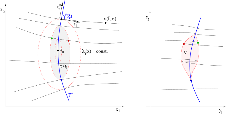
Figure 4: Left: the integral curves of the corresponding eigenvector $r_{1}$, and the level sets of the eigenvalue $\lambda_{1}(x)$ of $D{\bf w}(x)$, which coincide with the level curves of the blow-up time $\tau(x)=-1/\lambda_{1}(x)$. Here $\gamma^{*}$ is the set of points where these two families of curves are tangent. Moreover, $x(\xi,\sigma)$ is the point reached by starting at $\gamma^{*}(\xi)$ and moving along the integral curve of the vector field $r_{1}$ for a time $\sigma$. Right: the shaded region $V$ is the image of the set $\{x;\,\tau(x)<t_{1}\}$, under the map $x\mapsto x+t_{1}{\bf w}(x)$. Each point $y\in V$ has three pre-images.

In the above setting, by the implicit function theorem there exists a smooth curve

$$\gamma^{*}~{}\doteq~{}\Big{\{}x\in{\mathbb{R}}^{2}\,;~{}\big{\langle}\nabla\lambda_{1}(x)\,,\,r_{1}(x)\big{\rangle}\,=\,0\Big{\}},$$ (4.2)

defined near $x_{0}$ (see Fig. 4, left). Indeed, since $\nabla\lambda_{1}(x_{0})=0$ and $D^{2}\lambda_{1}(x_{0})$ is positive definite, we have

$$\nabla\big{\langle}\nabla\lambda_{1}(x)\,,\,r_{1}(x)\big{\rangle}\bigg{|}_{x=x_{0}}~{}=~{}\bigl{(}D^{2}\lambda_{1}(x_{0})\bigr{)}\,r_{1}(x_{0})~{}\not=~{}0.$$

We parameterize this curve by arc-length: $\xi\mapsto\gamma^{*}(\xi)$, so that $\gamma^{*}(0)=x_{0}$. Moreover, on a neighborhood of $x_{0}$, we choose a system of coordinates $\xi,\sigma$ so that (see Fig. 4, left)

$$x(\xi,\sigma)~{}=~{}\exp(\sigma r_{1})(\gamma^{*}(\xi)).$$ (4.3)

Here $\sigma\mapsto\exp(\sigma r_{1})(\bar{x})$ denotes the solution to the ODE

$$\dot{x}~{}=~{}r_{1}(x),\qquad\qquad x(0)=\bar{x}.$$

To simplify our notation, for $i=1,2$ we shall write

$$\left\{\begin{array}[]{l}\lambda_{i}(\xi)\,=\,\lambda_{i}(\gamma^{*}(\xi)),\\[8.53581pt] r_{i}(\xi)\,=\,r_{i}(\gamma^{*}(\xi)),\\[8.53581pt] \tau(\xi)\,=\,\tau(\gamma^{*}(\xi)),\\[8.53581pt] \bar{\rho}(\xi)\,=\,\bar{\rho}(\gamma^{*}(\xi)),\\[8.53581pt] {\bf w}(\xi)\,\doteq\,{\bf w}(\gamma^{*}(\xi)),\end{array}\right.\qquad\qquad\left\{\begin{array}[]{l}\lambda_{i}(\xi,\sigma)\,=\,\lambda_{i}(x(\xi,\sigma)),\\[8.53581pt] r_{i}(\xi,\sigma)\,=\,r_{i}(x(\xi,\sigma)),\\[8.53581pt] \tau(\xi,\sigma)\,=\,\tau(x(\xi,\sigma)),\\[8.53581pt] \bar{\rho}(\xi,\sigma)\,=\,\bar{\rho}(x(\xi,\sigma)),\\[8.53581pt] {\bf w}(\xi,\sigma)\,=\,{\bf w}(x(\xi,\sigma)).\end{array}\right.$$ (4.4)

Notice that, in view of (4.3), the above notation implies $\lambda_{i}(\xi)=\lambda_{i}(\xi,0)$,  $\ldots$ , ${\bf w}(\xi)={\bf w}(\xi,0)$. In addition, for every $\xi$ we define the unit tangent vector to the curve $\gamma^{*}$ by setting

$$r_{2}^{*}(\xi)~{}\doteq~{}{d\over d\xi}\gamma^{*}(\xi).$$ (4.5)

We observe that, in general, $r_{2}^{*}(\xi)\not=r_{2}(\xi)$. However, our assumptions imply that $\bigl{\{}r_{1}(\xi),r_{2}^{*}(\xi)\bigr{\}}$ is still a basis of ${\mathbb{R}}^{2}$.

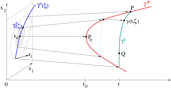
Figure 5: Here $\gamma^{*}$ is the curve in the $x_{1}$-$x_{2}$ plane, constructed in Fig. 4. The image of $\gamma^{*}$ under the map $x\mapsto\bigl{(}\tau(x),x+\tau(x){\bf w}(x)\bigr{)}$ is a curve $\gamma^{\sharp}$ in $t$-$x$ space. At each time $t>t_{0}=\tau(x_{0})$, the singular curve $\gamma^{t}$ (where a positive amount of mass is concentrated) is parameterized by $\zeta\mapsto y(t,\zeta)$, where $\tau(\zeta)\leq t$. Here $y(t,\zeta)$ is the position at time $t$ of the particle which was located at $\gamma^{*}(\zeta)$ at the initial time $t=0$. The endpoints of $\gamma^{t}$ lie on $\gamma^{\sharp}$.

Similarly to the 1-dimensional case, for $t>t_{0}$ the singular curve $\gamma^{t}$ will be located within the region $V$ in the interior of the cusp covered by three sheets of characteristics. Based on this fact, we define the set

$$R~{}\doteq~{}\bigl{\{}(t,\xi,\sigma)\,;~{}\tau(\xi,\sigma)<t\bigr{\}},$$ (4.6)

and its boundary

$$\Sigma~{}\doteq~{}\bigl{\{}(t,\xi,\sigma)\,;~{}\tau(\xi,\sigma)=t\bigr{\}}.$$

For each $(t,\xi,\sigma)\in R$, there exist two other characteristics reaching the same point at time $t$. We call

$$\Big{(}\xi_{i}(t,\xi,\sigma)\,,~{}\sigma_{i}(t,\xi,\sigma)\Big{)},\qquad i=1,2,$$

the coordinates of the initial points of these characteristics. In other words, the points

$$x\bigl{(}\xi_{1}(t,\xi,\sigma),\,\sigma_{1}(t,\xi,\sigma)\bigr{)},\qquad x\bigl{(}\xi_{2}(t,\xi,\sigma),\,\sigma_{2}(t,\xi,\sigma)\bigr{)},$$ (4.7)

are the initial points of the additional two characteristics that at time $t$ reach the same point

$$y~{}=~{}x(\xi,\sigma)+t\,{\bf w}\bigl{(}x(\xi,\sigma)\bigr{)}.$$ (4.8)

As a consequence, using the shorter notation introduced at (4.4), at time $t$ the values of the velocity ${\bf v}^{\pm}$ at the point $y$ are given by

$$\begin{array}[]{rl}{\bf v}^{-}(t,y)&=~{}{\bf w}\Big{(}\xi_{1}(t,\xi,\sigma),\,\sigma_{1}(t,\xi,\sigma)\Big{)},\\[8.53581pt] {\bf v}^{+}(t,y)&=~{}{\bf w}\Big{(}\xi_{2}(t,\xi,\sigma),\,\sigma_{2}(t,\xi,\sigma)\Big{)}.\end{array}$$ (4.9)

By (1.4), similar formulas can be obtained for the densities $\rho^{\pm}(t,y)$. Namely,

$$\begin{array}[]{rl}\rho^{-}(t,y)&\displaystyle=~{}\frac{\bar{\rho}\bigl{(}\xi_{1}(t,\xi,\sigma),\sigma_{1}(t,\xi,\sigma)\bigr{)}}{\det\Big{[}I+t\,D_{x}{\bf w}\bigl{(}\xi_{1}(t,\xi,\sigma),\sigma_{1}(t,\xi,\sigma)\bigr{)}\Big{]}},\\[11.38109pt] \rho^{+}(t,y)&\displaystyle=~{}\frac{\bar{\rho}\bigl{(}\xi_{2}(t,\xi,\sigma),\sigma_{2}(t,\xi,\sigma)\bigr{)}}{\det\Big{[}I+t\,D_{x}{\bf w}\bigl{(}\xi_{2}(t,\xi,\sigma),\sigma_{2}(t,\xi,\sigma)\bigr{)}\Big{]}}.\end{array}$$ (4.10)

We observe that, for $i=1,2$, the determinant is computed by

$$\begin{array}[]{l}\det\Big{[}I+t\,D_{x}{\bf w}\bigl{(}\xi_{i}(t,\xi,\sigma),\sigma_{i}(t,\xi,\sigma)\bigr{)}\Big{]}\\[8.53581pt] \qquad=~{}\Big{[}1+t\lambda_{1}\bigl{(}\xi_{i}(t,\xi,\sigma),\sigma_{i}(t,\xi,\sigma)\bigr{)}\Big{]}\Big{[}1+t\lambda_{2}\bigl{(}\xi_{i}(t,\xi,\sigma),\sigma_{i}(t,\xi,\sigma)\bigr{)}\Big{]}.\end{array}$$ (4.11)

The first factor on the right hand side approaches zero as $t\to{-1/\lambda_{1}}$, while the second one remains uniformly positive.

4.1 Constructing the points $x_{i}(t,\xi,\sigma)$.

Given $(t,\xi,\sigma)$, with $t>\tau(\xi,\sigma)$, we seek a formula describing the two points in (4.7). For $i=1,2$, the vector equation

$$x(\xi_{i},\sigma_{i})+t\,{\bf w}\bigl{(}x(\xi_{i},\sigma_{i})\bigr{)}~{}=~{}x(\xi,\sigma)+t\,{\bf w}\bigl{(}x(\xi,\sigma)\bigr{)}$$

is equivalent to two scalar equations, obtained by taking the inner products with $r_{1}(\xi)$ and with its orthogonal vector. Here and in the sequel, $r_{1}^{\perp}(\xi)$ denotes the unit vector obtained by rotating $r_{1}(\xi)$ counterclockwise by an angle $\pi/2$.

$$\left\{\begin{array}[]{rl}\Phi_{1}(t,\xi,\sigma,\xi_{i},\sigma_{i})&\doteq~{}\Big{\langle}r_{1}(\xi)\,,~{}x(\xi_{i},\sigma_{i})+t\,{\bf w}\bigl{(}x(\xi_{i},\sigma_{i})\bigr{)}-x(\xi,\sigma)-t\,{\bf w}\bigl{(}x(\xi,\sigma)\bigr{)}\Big{\rangle}~{}=~{}0,\\[11.38109pt] \Phi_{2}(t,\xi,\sigma,\xi_{i},\sigma_{i})&\doteq~{}\Big{\langle}r_{1}^{\perp}(\xi)\,,~{}x(\xi_{i},\sigma_{i})+t\,{\bf w}\bigl{(}x(\xi_{i},\sigma_{i})\bigr{)}-x(\xi,\sigma)-t\,{\bf w}\bigl{(}x(\xi,\sigma)\bigr{)}\Big{\rangle}~{}=~{}0.\end{array}\right.$$ (4.12)

The equations (4.12) have to be solved for the two variables $\xi_{i},\sigma_{i}$. Trivially,

$$\Phi_{1}(t,\xi,\sigma,\xi,\sigma)~{}=~{}\Phi_{2}(t,\xi,\sigma,\xi,\sigma)~{}=~{}0.$$

Of course, we are interested in the two additional nontrivial solutions. When $t=\tau(\xi)$, $\xi_{i}=\xi$ and $\sigma_{i}=\sigma=0$, we observe that the vector $r_{2}^{*}(\xi)={\partial\over\partial\xi}\gamma^{*}(\xi)$ introduced at (4.5) is not parallel to $r_{1}(\xi)$. Say,

$$r_{2}^{*}(\xi)~{}=~{}c_{1}(\xi)r_{1}(\xi)+c_{2}(\xi)r_{2}(\xi),$$ (4.13)

with $c_{2}(\xi)\not=0$. Therefore,

$$\begin{array}[]{rl}p_{0}(\xi)&\displaystyle\doteq~{}\frac{\partial\Phi_{2}}{\partial\xi_{i}}\bigl{(}\tau(\xi),\xi,0,\xi_{i},0\bigr{)}\bigg{|}_{\xi_{i}=\xi}\,=\,\Big{\langle}r_{1}^{\perp}(\xi),\,\bigl{(}I+\tau(\xi)D{\bf w}\bigr{)}r_{2}^{*}(\xi)\Big{\rangle}\\[8.53581pt] &=\,\Big{\langle}r_{1}^{\perp}(\xi),\,\bigl{(}1+\tau(\xi)\lambda_{2}(\xi)\bigr{)}c_{2}(\xi)r_{2}(\xi)\Big{\rangle}\,\neq\,0.\end{array}$$ (4.14)

The second equation in (4.12) can thus be solved for the variable $\xi_{i}$ by the implicit function theorem, say

$$\xi_{i}~{}=~{}\phi(t,\xi,\sigma,\sigma_{i}),$$ (4.15)

for some analytic function $\phi$ with

$$\phi\bigl{(}t,\xi,\sigma,\sigma\bigr{)}~{}=~{}\xi$$ (4.16)

for every $t,\xi,\sigma$. The following computations will yield a leading order expansion for the function $\phi$.

Since the map $\sigma\mapsto\tau(\xi,\sigma)=-1/\lambda_{1}(\xi,\sigma)$ has a positive local minimum at $\sigma=0$, a Taylor expansion yields

$$\lambda_{1}(\xi,\sigma)~{}=~{}-\omega_{1}(\xi)+\sum_{k\geq 3}\omega_{k}(\xi){\sigma^{k-1}\over(k-1)!}$$ (4.17)

for some analytic functions $\omega_{j}(\xi)$, with

$$\omega_{1}(\xi)\,>\,0,\qquad\qquad\omega_{3}(\xi)\,>\,0.$$

Note the close analogy with the one dimensional case considered at (3.4). In turn, (4.17) yields

$$\tau(\xi,\sigma)~{}=~{}-{1\over\lambda_{1}(\xi,\sigma)}~{}=~{}{1\over\omega_{1}(\xi)}\left(1+{\omega_{3}(\xi)\over\omega_{1}(\xi)}\sigma^{2}+{\cal O}(1)\cdot\sigma^{3}\right).$$ (4.18)

In addition, since all vectors $r_{1}(\xi,\sigma)$ have unit length and by definition $r_{1}(\xi,0)=r_{1}(\xi)$, we have

$$\begin{array}[]{l}\Big{\langle}r_{1}(\xi)~{},~{}r_{1}(\xi,\sigma)-r_{1}(\xi)\Big{\rangle}~{}=~{}q_{1}(\xi)\sigma^{2}+q_{2}(\xi)\sigma^{3}+{\cal O}(1)\sigma^{4},\\[11.38109pt] \Big{\langle}r_{1}^{\perp}(\xi)~{},~{}r_{1}(\xi,\sigma)-r_{1}(\xi)\Big{\rangle}~{}=~{}q_{3}(\xi)\,\sigma+q_{4}(\xi)\,\sigma^{2}+{\cal O}(1)\cdot\sigma^{3},\end{array}$$ (4.19)

where

$$q_{1}(\xi)=\Big{\langle}r_{1}(\xi)~{},~{}\frac{1}{2}\frac{\partial^{2}r_{1}}{\partial\sigma^{2}}(\xi,0)\Big{\rangle},\qquad q_{3}(\xi)~{}\doteq~{}\Big{\langle}r_{1}^{\perp}(\xi)~{},~{}{\partial r_{1}\over\partial\sigma}(\xi,0)\Big{\rangle},$$ (4.20)

and similar formulas hold for $q_{2},q_{4}$. We now compute

$$\begin{array}[]{l}\displaystyle x(\xi,Z)+t{\bf w}\bigl{(}x(\xi,Z)\bigr{)}-x(\xi,\sigma)-t{\bf w}\bigl{(}x(\xi,\sigma)\bigr{)}~{}=~{}\int_{\sigma}^{Z}{d\over ds}\Big{[}x(\xi,s)+t\,{\bf w}\bigl{(}x(\xi,s)\bigr{)}\Big{]}\,ds\\[11.38109pt] \displaystyle=~{}\int_{\sigma}^{Z}\bigl{(}1+t\lambda_{1}(\xi,s)\bigr{)}r_{1}(\xi,s)\,ds\\[11.38109pt] \displaystyle=~{}\int_{\sigma}^{Z}\bigl{(}t-\tau(\xi)\bigr{)}\lambda_{1}(\xi,s)r_{1}(\xi,s)\,ds+\int_{\sigma}^{Z}\tau(\xi)\Big{[}\lambda_{1}(\xi,s)-\lambda_{1}(\xi)\Big{]}r_{1}(\xi,s)\,ds\,.\end{array}$$ (4.21)

Taking the inner product with $r_{1}^{\perp}(\xi)$, using (4.19) and observing that

$$\lambda_{1}(\xi,s)-\lambda_{1}(\xi)~{}=~{}\frac{\omega_{3}(\xi)}{2}s^{2}+\frac{\omega_{4}(\xi)}{6}s^{3}+\frac{\omega_{5}(\xi)}{24}s^{4}+{\cal O}(1)\cdot s^{5},$$

one obtains

$$\begin{array}[]{rl}\Phi_{2}\bigl{(}t,\xi,\sigma,\xi,Z\bigr{)}&=\displaystyle~{}\bigl{(}t-\tau(\xi)\bigr{)}\lambda_{1}(\xi)\Big{[}q_{3}(\xi){Z^{2}-\sigma^{2}\over 2}+q_{4}(\xi)\frac{Z^{3}-\sigma^{3}}{3}\Big{]}+\frac{\omega_{3}(\xi)}{8}\tau(\xi)q_{3}(\xi)\bigl{(}Z^{4}-\sigma^{4}\bigr{)}\\[8.53581pt] &\qquad\displaystyle+{\cal O}(1)\cdot\bigl{(}t-\tau(\xi)\bigr{)}\bigl{(}Z^{4}-\sigma^{4}\bigr{)}+\,{\cal O}(1)\cdot\bigl{(}Z^{5}-\sigma^{5}\bigr{)}.\end{array}$$ (4.22)

Recalling (4.20) and (4.14), we set

$$q_{5}(\xi)\doteq-{\lambda_{1}(\xi)\,q_{3}(\xi)\over 2p_{0}(\xi)},\qquad q_{6}(\xi)\doteq-\frac{\lambda_{1}(\xi)q_{4}(\xi)}{3p_{0}(\xi)},\qquad q_{7}(\xi)\doteq-\frac{\omega_{3}(\xi)\tau(\xi)q_{3}(\xi)}{8p_{0}(\xi)}.$$ (4.23)

In view of (4.22) and (4.14), by the implicit function theorem we conclude

$$\begin{array}[]{rl}\phi\bigl{(}t,\xi,\sigma,Z\bigr{)}-\xi&\displaystyle=~{}\bigl{(}t-\tau(\xi)\bigr{)}\Big{[}q_{5}(\xi)(Z^{2}-\sigma^{2})+q_{6}(\xi)(Z^{3}-\sigma^{3})\Big{]}+q_{7}(\xi)\bigl{(}Z^{4}-\sigma^{4}\bigr{)}\\[11.38109pt] &\qquad\displaystyle+{\cal O}(1)\cdot\bigl{(}t-\tau(\xi)\bigr{)}\bigl{(}Z^{4}-\sigma^{4}\bigr{)}+\,{\cal O}(1)\cdot\bigl{(}Z^{5}-\sigma^{5}\bigr{)}\\[8.53581pt] &\doteq~{}\phi_{0}\bigl{(}t,\xi,\sigma,Z\bigr{)}~{}=~{}{\cal O}(1)\cdot\bigl{(}t-\tau(\xi)\bigr{)}^{2}\,.\end{array}$$ (4.24)

Note that, in the case where the integral curves of $r_{1}$ are straight lines, that is: $r_{1}(\xi,\sigma)=r_{1}(\xi)$ for all $\sigma$, we trivially have $\phi_{0}(t,\xi,\sigma,Z)\equiv 0$. In particular, $q_{1}(\xi)=\cdots=q_{7}(\xi)=0$.

Next, inserting the value

$$\xi_{i}~{}=~{}\phi(t,\xi,\sigma,Z)~{}=~{}\xi+\phi_{0}(t,\xi,\sigma,Z)$$

in the first equation of (4.12), we recover a scalar equation for the single variable $Z\doteq\sigma_{i}$. This has the form

$$\begin{array}[]{l}\widetilde{\Phi}(t,\xi,\sigma,Z)~{}\doteq~{}\Phi_{1}\bigl{(}t,\xi,\sigma,\phi(t,\xi,\sigma,Z),Z\bigr{)}\\[11.38109pt] \quad=~{}\displaystyle\Big{\langle}r_{1}(\xi)\,,~{}x\bigl{(}\phi(t,\xi,\sigma,Z),Z\bigr{)}+t\,{\bf w}\bigl{(}x\bigl{(}\phi(t,\xi,\sigma,Z),Z\bigr{)}\bigr{)}-x(\xi,\sigma)-t\,{\bf w}\bigl{(}x(\xi,\sigma)\bigr{)}\Big{\rangle}~{}=~{}0.\end{array}$$ (4.25)

Notice that this is a scalar equation of cubic type, similar to (3.13). Indeed, when $\phi_{0}=0$, it reduces precisely to (3.13). Hence the solution would be given by the same formula as (3.32).

Using the approximation (4.17) together with (4.19), we obtain

$$\begin{array}[]{l}\displaystyle\widetilde{\Phi}(t,\xi,\sigma,\xi,Z)~{}\displaystyle=~{}\Big{\langle}r_{1}(\xi)\,,~{}x(\xi,Z)+t\,{\bf w}\bigl{(}x(\xi,Z)\bigr{)}-x(\xi,\sigma)-t\,{\bf w}\bigl{(}x(\xi,\sigma)\bigr{)}\Big{\rangle}\\[11.38109pt] \qquad+\Big{\langle}r_{1}(\xi)\,,~{}x\bigl{(}\phi(t,\xi,\sigma,Z),Z\bigr{)}+t\,{\bf w}\bigl{(}x\bigl{(}\phi(t,\xi,\sigma,Z),Z\bigr{)}\bigr{)}-x(\xi,Z)-t\,{\bf w}\bigl{(}x(\xi,Z)\bigr{)}\Big{\rangle}\\[11.38109pt] \quad=~{}A+B.\end{array}$$ (4.26)

Recalling that $\omega_{1}(\xi)=-\lambda_{1}(\xi)=1/\tau(\xi)$, we compute

$$\begin{array}[]{rl}A&=~{}\displaystyle\left\langle r_{1}(\xi)~{},~{}\int_{\sigma}^{Z}\bigl{(}1+t\lambda_{1}(\xi,s)\bigr{)}\,r_{1}(\xi,s)\,ds\right\rangle\\[11.38109pt] &=\displaystyle\int_{\sigma}^{Z}\bigl{(}1+t\lambda_{1}(\xi,s)\bigr{)}\,ds\\[11.38109pt] &\displaystyle\qquad+\left\langle r_{1}(\xi)~{},~{}\int_{\sigma}^{Z}\bigl{(}1+t\lambda_{1}(\xi)\bigr{)}\bigl{(}r_{1}(\xi,s)-r_{1}(\xi)\bigr{)},ds\right\rangle+{\cal O}(1)\cdot(Z-\sigma)\bigl{(}|Z|^{4}+|\sigma|^{4}\bigr{)}\\[11.38109pt] &=~{}\displaystyle-\omega_{1}(\xi)\bigl{(}t-\tau(\xi)\bigr{)}(Z-\sigma)+{t\,\omega_{3}(\xi)\over 6}\,(Z^{3}-\sigma^{3})+\frac{t\,\omega_{4}(\xi)}{24}\bigl{(}Z^{4}-\sigma^{4}\bigr{)}\\[11.38109pt] &\qquad\displaystyle-\omega_{1}(\xi)\bigl{(}t-\tau(\xi)\bigr{)}\biggl{[}\frac{q_{1}(\xi)}{3}\,(Z^{3}-\sigma^{3})+\frac{q_{2}(\xi)}{4}(Z^{4}-\sigma^{4})\bigg{]}\\[11.38109pt] &\qquad+{\cal O}(1)\cdot\bigl{(}t-\tau(\xi)\bigr{)}\bigl{(}Z^{4}-\sigma^{4}\bigr{)}+\,{\cal O}(1)\cdot\bigl{(}Z^{5}-\sigma^{5}\bigr{)},\end{array}$$ (4.27)

where $q_{1}(\xi),q_{2}(\xi)$ are the coefficients in the Taylor expansion at (4.19). Moreover,

$$\begin{array}[]{rl}B&=~{}\Big{\langle}r_{1}(\xi)\,,~{}\bigl{(}1+\tau(\xi)D{\bf w}(\xi)\bigr{)}r_{2}^{*}(\xi)\Big{\rangle}\phi_{0}(t,\xi,\sigma,Z)\\[8.53581pt] &\qquad+{\cal O}(1)\cdot\bigl{(}t-\tau(\xi)\bigr{)}\phi_{0}+{\cal O}(1)\cdot\phi_{0}^{2}+{\cal O}(1)\cdot\phi_{0}Z.\end{array}$$ (4.28)

To remove the trivial solution $Z=\sigma$, we divide (4.25) by $Z-\sigma$. In view of (4.24) we obtain

$$\begin{array}[]{rl}\displaystyle 0&=~{}\displaystyle\Phi(t,\xi,\sigma,Z)~{}\doteq~{}{\Phi_{1}\bigl{(}t,\xi,\sigma,\phi(t,\xi,\sigma,Z),Z\bigr{)}\over Z-\sigma}\\[11.38109pt] &=~{}\displaystyle-\omega_{1}(\xi)\bigl{(}t-\tau(\xi)\bigr{)}+{t\,\omega_{3}(\xi)\over 6}\,(Z^{2}+Z\sigma+\sigma^{2})+\frac{t\,\omega_{4}(\xi)}{24}(Z+\sigma)(Z^{2}+\sigma^{2})\\[11.38109pt] &\qquad\displaystyle-\omega_{1}(\xi)\bigl{(}t-\tau(\xi)\bigr{)}\biggl{[}\frac{q_{1}(\xi)}{3}\,(Z^{2}+Z\sigma+\sigma^{2})+\frac{q_{2}(\xi)}{4}(Z+\sigma)(Z^{2}+\sigma^{2})\bigg{]}\\[11.38109pt] &\qquad+q_{8}(\xi)\Big{\{}\bigl{(}t-\tau(\xi)\bigr{)}\Big{[}q_{5}(\xi)(Z+\sigma)+q_{6}(\xi)(Z^{2}+\sigma Z+\sigma^{2})\Big{]}+q_{7}(\xi)(Z+\sigma)\bigl{(}Z^{2}+\sigma^{2}\bigr{)}\Bigr{\}}\\[11.38109pt] &\displaystyle\qquad\qquad+{\cal O}(1)\cdot\bigl{(}t-\tau(\xi)\bigr{)}\bigl{(}|Z|^{3}+|\sigma|^{3}\bigr{)}+\,{\cal O}(1)\cdot\bigl{(}|Z|^{4}+|\sigma|^{4}\bigr{)},\end{array}$$ (4.29)

where

$$q_{8}(\xi)~{}\doteq~{}\Big{\langle}r_{1}(\xi)\,,~{}\bigl{(}I+\tau(\xi)D_{x}{\bf w}(\xi)\bigr{)}r_{2}^{*}(\xi)\Big{\rangle}.$$

Dividing all terms by $t\omega_{3}(\xi)/6$ and recalling that $\tau(\xi)\omega_{1}(\xi)=1$, we are led to the equation

$$\begin{array}[]{l}\displaystyle 0~{}=~{}f(t,\xi,\sigma,Z)~{}\doteq~{}(Z^{2}+Z\sigma+\sigma^{2})\displaystyle-{6\omega_{1}(\xi)\bigl{(}t-\tau(\xi)\bigr{)}\over t\,\omega_{3}(\xi)}+\frac{\omega_{4}(\xi)}{4\omega_{3}(\xi)}(Z+\sigma)(Z^{2}+\sigma^{2})\\[11.38109pt] \qquad\displaystyle-{6\omega_{1}(\xi)\bigl{(}t-\tau(\xi)\bigr{)}\over t\,\omega_{3}(\xi)}\biggl{[}\frac{q_{1}(\xi)}{3}\,(Z^{2}+Z\sigma+\sigma^{2})+\frac{q_{2}(\xi)}{4}(Z+\sigma)(Z^{2}+\sigma^{2})\bigg{]}\\[11.38109pt] \qquad\displaystyle+{6q_{8}(\xi)\over t\,\omega_{3}(\xi)}\left\{\bigl{(}t-\tau(\xi)\bigr{)}\Big{[}q_{5}(\xi)(Z+\sigma)+q_{6}(\xi)(Z^{2}+\sigma Z+\sigma^{2})\Big{]}+q_{7}(\xi)(Z+\sigma)\bigl{(}Z^{2}+\sigma^{2}\bigr{)}\right\}\\[11.38109pt] \displaystyle\qquad+{\cal E}(t,\xi,\sigma,Z),\end{array}$$ (4.30)

where ${\cal E}$ is an analytic function that collects higher order terms:

$${\cal E}(t,\xi,\sigma,Z)~{}\doteq~{}{\cal O}(1)\cdot\bigl{(}t-\tau(\xi)\bigr{)}\bigl{(}|Z|^{3}+|\sigma|^{3}\bigr{)}+\,{\cal O}(1)\cdot\bigl{(}|Z|^{4}+|\sigma|^{4}\bigr{)}.$$ (4.31)

Note that, if the integral curves of the eigenvector $r_{1}$ are straight lines, i.e. $r_{1}(\xi,\sigma)=r_{1}(\xi)$, then $q_{1}(\xi)=\cdots=q_{8}(\xi)=0$ and above formula reduces to (3.28), with $t_{0}=\tau(\xi)$.

Since (4.30) will be solved on a domain of the form

$${\cal D}~{}=~{}\Big{\{}(t,\xi,\sigma)\,;~{}~{}0<t-\tau(\xi)<\varepsilon,~{}~{}|\sigma|\leq M\,\bigl{(}t-\tau(\xi)\bigr{)}\Big{\}},$$ (4.32)

it will be useful to make the change of variable

$$\widetilde{\sigma}~{}=~{}{\sigma\over t-\tau(\xi)}\,.$$ (4.33)

Still in view of (4.32), we expect $Z={\cal O}(1)\cdot\bigl{(}t-\tau(\xi)\bigr{)}^{1/2}$. Using the elementary expansion

$${1\over t}~{}=~{}{1\over\tau(\xi)+\bigl{(}t-\tau(\xi)\bigr{)}}~{}=~{}{1\over\tau(\xi)}\cdot\sum_{k=0}^{\infty}\left(t-\tau(\xi)\over\tau(\xi)\right)^{k},\qquad\qquad{1\over\tau(\xi)}~{}=~{}\omega_{1}(\xi),$$

and arranging terms according to their order of magnitude, we write (4.30) in the form

$$\begin{array}[]{rl}\displaystyle 0&\displaystyle=~{}\bigg{\{}\Big{[}Z^{2}-c_{1}(\xi)\bigl{(}t-\tau(\xi)\bigr{)}\Big{]}+\Big{[}c_{2}(\xi,\widetilde{\sigma})\bigl{(}t-\tau(\xi)\bigr{)}Z+c_{3}(\xi)Z^{3}\Big{]}\bigg{\}}\\[11.38109pt] &\qquad\qquad\displaystyle+\sum_{j+(k/2)\geq 2,\;j>0}c_{jk}(\xi,\widehat{\sigma})\bigl{(}t-\tau(\xi)\bigr{)}^{j}Z^{k}\\[11.38109pt] &\doteq~{}\Gamma(t,\xi,\sigma,Z)+{\cal E}(t,\xi,\sigma,Z).\end{array}$$ (4.34)

Here

$$c_{1}(\xi)~{}=~{}{6\omega_{1}^{2}(\xi)\over\omega_{3}(\xi)}\,,\qquad\qquad c_{2}(\xi,\widetilde{\sigma})\,=\,\widetilde{\sigma}+{6q_{5}(\xi)q_{8}(\xi)\omega_{1}(\xi)\over\omega_{3}(\xi)},$$ (4.35)

$$c_{3}(\xi)\,=\,\frac{\omega_{4}(\xi)}{4\omega_{3}(\xi)}+\frac{6q_{7}(\xi)q_{8}(\xi)\omega_{1}(\xi)}{\omega_{3}(\xi)}\,,$$ (4.36)

while $c_{jk}(\xi,\widetilde{\sigma})$ are analytic functions.

Lemma 4.1

Given $\xi_{0},\widetilde{\sigma}_{0}$, there exist analytic functions $\beta_{0},\beta_{1}$ defined in a neighborhood of $\bigl{(}\tau(\xi_{0}),\xi_{0},\widetilde{\sigma}_{0}\bigr{)}$ such that the two solutions to (4.34) have the form

$$Z^{\pm}(t,\xi,\widetilde{\sigma})~{}=~{}\bigl{(}t-\tau(\xi)\bigr{)}\cdot\beta_{0}(t,\xi,\widetilde{\sigma})\,\pm\,\sqrt{t-\tau(\xi)}\cdot\beta_{1}(t,\xi,\widetilde{\sigma}).$$ (4.37)

The above coefficients satisfy

$$\beta_{0}(t,\xi,\widetilde{\sigma})~{}=~{}-{c_{2}(\xi,\widetilde{\sigma})+c_{1}(\xi)c_{3}(\xi)\over 2}+{\cal O}(1)\cdot\bigl{(}t-\tau(\xi)\bigr{)},$$ (4.38)

$$\beta_{1}(t,\xi,\widetilde{\sigma})~{}=~{}\sqrt{c_{1}(\xi)}+{\cal O}(1)\cdot\bigl{(}t-\tau(\xi)\bigr{)}.$$ (4.39)

Remark 4.1

It is worth noting that the formulas (4.37)–(4.39) reduce to (3.32)-(3.33) in the case where the integral curves of the eigenvectors $r_{1}$ are straight lines, so that $q_{1}(\xi)=\cdots=q_{8}(\xi)=0$.

Proof of Lemma 4.1.

1. To construct a solution to (4.34), we start with the approximation

$$Z~{}\approx~{}\pm\sqrt{c_{1}(\xi)\bigl{(}t-\tau(\xi)\bigr{)}}.$$

To the next order, inserting the above value to compute $Z^{3}$, we obtain an approximate solution to $\Gamma(t,\xi,\sigma,Z)=0$, namely

$$\begin{array}[]{rl}Z_{0}^{\pm}(t,\xi,\widetilde{\sigma})&\displaystyle\doteq\,-{\bigl{(}t-\tau(\xi)\bigr{)}c_{2}(\xi,\widetilde{\sigma})\over 2}\\[11.38109pt] &\qquad\displaystyle\pm{1\over 2}\sqrt{\bigl{[}\bigl{(}t-\tau(\xi)\bigr{)}c_{2}(\xi,\widetilde{\sigma})\bigr{]}^{2}+4c_{1}(\xi)\bigl{(}t-\tau(\xi)\bigr{)}\mp 4c_{3}(\xi)\bigl{[}c_{1}(\xi)(t-\tau(\xi))\bigr{]}^{3/2}}.\end{array}$$ (4.40)

We observe that the argument of the square root is a small perturbation of its leading term $4c_{1}(\xi)\bigl{(}t-\tau(\xi)\bigr{)}$. Expanding this argument in Taylor series, and collecting even and odd powers of $\bigl{(}t-\tau(\xi)\bigr{)}^{1/2}$, one can write (4.40) in the form

$$Z_{0}^{\pm}(t,\xi,\widetilde{\sigma})~{}=~{}b(t,\xi,\widetilde{\sigma})\cdot\bigl{(}t-\tau(\xi)\bigr{)}\pm h(t,\xi,\widetilde{\sigma})\cdot\sqrt{t-\tau(\xi)},$$ (4.41)

for suitable functions $b,h$, analytic on a neighborhood of $\bigl{(}\tau(\xi_{0}),\xi_{0},\widetilde{\sigma}_{0}\bigl{)}$. A more detailed expansion yields

$$\begin{array}[]{rl}Z_{0}^{\pm}(t,\xi,\widetilde{\sigma})&\displaystyle=~{}-{\bigl{(}t-\tau(\xi)\bigr{)}c_{2}(\xi,\widetilde{\sigma})\over 2}\pm\sqrt{c_{1}(\xi)\bigl{(}t-\tau(\xi)\bigr{)}}\cdot\sqrt{1\mp c_{3}(\xi)\left[c_{1}(\xi)\bigl{(}t-\tau(\xi)\bigr{)}\right]^{1/2}}\\[11.38109pt] &\qquad+{\cal O}(1)\cdot\bigl{(}t-\tau(\xi)\bigr{)}^{3/2}\\[11.38109pt] &\displaystyle=\,-{\bigl{(}t-\tau(\xi)\bigr{)}c_{2}(\xi,\widetilde{\sigma})\over 2}\pm\sqrt{c_{1}(\xi)\bigl{(}t-\tau(\xi)\bigr{)}}-\frac{c_{1}(\xi)}{2}c_{3}(\xi)\bigl{(}t-\tau(\xi)\bigr{)}\\[11.38109pt] &\qquad+{\cal O}(1)\cdot\bigl{(}t-\tau(\xi)\bigr{)}^{3/2}.\end{array}$$ (4.42)

Therefore, in (4.41) one has

$$b(t,\xi,\widetilde{\sigma})~{}=~{}-{c_{2}(\xi,\widetilde{\sigma})+c_{1}(\xi)c_{3}(\xi)\over 2}+{\cal O}(1)\cdot\bigl{(}t-\tau(\xi)\bigr{)},$$ (4.43)

$$h(t,\xi,\widetilde{\sigma})~{}=~{}\sqrt{c_{1}(\xi)}+{\cal O}(1)\cdot\bigl{(}t-\tau(\xi)\bigr{)}.$$ (4.44)

Recalling (4.35)-(4.36), we see that the above formulas reduce to (3.32)-(3.33) if the integral curves of $r_{1}(x)$ are straight lines, so that $q_{1}(\xi)=\cdots=q_{8}(\xi)$.

2. Starting with $Z_{0}$ as a first approximation, and applying Newton’s iterative algorithm, we obtain a sequence of approximations inductively defined as

$$Z_{n+1}~{}=~{}Z_{n}-{(\Gamma+{\cal E})(t,\xi,\widetilde{\sigma},Z_{n})\over\partial_{Z}(\Gamma+{\cal E})(t,\xi,\widetilde{\sigma},Z_{n})}\,.$$ (4.45)

We claim that this sequence is uniformly convergent on a neighborhood of $\bigl{(}\tau(\xi_{0}),\xi_{0},\widetilde{\sigma}_{0}\bigl{)}$. Indeed

• By construction, the functions $Z_{0}^{\pm}$ satisfy an equation of the form

  $$\begin{array}[]{rl}(\Gamma+{\cal E})(t,\xi,\widetilde{\sigma},Z_{0}^{\pm})&\displaystyle=\sum_{j+(k/2)\geq 2,\,j>0}c_{jk}(\xi,\widetilde{\sigma})\bigl{(}t-\tau(\xi)\bigr{)}^{j}(Z_{0}^{\pm})^{k}~{}=~{}{\cal O}(1)\cdot\bigl{(}t-\tau(\xi)\bigr{)}^{2}.\end{array}$$ (4.46)

• At the point $(t,\xi,\widetilde{\sigma},Z_{0}^{\pm})$ the partial derivative $\partial_{Z}(\Gamma+{\cal E})$ is bounded away from zero. Indeed, differentiating (4.34) w.r.t. $Z$ one obtains

  $$\partial_{Z}(\Gamma+{\cal E})(t,\xi,\widetilde{\sigma},Z)~{}=~{}2Z+\sum_{j+(k/2)\geq 2}c_{jk}(\xi,\widetilde{\sigma})\bigl{(}t-\tau(\xi)\bigr{)}^{j}\cdot k\,Z^{k-1}.$$

  Therefore, for $(t,\xi,\widetilde{\sigma})$ in a neighborhood of $\bigl{(}\tau(\xi_{0}),\xi_{0},\widetilde{\sigma}_{0}\bigl{)}$, there exists a constant $\kappa_{0}>0$ such that

  $$\Big{|}\partial_{Z}(\Gamma+{\cal E})(t,\xi,\widetilde{\sigma},Z_{0}^{\pm})\Big{|}~{}\geq~{}\kappa_{0}\bigl{(}t-\tau(\xi)\bigr{)}^{1/2}.$$ (4.47)

• Finally, from (4.34) it is clear that the second derivative $\partial_{ZZ}(\Gamma+{\cal E})(t,\xi,\widetilde{\sigma},Z)$ is locally bounded

By Kantorovich’ theorem (see for example [4, 17]), the sequence $(Z_{n}^{\pm})_{n\geq 0}$ converges to a limit $Z^{\pm}=Z^{\pm}(t,\xi,\widetilde{\sigma})$ which provides a solution to (4.34). Moreover

$$\bigl{|}Z^{\pm}-Z_{0}^{\pm}\bigr{|}~{}=~{}{\cal O}(1)\cdot{(\Gamma+{\cal E})(t,\xi,\widetilde{\sigma},Z_{0}^{\pm})\over\partial_{Z}(\Gamma+{\cal E})(t,\xi,\widetilde{\sigma},Z_{0}^{\pm})}~{}\leq~{}\kappa_{1}\cdot\bigl{(}t-\tau(\xi)\bigr{)}^{3/2},$$ (4.48)

for some constant $\kappa_{1}$, uniformly valid on a neighborhood of $\bigl{(}\tau(\xi_{0}),\xi_{0},\widetilde{\sigma}_{0}\bigl{)}$. 3. It remains to check the regularity of the maps $Z^{\pm}(t,\xi,\widetilde{\sigma})$. Since the functions $\Gamma$, ${\cal E}$ are analytic, every iterate $Z_{n}^{\pm}$ can be written as a power series in $Z_{0}^{\pm}$,

$$Z_{n}^{\pm}~{}=~{}\sum_{j}c_{j}^{(n)}(t,\xi,\widetilde{\sigma})(Z_{0}^{\pm})^{j}.$$

By uniform convergence, the same holds for the limit:

$$Z^{\pm}~{}=~{}\sum_{j}c_{j}(t,\xi,\widetilde{\sigma})(Z_{0}^{\pm})^{j}.$$

Recalling (4.41), we can separate terms containing even or odd powers of $\sqrt{t-\tau(\xi)}$. This leads to (4.37). 4. Finally, the identities in (4.38-(4.39) follow from (4.43)-(4.44). MM     

In turn, (4.37) yields information about the velocity ${\bf v}^{\pm}$ and density function $\rho^{\pm}$, in a neighborhood of a point where the singularity is formed. As in (4.4), in the following we continue to use the shorter notation $\lambda_{1}(\xi)\doteq\lambda_{1}\bigl{(}\gamma_{1}^{*}(\xi)\bigr{)}$,   $\bar{\rho}(\xi)\doteq\bar{\rho}\bigl{(}\gamma_{1}^{*}(\xi)\bigr{)}$, etc$\ldots$

Lemma 4.2

Let $\xi_{0}$ and $\widetilde{\sigma}_{0}\in{\mathbb{R}}$ be given. Then there exist analytic functions ${\bf B}_{1},{\bf B}_{2},b_{1},b_{2}$, defined for $(t,\xi,\widetilde{\sigma})$ in a neighborhood of $\bigl{(}\tau(\xi_{0}),\xi_{0},\widetilde{\sigma}_{0}\bigr{)}$, such that the following holds.

For $t\geq\tau(\xi)$ and $\sigma=\bigl{(}t-\tau(\xi)\bigr{)}\widetilde{\sigma}$, one has

$${\bf v}^{\pm}(t,\xi,\sigma)-{\bf w}(\xi)~{}=~{}{\bf B}_{1}(t,\xi,\widetilde{\sigma})\cdot\bigl{(}t-\tau(\xi)\bigr{)}\pm{\bf B}_{2}(t,\xi,\widetilde{\sigma})\cdot\sqrt{t-\tau(\xi)}\,,$$ (4.49)

$$\rho^{\pm}(t,\xi,\sigma)~{}=~{}\frac{1}{t-\tau(\xi)}\Big{[}b_{1}(t,\xi,\widetilde{\sigma})\pm b_{2}(t,\xi,\widetilde{\sigma})\cdot\sqrt{t-\tau(\xi)}\Big{]}.$$ (4.50)

Moreover, recalling (4.35)-(4.36) one obtains

$${\bf B}_{2}(\tau(\xi),\xi,\widetilde{\sigma})\,=\,\sqrt{c_{1}(\xi)}\lambda_{1}(\xi)r_{1}(\xi)~{}=~{}-\omega_{1}^{2}(\xi)\sqrt{6\over\omega_{3}(\xi)}\,r_{1}(\xi)\,\not=\,0,$$ (4.51)

$$b_{1}(\tau(\xi),\xi,\widetilde{\sigma})~{}=~{}\frac{\bar{\rho}(\xi)}{2(\lambda_{2}(\xi)-\lambda_{1}(\xi))}\,>\,0.$$ (4.52)

Proof. 1. The representation (4.49) follows from

$${\bf v}^{\pm}(t,\xi,\sigma)~{}=~{}{\bf w}\bigl{(}X^{\pm}(t,\xi,\sigma)\bigr{)},$$ (4.53)

where

$$X^{\pm}(t,\xi,\sigma)~{}=~{}x\Big{(}\phi(t,\xi,\sigma,Z^{\pm}),\,Z^{\pm}\Big{)}$$ (4.54)

are the initial points of the two additional characteristics reaching the point $x(\xi,\sigma)+t{\bf w}\bigl{(}x(\xi,\sigma)\bigr{)}$ at time $t$.

In view of Lemma 4.1, the two functions $Z^{\pm}(t,\xi,\widetilde{\sigma})$ admit the analytic representation (4.37). Since the map $(\xi,\sigma)\mapsto x(\xi,\sigma)$ at (4.3) is analytic, and so is the map $\phi$ at (4.15), it is clear that the two composed maps in (4.53) can be represented as in (4.49).

Recalling (4.24) and (4.39), when $t=\tau(\xi)$ and hence $\sigma=\bigl{(}t-\tau(\xi)\bigr{)}\widetilde{\sigma}=0$, we obtain

$${\bf B}_{2}\bigl{(}\tau(\xi),\xi,\widetilde{\sigma}\bigr{)}~{}=~{}\beta_{1}\bigl{(}\tau(\xi),\xi,\widetilde{\sigma}\bigr{)}\,D{\bf w}(\xi)r_{1}(\xi)~{}=~{}\sqrt{c_{1}(\xi)}\lambda_{1}(\xi)r_{1}(\xi)~{}\not=~{}0.$$

In addition, since ${\bf B}_{1}$ collects even powers of $\sqrt{t-\tau(\xi)}$ and ${\bf B}_{1}\bigl{(}\tau(\xi),\xi,\widetilde{\sigma}\bigr{)}=0$, by analyticity the second estimate in (4.51) must hold.

Furthermore, by Taylor expansions we have the following leading order approximations:

$$\begin{array}[]{l}{\bf B}_{1}(t,\xi,\widetilde{\sigma})~{}\displaystyle=~{}\beta_{0}(t,\xi,\widetilde{\sigma})\lambda_{1}(\xi)r_{1}(\xi)\\[11.38109pt] \qquad\displaystyle+\frac{c_{1}(\xi)}{2}\Bigl{(}D^{2}{\bf w}(\xi)\bigl{(}r_{1}(\xi)\otimes r_{1}(\xi)\bigr{)}+D{\bf w}(\xi)\,\bigl{(}Dr_{1}(\xi)\cdot r_{1}(\xi)\bigr{)}\Bigr{)}+{\cal O}(1)\cdot\bigl{(}t-\tau(\xi)\bigr{)},\end{array}$$ (4.55)

$${\bf B}_{2}(t,\xi,\widetilde{\sigma})=\sqrt{c_{1}(\xi)}\lambda_{1}(\xi)r_{1}(\xi)+{\cal O}(1)\cdot\bigl{(}t-\tau(\xi)\bigr{)}.$$ (4.56)

2. To prove (4.50) we recall that, by (1.4) and (4.11),

$$\rho^{\pm}(t,\xi,\sigma)~{}=~{}{\bar{\rho}(X^{\pm})\over\det\bigl{(}I+tD{\bf w}(X^{\pm})\bigr{)}}~{}=~{}{\bar{\rho}(X^{\pm})\over 1+t\lambda_{2}\bigl{(}X^{\pm}\bigr{)}}\cdot{1\over 1+t\lambda_{1}\bigl{(}X^{\pm})}\,,$$ (4.57)

with $X^{\pm}$ as in (4.54). The same arguments as in step 1 yield the existence of scalar functions $\varphi_{1},\varphi_{2},\varphi_{3},\varphi_{4}$, analytic in a neighborhood of $\bigl{(}\tau(\xi_{0}),\xi_{0},\widetilde{\sigma}_{0}\bigr{)}$, such that

$${\bar{\rho}(X^{\pm})\over 1+t\lambda_{2}\bigl{(}X^{\pm}\bigr{)}}~{}=~{}\varphi_{1}(t,\xi,\widetilde{\sigma})\pm\sqrt{t-\tau(\xi)}\cdot\varphi_{2}(t,\xi,\widetilde{\sigma}),$$ (4.58)

$$1+t\lambda_{1}\bigl{(}X^{\pm})~{}=~{}\bigl{(}t-\tau(\xi)\bigr{)}\cdot\varphi_{3}(t,\xi,\widetilde{\sigma})\pm\sqrt{t-\tau(\xi)}\cdot\varphi_{4}(t,\xi,\widetilde{\sigma}).$$ (4.59)

To estimate the size of (4.59), and understand at what rate its inverse blows up, we compute

$$1+t\lambda_{1}\bigl{(}X^{\pm})~{}=~{}-\lambda_{1}(\xi)\tau(\xi)+t\lambda_{1}\bigl{(}X^{\pm})~{}=~{}\bigl{(}t-\tau(\xi)\bigr{)}\lambda_{1}(\xi)+t\Big{[}\lambda_{1}(X^{\pm})-\lambda_{1}(\xi)\Big{]}.$$ (4.60)

Recalling (4.17), (4.54), and the last estimate in (4.24), we obtain

$$\lambda_{1}(X^{\pm})-\lambda_{1}(\xi)~{}=~{}{\omega_{3}(\xi)\over 2}(Z^{\pm})^{2}+{\cal O}(1)\cdot\bigl{(}t-\tau(\xi)\bigr{)}^{3/2}.$$ (4.61)

Using Lemma 4.1 to compute $Z^{\pm}$, and recalling (4.35) and the identity $\tau(\xi)\omega_{1}(\xi)=1$, one obtains

$$\begin{array}[]{l}\displaystyle\bigl{(}t-\tau(\xi)\bigr{)}\lambda_{1}(\xi)+t\Big{[}\lambda_{1}(X^{\pm})-\lambda_{1}(\xi)\Big{]}\\[11.38109pt] \qquad\displaystyle=~{}-\omega_{1}(\xi)\bigl{(}t-\tau(\xi)\bigr{)}+\tau(\xi)\cdot{\omega_{3}(\xi)\over 2}\,c_{1}(\xi)\bigl{(}t-\tau(\xi)\bigr{)}+{\cal O}(1)\cdot(t-\tau(\xi))^{3/2}\\[11.38109pt] \qquad\displaystyle=~{}\left[-\omega_{1}(\xi)+{1\over\omega_{1}(\xi)}\cdot{\omega_{3}\over 2}\cdot{6\omega_{1}^{2}(\xi)\over\omega_{3}(\xi)}\right]\bigl{(}t-\tau(\xi)\bigr{)}+{\cal O}(1)\cdot\bigl{(}t-\tau(\xi)\bigr{)}^{3/2}\\[11.38109pt] =~{}\displaystyle 2\omega_{1}(\xi)\bigl{(}t-\tau(\xi)\bigr{)}+{\cal O}(1)\cdot\bigl{(}t-\tau(\xi)\bigr{)}^{3/2}.\end{array}$$ (4.62)

Therefore, the inverse of the quantity in (4.60) can be written as

$${1\over 1+t\lambda_{1}\bigl{(}X^{\pm})}~{}=~{}{1\over 2\omega_{1}(\xi)\bigl{(}t-\tau(\xi)\bigr{)}}\cdot\left(1+\sum_{k\geq 1}d_{k}\bigl{(}t-\tau(\xi)\bigr{)}^{k/2}\right).$$ (4.63)

Together with (4.58), this yields (4.50). Since we assume that the initial density $\bar{\rho}$ is uniformly positive, taking the limit as $t\to\tau(\xi)+$, the previous analysis yields

$$b_{1}\bigl{(}\tau(\xi),\xi,\widetilde{\sigma}\bigr{)}~{}=~{}\frac{\tau(\xi)}{2}\cdot{\bar{\rho}(\xi)\over 1+\tau(\xi)\lambda_{2}(\xi)}~{}=~{}\frac{\bar{\rho}(\xi)}{2\bigl{(}\lambda_{2}(\xi)-\lambda_{1}(\xi)\bigr{)}}~{}>~{}0.$$ (4.64)

Indeed, $\tau(\xi)=-1/\lambda_{1}(\xi)$ and $\lambda_{2}(\xi)>\lambda_{1}(\xi)$. MM     

5 Local construction of the singular curve

In view of (2.4), (2.6), we seek a solution $(y,\eta,{\bf v})(t,\zeta)\in{\mathbb{R}}^{2}\times{\mathbb{R}}\times{\mathbb{R}}^{2}$ of the system

$$\left\{\begin{array}[]{rl}\eta_{t}&=~{}\rho^{+}({\bf v}-{\bf v}^{+})\times y_{\zeta}+\rho^{-}({\bf v}^{-}-{\bf v})\times y_{\zeta}\,,\\[5.69054pt] y_{t}&=~{}{\bf v},\\[5.69054pt] {\bf v}_{t}&=~{}\displaystyle\rho^{+}\Big{(}({\bf v}-{\bf v}^{+})\times y_{\zeta}\Big{)}\,{{\bf v}^{+}-{\bf v}\over\eta}+\rho^{-}\Big{(}({\bf v}^{-}-{\bf v})\times y_{\zeta}\Big{)}\,{{\bf v}^{-}-{\bf v}\over\eta}\,.\end{array}\right.$$ (5.1)

The boundary data are

$$\left\{\begin{array}[]{rl}y(\tau(\zeta),\zeta)&=~{}\gamma^{\sharp}(\zeta)~{}\doteq~{}\gamma^{*}(\zeta)+\tau(\zeta){\bf w}(\gamma^{*}(\zeta)),\\[5.69054pt] \eta(\tau(\zeta),\zeta)&=~{}0,\\[5.69054pt] {\bf v}(\tau(\zeta),\zeta)&=~{}{\bf w}(\gamma^{*}(\zeta)).\end{array}\right.$$ (5.2)

Here we use $t,\zeta$ as independent variables to describe points on the singular curve (see Fig. 5). For a fixed $\zeta$, the map $t\mapsto y(t,\zeta)$, with $t\geq\tau(\zeta)$, describes the trajectory of a point on the singular curve. More precisely, consider the particle that at time $t=0$ was located at $\gamma^{*}(\zeta)$.

• During the time interval $t\in\bigl{[}0,\tau(\zeta)\bigr{]}$, this particle moves with constant speed ${\bf w}\bigl{(}\gamma^{*}(\zeta)\bigr{)}$.

• At time $t=\tau(\zeta)$, this particle is located at $\gamma^{\sharp}(\zeta)$, which is one of the endpoints of the singular curve $\gamma^{t}$.

• At times $t>\tau(\zeta)$ this same particle is located at a point $y(t,\zeta)$ on the singular curve $\gamma^{t}$.

Notice that, at a fixed time $t>t_{0}$, the singular curve is parameterized by the map $\zeta\mapsto y(t,\zeta)$. Here $\zeta$ ranges over the set $\bigl{\{}\zeta\,;~{}\tau(\zeta)\leq t\bigr{\}}$.

To state the main result, providing an asymptotic description of the initial stages of the singular curve, we need to work in a suitable space of analytic vector fields. More precisely, we fix a closed ball ${\cal B}=\{x\in{\mathbb{R}}^{2}\,;~{}|x|\leq r_{0}\}$ and a constant $\varrho>0$. We call $X_{{\cal B},\varrho}$ the space of all analytic functions $\phi:{\mathbb{R}}^{2}\mapsto{\mathbb{R}}$ such that

$$\|\phi\|_{{\cal B},\varrho}~{}\doteq~{}\sum_{n=0}^{\infty}{\varrho^{n}\over n!}\max_{|\alpha|=n}\sup_{x\in{\cal B}}\bigl{|}D^{\alpha}\phi(x)\bigr{|}~{}<~{}+\infty.$$ (5.3)

Here $\alpha=(\alpha_{1},\alpha_{2})$ is a multi-index, while $D^{\alpha}\phi\doteq\partial_{x_{1}}^{\alpha_{1}}\partial_{x_{2}}^{\alpha_{2}}\phi$. Notice that this is the set of all functions whose Taylor series at every point $x\in{\cal B}$ converges on a disc of radius $\varrho/2$.

In the following theorem, we consider the space of all initial data $({\bf w},\bar{\rho})=(w_{1},w_{2},\bar{\rho})$ such that $w_{1},w_{2},\bar{\rho}\in X_{{\cal B},\varrho}$, for some given ${\cal B},\varrho$. Within this space, we will construct piecewise analytic solutions to the equations of pressureless gases (1.1)-(1.2) beyond singularity formation, for a generic set of initial data.

Theorem 5.1

For the Cauchy problem (1.1)-(1.2), assume that the initial data are analytic functions, satisfying (A1)-(A2).

Then an analytic solution up to some time $t_{0}$ where the ${\cal C}^{1}$ norm of the velocity ${\bf v}$ blows up. This solution can be extended to a larger interval $[0,t_{0}+\varepsilon_{0}]$. For $t_{0}<t\leq t_{0}+\varepsilon_{0}$ the solution is piecewise analytic, and contains a singular curve $\gamma^{t}$ where a positive amount of mass is concentrated.

Proof. The analysis of solutions up to the first time $t_{0}$ when a singularity appears, so that $\bigl{\|}{\bf v}(t,\cdot)\bigr{\|}_{{\cal C}^{1}}\to+\infty$ and $\bigl{\|}\rho(t,\cdot)\bigr{\|}_{{\bf L}^{\infty}}\to+\infty$, has been worked out in the recent paper [7]. The following proof will focus on the construction of a local solution for $t\geq t_{0}$. To help the reader, we summarize the main steps.

• By a suitable change of variables, the equations in (5.1)-(5.2) are written as a system of 5 first order equations (5.26)–(5.30), with initial data (5.31)-(5.32).

• In turn, this system can be put in the standard form (5.57). An integrability condition near $T=0$ allows us to uniquely determine the initial values $\rho_{0},S_{0},Z_{0}$ in (5.32).

• By checking that none of the eigenvalues of the $5\times 5$ matrix ${\bf\Lambda}(\zeta)=\frac{\partial{\bf H}}{\partial{\bf u}}(0,\zeta,0,0)$ in (5.61) is a positive integer, we show that the system (5.57) is of Briot-Bouquet type. The general result in [26] can thus be applied, yielding the local existence of an analytic solution.

1. As in (4.8), a point $(t,y)\in[0,T]\times{\mathbb{R}}^{2}$ will be described in terms of the variables $(t,\xi,\sigma)$. These are uniquely determined by the requirements

$$y~{}=~{}x(\xi,\sigma)+t{\bf w}\bigl{(}x(\xi,\sigma)\bigr{)},\qquad\qquad\tau\bigl{(}x(\xi,\sigma)\bigr{)}<t.$$ (5.4)

The main advantage of these variables is that now we can use the expressions (4.54) for the initial points of the additional two characteristics that meet at $(t,y)$. In turn, the formulas (4.49)-(4.50) in Lemma 4.2 yield an accurate asymptotic description of the functions ${\bf v}^{\pm},\rho^{\pm}$, near the singularity. Starting from the system (5.1), we seek a system of equations for the variables $(\xi,\sigma,\eta)$ as functions of $(t,\zeta)$, where $(t,x(\xi,\sigma))\in R$ is related to $(t,y)$ by (4.8). Differentiating (5.4), one obtains

$$\left\{\begin{array}[]{rl}y_{t}&=~{}{\bf w}+(I+tD_{x}{\bf w})\cdot(x_{\xi}\xi_{t}+x_{\sigma}\sigma_{t}),\\[8.53581pt] y_{\zeta}&=~{}(I+tD_{x}{\bf w})\cdot(x_{\xi}\xi_{\zeta}+x_{\sigma}\sigma_{\zeta}),\\[8.53581pt] y_{tt}&=~{}2D_{x}{\bf w}\cdot(x_{\xi}\xi_{t}+x_{\sigma}\sigma_{t})+(x_{\xi}\xi_{t}+x_{\sigma}\sigma_{t})^{T}(t\,D^{2}{\bf w})(x_{\xi}\xi_{t}+x_{\sigma}\sigma_{t})\\[11.38109pt] &\qquad+(I+tD_{x}{\bf w})\cdot\bigl{(}x_{\xi}\xi_{tt}+x_{\sigma}\sigma_{tt}+x_{\xi\xi}\xi_{t}^{2}+2x_{\xi\sigma}\xi_{t}\sigma_{t}+x_{\sigma\sigma}\sigma_{t}^{2}\bigr{)}.\end{array}\right.$$ (5.5)

The first equation in (5.1) yields

$$\begin{array}[]{rl}\eta_{t}&=~{}\bigg{\{}\rho^{+}({\bf w}-{\bf v}^{+})+\rho^{-}({\bf v}^{-}-{\bf w})+(I+tD_{x}{\bf w})\cdot(x_{\xi}\xi_{t}+x_{\sigma}\sigma_{t})(\rho^{+}-\rho^{-})\bigg{\}}\\[8.53581pt] &\qquad\qquad\times(I+tD_{x}{\bf w})\cdot(x_{\xi}\xi_{\zeta}+x_{\sigma}\sigma_{\zeta})\\[8.53581pt] &\doteq~{}H(t,\xi,\sigma,\xi_{t},\sigma_{t},\xi_{\zeta},\sigma_{\zeta}).\end{array}$$ (5.6)

Since ${\bf v}_{t}=y_{tt}$, by (5.5), the last equation in (5.1) yields

$$\begin{array}[]{l}(I+tD_{x}{\bf w})\cdot(x_{\xi}\xi_{tt}+x_{\sigma}\sigma_{tt})\\[11.38109pt] \qquad=~{}-2D_{x}{\bf w}\cdot(x_{\xi}\xi_{t}+x_{\sigma}\sigma_{t})-(t\,D^{2}{\bf w})\bigl{(}(x_{\xi}\xi_{t}+x_{\sigma}\sigma_{t})\otimes(x_{\xi}\xi_{t}+x_{\sigma}\sigma_{t})\bigr{)}\\[11.38109pt] \qquad\qquad-(I+tD_{x}{\bf w})\cdot(x_{\xi\xi}\xi_{t}^{2}+2x_{\xi\sigma}\xi_{t}\sigma_{t}+x_{\sigma\sigma}\sigma_{t}^{2})\\[11.38109pt] \qquad\qquad\displaystyle+{1\over\eta}\bigg{\{}\bigl{(}(y_{t}-{\bf v}^{+})\times y_{\zeta}\bigr{)}\rho^{+}({\bf v}^{+}-y_{t})+\bigl{(}({\bf v}^{-}-y_{t})\times y_{\zeta}\bigr{)}\rho^{-}({\bf v}^{-}-y_{t})\bigg{\}}\\[11.38109pt] \displaystyle\qquad\doteq~{}F(t,\xi,\sigma,\xi_{t},\sigma_{t})+{1\over\eta}G(t,\xi,\sigma,\xi_{t},\sigma_{t},\xi_{\zeta},\sigma_{\zeta}),\end{array}$$ (5.7)

where $y_{\zeta},y_{t}$ are also computed by the first two equations in (5.5).

2. In order to replace the vector equation (5.7) with a couple of scalar equations, we consider the vectors

$$r_{1}(\xi,\sigma)~{}\doteq~{}{\partial\over\partial\sigma}x(\xi,\sigma),\qquad\qquad r_{2}^{*}(\xi,\sigma)~{}\doteq~{}{\partial\over\partial\xi}x(\xi,\sigma).$$ (5.8)

By (4.3), $r_{1}(\sigma,\xi)$ is a unit eigenvector of the Jacobian matrix $D{\bf w}$ at the point $x(\xi,\sigma)$, corresponding to the first eigenvalue $\lambda_{1}$. However, $r_{2}^{*}$ is not an eigenvector, in general. We denote by $r_{2}$ the unit eigenvector of $D{\bf w}$ corresponding to the second eigenvalue $\lambda_{2}$. In addition, we denote by $\{l_{1},l_{2}\}$ the dual basis of $\{r_{1},r_{2}\}$, and by $\{l_{1}^{*},l_{2}^{*}\}$ the dual basis of $\{r_{1},r_{2}^{*}\}$ so that

$$\langle l_{1}^{*},x_{\sigma}\rangle\,=\,\langle l_{2}^{*},x_{\xi}\rangle\,=\,1,\qquad\qquad\langle l_{1}^{*},x_{\xi}\rangle\,=\,\langle l_{2}^{*},x_{\sigma}\rangle\,=\,0.$$

Notice that $l_{1},l_{2}$ are left eigenvectors of $D_{x}{\bf w}$ corresponding to the eigenvalues $\lambda_{1}<\lambda_{2}$, respectively. Moreover, $l_{2}^{*}$ is also a left eigenvector with eigenvalue $\lambda_{2}$. However, $l_{1}^{*}$ is not an eigenvector, in general. Multiplying both sides of (5.7) by the inverse matrix $(I+tD_{x}{\bf w})^{-1}$ and taking the inner products with $l_{1}^{*},l_{2}^{*}$, one obtains two scalar equations for $\xi_{tt}$ and $\sigma_{tt}$.

Combined with (5.6), these yield the system

$$\left\{\begin{array}[]{rl}\eta_{t}&=~{}H,\\[8.53581pt] \sigma_{tt}&=~{}l_{1}^{*}\cdot(I+tD_{x}{\bf w})^{-1}\bigl{[}F+\eta^{-1}G\bigr{]},\\[8.53581pt] \xi_{tt}&\displaystyle=~{}{1\over 1+t\lambda_{2}}\,l_{2}^{*}\cdot\bigl{[}F+\eta^{-1}G\bigr{]},\end{array}\right.$$ (5.9)

where $H,F,G$ are the functions introduced at (5.6)-(5.7). Note the the second equation in (5.9) can be equivalently written as

$$\sigma_{tt}~{}=~{}\frac{1}{1+t\lambda_{1}}\,l_{1}\cdot\bigl{[}F+\eta^{-1}G\bigr{]}+\frac{l_{1}^{*}\cdot r_{2}}{1+t\lambda_{2}}\,l_{2}\cdot\bigl{[}F+\eta^{-1}G\bigr{]}.$$ (5.10)

3. Our next goal is to write the system (5.9) in a more standard form, to which a general existence-uniqueness theorem can then be applied. Here the main difficulty lies in the singularities along the initial curve where $t=\tau(\zeta)$. Indeed, the functions $F,G,H$ are not analytic, because some terms become unbounded as $t\to\tau(\zeta)$. Moreover, as shown in Lemma 4.2, the right hand sides of (4.49)-(4.50) contain a square root as a factor. To motivate our future choices of rescaled variables, it is useful to keep in mind the order of magnitude of the various quantities:

$$\eta~{}=~{}{\cal O}(1)\cdot\sqrt{t-\tau(\zeta)},\quad\qquad y_{t}-{\bf v}^{\pm}~{}=~{}{\cal O}(1)\cdot\sqrt{t-\tau(\zeta)},\qquad\quad\rho^{\pm}~{}=~{}{{\cal O}(1)\over t-\tau(\zeta)}\,.$$

We will write the equations (5.9) in a form where all the singularities arise in connection with negative powers of $t-\tau(\zeta)$. Toward this goal, we consider the rescaled variables

$$\widehat{\eta}\,=\,{\eta\over\sqrt{t-\tau(\zeta)}}\,,\qquad\quad\widehat{\xi}\,=\,{\xi-\zeta\over t-\tau(\zeta)},\qquad\quad\widehat{\sigma}\,=\,{\sigma\over t-\tau(\zeta)}\,.$$ (5.11)

In addition, to reduce the second order equations in (5.9) to a first order system, we introduce the variables

$$S\,=\,\sigma_{t}\,,\qquad\qquad Z\,=\,\xi_{t}\,.$$ (5.12)

Remark 5.1

The results in Lemma 4.2 describe the singularities of the functions ${\bf v}^{\pm},\rho^{\pm}$ in terms of the variables $(t,\xi,\widetilde{\sigma})$. However, we ultimately seek a solution in the form $(\xi,\sigma,\eta)=(\xi,\sigma,\eta)(t,\zeta)$. Toward this goal, it is convenient to express all the singular terms appearing in the equations as functions of the independent variables $t,\zeta$ (instead of $t,\xi$).

Notice the difference between $\widehat{\sigma}$ and the variable $\widetilde{\sigma}$ introduced at (4.33). Namely,

$$\widetilde{\sigma}~{}=~{}\frac{t-\tau(\zeta)}{t-\tau\bigl{(}\xi(t,\zeta)\bigr{)}}\cdot\widehat{\sigma}\,.$$

When $t=\tau(\zeta)$, the boundary condition yields $\xi\bigl{(}\tau(\zeta),\zeta\bigr{)}=\zeta$. Here the right hand side is analytic w.r.t. the variables $(t,\zeta,\xi,\widehat{\sigma})$, and hence also w.r.t. $(t,\zeta,\widehat{\xi},\widehat{\sigma})$

4. We now analyze the structure of $H,F$ and $G$ in (5.9). To simplify the notation, it will be convenient to write

$$\widehat{\bf B}_{1}~{}\doteq~{}\bigl{(}t-\tau(\xi)\bigr{)}{\bf B}_{1}\,.$$ (5.13)

Recalling the notations and results in Lemma 4.2, we have

$$H = \frac{1}{\sqrt{t-\tau(\xi)}}\cdot\bigg{\{}-2{\bf B}_{2}b_{1}-2\widehat{\bf B}_{1}b_{2}+2b_{2}(I+tD_{x}{\bf w})\cdot(x_{\xi}\xi_{t}+x_{\sigma}\sigma_{t})\bigg{\}}\times\Big{[}(I+tD_{x}{\bf w})\cdot(x_{\xi}\xi_{\zeta}+x_{\sigma}\sigma_{\zeta})\Big{]}$$

$$\doteq \frac{1}{\sqrt{t-\tau(\zeta)}}H_{1}(t,\zeta,\widehat{\xi},\widehat{\sigma},\xi_{t},\sigma_{t},\xi_{\zeta},\sigma_{\zeta}),$$

where

$$H_{1}=\sqrt{\frac{t-\tau(\zeta)}{t-\tau(\xi)}}\bigg{\{}-2{\bf B}_{2}b_{1}-2\widehat{\bf B}_{1}b_{2}+2b_{2}(I+tD_{x}{\bf w})\cdot(x_{\xi}\xi_{t}+x_{\sigma}\sigma_{t})\bigg{\}}\times\Big{[}(I+tD_{x}{\bf w})\cdot(x_{\xi}\xi_{\zeta}+x_{\sigma}\sigma_{\zeta})\Big{]}.$$ (5.14)

Observing that

$$\widehat{\eta}_{t}~{}=~{}{\eta_{t}\over\sqrt{t-\tau(\zeta)}}-{\widehat{\eta}\over 2\bigl{(}t-\tau(\zeta)\bigr{)}},$$

we obtain

$$\widehat{\eta}_{t}\,=\,\frac{H_{2}}{t-\tau(\zeta)},\qquad\qquad H_{2}\,\doteq\,H_{1}-\frac{\widehat{\eta}}{2}.$$ (5.15)

Next, we observe that $F$ in (5.7) is an analytic function of the variables $(t,\zeta,\widehat{\xi},\widehat{\sigma},\xi_{t},\sigma_{t})$. In particular, for a solution of the form

$$\sigma(t)~{}=~{}S_{0}\bigl{(}t-\tau(\xi)\bigr{)}+{\cal O}(1)\cdot\bigl{(}t-\tau(\xi)\bigr{)}^{2},\qquad\qquad\xi(t)~{}=~{}\xi_{0}+{\cal O}(1)\cdot\bigl{(}t-\tau(\xi)\bigr{)}^{2},$$

we have

$$F~{}=~{}2\omega_{1}(\xi_{0})S_{0}r_{1}(\xi_{0})+{\cal O}(1)\cdot\bigl{(}t-\tau(\xi)\bigr{)}.$$

By the first two equations in (5.5) and by Lemma 4.2 it follows

$$\left\{\begin{array}[]{rl}y_{t}-{\bf w}&=~{}(I+tD_{x}{\bf w})(x_{\xi}\xi_{t}+x_{\sigma}\sigma_{t})~{}\doteq~{}{\bf A}\,,\\[8.53581pt] {\bf v}^{\pm}-{\bf w}&=~{}\bigl{(}t-\tau(\xi)\bigr{)}{\bf B}_{1}\pm\sqrt{t-\tau(\xi)}\,{\bf B}_{2},\\[8.53581pt] y_{\zeta}&=~{}(I+tD_{x}{\bf w})(x_{\xi}\xi_{\zeta}+x_{\sigma}\sigma_{\zeta}),\\[11.38109pt] \rho^{\pm}&=\displaystyle~{}{b_{1}\pm b_{2}\sqrt{t-\tau(\xi)}\over t-\tau(\xi)}\,.\end{array}\right.$$ (5.16)

To leading order, i.e., neglecting terms of order ${\cal O}(1)\cdot\bigl{(}t-\tau(\xi)\bigr{)}^{3/2}$, recalling (4.38) and (4.35) we find

$${\bf A}~{}\approx~{}\bigl{(}1+t\lambda_{1}(\xi)\bigr{)}r_{1}(\xi)S_{0}~{}=~{}-\bigl{(}t-\tau(\xi)\bigr{)}\omega_{1}(\xi)r_{1}(\xi)S_{0}\,,$$ (5.17)

$$\begin{array}[]{rl}{\bf v}^{\pm}-{\bf w}&\approx~{}\lambda_{1}(\xi)\bigl{[}Z^{\pm}-\sigma\bigr{]}r_{1}(\xi)\\[5.69054pt] &\approx~{}-\omega_{1}(\xi)\left[\bigl{(}t-\tau(\xi)\bigr{)}\cdot\beta_{0}(t,\xi,\widetilde{\sigma})\,\pm\,\sqrt{t-\tau(\xi)}\cdot\beta_{1}(t,\xi,\widetilde{\sigma})-S_{0}\bigl{(}t-\tau(\xi)\bigr{)}\right]\\[5.69054pt] &\displaystyle\approx~{}-\omega_{1}(\xi)\left[-{3\over 2}S_{0}\bigl{(}t-\tau(\xi)\bigr{)}\pm\omega_{1}\sqrt{6\bigl{(}t-\tau(\xi)\bigr{)}\over\omega_{3}}-\widetilde{\phi}(\xi)\cdot\bigl{(}t-\tau(\xi)\bigr{)}\right]r_{1}(\xi).\end{array}$$ (5.18)

Here $\widetilde{\phi}$ collects terms that do not depend on $\sigma$. Notice that here ${\bf w}={\bf w}\bigl{(}x(\xi(t),\sigma(t))\bigr{)}$ must be computed along a solution of (5.9). Similarly, the values $Z^{\pm}$ also refer to this solution. For this reason, they are given by (4.37), with $\widetilde{\sigma}=S_{0}$.

Combining (5.17)-(5.18), we thus reach the expression

$$\begin{array}[]{rl}{\bf v}^{\pm}-y_{t}&=~{}\displaystyle\omega_{1}(\xi)\left[{5\over 2}S_{0}\bigl{(}t-\tau(\xi)\bigr{)}\mp\omega_{1}(\xi)\sqrt{6(t-\tau(\xi))\over\omega_{3}(\xi)}+\widetilde{\phi}(\xi)\cdot\bigl{(}t-\tau(\xi)\bigr{)}\right]r_{1}(\xi)\\[11.38109pt] &\qquad+{\cal O}(1)\cdot\bigl{(}t-\tau(\xi)\bigr{)}^{3/2}.\end{array}$$ (5.19)

We note that

$$\widehat{\bf B}_{1}\,=\,{\cal O}(1)\cdot\bigl{(}t-\tau(\xi)\bigr{)},\qquad{\bf B}_{2}~{}=~{}{\cal O}(1),\qquad{\bf A}\times y_{\zeta}\,=\,{\cal O}(1)\cdot\bigl{(}t-\tau(\xi)\bigr{)},$$ (5.20)

It then follows that

$$l_{1}^{*}\cdot(I+tD_{x}{\bf w})^{-1}G~{}=~{}{\cal O}(1)\cdot\bigl{(}t-\tau(\xi)\bigr{)}^{-1/2}.$$

In addition we have

$$l_{1}^{*}\cdot(I+tD_{x}{\bf w})^{-1}F~{}=~{}{\cal O}(1)\cdot\bigl{(}t-\tau(\xi)\bigr{)}^{-1}.$$

Since $l_{1}^{*}\cdot(I+tD_{x}{{\bf w}})^{-1}={\cal O}(1)\cdot(t-\tau(\xi))^{-1}$, recalling (5.9) and (5.12), we have

$$\sigma_{tt}~{}=~{}S_{t}\,=\,\frac{F_{1}}{t-\tau(\zeta)},$$ (5.21)

where

$$F_{1}\,\doteq\,(t-\tau(\zeta))l_{1}^{*}\cdot(I+tD_{x}{{\bf w}})^{-1}F+\sqrt{\frac{t-\tau(\zeta)}{t-\tau(\xi)}}\cdot\frac{1}{\widehat{\eta}}\,l_{1}^{*}\cdot(I+tD_{x}{{\bf w}})^{-1}G_{0}\,.$$ (5.22)

$$G_{0}\,\doteq\,\sqrt{t-\tau(\xi)}\cdot G.$$ (5.23)

In a similar way, the third equation in (5.9) now becomes

$$Z_{t}~{}=~{}\left(l_{2}^{*}\cdot r_{2}\right)\frac{l_{2}\cdot F}{1+t\lambda_{2}}+\left(l_{2}^{*}\cdot r_{2}\right)\frac{l_{2}\cdot G}{1+t\lambda_{2}}\frac{1}{\widehat{\eta}\sqrt{t-\tau(\zeta)}}~{}\doteq~{}F_{2}+\frac{G_{2}}{t-\tau(\zeta)},$$ (5.24)

where

$$F_{2}~{}=~{}\left(l_{2}^{*}\cdot r_{2}\right)\frac{l_{2}\cdot F}{1+t\lambda_{2}},\qquad\qquad G_{2}~{}=~{}\sqrt{\frac{t-\tau(\zeta)}{t-\tau(\xi)}}\,\frac{l_{2}^{*}\cdot r_{2}}{1+t\lambda_{2}}\,\frac{1}{\widehat{\eta}}\,l_{2}\cdot G_{0}\,,$$ (5.25)

are analytic functions of their arguments.

5. Summarizing the above discussion, the second order system (5.9) can be rewritten as a first order system of five equations. Namely

$$\widehat{\eta}_{t}~{}=~{}\frac{H_{2}}{t-\tau(\zeta)},\qquad\qquad H_{2}\doteq H_{1}-\frac{\widehat{\eta}}{2},$$ (5.26)

for a suitable analytic function $H_{1}$, together with

$$\widehat{\sigma}_{t}~{}=~{}{1\over t-\tau(\zeta)}(S-\widehat{\sigma}),$$ (5.27)

$$\widehat{\xi}_{t}~{}=~{}{1\over t-\tau(\zeta)}(Z-\widehat{\xi}),$$ (5.28)

$$S_{t}~{}=~{}{1\over t-\tau(\zeta)}F_{1}\bigl{(}t,\zeta,\widehat{\xi},\widehat{\sigma},\widehat{\eta},\xi_{t},\sigma_{t},\xi_{\zeta},\sigma_{\zeta}\bigr{)},$$ (5.29)

$$Z_{t}~{}=~{}F_{2}\bigl{(}t,\zeta,\widehat{\xi},\widehat{\sigma},\widehat{\eta},\xi_{t},\sigma_{t},\xi_{\zeta},\sigma_{\zeta}\bigr{)}+{1\over t-\tau(\zeta)}G_{2}\bigl{(}t,\zeta,\widehat{\xi},\widehat{\sigma},\xi_{t},\sigma_{t},\xi_{\zeta},\sigma_{\zeta}\bigr{)},$$ (5.30)

for suitable analytic functions $F_{1},F_{2},G_{2}$. Boundary conditions are assigned for $t=\tau(\zeta)$. In addition to

$$\eta\bigl{(}\tau(\zeta),\zeta\bigr{)}~{}=~{}\sigma\bigl{(}\tau(\zeta),\zeta\bigr{)}~{}=~{}0,\qquad\qquad\xi\bigl{(}\tau(\zeta),\zeta\bigr{)}~{}=~{}\zeta,$$ (5.31)

we impose the identities

$$\left\{\begin{array}[]{rll}\widehat{\eta}\bigl{(}\tau(\zeta),\zeta\bigr{)}&=~{}\varrho_{0}(\zeta),\\[8.53581pt] \widehat{\sigma}\bigl{(}\tau(\zeta),\zeta\bigr{)}&=~{}S\bigl{(}\tau(\zeta),\zeta\bigr{)}&=~{}S_{0}(\zeta),\\[8.53581pt] \widehat{\xi}\bigl{(}\tau(\zeta),\zeta\bigr{)}&=~{}Z\bigl{(}\tau(\zeta),\zeta\bigr{)}&=~{}Z_{0}(\zeta),\end{array}\right.$$ (5.32)

where the three functions $\varrho_{0},S_{0},Z_{0}$ are uniquely determined by the requirement that $H_{2},F_{1},G_{2}$ in (5.26), (5.29), (5.30) vanish at $t=\tau(\zeta)$. 6. In this step we show how to uniquely determine the initial data (5.32).

We begin by showing that $Z_{0}(\zeta)=0$. At $t=\tau(\zeta)$, by (5.25) the requirement $G_{2}=0$ is equivalent to $l_{2}\cdot G_{0}=0$. Recalling the bounds (5.20), from $l_{2}\cdot G_{0}=0$ we obtain

$$\big{(}{\bf B}_{2}\times y_{\zeta}\big{)}\big{(}l_{2}\cdot(\widehat{\bf B}_{1}-{\bf A})\big{)}=0.$$ (5.33)

We claim that ${\bf B}_{2}\times y_{\zeta}\neq 0$. Indeed, at $t=\tau(\zeta)$ one has $\xi_{\zeta}=1$, and hence by our assumptions it follows

$$\begin{array}[]{rl}{\bf B}_{2}\times y_{\zeta}&\displaystyle=~{}{\bf B}_{2}\times\Big{[}(I+\tau(\zeta)D_{x}{\bf w})\cdot r_{2}^{*}(\zeta)\Big{]}~{}=~{}\frac{1}{\lambda_{1}(\zeta)}{\bf B}_{2}\times\Big{[}\bigl{(}\lambda_{1}(\zeta)I-D_{x}{\bf w}\bigr{)}\cdot r_{2}^{*}(\zeta)\Big{]}\\[8.53581pt] &=\displaystyle~{}\sqrt{c_{1}(\zeta)}\,r_{1}(\zeta)\times\Big{[}\bigl{(}\lambda_{1}(\zeta)I-D_{x}{\bf w}\bigr{)}\cdot r_{2}^{*}(\zeta)\Big{]},\end{array}$$ (5.34)

which does not vanish, since $r_{2}^{*}$ is not parallel to $r_{1}$. Here $c_{1}(\cdot)$ is the function introduced at (4.35). Moreover, at $t=\tau(\zeta)$ we have

$$\begin{array}[]{rl}l_{2}\cdot(\widehat{\bf B}_{1}-{\bf A})&=\,\displaystyle-l_{2}\cdot(I+tD_{x}{\bf w})r_{2}^{*}(\zeta)Z_{0}(\zeta)\\[8.53581pt] &=\,\displaystyle-l_{2}\cdot\bigl{(}I-\frac{1}{\lambda_{1}(\zeta)}D_{x}{\bf w}\bigr{)}r_{2}^{*}(\zeta)Z_{0}(\zeta)\\[8.53581pt] &=\,\displaystyle-\frac{1}{\lambda_{1}(\zeta)}l_{2}\cdot\bigl{(}\lambda_{1}(\zeta)I-D_{x}{\bf w}\bigr{)}r_{2}^{*}(\zeta)Z_{0}(\zeta)\\[8.53581pt] &=\,\displaystyle-\frac{1}{\lambda_{1}(\zeta)}\bigl{(}\lambda_{1}(\zeta)-\lambda_{2}(\zeta)\bigr{)}l_{2}\cdot r_{2}^{*}(\zeta)Z_{0}(\zeta),\end{array}$$ (5.35)

because $l_{2}$ is a left eigenvector of $D_{x}{\bf w}$. Combining (5.33)–(5.35), we conclude that $Z_{0}(\zeta)=0$.

Next, we show how to determine $\varrho_{0}(\zeta)$. All computations are performed in the limit $t\to\tau(\zeta)$. Notice that in this case $\xi=\zeta$, hence $\tau(\xi)=\tau(\zeta)$.

The requirement $H_{2}=0$ implies $\varrho_{0}(\zeta)=2H_{1}.$ By (5.13) it trivially follows $\widehat{\bf B}_{1}={\cal O}(1)\cdot(t-\tau(\xi))$. Since $Z_{0}(\zeta)=0$, by (4.51) at $t=\tau(\zeta)$ we obtain

$$\begin{array}[]{rl}\varrho_{0}(\zeta)&=~{}2H_{1}~{}=\,-4b_{1}\,{\bf B}_{2}\times\Big{[}(I+\tau(\zeta)D_{x}{\bf w})r_{2}^{*}(\zeta)\Big{]}\\[11.38109pt] &~{}=\,-4b_{1}\sqrt{c_{1}(\zeta)}\,r_{1}(\zeta)\times\Big{[}(\lambda_{1}I-D_{x}{\bf w})r_{2}^{*}(\zeta)\Big{]}~{}>~{}0.\end{array}$$ (5.36)

Here the inequality $\varrho_{0}>0$ is intuitively obvious, because the density along the singular curve is initially zero and positive afterwards. A more detailed proof is achieved by observing that, at $t=\tau(\zeta)$, one has

$$r_{2}^{*}(\zeta)~{}=~{}a_{1}r_{1}(\zeta)+a_{2}r_{2}(\zeta),$$

with $a_{2}>0$. Recalling that $b_{1}$ is the positive constant at (4.64), the right hand side of (5.36) can be written as

$$-4b_{1}\sqrt{c_{1}(\zeta)}\,r_{1}(\zeta)\times\Big{[}(\lambda_{1}I-D_{x}{\bf w})a_{2}r_{2}(\zeta)\Big{]}~{}=\,-4b_{1}\sqrt{c_{1}(\zeta)}\,r_{1}(\zeta)\times\Big{[}(\lambda_{1}-\lambda_{2})a_{2}r_{2}(\zeta)\Big{]}~{}>~{}0.$$

Finally, in order to determine the initial value $S_{0}(\zeta)$, we need to use the assumption $F_{1}=0$ at $t=\tau(\zeta)$. Since $\widehat{\eta}=\varrho_{0}(\zeta)$ at $t=\tau(\zeta)$, one only needs to consider the equation

$$F_{1}~{}=~{}(t-\tau(\zeta))l_{1}^{*}\cdot(I+tD_{x}{{\bf w}})^{-1}F+\frac{1}{\varrho_{0}(\zeta)}\,l_{1}^{*}\cdot(I+tD_{x}{{\bf w}})^{-1}G_{0}~{}=~{}0\,.$$ (5.37)

Inserting the expression (5.7) for $F$ into the above equation and recalling that $Z_{0}(\zeta)=0$, always for $t=\tau(\zeta)$ we obtain

$$\begin{array}[]{l}\displaystyle(t-\tau(\zeta))l_{1}^{*}\cdot(I+tD_{x}{{\bf w}})^{-1}F\\[11.38109pt] \quad\displaystyle=(t-\tau(\zeta))l_{1}^{*}\cdot(I+tD_{x}{{\bf w}})^{-1}\Big{\{}-2D_{x}{\bf w}\cdot(x_{\xi}\xi_{t}+x_{\sigma}\sigma_{t})\\[11.38109pt] \qquad\qquad-(t\,D^{2}{\bf w})\bigl{(}(x_{\xi}\xi_{t}+x_{\sigma}\sigma_{t})\otimes(x_{\xi}\xi_{t}+x_{\sigma}\sigma_{t})\bigr{)}-(I+tD_{x}{\bf w})(x_{\xi\xi}\xi_{t}^{2}+2x_{\xi\sigma}\xi_{t}\sigma_{t}+x_{\sigma\sigma}\sigma_{t}^{2})\Big{\}}\\[11.38109pt] \quad\displaystyle=(t-\tau(\zeta))l_{1}^{*}\cdot(I+tD_{x}{{\bf w}})^{-1}\Big{\{}-2D_{x}{\bf w}\cdot r_{1}(\zeta)S_{0}(\zeta)-\tau(\zeta)S_{0}^{2}(\zeta)D^{2}{\bf w}(\zeta)\bigl{(}r_{1}(\zeta)\otimes r_{1}(\zeta)\bigr{)}\Big{\}}\\[11.38109pt] \quad\displaystyle=(t-\tau(\zeta))l_{1}^{*}\cdot(I+tD_{x}{{\bf w}})^{-1}\Big{\{}-2\lambda_{1}(\zeta)r_{1}(\zeta)S_{0}(\zeta)-\tau(\zeta)S_{0}^{2}(\zeta)D^{2}{\bf w}(\zeta)\bigl{(}r_{1}(\zeta)\otimes r_{1}(\zeta)\bigr{)}\Big{\}}\\[11.38109pt] \quad\displaystyle=~{}-2S_{0}(\zeta)-S_{0}^{2}(\zeta)\Big{[}\tau(\zeta)(t-\tau(\zeta))l_{1}^{*}\cdot(I+tD_{x}{{\bf w}})^{-1}r_{1}^{T}(\zeta)\,D^{2}{\bf w}\,r_{1}(\zeta)\Big{]},\end{array}$$ (5.38)

where we have used the identity

$$(t-\tau(\zeta))l_{1}^{*}\cdot(I+tD_{x}{{\bf w}})^{-1}r_{1}~{}=~{}\frac{1}{\lambda_{1}(\zeta)}.$$ (5.39)

At first sight, (5.38) looks like a quadratic equation for $S_{0}$. However, the following analysis reveals that as $t\to\tau(\zeta)$ the coefficient of $S_{0}^{2}$ vanishes, while the coefficient of $S_{0}$ is nonzero. Therefore, a unique value of $S_{0}(\zeta)$ is determined.

Indeed, consider the quantity

$$l_{1}^{*}\cdot(I+tD_{x}{\bf w})^{-1}(tD^{2}{\bf w})(r_{1}\otimes r_{1}).$$ (5.40)

For any vector ${\bf v}$, decomposing ${\bf v}$ along the basis of eigenvectors $\{r_{1},r_{2}\}$, one finds

$$(I+tD_{x}){\bf v}~{}=~{}(l_{1}\cdot{\bf v})(1+t\lambda_{1})r_{1}+(l_{2}\cdot{\bf v})(1+t\lambda_{2})r_{2}\,,$$

$$(I+tD_{x})^{-1}{\bf v}~{}=~{}(l_{1}\cdot{\bf v}){1\over 1+t\lambda_{1}}r_{1}+(l_{2}\cdot{\bf v}){1\over 1+t\lambda_{2}}r_{2}\,.$$

Therefore, the quantity in (5.40) can be rewritten as

$$l_{1}^{*}\cdot\left[{1\over 1+t\lambda_{1}}\Big{(}l_{1}\cdot(tD^{2}{\bf w})(r_{1}\otimes r_{1})\Big{)}r_{1}+{1\over 1+t\lambda_{2}}\Big{(}l_{2}\cdot(tD^{2}{\bf w})(r_{1}\otimes r_{1})\Big{)}r_{2}\right].$$ (5.41)

For $t\approx-1/\lambda_{1}$ the second term remains bounded, but the first term yields

$${1\over 1+t\lambda_{1}}\Big{(}l_{1}\cdot(tD^{2}{\bf w})(r_{1}\otimes r_{1})\Big{)}(l_{1}^{*}\cdot r_{1})~{}=~{}{1\over 1+t\lambda_{1}}\Big{(}l_{1}\cdot(tD^{2}{\bf w})(r_{1}\otimes r_{1})\Big{)}.$$

The following lemma allows us to compute the quantity $l_{1}\cdot(D^{2}{\bf w})(r_{1}\otimes r_{1})$.

Lemma 5.1

Let ${\bf w}(x)$ be a smooth vector field on ${\mathbb{R}}^{2}$. Assume that at each point $x\in{\mathbb{R}}^{2}$ its Jacobian matrix $D_{x}{\bf w}(x)$ has eigenvalues $\lambda_{1}(x)<\lambda_{2}(x)$, and a basis of right eigenvectors $\bigl{\{}r_{1}(x),r_{2}(x)\bigr{\}}$. Call $\bigl{\{}l_{1}(x),l_{2}(x)\bigr{\}}$ the dual basis of left eigenvectors.

Assume that at a point $\bar{x}$ we have $\nabla\lambda_{1}(\bar{x})\cdot r_{1}(\bar{x})=0$. Then

$$l_{1}(\bar{x})\cdot\Big{[}\bigl{(}D^{2}{\bf w}(\bar{x})\bigr{)}\bigl{(}r_{1}(\bar{x})\otimes r_{1}(\bar{x})\bigr{)}\Big{]}~{}=~{}0.$$ (5.42)

Proof. For any vector ${\bf v}\in{\mathbb{R}}^{2}$, the directional derivative of ${\bf w}$ in the direction of ${\bf v}$ at a point $x\in{\mathbb{R}}^{2}$ is computed by

$${d\over ds}{\bf w}(x+s{\bf v})\Bigg{|}_{s=0}~{}=~{}\lambda_{1}(x)\bigl{(}l_{1}(x)\cdot{\bf v}\bigr{)}r_{1}(x)+\lambda_{2}(x)\bigl{(}l_{2}(x)\cdot{\bf v}\bigr{)}r_{2}(x).$$

Calling $\bar{r}_{1}\doteq r_{1}(\bar{x})$, we need to compute the second derivative:

$$\begin{array}[]{l}\displaystyle\bigl{(}D^{2}{\bf w}(\bar{x})\bigr{)}\bigl{(}r_{1}(\bar{x})\otimes r_{1}(\bar{x})\bigr{)}~{}=~{}{d^{2}\over ds^{2}}{\bf w}(\bar{x}+s\bar{r}_{1})\Bigg{|}_{s=0}\\[11.38109pt] \displaystyle=~{}{d\over ds}\Big{[}\lambda_{1}(\bar{x}+s\bar{r}_{1})\bigl{(}l_{1}(\bar{x}+s\bar{r}_{1})\cdot\bar{r}_{1}\bigr{)}r_{1}(\bar{x}+s\bar{r}_{1})+\lambda_{2}(\bar{x}+s\bar{r}_{1})\bigl{(}l_{2}(\bar{x}+s\bar{r}_{1})\cdot\bar{r}_{1}\bigr{)}r_{2}(\bar{x}+s\bar{r}_{1})\Big{]}_{s=0}\end{array}$$ (5.43)

Since

$$l_{1}(\bar{x})\cdot r_{1}(\bar{x})\,=\,1,\qquad\qquad l_{1}(\bar{x})\cdot r_{2}(\bar{x})\,=\,0,\qquad\qquad\nabla\lambda(\bar{x})\cdot r_{1}(\bar{x})=0,$$

taking the product of the right hand side of (5.43) with $l_{1}(\bar{x})$ some terms clearly vanish. The remaining terms are computed by

$$\begin{array}[]{l}l_{1}(\bar{x})\cdot\Big{[}\bigl{(}D^{2}{\bf w}(\bar{x})\bigr{)}\bigl{(}r_{1}(\bar{x})\otimes r_{1}(\bar{x})\bigr{)}\Big{]}\\[8.53581pt] \displaystyle\quad=~{}\lambda_{1}(\bar{x})\left[{d\over ds}\bigl{(}l_{1}(\bar{x}+s\bar{r}_{1})\cdot\bar{r}_{1}\bigr{)}+l_{1}(\bar{x})\cdot{d\over ds}r_{1}(\bar{x}+s\bar{r}_{1})\right]_{s=0}\\[11.38109pt] \displaystyle\quad=~{}\lambda_{1}(\bar{x})\Big{[}{d\over ds}\bigl{(}l_{1}(\bar{x}+s\bar{r}_{1})\cdot r_{1}(\bar{x}+s\bar{r}_{1})\bigr{)}\Big{]}_{s=0}~{}=~{}0.\end{array}$$ (5.44)

MM     

By Lemma 5.1 together with (5.40)-(5.41) we conclude that, on the right hand side of (5.38), the term containing $S_{0}^{2}$ vanishes at $t=\tau(\zeta)$. Notice that this is entirely analogous to the 1-D case, where the terms containing $S^{2}$ on the right hand side of (3.47) vanish as $t\to t_{0}$.

By the previous analysis, the equation (5.37) further reduces to

$$-2S_{0}(\zeta)+\frac{1}{\varrho_{0}(\zeta)}\,l_{1}^{*}\cdot(I+tD_{x}{{\bf w}})^{-1}G_{0}~{}=~{}0\,.$$ (5.45)

We will show that (5.45) yields a linear equation for $S_{0}(\zeta)$, where the coefficient of $S_{0}$ does not vanish. This will uniquely determine $S_{0}$.

Toward this goal, note that $G_{0}=\sqrt{t-\tau(\xi)}\,G$, with

$$\begin{array}[]{rl}G&=~{}\bigl{(}({\bf v}^{-}-y_{t})\times y_{\zeta}\bigr{)}\rho^{-}({\bf v}^{-}-y_{t})-\bigl{(}({\bf v}^{+}-y_{t})\times y_{\zeta}\bigr{)}\rho^{+}({\bf v}^{+}-y_{t}).\end{array}$$ (5.46)

Therefore, in the expression of $G$ we should analyze the terms of order $\sqrt{t-\tau(\xi)}$ which also contain $S_{0}$, as $t\rightarrow\tau(\zeta)$. Based on (5.19) and Lemma 4.1, to leading order we compute

$$\begin{array}[]{rl}G&\displaystyle\approx~{}\omega_{1}^{2}\left[\frac{5}{2}S_{0}(t-\tau(\xi))+\omega_{1}\sqrt{\frac{6(t-\tau(\xi))}{\omega_{3}}}+\widetilde{\phi}(\xi)(t-\tau(\xi))\right]^{2}\cdot\bigl{(}r_{1}\times y_{\zeta}\bigr{)}\rho^{-}\,r_{1}\\[8.53581pt] &\displaystyle\qquad-\omega_{1}^{2}\left[\frac{5}{2}S_{0}(t-\tau(\xi))-\omega_{1}\sqrt{\frac{6(t-\tau(\xi))}{\omega_{3}}}+\widetilde{\phi}(\xi)(t-\tau(\xi))\right]^{2}\cdot\bigl{(}r_{1}\times y_{\zeta}\bigr{)}\rho^{+}\,r_{1}\\[8.53581pt] &\displaystyle=~{}\sqrt{t-\tau(\xi)}\omega_{1}^{2}\bigl{(}r_{1}\times y_{\zeta}\bigr{)}r_{1}\Bigl{\{}10b_{1}S_{0}\omega_{1}\sqrt{\frac{6}{\omega_{3}}}-b_{2}\frac{12\omega_{1}^{2}}{\omega_{3}}\Bigr{\}}+{\cal O}(1)(t-\tau(\xi))^{3/2}.\end{array}$$ (5.47)

Hence, using (5.47) and (5.39) we obtain

$$\begin{array}[]{rl}\displaystyle\frac{1}{\varrho_{0}(\zeta)}\,l_{1}^{*}\cdot(I+tD_{x}{{\bf w}})^{-1}G_{0}&\displaystyle=~{}\frac{\bigl{(}r_{1}\times y_{\zeta}\bigr{)}\omega_{1}^{2}}{-4b_{1}\sqrt{c_{1}(\zeta)}\;\lambda_{1}^{2}\bigl{(}r_{1}\times y_{\zeta}\bigr{)}}\left[10b_{1}S_{0}\omega_{1}\sqrt{\frac{6}{\omega_{3}}}-b_{2}\frac{12\omega_{1}^{2}}{\omega_{3}}\right]\\[11.38109pt] &=\displaystyle-\frac{10}{4}S_{0}+\frac{b_{2}}{2b_{1}}\sqrt{c_{1}},\end{array}$$ (5.48)

where we have made use of the formula for $\varrho_{0}(\zeta)$ at (5.36).

We claim that, at $t=\tau(\zeta)$,

$$\frac{b_{2}}{2b_{1}}\sqrt{c_{1}(\zeta)}~{}=~{}\frac{3}{4}S_{0}+\text{other terms independent of $S_{0}$}.$$ (5.49)

Indeed, since

$$\lambda_{1}(X^{\pm})-\lambda_{1}(\xi)=\frac{\omega_{3}}{2}\left(Z^{\pm}\right)^{2}+\frac{\omega_{4}}{6}\left(Z^{\pm}\right)^{3}+{\cal O}(1)\left(Z^{\pm}\right)^{4},$$

by Lemma 4.1 and (4.43)-(4.44) we have

$$\lambda_{1}(Z^{\pm})-\lambda_{1}(\xi)~{}=~{}\bigl{(}t-\tau(\xi)\bigr{)}\left\{\frac{\omega_{3}}{2}c_{1}(\xi)+{\cal O}(1)\bigl{(}t-\tau(\xi)\bigr{)}\right\}\pm\sqrt{t-\tau(\xi)}\Bigl{[}P+{\cal O}(1)\bigl{(}t-\tau(\xi)\bigr{)}\Bigr{]},$$

where

$$P~{}\doteq~{}\omega_{3}\sqrt{c_{1}(\xi)}\left(-{c_{2}(\xi,\widetilde{\sigma})+c_{1}(\xi)c_{3}(\xi)\over 2}\right)+\frac{\omega_{4}}{6}c_{1}(\xi)^{3/2}.$$

Therefore,

$$1+t\lambda_{1}(\xi,\sigma) = \frac{2}{\tau(\xi)}\bigl{(}t-\tau(\xi)\bigr{)}\left[1+{\cal O}(1)\bigl{(}t-\tau(\xi)\bigr{)}\pm\sqrt{t-\tau(\xi)}\Bigl{(}\frac{\tau(\xi)^{2}}{2}P+{\cal O}(1)\bigl{(}t-\tau(\xi)\bigr{)}\Bigr{)}\right]$$

$$\doteq \frac{2}{\tau(\xi)}\bigl{(}t-\tau(\xi)\bigr{)}\left[1+\phi_{3}\pm\sqrt{t-\tau(\xi)}\;\phi_{4}\right],$$

where $\phi_{3},\phi_{4}$ are analytic functions. It further implies

$$\frac{1}{1+t\lambda_{1}}=\frac{\tau(\xi)}{2\bigl{(}t-\tau(\xi)\bigr{)}}\Bigl{[}1\pm\sqrt{t-\tau(\xi)}\;\varphi_{0}\Bigr{]},$$ (5.50)

where $\varphi_{0}$ is an analytic function satisfying

$$t=\tau(\xi),\qquad\varphi_{0}=-\frac{\tau(\xi)^{2}}{2}\left(\omega_{3}\sqrt{c_{1}(\xi)}\,\Lambda+\frac{\omega_{4}}{6}c_{1}(\xi)^{3/2}\right).$$

Next, by (4.58) and (5.50) one obtains

$$b_{1}=\frac{\tau(\xi)}{2}\left[\varphi_{1}+(t-\tau(\xi))\varphi_{2}\varphi_{0}\right],\qquad b_{2}=\frac{\tau(\xi)}{2}\left[\varphi_{1}\varphi_{0}+\varphi_{2}\right].$$ (5.51)

Finally, at $t=\tau(\zeta)$ we obtain

$$\frac{b_{2}}{2b_{1}}\sqrt{c_{1}(\xi)} = \frac{(\varphi_{1}\varphi_{0}+\varphi_{2})\sqrt{c_{1}(\xi)}}{2[\varphi_{1}+(t-\tau(\xi))\varphi_{2}\varphi_{0}]}$$

$$= \sqrt{c_{1}(\zeta)}\left(\frac{\varphi_{0}}{2}+\frac{\varphi_{2}}{\varphi_{1}}\right)~{}=~{}-\frac{\tau(\zeta)^{2}}{4}c_{1}(\zeta)\omega_{3}\,\Lambda+\sqrt{c_{1}(\zeta)}\frac{\varphi_{2}}{\varphi_{1}}$$

$$= \frac{3}{4}S_{0}+\sqrt{c_{1}(\zeta)}\frac{\varphi_{2}}{\varphi_{1}},$$

as claimed in (5.49). We note that $\sqrt{c_{1}(\zeta)}\frac{\varphi_{2}}{\varphi_{1}}$ does not depend on $\widetilde{\sigma}$ at $t=\tau(\zeta)$.

Notice that the above result is consistent with what found in the 1-D case.

Thus, by combining (5.49) and (5.48) we conclude that the coefficient of $S_{0}$ in (5.45) is exactly $\frac{15}{4}$ as in 1-D case. Therefore, from the equation $F_{1}=0$ at $t=\tau(\zeta)$ a unique value of $S_{0}(\zeta)$ is determined.

7. We now perform a further renaming of variables, using

$$T\,=\,t-\tau(\zeta)\qquad\hbox{and}\qquad\zeta$$

as independent variables, and setting ${\bf u}\doteq\bigl{(}\widehat{\eta},\widehat{\sigma},\widehat{\xi},S,Z)\in{\mathbb{R}}^{5}$. In this way, the original set of equations (5.26)–(5.30) can be rewritten as a system of the form

$${\bf u}_{T}~{}=~{}{1\over T}\Phi(T,\zeta,{\bf u},{\bf u}_{\zeta})+\Psi(T,\zeta,{\bf u},{\bf u}_{\zeta}).$$ (5.52)

The initial data, given at $T=0$, are

$${\bf u}(0,\zeta)~{}=~{}\overline{\bf u}(\zeta)~{}=~{}\Big{(}\rho_{0}(\zeta),\,0,\,\zeta,\,S_{0}(\zeta),\,0\Big{)}.$$ (5.53)

where $\rho_{0}$ and $S_{0}$ are the functions considered at (5.36) and (5.37), respectively.

A unique local solution of the Cauchy problem is sought, relying on the fact that $\Phi,\Psi$ are analytic functions of their arguments, and moreover

$$\Phi\bigl{(}0,\zeta,\overline{\bf u}(\zeta),\overline{\bf u}_{\zeta}(\zeta)\bigr{)}~{}=~{}0\qquad\qquad\hbox{for all}~{}\zeta.$$ (5.54)

After changing the variables $\widehat{{\bf u}}={\bf u}-\overline{{\bf u}}(\zeta)$ and removing the hats, we thus obtain the following Cauchy problem

$${\bf u}_{T}~{}=~{}{1\over T}{\bf F}(T,\zeta,{\bf u},{\bf u}_{\zeta})+{\bf G}(T,\zeta,{\bf u},{\bf u}_{\zeta}),$$ (5.55)

with initial data

$${\bf u}(0,\zeta)=0,$$ (5.56)

where ${\bf F},{\bf G}$ are analytic functions of their arguments and moreover

$${\bf F}\bigl{(}0,\zeta,0,0\bigr{)}~{}=~{}0\qquad\qquad\hbox{for all}~{}\zeta.$$

8. Note that (5.55) can be reformulated as a system of singular nonlinear PDEs

$$T\,{\bf u}_{T}~{}=~{}{\bf H}(T,\zeta,{\bf u},{\bf u}_{\zeta}),$$ (5.57)

where ${\bf H}(T,\zeta,{\bf u},{\bf v})={\bf F}(T,\zeta,{\bf u},{\bf v})+T\cdot{\bf G}(T,\zeta,{\bf u},{\bf v})$, which is analytic of its arguments. The system (5.57) is called be of Fuchs type [3] or Briot-Bouquet type with respect to $T$ if

$${\bf H}(0,\zeta,0,0)\,=\,0,\qquad\qquad{\bf H}_{{\bf v}}(0,\zeta,0,0)\,=\,0,$$

in a neighborhood of $\zeta=0$. The first condition is certainly satisfied. We need to check the condition ${\bf F}_{{\bf v}}(0,\zeta,0,0)=0$, which is equivalent to

$$\frac{\partial\Phi}{\partial{\bf v}}\bigl{(}0,\zeta,\overline{\bf u}(\zeta),\overline{\bf u}^{\prime}(\zeta)\bigr{)}~{}=~{}0.$$ (5.58)

By (5.26)-(5.30), we note that

$$\Phi~{}=~{}\Big{(}H_{2},~{}S-\widehat{\sigma},Z-\widehat{\xi},~{}F_{1},G_{2}\Big{)}.$$

Then the condition (5.58) requires that, when $T=0$,

$$\frac{\partial H_{2}}{\partial\widehat{\xi}_{\zeta}}~{}=~{}\frac{\partial H_{2}}{\partial\widehat{\sigma}_{\zeta}}~{}=~{}\frac{\partial F_{1}}{\partial\widehat{\xi}_{\zeta}}~{}=~{}\frac{\partial F_{1}}{\partial\widehat{\sigma}_{\zeta}}~{}=~{}\frac{\partial G_{2}}{\partial\widehat{\xi}_{\zeta}}~{}=~{}\frac{\partial G_{2}}{\partial\widehat{\sigma}_{\zeta}}~{}=~{}0.$$ (5.59)

Since at $T=0$ one has $\frac{\partial\xi_{\zeta}}{\partial\widehat{\xi}_{\zeta}}=0$, $\frac{\partial\sigma_{\zeta}}{\partial\widehat{\sigma}_{\zeta}}=0$, we conclude that all the quantities in (5.59) vanish, which in turn implies that (5.58) is valid. In other words, the system (5.57) is of Fuchs type or Briot-Bouquet type.

9. Next, consider the Jacobian matrix

$${\bf\Lambda}(\zeta)~{}\doteq~{}\frac{\partial{\bf H}}{\partial{\bf u}}(0,\zeta,0,0).$$ (5.60)

By the previous analysis, we obtain

$${\bf\Lambda}(\zeta)~{}=~{}\frac{\partial\Phi}{\partial{\bf u}}\Big{(}0,\zeta,\overline{\bf u}(\zeta),\overline{\bf u}^{\prime}(\zeta)\Big{)}~{}=~{}\left(\begin{array}[]{ccccc}-\frac{1}{2}&0&\frac{\partial H_{2}}{\partial\widehat{\xi}}&0&\frac{\partial H_{2}}{\partial Z}\\[5.69054pt] 0&-1&0&1&0\\[5.69054pt] 0&0&-1&0&1\\[5.69054pt] 0&0&\frac{\partial F_{1}}{\partial\widehat{\xi}}&\frac{\partial F_{1}}{\partial S}&\frac{\partial F_{1}}{\partial Z}\\[5.69054pt] 0&0&0&0&0\end{array}\right).$$ (5.61)

The eigenvalues of ${\bf\Lambda}(\zeta)$ are found by solving

$$\lambda\left(\lambda+\frac{1}{2}\right)(\lambda+1)^{2}\left(\lambda-\frac{\partial F_{1}}{\partial S}\right)\,=\,0,$$ (5.62)

where $\frac{\partial F_{1}}{\partial S}$ is evaluated at $t=\tau(\zeta)$. We have

$$F_{1}~{}=~{}(t-\tau(\zeta))l_{1}^{*}\cdot(I+tD_{x}{{\bf w}})^{-1}F+\frac{1}{\widehat{\eta}}\sqrt{\frac{t-\tau(\zeta)}{t-\tau(\xi)}}{}\,l_{1}^{*}\cdot(I+tD_{x}{{\bf w}})^{-1}G_{0}\,,$$

where

$$G_{0}~{}=~{}-2(t-\tau(\xi))b_{2}({{\bf B}_{2}}\times y_{\zeta}){{\bf B}_{2}}-2b_{1}({{\bf B}_{2}}\times y_{\zeta})N+2b_{2}(M\times y_{\zeta})N+2b_{1}(M\times y_{\zeta}){{\bf B}_{2}}.$$

We note that the variable $S$ only appears in $F$, $M$ and $N$. Thus, at $T=0$ we have

$$\frac{\partial F_{1}}{\partial S}=(t-\tau(\zeta))l_{1}^{*}\cdot(I+tD_{x}{{\bf w}})^{-1}\frac{\partial F}{\partial S}+\frac{1}{\varrho_{0}(\zeta)}\,l_{1}^{*}\cdot(I+tD_{x}{{\bf w}})^{-1}\frac{\partial G_{0}}{\partial S}.$$

For convenience, we introduce the notation

$${\bf d}(t,\xi,\sigma)~{}=~{}(t-\tau(\zeta))l_{1}^{*}\cdot(I+tD_{x}{{\bf w}})^{-1},$$

so that ${\bf d}(\tau(\zeta),\zeta,0)\doteq{\bf d}(\zeta)\neq 0$. Indeed, together with (5.39) we have the identity

$$l_{1}^{*}\cdot(I+tD_{x}{{\bf w}})^{-1}r_{1}=\frac{1}{1+t\lambda_{1}}\,.$$ (5.63)

At $T=t-\tau(\zeta)=0$, by (5.39) we compute

$$\begin{array}[]{rl}\displaystyle\frac{\partial F_{1}}{\partial S}&\displaystyle=\,-2{\bf d}(\zeta)\left[\lambda_{1}(\zeta)r_{1}(\zeta)+\tau(\zeta)D^{2}{{\bf w}}\,\bigl{(}r_{1}(\zeta)\otimes r_{1}(\zeta)\bigr{)}S_{0}(\zeta)\right]\\[5.69054pt] &\qquad\qquad\displaystyle+\frac{1}{\varrho_{0}(\zeta)}\Big{[}4\sqrt{c_{1}(\zeta)}\,b_{1}\lambda_{1}(\zeta)\bigl{(}r_{1}\times y_{\zeta}\bigr{)}\Big{]}\\[11.38109pt] &\displaystyle=\,-2+\frac{1}{\varrho_{0}(\zeta)}\Big{[}4\sqrt{c_{1}(\zeta)}\,b_{1}\lambda_{1}(\zeta)\bigl{(}r_{1}\times y_{\zeta}\bigr{)}\Big{]}~{}=~{}-3,\end{array}$$ (5.64)

where we have used the identity $\varrho_{0}(\zeta)=-4b_{1}\sqrt{c_{1}(\zeta)}\lambda_{1}(\zeta)\bigl{(}r_{1}\times y_{\zeta}\bigr{)}$ together with

$${\bf d}(\zeta)\tau(\zeta)D^{2}{{\bf w}}\,r_{1}(\zeta)\otimes r_{1}(\zeta)~{}=~{}0,$$

as proved in Lemma 5.1.

Here we work out the computations for

$$l_{1}^{*}\cdot(I+tD_{x}{{\bf w}})^{-1}\frac{\partial G_{0}}{\partial S}~{}=~{}\frac{\partial}{\partial S}\left[l_{1}^{*}\cdot(I+tD_{x}{{\bf w}})^{-1}G_{0}\right].$$

We first consider

$$\begin{array}[]{l}\displaystyle l_{1}^{*}\cdot(I+tD_{x}{{\bf w}})^{-1}G_{0}\\[8.53581pt] \qquad=~{}\displaystyle 2l_{1}^{*}\cdot(I+tD_{x}{{\bf w}})^{-1}\bigg{\{}\bigl{(}({\bf A}-\widehat{\bf B}_{1})\times y_{\zeta}\bigr{)}b_{1}{\bf B}_{2}-({\bf B}_{2}\times y_{\zeta}){b_{1}(\widehat{\bf B}_{1}-{\bf A})}\\[8.53581pt] \qquad\qquad\qquad\qquad\qquad\qquad\quad\displaystyle+\bigl{(}({\bf A}-\widehat{\bf B}_{1})\times y_{\zeta}\bigr{)}{b_{2}(\widehat{\bf B}_{1}-{\bf A})}-\bigl{(}t-\tau(\zeta)\bigr{)}\,({\bf B}_{2}\times y_{\zeta})\,b_{2}{\bf B}_{2}\bigg{\}},\end{array}$$ (5.65)

In the above formula, only ${\bf A}$ contains the term $S=\sigma_{t}$. Hence, the fourth term in (5.65) does not contain $S$. Also, when evaluating at $t=\tau(\zeta)$, one checks that the derivative of third term w.r.t. $S$ equals zero. Thus, we only need to compute the first two terms in (5.65), namely

$$\begin{array}[]{rl}J_{1}&\doteq~{}2l_{1}^{*}\cdot(I+tD_{x}{{\bf w}})^{-1}\bigl{(}({\bf A}-\widehat{\bf B}_{1})\times y_{\zeta}\bigr{)}b_{1}{\bf B}_{2},\\[5.69054pt] J_{2}&\doteq\,-2l_{1}^{*}\cdot(I+tD_{x}{{\bf w}})^{-1}({\bf B}_{2}\times y_{\zeta}){b_{1}(\widehat{\bf B}_{1}-{\bf A})}.\end{array}$$

Indeed, at $t=\tau(\zeta)$,

$$\frac{\partial J_{1}}{\partial S} = 2l_{1}^{*}\cdot(I+tD_{x}{{\bf w}})^{-1}{\bf B}_{2}\,b_{1}\,\Bigl{[}\Bigl{(}\bigl{(}I+tD_{x}{\bf w}\bigr{)}x_{\sigma}\Bigr{)}\times y_{\zeta}\Bigr{]}$$

$$= 2l_{1}^{*}\cdot(I+tD_{x}{{\bf w}})^{-1}\sqrt{c_{1}(\zeta)}\lambda_{1}(\zeta)r_{1}(\zeta)b_{1}\,\Bigl{[}\Bigl{(}\bigl{(}I+tD_{x}{\bf w}\bigr{)}x_{\sigma}\Bigr{)}\times y_{\zeta}\Bigr{]}$$

$$= 2\sqrt{c_{1}(\zeta)}\,b_{1}\lambda_{1}(\zeta)r_{1}\times y_{\zeta}\,.$$

Here we have again used (5.39) and the fact that, at $t=\tau(\zeta)$,

$$(I+tD_{x}{\bf w})x_{\sigma}=(t-\tau(\zeta))\lambda_{1}(\zeta)r_{1}(\zeta).$$

In addition, at $t=\tau(\zeta)$, we have

$$\frac{\partial J_{2}}{\partial S} = \frac{\partial}{\partial S}\left[2l_{1}^{*}\cdot(I+tD_{x}{{\bf w}})^{-1}{\bf A}\,b_{1}\,\bigl{(}{\bf B}_{2}\times y_{\zeta}\bigr{)}\right]$$

$$= \frac{\partial}{\partial S}\left[2l_{1}^{*}\cdot\Bigl{(}x_{\xi}\xi_{t}+x_{\sigma}S\Bigr{)}b_{1}\,\Bigl{(}\sqrt{c_{1}(\zeta)}\lambda_{1}(\zeta)r_{1}\times y_{\zeta}\Bigr{)}\right]$$

$$= 2\sqrt{c_{1}(\zeta)}\,b_{1}\lambda_{1}(\zeta)r_{1}\times y_{\zeta}.$$

Based on the above analysis, we conclude (5.64).

By (5.62), the eigenvalues of ${\bf\Lambda}(\zeta)$ are found to be

$$\lambda_{1}~{}=~{}\left.\frac{\partial F_{1}}{\partial S}\right|_{t=\tau(\zeta)}~{}=~{}-3~{}<~{}-1~{}=~{}\lambda_{2,3}~{}<~{}-\frac{1}{2}~{}=~{}\lambda_{4}~{}<~{}0~{}=~{}\lambda_{5}\,.$$ (5.66)

According to (5.66), none of the eigenvalues of $\Lambda$ is a positive integer. Using Theorem 2.2 in [3], or the result by Li [26], we thus obtain the local existence of an analytic solution for (5.57), defined in a neighborhood of $t=\tau(\zeta)$ and $\zeta=0$. This achieves the proof of Theorem 5.1. MM     

Acknowledgments. The research by the first author was partially supported by NSF with grant DMS-2306926, “Regularity and Approximation of Solutions to Conservation Laws”. The work by the second author was partially supported by NSF with grants DMS-2008504 and DMS-2306258. The work of third author was in part supported by Zhejiang Normal University with grants YS304222929 and ZZ323205020522016004.

References

[1] S. Alinhac, Blowup for Nonlinear Hyperbolic Equations.
Birkhäuser, Boston, 1995.
[2] A. I. Aptekarev and Yu. G. Rykov,
Emergence of a hierarchy of singularities
in zero-pressure media. Two-dimensional case.
Mathematical Notes112 (2022), 495–504.
[3] M. S. Baouendi and C. Goulaouic, Singular nonlinear Cauchy problems,
J. Diff. Equat.22 (1976) 268-291.
[4]
M. S. Berger,
Nonlinearity and Functional Analysis. Academic Press, New York, 1977.
[5] S. Bianchini and S. Daneri, On the sticky particle solutions to the multi-dimensional pressureless Euler equations, J. Differ. Equations368 (2023) 173-202
[6] A. Bressan and G. Chen,
Generic regularity of conservative solutions
to a nonlinear wave equation,
Ann. Inst. Poincaré Anal. Nonlin.34 (2017), 335–354.
[7] A. Bressan, G. Chen, and S. Huang, Generic singularities of 2D
pressureless flow. Science China Math., to appear. Available at arXiv:2307.11602.
[8] A. Bressan, T. Huang, and F. Yu, Structurally stable singularities
for a nonlinear wave equation. Bull. Inst. Math. Acad. Sinica,
10 (2015), 449–478.
[9] A. Bressan and T. V. Nguyen, Non-existence and non-uniqueness for multidimensional
sticky particle systems. Kinetic Rel. Models7 (2014),
205–218.
[10]
T. Buckmaster, S. Shkoller, and V. Vicol,
Shock formation and vorticity creation for 3d Euler. Comm. Pure Appl. Math.76 (2023), 1965-2072.
[11] R. Caflisch and O. Orellana,
Singular solutions and ill-posedness for the evolution of vortex sheets.
SIAM J. Math. Anal.20 (1989), 29–307.
[12] H. Cai, G. Chen and Y. Du,
Uniqueness and regularity of conservative solution to a wave system modeling nematic liquid crystal, J. Math. Pures Appl.117 (2018), 185–220.
[13] S.-N. Chow and J. Hale, Methods of Bifurcation Theory. Springer, New York, 1982.
[14] J. Damon, Generic properties of solutions to partial differential equations
Arch. Rational Mech. Anal.140 (1997), 353–403.
[15] V. G. Danilov, Interaction of -shock waves in a system of pressureless gas dynamics equations.
Russ. J. Math. Phys.26 (2019), 306–319.
[16] V. G. Danilov and D. Mitrovic,
Shock wave formation process for a multidimensional scalar conservation law.
Quart. Appl. Math.69 (2011), 613–634.
[17]
K. Deimling,
Nonlinear Functional Analysis. Springer-Verlag, Berlin, 1985.
[18] W. E, Yu. G. Rykov, and Ya. G. Sinai,
Generalized variational principles, global weak solutions and behavior with random initial data for systems of conservation laws arising in adhesion particle dynamics.
Comm. Math. Phys.177 (1996), 349–380.
[19]L. C. Evans, Partial Differential Equations. Second Edition. AMS, Providence, R.I., 2010.
[20] M. Golubitsky and V. Guillemin,
Stable Mappings and Their Singularities. Springer-Verlag, New York, 1973.
[21] M. Golubitsky and D. Schaeffer,
Stability of shock waves for a single conservation law.
Adv. Math.15 (1975), 65-71.
[22] S. N. Gurbatov, A. I. Saichev, and S. F. Shandarin, Large-scale structure of the Universe. The Zeldovich
approximation and the adhesion model. Phys. Usp.55 (2012), 223–249.
[23] J. Guckenheimer, Catastrophes and Partial Differential Equations.
Ann. Inst. Fourier23 (1973), 31–59.
[24]
J. Guckenheimer, Solving a single conservation law. In
“Dynamical systems - Warwick 1974”, pp. 108–134.
Springer Lecture Notes in Math, 468.
[25]
D.X. Kong,
Formation and propagation of singularities for quasilinear hyperbolic systems.
Trans. Amer. Math. Soc.354 (2002), 3155–3179.
[26]F.B. Li, On systems of partial differential equations of
Briot-Bouquet type. Bull. Aust. Math. Soc.98 (2018), 122–133.
[27] M. Renardy and R. Rogers, An Introduction to Partial Differential Equations. Second edition. Springer-Verlag, New York, 2004.
[28] D. Schaeffer, A regularity theorem for conservation laws,
Adv. in Math.11
(1973), 368–386.
[29]
M. Sever, An existence theorem in the large for zero-pressure gas dynamics. Diff. Integral Equat.14 (2001), 1077–1092.
[30]
R. Shvydkoy and E. Tadmor, Topologically based fractional diffusion and emergent dynamics with short-range interactions. SIAM J. Math. Anal.52 (2020), 5792–5839.
[31] S. Ushiki, Unstable manifold of analytic dynamical systems,
J. Math Kyoto Univ.21 (1981), 763–785.
[32] W. Walter,
An elementary proof of the Cauchy-Kowalevsky theorem. American Math. Monthly92 (1985), 115–126.
[33] Ya. B. Zeldovich, Gravitational instability: An approximate theory for large density perturbations, Astron. Astrophys.5 (1970), 84–89.