Speed Limits and Scrambling in Krylov Space

Abstract

We investigate the relationship between Krylov complexity and operator quantum speed limits (OQSLs) of the complexity operator and level repulsion in random/integrable matrices and many-body systems. An enhanced level-repulsion corresponds to increased OQSLs in random/integrable matrices. However, in many-body systems, the dynamics is more intricate due to the tensor product structure of the models. Initially, as the integrability-breaking parameter increases, the OQSL also increases, suggesting that breaking integrability allows for faster evolution of the complexity operator. At larger values of integrability-breaking, the OQSL decreases, suggesting a slowdown in the operator’s evolution speed. Information-theoretic properties, such as scrambling, coherence and entanglement, of Krylov basis operators in many-body systems, are also investigated. The scrambling behaviour of these operators exhibits distinct patterns in integrable and chaotic cases. For systems exhibiting chaotic dynamics, the Krylov basis operators remain a reliable measure of these properties of the time-evolved operator at late times. However, in integrable systems, the Krylov operator’s ability to capture the entanglement dynamics is less effective, especially during late times.

I Introduction

Quantum chaos refers to the study of quantum systems which exhibit characteristics akin to classical chaos. In chaotic classical systems, slight differences in initial conditions can lead to vastly different dynamics, making long-term predictions difficult. One of the primary indicators of quantum chaos is the level spacing distribution  [1, 2], which describes the statistical properties of the energy levels of a quantum system. Another key quantity is the Loschmidt echo [3], which measures the sensitivity of a quantum system to perturbations by comparing the time evolution of an initial state with and without a small perturbation. This quantity can provide insights into the stability and reversibility of quantum evolution. The chaotic behaviour in quantum systems can also be explored through other dynamical quantities like Out-of-Time-Ordered Correlators (OTOCs)  [4, 5, 6] and by other information theoretic quantities like entangling power etc.

Recently, significant attention has been directed toward studying the dynamics of operators in Heisenberg’s picture, particularly in exploring quantum chaos [7]. Even closed quantum systems can exhibit thermalisation behavior, where the long-time behavior of observables can be described by thermal ensembles [8, 9, 10]. Such investigations also include studying OTOCs, circuit complexity, and operator entanglement entropy. The OTOC is a powerful diagnostic of operator growth, which measures the spreading of the local operator $O_{1}$ by the correlation function $\langle O^{\dagger}_{1}(t)O^{\dagger}_{2}(0)O^{\dagger}_{1}(t)O^{\dagger}_{2}(0)\rangle$ with another local operator $O_{2}$ . The OTOC has been extensively utilised to study the scrambling of quantum information. However, since scrambling does not necessarily imply chaos  [11, 12], its utility is limited to systems exhibiting semi-classical or large-N limits  [13, 14]. On the other hand, complexity is a concept that lies at the intersection of computer science, quantum computing, and black hole physics. An important quantity in this context is the Circuit complexity [15] which quantifies the minimal number of elementary gates required to construct the target unitary operator is the size of the smallest circuit that produces the desired target state from a product state. This concept has been studied  [16, 17] to characterise operator dynamics. However, its computation is limited to only a few systems  [18, 19], notably integrable ones, due to challenges in finding the optimal combination of gates for the shortest circuit in generic chaotic quantum systems[20]. The difficulty is that the gates lying in later layers of the circuit may cancel the gates in previous layers.

In [21], the authors introduced another notion of operator complexity, namely “Krylov complexity” (K-complexity), to characterise operators’ growth under Heisenberg evolution. The main idea underlying the K-complexity is that due to time evolution, the operator $O(t)$ evolves into an increasingly complex non-local operator whose representation in any basis of local operators requires an exponentially large number of coefficients. Hence, it is easier to treat operators of similar “complexity” as a thermodynamic bath and look at the dynamics of the operator as it flows through the baths of increasing “complexity”. Their approach is based on a well-known recursion method [22], widely used for probing condensed matter systems’ dynamical properties (correlation functions) under linear response theory. The recursion method allows for systematically constructing an orthogonal basis (Krylov basis) of operators under the Heisenberg time evolution. K-complexity measures how an operators $O(t)$ grow over time under Heisenberg evolution $e^{-i\mathcal{H}t}$ in a basis which is fixed by the operator $O(t)$ and $\mathcal{H}$. K-complexity calculation can be mapped to the problem of finding the average position of a quantum particle on a half-chain, with hopping matrix elements given by the Lanczos coefficients $b_{n}$. The “operator growth hypothesis” states that $b_{n}$ grows as fast as possible (linearly) in chaotic quantum systems.

Recently, there has been a flurry of works [23, 24, 25, 26, 27, 28, 29, 30, 31, 32] on notions similar to the K-complexity. It also has been extended periodically driven systems [33], field theory [34], open quantum systems, random matrix models [35], random walks [36], and adiabatic gauge potentials  [37, 38].

In addition to complexity, quantum speed limits  [39, 40] have also been employed to characterise operator dynamics. Quantum speed limits are fundamental bounds on the minimum time required for a quantum system to evolve from one state to another. Traditional quantum speed limits tend to be overly conservative when estimating relevant timescales for various processes, such as thermalisation [41]. Notably, the pioneering work [42] spurred the development of more tailored speed limits for observables. Operator quantum speed limits (OQSLs) establish fundamental bounds on the rate at which quantum operators can evolve, for example, time evolution in the Heisenberg’s picture. These limits are essential for understanding the maximum speed of quantum information processing [43] and thermalisation in many-body systems [44]. In [45], the authors generalised quantum speed limits for unitary operator flows by quantifying distance over the unitary flow. It has been used to constrain the linear dynamical response of quantum systems and the quantum Fisher information, a central quantity in quantum metrology. In the next section, we will demonstrate that K-complexity can also be computed as the expectation value of the “Complexity Operator” $\mathcal{K}(t)$ in the Heisenberg picture. This approach has garnered significant attention in the field of OQSLs  [45, 28, 46, 47]. Additionally, it is of considerable interest to study the OQSL of this operator to gain deeper insights into the dynamics of quantum complexity.

In [47], the growth rate of Krylov complexity was bounded by a fundamental limit and analytically investigating the conditions under which this bound is saturated. In  [45, 46], an OQSL was used to study the speed limit of the Complexity operator. The OQSL of the complexity operator is saturated when the so-called “complexity algebra” is closed. In this work, we numerically investigate the OQSL of the complexity operator in both random/integrable matrices [1] and many-body systems. Our analysis encompasses integrable and chaotic regimes, allowing us to compare the behaviour of the OQSL of $\mathcal{K}(t)$ across different types of quantum systems. The energy levels of integrable and chaotic quantum systems follow Poisson and Wigner-Dyson level spacing distributions respectively [48]. The advantage of studying the random/integrable matrices is to study the operator growth in cases where there is no notion of tensor product structure. Hence, only the level statistics determine the behaviour of K-complexity and OQSL. We will also discuss the impact of integrability-breaking in qubit Hamiltonian on OQSLs and the properties of Krylov basis operators as their complexity increases, which also provides information about the complexity of the thermodynamic baths of similar complexity through with $O(t)$ evolves. This discussion also aims to elucidate the relationship between operator complexity and other information-theoretic aspects of operator dynamics, like scrambling and entanglement entropy [49]. Scrambling  [50, 51, 52] refers to the process by which quantum information becomes distributed across the degrees of freedom in a system, making it inaccessible to local measurements. By examining the average size of Krylov basis operators, we gain insights into how widely an operator spreads over the system’s basis states. Coherence measures the superposition of these basis states, providing a quantitative understanding of the operator’s complexity. For this purpose, the following section delves into Krylov basis operators’ average size, coherence, and entanglement properties generated by the Lanczos algorithm in many-body systems. These signatures also differentiate the scrambling mechanisms of Krylov basis operators. We also verify if these properties exhibited by Krylov basis operators are comparable to those of the time-evolving operator. In summary, this paper aims to provide a comprehensive picture of operator dynamics in many-body systems by analysing Krylov basis operators’ average size, coherence, and entanglement.

II K - Complexity and Operator Speed Limit

In this section, we describe the recursion method [22] and the definition of K-complexity for an operator $O$ evolving under the time evolution generated by Hamiltonian $\mathcal{H}$. The Lanczos algorithm constructs the so-called Krylov basis. In this basis the, the Liouvillian $\mathcal{L}\equiv[\mathcal{H},.]$ takes a tridiagonal form. Time evolution of an operator in Heisenberg picture is

$$O(t)=e^{-i\mathcal{H}t}Oe^{i\mathcal{H}t}.$$ (1)

The Krylov space is the minimal subspace where the dynamics of $O$ takes place. This subspace structure is evident from the power series expansion of Eq. (1),

$$O(t)=O+\sum_{n}\frac{(it)^{n}}{n!}\mathcal{L}^{n}(O).$$ (2)

The Krylov space of $O(t)$ is the linear span of operators constructed by repeated applications of $\mathcal{L}$ on $O$,

$$\mathcal{K}_{O}=span\{O,\mathcal{L}O,\mathcal{L}^{2}O,...\}.$$ (3)

The operator $O$ is itself a vector $\big{|}O\big{)}$ in the larger Hilbert space equipped with an inner product $\big{(}O\big{|}V\big{)}\equiv Tr(O^{\dagger}\rho_{1}V\rho_{2})$. Throughout this work, we will be working with Hilbert Schmidt inner product, i.e. $\rho_{1}=\rho_{2}=\mathbb{I}$. In this notation, the auto-correlation function takes the form

$$G(t)=\big{(}O\big{|}O(t)\big{)}.$$ (4)

The orthonormal basis for Krylov space can be constructed by applying the Lanczos algorithm. We fix the first Krylov operator $\big{|}K_{0}\big{)}=\big{|}O\big{)}$ and further operators can be constructed as

$$\big{|}K_{n+1}\big{)}=\frac{1}{b_{n+1}}\mathcal{L}\big{|}K_{n-1}\big{)}-b_{n-1}\big{|}K_{n-2}\big{)}~{},$$ (5)

where the Lanczos coefficients $b_{n}$ are fixed, and the Krylov basis operators are normalised to unity, i.e., $\big{(}K_{n}\big{|}K_{n}\big{)}=1$. The algorithm is stopped whenever $b_{D_{\mathcal{K}}}=0$ for some operator $\big{|}K_{D_{\mathcal{K}}}\big{)}$ which also fixes the dimension of the Krylov subsapce $dim(\mathcal{K}_{O})=D_{\mathcal{K}}$ which can in principle be $\infty$. The above algorithm suffers from numerical instability, which re-orthogonalisation algorithms can handle. Having calculated the Krylov basis, one can define the K-complexity as

$$C_{K}(t)=\sum_{n}^{D_{\mathcal{K}}}n|\big{(}K_{n}\big{|}O(t)\big{)}|^{2}=\big{(}O(t)\big{|}\mathcal{K}\big{|}O(t)\big{)}~{},$$ (6)

where $\mathcal{K}$ is the super operator which is diagonal in the Krylov basis $\mathcal{K}=diag(0,1,2,..,D_{\mathcal{K}})$. The K-complexity can also be defined as the average position of $\big{|}O(t)\big{)}$ in the Krylov basis.

In finite-dimensional Hilbert spaces, the notion of OQSL  [45, 46] can be used to characterise the flow of operators under continuous evolution governed by the equation of motion. In this work, we will focus on the operators’ Heisenberg evolution (see [46] for other classes of flows). Following  [45, 46], the central quantity here is also the auto correlation function $\big{(}O\big{|}O(t)\big{)}$ also known as the operator overlap. The derivation of the OQSL relies on the mapping between $d$ dimensional complex Hilbert space and $2d$ dimensional real vector space. This space is endowed with a Riemannian metric given to be the real part of $\big{(}.\big{|}.\big{)}$. This allows for the interpretation of $\arccos(Re\big{(}O\big{|}U\big{)})$ as the angle between two vectors in $\mathbb{R}^{2d}$. Since the norm of $O(t)$ is preserved under unitary evolution, the $O(t)$ dynamics are contained on the $2d-1$ dimensional sphere with radius $||O||$ centred at the origin. The geodesic distance between two operators $O$ and $U$ lying on the sphere of radius $||O||$ is

$$dist(O,U)=||O||\arccos(\frac{Re(O|U)}{||O||^{2}}).$$ (7)

Now one can obtain the expression of the OQSL denoted by $\tau_{QSL}$ by the following process. First note that

$$\tau=\frac{length(O(\tau))}{\frac{1}{\tau}length(O(\tau))}\geq\frac{dist(O,O(\tau))}{\frac{1}{\tau}length(O(\tau))}~{},$$ (8)

where $length(O(\tau))=\int_{0}^{\tau}||\mathcal{L}(t)O(t)||dt$ and $\mathcal{V}(\tau)=\frac{1}{\tau}\int_{0}^{\tau}||\mathcal{L}(t)O(t)||dt$ is average speed of the evolution. Noting that any curve traced by $O(t)$ has to be greater than or equal to geodesic distance, the speed limit can be obtained as

$$\tau\geq\tau_{QSL}=\frac{\sqrt{G(0)}\arccos(\frac{Re(G(\tau))}{G(0)})}{\mathcal{V}(\tau)}~{}.$$ (9)

One can obtain a refinement to the above OQSL [46] by separating the part of $O(t)$ which is stationary under unitary evolution $e^{-i\mathcal{L}t}$ as $O(t)=S+U(t)$ where $\big{(}S\big{|}U(t)\big{)}=0$ throughout the evolution. Hence, the refined $OQSL$ is

$$\tau_{ref}=\frac{\sqrt{G(0)-||S||^{2}}\arccos(\frac{Re(G(\tau)-||S||^{2})}{G(0)-||S||^{2}})}{\mathcal{V}(\tau)}.$$ (10)

Having defined the refined OQSL and since $[\mathcal{I},\mathcal{L}]=0$ (here $\mathcal{I}$ is the identity operator in same Hilbert space as $\mathcal{L}$), the OQSL for the complexity operator after this refinement is

$$\tau_{ref}=||\tilde{\mathcal{K}}||\frac{\arccos(\frac{Re\big{(}\tilde{\mathcal{K}}(t)\big{|}\tilde{\mathcal{K}}\big{)}}{||\tilde{\mathcal{K}}||^{2}})}{||[\mathcal{L},\tilde{\mathcal{K}}]||}~{},$$ (11)

where $\tilde{\mathcal{K}}(t)=e^{-i\mathcal{L}t}\tilde{\mathcal{K}}e^{+i\mathcal{L}t}$ and $\tilde{\mathcal{K}}(t)=\mathcal{K}(t)-\big{(}\mathcal{K}(t)\big{|}\mathcal{I}\big{)}\frac{\mathcal{I}}{||\mathcal{I}||^{2}}$.

Relation to Quantum Chaos

K-complexity and other Krylov space methods have been studied extensively in the context of quantum chaos in many body systems and field theories. It was conjectured in [21] that in chaotic many-body systems in thermodynamic limit with local $O$, $b_{n}$ grow linearly with logarithmic correction in 1d systems. However, the exact relationship with other indicators of quantum chaos, such as level spacing distribution, OTOC, and spectral form factor, still needs to be determined. In finite many-body systems, the $b_{n}$ also have descent and plateau regimes after the initial linear growth.

The structure of eigenvalues of $\mathcal{H}$ is useful in highlighting some of the characteristics of the Krylov subspace. Level repulsion and Gaussian orthogonal ensemble (GOE) spectral statistics are the hallmarks of quantum chaos [1], while Poisson level spacing distributions are observed in non-chaotic models [2]. With the eigen decomposition $\mathcal{H}=\sum_{m}^{d}E_{m}\big{|}E_{m}\big{>}\big{<}E_{m}\big{|}$, if $E_{m}=E_{n}$ with $m\neq n$ such scenarios are called resonances. Due to the level of repulsion, such conditions will be nearly improbable in chaotic systems. This places a constraint on the dimension of $Ker(\mathcal{L})$ [53] as the eigenvalues of the $\mathcal{L}$ are $E_{m}-E_{n}$. If $d$ is the dimension of $\mathcal{H}$, then $dim(Ker(\mathcal{L}))=d+~{}number~{}of~{}resonances$ and the maximum possible dimension of Krylov space $D_{\mathcal{K}}=d^{2}-dim(Ker(\mathcal{L}))+1$. It has also been seen numerically that the Lanczos sequence $b_{n}$ in systems with Poisson type level distribution have higher variances in $b_{n}$  [54, 55].

OQSL of the complexity operator $\mathcal{K}$ saturates when the operator $\mathcal{L}$ belongs to either the SU(2) or SL(2R) algebra  [46, 47]. The nature of the OQSL of the complexity super operator $\hat{K}$ depends on the 2 resonance conditions, $E_{j}+E_{k}=E_{m}+E_{n}$ for $\{j,k\}\neq\{m,n\}$. This is evident by considering another super Liouvillian $\mathbb{S}\equiv[\mathcal{L},.]$, the eigenvalues of $\mathbb{S}$ are given by $E_{j}-E_{m}-(E_{k}-E_{n})$ where $m,n,k,l\in\{1,2,...,D_{\mathcal{K}}\}$. As any general operator $A(t)$ evolving under the time evolution of $e^{-i\mathbb{S}t}$, can be decomposed into $A(t)=S+V(t)$, where the maximum dimension of $S$ is $D_{\mathcal{K}}+~{}number~{}of~{}2~{}resonances$. Unlike the 1-resonance case, there can be many 2-resonances even in GOE spectral statistics. Consequently, in finite dimension many-body systems, the OQSL of the complexity operator will be sub-maximal as generic many-body systems have level repulsion and do not follow the SU(2) algebra.

III K-complexity and OQSL for Random and Many-body Hamiltonians

In this section, we delve into the connection between the level spacing distribution and the complexity operator’s OQSL. We aim to understand how the OQSL changes as we move from integrable systems to chaotic ones. Specifically, this crossover in level spacing distribution becomes evident when considering the level statistics of integrable matrices [48]. A matrix $\mathcal{H}(x)=xT+V$ is integrable if it has a commuting partner $\tilde{\mathcal{H}}(x)=x\tilde{T}+\tilde{V}$ which is not a liner combination of $\mathcal{H}$ and $I$ and there does not exist $\Omega$ such that $[\Omega,\mathcal{H}]=[\Omega,\tilde{\mathcal{H}}]=0$. In this work, we will focus on type -1 integrable matrices which feature $D-1$ nontrivial commuting partners. Any $D\times D$ matrix can be parametrised as

$$\begin{aligned} &{\mathcal{H}(x)_{ij}=x\gamma_{i}\gamma_{j}\frac{d_{i}-d_{j}}{e_{i}-e_{j}},\quad i\neq j}\\ &{\mathcal{H}(x)_{jj}=d_{j}-x\sum_{k\neq j}\gamma_{k}^{2}\frac{d_{j}-d_{k}}{e_{j}-e_{k}}}\end{aligned}~{},$$ (12)

where $\gamma_{i}$ are sampled from the distribution $\delta(1-|\gamma|^{2})$, while $e_{i}$ and $d_{i}$ represent two sets of eigenvalues drawn independently from GOE ensembles. Integrable matrices exhibit a parameter dependence in their eigenvectors i.e., most eigenstates are localised in the eigenbasis of $V$. To study the effects of only level repulsion on OQSL, we need to remove this dependence by taking eigenvectors as Random vectors. At $x=0$, the level spacing follows Poisson statistics, transitioning to Wigner-Dyson statistics at $x=1$. The $O$ operator is another random $D\times D$ matrix drawn from the GOE. This scenario has no notion of the locality of the operator $O$, making it an ideal setup for studying the dependence of OQSL and $K$-complexity solely on the level spacing.

Figure 1: behaviour of $b_{n}$ with level spacing

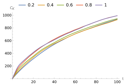
Figure 2: behaviour of $C_{K}(t)$ with level spacing

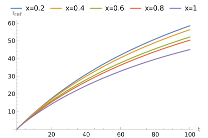
Figure 3: behaviour of $OQSL$ with level spacing

The initial linear growth of $b_{n}$ (Figure 1) decreases with the increase in repulsion level, which is followed by a brief plateau and descent. As the initial Lanczos coefficients determine the early behaviour of the K-complexity, the latter grows at faster rates in cases where level repulsion is minimal, see Figure 2. Since $O$ is not a local operator, the early linear growth of K-complexity cannot be associated with scrambling [53]. The OQSL (Figure 3) of the complexity operator increase with the increase in level repulsion.

Numerically, by analysing the Kernel of the super-operator $\mathbb{S}=[\mathcal{L},.]$ and the decomposition of $\mathcal{K}$ in the eigen-space of $\mathbb{S}$, we find that $\mathcal{I}$ is not the only stationary element under $e^{-i\mathcal{L}t}$ evolution. In other words, due to non-vanishing support of $|\mathcal{K})$ over $ker(\mathbb{S})$, the $QOSL$ is not tight for choice of $\mathcal{H}$ and $O$. This limit can be further refined by subtracting the projection of $|\mathcal{K})$ on $ker(\mathbb{S})$ from the $|\mathcal{K})$; for more details see [46].

We recall that the GOE does not represent generic physical systems, since all energy levels interact. Hence, it is more prudent to study $OQSL$ and K-complexity in many-body systems from integrable to chaotic regimes. This work will consider the ANNI [56, 57] Hamiltonian is a transverse field Ising chain with a non-integrable next-nearest-neighbour interaction term with open boundary conditions. The Hamiltonian for the model is

$$\mathcal{H}(g,h)=-\sum_{i=1}^{L}(Z_{i}Z_{i+1}+hX_{i}+gX_{i}X_{i+2}),$$ (13)

Since the ANNI model is non-integrable for $|g|>0$, it can only be handled numerically through exact diagonalisation. We study the behaviour of K-complexity and $OQSL$ as we change the integrability breaking parameter $g>0$. Due to the tensor product structure of the Hamiltonian, the $OQSL$ and K-complexity will depend on the initial operator $O$ and its tensor product structure. This behaviour was absent in the previous case, as the eigenvectors of matrices drawn from the GOE are random.

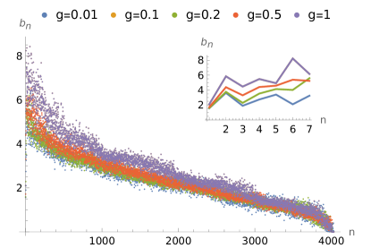
Figure 4: behaviour of $b_{n}$ with integrability breaking parameter $g$. Inset shows $b_{n}$ for small $n$.

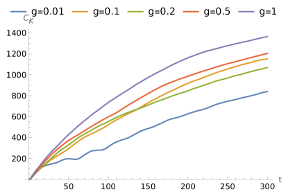
Figure 5: behaviour of $C_{K}(t)$ with integrability breaking parameter $g$.

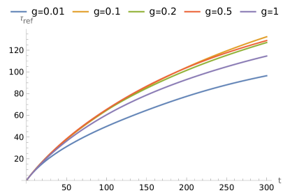
Figure 6: behaviour of $OQSL$ with integrability breaking parameter $g$.

The OQSL (Figure 6) initially increases with the integrability breaking term $g$ and then decreases as $g$ increases. A key difference in the behaviour of $b_{n}$ ( 4) from the RMT case is the presence of an early rise in $b_{n}$ even for $g=1$, which is absent in the RMT $x=1$ case although both of these lie in chaotic regimes. This is due to the local structure of $O$ which propotional to ($7X_{L/2}$ + $4Z_{L/2}$ ) and $\mathcal{H}$. There will always be initial spreading of the local operator irrespective of the integrability of $\mathcal{H}$. In Figure 5, the complexity grows at faster rates for higher values of $g$, which is expected as the $b_{n}$ grows faster with $n$. This behaviour is in contrast with the RMT case. Similar to the RMT case, this OQSL is not tight for the ANNI model, and we expect this to be the case for generic finite many-body systems.

Overall, the OQSL of the complexity operator is determined by the spectrum of $\mathbb{S}$ and the projection of $\mathcal{K}$ on the eigenbases of $\mathbb{S}$. However, due to the tensor product structure of the many-body Hamiltonian, it is worthwhile to study the Krylov basis operators $|K_{n})$ in a different operator basis that recognises the local structure of both $\mathcal{H}$ and $O$. This allows us to comment on the structure of the Krylov operators from an information-theoretic point of view.

IV Entanglement and Scrambling in Krylov space

According to the resource theory of scrambling [50, 51, 52], the mechanisms by which quantum information becomes scrambled can be categorized into two distinct classes: entanglement scrambling and Magic scrambling Figure 7. In entanglement scrambling, local Pauli operators, which initially affect only a tiny, localized part of the quantum system, evolve into Pauli operators of larger weight. This process spreads quantum information across a broader system region, increasing the entanglement and making it more challenging to extract the information without reversing the entire dynamics of the many-body system. Non-entangling unitaries do not increase the Pauli operators’ weight; under conjugation, they take weight-1 Pauli operators to weight-1 Pauli operators.

On the other hand, Magic scrambling involves transforming a few Pauli operators into a complex superposition of many different Pauli operators. The “magic” of the quantum state refers to the non-stabilizer nature of quantum states that cannot be efficiently simulated by classical means. In this case, free unitary transformation (Clifford unitaries) on the Pauli operators preserves their structure, changing only the phase factor, but not creating a superposition of multiple Pauli operators. Magic scrambling of a non-clifford unitary is quantified by the distance between the unitary and the set of Clifford unitaries, identical to the resource theory of Magic [58].

These distinctions highlight how local quantum information spreads and is rendered inaccessible, contributing to our understanding of quantum chaos and the dynamics of complex quantum systems.

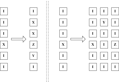
Figure 7: Left - Entanglement Scrambling due to an increase in the size of the string of Pauli operators, Right- Magic Scrambling due to mapping of Pauli operators into superposition of multiple operators. Figure inspired from [50]

IV.1 Influence and Coherence in Krylov Operator space

This section studies the influence and coherence of the time-evolved operator $O(t)$ and the Krylov basis operators $|K_{n})$ generated during the Lanczos algorithm. We start with the generalised n-qubit Pauli group as $\mathcal{P}^{\otimes n}_{2}=\{P_{\vec{a}}:P_{\vec{a}}=\otimes^{n}_{i=1}P_{a_{i}}\}_{\vec{a}\in\mathbb{V}_{2}^{n}}$ with $P_{a_{i}}=X^{s_{i}}Z^{t_{i}}$ and $a_{i}=(s_{i},t_{i})\in\mathbb{V}_{2}=\mathbb{Z}_{2}\otimes\mathbb{Z}_{2}$. $X$ and $Z$ are Pauli $Z$ and $X$ operators respectively. In this basis, it is natural to work with the inner product $\big{<}O_{1},O_{2}\big{>}\equiv\frac{Tr(O_{1}^{\dagger}O_{2})}{2^{n}}$ which is just the Hilbert Schmidt product normalised by the dimension of the Hilbert space. Any $n$-qubit operator $O$ can now be written as $O=\sum_{\vec{a}\in\mathbb{V}_{2}^{n}}c_{\vec{a}}P_{\vec{a}}$ with $c_{\vec{a}}={\big{<}O,P_{\vec{a}}\big{>}}$. The normalisation condition $\sqrt{\big{<}O,O\big{>}}=1$ implies $\sum_{\vec{a}\in\mathbb{V}_{2}^{n}}|c_{\vec{a}}|^{2}=1$.

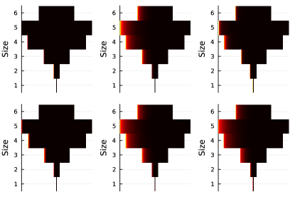
Figure 8: behaviour of $|c_{\vec{a}}|$ for different Krylov basis operators $n=\{6,500,4000\}$ for $g=0.01$ (top row) and $g=0.5$ (bottom row) .

To visualize both scrambling mechanisms, we plot the elements $|c_{\vec{a}}|$ via density plots, where each row represents the projection of the operator $O$ on operators of a fixed size. The elements in each row correspond to all the Pauli basis elements of a particular size $|\vec{a}|$. Here, the size $|\vec{a}|$ is defined by the number of non-identity operators in the basis element $P_{\vec{a}}$. For instance, a Pauli basis element with size $|\vec{a}|=2$ might include operators like $X\otimes I\otimes Z$ or $I\otimes Y\otimes X$. The density plot thus provides a visual representation of how the operator $O$ is projected onto these basis elements of varying sizes, highlighting the distribution of its components. In this visualization, snapshots of Krylov basis operators show similar patterns for small and intermediate values of $n$ (e.g., $n=6$ and $n=500$). This similarity suggests that the scrambling dynamics are relatively the same across this $n$.

However, for a large $n=4000$, the pattern changes significantly depending on the coupling constant $g$. When $g=0.5$, the Krylov operator is spread over many high-weight operators, indicating extensive scrambling where the operator has components across many basis elements, each with many non-identity terms. In contrast, when $g=0.01$, only a few high-weight operators primarily support the Krylov operator. This behaviour suggests that the operator exhibits less magic scrambling with smaller values of $g$, meaning that it has not diffused as broadly across the operator basis. This reduction in scrambling implies that the system’s evolution allows for some unscrambling of initial quantum information. Overall, this density plot analysis shows how the complexity and distribution of the operator $O$ change under different levels of integrability breaking.

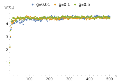
Figure 9: behaviour of $W(K_{n})$ integrability breaking parameter $g$.

Now, the average size of an operator $O$ can be quantified by its influence [21, 50].

$$W(O)=\sum_{\vec{a}\in\mathbb{V}_{2}^{n}}|\vec{a}||c_{\vec{a}}|^{2}$$ (14)

Influence is the average number (size) of non-Identity operator in the Pauli - basis expansion of $O$. Another valuable metric for assessing the spread of $O$ in the Pauli basis is the inverse participation ratio (IPR), given by $\frac{1}{\sum_{\vec{a}}|c_{\vec{a}}|^{4}}$, [59, 60]. This ratio provides effective basis elements over which the operator $O(t)$ has significant support. The IPR captures how coherently the operator $O$ is distributed across the Pauli operator basis. A low IPR indicates that $O$ is concentrated in the few basis elements, suggesting a less scrambled operator. Conversely, a high IPR signifies that $O$ is spread out over many basis elements, reflecting higher scrambling and complexity. This metric serves as a measure of the coherence of $O$ with respect to the Pauli basis. By analyzing the IPR, we can gain insights into the degree to which $O$ has evolved, and how its components are distributed, providing a clearer picture of the operator’s dynamics in the quantum system.

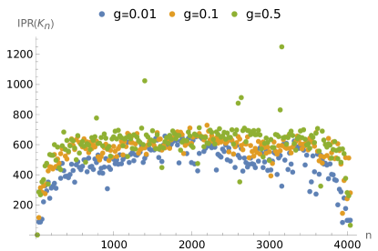
Figure 10: behaviour of $IPR(K_{n})$ with integrability breaking parameter $g$.

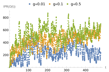
Figure 11: behaviour $IPR(O(t))$ with integrability breaking parameter $g$.

For a unitary to function effectively as a magic scrambler, it must also be proficient in entanglement scrambling. Because the number of available operators to form a superposition increases dramatically as the size of the operator string increases. Therefore, examining the operator’s influence and coherence is instructive for determining whether the dynamics generate entanglement and magic scrambling.

In Figure 9, we observe that the influence of the initial Krylov basis operators increases and then saturates for all subsequent Krylov basis operators, regardless of the value of $g$. It suggests that quantum chaos does not play a significant role in the influence dynamic of the operator. In contrast, the inverse participation ratio of the Krylov basis operators $\big{|}K_{n}\big{)}$ and the time-evolved operator $\big{|}O(t)\big{)}$ exhibits distinct behaviours for different values of the integrability breaking parameter $g$. For a small $g=0.01$, the IPR of $\big{|}K_{n}\big{)}$ peaks at central values of $n$, indicating that the operator is most coherent and localized in these regions, which suggests limited magic scrambling. However, for larger values of $g=0.1$ and $g=0.5$, the IPR shows a plateau-like behaviour, implying that the operator is spread more uniformly across many basis elements. This distribution suggests more magic scrambling as the operator forms superpositions over a more extensive set of basis elements. By analyzing both the influence and the IPR—we can see how the system’s dynamics facilitate entanglement and magic scrambling. This dual capability is essential for complex quantum systems to act as an effective scrambler of quantum information.

IV.2 Operator Entanglement

This section examines the operator entanglement entropy (OpEE) of the time-evolved operator $O(t)$ [49, 61, 62] and the Krylov basis operators generated during the Lanczos algorithm. To define the OpEE, we consider a bipartition of the spin chain into two subsystems, $\mathbb{A}$ and $\mathbb{B}$. Similar to the previous section, we can construct two separate bases for each of these subsystems, consisting of $(n_{\mathbb{A}},n_{\mathbb{B}})$ qubits, respectively. The basis vectors for these subsystems can be written as $A_{\vec{a}}=\otimes_{i=1}^{n_{\mathbb{A}}}P_{a_{i}}$, where $\vec{a}\in\mathbb{V}^{n_{\mathbb{A}}}_{2}$, and $B_{\vec{b}}=\otimes_{i=1}^{n_{\mathbb{B}}}P_{b_{i}}$, where $\vec{b}\in\mathbb{V}^{n_{\mathbb{B}}}_{2}$. Any operator $O$ can be decomposed uniquely $O=\sum_{\vec{a}\in\mathbb{V}^{n_{\mathbb{A}}}_{2},\vec{b}\in\mathbb{V}^{n_{\mathbb{B}}}_{2}}O_{\vec{a},\vec{b}}A_{\vec{a}}\otimes B_{\vec{b}}$ where $O_{\vec{a},\vec{b}}=\big{<}A_{\vec{a}}\otimes B_{\vec{b}}\big{|}O\big{>}$. Now the OpEE of the normalised operator $O$ with $\sqrt{\big{<}O,O\big{>}}=1$ can be defined as

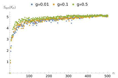
Figure 12: behaviour of $S_{en}$ of $K_{n}$ with integrability breaking parameter $g$.

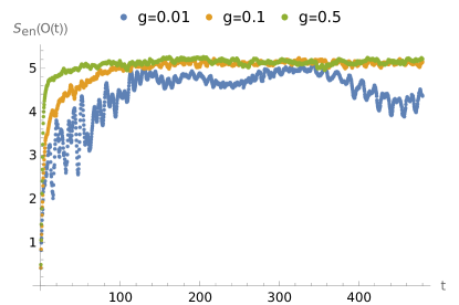
Figure 13: behaviour of $S_{en}$ of $O(t)$ with integrability breaking parameter $g$.

$$S_{en}=-Tr(\rho^{\mathbb{A}}_{op}log(2,\rho^{\mathbb{A}}_{op}))~{},$$ (15)

where $(\rho^{\mathbb{A}}_{op})_{\vec{a},\vec{a^{\prime}}}=\sum_{\vec{b}\in\mathbb{V}^{n_{\mathbb{B}}}_{2}}O_{\vec{a},\vec{b}}O^{\dagger}_{\vec{b},\vec{a^{\prime}}}$.

In Figure 13, the operator entanglement entropy (OpEE) of the initial $\big{|}K_{n}\big{)}$ exhibits varying growth patterns for different values of $g$. As the integrability-breaking perturbation increases, the OpEE saturates more rapidly, increasing $n$. However, regardless of the values of $g$, the OpEE of higher $\big{|}K_{n}\big{)}$ remains saturated, indicating a stabilization of entanglement in Krylov basis operators. This behaviour contrasts with the OpEE of $O(t)$, which never saturates even at late times for lower values of $g$.

V Discussions

We explored the relationship between the operator quantum speed limit of the complexity operator $\mathcal{K}$ and level-repulsion in both random/integrable matrices and many-body systems. In the case of random/integrable matrices, we observed that the OQSL increases with the level repulsion, whereas the growth rate of K-complexity decreases. This indicates a correlation between the repulsion of energy levels and the speed at which the complexity operator can evolve. The decrease in the growth rate of K-complexity might be an artefact of taking eigenvectors of $\mathcal{H}(x)$ as random vectors for every value of $x$.

In many-body systems, the behaviour is more complicated due to the presence of the tensor product structure. Initially, the OQSL increases with the integrability-breaking parameter $g$, suggesting that breaking integrability allows for faster evolution of the complexity operator. However, at larger values of$g$, the OQSL decreases, indicating a slowdown in the operator’s evolution speed.

Contrary to the random/integrable case, the growth rate of K-complexity in many-body systems rises with increasing $g$. This suggests that as integrability is further broken, the complexity of the operators grows faster in many-body dynamics.

For systems exhibiting chaotic dynamics, the Krylov operator $\big{|}K_{n}\big{)}$ remains a reliable representation of the coherence and entanglement properties of the time-evolved operator $O(t)$ even for moderate values of $n$, particularly at late times. This reliability comes from the complex nature of chaotic dynamics, which tend to spread $O(t)$ across all basis elements, leading to significant entanglement and scrambling.

The coherence of Krylov basis operators shows distinct behaviour for integrable dynamics, making it a better probe for chaos than opEE. The reliability is lacking when dealing with the entanglement dynamics. In integrable systems, the dynamics is more constrained, leading to limited spreading of $O(t)$ and reduced entanglement. As a result, the Krylov operator $\big{|}K_{n}\big{)}$ may fail to accurately capture the entanglement exhibited by the time-evolved operator $O(t)$, especially during late times.

This distinction highlights the crucial role of chaotic dynamics in generating extensive entanglement and scrambling. In contrast, integrable dynamics impose constraints that can limit the ability of certain representations, such as the Krylov operator, to faithfully reflect the actual entanglement dynamics of the system.

Acknowledgements

We sincerely thank Kunal Pal and Kuntal Pal for discussions. The work of TS is supported in part by the USV Chair Professor position at the Indian Institute of Technology, Kanpur.

References

- Bohigas et al. [1984] O. Bohigas, M. J. Giannoni, and C. Schmit, Characterization of chaotic quantum spectra and universality of level fluctuation laws, Phys. Rev. Lett. 52, 1 (1984).
- Berry and Tabor [1977] M. V. Berry and M. Tabor, Level Clustering in the Regular Spectrum, Proceedings of the Royal Society of London Series A 356, 375 (1977).
- Peres [1984] A. Peres, Stability of quantum motion in chaotic and regular systems, Phys. Rev. A 30, 1610 (1984).
- von Keyserlingk et al. [2018] C. von Keyserlingk, T. Rakovszky, F. Pollmann, and S. Sondhi, Operator hydrodynamics, OTOCs, and entanglement growth in systems without conservation laws, Phys. Rev. X 8, 021013 (2018), arXiv:1705.08910 [cond-mat.str-el] .
- Maldacena et al. [2016] J. Maldacena, S. H. Shenker, and D. Stanford, A bound on chaos, JHEP 08, 106, arXiv:1503.01409 [hep-th] .
- Kitaev [2015] A. Kitaev, A simple model of quantum holography (part 1) (2015).
- Srednicki [1994] M. Srednicki, Chaos and quantum thermalization, Phys. Rev. E 50, 888 (1994).
- Deutsch [1991] J. M. Deutsch, Quantum statistical mechanics in a closed system, Phys. Rev. A 43, 2046 (1991).
- Rigol et al. [2008] M. Rigol, V. Dunjko, and M. Olshanii, Thermalization and its mechanism for generic isolated quantum systems, Nature 452, 854 (2008), arXiv:0708.1324 [cond-mat.stat-mech] .
- D’Alessio et al. [2016] L. D’Alessio, Y. Kafri, A. Polkovnikov, and M. Rigol, From quantum chaos and eigenstate thermalization to statistical mechanics and thermodynamics, Adv. Phys. 65, 239 (2016), arXiv:1509.06411 [cond-mat.stat-mech] .
- Swingle et al. [2016] B. Swingle, G. Bentsen, M. Schleier-Smith, and P. Hayden, Measuring the scrambling of quantum information, Phys. Rev. A 94, 040302 (2016).
- Xu et al. [2020] T. Xu, T. Scaffidi, and X. Cao, Does scrambling equal chaos?, Phys. Rev. Lett. 124, 140602 (2020), arXiv:1912.11063 [cond-mat.stat-mech] .
- Sachdev and Ye [1993] S. Sachdev and J. Ye, Gapless spin-fluid ground state in a random quantum Heisenberg magnet, Phys. Rev. Lett. 70, 3339 (1993), arXiv:cond-mat/9212030 [cond-mat] .
- Maldacena and Stanford [2016] J. Maldacena and D. Stanford, Remarks on the Sachdev-Ye-Kitaev model, Phys. Rev. D 94, 106002 (2016), arXiv:1604.07818 [hep-th] .
- Dowling and Nielsen [2008] M. R. Dowling and M. A. Nielsen, The geometry of quantum computation, Quant. Inf. Comput. 8, 0861 (2008), arXiv:quant-ph/0701004 .
- Bhattacharyya et al. [2018] A. Bhattacharyya, A. Shekar, and A. Sinha, Circuit complexity in interacting QFTs and RG flows, JHEP 10, 140, arXiv:1808.03105 [hep-th] .
- Ali et al. [2019] T. Ali, A. Bhattacharyya, S. Shajidul Haque, E. H. Kim, and N. Moynihan, Time Evolution of Complexity: A Critique of Three Methods, JHEP 04, 087, arXiv:1810.02734 [hep-th] .
- Jaiswal et al. [2022] N. Jaiswal, M. Gautam, and T. Sarkar, Complexity, information geometry, and Loschmidt echo near quantum criticality, J. Stat. Mech. 2207, 073105 (2022), arXiv:2110.02099 [quant-ph] .
- Pal et al. [2023] K. Pal, K. Pal, A. Gill, and T. Sarkar, Evolution of circuit complexity in a harmonic chain under multiple quenches, J. Stat. Mech. 2305, 053108 (2023), arXiv:2206.03366 [quant-ph] .
- Brandão et al. [2021] F. G. S. L. Brandão, W. Chemissany, N. Hunter-Jones, R. Kueng, and J. Preskill, Models of Quantum Complexity Growth, PRX Quantum 2, 030316 (2021), arXiv:1912.04297 [hep-th] .
- Parker et al. [2019] D. E. Parker, X. Cao, A. Avdoshkin, T. Scaffidi, and E. Altman, A Universal Operator Growth Hypothesis, Phys. Rev. X 9, 041017 (2019), arXiv:1812.08657 [cond-mat.stat-mech] .
- Viswanath and Müller [2008] V. Viswanath and G. Müller, The Recursion Method: Applications to Many-body Dynamics, Lecture Notes in Physics Monographs (Springer Berlin, Heidelberg, 2008).
- Baggioli et al. [2024] M. Baggioli, K.-B. Huh, H.-S. Jeong, K.-Y. Kim, and J. F. Pedraza, Krylov complexity as an order parameter for quantum chaotic-integrable transitions, (2024), arXiv:2407.17054 [hep-th] .
- Nandy et al. [2024] P. Nandy, A. S. Matsoukas-Roubeas, P. Martínez-Azcona, A. Dymarsky, and A. del Campo, Quantum Dynamics in Krylov Space: Methods and Applications, (2024), arXiv:2405.09628 [quant-ph] .
- Chen et al. [2024] L. Chen, B. Mu, H. Wang, and P. Zhang, Dissecting Quantum Many-body Chaos in the Krylov Space, (2024), arXiv:2404.08207 [quant-ph] .
- Menzler and Jha [2024] H. G. Menzler and R. Jha, Krylov localization as a probe for ergodicity breaking, (2024), arXiv:2403.14384 [quant-ph] .
- Sasaki [2024] R. Sasaki, Towards Verifications of Krylov Complexity, PTEP 2024, 063A01 (2024), arXiv:2403.06391 [quant-ph] .
- Bhattacharya et al. [2024] A. Bhattacharya, P. P. Nath, and H. Sahu, Speed limits to the growth of Krylov complexity in open quantum systems, Phys. Rev. D 109, L121902 (2024), arXiv:2403.03584 [quant-ph] .
- Basu et al. [2024] R. Basu, A. Ganguly, S. Nath, and O. Parrikar, Complexity growth and the Krylov-Wigner function, JHEP 05, 264, arXiv:2402.13694 [hep-th] .
- Craps et al. [2024] B. Craps, O. Evnin, and G. Pascuzzi, A Relation between Krylov and Nielsen Complexity, Phys. Rev. Lett. 132, 160402 (2024), arXiv:2311.18401 [quant-ph] .
- Liu et al. [2023] C. Liu, H. Tang, and H. Zhai, Krylov complexity in open quantum systems, Phys. Rev. Res. 5, 033085 (2023), arXiv:2207.13603 [cond-mat.str-el] .
- Balasubramanian et al. [2022] V. Balasubramanian, P. Caputa, J. M. Magan, and Q. Wu, Quantum chaos and the complexity of spread of states, Phys. Rev. D 106, 046007 (2022), arXiv:2202.06957 [hep-th] .
- Nizami and Shrestha [2023] A. A. Nizami and A. W. Shrestha, Krylov construction and complexity for driven quantum systems, Phys. Rev. E 108, 054222 (2023), arXiv:2305.00256 [quant-ph] .
- Avdoshkin et al. [2024] A. Avdoshkin, A. Dymarsky, and M. Smolkin, Krylov complexity in quantum field theory, and beyond, Journal of High Energy Physics 2024, 66 (2024), arXiv:2212.14429 [hep-th] .
- Bhattacharyya et al. [2023] A. Bhattacharyya, S. S. Haque, G. Jafari, J. Murugan, and D. Rapotu, Krylov complexity and spectral form factor for noisy random matrix models, JHEP 10, 157, arXiv:2307.15495 [hep-th] .
- Jeevanesan [2023] B. Jeevanesan, Krylov Spread Complexity of Quantum-Walks, (2023), arXiv:2401.00526 [quant-ph] .
- Bhattacharjee [2023] B. Bhattacharjee, A Lanczos approach to the Adiabatic Gauge Potential, (2023), arXiv:2302.07228 [quant-ph] .
- Takahashi and del Campo [2024] K. Takahashi and A. del Campo, Shortcuts to Adiabaticity in Krylov Space, Phys. Rev. X 14, 011032 (2024), arXiv:2302.05460 [quant-ph] .
- Deffner and Campbell [2017] S. Deffner and S. Campbell, Quantum speed limits: from Heisenberg’s uncertainty principle to optimal quantum control, J. Phys. A 50, 453001 (2017), arXiv:1705.08023 [quant-ph] .
- Margolus and Levitin [1998] N. Margolus and L. B. Levitin, The Maximum speed of dynamical evolution, Physica D 120, 188 (1998), arXiv:quant-ph/9710043 .
- Eisert et al. [2015] J. Eisert, M. Friesdorf, and C. Gogolin, Quantum many-body systems out of equilibrium, Nature Phys. 11, 124 (2015), arXiv:1408.5148 [quant-ph] .
- Mandelstam and Tamm [1991] L. Mandelstam and I. Tamm, The uncertainty relation between energy and time in non-relativistic quantum mechanics, in Selected Papers (Springer Berlin Heidelberg, Berlin, Heidelberg, 1991) pp. 115–123.
- Lloyd [2000] S. Lloyd, Ultimate physical limits to computation, Nature 406, 1047 (2000).
- Nicholson et al. [2020] S. B. Nicholson, L. P. García-Pintos, A. del Campo, and J. R. Green, Time-information uncertainty relations in thermodynamics (2020), arXiv:2001.05418 [cond-mat.stat-mech] .
- Carabba et al. [2022] N. Carabba, N. Hörnedal, and A. del Campo, Quantum speed limits on operator flows and correlation functions, Quantum 6, 884 (2022), arXiv:2207.05769 [quant-ph] .
- Hörnedal et al. [2023] N. Hörnedal, N. Carabba, K. Takahashi, and A. del Campo, Geometric Operator Quantum Speed Limit, Wegner Hamiltonian Flow and Operator Growth, Quantum 7, 1055 (2023), arXiv:2301.04372 [quant-ph] .
- Hörnedal et al. [2022] N. Hörnedal, N. Carabba, A. S. Matsoukas-Roubeas, and A. del Campo, Ultimate Speed Limits to the Growth of Operator Complexity, Commun. Phys. 5, 207 (2022), arXiv:2202.05006 [quant-ph] .
- Scaramazza et al. [2016] J. A. Scaramazza, B. S. Shastry, and E. A. Yuzbashyan, Integrable matrix theory: Level statistics, Phys. Rev. E 94, 032106 (2016), arXiv:1604.01691 [cond-mat.mes-hall] .
- Wang and Zanardi [2002] X. Wang and P. Zanardi, Quantum entanglement of unitary operators on bipartite systems, Phys. Rev. A 66, 044303 (2002), arXiv:quant-ph/0207007 [quant-ph] .
- Garcia et al. [2023] R. J. Garcia, K. Bu, and A. Jaffe, Resource theory of quantum scrambling, Proc. Nat. Acad. Sci. 120, e2217031120 (2023), arXiv:2208.10477 [quant-ph] .
- Hayden and Preskill [2007] P. Hayden and J. Preskill, Black holes as mirrors: Quantum information in random subsystems, JHEP 09, 120, arXiv:0708.4025 [hep-th] .
- Shenker and Stanford [2014] S. H. Shenker and D. Stanford, Black holes and the butterfly effect, JHEP 03, 067, arXiv:1306.0622 [hep-th] .
- Rabinovici et al. [2021] E. Rabinovici, A. Sánchez-Garrido, R. Shir, and J. Sonner, Operator complexity: a journey to the edge of Krylov space, JHEP 06, 062, arXiv:2009.01862 [hep-th] .
- Rabinovici et al. [2022] E. Rabinovici, A. Sánchez-Garrido, R. Shir, and J. Sonner, Krylov localization and suppression of complexity, JHEP 03, 211, arXiv:2112.12128 [hep-th] .
- Hashimoto et al. [2023] K. Hashimoto, K. Murata, N. Tanahashi, and R. Watanabe, Krylov complexity and chaos in quantum mechanics, JHEP 11, 040, arXiv:2305.16669 [hep-th] .
- Selke [1988] W. Selke, The annni model — theoretical analysis and experimental application, Physics Reports 170, 213 (1988).
- S Suzuki [2012] B. K. C. S Suzuki, J Inoue, Quantum Ising Phases and Transitions in Transverse Ising Models, Lecture Notes in Physics (Springer Berlin, Heidelberg, 2012).
- Emerson et al. [2014] J. Emerson, D. Gottesman, S. A. H. Mousavian, and V. Veitch, The resource theory of stabilizer quantum computation, New J. Phys. 16, 013009 (2014), arXiv:1307.7171 [quant-ph] .
- Santos and Rigol [2010] L. F. Santos and M. Rigol, Onset of quantum chaos in one-dimensional bosonic and fermionic systems and its relation to thermalization, Phys. Rev. E 81, 036206 (2010).
- Anand et al. [2021] N. Anand, G. Styliaris, M. Kumari, and P. Zanardi, Quantum coherence as a signature of chaos, Phys. Rev. Res. 3, 023214 (2021), arXiv:2009.02760 [quant-ph] .
- Zhou and Luitz [2017] T. Zhou and D. J. Luitz, Operator entanglement entropy of the time evolution operator in chaotic systems, Phys. Rev. B 95, 094206 (2017), arXiv:1612.07327 [cond-mat.stat-mech] .
- Alba et al. [2019] V. Alba, J. Dubail, and M. Medenjak, Operator Entanglement in Interacting Integrable Quantum Systems: The Case of the Rule 54 Chain, Phys. Rev. Lett. 122, 250603 (2019), arXiv:1901.04521 [cond-mat.stat-mech] .