A Functional Central Limit Theorem for the
General Brownian Motion on the Half-Line

Abstract.

In this work, we establish a Trotter-Kato type theorem. More precisely, we characterize the convergence in distribution of Feller processes by examining the convergence of their generators. The main novelty lies in providing quantitative estimates in the vague topology at any fixed time. As important applications, we deduce functional central limit theorems for random walks on the positive integers with boundary conditions, which converge to Brownian motions on the positive half-line with boundary conditions at zero.

1. Introduction

The subject of functional central limit theorems (functional CLTs) originated from the now standard Donsker Theorem and Invariance Principles for Brownian motion. Since then, a substantial body of literature has emerged, focusing on invariance principles for various types of random walks (including those on random media) and their convergence to standard Brownian motion. However, the convergence to Brownian-type processes, such as the skew Brownian motion, sticky Brownian motion, elastic Brownian motion, and others, has received much less attention up to the present day.

As some rare examples, in 1981, Harrison and Lemoine [8] showed the convergence of a specific queue to sticky Brownian motion. In 1991, Amir [1] established the convergence of rescaled discrete-time random walks with deterministic waiting times, also to sticky Brownian motion. More recently, in 2021, Erhard, Franco, and da Silva [5] proved a functional central limit for the slow bond random walk. The limit of this process is given by the snapping out Brownian motion, a Brownian-type process created in 2016 by Lejay [11]. Somewhat related to the subject, in a recent paper [10], Kosygina, Mountford, and Peterson have shown the convergence of the one-dimensional cookie random walk (a walk that takes a decision based on the local time of the present position) towards what they called a Brownian motion perturbed at extrema, which is a stochastic process $W(t)$ solving a functional equation relating $W(t)$, its maxima and minima, and a standard Brownian motion.

In this work, we present a criterion to ensure a functional central limit theorem for Feller processes, based on the rate of convergence of their generators. This criterion comes with a corresponding Berry-Esseen type estimate. Convergence in distribution via the convergence of generators is not a new topic. A classical result in the book by Ethier and Kurtz [6, Theorem 6.1 on page 28] can be paraphrased as follows:

Consider a sequence $(T_{n})$ of strongly continuous contraction semigroups, where each $T_{n}$ is defined on a Banach space $\text{X}_{n}$ and has generator $L_{n}$. Denote by $\pi_{n}$ the projection of another Banach space X onto $\text{X}_{n}$ where a strongly continuous semigroup $T$ with generator $L$ is defined. Then $T_{n}(t)\pi_{n}f$ converges to $T(t)f$ for each $t$ if and only if for every $f$ in a core for $L$ there exists $f_{n}$ in a core for $L_{n}$ such that $f_{n}\to f$ and $L_{n}f_{n}\to Lf$. Our main result complements the above result and shows that a rate of convergence in the convergence of the generators implies a rate of convergence of the corresponding semigroups. This in turn will imply a rate of convergence in the vague topology of the law induced by $T_{n}$ to the one induced by $T$. Our result therefore establishes a sort of weak Berry-Esseen estimate. The primary applications we have in mind are boundary problems, where we show that, in many cases, it is crucial that the function $f_{n}$ does not necessarily coincide with $\pi_{n}f$ but can be chosen to address issues arising from the boundary conditions. As an interesting application of this general framework, we establish a functional central limit theorem for a wide class of random walks on the positive integers, which converge to the most general Brownian motion on the positive half-line.

The most general Brownian motion on the positive half-line was studied by Feller, and a comprehensive overview on it can be found in Knight’s book, see [9, Theorem 6.2, p. 157]. To put it simply, it is defined as a class of Feller processes on the positive half line such that its excursion to zero are the same as those of a standard Brownian motion, which can shown to be a mixture of the reflected Brownian motion, absorbed Brownian motion, and killed Brownian motion. Its generator is given by one half of the continuous Laplacian acting on the domain of ${\mathcal{C}}^{2}$-functions decaying at infinity and satisfying $c_{1}f(0)-c_{2}f^{\prime}(0)+\frac{c_{3}}{2}f^{\prime\prime}(0)=0$ with $c_{1}+c_{2}+c_{3}=1$, $c_{i}\geq 0$. Given three non-negative parameters $c_{1},c_{2},c_{3}$ that sum to one, we also occasionally denote by $B(c_{1},c_{2},c_{3})$ the corresponding general Brownian motion.

The discrete class of models considered here involves continuous-time random walks on $(\frac{1}{N}\mathbb{N})\cup\{\Delta\}$, where $\mathbb{N}={0,1,\ldots}$ and the state $\Delta$ is usually referred to as the cemetery. The walk follows the usual symmetric walk on ${1,2,\ldots}$ with jump rates to nearest neighbors everywhere equal to $1/2$. However, at state $0$, we introduce the following: the rate to jump to state $1$ is $A/n^{\alpha}$, and the rate to jump to the cemetery is $B/n^{\beta}$, where $\alpha,A,\beta,B\geq 0$, and $n$ is the scaling parameter. Additionally, if the walk reaches the cemetery, it remains there indefinitely.

The chosen values of parameters $\alpha,A,\beta,B$ then determine the limitingBrownian-type process of the random walk. We show here that for any choice of $c_{1},c_{2},c_{3}\geq 0$ such that $c_{1}+c_{2}+c_{3}=1$ and $c_{1}\neq 1$ there are classes of choices of $\alpha,A,\beta,B$ such that the above random walk converges to $B(c_{1},c_{2},c_{3})$. We additionally show that by making a small shift to the right of the random walk, we have convergence to the killed Brownian motion, which corresponds to $c_{1}=1$.

Each type of Brownian motion has different properties and behaviors, which makes them useful in different applications. For example, reflected Brownian motion can model a financial asset that cannot have negative values, while absorbed Brownian motion can model the extinction of a biological population. Elastic Brownian motion can model the behavior of a particle that is attracted to $0$ but has long-range repulsion from some boundary point and finally, the sticky Brownian motion can model a particle that sticks to a point, the killed Brownian motion corresponds to a continuous walk that jumps directly to the cemetery when it gets arbitrarily close to the origin. All these processes are particular cases of the above-mentioned general Brownian motion on the half-line, which illustrates the importance of the functional central limit theorem we prove in this paper. Moreover, the speed of convergence here obtained can come in handy when simulating those processes. Indeed, the random walks considered can be easily simulated as we will show in Section 4.

The outline of the paper is the following: in Section 2 we state results and mention related literature. Proofs are given in Section 3. Finally, Section 4 is dedicated to computational simulations of the simple random walk with boundary conditions which, by the presented results, are good approximations of the general BM on the half-line.

2. Statement of results

We use the convention that the set of natural numbers starts at zero, i.e., ${\mathbb{N}}=\{0,1,\ldots\}$. Throughout this paper, for given functions $f$ and $g$, the notation $f\lesssim g$ indicates the existence of a constant $c>0$ such that $f(n)\leq cg(n)$ for all $n\in\mathbb{N}$. The constant $c$ is independent of $n\in{\mathbb{N}}$ but is allowed to depend on other parameters.

2.1. The setup

For each $n\in{\mathbb{N}}$, consider strongly continuous contraction semigroups $\{T_{n}(t):t\geq 0\}$ and $\{T(t):t\geq 0\}$ acting on Banach spaces ${\mathsf{B}}_{n}$ and ${\mathsf{B}}$, with generators ${\mathsf{L}}_{n}$ and ${\mathsf{L}}$, respectively. We denote the domains of ${\mathsf{L}}$ and ${\mathsf{L}}_{n}$ by ${\mathfrak{D}}({\mathsf{L}})$ and ${\mathfrak{D}}({\mathsf{L}}_{n})$. To keep the notation simple, all norms are denoted by $\left\lVert\cdot\right\rVert$.

Let $\pi_{n}:{\mathsf{B}}\to{\mathsf{B}}_{n}$ be bounded linear operators indexed by $n\in{\mathbb{N}}$, which we call natural projections for reasons that will become clear in the sequel.

Let $\Xi_{n}:{\mathsf{B}}\to{\mathsf{B}}_{n}$ be a bounded family of linear operators, which we call the correction operators. Denote by $\left\lVert\cdot\right\rVert_{\text{op}}$ the operator norm. We further denote

$$\Phi_{n}\;=\;\pi_{n}+\Xi_{n}\,.$$ (2.1)

The following hypotheses will be crucial in this work. Here, by $f\in{\mathfrak{D}}({\mathsf{L}}^{2})$ we mean that $f\in{\mathfrak{D}}({\mathsf{L}})$ and ${\mathsf{L}}f\in{\mathfrak{D}}({\mathsf{L}})$.

1. If $f\in{\mathsf{B}}$, then $\Phi_{n}f\in{\mathfrak{D}}({\mathsf{L}_{n}})$.

2. There exist sequences $s_{1}(n)\searrow 0$, $s_{2}(n)\searrow 0$ and $s_{3}(n)\searrow 0$ such that, for any $f\in{\mathfrak{D}}({\mathsf{L}}^{2})$,

   $$\left\lVert\pi_{n}{\mathsf{L}}f-{\mathsf{L}}_{n}\Phi_{n}f\right\rVert\;\leq\;s_{1}(n)\left\lVert f\right\rVert+s_{2}(n)\left\lVert{\mathsf{L}}f\right\rVert+s_{3}(n)\left\lVert{\mathsf{L}}^{2}f\right\rVert\,.$$

3. There exist sequences $r_{1}(n)\searrow 0$ and $r_{2}(n)\searrow 0$ such that, for each $f\in{\mathfrak{D}}({\mathsf{L}}^{2})$,

   $$\left\lVert\Xi_{n}f\right\rVert\;\leq\;r_{1}(n)\left\lVert f\right\rVert+r_{2}(n)\left\lVert{\mathsf{L}}f\right\rVert\,.$$

As we see next, these conditions yield a bound on the distance between the semi-groups generated by ${\mathsf{L}}_{n}$ and ${\mathsf{L}}$. This is a quantitative version of [6, Thm 6.1, p. 28], attributed to Sova and Kurtz, which is sometimes referred to in the literature as Trotter-Kato Theorem.

Theorem 2.1.

Under hypotheses (H1) – (H3), for any $f\in{\mathfrak{D}}({\mathsf{L}}^{2})$ and for each $t\geq 0$ in a compact interval $[a,b]$ we have that

$$\left\lVert{T}_{n}(t)\pi_{n}f-\pi_{n}T(t)f\right\rVert\;\lesssim\; \max\left\{s_{1}(n),r_{1}(n)\right\}\left\lVert f\right\rVert+\max\big{\{}s_{2}(n),r_{1}(n),r_{2}(n)\big{\}}\left\lVert{\mathsf{L}}f\right\rVert$$

$$+\max\big{\{}s_{3}(n),r_{2}(n)\big{\}}\left\lVert{\mathsf{L}}^{2}f\right\rVert\,.$$

Here, the proportionality constant depends only on $b$.

Now we restrict ourselves to the setup of probability measures.

Let $({\mathsf{S}},d)$ be a separable locally compact (but possibly not complete) metric space. By $\lim_{x\to\infty}f(x)=0$ we mean that

$$\lim_{x:\,d(x,x_{0})\to\infty}f(x)\;=\;0$$ (2.2)

for some fixed point $x_{0}\in{\mathsf{S}}$. Note that the particular choice of $x_{0}$ is not relevant. Denote by $\overline{S}$ the completion of the metric space $({\mathsf{S}},d)$ with respect to the metric $d$ and denote also $\partial{\mathsf{S}}=\overline{S}\backslash S$.

If ${\mathsf{S}}$ is not complete (i.e. $\partial{\mathsf{S}}\neq\varnothing$), denote by $\Delta$ the set $\partial{\mathsf{S}}$, which we treat as a single point, and for $u\in{\mathsf{S}}$, we define $d(u,\Delta):=\inf\{d(u,v):v\in\partial{\mathsf{S}}\}$.

If ${\mathsf{S}}$ is complete (i.e. $\partial{\mathsf{S}}=\varnothing$), denote by $\Delta$ an extra point isolated from ${\mathsf{S}}$. That is, the distance of $\Delta$ to any point of ${\mathsf{S}}$ is, let’s say, at least one.

Definition 2.2.

Let ${\mathcal{C}}_{0}({\mathsf{S}})$ be the space of continuous functions $f:{\mathsf{S}}\cup\{\Delta\}\to\mathbb{R}$ such that the two conditions below hold:

• $\displaystyle\lim_{x\to\infty}f(x)=0$,

• $f(\Delta)=0$.

Note that if $\partial{\mathsf{S}}$ is not empty, then the continuity implies that

$$\lim_{x\to x_{0}}f(x)\;=\;0\,,\quad\text{ for any }x_{0}\in\partial{\mathsf{S}}.$$

The point $\Delta$ above defined is called the cemetery. We state below our next hypotheses:

1. The Banach space ${\mathsf{B}}$ is given by ${\mathcal{C}}_{0}({\mathsf{S}})$ equipped with the uniform topology and the natural projection $\pi_{n}$ is the restriction to a subset ${\mathsf{S}}_{n}$ of ${\mathsf{S}}$, that is, $\pi_{n}f=f|_{{\mathsf{S}}_{n}}$.

2. There is a sequence of functions $\{f_{k}\}_{k\geq 0}$ in ${\mathcal{C}}_{0}({\mathsf{S}})$ such that $\operatorname{span}(\{f_{k}\})$ is dense. Moreover, for each $k\in{\mathbb{N}}$, there exists a sequence of functions $\{f_{k,j}:j\geq 0\}\subset{\mathfrak{D}}({\mathsf{L}}^{2})$ such that $f_{k,j}\to f_{k}$ when $j\to\infty$, in the uniform topology (in particular, the set ${\mathfrak{D}}({\mathsf{L}}^{2})$ is dense in ${\mathcal{C}}_{0}({\mathsf{S}})$).

3. It holds that, for all $k,j\geq 0$,

   $$\left\lVert{\mathsf{L}}f_{k,j}\right\rVert\;\leq\;h_{1}(j)\left\lVert f_{k}\right\rVert\quad\text{ and }\quad\left\lVert{\mathsf{L}}^{2}f_{k,j}\right\rVert\;\leq\;h_{2}(j)\left\lVert f_{k}\right\rVert\,,$$ (2.3)

   where the sequences $h_{1}(j)$ and $h_{2}(j)$ satisfy

   $$\sum_{j\geq 0}\frac{h_{i}(j)}{2^{j}}<\infty\,,\quad i=1,2.$$ (2.4)

   Moreover, it holds that

   $$\sum_{k\geq 0}\frac{\left\lVert f_{k}\right\rVert}{2^{k}}<\infty\,.$$ (2.5)

   and

   $$\sum_{j,k\geq 0}\frac{\left\lVert f_{k,j}\right\rVert}{2^{k+j}}<\infty\,.$$ (2.6)

4. The semigroup ${\mathsf{T}}$ associated to the generator ${\mathsf{L}}$ is Lipschitz in the sense that, for each $t>0$, there exists a constant $M=M(t)>0$ such that

   $$|{\mathsf{T}}(t)f(x)-{\mathsf{T}}(t)f(y)|\;\leq\;M\cdot\|f\|\cdot d(x,y)\,,\quad\forall\,x,y\in{\mathsf{S}}\,.$$

   for all $f\in{\mathsf{B}}={\mathcal{C}}_{0}({\mathsf{S}})$.

Remark 2.3.

Note that in (2.3) the functions $h_{1}$ and $h_{2}$ do not depend on $k$, and in this sense (2.3) is uniform in $k\in{\mathbb{N}}$. Moreover, the technical condition (2.5) tells us that the norm of $f_{k}$ does not grows too fast. The key point here is to insure that $\operatorname{span}(\{f_{k}\})$ is dense. In particular, by normalizing the functions $f_{k}$ we can always guarantee that (2.5) holds. Finally, (2.6) is of course a consequence of (2.5), (2.3), and (2.4). However, stating it here simplifies our presentation later on.

We now introduce a suitable distance on the space of sub-probability measures that implies vague convergence. Let ${\mathcal{B}}$ be the Borel $\sigma$-algebra on $({\mathsf{S}},d)$ and let ${\mathcal{M}}_{\leq 1}(S)$ be the set of sub-probability measures over the measurable space $({\mathsf{S}},{\mathcal{B}})$.

Definition 2.4.

Let $\{f_{k}\}_{k\geq 0}\subset{\mathcal{C}}_{0}({\mathsf{S}})$ and $\{f_{k,j}:j\geq 0\}\subset{\mathfrak{D}}({\mathsf{L}}^{2})$ be as in (G2). We define

$${\bf d}(\mu,\nu)\;:=\;\sum_{j,k=0}^{\infty}\frac{1}{2^{k+j}}\left(\bigg{|}\int f_{k,j}\text{\rm d}\mu-\int f_{k,j}\text{\rm d}\nu\bigg{|}\wedge 1\right)$$

for any $\mu,\nu\in{\mathcal{M}}_{\leq 1}(S)$.

At a first glance, it may seem odd to define the distance ${\bf d}$ in terms of a double indexed sequence $\{f_{k,j}\}$ instead of a single indexed sequence, as it is usually done. We use the above notation since it will be more natural for our applications. We also highlight the fact that each $f_{k,j}$ is in the domain of ${\mathsf{L}}^{2}$, which will be crucial for the arguments to come.

The next proposition is a straightforward consequence of the definitions of vague and weak convergence, and for this reason we omit its proof.

Proposition 2.5.

The function ${\bf d}:{\mathcal{M}}_{\leq 1}({\mathsf{S}})\times{\mathcal{M}}_{\leq 1}({\mathsf{S}})\to[0,+\infty)$ defined in Definition 2.4 is a metric on the set ${\mathcal{M}}_{\leq 1}({\mathsf{S}})$ and convergence with respect to the metric $\bf d$ is equivalent to vague convergence. Moreover, if $\lim_{n\to\infty}{\bf d}(\mu_{n},\mu)=0$ and $\mu$ is a probability measure, then $\mu_{n}$ converges weakly to $\mu$.

We are in a position to state the first main result of this work. Recall that ${\mathsf{S}}_{n}\subset{\mathsf{S}}$.

Theorem 2.6 (Berry-Esseen estimate with respect to ${\bf d}$ and functional CLT).

Assume hypotheses (H1)–(H3) and (G1)–(G4). Let $\big{\{}X(t):t\in[0,T]\big{\}}$ and $\big{\{}X_{n}(t):t\in[0,T]\big{\}}$ be the Feller processes on ${\mathsf{S}}$ and ${\mathsf{S}}_{n}$ associated to the generators ${\mathsf{L}}$ and ${\mathsf{L}}_{n}$, respectively, assumed to start at the points $x_{n}\in{\mathsf{S}_{n}}$ and $x\in{\mathsf{S}}$, respectively, where $d(x_{n},x)\leq i(n)$ for some function $i(n)$.

Fix some time $t>0$ and denote by $\mu$ and $\mu_{n}$ the probability distributions on ${\mathsf{S}}$ induced by $X(t)$ and $X_{n}(t)$, respectively, starting from the points $x_{n}\in{\mathsf{S}}_{n}$ and $x\in{\mathsf{S}}$. Then

$${\bf d}(\mu,\mu_{n})\;\lesssim\;\max\big{\{}i(n),s_{1}(n),s_{2}(n),s_{3}(n),r_{1}(n),r_{2}(n)\big{\}}\,.$$ (2.7)

Moreover, we also have pathwise convergence $X_{n}\Rightarrow X$ in the Skorohod space${\mathsf{D}}_{{\mathsf{S}}}[0,\infty)$.

Remark 2.7.

The main novelty in the statement above is the weak Berry-Esseen estimate (2.7). The convergence in the Skorohod space ${\mathsf{D}}_{{\mathsf{S}}}[0,\infty)$ is actually a corollary of (2.7) and [6, Theorem 2.11, page 172].

2.2. Application to the general Brownian motion on ${\mathbb{R}}_{\geq 0}$

We apply Theorem 2.1 in order to obtain a Donsker-type theorem for what is known in the literature as the general Brownian motion on the half line. To that end, let us first define it. We denote by $B_{0}(t)$ the Brownian motion on $[0,\infty)$ absorbed upon reaching zero. We use $\Delta$ to represent the cemetery state, and we let $T_{0}$ be the hitting time of zero.

Definition 2.8 ([9], p. 153).

A general Brownian motion on the positive half-line is a diffusion process $W$ on the set ${\mathbb{G}}:=\{\Delta\}\cup[0,\infty)$ such that the absorbed process $\{W(t\wedge T_{0}):t\geq 0\}$ on $[0,\infty)$ has the same distribution as $B_{0}$ for any starting point $x\geq 0$.

Theorem 2.9 (Feller, see [9], Theorem 6.2, p. 157).

Any general Brownian motion $W$ on $[0,\infty)$ has generator ${\mathsf{L}}=\frac{1}{2}\frac{d^{2}}{dx^{2}}$ with corresponding domain

$${\mathfrak{D}}\big{(}{\mathsf{L}}\big{)}=\Big{\{}f\,\in\,{\mathcal{C}}_{0}^{2}({\mathbb{G}})\,:f^{\prime\prime}\in{\mathcal{C}}_{0}({\mathbb{[}0,\infty)})\,\text{ and }c_{1}f(0)-c_{2}f^{\prime}(0)+\frac{c_{3}}{2}f^{\prime\prime}(0)=0\Big{\}}$$ (2.8)

for some $c_{i}\geq 0$ such that $c_{1}+c_{2}+c_{3}=1$ and $c_{1}\neq 1$.

Figure 1. Description of the general Brownian motion on the half-line according to the chosen values of $c_{1},c_{2},c_{3}\geq 0$ on the simplex $c_{1}+c_{2}+c_{3}=1$. Note that the killed BM, which formally corresponds to $c_{1}=1$, is not rigorously a case of the general BM, as we can see in Theorem 2.9.

We will now discuss the above process.

The case $c_{2}=1$ corresponds to the reflected Brownian motion (which has the distribution of the modulus of an standard BM), while $c_{3}=1$ yields the absorbed Brownian motion, which has the distribution of a standard BM stopped at zero.

As one can see above, the case $c_{1}=1$ is not part of Feller’s Theorem 2.9, which imposes $c_{1}\neq 1$. Indeed, for $c_{1}=1$ the domain (2.8) is not a dense set in ${\mathcal{C}}_{0}({\mathbb{G}})$, where ${\mathbb{G}}=\{\Delta\}\cup[0,\infty)$ so it cannot be a domain of a generator. But once we remove the origin, considering ${\mathbb{G}}=\{\Delta\}\cup(0,\infty)$ instead, it will define a Feller process because now the set of test functions is assumed to converge to zero at the origin (c.f. Definition 2.2 and refer to [4, Chapter 2] for details). The killed BM can be understood as the process which jumps immediately to the cemetery $\Delta$ upon “reaching the origin”. Actually, it never touches the origin, but gets arbitrarily close, which explains why $c_{1}=1$ is not included in Theorem 2.9: since the killed BM does not touch zero, it cannot satisfy the condition of Definition 2.8. Despite the absorbed BM and killed BM being different processes, they are similar in nature, and to improve the presentation we will freely consider the killed BM as being a particular case of the general BM on the positive half-line.

The case $c_{1}=0$ corresponds to the sticky Brownian motion, which is an interpolation between the absorbed BM and the reflected BM, spending a time of positive Lebesgue measure at zero (but not staying there for any non degenerated time interval). See [2, 12] on the subject, for example.

The case $c_{3}=0$ corresponds to the elastic BM (also called partially reflected Brownian motion) which it is a mixture of the reflected BM and killed BM. It can be also constructed in terms of the local time at zero: we toss an exponential random variable $\tau$ (whose parameter is related to $c_{1}$ and $c_{2}$) and a path of the reflected BM. Once the local time at zero of the reflected BM reaches the value $\tau$, the process goes to the cemetery and stays there forever (see [11] and references therein).

The case $c_{2}=0$ corresponds to the exponential holding BM. Its behavior is the following: once it visits zero, it stays there for an exponentially distributed amount of time and then is killed (jumps to the cemetery and stays there forever). See [9] on the exponential holding BM. This case allows us to interpret the case $c_{1}=1$ as a kind of explosion: it is an extreme case of the exponential holding BM, where the parameter of the exponential clock associated to jumps from the origin to the cemetery is infinite, leading to an instantaneous jump.

The case $c_{1},c_{2},c_{3}>0$ is a mixture of these behaviours, and we will refer to any such process as the mixed BM. Finally, it is instructive to mention that there are actually only two behaviours at zero. Namely, how much the BM sticks at zero, and how much the BM is attracted to the cemetery. This is in agreement with the fact that there are three parameters $c_{1}$, $c_{2}$ and $c_{3}$, but only two degrees of freedom, since those parameters are restricted to the simplex $c_{1}+c_{2}+c_{3}=1$. See Figure 1 for an illustration of the general BM in terms of the choices of $c_{1}$, $c_{2}$ and $c_{3}$.

Next we define a random walk on the non-negative integers that, as we shall see, is a discrete version of the general BM on the positive half-line.

Figure 2. Jump rates for the boundary random walk.

The boundary random walk is the the Feller process depending on parameters $A,B,\alpha,\beta\geq 0$ and $n\in{\mathbb{N}}$ on the state space ${\mathbb{G}}_{n}:=\big{(}\frac{1}{n}{\mathbb{N}}\big{)}\cup\{\Delta\}$, whose generator $\mathsf{L}_{n}$ acts on functions $f:\mathbb{G}_{n}\to{\mathbb{R}}$ as follows:

$${\mathsf{L}}_{n}f(x)=\begin{cases}\dfrac{1}{2}\Big{[}f\big{(}x+\genfrac{}{}{}{1}{1}{n}\big{)}-f(x)\Big{]}+\dfrac{1}{2}\Big{[}f\big{(}x-\genfrac{}{}{}{1}{1}{n}\big{)}-f(x)\Big{]}\,,\;x=\genfrac{}{}{}{1}{1}{n},\genfrac{}{}{}{1}{2}{n},\ldots\vskip 12.0pt plus 4.0pt minus 4.0pt\\ \dfrac{A}{n^{\alpha}}\Big{[}f\big{(}\Delta\big{)}-f(\frac{0}{n})\Big{]}+\dfrac{B}{n^{\beta}}\Big{[}f\big{(}\genfrac{}{}{}{1}{1}{n}\big{)}-f\big{(}\genfrac{}{}{}{1}{0}{n}\big{)}\Big{]}\,,\quad\text{ for }x=\genfrac{}{}{}{1}{0}{n}\,.\end{cases}$$ (2.9)

The next result is our second main result, and as we will see follows from Theorem 2.6. The different cases stated below are illustrated in Figure 3.

Theorem 2.10 (Functional CLT for the boundary random walk).

Fix $u,t>0$. Let $\{X_{n}(t):t\geq 0\}$ be the boundary random walk of parameters $\alpha,\beta,A,B\geq 0$ sped up by $n^{2}$ (that is, whose generator is $n^{2}{\mathsf{L}}_{n}$), starting from the point $\frac{\lfloor un\rfloor}{n}\in{\mathbb{G}}_{n}\subset{\mathbb{G}}$ and denote by $\mu_{n}=\mu_{n}(t)$ the distribution of $X_{n}$ at time $t>0$. Recall the metric ${\bf d}$ defined in (2.7) and denote by $\mu=\mu(t)$ the distribution at time $t>0$ of the limit process in each of following cases. Then:

1. If $\alpha=\beta+1$ and $\beta\in[0,1)$, then $\{X_{n}(t):t\geq 0\}$ converges weakly to $\{X^{\text{EBM}}(t):t\geq 0\}$ in the $J_{1}$-Skorohod topology of ${\mathsf{D}}_{{\mathbb{G}}}[0,\infty)$, where $X^{\text{EBM}}$ is the elastic BM on ${\mathbb{G}}=\{\Delta\}\cup{\mathbb{R}}_{\geq 0}$ of parameters

   $$c_{1}=\frac{B}{A+B},\quad c_{2}=\frac{A}{A+B}\quad\text{ and }\quad c_{3}=0$$

   starting from the point $u$. Moreover,

   1. if $\beta\in(0,1)$, then ${\bf d}(\mu_{n},\mu)\lesssim\max\{n^{-\beta},n^{\beta-1}\}$ ,

   2. if $\beta=0$, then ${\bf d}(\mu_{n},\mu)\lesssim n^{-1}$ .

2. If $\alpha\in(2,+\infty]$ and $\beta=1$, then $\{X_{n}(t):t\geq 0\}$ converges weakly to $\{X^{\text{SBM}}(t):t\geq 0\}$ in the $J_{1}$-Skorohod topology of ${\mathsf{D}}_{{\mathbb{G}}}[0,\infty)$, where $X^{\text{SBM}}$ is the sticky BM on ${\mathbb{R}}_{\geq 0}$ of parameters

   $$c_{1}=0,\quad c_{2}=\frac{B}{B+1},\quad\text{ and }\quad c_{3}=\frac{1}{B+1}$$

   starting from the point $u$. Moreover, in this case,

   $${\bf d}(\mu_{n},\mu)\;\lesssim\;\max\{n^{2-\alpha},n^{-1}\}\,.$$

3. If $\alpha=2$ and $\beta\in(1,+\infty]$, then $\{X_{n}(t):t\geq 0\}$ converges weakly to $\{X^{\text{EHBM}}(t):t\geq 0\}$ in the $J_{1}$-Skorohod topology of ${\mathsf{D}}_{\mathbb{G}}[0,\infty)$, where $X^{\text{EHBM}}$ is the exponential holding BM on ${\mathbb{G}}=\{\Delta\}\cup{\mathbb{R}}_{\geq 0}$ of parameters

   $$c_{1}=\frac{A}{1+A},\quad c_{2}=0\quad\text{ and }\quad c_{3}=\frac{1}{1+A}$$

   starting from the point $u$. Moreover, for $\beta\in(2,\infty)$,

   $${\bf d}(\mu_{n},\mu)\;\lesssim\;\max\{n^{2-\beta},n^{-1}\}\,.$$

4. If $\alpha>\beta+1$ and $\beta\in[0,1)$, then $\{X_{n}(t):t\geq 0\}$ converges weakly to $\{X^{\text{RBM}}(t):t\geq 0\}$ in the $J_{1}$-Skorohod topology of ${\mathsf{D}}_{{\mathbb{R}}_{\geq 0}}[0,\infty)$, where $X^{\text{RBM}}$ is the reflected BM on ${\mathbb{R}}_{\geq 0}$, of parameters

   $$c_{1}=0,\quad c_{2}=1\quad\text{ and }\quad c_{3}=0$$

   starting from the point $u$. Moreover, for $\beta\in(0,1)$,

   1. if $1+\beta<\alpha<2$, then ${\bf d}(\mu_{n},\mu)\lesssim\max\{n^{-\beta},n^{-\alpha+\beta+1},n^{\alpha-2}\}\,,$

   2. if $\alpha=2$, then ${\bf d}(\mu_{n},\mu)\lesssim\max\{n^{-\beta},n^{\beta-1}\}$ ,

   3. if $\alpha>2$, then ${\bf d}(\mu_{n},\mu)\lesssim\max\{n^{2-\alpha},n^{-\beta},n^{\beta-1}\}$ .

5. If $\alpha\in(2,\infty]$ and $\beta\in(1,+\infty]$, then $\{X_{n}(t):t\geq 0\}$ converges weakly to $\{X^{\text{ABM}}(t):t\geq 0\}$ in the $J_{1}$-Skorohod topology of ${\mathsf{D}}_{{\mathbb{R}}_{\geq 0}}[0,\infty)$, where $X^{\text{ABM}}$ is the absorbed BM on ${\mathbb{R}}_{\geq 0}$, of parameters

   $$c_{1}=0,\quad c_{2}=0\quad\text{ and }\quad c_{3}=1$$

   starting from the point $u$. Moreover, for $\alpha>2$ and $\beta>2$,

   $${\bf d}(\mu_{n},\mu)\;\lesssim\;\max\{n^{2-\alpha},n^{2-\beta},n^{-1}\}\,.$$

6. If $\alpha=2$ and $\beta=1$, then $\{X_{n}(t):t\geq 0\}$ converges weakly to $\{X^{\text{MBM}}(t):t\geq 0\}$ in the $J_{1}$-Skorohod topology of ${\mathsf{D}}_{\mathbb{G}}[0,\infty)$, where $X^{\text{MBM}}$ is the mixed BM on ${\mathbb{G}}=\{\Delta\}\cup{\mathbb{R}}_{\geq 0}$ of parameters

   $$c_{1}=\frac{A}{1+A+B},\quad c_{2}=\frac{B}{1+A+B}\quad\text{ and }\quad c_{3}=\frac{1}{1+A+B}$$

   starting from the point $u$. Moreover, ${\bf d}(\mu_{n},\mu)\lesssim n^{-1}$.

Figure 3. Possible limits for the boundary random walk according to the ranges of $\alpha,\beta\in[0,\infty]$. Note that it includes the cases where $\alpha=\infty$ or $\beta=\infty$, which correspond to $A=0$ and $B=0$ respectively. Speed of convergence is provided for all choices of $\alpha$ and $\beta$, except for the strip $1<\beta<2$.

Since the natural state space of the killed BM is ${\mathbb{G}}=\{\Delta\}\cup(0,\infty)$, which does not include the origin, we need a different setup to have the convergence of the boundary random walk towards the killed BM. This is the content of the next result. Let $\tau_{n}:{\mathbb{G}}\to{\mathbb{G}}$ be the shift to the right of $1/n$ given by

$$\tau_{n}(\Delta)=\Delta\quad\text{ and }\quad\tau_{n}(u)=u+\genfrac{}{}{}{1}{1}{n}\quad\text{ for }u\in[0,\infty)\,.$$

Theorem 2.11 (Convergence of the shifted boundary RW to the killed BM).

If $\alpha<1+\beta$ for $\beta\in[0,1]$, or $\beta>1$, then $\{\tau_{n}X_{n}(t):t\geq 0\}$ converges weakly to $\{X^{\text{KBM}}(t):t\geq 0\}$ in the $J_{1}$-Skorohod topology of ${\mathsf{D}}_{\mathbb{G}}[0,\infty)$, where in this case $X^{\text{KBM}}$ is the killed BM on ${\mathbb{G}}=\{\Delta\}\cup(0,+\infty)$, which is formally the general BM of parameters

$$c_{1}=1,\quad c_{2}=0\quad\text{ and }\quad c_{3}=0\,.$$

3. Proofs

3.1. Proofs of Theorem 2.1 and Theorem 2.6

We start with the proof of Theorem 2.1.

Proof of Theorem 2.1.

Putting together hypotheses (H2) and (H3), we can infer that

$$\left\lVert\Phi_{n}{\mathsf{L}}f-{\mathsf{L}}_{n}\Phi_{n}f\right\rVert\, \leq\,s_{1}(n)\left\lVert f\right\rVert+2\max\{s_{2}(n),r_{1}(n)\}\left\lVert{\mathsf{L}}f\right\rVert$$

$$\qquad+2\max\{s_{3}(n),r_{2}(n)\}\left\lVert{\mathsf{L}}^{2}f\right\rVert\,,$$ (3.1)

for any $f\in{\mathfrak{D}}({\mathsf{L}}^{2})$. Fix $t\geq 0$ and define $g_{s,t}:={\mathsf{T}}(t-s)f$ for $0\leq s\leq t$. Then,

$$\partial_{s}g_{s,t}\;=\;\partial_{s}{\mathsf{T}}(t\,-\,s)f\;=\;-\,{\mathsf{L}}{\mathsf{T}(t\,-\,s)f\;=\;-\,{\mathsf{L}}g_{s,t}}.$$ (3.2)

Note that $\Phi_{n}f=\Phi_{n}g_{t,t}$. By (3.2) and the assumption that $\Phi_{n}$ is a bounded operator we obtain that

$${\mathsf{T}}_{n}(t)\Phi_{n}f\, =\,{\mathsf{T}}_{n}(0)\Phi_{n}g_{0,t}\,+\,\int_{0}^{t}\partial_{s}({\mathsf{T}}_{n}(s)\Phi_{n}g_{s,t})\,\text{\rm d}s$$

$$=\,{\mathsf{T}}_{n}(0)\Phi_{n}g_{0,t}\,+\,\int_{0}^{t}\big{[}{\mathsf{L}}_{n}{\mathsf{T}}_{n}(s)\Phi_{n}g_{s,t}\,-\,{\mathsf{T}}_{n}(s)\Phi_{n}{\mathsf{L}}g_{s,t}\big{]}\,\text{\rm d}s\,.$$

Using the equality above, using that semigroups are contractions, that $T_{n}(0)$ is the identity mapping and using that ${\mathsf{T}}(t){\mathsf{L}}={\mathsf{L}}{\mathsf{T}}(t)$ and ${\mathsf{T}}_{n}(t){\mathsf{L}}_{n}={\mathsf{L}}_{n}{\mathsf{T}}_{n}(t)$ for all $n\in{\mathbb{N}}$ and for all $t\geq 0$, we have that

$$\left\lVert{\mathsf{T}}_{n}(t)\Phi_{n}f-\Phi_{n}{\mathsf{T}}(t)f\right\rVert$$

$$=\;\left\lVert\int_{0}^{t}{\mathsf{T}}_{n}(s)\big{[}{\mathsf{L}}_{n}\Phi_{n}g_{s,t}-\Phi_{n}{\mathsf{L}}g_{s,t}\big{]}\,\text{\rm d}s\right\rVert$$

$$\leq\;\int_{0}^{t}\left\lVert{\mathsf{T}}_{n}\right\rVert_{\text{OP}}\cdot\left\lVert\big{[}{\mathsf{L}}_{n}\Phi_{n}g_{s,t}-\Phi_{n}{\mathsf{L}}g_{s,t}\big{]}\right\rVert\text{\rm d}s$$

$$\overset{\eqref{eq3.1}}{\leq}\;\int_{0}^{t}\Big{[}s_{1}(n)\left\lVert g_{s,t}\right\rVert+2\max\{s_{2}(n),\,r_{1}(n)\}\left\lVert{\mathsf{L}}g_{s,t}\right\rVert\Big{]}\,\text{\rm d}s$$

$$\qquad+\int_{0}^{t}2\max\{s_{3}(n),\,r_{2}(n)\}\left\lVert{\mathsf{L}}^{2}g_{s,t}\right\rVert\,\text{\rm d}s$$

$$=\!\int_{0}^{t}\Big{[}s_{1}(n)\left\lVert{\mathsf{T}}(t-s)f\right\rVert+2\max\{s_{2}(n),r_{1}(n)\}\left\lVert{\mathsf{L}}{\mathsf{T}}(t-s)f\right\rVert\Big{]}\text{\rm d}s$$

$$\qquad+2\int_{0}^{t}\max\{s_{3}(n),r_{2}(n)\}\left\lVert{\mathsf{L}}^{2}{\mathsf{T}}(t-s)f\right\rVert\,\text{\rm d}s$$

$$\leq\;2t\Big{(}s_{1}(n)\left\lVert f\right\rVert+\max\{s_{2}(n),\,r_{1}(n)\}\left\lVert{\mathsf{L}}f\right\rVert\Big{)}$$

$$\qquad\,+\,2t\max\{s_{3}(n),\,r_{2}(n)\}\left\lVert{\mathsf{L}}^{2}f\right\rVert\,,$$ (3.3)

for every $f\in{\mathfrak{D}}({\mathsf{L}}^{2})$. Note that hypothesis (H1) assures that ${\mathsf{L}}_{n}\Phi_{n}g_{s,t}$ above is well defined. Recall that $\Phi_{n}=\pi_{n}+\Xi_{n}$. By the triangle inequality,

$$\left\lVert{\mathsf{T}}_{n}(t)\pi_{n}f-\pi_{n}{\mathsf{T}}(t)f\right\rVert\, \leq\,\left\lVert{\mathsf{T}}_{n}(t)\Phi_{n}f-\Phi_{n}{\mathsf{T}}(t)f\right\rVert\,+\,\left\lVert{\mathsf{T}}_{n}(t)\Xi_{n}f\right\rVert\,+\,\left\lVert\Xi_{n}{\mathsf{T}}(t)f\right\rVert.$$

Invoking hypothesis (H3) and applying inequality (3.3) we conclude the proof. ∎

Proof of Theorem 2.6.

Let $\{f_{k}\}$ be a dense family in ${\mathcal{C}}_{0}({\mathsf{S}})$ and consider, for each fixed $k$, a sequence $f_{k,j}\subset{\mathfrak{D}}({\mathsf{L}}^{2})$ such that $f_{k,j}\to f_{k}$ in the uniform topology as in hypothesis (G2). For ease of notation, denote

$$a(n) =\max\{r_{1}(n),s_{1}(n)\}\,,$$

$$b(n) =\max\big{\{}s_{1}(n),r_{1}(n),r_{2}(n)\big{\}}\,,$$

$$c(n) =\max\big{\{}s_{2}(n),r_{2}(n)\big{\}}\,.$$

Thus

$${\bf d}(\mu_{n},\mu)=\;\sum_{k,j\geq 0}\frac{1}{2^{k+j}}\left(\left\lvert\int f_{k,j}\,\text{\rm d}\mu_{n}-\int f_{k,j}\,\text{\rm d}\mu\right\rvert\wedge 1\right)$$

$$\overset{\hyperlink{(G3),(G4) }{(G3),(G4)}}{\lesssim}\;\max\Big{\{}i(n),\sum_{k,j\geq 0}\frac{1}{2^{k+j}}\Big{(}\left\lVert{\mathsf{T}}_{n}(t)\pi_{n}f_{k,j}-\pi_{n}{\mathsf{T}}(t)f_{k,j}\right\rVert\wedge 1\Big{)}\Big{\}}$$

$$\overset{\text{Thm. }\ref{thm21}}{\lesssim}\;\max\Big{\{}i(n),\sum_{k,j\geq 0}\frac{1}{2^{k+j}}\Big{(}a(n)\left\lVert f_{k,j}\right\rVert+b(n)\left\lVert{\mathsf{L}}f_{k,j}\right\rVert+c(n)\left\lVert{\mathsf{L}}^{2}f_{k,j}\right\rVert\Big{)}\wedge 1\Big{\}}$$

$$\overset{\hyperlink{(G3)}{(G3)}}{\lesssim}\;\max\Big{\{}i(n),\sum_{k,j\geq 0}\frac{1}{2^{k+j}}\Big{(}a(n)\left\lVert f_{k}\right\rVert+b(n)h_{1}(j)\left\lVert f_{k}\right\rVert+c(n)h_{2}(j)\left\lVert f_{k}\right\rVert\Big{)}\wedge 1\Big{\}}$$

$$\overset{\hyperlink{(G3)}{(G3)}}{\lesssim}\max\big{\{}i(n),a(n),b(n),c(n)\big{\}}\,.$$

Here, the conditions (2.4) and (2.5) have been also used in the penultimate inequality, and (2.6) has been used in the first inequality. Finally, since $X_{n}(0)\Rightarrow X(0)$ and ${\bf d}(\mu_{n},\mu)\to 0$ as $n\to\infty$, by [6, Theorem 2.11, page 172] we conclude that $X_{n}\Rightarrow X$ in the Skorohod topology. ∎

3.2. Proof of Theorem 2.10

In order to prove Theorem 2.10, we will apply Theorem 2.6, so we must verify hypotheses (H1)–(H3) and (G1)–(G4).

We start with (G1)–(G3), whose arguments are general, afterwards we will deal with (H1)–(H3) and (G4), which require specific arguments for each choice of the parameters.

Hypothesis (G1) is immediate from the setup.

We come to hypotheses (G2) and (G3). We first construct the family $\{f_{k}\}_{k\geq 0}$. Recall that the domain of ${\mathsf{L}}$ is given by (2.8). To construct the desired families of functions we first define

$${\mathcal{A}}_{\geq 0}:=\Big{\{}p(x)e^{-x^{2}}:p:{\mathbb{R}}_{\geq 0}\to{\mathbb{R}}\text{ is a polynomial }\Big{\}}\,.$$

It is a well-known result that the linear vector space generated by ${\mathcal{A}}_{\geq 0}$ is dense in ${\mathcal{C}}_{0}({\mathbb{R}}_{\geq 0})$. However, we were not able to find a reference for that fact. For that reason we include a proof. Let

$${\mathcal{A}}:=\Big{\{}p(x)e^{-x^{2}}:p:{\mathbb{R}}\to{\mathbb{R}}\text{ is a polynomial }\Big{\}}\,.$$

Lemma 3.1.

The set $\operatorname{span}({\mathcal{A}})$ is dense in ${\mathcal{C}}_{0}({\mathbb{R}})$.

Proof.

Suppose by contradiction that $\operatorname{span}({\mathcal{A}})$ is not dense. Then, by the Hahn-Banach Theorem, there exists a non-zero functional ${\mathsf{\Lambda}}:{\mathcal{C}}_{0}({\mathbb{R}})\to{\mathbb{R}}$ such that ${\mathsf{\Lambda}}|_{\text{span}({\mathcal{A}})}\equiv 0$. By the Riesz-Markov Theorem, there exists a measure $\mu$ such that

$${\mathsf{\Lambda}}(f)\,:=\,\int f\,\text{\rm d}\mu$$

for all $f\in{\mathcal{C}}_{0}({\mathbb{R}})$. By the Jordan decomposition theorem, there exist $\mu^{+},\mu^{-}$ positive real-valued measures such that $\mu=\mu^{+}-\mu^{-}$ where at least one of the two measures is finite.

For any $g\in\text{span}({\mathcal{A}})$, it follows that $g(x)=p(x)e^{-x^{2}}$ for some polynomial $p$, and ${\mathsf{\Lambda}}(g)=0$. Thus

$$\int p(x)e^{-x^{2}}\,\text{\rm d}\mu^{+}\;=\;\int p(x)e^{-x^{2}}\,\text{\rm d}\mu^{-}\,.$$ (3.4)

Let $\nu^{+}(A)=\int_{A}e^{-x^{2}}\text{\rm d}\mu^{+}$ and $\nu^{-}(A)=\int_{A}e^{-x^{2}}\text{\rm d}\mu^{-}$ be real-valued measures, and define $\rho^{+},\rho^{-}:{\mathbb{C}}\to{\mathbb{R}}$ through $\rho^{\pm}(z):=\int e^{zx}\text{\rm d}\nu^{\pm}(x)$. Observe that $\rho^{\pm}$ are well-defined since

$$\left\lvert\int_{{\mathbb{R}}}e^{zx}\,\text{\rm d}\nu^{\pm}(x)\right\rvert\;=\;\left\lvert\int_{{\mathbb{R}}}e^{zx}e^{-x^{2}}\,\text{\rm d}\mu^{\pm}(x)\right\rvert\;\leq\;\int_{{\mathbb{R}}}\left\lvert e^{zx-x^{2}}\right\rvert\,\text{\rm d}\mu^{\pm}(x)<\infty\,.$$

To see that the last inequality is true, note that

$$\int e^{-x^{2}}\,\text{\rm d}\mu(x)\;=\;0\,.$$

Since either $\mu^{+}$ or $\mu^{-}$ are finite we can conclude that

$$\int e^{-x^{2}}\,\text{\rm d}\mu^{\pm}(x)\;<\;\infty\,,$$

from which the claim follows. In view of (3.4), we have that

$$\frac{d^{(n)}}{dz^{(n)}}\rho^{+}(0)\;=\;\frac{d^{(n)}}{dz^{(n)}}\rho^{-}(0)$$

which lead to, by comparison of its power series, that $\rho^{+}(z)=\rho^{-}(z)$ for any $z\in{\mathbb{C}}$. Therefore, for all $s\in{\mathbb{R}}$, $\rho^{+}(is)=\rho^{-}(is)$ for all $s\in{\mathbb{R}}$, and hence $\nu^{+}=\nu^{-}$, which guarantees that ${\mathsf{\Lambda}}\equiv 0$, a contradiction. Hence $\operatorname{span}({\mathcal{A}})$ must be dense in ${\mathcal{C}}_{0}({\mathbb{R}})$. ∎

As an immediate consequence of Lemma 3.1, we have

Corollary 3.2.

The set $\operatorname{span}({\mathcal{A}}_{\geq 0})$ is dense in ${\mathcal{C}}_{0}({\mathbb{R}}_{\geq 0})$.

Let $\tilde{f}_{k}:{\mathbb{R}}_{\geq 0}\to{\mathbb{R}}$ be defined by $\tilde{f}_{k}(x):=x^{k}e^{-x^{2}}$ for all $k\geq 0$, which are illustrated in Figure 4. By Corollary 3.2 we know that $\operatorname{span}(\{\widetilde{f}_{k}\}_{k\geq 0})$ is dense in ${\mathcal{C}}_{0}({\mathbb{R}}_{\geq 0})$ and an elementary calculation gives that $\|\widetilde{f}_{0}\|=1$ and $\|\widetilde{f}_{k}\|=\big{(}\genfrac{}{}{}{1}{k}{2}\big{)}^{\frac{k}{2}}e^{-\frac{k}{2}}$, for all $k\geq 1$. Then, the family of functions defined by

$$f_{k}\;:=\;\frac{\widetilde{f}_{k}}{\|\widetilde{f}_{k}\|}\,,\quad\forall\,k\geq 0\,,$$ (3.5)

still has the property that its span is dense in ${\mathcal{C}}_{0}({\mathbb{R}}_{\geq 0})$ and it satisfies (2.5).

Figure 4. Illustration of the functions $\widetilde{f}_{k}:{\mathbb{R}}_{\geq 0}\to{\mathbb{R}}$, $\widetilde{f}_{k}(x):=x^{k}e^{-x^{2}}$.

Our goal now is to find sequences $f_{k,j}\in{\mathfrak{D}}({\mathsf{L}}^{2})$ fulfilling hypotheses (G2) and (G3). Note that the functions $f_{k}$ are smooth and, for $k\geq 5$, the function itself and its first four derivatives at zero are zero. Recalling (2.8), this trivially implies that $f_{k}\in{\mathfrak{D}}({\mathsf{L}}^{2})$ for $k\geq 5$. Therefore, we define

$$f_{k,j}\;:=\;f_{k}\quad\text{ for }k\geq 5\,.$$

To treat the case $k\leq 4$, we define the shift operator $\tau_{j}$ by

$$\tau_{j}(f)(x)\;=\;f\Big{(}x-\frac{4}{j}\Big{)}\mathrm{\mathbf{1}}_{\left[x\geq\frac{4}{j}\right]}(x)\,.$$

Define now an extension of $\tau_{j}(f_{k})$ to the whole line through a reflection around the $y$-axis, that is,

$$g_{k,j}(x)\;:=\;\begin{cases}(\tau_{j})(f_{k})(x)\,,&\text{ if }x\geq 0\\ (\tau_{j})(f_{k})(-x)\,,&\text{ if }x<0\\ \end{cases}\quad\text{ for }k\in\{1,2,3,4\}\text{ and }j\geq 0\,,$$

which are continuous, but not smooth at the point $4/j$. To remedy this, consider the ${\mathcal{C}}^{\infty}$-approximation of identity $\varphi_{j}:{\mathbb{R}}\to{\mathbb{R}}$ given by

$$\varphi_{j}(x):=\begin{cases}\displaystyle\frac{1}{c_{j}}\exp{\left(-\frac{1}{1-(jx)^{2}}\right)}\,,&\text{ if }\left\lvert jx\right\rvert<1\vspace{5pt}\\ 0\,,&\text{ otherwise}\end{cases}$$

where

$$c_{j}:=\int_{{\mathbb{R}}}\exp{\Big{(}-\frac{1}{1-(jx)^{2}}\Big{)}}\mathds{1}_{\{|jx|\leq 1\}}\text{\rm d}x$$

is the normalizing constant. Note that $\varphi_{j}(x)=j\varphi_{1}(jx)$, which yields the following relation between the derivatives

$$\frac{d^{(i)}}{dx^{(i)}}\varphi_{j}(x)\;=\;j^{i+1}\frac{d^{(i)}}{dx^{(i)}}\varphi_{1}(jx)\,,\quad\forall\,j>0\,.$$ (3.6)

Define now

$$f_{k,j}(x)\;:=\;(g_{k,j}\ast\varphi_{j})(x)\quad\text{ for }k\in\{1,2,3,4\}\text{ and }j\geq 0\,,$$

which is smooth and a simple but tedious calculation shows that $f_{k,j}\to f_{k}$ uniformly as $j\to\infty$. Since in a neighborhood around zero, we obtain that $f_{k,j}\in{\mathfrak{D}}({\mathsf{L}}^{2})$ for any $k\in\{1,2,3,4\}$ and any $j\geq 0$.

Denote $\left\lVert\frac{d^{(i)}}{dx^{(i)}}\varphi_{1}\right\rVert=A_{i}$ for $i\in{\mathbb{N}}$. Observe that

$$\left|\frac{d^{(i)}}{dx^{(i)}}f_{k,j}(x)\right| \;=\;\left|\frac{d^{(i)}}{dx^{(i)}}\int_{-\frac{1}{j}}^{\frac{1}{j}}g_{k,j}(x-y)\varphi_{j}(y)\,dy\right|$$

$$\;=\;\left|\int_{-\frac{1}{j}}^{\frac{1}{j}}g_{k,j}(x-y)\frac{d^{(i)}}{dx^{(i)}}\varphi_{j}(y)dy\right|$$

$$\;\leq\;2j^{i}\left\lVert g_{k,j}\right\rVert A_{i}\,,$$

where we made use of the scaling relation (3.6) to obtain the last inequality. Since $\left\lVert g_{k,j}\right\rVert=\left\lVert f_{k}\right\rVert=1$, we obtain that

$$\left\lVert{\mathsf{L}}f_{k,j}\right\rVert\leq j^{2}A_{2}\quad\text{ and }\quad\left\lVert{\mathsf{L}}^{2}f_{k,j}\right\rVert\leq j^{4}A_{4}\,,\quad\forall\,k\geq 1,j\geq 0\,.$$

Now, it only remains to construct $f_{0,j}$ such that it verifies conditions (G2) and (G3). To that end, let ${\mathsf{P}}:{\mathbb{R}}_{\geq 0}\to{\mathbb{R}}$ be a polynomial such that both $e^{-x^{2}}+{\mathsf{P}}$ and $(e^{-x^{2}}+{\mathsf{P}})^{\prime\prime}$ satisfy the boundary condition (2.8) and such that additionally ${\mathsf{P}}(0)=0$. To continue, define the ${\mathcal{C}}^{\infty}$-bump function $b_{1}:{\mathbb{R}}\to{\mathbb{R}}_{\geq 0}$ by

$$b_{1}(t)\;=\;1-\frac{\ell(t^{2}-1)}{\ell(t^{2}-1)+\ell(2-t^{2})}$$

where

$$\ell(t)\;=\;\begin{cases}e^{-\frac{1}{t}},&\text{ if }t>0\\ 0,&\text{ if }t\leq 0\,,\end{cases}$$

and for $j\geq 1$ define $b_{j}(t)=b_{1}(jt)$. The function $0\leq b_{j}\leq 1$ is equal to one in an interval of size $1/j$ around the origin and zero outside the interval $[-\sqrt{2}/j,\sqrt{2}/j]$. Finally, define

$$f_{0,j}(x)\;:=\;e^{-x^{2}}+(b_{j}{\mathsf{P}})(x)\,.$$

The fact that $f_{0,j}$ vanishes for $x\geq\sqrt{2}/j$ and that $f_{0,j}(0)=1$ together with its continuity guarantee that $f_{0,j}\to e^{-x^{2}}$ as $j\to\infty$ in the uniform topology. Since the polynomial $e^{-x^{2}}+{\mathsf{P}}$ satisfies the aforementioned boundary condition, we also have $f_{0,j}\in{\mathfrak{D}}({\mathsf{L}}^{2})$ for all positive integers $j$. Note that $b_{j}(x)=b_{1}(jx)$, yielding for all $i\geq 0$ and all $j\geq 1$

$$\frac{d^{(i)}}{dx^{(i)}}b_{j}(x)\;=\;j^{i}\frac{d^{(i)}}{dx^{(i)}}b_{1}(jx)\,.$$

Since the generator of the general Brownian motion on the half-line is given by $\frac{1}{2}\Delta$, it is immediate that

$${\mathsf{L}}e^{-x^{2}}\;\lesssim\;x^{2}e^{-x^{2}}\quad\text{ and }\quad{\mathsf{L}}^{2}e^{-x^{2}}\;\lesssim\;x^{4}e^{-x^{2}}\,.$$ (3.7)

Now, since $b_{j}\equiv 0$ outside the compact set $[-\frac{\sqrt{2}}{j},\frac{\sqrt{2}}{j}]$ and ${\mathsf{P}}$ is a polynomial, for all $i\geq 1$ one has that $\left\lVert\frac{d^{(i)}}{dx^{(i)}}b_{j}{\mathsf{P}}\right\rVert\lesssim j^{i}$. Hence, using equation (3.7), the product rule and the bound above, we can obtain upper bounds for the generator ${\mathsf{L}}$ and ${\mathsf{L}}^{2}$ norm $\left\lVert{\mathsf{L}}f_{0,j}\right\rVert\lesssim\big{(}\left\lVert f_{2}\right\rVert+j^{2})\left\lVert f_{0}\right\rVert\lesssim j^{2}\left\lVert f_{0}\right\rVert$ and $\left\lVert{\mathsf{L}}^{2}f_{0,j}\right\rVert\lesssim\big{(}\left\lVert f_{4}\right\rVert+j^{4}\big{)}\left\lVert f_{0}\right\rVert\lesssim j^{4}\left\lVert f_{0}\right\rVert$, where we used that all the $f_{k}$’ s were normalized. Hence, we ensured that conditions (G2) and (G3) are met.

The Lipschitz hypothesis (G4) relies on the knowledge about the semigroup of the limiting process. The limiting processes mentioned in Theorem 2.10 are, the reflected, absorbed, mixed, stick, elastic, exponential holding and killed Brownian motion. All of them have explicit formulas for their semigroups (which are obtained from the semigroup of the standard Brownian motion), which can be found in the book [3, Appendix 1, starting at page 119]. From these formulas it can be checked that (G4) holds for each one of those semigroups. We omit these tedious calculations.

Remark 3.3.

Hypothesis (G4) has been used just once, in the proof of Theorem 2.6, and its importance relies on the fact that the random walk and its limiting process may not have the same starting point. For instance, in the setup of Theorem 2.10, the boundary random walk starts from $\lfloor un\rfloor/n$, whereas its Brownian counterpart starts from $u>0$. If we assume that the discrete process and the limiting process start from the same point $u\in{\mathsf{S}}$, hypothesis (G4) can be dropped from Theorem 2.6. This is possible in the setup of Theorem 2.10, for instance, if we assume that the scaling parameter is given by $n=n(k)=2^{k}$ and the initial point $u$ is a positive integer.

It therefore remains to verify the remaining assumptions. Those involve the correction operator $\Xi_{n}$, which is very model dependent. Before we study each model separately, we start with some generalities. We will always assume that $(\Xi_{n}f)(\Delta)=0$, and moreover all functions considered here satisfy $f(\Delta)=0$. Thus, the generator of the random walk with boundary conditions sped up by $n^{2}$, applied to the function $\Phi_{n}f$ at zero is given by

$$\begin{split}n^{2}{\mathsf{L}}_{n}\Phi_{n}f\big{(}\genfrac{}{}{}{1}{0}{n}\big{)}\;=\;&-\frac{A}{n^{\alpha-2}}f\big{(}\genfrac{}{}{}{1}{0}{n}\big{)}+\frac{B}{n^{\beta-2}}\left[f\big{(}\genfrac{}{}{}{1}{1}{n}\big{)}-f\big{(}\genfrac{}{}{}{1}{0}{n}\big{)}\right]\\ &-\frac{A}{n^{\alpha-2}}\Xi_{n}f(0)+\frac{B}{n^{\beta-2}}\left[\Xi_{n}f\big{(}\genfrac{}{}{}{1}{1}{n}\big{)}-\Xi_{n}f(0)\right]\,.\end{split}$$ (3.8)

Outside of zero, a Taylor expansion yields

$$n^{2}{\mathsf{L}}_{n}\Phi_{n}f\big{(}\genfrac{}{}{}{1}{x}{n}\big{)}\;=\; \frac{1}{2}\Delta f\big{(}\genfrac{}{}{}{1}{x}{n}\big{)}+\frac{1}{2\cdot 4!n^{2}}\left[f^{{}^{\prime\prime\prime\prime}}(\theta)+f^{{}^{\prime\prime\prime\prime}}(\eta)\right]$$

$$+\frac{n^{2}}{2}\Big{[}\Xi_{n}f\big{(}\genfrac{}{}{}{1}{x+1}{n}\big{)}+\Xi_{n}f\big{(}\genfrac{}{}{}{1}{x-1}{n}\big{)}-2\Xi_{n}f\big{(}\genfrac{}{}{}{1}{x}{n}\big{)}\Big{]}$$

$$\;=\; \frac{1}{2}\pi_{n}\Delta f\big{(}\genfrac{}{}{}{1}{x}{n}\big{)}+\|\Delta^{2}f\|\cdot O(n^{-2})+n^{2}{\mathsf{L}}_{n}\Xi_{n}f\big{(}\genfrac{}{}{}{1}{x}{n}\big{)}\,,$$ (3.9)

for some $\theta\in(x/n,(x+1)/n)$ and $\xi\in((x-1)/n,x/n)$.

3.3. The elastic BM: the case $\beta\in[0,1),\alpha=\beta+1$

Recall that in this case we set

$$c_{1}=\frac{B}{A+B},\quad c_{2}=\frac{A}{A+B}\quad\text{ and }\quad c_{3}=0\,.$$

Denote the generator of the elastic Brownian motion by ${\mathsf{L}}_{\text{EBM}}$. Its domain is given by

$${\mathfrak{D}}\left({\mathsf{L}}_{\text{EBM}}\right)\;=\;\left\{f\,\in\,{\mathcal{C}}_{0}^{2}({\mathbb{G}})\,:\,\frac{A}{A+B}f(0)\,-\,\frac{B}{A+B}f^{\prime}(0)\;=\;0\right\}.$$

Let $f\in{\mathfrak{D}}({\mathsf{L}}^{2}_{\text{EBM}})$, which yields the boundary conditions $Af(0)=Bf^{\prime}(0)$ and $Af^{\prime\prime}(0)=Bf^{\prime\prime\prime}(0)$. Using this together with $\alpha=1+\beta$ in Equation (3.8) together with a Taylor expansion, yields that

$$n^{2}{\mathsf{L}}_{n}\Phi_{n}f\big{(}\genfrac{}{}{}{1}{0}{n}\big{)}\;=\; -\frac{A}{n^{\alpha-2}}f\big{(}\genfrac{}{}{}{1}{0}{n}\big{)}+\frac{B}{n^{\beta-2}}\left[\frac{f^{\prime}(0)}{n}+\frac{f^{\prime\prime}(0)}{2!n^{2}}+\frac{f^{\prime\prime\prime}(0)}{3!n^{3}}+\frac{f^{\prime\prime\prime\prime}(\eta)}{4!n^{4}}\right]$$

$$-\frac{A}{n^{\alpha-2}}\Xi_{n}f(0)+\frac{B}{n^{\beta-2}}\Big{[}\Xi_{n}f\big{(}\genfrac{}{}{}{1}{1}{n}\big{)}-\Xi_{n}f(0)\Big{]}$$

$$\;=\; \frac{B}{n^{\beta}}\left[\frac{f^{\prime\prime}(0)}{2!}+\frac{A}{B}\frac{f^{\prime\prime}(0)}{3!n}+\frac{f^{\prime\prime\prime\prime}(\eta)}{4!n^{2}}\right]$$ (3.10)

$$-\frac{A}{n^{\beta-1}}\Xi_{n}f(0)+\frac{B}{n^{\beta-2}}\Big{[}\Xi_{n}f\big{(}\genfrac{}{}{}{1}{1}{n}\big{)}-\Xi_{n}f(0)\Big{]}$$ (3.11)

for some $0\leq\eta\leq 1/n$. Note that for $\beta>0$ the parcel (3.10) is vanishing, and it is at this point where the correction operator enters the game. Assume first that $\beta\neq 0$; we will discuss the situation $\beta=0$ at the ending of this subsection. Define

$$\Xi_{n}f\big{(}\genfrac{}{}{}{1}{x}{n}\big{)}\;:=\;-\frac{\frac{1}{2}f^{\prime\prime}(0)}{An^{1-\beta}\left(1+\frac{1}{n}g\left(\frac{x}{n}\right)\right)}\,,$$ (3.12)

where $g$ is some arbitrary nonnegative Lipschitz function of constant $K>0$ satisfying $g(0)=0$ and $g(u)\to\infty$ as $u\to\infty$. Note that the condition on the growth of $g$ is only necessary to assure that $\Xi_{n}$ belongs to the domain of ${\mathsf{L}}_{n}$ which is given by ${\mathfrak{D}}({\mathsf{L}}_{n})=\big{\{}f:\{\Delta\}\cup\genfrac{}{}{}{1}{1}{n}{\mathbb{N}}\to{\mathbb{R}}\text{ such that }\lim_{\frac{x}{n}\to\infty}f\big{(}\genfrac{}{}{}{1}{x}{n}\big{)}=0\text{ and }f(\Delta)=0\big{\}}$. We then have that

$$-\frac{A}{n^{\beta-1}} \Xi_{n}f(0)+\frac{B}{n^{\beta-2}}\Big{[}\Xi_{n}f\big{(}\genfrac{}{}{}{1}{1}{n}\big{)}-\Xi_{n}f(0)\Big{]}$$

$$=\frac{1}{2}f^{\prime\prime}(0)+\frac{Bn}{A}\left[\frac{\frac{1}{n}g\left(\frac{1}{n}\right)}{1+\frac{1}{n}g\left(\frac{1}{n}\right)}\right]\frac{1}{2}f^{\prime\prime}(0)$$

$$=\;{\mathsf{L}}_{\text{EBM}}f(0)+\frac{BK}{A}\|{\mathsf{L}}_{\text{EBM}}f\|\cdot O(n^{-1})$$

because $g(0)=0$ and $g$ is $K$-Lipschitz. Plugging it into (3.10) – (3.11) yields

$$\left|\left(\pi_{n}{\mathsf{L}}_{\text{EBM}}f-n^{2}{\mathsf{L}}_{n}\Phi_{n}f\right)(0)\right|\,\lesssim\,\left(\frac{1}{n^{\beta}}+\frac{1}{n}+\frac{1}{n^{1+\beta}}\right)\left\lVert{\mathsf{L}}_{\text{EBM}}f\right\rVert+\frac{1}{n^{2+\beta}}\left\lVert{\mathsf{L}}^{2}_{\text{EBM}}f\right\rVert\,.$$ (3.13)

For $\frac{x}{n}\in{\mathbb{G}}_{n}\backslash\{0\}$, equation (3.9) indicates that we need to estimate

$$n^{2}{\mathsf{L}}_{n}\Xi_{n}f\big{(}\genfrac{}{}{}{1}{x}{n}\big{)}$$

$$=\frac{{\mathsf{L}}_{\text{EBM}}f(0)n^{2}}{An^{1-\beta}}\left[\frac{\frac{1}{n}\left(g\big{(}\genfrac{}{}{}{1}{x+1}{n}\big{)}-g\big{(}\genfrac{}{}{}{1}{x}{n}\big{)}\right)}{\left(1+\frac{1}{n}g\left(\frac{x+1}{n}\right)\right)\left(1+\frac{1}{n}g\left(\frac{x}{n}\right)\right)}+\frac{\frac{1}{n}\left(g\left(\frac{x-1}{n}\right)-g\left(\frac{x}{n}\right)\right)}{\left(1+\frac{1}{n}g\left(\frac{x-1}{n}\right)\right)\left(1+\frac{1}{n}g\left(\frac{x}{n}\right)\right)}\right]$$

$$=K\|{\mathsf{L}}_{\text{EBM}}\|O(n^{\beta-1})\,,$$

where we used again that $g$ is $K$-Lipschitz. Plugging it into (3.9), we conclude that

$$\left|\left(\pi_{n}{\mathsf{L}}_{\text{EBM}}f-n^{2}{\mathsf{L}}_{n}\Phi_{n}f\right)\big{(}\genfrac{}{}{}{1}{x}{n}\big{)}\right|\;\lesssim\;\frac{1}{n^{1-\beta}}\left\lVert{\mathsf{L}}_{\text{EBM}}f\right\rVert+\frac{1}{n^{2}}\left\lVert{\mathsf{L}}^{2}_{\text{EBM}}f\right\rVert$$ (3.14)

uniformly in $\frac{x}{n}\in{\mathbb{G}}_{n}\backslash\{0\}$. Putting together (3.13) and (3.14), we infer that

$$\begin{split}\left\lVert\pi_{n}{\mathsf{L}}_{\text{EBM}}f-n^{2}{\mathsf{L}}_{n}\Phi_{n}f\right\rVert\;\lesssim\;&\max\Big{\{}\frac{1}{n^{\beta}},\frac{1}{n},\frac{1}{n^{1-\beta}}\Big{\}}\left\lVert{\mathsf{L}}_{\text{EBM}}f\right\rVert\\ &+\max\Big{\{}\frac{1}{n^{2}},\frac{1}{n^{2+\beta}}\Big{\}}\left\lVert{\mathsf{L}}^{2}_{\text{EBM}}f\right\rVert\\ =\;&\max\Big{\{}\frac{1}{n^{\beta}},\frac{1}{n^{1-\beta}}\Big{\}}\left\lVert{\mathsf{L}}_{\text{EBM}}f\right\rVert+\frac{1}{n^{2}}\left\lVert{\mathsf{L}}^{2}_{\text{EBM}}f\right\rVert\,.\end{split}$$ (3.15)

In view of (3.15), we have assured hypothesis (H2) and it is only missing to check (H3). From (3.12), we immediately get that

$$\left\lVert\Xi_{n}f\right\rVert\;\lesssim\;\frac{1}{n^{1-\beta}}\left\lVert{\mathsf{L}}_{\text{EBM}}\right\rVert\,,$$

showing that (H3) holds. Hence, Theorem 2.6 yields

$${\bf d}(\mu_{n},\mu)\;\lesssim\;\max\left\{\frac{1}{n^{\beta}},\frac{1}{n^{1-\beta}},\frac{1}{n},\frac{1}{n^{2}}\right\}\;=\;\max\left\{\frac{1}{n^{\beta}},\frac{1}{n^{1-\beta}}\right\}$$

and that $\{X_{n}(t):t\geq 0\}$ weakly converges to $\{X^{\text{EBM}}(t):t\geq 0\}$ under the $J_{1}$-Skorohod topology of ${\mathsf{D}}_{\mathbb{G}}[0,\infty)$. We thus can conclude this case. We come to the case $\beta=0$. In this case we define

$$\Xi_{n}f\big{(}\genfrac{}{}{}{1}{x}{n}\big{)}\;:=\;-\frac{(1-B)\frac{1}{2}f^{\prime\prime}(0)}{An\left(1+\frac{1}{n}g\big{(}\genfrac{}{}{}{1}{x}{n}\big{)}\right)}\,.$$

Analogous arguments as above yield that ${\bf d}(\mu_{n},\mu)\lesssim\frac{1}{n}$ in this case. We omit the details.

3.4. The sticky BM: the case $\beta=1,\alpha\in(2,\infty)$

Recall that in this case we set

$$c_{1}=0,\quad c_{2}=\frac{B}{B+1}\quad\text{ and }\quad c_{3}=\frac{1}{B+1}\,.$$

We denote the generator of the sticky Brownian motion by ${\mathsf{L}}_{\text{SBM}}$. Its domain is

$${\mathfrak{D}}\left({\mathsf{L}}_{\text{SBM}}\right)\;=\;\left\{f\,\in\,{\mathcal{C}}_{0}^{2}({\mathbb{G}})\,:\,-\frac{B}{B+1}f^{\prime}(0)\,+\,\frac{1}{2}\frac{1}{B+1}f^{\prime\prime}(0)\;=\;0\right\}.$$

As we shall see in a moment, no correction will be necessary, and therefore we define $\Xi_{n}\equiv 0$. Let $f\in{\mathfrak{D}}({\mathsf{L}}^{2}_{\text{SBM}})$, which yields the boundary conditions $Bf^{\prime}(0)=\frac{1}{2}f^{\prime\prime}(0)$ and $Bf^{\prime\prime\prime}(0)=\frac{1}{2}f^{\prime\prime\prime\prime}(0)$. Keeping this in mind and also that $\beta=1$ and $\alpha\in(2,\infty)$, we obtain from Equation (3.8) that

$$n^{2}{\mathsf{L}}_{n}\Phi_{n}f(0) \;=\;-\frac{A}{n^{\alpha-2}}f(0)+Bf^{\prime}(0)\,+\,\frac{B}{2n}f^{\prime\prime}(0)+\frac{B}{3!n^{2}}f^{\prime\prime\prime}(0)+\frac{B}{4!n^{3}}f^{{}^{\prime\prime\prime\prime}}(\eta)$$

$$\;=\;-\frac{A}{n^{\alpha-2}}f(0)+\Big{(}\frac{1}{2}+\frac{B}{2n}\Big{)}f^{\prime\prime}(0)+\frac{1}{2\cdot 3!n^{2}}f^{\prime\prime\prime\prime}(0)+\frac{B}{4!n^{3}}f^{{}^{\prime\prime\prime\prime}}(\eta)$$

for some $0\leq\eta\leq 1/n$. Thus,

$$|\left(\pi_{n}{\mathsf{L}}_{\text{SBM}}f-n^{2}{\mathsf{L}}_{n}\Phi_{n}f\right)(0)|\leq\frac{A}{n^{\alpha-2}}\left\lVert f\right\rVert+\frac{B}{n}\left\lVert{\mathsf{L}}_{\text{SBM}}f\right\rVert+\left(\frac{B}{6n^{2}}+\frac{B}{6n^{3}}\right)\left\lVert{\mathsf{L}}_{\text{SBM}}^{2}f\right\rVert\,.$$

Recalling (3.9) and our choice of $\Xi_{n}$ yields

$$\left\lVert\pi_{n}{\mathsf{L}}_{\text{SBM}}f-n^{2}{\mathsf{L}}_{n}\Phi_{n}f\right\rVert\;\lesssim\;\frac{1}{n^{\alpha-2}}\left\lVert f\right\rVert+\frac{1}{n}\left\lVert{\mathsf{L}}_{\text{SBM}}f\right\rVert+\frac{1}{n^{2}}\left\lVert{\mathsf{L}}_{\text{SBM}}^{2}f\right\rVert\,.$$ (3.16)

Thus, Theorem 2.6 shows that

$${\bf d}(\mu_{n},\mu)\;\lesssim\;\max\left\{\frac{1}{n^{\alpha-2}},\frac{1}{n^{2}},\frac{1}{n}\right\}\;=\;\max\left\{\frac{1}{n^{\alpha-2}},\frac{1}{n}\right\}\,,$$

and also that $\{X_{tn^{2}}:t\geq 0\}$ converges weakly to $\{X^{\text{SBM}}(t):t\geq 0\}$ under the $J_{1}$-Skorohod topology of ${\mathsf{D}}_{{\mathbb{R}}_{\geq 0}}[0,\infty)$. Hence, we can conclude this case.

3.5. The exponential holding BM: the case $\alpha=2$ and $\beta\in(1,\infty]$

Recall that in this case we set

$$c_{1}=\frac{A}{A+1},\quad c_{2}=0\quad\text{ and }\quad c_{3}=\frac{1}{A+1}$$

We denote by ${\mathsf{L}}_{\text{EHBM}}$ the generator of the exponential holding Brownian motion. Its domain is given by

$${\mathfrak{D}}\left({\mathsf{L}}_{\text{EHBM}}\right)\;=\;\left\{f\in{\mathcal{C}}^{2}({\mathbb{G}}):\frac{A}{A+1}f(0)+\frac{1}{2}\frac{1}{A+1}f^{\prime\prime}(0)=0\right\}\,.$$

Additionally to $\alpha=2$ and $\beta\in(1,\infty)$, assume for now that $\beta>2$. The case $\beta\in(1,2]$ will be analyzed later. Consider the correction operator identically null, that is, $\Xi_{n}\equiv 0$. Let $f\in{\mathfrak{D}}({\mathsf{L}}^{2}_{\text{EHBM}})$, which yields the boundary conditions $Af(0)=-\frac{1}{2}f^{\prime\prime}(0)$ and $Af^{\prime\prime}(0)=-\frac{1}{2}f^{\prime\prime\prime\prime}(0)$. Then,

$$\begin{split}n^{2}{\mathsf{L}}_{n}\Phi_{n}f(0)&\;=\;-Af(0)+\frac{B}{n^{\beta-2}}\Big{[}f\big{(}\genfrac{}{}{}{1}{1}{n}\big{)}-f(0)\Big{]}\\ &\;=\;\frac{1}{2}f^{\prime\prime}(0)+\frac{B}{n^{\beta-2}}\Big{[}f\big{(}\genfrac{}{}{}{1}{1}{n}\big{)}-f(0)\Big{]}\,,\end{split}$$ (3.17)

which implies

$$|\left(\pi_{n}{\mathsf{L}}_{\text{EHBM}}f-n^{2}{\mathsf{L}}_{n}\Phi_{n}f\right)(0)|\;\leq\;\frac{2}{n^{\beta-2}}\left\lVert f\right\rVert$$

and consequently taking (3.9) into account

$$\left\lVert\pi_{n}{\mathsf{L}}_{\text{EHBM}}f-n^{2}{\mathsf{L}}_{n}\Phi_{n}f\right\rVert\;\lesssim\;\frac{1}{n^{\beta-2}}\left\lVert f\right\rVert+\frac{1}{n^{2}}\left\lVert{\mathsf{L}}_{\text{EHBM}}^{2}f\right\rVert\,.$$ (3.18)

Thus, Theorem 2.6 implies that

$${\bf d}(\mu,\mu_{n})\;\lesssim\;\max\left\{\frac{1}{n^{\beta-2}},\frac{1}{n^{2}},\frac{1}{n}\right\}\;=\;\max\left\{\frac{1}{n^{\beta-2}},\frac{1}{n}\right\},$$

and also that $\{X_{tn^{2}}:t\geq 0\}$ converges weakly to $\{X^{\text{EHBM}}(t):t\geq 0\}$ in the $J_{1}$-Skorohod topology of ${\mathsf{D}}_{{\mathbb{G}}}[0,\infty)$.

We turn to the case $\beta\in(1,2]$. Note that as a consequence of (3.17), we get $\left\lVert\pi_{n}{\mathsf{L}}_{\text{EHBM}}f-n^{2}{\mathsf{L}}_{n}\pi_{n}f\right\rVert\to 0$. Applying mutatis mutandis [6, Theorem 6.1, page 28] and [6, Theorem 2.11, page 172] one can conclude the convergence towards the exponential holding BM. However, since the rate of convergence rely on the first derivative of $f$, we are not allowed to apply Theorem 2.6, and no speed of convergence could be provided in this case.

3.6. The reflected BM: the case $\beta\in[0,1),\alpha>\beta+1$

Denote by ${\mathsf{L}}_{\text{RBM}}$ the generator of the reflected Brownian motion, whose domain is

$${\mathfrak{D}}({\mathsf{L}}_{\text{RBM}})\;:=\;\left\{f\in{\mathcal{C}}_{0}^{2}({\mathbb{G}}):f^{\prime}(0)=0\right\}\,.$$

Let $f\in{\mathfrak{D}}\left({\mathsf{L}}_{\text{RBM}}^{2}\right)$, then $f^{\prime}(0)=f^{\prime\prime\prime}(0)=0$. Thus,

$$\begin{split}n^{2}{\mathsf{L}}_{n}\Phi_{n}f(0)&=-An^{2-\alpha}f(0)+\frac{B}{2n^{\beta}}f^{\prime\prime}(0)+\frac{B}{4!n^{2+\beta}}f^{\prime\prime\prime\prime}(\eta)\\ &\qquad-\frac{A}{n^{\alpha-2}}\Xi_{n}f(0)+\frac{B}{n^{\beta-2}}\left[\Xi_{n}f\big{(}\genfrac{}{}{}{1}{1}{n}\big{)}-\Xi_{n}f(0)\right]\,,\end{split}$$ (3.19)

for some $0\leq\eta\leq 1/n$. The analysis of the above term will be divided into three subcases: (1) $1+\beta<\alpha<2$, (2) $\alpha=2$, and (3) $\alpha>2$.

3.6.1. Subcase $\beta\in[0,1),\beta+1<\alpha<2$

Let

$$\Xi_{n}f\big{(}\genfrac{}{}{}{1}{x}{n}\big{)}\;:=\;\widehat{\Xi}_{n}f\big{(}\genfrac{}{}{}{1}{x}{n}\big{)}+\widetilde{\Xi}_{n}f\big{(}\genfrac{}{}{}{1}{x}{n}\big{)}\,,$$

where

$$\widehat{\Xi}_{n}f\big{(}\genfrac{}{}{}{1}{x}{n}\big{)}\;=\;-\frac{Af(0)}{Bn^{\alpha-\beta-1}}h\big{(}\genfrac{}{}{}{1}{x}{n}\big{)}\quad\text{ and }\quad\widetilde{\Xi}_{n}f\big{(}\genfrac{}{}{}{1}{x}{n}\big{)}\;=\;-\frac{\frac{1}{2}f^{\prime\prime}(0)}{An^{2-\alpha}\left(1+\frac{1}{n}g\left(\frac{x}{n}\right)\right)}\,,$$

where it is assumed that $h$ is a fixed smooth compactly supported function satisfying $h(0)=h^{\prime\prime}(0)=0$, $h^{\prime}(0)=1$, while $g$ is a fixed nonnegative smooth compact supported function satisfying $g(0)=0$.

As we shall see in a moment, $n^{2}{\mathsf{L}}_{n}\widehat{\Xi}_{n}f\big{(}\genfrac{}{}{}{1}{0}{n}\big{)}$ plays the role of canceling the exploding term $-An^{2-\alpha}$ in (3.19), while $n^{2}{\mathsf{L}}_{n}\widetilde{\Xi}_{n}f\big{(}\genfrac{}{}{}{1}{0}{n}\big{)}$ converges to $\frac{1}{2}f^{\prime\prime}(0)={\mathsf{L}}_{\text{RBM}}(0)$, thus “correcting” the limit of the generator at zero. Furthermore, the discrete Laplacian of both functions outside $0/n$ will be uniformly asymptotically null. First of all, note that

$$\left\lVert\Xi_{n}f\right\rVert\;\lesssim\;\frac{\left\lVert f\right\rVert}{n^{\alpha-\beta-1}}+\frac{\left\lVert f^{\prime\prime}\right\rVert}{n^{2-\alpha}}$$ (3.20)

which converges to zero since $\beta+1<\alpha<2$, verifying hypothesis (H3). Our goal now is to check (H2). Since $h(0)=0$,

$$n^{2}{\mathsf{L}}_{n}\widehat{\Xi}_{n}f\big{(}\genfrac{}{}{}{1}{0}{n}\big{)}\;= -An^{2-\alpha}\widehat{\Xi}_{n}f(0)+Bn^{2-\beta}\left[\widehat{\Xi}_{n}f\big{(}\genfrac{}{}{}{1}{1}{n}\big{)}-\widehat{\Xi}_{n}f(0)\right]$$

$$\;= Bn^{2-\beta}\widehat{\Xi}_{n}f\big{(}\genfrac{}{}{}{1}{1}{n}\big{)}$$

$$\;= -Af(0)n^{3-\alpha}\left[h(0)+h^{\prime}(0)\frac{1}{n}+\frac{h^{\prime\prime}(0)}{2!}\frac{1}{n^{2}}++\frac{h^{\prime\prime\prime}(\theta)}{3!}\frac{1}{n^{3}}\right]\,,$$

for some $\theta\in[0,1/n]$. Since $h(0)=h^{\prime\prime}(0)=0$ and $h^{\prime}(0)=1$, we conclude that

$$n^{2}{\mathsf{L}}_{n}\widehat{\Xi}_{n}f\big{(}\genfrac{}{}{}{1}{0}{n}\big{)}\;= -Af(0)n^{2-\alpha}+\left\lVert f\right\rVert\cdot O(\genfrac{}{}{}{1}{1}{n^{\alpha}})\,.$$

On the other hand,

$$n^{2}{\mathsf{L}}_{n}\widetilde{\Xi}_{n}f\big{(}\genfrac{}{}{}{1}{0}{n}\big{)}\;= -An^{2-\alpha}\widetilde{\Xi}_{n}f(0)+Bn^{2-\beta}\left[\widetilde{\Xi}_{n}f\big{(}\genfrac{}{}{}{1}{1}{n}\big{)}-\widetilde{\Xi}_{n}f(0)\right]$$

$$\;= \frac{1}{2}f^{\prime\prime}(0)+\frac{B}{2A}n^{\alpha-\beta}f^{\prime\prime}(0)\frac{\frac{1}{n}g\big{(}\genfrac{}{}{}{1}{1}{n}\big{)}}{1+\frac{1}{n}g\big{(}\genfrac{}{}{}{1}{1}{n}\big{)}}$$

$$\;= {\mathsf{L}}_{\text{RBM}}f(0)+\left\lVert{\mathsf{L}}_{\text{RBM}}f\right\rVert\cdot O(\genfrac{}{}{}{1}{1}{n^{2-\alpha+\beta}})$$

since $g(0)=0$ and $g$ is smooth. Therefore, recalling (3.19),

$$|\pi_{n}{\mathsf{L}}_{\text{RBM}}f(0)-n^{2}{\mathsf{L}}_{n}\Phi_{n}f(0)|$$

$$\lesssim\;\frac{1}{n^{\alpha}}\|f\|+\Big{(}\frac{1}{n^{2-\alpha+\beta}}+\frac{1}{n^{\beta}}\Big{)}\|{\mathsf{L}}_{\text{RBM}}f\|+\frac{1}{n^{2+\beta}}\|{\mathsf{L}}^{2}_{\text{RBM}}f\|\,.$$

Let us deal with the convergence outside zero. By the usual convergence of the discrete Laplacian towards the continuous Laplacian, it is easy to check that, for $\frac{x}{n}\in{\mathbb{G}}_{n}\backslash\{0\}$,

$$\big{|}n^{2}{\mathsf{L}}_{n}\widehat{\Xi}_{n}f\big{(}\genfrac{}{}{}{1}{x}{n}\big{)}\big{|}\;\lesssim\;\frac{|f(0)|}{n^{\alpha-\beta-1}}\Big{[}\left\lVert h^{\prime\prime}\right\rVert+\frac{\left\lVert h^{\prime\prime\prime\prime}\right\rVert}{n^{2}}\Big{]}\;\lesssim\;\frac{\|f\|}{n^{\alpha-\beta-1}}\,.$$

On the other hand, also for for $\frac{x}{n}\in{\mathbb{G}}_{n}\backslash\{0\}$, we have

$$n^{2}{\mathsf{L}}_{n}\widetilde{\Xi}_{n}f\big{(}\genfrac{}{}{}{1}{x}{n}\big{)} \;=\;-\frac{f^{\prime\prime}(0)n^{\alpha}}{2A}$$

$$\times\left[\frac{\frac{1}{n}\left(g\left(\frac{x}{n}\right)-g\left(\frac{x+1}{n}\right)\right)}{\left(1+\frac{1}{n}g\left(\frac{x}{n}\right)\right)\left(1+\frac{1}{n}g\left(\frac{x+1}{n}\right)\right)}+\frac{\frac{1}{n}\left(g\left(\frac{x}{n}\right)-g\left(\frac{x-1}{n}\right)\right)}{\left(1+\frac{1}{n}g\left(\frac{x}{n}\right)\right)\left(1+\frac{1}{n}g\left(\frac{x-1}{n}\right)\right)}\right]$$

$$\;=\;\left\lVert f^{\prime\prime}\right\rVert O(\genfrac{}{}{}{1}{1}{n^{2-\alpha}})\,.$$

Putting together all those bounds with (3.19) and (3.9), we finally get

$$\left\lVert\pi_{n}{\mathsf{L}}_{\text{RBM}}f-n^{2}{\mathsf{L}}_{n}\Phi_{n}f\right\rVert \;\lesssim\;\max\left\{\frac{1}{n^{\alpha}},\frac{1}{n^{\alpha-\beta-1}}\right\}\left\lVert f\right\rVert$$ (3.21)

$$+\max\left\{\frac{1}{n^{\beta}},\frac{1}{n^{2-\alpha+\beta}},\frac{1}{n^{2-\alpha}}\right\}\left\lVert{\mathsf{L}}_{\text{RBM}}f\right\rVert$$

$$+\max\left\{\frac{1}{n^{2+\beta}},\frac{1}{n^{2}}\right\}\left\lVert{\mathsf{L}}^{2}_{\text{RBM}}f\right\rVert\,.$$

In view of (3.21) and (3.20), we can apply Theorem 2.6, hence giving us that

$${\bf d}(\mu_{n},\mu) \;\lesssim\;\max\left\{\frac{1}{n},\frac{1}{n^{\alpha}},\frac{1}{n^{\beta}},\frac{1}{n^{\alpha-\beta-1}},\frac{1}{n^{2-\alpha}},\frac{1}{n^{2+\beta}},\frac{1}{n^{2}}\right\}$$

$$\;=\;\max\left\{\frac{1}{n^{\beta}},\frac{1}{n^{\alpha-\beta-1}},\frac{1}{n^{2-\alpha}}\right\}$$

and that $\{X_{n}(t):t\geq\}$ weakly converges to $\{X^{\text{RBM}}(t):t\geq 0\}$ under the $J_{1}$-Skorohod topology on ${\mathsf{D}}_{{\mathbb{R}}_{\geq 0}}[0,\infty)$, ending this subcase.

3.6.2. Subcase $\beta\in[0,1),\alpha=2$

Different to the previous subcase, here the parcel $-An^{2-\alpha}f(0)$ coming from (3.19) does not explode, being a constant. In this situation we define

$$\Xi_{n}f\big{(}\genfrac{}{}{}{1}{x}{n}\big{)}\;:=\;-\frac{\big{(}\frac{1}{2}f^{\prime\prime}(0)+Af(0)\big{)}}{Bn^{1-\beta}}h\big{(}\genfrac{}{}{}{1}{x}{n}\big{)}$$

where $h$ is a fixed smooth compact supported function satisfying $h(0)=h^{\prime\prime}(0)=0$ and $h^{\prime}(0)=1$. Note that

$$\left\lVert\Xi_{n}f\right\rVert\;\lesssim\;\frac{\left\lVert f\right\rVert+\left\lVert f^{\prime\prime}\right\rVert}{n^{1-\beta}}$$ (3.22)

which converges to zero since $\beta\in[0,1)$. Moreover

$$n^{2}{\mathsf{L}}_{n}\Xi_{n}f\big{(}\genfrac{}{}{}{1}{0}{n}\big{)}\;= -An^{2-\alpha}\Xi_{n}f(0)+Bn^{2-\beta}\left[\Xi_{n}f\big{(}\genfrac{}{}{}{1}{1}{n}\big{)}-\Xi_{n}f(0)\right]$$

$$\;= \Big{(}\frac{1}{2}f^{\prime\prime}(0)+Af(0)\Big{)}\Big{[}h^{\prime}(0)+\frac{h^{\prime\prime}(\theta)}{2!n}\Big{]}$$

$$\;= \frac{1}{2}f^{\prime\prime}(0)+Af(0)+(\left\lVert f\right\rVert+\left\lVert f^{\prime\prime}\right\rVert)\cdot O(\genfrac{}{}{}{1}{1}{n})\,.$$

Plugging this bound into (3.19), we get

$$\left\lVert\pi_{n}{\mathsf{L}}_{\text{RBM}}f-n^{2}{\mathsf{L}}_{n}\Phi_{n}f\right\rVert \;\lesssim\;\max\left\{\frac{1}{n},\frac{1}{n^{1-\beta}}\right\}\left\lVert f\right\rVert$$

$$+\max\left\{\frac{1}{n^{\beta}},\frac{1}{n}\right\}\left\lVert{\mathsf{L}}_{\text{RBM}}f\right\rVert$$

$$+\max\left\{\frac{1}{n^{2+\beta}},\frac{1}{n^{2}}\right\}\left\lVert{\mathsf{L}}^{2}_{\text{RBM}}f\right\rVert\,.$$

In view of the inequality above and (3.22), we can apply Theorem 2.6, hence giving us that

$${\bf d}(\mu_{n},\mu) \;\lesssim\;\max\left\{\frac{1}{n},\frac{1}{n^{\beta}},\frac{1}{n^{1-\beta}},\frac{1}{n^{2+\beta}},\frac{1}{n^{2}}\right\}$$

$$\;=\;\max\left\{\frac{1}{n^{\beta}},\frac{1}{n^{1-\beta}}\right\}$$

and $\{X_{n}(t):t\geq 0\}$ weakly converges to $\{X^{\text{RBM}}(t):t\geq 0\}$ under the $J_{1}$-Skorohod topology on ${\mathsf{D}}_{{\mathbb{R}}_{\geq 0}}[0,\infty)$, ending this subcase.

3.6.3. Subcase $\beta\in[0,1),\alpha>2$

Here the parcel $-An^{2-\alpha}f(0)=\left\lVert f\right\rVert\cdot O(1/n^{\alpha-2})$ coming from (3.19) vanishes as $n$ goes to infinity. We then define

$$\Xi_{n}f\big{(}\genfrac{}{}{}{1}{x}{n}\big{)}\;:=\;-\frac{\frac{1}{2}f^{\prime\prime}(0)}{Bn^{1-\beta}}h\big{(}\genfrac{}{}{}{1}{x}{n}\big{)}$$

where, as before, where $h$ is a fixed smooth compact supported function satisfying $h(0)=h^{\prime\prime}(0)=0$, $h^{\prime}(0)=1$. Analogously to what we have done before,

$$\left\lVert\Xi_{n}f\right\rVert\;\lesssim\;\frac{\left\lVert f^{\prime\prime}\right\rVert}{n^{1-\beta}}$$ (3.23)

and

$$n^{2}{\mathsf{L}}_{n}\Xi_{n}f\big{(}\genfrac{}{}{}{1}{0}{n}\big{)}\;= -An^{2-\alpha}\Xi_{n}f(0)+Bn^{2-\beta}\left[\Xi_{n}f\big{(}\genfrac{}{}{}{1}{1}{n}\big{)}-\Xi_{n}f(0)\right]$$

$$\;= \frac{1}{2}f^{\prime\prime}(0)+\left\lVert f^{\prime\prime}\right\rVert\cdot O(\genfrac{}{}{}{1}{1}{n})\,.$$

Plugging this bound into (3.19), we get

$$\left\lVert\pi_{n}{\mathsf{L}}_{\text{RBM}}f-n^{2}{\mathsf{L}}_{n}\Phi_{n}f\right\rVert \;\lesssim\;\frac{1}{n^{\alpha-2}}\left\lVert f\right\rVert$$

$$+\max\left\{\frac{1}{n^{\beta}},\frac{1}{n},\frac{1}{n^{1-\beta}}\right\}\left\lVert{\mathsf{L}}_{\text{RBM}}f\right\rVert$$

$$+\max\left\{\frac{1}{n^{2+\beta}},\frac{1}{n^{2}}\right\}\left\lVert{\mathsf{L}}^{2}_{\text{RBM}}f\right\rVert\,.$$

Denote by $\mu$ the distribution of the reflected BM at time $t>0$. In view of the inequality above and (3.23), we can apply Theorem 2.6, hence giving us that

$${\bf d}(\mu_{n},\mu) \;\lesssim\;\max\left\{\frac{1}{n},\frac{1}{n^{\alpha-2}},\frac{1}{n^{1-\beta}},\frac{1}{n^{\beta}},\frac{1}{n^{2+\beta}},\frac{1}{n^{2}}\right\}\;=\;\max\left\{\frac{1}{n^{\alpha-2}},\frac{1}{n^{1-\beta}},\frac{1}{n^{\beta}}\right\}$$

and $\{X_{n}(t):t\geq\}$ weakly converges to $\{X^{\text{RBM}}(t):t\geq 0\}$ under the $J_{1}$-Skorohod topology on ${\mathsf{D}}_{{\mathbb{R}}_{\geq 0}}[0,\infty)$, ending this subcase and completes the case $\beta\in[0,1)$ and $1+\beta<\alpha$.

3.7. The absorbed BM: the case $\beta>1,\alpha>2$

Denote the generator of the absorbed Brownian motion by ${\mathsf{L}}_{\text{ABM}}$. Its domain is

$${\mathfrak{D}}\left({\mathsf{L}}_{\text{ABM}}\right)\;:=\;\{f\in{\mathcal{C}}_{0}^{2}({\mathbb{G}}):f^{\prime\prime}(0)=0\}\,.$$

3.7.1. Subcase $\alpha>2$ and $\beta>2$

Consider a null correction $\Xi_{n}\equiv 0$. Then

$$n^{2}{\mathsf{L}}_{n}\Phi_{n}f(0) =-\frac{Af(0)}{n^{\alpha-2}}+\frac{B}{n^{\beta-2}}\left[f\big{(}\genfrac{}{}{}{1}{1}{n}\big{)}-f(0)\right]\,,$$

thus combining this with (3.9)

$$\left\lVert\pi_{n}{\mathsf{L}}_{\text{ABM}}f-n^{2}{\mathsf{L}}_{n}\Phi_{n}f\right\rVert\;\lesssim\;\max\left\{\frac{1}{n^{\alpha-2}},\frac{1}{n^{\beta-2}}\right\}\left\lVert f\right\rVert+\frac{1}{n^{2}}\left\lVert{\mathsf{L}}_{\text{ABM}}^{2}f\right\rVert\,.$$ (3.24)

Denote by $\mu$ the probability measure of the absorbed BM at time $t>0$. In view of (3.24), we can apply Theorem 2.6, which gives us

$${\bf d}(\mu_{n},\mu)\;\lesssim\;\max\left\{\frac{1}{n},\frac{1}{n^{\alpha-2}},\frac{1}{n^{\beta-2}},\frac{1}{n^{2}}\right\}\;=\;\max\left\{\frac{1}{n},\frac{1}{n^{\alpha-2}},\frac{1}{n^{\beta-2}}\right\}$$

and $\{X_{n}(t):t\geq 0\}$ weakly converges to $\{X^{\text{ABM}}(t):t\geq 0\}$ under the $J_{1}$-Skorohod topology of ${\mathsf{D}}_{{\mathbb{R}}_{\geq 0}}[0,\infty)$.

3.7.2. Subcase $\alpha>2$ and $\beta\in(1,2]$

Similarly to what happened in the exponential holding BM in the strip $1<\beta<2$, we can check that $\left\lVert\pi_{n}{\mathsf{L}}_{\text{ABM}}f-n^{2}{\mathsf{L}}_{n}\pi_{n}f\right\rVert\to 0$, so we can apply mutatis mutandis [6, Theorem 6.1, page 28] and [6, Theorem 2.11, page 172] to deduce the convergence towards the Absorbed BM. However, since the rate of convergence relies on the first derivative of $f$, we cannot apply Theorem 2.6, hence no speed of convergence is provided in this case.

3.8. The mixed BM: the case $\alpha=2$ and $\beta=1$

Consider

$$c_{1}=\frac{A}{1+A+B}\,\quad c_{2}=\frac{B}{1+A+B}\quad\text{ and }\quad c_{3}=\frac{1}{1+A+B}\,.$$

Let ${\mathsf{L}}_{\text{MBM}}$ be the generator of the mixed Brownian motion, whose domain is given by

$${\mathfrak{D}}\left({\mathsf{L}}_{\text{MBM}}\right):=\Big{\{}f\in{\mathcal{C}}_{0}^{2}({\mathbb{G}}):\frac{Af(0)}{1+A+B}-\frac{Bf^{\prime}(0)}{1+A+B}+\frac{\frac{1}{2}f^{\prime\prime}(0)}{(1+A+B)}=0\Big{\}}.$$

In this case, also no correction is needed, so define $\Xi_{n}\equiv 0$ to be the null operator. If $f\in{\mathfrak{D}}({\mathsf{L}}_{\text{MBM}}^{2})$, then we get the boundary conditions $Bf^{\prime}(0)=Af(0)+\frac{1}{2}f^{\prime\prime}(0)$ and $Bf^{\prime\prime\prime}(0)=Af^{\prime\prime}(0)+\frac{1}{2}f^{\prime\prime\prime\prime}(0)$. Since $\alpha=2$ and $\beta=1$, we have that using (3.8)

$$n^{2}{\mathsf{L}}_{n}\Phi_{n}f(0) =\left(Bf^{\prime}(0)-Af(0)\right)+\frac{B}{2!n}f^{\prime\prime}(0)+\frac{B}{3!n^{2}}f^{\prime\prime\prime}(0)+\frac{B}{4!n^{3}}f^{{}^{\prime\prime\prime\prime}}(\eta)$$

for some $0\leq\eta\leq 1/n$. Applying the boundary conditions, it implies that

$$|\left(\pi_{n}{\mathsf{L}}_{\text{MBM}}f-n^{2}{\mathsf{L}}_{n}\Phi_{n}f\right)(0)|\leq\left(\frac{B}{n}+\frac{A}{6n^{2}}\right)\left\lVert{\mathsf{L}}_{\text{MBM}}f\right\rVert+\left(\frac{A}{6n^{2}}+\frac{B}{6n^{3}}\right)\left\lVert{\mathsf{L}}_{\text{MBM}}^{2}f\right\rVert\,.$$

By the above bound,

$$\left\lVert\pi_{n}{\mathsf{L}}_{\text{MBM}}f-n^{2}{\mathsf{L}}_{n}\Phi_{n}f\right\rVert\;\lesssim\;\frac{1}{n}\left\lVert{\mathsf{L}}_{\text{MBM}}f\right\rVert+\frac{1}{n^{2}}\left\lVert{\mathsf{L}}_{\text{MBM}}^{2}f\right\rVert\,.$$

Denote by $\mu$ the probability measure of the mixed BM at time $t>0$. Thus, by the previous inequality we can invoke Theorem 2.6, concluding that

$${\bf d}(\mu_{n},\mu)\;\lesssim\;\max\left\{\frac{1}{n},\frac{1}{n^{2}}\right\}\;=\;\frac{1}{n}$$

and that $\{X_{n}(t):t\geq 0\}$ weakly converges to $\{X^{\text{MBM}}(t):t\geq 0\}$ under the $J_{1}$-Skorohod topology on ${\mathsf{D}}_{\mathbb{G}}[0,\infty)$.

3.9. The shifted boundary random walk converges to the killed BM

In this section we prove Theorem 2.11. Before we delve into the details we recall that the topology is different now: since ${\mathsf{S}}=(0,\infty)$ is not a complete metric space, we identify the cemetery $\Delta$ with zero, i.e., $\Delta=0$, see the paragraphs before Definition 2.2.

Figure 5. Jump rates for the shifted boundary random walk.

Since the topology is different from the previous setup, we need to check again hypothesis (G2). Recall the definition of the functions $f_{k}$ in (3.5).

Proposition 3.4.

Let ${\mathcal{B}}=\{f_{i}:i\geq 1\}$. Then $\operatorname{span}({\mathcal{B}})$ is dense on ${\mathcal{C}}_{0}\big{(}(0,\infty)\big{)}$.

Proof.

Immediate from Corollary 3.2 and the fact that $f_{i}(0)=0$for any $i\geq 1$. ∎

The proposition above assures (G2). To ease arguments, note that $\tau_{n}X_{n}$ is the same as considering the boundary random walk $X_{n}$ on the state space in Figure 5. Denote by $X^{\text{KBM}}$ the killed Brownian motion of coefficients $c_{1}=0$, $c_{2}=1$, $c_{3}=0$ and let ${\mathsf{L}}_{\text{KBM}}$ be its the generator, whose domain is given by

$${\mathfrak{D}}\left({\mathsf{L}}_{\text{KBM}}\right):=\Big{\{}f\in{\mathcal{C}}_{0}^{2}({\mathbb{G}}):f(0)=0\Big{\}}.$$

Let $f\in{\mathfrak{D}}\left({\mathsf{L}}_{\text{KBM}}\right)$. By the definition of ${\mathcal{C}}_{0}({\mathbb{G}})$ and since ${\mathsf{L}}_{\text{KBM}}f\in{\mathcal{C}}_{0}({\mathbb{G}})$, we infer that $f^{\prime\prime}(0)=0$. By doing Taylor expansions around zero and using that $f(0)=f^{\prime\prime}(0)=0$, we get

$$n^{2}{\mathsf{L}}_{n}f\big{(}\genfrac{}{}{}{1}{1}{n}\big{)}$$

$$=\;\frac{An^{2}}{n^{\alpha}}\Big{[}f(\Delta)-f\big{(}\genfrac{}{}{}{1}{1}{n}\big{)}\Big{]}+\frac{Bn^{2}}{n^{\beta}}\Big{[}f\big{(}\genfrac{}{}{}{1}{2}{n}\big{)}-f\big{(}\genfrac{}{}{}{1}{1}{n}\big{)}\Big{]}$$

$$=\;-An^{2-\alpha}\Big{[}f(0)+f^{\prime}(0)\genfrac{}{}{}{1}{1}{n}+\frac{f^{\prime\prime}(0)}{2!}\frac{1}{n^{2}}+\frac{f^{\prime\prime\prime}(\theta_{1})}{3!}\frac{1}{n^{3}}\Big{]}$$

$$+Bn^{2-\beta}\Big{[}f^{\prime}(0)\genfrac{}{}{}{1}{2}{n}+\genfrac{}{}{}{1}{f^{\prime\prime}(0)}{2!}\big{(}\genfrac{}{}{}{1}{2}{n}\big{)}^{2}+\genfrac{}{}{}{1}{f^{\prime\prime\prime}(\theta_{2})}{3!}\big{(}\genfrac{}{}{}{1}{2}{n}\big{)}^{3}-f^{\prime}(0)\genfrac{}{}{}{1}{1}{n}-\genfrac{}{}{}{1}{f^{\prime\prime}(0)}{2!}\genfrac{}{}{}{1}{1}{n^{2}}-\genfrac{}{}{}{1}{f^{\prime\prime\prime}(\theta_{3})}{3!}\genfrac{}{}{}{1}{1}{n^{3}}\Big{]}$$

$$=\;f^{\prime}\big{(}\genfrac{}{}{}{1}{0}{n}\big{)}\Big{[}Bn^{1-\beta}-An^{1-\alpha}\Big{]}+O(\max\{\genfrac{}{}{}{1}{1}{n^{1+\beta}},\genfrac{}{}{}{1}{1}{n^{1+\alpha}}\})$$ (3.25)

where $\theta_{1},\theta_{2},\theta_{3}\in[0,\frac{1}{n}]$. On the other hand, we have that assuming that our correction $\Xi_{n}$ is such that $\Xi_{n}f(\Delta)=0$,

$$n^{2}{\mathsf{L}}_{n}\Xi_{n}f\big{(}\genfrac{}{}{}{1}{1}{n}\big{)} \;=\;\frac{An^{2}}{n^{\alpha}}\Big{[}\Xi_{n}f(\Delta)-\Xi_{n}f\big{(}\genfrac{}{}{}{1}{1}{n}\big{)}\Big{]}+\frac{Bn^{2}}{n^{\beta}}\Big{[}\Xi_{n}f\big{(}\genfrac{}{}{}{1}{2}{n}\big{)}-\Xi_{n}f\big{(}\genfrac{}{}{}{1}{1}{n}\big{)}\Big{]}$$

$$\;=\;-An^{2-\alpha}\Xi_{n}f\big{(}\genfrac{}{}{}{1}{1}{n}\big{)}+Bn^{2-\beta}\Big{[}\Xi_{n}f\big{(}\genfrac{}{}{}{1}{2}{n}\big{)}-\Xi_{n}f\big{(}\genfrac{}{}{}{1}{1}{n}\big{)}\Big{]}\,.$$ (3.26)

Since ${\mathsf{L}}_{\text{KBM}}f(0)=\frac{1}{2}f^{\prime\prime}(0)=0$, our goal is to find a correction $\Xi_{n}$ such that (3.26) cancels the non-vanishing terms in (3.25).

3.9.1. Subcase $\beta>1$

In this case, the parcel $Bn^{1-\beta}$ in (3.25) vanishes as $n\to\infty$, and we only need to deal with $An^{1-\alpha}$. Define

$$\Xi_{n}f\big{(}\genfrac{}{}{}{1}{x}{n}\big{)}\;:=\;-\frac{f^{\prime}(0)\cdot n^{-1}}{1+\frac{g\big{(}\genfrac{}{}{}{1}{x-1}{n}\big{)}}{n}}$$

for $\frac{x}{n}\geq\frac{1}{n}$, where $g:{\mathbb{G}}\to{\mathbb{R}}$ is a nonnegative compact supported smooth function such that $g(0)=0$. It is now straightforward to check that $\|\pi_{n}{\mathsf{L}}_{\text{KBM}}f-n^{2}{\mathsf{L}}_{n}\Phi_{n}f\|\to 0$. Thus, applying mutatis mutandis [6, Theorem 6.1, page 28] and [6, Theorem 2.11, page 172], we conclude that $\{X_{n}(t):t\geq 0\}$ weakly converges to $\{X^{\text{KBM}}(t):t\geq 0\}$ under the $J_{1}$-Skorohod topology on ${\mathsf{D}}_{\mathbb{G}}[0,\infty)$. Note that $\left\lVert\Xi_{n}f\right\rVert=\left\lVert f^{\prime}\right\rVert O(1/n)$, so we cannot apply our Theorem 2.6 and not speed of convergence is provided.

3.9.2. Subcase $\beta\in[0,1],\alpha<1+\beta$

In this scenario, the parcel $Bn^{1-\beta}$ does not vanish as $n\to\infty$, and we need to define an extra correction to deal with it. Define

$$\Xi_{n}f\big{(}\genfrac{}{}{}{1}{x}{n}\big{)}\;:=\;-\frac{f^{\prime}(0)\cdot n^{-1}}{1+\frac{g\big{(}\genfrac{}{}{}{1}{x-1}{n}\big{)}}{n}}+\frac{\frac{B}{A}f^{\prime}(0)\cdot n^{\alpha-\beta-1}}{1+\frac{g\big{(}\genfrac{}{}{}{1}{x-1}{n}\big{)}}{n}}$$

for $\frac{x}{n}\geq\frac{1}{n}$ and $g$ is the same function as in the previous case. Note that the condition $\alpha<1+\beta$ guarantees that the correction above goes to zero as $n\to\infty$. It is now straightforward to check that $\|\pi_{n}{\mathsf{L}}_{\text{KBM}}f-n^{2}{\mathsf{L}}_{n}\Phi_{n}f\|\to 0$, leading us to conclude that $\{X_{n}(t):t\geq 0\}$ weakly converges to $\{X^{\text{KBM}}(t):t\geq 0\}$ under the $J_{1}$-Skorohod topology on ${\mathsf{D}}_{\mathbb{G}}[0,\infty)$.

Remark 3.5.

Note that the region corresponding to the parameters $(\beta,\alpha)$ for which the shifted boundary random walk converges to the killed BM covers the white region in the first quadrant of Figure 3 and also the regions related to the exponential holding BM and absorbed BM. This is natural to interpret once we realize that in the killed BM setting there is an equivalence between the origin and the cemetery $\Delta$.

4. Computational simulations

In this section we provide a python script using the libraries Matplotlib, numpy, random and math, which gives as output a simulation of the boundary random walk’s path. Sample outputs of this code corresponding to each possible limit of the boundary random walk are showcased in Figures 6, 7, 8, 9, 10, 11 and 12.

⬇

1'script to generate a path sample of the boundary random walk'

2

3import matplotlib.pyplot as plt

4import math

5import random

6import numpy as np

7

8# parameters to be chosen

9alpha = 2

10beta = 1

11A = 1

12B = 1

13n = 300

14initial_position = n//2

15

16# jump probabilities at zero

17right = (B/n**beta) / (A/n**alpha + B/n**beta)

18left = (A/n**alpha) / (A/n**alpha + B/n**beta)

19total = A*n**(2-alpha) + B*n**(2-beta)

20

21positions = [initial_position]

22state = initial_position

23time = 0

24while len(positions) < n**2:

25 if state > 0:

26 VarAux = math.floor(random.expovariate(1))

27 positions += [state] * VarAux

28 time += VarAux

29 state = random.choices([state-1, state+1])[0]

30 elif state == 0:

31 VarAux = math.floor(n**2 * random.expovariate(total))

32 positions += [state] * VarAux

33 time += VarAux

34 state = random.choices([-10, 1], weights=[left, right])[0]

35 elif state == -10:

36 redLineStartingX = len(positions)

37 positions += [state] * (n**2 - time)

38x = list(range(n**2))

39y = positions[0:n**2]

40maximumY = max(y)

41yTicks = np.linspace(0, maximumY, 5, dtype='int')

42margin = maximumY * 0.1

43# Plot the curve

44plt.plot(x, y)

45# Add labels and title

46plt.xlabel('time-axis')

47plt.ylabel('random walk position')

48plt.ylim(min(-20, -margin), maximumY + margin)

49plt.yticks(yTicks, yTicks)

50plt.yticks(color='w')

51plt.xticks(color='w')

52plt.title(

53 f'RW with {n} steps, initial_position = {initial_position}, \nA = {A}, alpha = {alpha}, B = {B}, beta = {beta}')

54# this highlights in red the cemetery, if it was reached

55if state < 0:

56 plt.hlines(y=-10, xmin=redLineStartingX, xmax=len(x),

57 colors=['r'], alpha=0.3, lw=7)

58# Show the plot

59plt.show()

Listing 1: Script in Python to simulate the boundary random walk. In the code above, alpha=2, beta=1 and A=B=1, which should be modified according to the desired simulation. Available also at the GitHub repository [7].

Let us delve into the structure and functionalities of the Code Listing 1 above.

Initialization. In lines 3–6, the script imports the following libraries:matplotlib, numpy, math, and random. In lines 8-14, it is created the variables alpha, beta, A, B, n, N, and initialPosition. Each of the variables alpha, beta, A, B, n corresponds to its akin parameter $\alpha,\beta,A,B,n$ in the generator (2.9) of the boundary random walk. Finally, initialPosition, as the name indicates, is the initial position of the random walk, which is arbitrarily chosen as n//2 (this is the command to get the integer part of $n/2$ in Python).

Construction of the boundary random walk’s path. In lines 15–41, the boundary random walks’ path is constructed as follows. In line 15, it is created a list positions, with a single entry given by initialPosition, the initial position of the random walk. In line 16 it is created the variable state, which represents the present state of the random walk. Since matplotlib needs two lists (one with the $x$-coordinates and one with $y$-coordinates) to draw a picture, time will be discretized. Lines 18–21 creates the jump rates at zero and also the auxiliar variable time, which starts from zero. Lines 23–37 correspond to the loop which successively adds the positions of the random walk to the list variable positions, where the cemetery state is defined as the state $-10$ instead of $-1$ for a better visualization of the output figure. Note also that once the random walk jumps to a certain state, this state is repeated many times in the list, according to a geometric random variable representing the corresponding waiting time at that position.

Data plotting. Lines 39–65 are destined to constructed the plot of the random walk’s path sample. Following the simulation, the code employs matplotlib to generate a plot illustrating the positions visited by the object over time. The $x$-axis represents time, while the $y$-axis depicts the object’s position. Various plot configurations, including labels, title, and color settings, are defined to enhance visualization. In the event that the random walk reaches the -10 position, it is drawn a red line from that time on. It helps to perceive the moment when the walk jumps from the origin to the cemetery.

Some simulations generated by the Code Listing 1 are presented in Figures 6, 7, 8, 9, 10, 11 and 12.

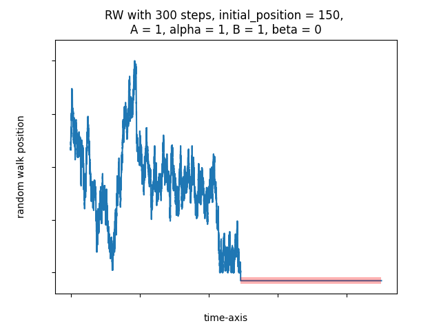
Figure 6. Elastic Brownian Motion. Here we took alpha = 1 and beta = 0. Under this choice of parameters, the random walk approximates the elastic BM, which is a mixture of being reflected and killed. Note that the cemetery state is highlighted in red in the picture above (which was automatically done in the provided Python code). Moreover, the reader can observe that, right before to the absorption time at $\Delta$, the walk touched zero many times and then jumped to the cemetery.

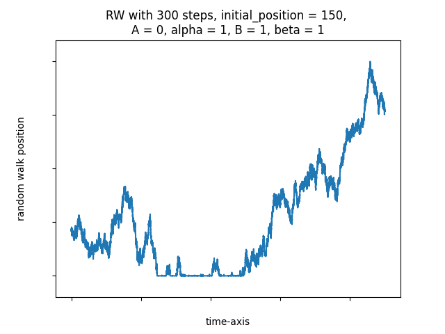
Figure 7. Sticky Brownian Motion. Here we took beta = 1 and A = 0. Under this choice of parameters, the random walk approximates the sticky Brownian motion. As we can see above, once the walk touches zero, it takes a certain time to scape from the stickiness of the origin.

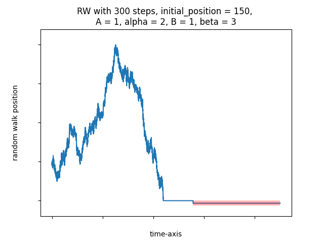
Figure 8. Exponential Holding Brownian Motion. Here we took alpha = 2 and beta = 3. Under this choice of parameters, the random walk approximates the exponential holding Brownian motion, where the walk after reaching zero, stays there for an exponential time and then jumps to the cemetery. Note that the cemetery state is highlighted in red in the picture above.

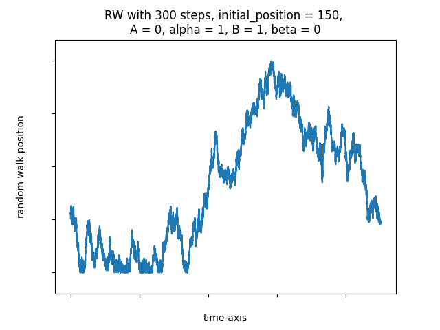
Figure 9. Reflected Brownian Motion. Here we took beta = A = 0. Under this choice of parameters, the random walk approximates the reflected Brownian motion. Note that the absence of stickiness (compare it with Figure 7).

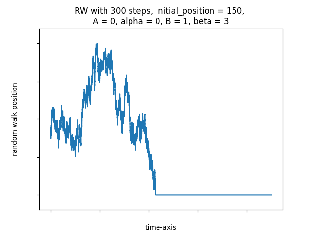
Figure 10. Absorbed Brownian motion. Here we took A = 0 and beta = 3. Under this choice of parameters, the random walk approximates the absorbed Brownian motion. Note that once the walk reaches the origin, it stays there forever.

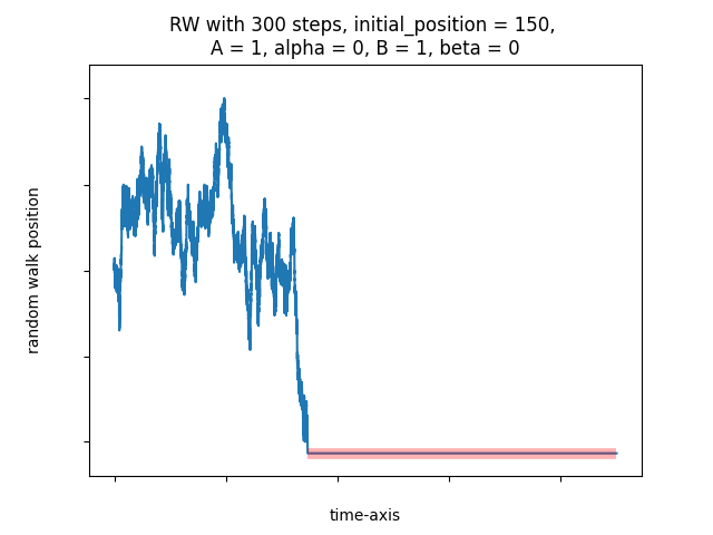
Figure 11. Killed Brownian Motion. Here we took alpha = beta = 0 and A = B = 1. Under this choice of parameters, the random walk approximates the killed BM, where the process, once reaching zero, immediately jumps to the cemetery state, which is highlighted in red.

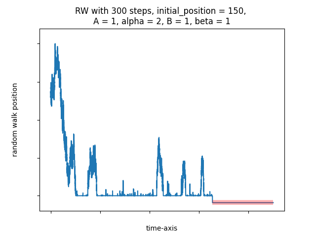
Figure 12. Mixed Brownian Motion. Here we took alpha = 2 and beta = 1. Under this choice of parameters, the random walk approximates the mixed Brownian motion. Note that the process has some stickiness at zero, and a certain random time jumps to the cemetery state, which is highlighted in red.

References

- [1] M. Amir. Sticky Brownian motion as the strong limit of a sequence of random walks. Stochastic Process. Appl., 39(2):221–237, 1991.
- [2] A. N. Borodin. Brownian local time. Uspekhi Mat. Nauk, 44(2(266)):7–48, 1989.
- [3] A. N. Borodin and P. Salminen. Handbook of Brownian motion–facts and formulae. Probab. Appl. Birkhäuser Verlag, Basel, 2002.
- [4] K. L. Chung and Z. Zhao. From Brownian Motion to Schrödinger’s Equation, pages XII, 292. Springer Berlin Heidelberg, Berlin, Heidelberg, 1995.
- [5] D. Erhard, T. Franco, and D. S. da Silva. The slow bond random walk and the snapping out Brownian motion. Ann. Appl. Probab., 31(1):99–127, 2021.
- [6] S. N. Ethier and T. G. Kurtz. Markov Processes. Wiley Series in Probability and Mathematical Statistics: Probability and Mathematical Statistics. John Wiley & Sons, Inc., New York, 1986. Characterization and convergence.
- [7] T. Franco. Boundary random walk. https://github.com/francotertu/Boundary_Random_Walk, 2024.
- [8] J. M. Harrison and A. J. Lemoine. Sticky Brownian motion as the limit of storage processes. J. Appl. Probab., 18(1):216–226, 1981.
- [9] F. B. Knight. Essentials of Brownian motion and diffusion, volume 18 of Mathematical Surveys. American Mathematical Society, Providence, R.I., 1981.
- [10] E. Kosygina, T. Mountford, and J. Peterson. Convergence of random walks with Markovian cookie stacks to Brownian motion perturbed at extrema. Probab. Theory Related Fields, 182(1-2):189–275, 2022.
- [11] A. Lejay. The snapping out Brownian motion. Ann. Appl. Probab., 26(3):1727–1742, 2016.
- [12] J. Warren. On the joining of sticky Brownian motion. In Séminaire de Probabilités, XXXIII, volume 1709 of Lecture Notes in Math., pages 257–266. Springer, Berlin, 1999.