Enhancing Multiview Synergy: Robust Learning by Exploiting the Wave Loss Function with Consensus and Complementarity Principles

Abstract

Multiview learning (MvL) is an advancing domain in machine learning, leveraging multiple data perspectives to enhance model performance through view-consistency and view-discrepancy. Despite numerous successful multiview-based support vector machine (SVM) models, existing frameworks predominantly focus on the consensus principle, often overlooking the complementarity principle. Furthermore, they exhibit limited robustness against noisy, error-prone, and view-inconsistent samples, prevalent in multiview datasets. To tackle the aforementioned limitations, this paper introduces Wave-MvSVM, a novel multiview support vector machine framework leveraging the wave loss (W-loss) function, specifically designed to harness both consensus and complementarity principles. Unlike traditional approaches that often overlook the complementary information among different views, the proposed Wave-MvSVM ensures a more comprehensive and resilient learning process by integrating both principles effectively. The W-loss function, characterized by its smoothness, asymmetry, and bounded nature, is particularly effective in mitigating the adverse effects of noisy and outlier data, thereby enhancing model stability. Theoretically, the W-loss function also exhibits a crucial classification-calibrated property, further boosting its effectiveness. The proposed Wave-MvSVM employs a between-view co-regularization term to enforce view consistency and utilizes an adaptive combination weight strategy to maximize the discriminative power of each view, thus fully exploiting both consensus and complementarity principles. The optimization problem is efficiently solved using a combination of gradient descent (GD) and the alternating direction method of multipliers (ADMM), ensuring reliable convergence to optimal solutions. Theoretical analyses, grounded in Rademacher complexity, validate the generalization capabilities of the proposed Wave-MvSVM model. Extensive empirical evaluations across diverse datasets demonstrate the superior performance of Wave-MvSVM in comparison to existing benchmark models, highlighting its potential as a robust and efficient solution for MvL challenges.

[inst1]organization=Department of Mathematics,addressline=Indian Institute of Technology Indore, city=Simrol, Indore, postcode=453552, country=India

1 Introduction

The proliferation of data across various domains has underscored the critical need for advanced methodologies that can effectively handle and integrate multiple sources of information. Multiview learning (MvL), a paradigm that seeks to leverage the complementary information available from different views or data modalities, has emerged as a potent approach to enhance learning performance [34, 33]. This approach is particularly relevant in fields such as computer vision [40, 20], bioinformatics [12, 25], and natural language processing [24, 19], where data often comes from diverse and heterogeneous sources. Conventional single-view learning techniques frequently fail to capture the intricate relationships and interactions inherent in multiview data, thereby limiting their effectiveness [44]. Consequently, there has been a significant push in the research community towards developing MvL frameworks that can seamlessly integrate and exploit the synergies among multiple views, enhancing overall learning performance.

MvL approaches can be broadly categorized into two principles: consensus and complementarity [47, 45]. The consensus principle aims to maximize the agreement among different views, ensuring that each view contributes to a unified learning objective. On the other hand, the complementarity principle emphasizes leveraging the unique information present in each view to enrich the overall model representation. Adhering to these two principles, existing MvL studies integrate multiview representations using three primary schemes: early fusion, late fusion, and a combination of both fusion types. In early fusion techniques, all views are amalgamated into a single large feature vector prior to any further processing [42, 46]. The model is then trained on this concatenated view. However, this approach often disregards the correlations and interactions among views, potentially leading to overfitting and dimensionality issues [18]. Late fusion techniques operate at the decision level by training on each view separately and subsequently combining the predictions in an ensemble manner [13, 43]. While this method offers some flexibility, it fails to fully exploit the consensus and complementary information inherent in different views. The combined fusion strategy aims to balance view-consistency and view diversity, ultimately generating the final predictors collectively. Given that views inherently describe the same objects in different feature spaces, this hybrid approach often results in superior performance across most multiview classification methods by leveraging both view-specific and shared information effectively [21, 35, 39].

Support vector machines (SVMs) [5, 22] have been a cornerstone in the realm of machine learning due to their robustness and efficacy in interpretability. SVMs are formulated within a cohesive framework that integrates regularization terms with loss functions [1, 23]. However, classical SVMs are typically designed for single-view scenarios, thereby underutilizing the multifaceted nature of data [16]. In single-view settings, SVMs optimize a hyperplane that maximizes the margin between different classes based on a single set of features [17]. This limitation has prompted researchers to explore the fusion of multiview data into the SVM framework, leading to the development of numerous multiview SVM models.

For instance, SVM-2K [10] integrates kernel canonical correlation analysis (KCCA) [48] with SVM into a single optimization framework, enforcing view-consistency constraints. Multiview Laplacian SVMs [26] extend traditional SVMs by incorporating manifold and multiview regularization, thus bridging supervised and semi-supervised learning. Additionally, Sun and Shawe-Taylor [27] introduced a general multiview framework by fusing a $\varepsilon$-insensitive loss for sparse semi-supervised learning. The multiview L2-SVM [16] capitalizes on both coherence and disparity across views by enforcing consensus among multiple views. Another significant contribution is the multiview nonparallel SVM [30], which embeds the nonparallel SVM into a multiview classification framework under the consensus constraint. Furthermore, Sun et al. [28] developed a multiview generalized eigenvalue proximal SVM by incorporating a multiview co-regularization term to maximize consensus across diverse views. In the realm of sentiment analysis, Ye et al. [41] devised a novel multiview ensemble learning method that fuses information from different features to enhance microblog sentiment classification. The aforementioned models typically adhere to either the consensus or complementarity principle, but rarely both in unison.

In recent years, numerous SVM-based MvL methodologies have proficiently integrated both the principles of consensus and complementarity. Noteworthy instances encompass multiview privileged SVM [29], multiview SVM [38] that amalgamate consensus and complementary information, and multiview twin SVM [38] with similar integration paradigms. These models predominantly utilize conventional loss functions, such as hinge loss, which inadequately capture the intricate relationships among diverse views, leading to suboptimal performance, particularly in the presence of noisy or extraneous features. To surmount these challenges, frameworks incorporating the linear-exponential (LINEX) loss function [31] and the quadratic type squared error (QTSE) loss function [14] have been introduced. Among the aforementioned models, it is notable that [31] and [14] are capable of not only fully leveraging both consistency and complementarity information but also employing asymmetric LINEX loss and QTSE loss functions, respectively. These functions adeptly differentiate between samples prone to errors and those less likely to errors, positioned between and outside the central hyperplanes. Nonetheless, these models often exhibit instability when confronted with outliers. The unbounded nature of both LINEX and QTSE loss functions permits outlier entries with substantial errors to exert disproportionate influence on the final predictor, thereby significantly skewing the decision hyperplane from its optimal position. Consequently, the implementation of a more flexible and bounded loss function is imperative to mitigate these issues and advance the field of MvL.

To advance the field of MvL, we propose the fusion of the wave loss (W-loss) function into the multiview SVM framework, seamlessly amalgamating both consensus and complementarity principles for enhanced performance and robustness. Recently, Akhtar et al. [2] developed the W-loss, which offers several advantages over traditional loss functions. It possesses nice mathematical properties, including smoothness, asymmetry, and boundedness. The smoothness characteristic of the W-loss function facilitates the use of gradient-based optimization techniques by ensuring the existence of well-defined gradients, thereby enabling efficient and reliable optimization methods. The asymmetry characteristic allows for the assignment of diverse punishments to samples depending on their propensity for misclassification. Lastly, the boundedness of the W-loss imposes an upper limit on loss values, preventing excessive influence from outliers. This upper bound is particularly advantageous in the presence of outliers, as it prevents the loss from escalating uncontrollably due to extreme errors. Theoretically, the W-loss function also exhibits a crucial classification-calibrated property. Consequently, the model becomes robust to outliers, maintaining stability and performance even in the presence of anomalous data points. Further, to enhance view-consistency, we introduce a between-view co-regularization term in the objective function, applied to the predictors of two views. Additionally, we exploit complementarity information by adaptively adjusting the combination weight for each view, which emphasizes more important and discriminative views. Thus, by fusing the W-loss function into the multiview SVM framework while adhering to both consensus and complementarity principles, we propose a novel and robust multiview SVM framework named Wave-MvSVM. The optimization problem of Wave-MvSVM is addressed using the gradient descent (GD) algorithm in conjunction with the alternating direction method of multipliers (ADMM). Additionally, the generalization capability of Wave-MvSVM is rigorously analyzed through the lens of Rademacher complexity. The main highlights of this study are encapsulated as follows:

1. We propose Wave-MvSVM, a novel multiview SVM framework that effectively amalgamates the wave loss (W-loss) function, adeptly exploiting both consensus and complementarity principles to significantly enhance performance and robustness in MvL.

2. We utilized the W-loss function as the error metric, which not only flexibly differentiates error-prone samples across both classes but also fortifies the model’s robustness against noisy and anomalous data points, maintaining stability even in challenging conditions.

3. We employed a hybrid approach combining gradient descent (GD) and the alternating direction method of multipliers (ADMM) to solve the optimization problem for Wave-MvSVM, ensuring efficient and reliable convergence to optimal solutions.

4. We rigorously analyzed the generalization capability of the proposed Wave-MvSVM framework using Rademacher complexity, thereby offering theoretical assurances for its performance across various scenarios.

5. We conducted extensive numerical experiments to validate the effectiveness of the Wave-MvSVM framework, demonstrating its superior performance in comparison to benchmark models across diverse datasets.

The remainder of this paper is organized as follows. Section 2 provides an overview of related work. Section 3 details the W-loss function and provides the mathematical formulation of the proposed Wave-MvSVM model. Section 4 presents the optimization techniques employed. Section 5 discusses the theoretical analysis of the proposed Wave-MvSVM model. Section 6 discusses the experimental setup and results, providing a thorough comparison of the proposed Wave-MvSVM with baseline models. Finally, the conclusions and potential future research directions are given in Section 7.

2 Related Work

This section begins with establishing notations and then reviews the mathematical formulation along with the solution of the SVM-2K.

2.1 Notations

Consider the sample space denoted as $\mathscr{T}$, which is a product of two distinct feature views, $1$ and $2$, expressed as $\mathscr{T}=\mathscr{T}^{[1]}\times\mathscr{T}^{[2]}$, where $\mathscr{T}^{[1]}\subseteq\mathbb{R}^{m_{1}}$, $\mathscr{T}^{[2]}\subseteq\mathbb{R}^{m_{2}}$ and $\mathscr{Y}=\{-1,+1\}$ denotes the label space. Here $m_{1}$ and $m_{2}$ denote the number of features corresponding to view $1$ and view $2$, respectively. Suppose $\mathscr{H}=\{(x_{i}^{[1]},x_{i}^{[2]},y_{i})|x_{i}^{[1]}\in\mathscr{T}^{[1]},x_{i}^{[2]}\in\mathscr{T}^{[2]},y_{i}\in\mathscr{Y}\}_{i=1}^{n}$ represent a two-view data set, where $n$ represents the number of samples.

2.2 Two view learning: SVM-2K, Theory and Practice (SVM-2K)

SVM-2K [10] finds two distinct optimal hyperplanes: one associated with view $1$ and another with view $2$, and given as:

$$w^{{[1]}^{T}}\phi_{1}(x^{[1]})+b^{[1]}=0,\hskip 11.38092pt\text{and}\hskip 11.38092ptw^{{[2]}^{T}}\phi_{2}(x^{[2]})+b^{[2]}=0.$$ (1)

The optimization problem of SVM-2K can be written as follows:

$$\underset{w_{1},w_{2},b_{1},b_{2}}{\min}\hskip 2.84544pt\leavevmode\nobreak\ \frac{1}{2}\|w_{1}\|^{2}+\frac{1}{2}\|w_{2}\|^{2}+C_{1}\sum_{i=1}^{n}\zeta_{i}^{[1]}+C_{2}\sum_{i=1}^{n}\zeta_{i}^{[2]}+D\sum_{i=1}^{n}\eta_{i}$$

s.t. $$\lvert<w_{2},\phi(x_{i}^{[2]})>+b_{2}-<w_{1},\phi(x_{i}^{[1]})>-b_{1}\rvert\leq\epsilon+\eta_{i},$$

$$y_{i}(<w^{[2]},\phi(x_{i}^{[2]})>+b^{[2]})\geq 1-\zeta_{i}^{[2]},$$

$$y_{i}(<w^{[1]},\phi(x_{i}^{[1]})>+b^{[1]})\geq 1-\zeta_{i}^{[1]},$$

$$\zeta_{i}^{[1]}\geq 0,\zeta_{i}^{[2]}\geq 0,\eta_{i}\geq 0,\leavevmode\nobreak\ \leavevmode\nobreak\ i=1,2,\ldots n,$$ (2)

where $C_{1}$, $C_{2}$, $D$ $(>0)$ are penalty parameters, $\epsilon>0$ is an insensitive parameter, $\zeta_{i}^{[1]}$, $\zeta_{i}^{[2]}$, $\eta_{i}$ are slack variables, and $\phi$ denotes the feature mapping function. The amalgamation of the two views through the $\epsilon$-insensitive $l_{1}$-norm similarity constraint is incorporated as the initial constraint in the problem (2.2).

The dual problem of (2.2) is given by:

$$\underset{q^{[1]},q^{[2]},\alpha_{i}^{[1]},\alpha_{i}^{[2]}}{\max}\hskip 1.42271pt\leavevmode\nobreak\ -\frac{1}{2}\sum_{i,j=1}^{n}(q_{i}^{[1]}q_{j}^{[1]}k_{1}(x_{i},x_{j})+q_{i}^{[2]}q_{j}^{[2]}k_{2}(x_{i},x_{j}))+\sum_{i=1}^{n}(\alpha_{i}^{[1]}+\alpha_{i}^{[2]})$$

s.t. $$q_{i}^{[1]}=\alpha_{i}^{[1]}y_{i}-\beta_{i}^{+}+\beta_{i}^{-},$$

$$q_{i}^{[2]}=\alpha_{i}^{[2]}y_{i}+\beta_{i}^{+}-\beta_{i}^{-},$$

$$\sum_{i=1}^{n}q_{i}^{[1]}=\sum_{i=1}^{n}q_{i}^{[2]}=0,$$

$$0\leq\beta_{i}^{+},\beta_{i}^{-},\beta_{i}^{+}+\beta_{i}^{-}\leq D,$$

$$0\leq\alpha_{i}^{{[1]}/{[2]}}\leq C_{1/2},$$ (3)

where $\alpha_{i}^{[1]},\alpha_{i}^{[2]},\beta_{i}^{+},\beta_{i}^{-}$ are the vectors of Lagrangian multipliers, $k_{1}(x_{i},x_{j})=<\phi(x_{i}^{[1]}),\phi(x_{j}^{[1]})>$ and $k_{2}(x_{i},x_{j})=<\phi(x_{i}^{[2]}),\phi(x_{j}^{[2]})>$ are the kernel function corresponding to view 1 and view 2, respectively. The predictive function for each view is expressed as:

$$f_{{[1]}/{[2]}}=\sum_{i=1}^{n}q_{i}^{{[1]}/{[2]}}k_{1/2}(x_{i},x)+b_{1/2}.$$ (4)

3 Proposed Work

In this section, we integrate the wave loss (W-loss) function into the multiview support vector machine framework, proposing a novel approach called the multiview support vector machine with wave loss (Wave-MvSVM). We delineate the formulation and analysis of Wave-MvSVM to elucidate how it handles multi-view representation and noisy samples concurrently. By incorporating consensus and complementarity regularization terms, Wave-MvSVM effectively learns multi-view representations. To address noisy samples, Wave-MvSVM utilizes the asymmetry of the W-loss function to adaptively apply instance-level penalties to misclassified samples. Furthermore, it leverages the bounded nature of the wave loss function to prevent the model from excessively focusing on outliers.

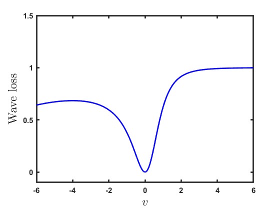
(a)

(b)

(c)

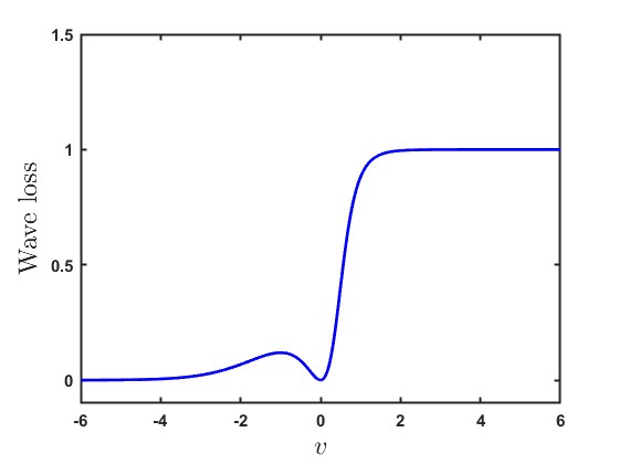
(d)

Figure 1: An illustration of the W-loss function, where $\lambda$ is fixed at $1$, and different values of $a$.

3.1 Wave loss function

In this subsection, we present the formulation of the W-loss function [2], engineered to be resilient to outliers, robust against noise, and smooth in its properties, which can be formulated as:

$$\mathcal{L}_{wave}(h)=\frac{1}{\lambda}\left(1-\frac{1}{1+\lambda h^{2}\exp{(ah)}}\right),\hskip 5.69046pt\forall\hskip 2.84544pth\in\mathbb{R},$$ (5)

where $\lambda\in\mathbb{R}^{+}$ represents the bounding parameter and $a\in\mathbb{R}$ denotes the shape parameter. Figure 1 visually illustrates the W-loss function. The W-loss function exhibits the following properties:

1. It is bounded, smooth, and asymmetric function.

2. The W-loss function possesses two essential parameters: the shape parameter $a$, dictating the shape of the loss function, and the bounding parameter $\lambda$, determining the loss function threshold values.

3. The W-loss function is differentiable and hence continuous for all $h\in\mathbb{R}$.

4. The W-loss function showcases resilience against outliers and noise insensitivity. With loss bounded to $\frac{1}{\lambda}$, it handles outliers robustly, while assigning loss to samples with $h\leq 0$, displaying resilience to noise.

5. As $a$ tends to infinity, for a fixed $\lambda$, the W-loss function converges point-wise to the $0-\frac{1}{\lambda}$ loss, expressed as:

   $$\mathcal{L}_{0-1}(h)=\left\{\begin{array}[]{lr}0&h\leq 0,\\ \frac{1}{\lambda}&h>0.\end{array}\right.$$ (8)

   Furthermore, the W-loss converges to the “$0-1$” loss when $\lambda=1$.

Figure 2: Flowchart of the model construction of Wave-MvSVM

3.2 Multiview support vector machine with W-loss (Wave-MvSVM)

In this subsubsection, we present the multiview support vector machine with wave loss (Wave-MvSVM) that utilizes the consensus and complementarity principle. The flow diagram of the model construction is shown in Figure 2. The optimization problem of Wave-MvSVM is given as follows:

$$\underset{u_{1},u_{2},\zeta^{[1]},\zeta^{[2]}}{\min} \frac{\gamma}{2}\|u_{1}\|^{2}+\frac{1}{2}\|u_{2}\|^{2}+\sum_{v=1}^{2}\sum_{i=1}^{n}\mathcal{C}_{v}\left(\frac{1}{\lambda_{v}}\left(1-\frac{1}{1+\lambda_{v}\zeta^{[v]^{2}}_{i}\exp{(a_{v}\zeta^{[v]}_{i}y_{i}})}\right)\right)$$

$$+\mathcal{D}\sum_{i=1}^{n}\left((u_{1}\phi_{1}(x^{[1]}_{i}))-(u_{2}\phi_{2}(x^{[2]}_{i}))\right)^{2}$$

s.t. $$y_{i}(u_{1}\phi_{1}(x^{[1]}_{i}))\geq 1-\zeta^{[1]}_{i},$$

$$y_{i}(u_{2}\phi_{2}(x^{[2]}_{i}))\geq 1-\zeta^{[2]}_{i},$$

$$\zeta^{[1]}_{i}\geq 0,\hskip 2.84544pt\zeta^{[2]}_{i}\geq 0,\hskip 5.69046pti=1,2,\ldots,n,$$ (9)

where $\gamma,\mathcal{C}_{1},\mathcal{C}_{2},\mathcal{D},a_{1},a_{2},\lambda_{1},\lambda_{2}>0$ are tunable parameters, $u_{1}$ and $u_{2}$ represent the weight vectors for view $1$ and view $2$, $\phi_{1}$ and $\phi_{2}$ denote the feature mapping functions, and $\zeta^{[1]}_{i}$ and $\zeta^{[2]}_{i}$ are slack variables of view $1$ and view $2$ respectively.

Each component of the optimization problem of Wave-MvSVM has the following significance:

1. The terms $u_{1}$ and $u_{2}$ serve as regularization components for views 1 and 2, respectively. These terms are used to mitigate overfitting by limiting the capacities of the classifier sets for both views. The nonnegative regularization parameter $\gamma$ determines the significance of each view to the final classifier, thus facilitating the exploration of complementary properties across different views.

2. To encourage view agreement, we incorporate a regularization term between views in the objective function $\mathcal{D}\sum_{i=1}^{n}\left((u_{1}\phi_{1}(x^{[1]}_{i}))-(u_{2}\phi_{2}(x^{[2]}_{i}))\right)^{2}$. A smaller regularization term between views tends to produce more consistent learners from both perspectives.

3. $\zeta_{i}^{[v]}$ represents a slack variable of the $v^{th}$ view, allowing Wave-MvSVM to accommodate misclassification. The W-loss function $\frac{e^{T}}{\lambda_{v}}\left(e-\frac{1}{e+\lambda_{v}\zeta^{[v]^{2}}_{i}\exp{(a_{v}\zeta^{[v]}_{i}y_{i}})}\right)$ is tailored to manage contaminated datasets with error-prone, noisy, and view-inconsistent samples. To elaborate, noisy samples are located in regions occupied by other classes, causing disturbances when determining the decision hyperplane.

Figure 3: Geometrical depiction of Wave-MvSVM: This figure demonstrates how the model handles misclassified samples, the influence of slack variables, and the application of penalties for outliers and noisy data. It provides a visual understanding of the asymmetric and bounded nature of the W-loss function, showing its impact on the decision boundary and the overall robustness of the proposed model.

Wave-MvSVM addresses noisy samples by leveraging the asymmetric and bounded nature of the W-loss function. The asymmetry allows the model to selectively impose penalties on misclassified samples at the instance level, while the boundedness ensures that noisy data does not overly influence the model’s decisions. The slack variables $\zeta^{[1]}_{i}$ and $\zeta^{[2]}_{i}$ are integrated into the W-loss function, enabling it to assess and determine the misclassification costs for different samples dynamically. The cost of misclassification for the $i^{th}$ sample in view $1$ can be denoted as $loss^{[1]}=\frac{e^{T}}{\lambda_{1}}\left(e-\frac{1}{e+\lambda_{1}\zeta^{[1]^{2}}_{i}\exp{(a_{1}\zeta^{[1]}_{i}y_{i}})}\right)$. To elucidate the mechanism of the W-loss function, we illustrate using the linear Wave-MvSVM model as depicted in Figure 3. It is worth mentioning that a comparable mechanism is also applicable to models with multiple views. In Figure 3, it is evident that for the $i^{th}$ sample, where $(x^{[1]}_{i},+1)$ is misclassified to some extent, its corresponding slack variable $\zeta^{[1]}_{i}>0$. In this scenario, we have $y_{i}\zeta^{[1]}_{i}=1\times\zeta^{[1]}_{i}>0$, resulting in a $loss^{[1]}_{i}=\frac{e^{T}}{\lambda_{1}}\left(e-\frac{1}{e+\lambda_{1}\zeta^{[1]^{2}}_{i}\exp{(a_{1}\times 1\times\zeta^{[1]}_{i}})}\right)$. Conversely, for the $j^{th}$ sample $(x^{[1]}_{j},-1)$ exhibits a certain degree of misclassification, its corresponding slack variable $\zeta^{[1]}_{j}$ is greater than zero. Consequently, we have $y_{j}\zeta^{[1]}_{j}=-1\times\zeta^{[1]}_{j}<0$, resulting in $loss^{[1]}_{j}=\frac{e^{T}}{\lambda_{1}}\left(e-\frac{1}{e+\lambda_{1}\zeta^{[1]^{2}}_{i}\exp{(a_{1}\times(-1)\times\zeta^{[1]}_{i}})}\right)$. When $a_{1}=0.5$, the shape of the W-loss function (as shown in Figure 3) indicates that $loss^{[1]}$ rises gradually with $\zeta^{[1]}$ and then decreases gradually after reaching a threshold. Moreover, the W-loss function shows a gradual decline in misclassification as the degree of error exceeds a specific threshold. Beyond this threshold, when a positive class sample is severely misclassified, deviating significantly from the hyperplane, the model may perceive it as a noisy data point and assign a lighter penalty compared to a typical sample. This property enhances the model’s resilience to outliers and noisy data. It is important to highlight that Wave-MvSVM focuses on minimizing loss for noisy samples within the positive class, which is more susceptible to containing noisy points due to its larger sample size. Furthermore, enforcing boundedness on the loss for the minority class poses a significant risk of losing valuable information, particularly considering its inherently limited representation. In summary, the W-loss function strikes a balance by appropriately penalizing misclassifications while avoiding excessive penalties for extreme misclassifications.

4 Optimizaiton for Wave-MvSVM

In this section, we use the ADMM and GD algorithms to optimize problem (3.2). Initially, we rewrite problem (3.2) using the Representer Theorem [8]. Following this, we apply the ADMM and GD algorithms to solve the optimization problem (3.2).

According to the Representer Theorem, the solutions for $u_{1}$ and $u_{2}$ in equation (3.2) can be expressed as follows:

$$u_{v}=\sum_{j=1}^{n}\alpha^{[v]}_{j}\phi_{v}(x^{[v]}_{j}),$$ (10)

where $\alpha^{[v]}=(\alpha^{[v]}_{1},\ldots,\alpha^{[v]}_{n})^{T}$ , $v=\{1,2\}$, is the coefficient vector of view $1$ and view $2$.

Substituting (10) into (3.2), we obtain:

$$\underset{u_{1},u_{2},\zeta^{[1]},\zeta^{[2]}}{\min} \frac{\gamma}{2}\alpha^{[1]^{T}}\mathcal{K}_{1}\alpha^{[1]}+\frac{1}{2}\alpha^{[2]^{T}}\mathcal{K}_{2}\alpha^{[2]}+\mathcal{C}_{1}\left(\frac{e^{T}}{\lambda_{1}}\left(e-\frac{1}{e+\lambda_{1}\zeta^{[1]^{2}}_{i}\exp{(a_{1}\zeta^{[1]}_{i}y_{i}})}\right)\right)$$

$$+\mathcal{C}_{2}\left(\frac{e^{T}}{\lambda_{2}}\left(e-\frac{1}{e+\lambda_{2}\zeta^{[2]^{2}}_{i}\exp{(a_{2}\zeta^{[2]}_{i}y_{i}})}\right)\right)+\mathcal{D}e^{T}\left(\mathcal{K}_{1}\alpha^{[1]}-\mathcal{K}_{2}\alpha^{[2]}\right)^{T}\left(\mathcal{K}_{1}\alpha^{[1]}-\mathcal{K}_{2}\alpha^{[2]}\right)$$

s.t. $$Y\mathcal{K}_{1}\alpha^{[1]}\geq 1-\zeta^{[1]},$$

$$Y\mathcal{K}_{2}\alpha^{[2]}\geq 1-\zeta^{[2]},$$

$$\zeta^{[1]}\geq 0,\hskip 2.84544pt\zeta^{[2]}\geq 0,$$ (11)

where $e$ is a vector of ones, $\mathcal{K}_{1}=k_{1}(x^{[1]}_{i},x^{[1]}_{j})=(\phi_{1}(x^{[1]}_{i}),\phi_{2}(x^{[1]}_{j}))$ and $\mathcal{K}_{2}=k_{1}(x^{[2]}_{i},x^{[2]}_{j})=(\phi_{1}(x^{[2]}_{i}),\phi_{2}(x^{[2]}_{j}))$. $\zeta^{[1]}$ and $\zeta^{[2]}$ are the slack variables, respectively. $Y=\text{diag}(y_{1},y_{2},\ldots,y_{n})$ is the $n\times n$ label matrix with $y_{1},y_{2},\ldots,y_{n}$ as its diagonal entries. To solve the problem (4), we employ the ADMM and GD algorithms to determine the optimal values of $\alpha^{[1]}$, $\alpha^{[2]}$, $\zeta^{[1]}$, and $\zeta^{[2]}$. The detailed derivation is given below.

First, by introducing slack variables $\eta_{1},\eta_{2},\eta_{3},\eta_{4}\in\mathbb{R}^{n}_{+}$, problem (4) is transformed into the following constrained problem:

$$\underset{u_{1},u_{2},\zeta^{[1]},\zeta^{[2]}}{\min} \frac{\gamma}{2}\alpha^{[1]^{T}}\mathcal{K}_{1}\alpha^{[1]}+\frac{1}{2}\alpha^{[2]^{T}}\mathcal{K}_{2}\alpha^{[2]}+\sum_{j=1}^{4}\delta_{R_{+}^{n}}(\eta_{j})+\mathcal{C}_{1}\left(\frac{e^{T}}{\lambda_{1}}\left(e-\frac{1}{e+\lambda_{1}\zeta^{[1]^{2}}_{i}\exp{(a_{1}\zeta^{[1]}_{i}y_{i}})}\right)\right)$$

$$+\mathcal{C}_{2}\left(\frac{e^{T}}{\lambda_{2}}\left(e-\frac{1}{e+\lambda_{2}\zeta^{[2]^{2}}_{i}\exp{(a_{2}\zeta^{[2]}_{i}y_{i}})}\right)\right)+\mathcal{D}e^{T}\left(\mathcal{K}_{1}\alpha^{[1]}-\mathcal{K}_{2}\alpha^{[2]}\right)^{T}\left(\mathcal{K}_{1}\alpha^{[1]}-\mathcal{K}_{2}\alpha^{[2]}\right)$$

s.t. $$Y\mathcal{K}_{1}\alpha^{[1]}-e+\zeta^{[1]}-\eta_{1}=0,$$

$$Y\mathcal{K}_{2}\alpha^{[2]}-e+\zeta^{[2]}-\eta_{2}=0,$$

$$\zeta^{[1]}-\eta_{3}=0,$$

$$\zeta^{[2]}-\eta_{4}=0,$$ (12)

where $\delta_{R_{+}^{n}}(\cdot)$ represents the indicator function on the positive real space $R_{+}^{n}$. The Lagrangian corresponding to the problem (4) is given by

$$\mathcal{L}(\alpha^{[1]},\alpha^{[2]}, \zeta^{[1]},\zeta^{[2]},\eta_{1},\eta_{2},\eta_{3},\eta_{4},\vartheta_{1},\vartheta_{2},\vartheta_{3},\vartheta_{4})=\frac{1}{2}\left(\gamma\alpha^{[1]^{T}}\mathcal{K}_{1}\alpha^{[1]}+\alpha^{[2]^{T}}\mathcal{K}_{2}\alpha^{[2]}\right)+\sum_{j=1}^{4}\delta_{R_{+}^{n}}(\eta_{j})$$

$$+\mathcal{C}_{1}\left(\frac{e^{T}}{\lambda_{1}}\left(e-\frac{1}{e+\lambda_{1}\zeta^{[1]^{2}}_{i}\exp{(a_{1}\zeta^{[1]}_{i}y_{i}})}\right)\right)+\mathcal{C}_{2}\left(\frac{e^{T}}{\lambda_{2}}\left(e-\frac{1}{e+\lambda_{2}\zeta^{[2]^{2}}_{i}\exp{(a_{2}\zeta^{[2]}_{i}y_{i}})}\right)\right)$$

$$+\mathcal{D}e^{T}\left(\mathcal{K}_{1}\alpha^{[1]}-\mathcal{K}_{2}\alpha^{[2]}\right)^{T}\left(\mathcal{K}_{1}\alpha^{[1]}-\mathcal{K}_{2}\alpha^{[2]}\right)+\vartheta_{1}^{T}\left(Y\mathcal{K}_{1}\alpha^{[1]}-e+\zeta^{[1]}-\eta_{1}\right)$$

$$+\vartheta_{2}^{T}\left(Y\mathcal{K}_{2}\alpha^{[2]}-e+\zeta^{[2]}-\eta_{2}\right)+\frac{\kappa_{1}}{2}\|Y\mathcal{K}_{1}\alpha^{[1]}-e+\zeta^{[1]}-\eta_{1}\|_{2}^{2}+\frac{\kappa_{2}}{2}\|Y\mathcal{K}_{2}\alpha^{[2]}-e+\zeta^{[2]}-\eta_{2}\|_{2}^{2}$$

$$+\vartheta_{3}^{T}(\zeta^{[1]}-\eta_{3})+\vartheta_{4}^{T}(\zeta^{[2]}-\eta_{4})+\frac{\kappa_{3}}{2}\|\zeta^{[1]}-\eta_{3}\|_{2}^{2}+\frac{\kappa_{4}}{2}\|\zeta^{[2]}-\eta_{4}\|_{2}^{2},$$ (13)

where $\vartheta_{1},\vartheta_{2},\vartheta_{3},\vartheta_{4}>0$ are the vectors of Lagrangian multipliers and $\kappa_{1},\kappa_{2},\kappa_{3},\kappa_{4}>0$ are penalty parameters.

For problem (4), ADMM is used to derive the iterative steps for obtaining its optimal solution, as detailed below:

$$\alpha^{[1]^{(t+1)}}=\underset{\alpha^{[1]}}{\arg\min}\mathcal{L}\left(\alpha^{[1]},\alpha^{[2]^{(t)}},\zeta^{[1]^{(t)}},\zeta^{[2]^{(t)}},\eta_{1}^{(t)},\eta_{2}^{(t)},\eta_{3}^{(t)},\eta_{4}^{(t)},\vartheta_{1}^{(t)},\vartheta_{2}^{(t)},\vartheta_{3}^{(t)},\vartheta_{4}^{(t)}\right),$$ (14)

$$\alpha^{[2]^{(t+1)}}=\underset{\alpha^{[2]}}{\arg\min}\mathcal{L}\left(\alpha^{[1]^{(t+1)}},\alpha^{[2]},\zeta^{[1]^{(t)}},\zeta^{[2]^{(t)}},\eta_{1}^{(t)},\eta_{2}^{(t)},\eta_{3}^{(t)},\eta_{4}^{(t)},\vartheta_{1}^{(t)},\vartheta_{2}^{(t)},\vartheta_{3}^{(t)},\vartheta_{4}^{(t)}\right),$$ (15)

$$\zeta^{[1]^{(t+1)}}=\underset{\zeta^{[1]}}{\arg\min}\mathcal{L}\left(\alpha^{[1]^{(t+1)}},\alpha^{[2]^{(t+1)}},\zeta^{[1]},\zeta^{[2]^{(t)}},\eta_{1}^{(t)},\eta_{2}^{(t)},\eta_{3}^{(t)},\eta_{4}^{(t)},\vartheta_{1}^{(t)},\vartheta_{2}^{(t)},\vartheta_{3}^{(t)},\vartheta_{4}^{(t)}\right),$$ (16)

$$\zeta^{[2]^{(t+1)}}=\underset{\zeta^{[2]}}{\arg\min}\mathcal{L}\left(\alpha^{[1]^{(t+1)}},\alpha^{[2]^{(t+1)}},\zeta^{[1]^{(t+1)}},\zeta^{[2]},\eta_{1}^{(t)},\eta_{2}^{(t)},\eta_{3}^{(t)},\eta_{4}^{(t)},\vartheta_{1}^{(t)},\vartheta_{2}^{(t)},\vartheta_{3}^{(t)},\vartheta_{4}^{(t)}\right),$$ (17)

$$\eta_{1}^{(t+1)}=\underset{\eta_{1}}{\arg\min}\mathcal{L}\left(\alpha^{[1]^{(t+1)}},\alpha^{[2]^{(t+1)}},\zeta^{[1]^{(t+1)}},\zeta^{[2]^{(t+1)}},\eta_{1},\eta_{2}^{(t)},\eta_{3}^{(t)},\eta_{4}^{(t)},\vartheta_{1}^{(t)},\vartheta_{2}^{(t)},\vartheta_{3}^{(t)},\vartheta_{4}^{(t)}\right),$$ (18)

$$\eta_{2}^{(t+1)}=\underset{\eta_{2}}{\arg\min}\mathcal{L}\left(\alpha^{[1]^{(t+1)}},\alpha^{[2]^{(t+1)}},\zeta^{[1]^{(t+1)}},\zeta^{[2]^{(t+1)}},\eta_{1}^{(t+1)},\eta_{2},\eta_{3}^{(t)},\eta_{4}^{(t)},\vartheta_{1}^{(t)},\vartheta_{2}^{(t)},\vartheta_{3}^{(t)},\vartheta_{4}^{(t)}\right),$$ (19)

$$\eta_{3}^{(t+1)}=\underset{\eta_{3}}{\arg\min}\mathcal{L}\left(\alpha^{[1]^{(t+1)}},\alpha^{[2]^{(t+1)}},\zeta^{[1]^{(t+1)}},\zeta^{[2]^{(t+1)}},\eta_{1}^{(t+1)},\eta_{2}^{(t+1)},\eta_{3},\eta_{4}^{(t)},\vartheta_{1}^{(t)},\vartheta_{2}^{(t)},\vartheta_{3}^{(t)},\vartheta_{4}^{(t)}\right),$$ (20)

$$\eta_{4}^{(t+1)}=\underset{\eta_{4}}{\arg\min}\mathcal{L}\left(\alpha^{[1]^{(t+1)}},\alpha^{[2]^{(t+1)}},\zeta^{[1]^{(t+1)}},\zeta^{[2]^{(t+1)}},\eta_{1}^{(t+1)},\eta_{2}^{(t+1)},\eta_{3}^{(t+1)},\eta_{4},\vartheta_{1}^{(t)},\vartheta_{2}^{(t)},\vartheta_{3}^{(t)},\vartheta_{4}^{(t)}\right),$$ (21)

$$\vartheta_{1}^{(t+1)}=\vartheta_{1}^{(t)}+\theta_{1}\kappa_{1}(Y\mathcal{K}_{1}\alpha^{[1]^{(t+1)}}-e+\zeta^{[1]^{(t+1)}}-\eta_{1}^{(t+1)}),$$ (22)

$$\vartheta_{2}^{(t+1)}=\vartheta_{2}^{(t)}+\theta_{2}\kappa_{2}(Y\mathcal{K}_{2}\alpha^{[2]^{(t+1)}}-e+\zeta^{[2]^{(t+1)}}-\eta_{2}^{(t+1)}),$$ (23)

$$\vartheta_{3}^{(t+1)}=\vartheta_{3}^{(t)}+\theta_{1}\kappa_{3}(\zeta^{[1]^{(t+1)}}-\eta_{3}^{(t+1)}),$$ (24)

$$\vartheta_{4}^{(t+1)}=\vartheta_{4}^{(t)}+\theta_{2}\kappa_{4}(\zeta^{[2]^{(t+1)}}-\eta_{4}^{(t+1)}),$$ (25)

where $\theta_{1},\theta_{2}\in\left(0,\frac{\sqrt{5}+1}{2}\right)$ are the dual step lengths. Using the equation provided above, we can compute the closed-form solutions for the vectors $\alpha^{[1]}$, $\alpha^{[2]}$, Lagrange multiplier vectors $\vartheta_{1},\vartheta_{2},\vartheta_{3},\vartheta_{4}$ and slack variables $\kappa_{1},\kappa_{2},\kappa_{3},\kappa_{4}$. The optimal slack variables $\zeta^{[1]}$ and $\zeta^{[2]}$ can be determined by the GD algorithm keeping $\alpha^{[1]},\alpha^{[2]},\kappa_{1},\kappa_{2},\kappa_{3},\kappa_{4},\vartheta_{1},\vartheta_{2},\vartheta_{3},\vartheta_{4}$ fixed. The objective function for the GD algorithm is given by:

$$\underset{\zeta^{[1]},\zeta^{[2]}}{\min}\mathcal{L}_{\zeta} =\mathcal{C}_{1}\left(\frac{e^{T}}{\lambda_{1}}\left(e-\frac{1}{e+\lambda_{1}\zeta^{[1]^{2}}_{i}\exp{(a_{1}\zeta^{[1]}_{i}y_{i}})}\right)\right)+\mathcal{C}_{2}\left(\frac{e^{T}}{\lambda_{2}}\left(e-\frac{1}{e+\lambda_{2}\zeta^{[2]^{2}}_{i}\exp{(a_{2}\zeta^{[2]}_{i}y_{i}})}\right)\right)$$

$$+\vartheta_{1}^{T}\left(Y\mathcal{K}_{1}\alpha^{[1]}-e+\zeta^{[1]}-\eta_{1}\right)+\vartheta_{2}^{T}\left(Y\mathcal{K}_{2}\alpha^{[2]}-e+\zeta^{[2]}-\eta_{2}\right)+\frac{\kappa_{1}}{2}\|Y\mathcal{K}_{1}\alpha^{[1]}-e+\zeta^{[1]}-\eta_{1}\|_{2}^{2}$$

$$+\frac{\kappa_{2}}{2}\|Y\mathcal{K}_{2}\alpha^{[2]}-e+\zeta^{[2]}-\eta_{2}\|_{2}^{2}+\vartheta_{3}^{T}(\zeta^{[1]}-\eta_{3})+\vartheta_{4}^{T}(\zeta^{[2]}-\eta_{4})+\frac{\kappa_{3}}{2}\|\zeta^{[1]}-\eta_{3}\|_{2}^{2}+\frac{\kappa_{4}}{2}\|\zeta^{[2]}-\eta_{4}\|_{2}^{2}.$$ (26)

Based on problem (4), we can compute the gradients of $\mathcal{L}_{\zeta}$ w.r.t. $\zeta^{[1]}$ and $\zeta^{[2]}$, respectively.

$$\nabla\mathcal{L}_{\zeta^{[1]}}=\mathcal{C}_{1}\zeta^{[1]}\exp{(a_{1}Y\zeta^{[1]})}\left[\frac{2e+\zeta^{[1]}a_{1}Y}{(e+\lambda_{1}\zeta^{[1]^{2}}\exp{(a_{1}Y\zeta^{[1]})})^{2}}\right]+\vartheta_{1}+\vartheta_{3}\kappa_{1}(Y\mathcal{K}_{1}\alpha^{[1]}-e+\zeta^{[1]}-\eta_{1})+\kappa_{3}+(\zeta^{[1]}-\eta_{3}),$$ (27)

and

$$\nabla\mathcal{L}_{\zeta^{[2]}}=\mathcal{C}_{2}\zeta^{[2]}\exp{(a_{2}Y\zeta^{[2]})}\left[\frac{2e+\zeta^{[2]}a_{2}Y}{(e+\lambda_{2}\zeta^{[2]^{2}}\exp{(a_{2}Y\zeta^{[2]})})^{2}}\right]+\vartheta_{2}+\vartheta_{4}+\kappa_{2}(Y\mathcal{K}_{2}\alpha^{[2]}-e+\zeta^{[2]}-\eta_{2})+\kappa_{4}(\zeta^{[2]}-\eta_{4}).$$ (28)

The GD algorithm for solving $\zeta^{[1]}$ and $\zeta^{[2]}$ is outlined in the Algorithm 1. Building on this, we outline the detailed iterative steps for the ADMM algorithm in the Algorithm 2.

Algorithm 1 GD algorithm for Wave-MvSVM

Input: Input dataset $\{(x_{i}^{[1]},x_{i}^{[2]},y_{i})\}_{i=1}^{n}$, $y_{i}\in\{-1,1\}$, W-loss parameters $a_{1}$, and $a_{2}$, penalty parameters $\mathcal{C}_{1}$, and $\mathcal{C}_{2}$, ADMM parameters $\kappa_{1},\kappa_{2},\kappa_{3}$, and $\kappa_{4}$ and maximum iteration number $Iter$.
Output: Optimal values $\zeta^{[1]^{*}}$ and $\zeta^{[2]^{*}}$

1:  Initialize: $\zeta^{[1]^{(0)}}$, $\zeta^{[2]^{(0)}}$;

2:  while not converge do

3:  $\zeta^{[1]^{(t+1)}}=\zeta^{[1]^{(t)}}-\delta\nabla\mathcal{L}_{\zeta^{[1]}}$;

4:  $\zeta^{[2]^{(t+1)}}=\zeta^{[2]^{(t)}}-\delta\nabla\mathcal{L}_{\zeta^{[2]}}$;

5:  end while

6:  Return: $\zeta^{[1]^{*}}$ and $\zeta^{[2]^{*}}$.

Algorithm 2 ADMM algorithm for Wave-MvSVM

Input: Input dataset $\{(x_{i}^{[1]},x_{i}^{[2]},y_{i})\}_{i=1}^{n}$, $y_{i}\in\{-1,1\}$, W-loss parameters $a_{1},a_{2}$, penalty parameters $\mathcal{C}_{1},\mathcal{C}_{2}$, ADMM parameters $\kappa_{1},\kappa_{2},\kappa_{3},\kappa_{4}$ and maximum iteration number $Iter$.
Output: Model parameters

1:  Initialize: $\alpha^{[1]^{(0)}},\alpha^{[2]^{(0)}},\zeta^{[1]^{(0)}},\zeta^{[2]^{(0)}},\eta_{1}^{(0)},\eta_{2}^{(0)},\eta_{3}^{(0)},\eta_{4}^{(0)}$, $\vartheta_{1}^{(0)},\vartheta_{2}^{(0)},\vartheta_{3}^{(0)},\vartheta_{4}^{(0)}$.

2:  while not converge do

3:  $\alpha^{[1]^{(t+1)}}=(\gamma_{1}\mathcal{K}_{1}+2\mathcal{D}\mathcal{K}_{1}^{T}\mathcal{K}_{1}+\kappa_{1}\mathcal{K}_{1}^{T}\mathcal{K}_{1})^{-1}$ $(2\mathcal{D}\mathcal{K}_{1}^{T}\mathcal{K}_{2}\alpha^{[2]^{(t)}}-Y\mathcal{K}_{1}\vartheta_{1}^{(t)}+\kappa_{1}Y\mathcal{K}_{1}(e-\zeta^{[1]^{(t)}}+\eta_{1}^{[t]}))$;

4:  $\alpha^{[2]^{(t+1)}}=(\gamma_{2}\mathcal{K}_{2}+2\mathcal{D}\mathcal{K}_{2}^{T}\mathcal{K}_{2}+\kappa_{2}\mathcal{K}_{2}^{T}\mathcal{K}_{2})^{-1}$ $(2\mathcal{D}\mathcal{K}_{2}^{T}\mathcal{K}_{1}\alpha^{[1]^{(t+1)}}-Y\mathcal{K}_{2}\vartheta_{2}^{(t)}+\kappa_{2}Y\mathcal{K}_{2}(e-\zeta^{[2]^{(t)}}+\eta_{2}^{[t]}))$;

5:  $\zeta^{[1]^{(t+1)}}=\textbf{GD}(\mathcal{L}(\alpha^{[1]^{(t+1)}},\alpha^{[2]^{(t+1)}},\zeta^{[1]},\zeta^{[2]^{(t)}},\eta_{1}^{(t)},\eta_{2}^{(t)},\eta_{3}^{(t)},\eta_{4}^{(t)},\vartheta_{1}^{(t)},\vartheta_{2}^{(t)},\vartheta_{3}^{(t)},\vartheta_{4}^{(t)})$;

6:  $\zeta^{[2]^{(t+1)}}=\textbf{GD}(\mathcal{L}(\alpha^{[1]^{(t+1)}},\alpha^{[2]^{(t+1)}},\zeta^{[1]^{(t+1)}},\zeta^{[2]},\eta_{1}^{(t)},\eta_{2}^{(t)},\eta_{3}^{(t)},\eta_{4}^{(t)},\vartheta_{1}^{(t)},\vartheta_{2}^{(t)},\vartheta_{3}^{(t)},\vartheta_{4}^{(t)}))$;

7:  $\eta_{1}^{(t+1)}=\prod_{R_{+}^{n}}(\vartheta_{1}^{(t)}/\kappa_{1}+(Y\mathcal{K}_{1}\alpha^{[1]^{(t+1)}}-e+\zeta^{[1]^{(t+1)}}))$;

8:  $\eta_{2}^{(t+1)}=\prod_{R_{+}^{n}}(\vartheta_{2}^{(t)}/\kappa_{2}+(Y\mathcal{K}_{1}\alpha^{[2]^{(t+1)}}-e+\zeta^{[2]^{(t+1)}}))$;

9:  $\eta_{3}^{(t+1)}=\prod_{R_{+}^{n}}(\vartheta_{3}^{(t)}/\kappa_{3}+\zeta^{[1]^{(t+1)}})$;

10:  $\eta_{4}^{(t+1)}=\prod_{R_{+}^{n}}(\vartheta_{4}^{(t)}/\kappa_{4}+\zeta^{[2]^{(t+1)}})$;

11:  $\vartheta_{1}^{(t+1)}=\vartheta_{1}^{t}+\tau_{1}\kappa_{1}(Y\mathcal{K}_{1}\alpha^{[1]^{(t+1)}}-e+\zeta^{[1]^{(t+1)}}+\eta_{1}^{(t+1)})$;

12:  $\vartheta_{2}^{(t+1)}=\vartheta_{2}^{t}+\tau_{2}\kappa_{2}(Y\mathcal{K}_{2}\alpha^{[2]^{(t+1)}}-e+\zeta^{[2]^{(t+1)}}+\eta_{2}^{(t+1)})$;

13:  $\vartheta_{3}^{(t+1)}=\vartheta_{3}^{t}+\tau_{1}\kappa_{3}(\zeta^{[1]^{(t+1)}}-\eta_{3}^{(t+1)})$;

14:  $\vartheta_{4}^{(t+1)}=\vartheta_{4}^{t}+\tau_{2}\kappa_{4}(\zeta^{[2]^{(t+1)}}-\eta_{4}^{(t+1)})$;

15:  end while

16:  Return: Optimal $\alpha^{[1]^{*}}$ and $\alpha^{[2]^{*}}$.

After obtaining the optimal values $\alpha^{[1]*}$ and $\alpha^{[2]*}$ for the optimization problem (4), the class label of a new sample $(x^{[1]},x^{[2]})$ can be determined as follows:

$$g(x^{[1]},x^{[2]})=sign(f(x^{[1]},x^{[2]})),$$ (29)

where

$$f(x^{[1]},x^{[2]})=\gamma\sum_{i=1}^{n}\alpha^{[1]^{*}}_{i}k_{1}(x^{[1]}_{i},x^{[1]})+\sum_{i=1}^{n}\alpha^{[2]^{*}}_{i}k_{2}(x^{[2]}_{i},x^{[2]}).$$ (30)

5 Theoretical Analysis

We discuss the complexity analysis of the proposed Wave-MvSVM model in subsection 5.1. We delve into the theoretical analysis of the W-loss function in subsection 5.2. To thoroughly verify the generalization performance of Wave-MvSVM, in Section 5.3, we utilize Rademacher complexity theory to theoretically examine the generalization error bound and the consistency error bound of Wave-MvSVM.

5.1 Computational complexity

In this subsection, we outline the computational complexity of Wave-MvSVM. The optimization problem for Wave-MvSVM is solved using ADMM and GD methods. Updating $\alpha^{[1]}$ and $\alpha^{[2]}$ with ADMM involves a computational complexity of $\mathcal{O}(T_{1}\times n^{3})$, where $n$ represents the number of samples and $T_{1}$ is the number of iterations. Updating $\zeta^{[1]}$ and $\zeta^{[2]}$ with GD has a computational complexity of $\mathcal{O}(T_{1}\times T_{2}\times n^{2})$, where $T_{2}$ denotes the number of iterations. The complexity for updating $\eta_{1}$, $\eta_{2}$, $\vartheta_{1}$, and $\vartheta_{2}$ using ADMM is $\mathcal{O}(T_{1}\times n^{2})$, while updating $\eta_{3}$, $\eta_{4}$, $\vartheta_{3}$, and $\vartheta_{4}$ has a complexity of $\mathcal{O}(T_{1}\times n)$. Therefore, the overall complexities for the ADMM and GD algorithms are $\mathcal{O}(T_{1}\times n^{3})+\mathcal{O}(T_{1}\times n^{2})+\mathcal{O}(T_{1}\times n)$ and $\mathcal{O}(T_{1}\times T_{2}\times n^{2})$, respectively. Consequently, the total computational complexity of Wave-MvSVM is given by $\mathcal{O}(T_{1}\times n^{3})+\mathcal{O}(T_{1}\times n^{2})+\mathcal{O}(T_{1}\times n)+\mathcal{O}(T_{1}\times T_{2}\times n^{2})\approx\mathcal{O}(T_{1}\times n^{3})+\mathcal{O}(T_{1}\times T_{2}\times n^{2})$.

5.2 W-loss function theoretical analysis

In this subsection, we explore the theoretical foundations of the W-loss function, shedding light on its crucial classification-calibrated nature [2]. Classification calibration, as introduced by Bartlett et al. [4], serves as a method for assessing the statistical effectiveness of loss functions. Classification calibration guarantees that the probabilities predicted by the model align closely with the actual likelihood of events, enhancing the reliability of the model’s predictions. This aspect is crucial in deepening our understanding of how the W-loss function performs in classification tasks.

Suppose we have a training dataset $\mathcal{X}=\{(x_{i},y_{i})\}_{i=1}^{n}$, where each sample $x_{i}$ is paired with a label $y_{i}$, and these samples are drawn independently from a probability distribution $\mathcal{P}$. The probability distribution $\mathcal{P}$ encompasses both the input space $X\subset\mathbb{R}^{n}$ and the corresponding label space $Y=\{-1,+1\}$. The main objective is to create a binary classifier $\mathcal{E}$ that can do input processing in the $X$ space and classify inputs into one of the labels in $Y$. Generating a classifier that minimizes the related error is the main goal of this classification challenge. One can express the risk associated with a given classifier $\mathcal{E}$ using the following formulation:

$$\mathcal{G}(\mathcal{E})=\int_{X}\mathcal{P}(\mathcal{E}(x)\neq y|x)d\mathcal{P}_{X}.$$ (31)

Here, the probability distribution of the label $y$ given an input $x$ is represented by $\mathcal{P}(y|x)$, and $d\mathcal{P}_{X}$ denotes the marginal distribution of the input $x$. Furthermore, the conditional distribution $\mathcal{P}(y|x)$ is binary, implying it is governed by $\mathcal{P}(x)=\text{Prob}(y=1|x)$ and $1-\mathcal{P}(x)=\text{Prob}(y=-1|x)$. In essence, the goal is to create a classifier that precisely categorizes inputs, reducing the overall classification error.

When $\mathcal{P}(x)$ is not equal to $\frac{1}{2}$, the Bayes classifier can be described as follows:

$$\mathcal{F}_{\mathcal{E}}(x)=\left\{\begin{array}[]{lr}-1&\mathcal{P}(x)<\frac{1}{2},\\ 1&\mathcal{P}(x)>\frac{1}{2}.\end{array}\right.$$ (34)

It has been shown that the Bayes classifier minimizes classification error optimally. This can be expressed mathematically as:

$$\mathcal{F}_{\mathcal{E}}=\underset{\mathcal{E}:X\rightarrow Y}{\arg\min}\mathcal{G}(\mathcal{E}).$$ (35)

For a given loss function $\mathcal{L}$, the expected error of a classifier $\mathcal{F}:X\rightarrow\mathbb{R}$ can be formulated as follows:

$$\mathcal{G}_{\mathcal{L},\mathcal{P}}(\mathcal{F})=\int_{X\times Y}\mathcal{L}(1-y\mathcal{F}(x))d\mathcal{P}.$$ (36)

$\mathcal{F}_{\mathcal{L},\mathcal{P}}$ aimed at minimizing the expected error across all feasible functions, is expressed as follows:

$$\mathcal{F}_{\mathcal{L},\mathcal{P}}(x)=\underset{\mathcal{F}(x)\in\mathbb{R}}{\arg\min}\int_{Y}\mathcal{L}(1-y\mathcal{F}(x))d\mathcal{P}(y|x),\leavevmode\nobreak\ \leavevmode\nobreak\ \forall\leavevmode\nobreak\ \leavevmode\nobreak\ x\in X.$$ (37)

The W-loss function $\mathcal{L}_{\text{wave}}(\cdot)$ satisfies Theorem 5.1, demonstrating its classification-calibrated nature [2]. This property guarantees that minimizing the expected error corresponds to the sign of the Bayes classifier, underscoring the importance of the W-loss function.

Theorem 5.1.

[2]: The W-loss function $\mathcal{L}_{\text{wave}}(v)$ is characterized by classification calibration, ensuring that $\mathcal{F}_{\mathcal{L}_{\text{wave}},\mathcal{P}}$ shares the same sign as the Bayes classifier.

Proof.

We get the following outcome from a simple calculation:

$$\int_{Y}\mathcal{L}_{wave} (1-y\mathcal{F}(x))d\mathcal{P}(y|x)=\mathcal{L}_{wave}(1+\mathcal{F}(x))(1-\mathcal{P}(x))+\mathcal{L}_{wave}(1-\mathcal{F}(x))\mathcal{P}(x)$$

$$=\frac{1}{\eta}\left(1-\frac{1}{1+\eta(1+\mathcal{F}(x))^{2}e^{\gamma(1+\mathcal{F}(x))}}\right)(1-\mathcal{P}(x))+\frac{1}{\eta}\left(1-\frac{1}{1+\eta(1-\mathcal{F}(x))^{2}e^{\gamma(1-\mathcal{F}(x))}}\right)\mathcal{P}(x).$$ (38)

The graphical depiction of $\int_{Y}\mathcal{L}_{\text{wave}}(1-y\mathcal{F}(x))d\mathcal{P}(y|x)$ as functions of $\mathcal{F}(x)$ are shown in Figures 4(a) and 4(b), respectively, for the situations where $\mathcal{P}(x)>1/2$ and $\mathcal{P}(x)<1/2$. Figure 4 demonstrates that the minimum value of $\int_{Y}\mathcal{L}_{\text{wave}}(y-\mathcal{F}(x))d\mathcal{P}(y|x)$ corresponds to a positive $\mathcal{F}(x)$ when $\mathcal{P}(x)>1/2$. In contrast, when $\mathcal{P}(x)<1/2$, the minimum value corresponds to a negative value of $\mathcal{F}(x)$.

Therefore, the trends depicted in Figures 4(a) and 4(b) confirm that the W-loss function $\mathcal{L}_{\text{wave}}(v)$ is classification-calibrated. ∎

(a)

(b)

Figure 4: Graphically represent $\int_{Y}\mathcal{L}_{\text{wave}}(1-y\mathcal{F}(x))d\mathcal{P}(y|x)$ as a function of $\mathcal{F}(x)$, considering various values of $\mathcal{P}(x)$. (a) Illustrate the case where $\mathcal{P}(x)>1/2$. (b) Depict the case when $\mathcal{P}(x)<1/2$.

5.3 Generalization capability analysis

In this subsection, we introduce the generalization error bound for Wave-MvSVM. To start, we define the Rademacher complexity [3]:

Definition 1.

Let $\mathcal{Q}$ represent the probability distribution over the set $T$, where $T=\{x_{1},\ldots,x_{n}\}$ consists of $n$ independent samples drawn from $\mathcal{Q}$. For a function set $\mathscr{G}$ defined on $T$, the empirical Rademacher complexity on $\mathscr{G}$ is defined as:

$$\hat{R}_{n}(\hat{\mathscr{G}}) =\mathbb{E}_{\sigma}\left[\underset{g\in\mathscr{G}}{\sup}|\frac{2}{n}\sum_{i=1}^{n}\sigma_{i}g(x_{i})|:x_{1},x_{2},\ldots,x_{n}\right],$$ (39)

where $\sigma=(\sigma_{1},\ldots,\sigma_{n})$ are independent Rademacher random variables taking values $\{+1,-1\}$. The Rademacher complexity of $\mathscr{G}$ is given by:

$$R_{n}(\mathscr{G}) =\hat{\mathbb{E}}_{T}[\hat{R_{n}}(\mathscr{G})]=\hat{\mathbb{E}}_{T\sigma}\left[\underset{g\in\mathscr{G}}{\sup}|\frac{2}{n}\sum_{i=1}^{n}\sigma_{i}g(x_{i})|\right].$$ (40)

Lemma 5.2.

Choose $\theta$ from the interval $(0,1)$ and consider $\mathscr{G}$ as a class of functions mapping from an input space $T$ to $[0,1]$. Suppose $\{x_{i}\}_{i=1}^{n}$ be independently drawn from a probability distribution $\mathcal{Q}$. Then, with a probability of at least $1-\theta$ over random samples of size $n$, every $g\in\mathscr{G}$ satisfies:

$$\mathbb{E}_{\mathcal{Q}}[g(x)]\leq\hat{\mathbb{E}}_{\mathcal{Q}}[g(x)]+\hat{R}_{n}(\mathscr{G})+3\sqrt{\frac{\ln(2/\theta)}{2n}}.$$ (41)

Lemma 5.3.

let $T=\{(x_{i},y_{i})\}_{i=1}^{n}$ be a sample set from $X$ and assume $\mathcal{K}:X\times X\rightarrow\mathbb{R}$ is a kernel. For the function class $\mathscr{G}_{B}=\{g|g:x\rightarrow(u\cdot\phi(x)):\|u\|\leq B\}$ in the kernel feature space, the empirical Rademacher complexity of $\mathscr{G}_{B}$ satisfies:

$$\hat{R}_{n}(\mathscr{G}_{B})=\frac{2B}{n}\sqrt{\sum_{i=1}^{n}\mathcal{K}(x_{i},x_{i})}.$$ (42)

Lemma 5.4.

Consider $\mathscr{A}$ as a Lipschitz function with a Lipschitz constant $\mathcal{L}$, mapping the real numbers to the real numbers, satisfying $\mathscr{A}(0)=0$. The Rademacher complexity of the class $\mathscr{A}\circ\mathscr{G}$ is:

$$\hat{R}_{n}(\mathscr{A}\circ\mathscr{G})\leq 2\mathcal{L}\hat{R}_{n}(\mathscr{G}).$$ (43)

As shown in equation (29), we utilize the weighted predictions from the two views as the prediction function in Wave-MvSVM. Consequently, we can derive the generalization error bound of Wave-MvSVM using the following theorem.

Theorem 5.5.

Given $N\in\mathbb{R}^{+}$, $\theta\in(0,1)$, and a training set $T=\{(x_{i},y_{i})\}_{i=1}^{n}$ drawn independently and identically from probability distribution $\mathcal{Q}$, where $y_{i}\in\{-1,+1\}$ and $x_{i}=(x_{i}^{A};\delta x_{i}^{B})$. Define the function class classes $\mathscr{G}=\{g|g:x\rightarrow u^{T}\hat{\phi}(x),\|u\|\leq N\}$ and $\hat{\mathscr{G}}=\{\hat{g}|\hat{g}:(x,y)\rightarrow yg(x),g(x)\in\mathscr{G}\}$, where $u=(u_{1};u_{2})$, $\hat{\phi}(x)=(\phi_{1}(x_{i}^{[1]});\phi_{2}(x_{i}^{[2]}))$ and $g(x)=\left(u_{1}^{T}\phi_{1}(x^{[1]})+\delta u_{2}^{T}\phi_{2}(x^{[2]})\right)=u^{T}\hat{\phi}(x)\in\mathscr{G}$. Then, with a probability of at least $1-\theta$ over $T$, every $g(x)\in\mathscr{G}$ satisfies

$$\mathbb{P}_{\mathcal{Q}}[yg(x)\leq 0]\leq\frac{1}{n(1+\delta)}\sum_{i=1}^{n}(\zeta_{i}^{[1]}+\delta\zeta_{i}^{[2]})+3\sqrt{\frac{\ln(2/\theta)}{2n}}+\frac{4N}{n(1+\delta)}\sqrt{\sum_{i=1}^{n}(\mathcal{K}_{1}(x_{i}^{[1]},x_{i}^{[1]})+\delta^{2}\mathcal{K}_{2}(x_{i}^{[2]},x_{i}^{[2]}))}.$$ (44)

Proof.

Let’s consider a loss function $\Omega:\mathbb{R}\rightarrow[0,1]$ defined as:

$$\Omega(x)=\left\{\begin{array}[]{lll}{1},&\text{if}\leavevmode\nobreak\ \leavevmode\nobreak\ x<0,\vspace{3mm}\\ {1-\frac{x}{1+\delta}},&\text{if}\leavevmode\nobreak\ \leavevmode\nobreak\ 0\leq x\leq 1+\delta,\\ {0},&otherwise.\end{array}\right.$$ (48)

Then, we have

$$\mathbb{P}_{\mathcal{Q}}[yg(x)\leq 0]\leq\mathbb{E}_{\mathcal{Q}}[\Omega(\hat{g}(x,y))].$$ (49)

Using Lemma 5.2, we have

$$\mathbb{E}_{\mathcal{Q}}[\Omega(\hat{g}(x,y))-1] \leq\hat{\mathbb{E}}_{T}[\Omega(\hat{g}(x,y))-1]+3\sqrt{\frac{\ln(2/\theta)}{2n}}+\hat{R}_{n}((\Omega-1)\circ\mathscr{G}).$$ (50)

Therefore,

$$\mathbb{E}_{\mathcal{Q}}[\Omega(\hat{g}(x,y))]\leq \hat{\mathbb{E}}_{T}[\Omega(\hat{g}(x,y))]+3\sqrt{\frac{\ln(2/\theta)}{2n}}+\hat{R}_{n}((\Omega-1)\circ\mathscr{G}).$$ (51)

From the first and second constraints in Wave-MvSVM, we deduce:

$$\hat{\mathbb{E}}_{T}[\Omega(\hat{g}(x,y))] \leq\frac{1}{n(1+\delta)}\sum_{i=1}^{n}[1+\delta-y_{i}g(x_{i})]_{+}$$

$$=\frac{1}{n(1+\delta)}\sum_{i=1}^{n}[1-y_{i}g_{1}(x_{i}^{[1]})+\delta(1-y_{i}g_{2}(x_{i}^{[2]}))]_{+}$$

$$\leq\frac{1}{n(1+\delta)}\sum_{i=1}^{n}\{[1-y_{i}g_{1}(x_{i}^{[1]})]_{+}+\delta[1-y_{i}g_{2}(x_{i}^{[2]})]_{+}\}$$

$$\leq\frac{1}{n(1+\delta)}\sum_{i=1}^{n}(\zeta_{i}^{[1]}+\delta\zeta_{i}^{[2]}).$$ (52)

Considering that $(\Omega-1)(x)$ is a Lipschitz function with a constant of $\frac{1}{1+\delta}$, which intersects the origin and is uniformly bounded, we can establish the following inequality based on Lemma 5.4:

$$\hat{R}_{n}((\Omega-1)\circ\hat{\mathscr{G}})\leq\frac{2}{1+\delta}\hat{R}_{n}(\hat{\mathscr{G}}).$$ (53)

Using the Definition 1, we obtain:

$$\hat{R}_{n}(\hat{\mathscr{G}}) =\mathbb{E}_{\sigma}\left[\underset{\hat{g}\in\hat{\mathscr{G}}}{\sup}|\frac{2}{n}\sum_{i=1}^{n}\sigma_{i}\hat{g}(x_{i},y_{i})\right]$$

$$=\mathbb{E}_{\sigma}\left[\underset{g\in\mathscr{G}}{\sup}|\frac{2}{n}\sum_{i=1}^{n}\sigma_{i}y_{i}g(x_{i})\right]$$

$$=\mathbb{E}_{\sigma}\left[\underset{g\in\mathscr{G}}{\sup}|\frac{2}{n}\sum_{i=1}^{n}\sigma_{i}g(x_{i})\right]$$

$$=\hat{R}_{n}(\mathscr{G}).$$ (54)

Combining this with Lemma 5.3, we have:

$$\hat{R}_{n}((\Omega-1)\circ\hat{\mathscr{G}}) \leq\frac{2}{1+\delta}\hat{R}_{n}(\mathscr{G})$$

$$=\frac{4N}{n(1+\delta)}\sqrt{\sum_{i=1}^{n}\hat{\mathcal{K}}(x_{i},x_{i})}$$

$$=\frac{4N}{n(1+\delta)}\sqrt{\sum_{i=1}^{n}(\mathcal{K}_{1}(x_{i}^{[1]},x_{i}^{[1]})+\delta^{2}\mathcal{K}_{2}(x_{i}^{[2]},x_{i}^{[2]}))}.$$ (55)

Moreover, by combining equations (49), (51), (5.3), and (5.3), we can obtain inequality, which demonstrates the generalization error bound of Wave-MvSVM. ∎

We define the classification error function $g(x)$ using the integrated decision function defined in Wave-MvSVM (3.2). By integrating the empirical Rademacher complexity of $\mathcal{G}$ with the empirical expectation of $\hat{\mathcal{G}}$, we establish a margin-based estimate of the misclassification probability. As $n$ increases significantly, Wave-MvSVM demonstrates a robust generalization error bound for classification tasks. As the training error decreases, the generalization error also decreases accordingly. This theoretically ensures that Wave-MvSVM achieves superior generalization performance.

6 Numerical Experiments

To assess the effectiveness of the proposed Wave-MvSVM model, we evaluate their performance against baseline models including SVM-2K [10], MvTwSVM [37], MVNPSVM [30], PSVM-2V [29], MVLDM [15] and MVCSKL [32]. We conduct experiments on publicly available benchmark datasets, which include $30$ real-world UCI [9] and KEEL [7] datasets, as well as $45$ binary classification datasets obtained from the Animal with Attributes (AwA) dataset.

6.1 Experimental setup

The experimental hardware setup consists of a PC featuring an Intel(R) Xeon(R) Gold $6226$R CPU operating at $2.90$GHz, with $128$ GB of RAM, and running the Windows $11$ operating system. The experiments are conducted using Matlab R$2023$a. The dataset is randomly partitioned into a $70:30$ ratio, allocating $70\%$ of the data for training and $30\%$ for testing. We utilize a five-fold cross-validation technique along with a grid search approach to optimize the hyperparameters of the models. For all experiments, we opt for the Gaussian kernel function represented by $\mathcal{K}(x_{i},x_{j})=e^{-\frac{\|x_{i}-x_{j}\|^{2}}{2\sigma^{2}}}$ for each model. The kernel parameter $\sigma$ is selected from the following range: $\{2^{-5},2^{-4},\ldots,2^{4},2^{5}\}$. The parameters $\mathcal{C}_{1}$, $\mathcal{C}_{2}$, and $\mathcal{D}$ are selected from $\{2^{-2},2^{-1},1,2^{1},2^{2}\}$. W-loss function parameters $\lambda_{1}$ and $\lambda_{2}$ are selected from the range $\{0.2,0.4,0.6,0.8,1\}$, and the other parameters $a_{1}$ and $a_{2}$ are selected from the range $\{0,0.5,1,1.5,2\}$. For the baseline MvTSVM and MVNPSVM model, we set $C_{1}=C_{2}=C_{3}=C_{4}$ selected from the range $\{2^{-5},2^{-4},\ldots,2^{4},2^{5}\}$. In SVM-2K and PSVM-2V, we set $C_{1}=C_{1}=D$ and selected from the range $\{2^{-5},2^{-4},\ldots,2^{4},2^{5}\}$. The parameter $\epsilon$ in the proposed Wave-MvSVM model along with the baseline models is set to $0.1$. The parameters $a_{1}=a_{2}$, $d$, $\gamma$, $c_{1}$, $c_{2}$ in MVCSKL are tuned in $\{2^{-2},2^{-1},1,2^{1},2^{2}\}$. For MVLDM, the parameter $C_{1},v_{1},v_{2},\theta,\sigma$ are chosen from $\{2^{-5},2^{-4},\ldots,2^{4},2^{5}\}$.

6.2 Experiments on real-world UCI and KEEL datasets

Table 1: Classification performance of proposed Wave-MvSVM model along with the baseline models on UCI and KEEL datasets with the Gaussian kernel.

Dataset	SVM2K [10]	MvTSVM [37]	PSVM-2V [29]	MVNPSVM [30]	MVLDM [15]	MVCSKL [32]	Wave-MvSVM†
	$(C_{1},\sigma)$	$(C_{1},\sigma)$	$(C_{1},\gamma,\sigma)$	$(C_{1},D,\sigma)$	$(C_{1},v_{1},v_{2},\theta,\sigma)$	$(a_{1},d,\gamma,c_{1},\sigma)$	$(a_{1},\lambda,\mathcal{C}_{1},_{2},D,\sigma)$
abalone9-18	$93.52$	$92.31$	$93.61$	$92.89$	$93.15$	$\underline{94.06}$	94.15
	$(16,0.125)$	$(0.5,32)$	$(0.03125,0.03125,0.03125)$	$(1,0.4,8)$	$(2,0.25,0.25,4,0.25)$	$(0.1,2,0.25,0.25,4)$	$(0.5,0.2,4,0.25,0.25,4)$
aus	$81.16$	$82.61$	$83.06$	$80.34$	$\underline{87.92}$	$74.88$	88.68
	$(0.125,32)$	$(0.03125,32)$	$(0.5,0.5,32)$	$(0.0625,0.3,4)$	$(0.25,0.25,4,2,2)$	$(0.1,0.25,0.25,0.25,0.25)$	$(0,0.2,1,0.25,0.25,1)$
blood	$78.57$	$75.95$	$78.13$	$79.56$	80.80	$77.68$	$\underline{80.68}$
	$(1,0.5)$	$(2,16)$	$(0.125,0.5,1)$	$(0.25,0.1,32)$	$(1,1,0.25,0.25,1)$	$(0.1,0.25,0.25,0.25,0.25)$	$(0,0.2,0.25,0.25,0.25,0.25)$
breast_cancer_wisc_diag	$96.24$	$92.73$	$92.06$	$92.35$	$\underline{97.06}$	$63.53$	97.88
	$(8,32)$	$(0.03125,32)$	$(0.25,0.03125,2)$	$(0.03125,0.1,2)$	$(0.5,0.5,1,4,0.5)$	$(0.1,0.5,0.25,0.25,0.25)$	$(0.5,0.4,2,2,4,0.25)$
breast_cancer_wisc_prog	$71.36$	$71.38$	$67.97$	$71.02$	$\underline{81.36}$	$77.97$	82.88
	$(2,8)$	$(0.03125,32)$	$(32,1,16)$	$(0.25,0.1,32)$	$(0.25,0.25,0.25,0.25,0.25)$	$(1,0.5,0.5,0.25,0.25)$	$(2,1,0.25,0.25,0.25,4)$
brwisconsin	$\underline{97.04}$	$95.82$	$96.08$	$83.82$	$95.59$	$92.25$	97.75
	$(0.5,32)$	$(0.03125,1)$	$(0.125,0.03125,4)$	$(0.03125,0.1,0.125)$	$(0.25,0.25,0.25,0.25,0.25)$	$(10,0.25,0.25,0.25,2)$	$(0,0.2,0.25,4,4,0.5)$
bupa or liver-disorders	$\underline{71.67}$	$69.42$	71.84	$66.99$	$67.96$	$61.17$	$71.05$
	$(0.5,32)$	$(16,32)$	$(0.5,0.03125,32)$	$(0.03125,0.1,0.03125)$	$(0.25,0.25,0.25,0.25,0.25)$	$(0.1,2,2,0.25,0.25)$	$(0,0.2,0.5,4,0.25,0.25)$
checkerboard_Data	$81.16$	$79.3$	$85.44$	$85.44$	$\underline{85.51}$	$78.74$	87.01
	$(8,8)$	$(0.0625,16)$	$(0.0625,1,8)$	$(0.03125,0.1,4)$	$(0.25,0.25,0.25,0.25,0.25)$	$(0.1,0.25,0.25,0.25,0.25)$	$(0,0.6,0.25,4,0.25,0.25)$
cleve	$87.64$	$\underline{81.73}$	$80.9$	$74.16$	82.02	$79.78$	$81.65$
	$(0.25,32)$	$(0.03125,4)$	$(4,0.5,32)$	$(0.03125,0.6,32)$	$(0.5,0.5,0.25,0.25,0.5)$	$(1,0.5,0.5,0.25,0.5)$	$(0,0.2,0.25,0.25,0.25,2)$
congressional_voting	$61.54$	$55.41$	$59.23$	$56.15$	$62.31$	$\underline{66.15}$	66.23
	$(0.5,2)$	$(0.03125,4)$	$(0.03125,0.5,4)$	$(0.03125,0.6,0.5)$	$(0.25,0.25,0.25,0.25,0.25)$	$(0.1,0.25,0.25,0.5,0.25)$	$(1,0.6,0.5,0.25,0.25,0.25)$
conn_bench_sonar_mines_rocks	$\underline{88.71}$	$71.23$	$90.32$	$64.52$	$82.26$	$79.03$	90.32
	$(2,16)$	$(0.03125,8)$	$(16,0.03125,16)$	$(0.25,0.7,8)$	$(0.25,0.25,0.25,0.25,0.25)$	$(10,1,1,0.25,0.25)$	$(2,0.4,2,0.25,4,2)$
credit_approval	$85.99$	$76.4$	$85.51$	$83.09$	$\underline{86.47}$	$69.57$	86.53
	$(0.125,16)$	$(0.03125,8)$	$(0.03125,0.0625,4)$	$(0.0625,0.5,4)$	$(0.25,0.25,2,4,0.25)$	$(0.1,4,4,0.25,0.25)$	$(0,0.2,4,0.25,0.25,4)$
cylinder_bands	$73.2$	$72.7$	$73.2$	$62.75$	$\underline{77.78}$	$58.17$	78.55
	$(16,8)$	$(0.03125,8)$	$(2,0.03125,8)$	$(0.03125,0.4,8)$	$(1,1,0.25,0.25,1)$	$(0.1,2,2,0.25,0.25)$	$(1.5,0.6,0.25,0.25,0.25,1)$
fertility	$86.67$	$85.57$	$73.33$	$86.67$	$\underline{90}$	$83.33$	90.67
	$(0.03125,0.03125)$	$(0.03125,0.03125)$	$(0.03125,0.03125,1)$	$(2,0.1,32)$	$(0.25,0.25,0.25,0.25,0.25)$	$(1,0.25,0.25,0.25,0.25)$	$(0.5,1,1,0.25,0.25,1)$
hepatitis	$\underline{84.78}$	$80.73$	$\underline{84.78}$	$78.26$	$\underline{82.61}$	$76.09$	86.09
	$(1,8)$	$(0.03125,0.03125)$	$(1,1,8)$	$(0.03125,0.8,16)$	$(0.25,0.25,0.25,4,0.25)$	$(1,0.25,0.25,0.25,0.25)$	$(0.5,0.2,0.5,0.25,0.25,4)$
molec_biol_promoter	$\underline{83.87}$	$72$	$67.74$	$74.52$	$\underline{83.87}$	$74.19$	84.19
	$(1,32)$	$(0.03125,32)$	$(32,0.5,32)$	$(1,0.6,16)$	$(0.25,0.25,0.25,0.25,0.25)$	$(1,0.25,0.25,0.25,0.25)$	$(1,0.4,0.5,0.25,0.25,0.5)$
monks_1	$80.18$	$80.38$	$80.77$	$75.66$	$84.94$	$\underline{89.76}$	91.54
	$(32,4)$	$(0.03125,8)$	$(8,0.03125,2)$	$(0.0625,0.2,8)$	$(4,4,0.25,0.25,4)$	$(10,0.25,0.25,0.25,0.25)$	$(0,0.2,0.5,0.25,2,0.25)$
monks_2	77.33	$73.16$	$75$	$71.11$	$75.56$	$66.11$	$\underline{75.78}$
	$(16,1)$	$(0.03125,0.25)$	$(1,0.03125,1)$	$(16,0.9,16)$	$(2,2,0.25,0.25,2)$	$(1,0.25,0.25,0.25,0.25)$	$(0,0.2,1,0.25,0.25,1)$
monks_3	$90.96$	$88.66$	$93.37$	$71.69$	$93.37$	$\underline{93.98}$	95.57
	$(16,8)$	$(4,16)$	$(8,0.5,4)$	$(0.03125,0.1,8)$	$(1,1,0.25,0.25,1)$	$(1,4,4,0.25,0.25)$	$(1,0.4,0.5,0.25,0.25,4)$
musk_1	$85.85$	$83.53$	$81.55$	$86.34$	$\underline{88.73}$	$86.62$	91.55
	$(4,32)$	$(0.03125,16)$	$(4,0.03125,16)$	$(0.25,0.9,32)$	$(0.25,0.25,0.25,0.25,0.25)$	$(0.1,0.25,0.25,0.25,4)$	$(0,0.8,0.5,0.25,0.25,4)$
planning	$70.37$	$\underline{73.44}$	$70.37$	$69.26$	$72.22$	$66.67$	74.07
	$(1,1)$	$(0.03125,0.03125)$	$(0.125,0.03125,2)$	$(0.125,0.1,0.125)$	$(0.25,0.25,0.25,0.25,0.25)$	$(0.1,2,2,0.25,0.25)$	$(1,0.8,0.25,0.25,0.25,1)$
shuttle-6_vs_2-3	$97.1$	$96$	$96.67$	$96.89$	$93.98$	98.55	$\underline{97.20}$
	$(0.03125,0.03125)$	$(0.03125,0.03125)$	$(0.03125,0.03125,16)$	$(0.125,0.1,16)$	$(0.25,0.25,0.25,0.25,0.25)$	$(0.1,0.25,0.25,0.25,0.25)$	$(2,0.8,1,0.25,0.25,0.25)$
sonar	$80.48$	$79.45$	$79.03$	$80.65$	$\underline{81.90}$	$80.16$	82.26
	$(2,0.25)$	$(0.03125,32)$	$(8,0.25,4)$	$(1,0.9,8)$	$(4,4,0.25,4,4)$	$(0.1,0.5,0.5,0.25,0.25)$	$(2,1,0.25,0.25,0.25,0.5)$
statlog_heart	$75.72$	$73.54$	$77.01$	$77.65$	$\underline{84.56}$	85.31	85.31
	$(0.5,16)$	$(0.03125,4)$	$(4,0.03125,32)$	$(0.03125,0.7,8)$	$(0.25,0.25,0.25,0.25,0.25)$	$(10,1,1,0.25,0.25)$	$(0,0.2,1,0.25,0.25,1)$
tic_tac_toe	100	$98.51$	$97.21$	$98.26$	$\underline{98.94}$	100	100
	$(4,4)$	$(0.03125,32)$	$(0.5,0.03125,4)$	$(0.5,0.9,32)$	$(0.25,0.25,0.25,0.25,0.25)$	$(0.1,2,2,0.25,0.25)$	$(2,0.8,0.5,0.25,0.25,4)$
vehicle	$\underline{77.05}$	$73.93$	$72.49$	$76.68$	$76.46$	$74.31$	78.28
	$(16,32)$	$(0.03125,2)$	$(0.03125,2,2)$	$(0.03125,0.1,0.03125)$	$(0.25,0.25,0.25,0.25,0.25)$	$(10,0.5,0.5,0.25,2)$	$(1.5,1,2,4,4,0.25)$
vertebral_column_2clases	$\underline{84.95}$	86.18	$76.89$	$80.65$	$75.4$	$77.42$	$82.37$
	$(2,1)$	$(0.125,16)$	$(16,16,2)$	$(0.5,0.3,2)$	$(2,2,0.25,0.25,2)$	$(10,0.5,0.5,0.5,4)$	$(0,0.2,0.25,0.25,0.25,1)$
votes	$93.08$	$\underline{93.77}$	$92.15$	94.62	$90.58$	$92.31$	$92.31$
	$(4,16)$	$(0.03125,8)$	$(16,0.03125,4)$	$(2,0.3,8)$	$(2,2,0.25,0.25,2)$	$(0.1,1,1,0.25,0.25)$	$(1,0.2,1,0.25,0.25,0.25)$
vowel	100	$\underline{98.99}$	$98.89$	$95.27$	$97.82$	100	100
	$(2,1)$	$(0.03125,2)$	$(4,0.03125,4)$	$(0.03125,0.1,0.03125)$	$(0.25,0.25,0.25,0.25,0.25)$	$(0.1,1,1,0.25,0.25)$	$(1,0.2,0.5,0.25,0.25,4)$
wpbc	$72.41$	$\underline{75.74}$	$72.69$	$70.69$	$61.01$	$72.41$	75.86
	$(1,16)$	$(0.03125,16)$	$(1,0.125,32)$	$(0.03125,0.3,32)$	$(0.25,0.25,0.25,0.25,0.25)$	$(0.1,2,2,0.25,2)$	$(1.5,0.8,0.25,0.25,0.25,0.25)$
Average ACC	$83.62$	$81.02$	$81.58$	$79.27$	$\underline{83.74}$	$79.67$	86.21
Average Rank	$\underline{3.43}$	$4.87$	$4.7$	$5.17$	$3.57$	$4.72$	1.55
† represents the proposed models.
The boldface and underline indicate the best and second-best models, respectively, in terms of ACC.

In this section, we conduct a thorough analysis that includes comparing the proposed Wave-MvSVM model with baseline models across $30$ UCI [9] and KEEL [7] benchmark datasets. Since the UCI and KEEL datasets do not inherently possess multiview characteristics, we designate the $95\%$ principal component extracted from the original data as view $2$, while referring to the original data as view $1$ [36]. The performance of the proposed Wave-MvSVM model, along with the baseline models, is evaluated using accuracy (ACC) metrics as shown in Table 1. Optimal hyperparameters of the proposed Wave-MvSVM model along with the baseline models are shown in Table 1. The average ACC of the proposed Wave-MvSVM model along with the baseline SVM2K, MvTSVM, PSVM-2V, MVNPSVM, MVLDM, and MVCSKL models are $86.21\%$ $83.62\%$, $81.02\%$, $81.58\%$, $79.27\%$, $83.74\%$, and $79.67$, respectively. In terms of average ACC, the proposed Wave-MvSVM achieved the top position. This indicates that the proposed Wave-MvSVM models display a high level of confidence in their predictive capabilities. Average ACC can be misleading because it may mask a model’s superior performance on one dataset by compensating for its inferior performance on another. To mitigate the limitations of average ACC and determine the significance of the results, we utilized a suite of statistical tests recommended by Demšar [6]. These tests are specifically designed for comparing classifiers across multiple datasets, particularly when the conditions necessary for parametric tests are unmet. We employed the following tests: ranking test, Friedman test, and Nemenyi post hoc test. By incorporating statistical tests, our aim is to comprehensively evaluate the performance of the models, enabling us to draw broad and unbiased conclusions regarding their effectiveness. In the ranking scheme, each model is assigned a rank based on its performance on individual datasets, enabling an assessment of its overall performance. Higher ranks are assigned to the worst-performing models, while lower ranks are attributed to the best-performing models. By employing this methodology, we account for the potential compensatory effect, where superior performance on one dataset offsets inferior performance on others. For the evaluation of $p$ models across $N$ datasets, the rank of the $j^{th}$ model on the $i^{th}$ dataset can be denoted as $\mathcal{R}_{j}^{i}$. Then the average rank of the $j^{th}$ model is given by $\mathcal{R}_{j}=\frac{1}{N}\sum_{i=1}^{N}\mathcal{R}_{j}^{i}$. The rank of the proposed Wave-MvSVM model along with the baseline SVM2K, MvTSVM, PSVM-2V, MVNPSVM, MVLDM, and MVCSKL models are $1.55$, $3.43$, $4.87$, $4.70$, $5.17$, $3.57$, and $4.72$, respectively. The Wave-MvSVM model achieved an average rank of $1.55$, which is the lowest among all the models. Given that a lower rank signifies a better-performing model, the proposed Wave-MvSVM model emerged as the top-performing model. The Friedman test [11], compares whether significant differences exist among the models by comparing their average ranks. The Friedman test, a nonparametric statistical analysis, is employed to compare the effectiveness of multiple models across diverse datasets. Under the null hypothesis, the models’ average rank is equal, implying that they perform equally well. The Friedman test follows the chi-squared distribution $(\chi^{2}_{F})$ with $(p-1)$ degrees of freedom (d.o.f), and its calculation involves: $\chi_{F}^{2}=\frac{12N}{p(p+1)}\left[\sum_{j}\mathcal{R}_{j}^{2}-\frac{p(p+1)^{2}}{4}\right]$. The $F_{F}$ statistic is calculated as: $F_{F}=\frac{(N-1)\chi_{F}^{2}}{N(p-1)-\chi_{F}^{2}}$, where $F$-distribution has $(p-1)$ and $(N-1)\times(p-1)$. For $N=30$ and $p=7$, we obtained $\chi_{F}^{2}=62.5275$ and $F_{F}=15.4359$. Referring to the $F$-distribution table with a significance level of $5\%$, we find $F(6,174)=2.1510$. As $F_{F}>2.1510$, the null hypothesis is rejected. Hence, notable discrepancies are evident among the models. Consequently, we proceed to utilize the Nemenyi post hoc test [6] to evaluate the pairwise differences among the models. The critical difference ($C.D.$) is calculated as $C.D.=q_{\alpha}\times\sqrt{\frac{p(p+1)}{6N}}$. Here, $q_{\alpha}$ denotes the critical value obtained from the distribution table for the two-tailed Nemenyi test. Referring to the statistical F-distribution table, where $q_{\alpha}=2.949$ at a $5\%$ significance level, the $C.D.$ is computed as $1.645$. The average rank differences between the proposed Wave-MvSVM model with the baseline SVM2K, MvTSVM, PSVM-2V, MVNPSVM, MVLDM, and MVCSKL models are $1.88$, $3.32$, $3.15$, $3.62$, $2.02$, and $3.17$. The Nemenyi post hoc test validates that the proposed Wave-MvSVM model exhibits statistically significant superiority compared to the baseline models. We conclude that the proposed Wave-MvSVM model outperforms the existing models in terms of overall performance and ranking.

(a)

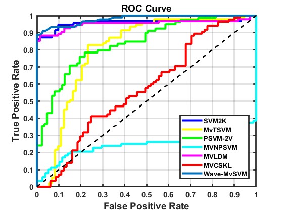
(b)

(c)

(d)

Figure 5: ROC curves of the proposed Wave-MvSVM model along with the baseline models on the UCI and KEEL datasets.

Figure 5 presents the ROC curve, demonstrating the superior performance of the proposed Wave-MvSVM model compared to the baseline models on the UCI and KEEL datasets. The ROC curve provides a detailed assessment of the model’s diagnostic capability by plotting the true positive rate against the false positive rate across different threshold settings. The area under the ROC curve (AUC) for the proposed Wave-MvSVM model is notably higher, reflecting a better trade-off between sensitivity and specificity. This higher AUC indicates that the wave-MvSVM model excels at distinguishing between positive and negative instances, leading to more precise predictions. The proposed Wave-MvSVM model enhances its ability to correctly identify true positives, thus minimizing false negatives and ensuring more dependable detection. These results highlight the robustness and effectiveness of the proposed Wave-MvSVM model in classification tasks, surpassing the performance of the baseline models.

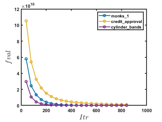
Figure 6: Convergence analysis of the proposed Wave-MvSVM model on monk_1, credit_approval, and cylinder_bands datasets. The horizontal axis represents the number of iterations, while the vertical axis denotes the value of the objective function

6.3 Convergence analysis

We examined the convergence of Wave-MvSVM on three benchmark datasets, namely monk_1, credit_approval, and cylinder_bands. The convergence analysis, depicted in Figure 6, illustrates that the objective function decreases monotonically with increasing iterations, stabilizing after approximately $200$ iterations. The examination revealed that the objective function consistently decreased with each iteration, indicating a steady and reliable path toward minimization. This continuous decline highlights the efficacy of the ADMM algorithm in optimizing the Wave-MvSVM model. From Figure 6, the rapid convergence observed, with the objective function stabilizing within approximately $200$ iterations, highlights the robustness and efficiency of the ADMM algorithm. Based on these findings, we conclude that it is both reasonable and appropriate to utilize the ADMM algorithm for solving Wave-MvSVM, ensuring efficient and reliable convergence of the objective function.

Table 2: Classification performance of proposed Wave-MvSVM model along with the baseline models on AwA datasets with the Gaussian kernel.

Dataset	SVM2K [10]	MvTSVM [37]	PSVM-2V [29]	MVNPSVM [30]	MVLDM [15]	MVCSKL [32]	Wave-MvSVM†
	$(C_{1},\sigma)$	$(C_{1},\sigma)$	$(C_{1},\gamma,\sigma)$	$(C_{1},D,\sigma)$	$(C_{1},v_{1},v_{2},\theta,\sigma)$	$(a_{1},d,\gamma,c_{1},\sigma)$	$(a_{1},\lambda,\mathcal{C}_{1},_{2},D,\sigma)$
Chimpanzee vs Persian cat	$77.5$	$68.33$	$70.83$	$70$	$\underline{86.11}$	$73.61$	88.53
	$(4,16)$	$(0.03125,32)$	$(0.03125,4,8)$	$(0.03125,0.1,1)$	$(0.5,0.25,4,0.25,0.25,4)$	$(0.1,0.25,0.25,0.25,0.25)$	$(2,0.6,0.25,0.25,2,0.5)$
Chimpanzee vs Pig	$\underline{72.50}$	$66.67$	$71.67$	$68.33$	$66.67$	$68.06$	72.88
	$(4,16)$	$(0.03125,4)$	$(1,0.25,1)$	$(0.125,0.2,1)$	$(0.25,0.25,0.25,0.25,0.25,2)$	$(1,2,2,2,4)$	$(2,0.8,0.25,0.25,2,0.5)$
Chimpanzee vs Giant panda	$63.33$	$62.5$	$68.33$	$66.67$	$\underline{72.22}$	$70.04$	74.14
	$(2,1)$	$(0.03125,1)$	$(0.0625,16,4)$	$(4,0.8,8)$	$(2,0.25,0.25,0.25,4,2)$	$(10,0.25,0.25,0.25,4)$	$(1,0.6,0.25,0.25,0.25,4)$
Chimpanzee vs Leopard	$70$	$69.17$	72.50	$69.83$	$68.75$	$70$	$\underline{72.22}$
	$(2,0.5)$	$(0.03125,32)$	$(0.03125,32,16)$	$(4,0.9,8)$	$(0.25,0.25,0.25,0.25,0.5,1)$	$(0.1,1,1,0.25,0.5)$	$(0,0.6,0.25,0.25,1,2)$
Chimpanzee vs Hippopotamus	$74.83$	$64.17$	$70.83$	$74.83$	$\underline{78.47}$	$76.39$	78.83
	$(2,32)$	$(0.03125,32)$	$(0.03125,2,1)$	$(32,0.8,1)$	$(0.5,0.5,0.25,0.25,0.5,2)$	$(0.1,0.25,0.25,0.25,0.25)$	$(0.5,0.8,0.25,0.25,0.25,4)$
Chimpanzee vs Rat	$70.17$	$69.67$	$70$	$70$	$68.06$	$\underline{70.83}$	70.89
	$(1,4)$	$(0.03125,32)$	$(0.03125,4,1)$	$(0.0625,0.1,1)$	$(1,1,0.25,0.25,1,1)$	$(1,0.5,0.5,4,4)$	$(0,0.6,0.25,0.25,2,2)$
Chimpanzee vs Seal	$71.33$	$70$	$71.17$	$70.17$	$75.69$	$\underline{81.94}$	85.42
	$(2,16)$	$(0.03125,32)$	$(1,0.25,1)$	$(0.125,0.2,2)$	$(0.25,0.25,0.25,0.25,0.25,2)$	$(1,2,2,2,4)$	$(0,0.8,0.25,0.25,2,0.5)$
Chimpanzee vs Humpback whale	$82.17$	$72.5$	$82.5$	$70.33$	$81.25$	$\underline{92.36}$	96.53
	$(4,2)$	$(0.03125,32)$	$(0.25,0.0625,2)$	$(0.03125,0.1,1)$	$(2,2,0.25,4,2,2)$	$(0.1,0.25,0.25,0.25,0.25)$	$(1,0.6,0.25,4,0.25,4)$
Chimpanzee vs Raccoon	$70.83$	$64.17$	$72.5$	$68.33$	$72.22$	$\underline{72.92}$	74.83
	$(4,32)$	$(0.03125,32)$	$(0.03125,1,2)$	$(8,0.9,4)$	$(4,4,0.25,0.25,4,2)$	$(1,4,4,0.25,4)$	$(0,0.8,4,0.25,1,4)$
Giant panda vs Leopard	$60.33$	$60.5$	$60.83$	$60.67$	$61.81$	79.86	$\underline{77.08}$
	$(4,1)$	$(0.03125,32)$	$(0.0625,16,2)$	$(8,0.9,4)$	$(1,2,2,4,0.25,1)$	$(1,0.25,0.25,4,0.25)$	$(0,0.8,0.25,0.25,0.5,4)$
Giant panda vs Persian cat	79.50	$76.67$	$76.67$	$\underline{79.17}$	$66.67$	$77.78$	$78.83$
	$(2,0.5)$	$(0.03125,32)$	$(2,8,2)$	$(0.0625,0.1,1)$	$(4,0.25,0.25,0.25,4,2)$	$(0.1,1,1,0.25,0.25)$	$(0,0.8,0.25,4,0.5,0.25)$
Giant panda vs Pig	$60.83$	$65$	$61.67$	$63.33$	$\underline{65.97}$	$57.64$	68.75
	$(2,0.5)$	$(8,32)$	$(0.5,0.25,1)$	$(0.0625,0.1,0.5)$	$(0.25,0.25,4,4,0.5,2)$	$(0.1,0.25,0.25,0.25,0.25)$	$(2,0.4,0.25,0.25,0.25,4)$
Giant panda vs Hippopotamus	$67.5$	$70$	78.33	$70.67$	$74.31$	$73.61$	$\underline{75.69}$
	$(1,1)$	$(0.03125,32)$	$(0.125,32,4)$	$(0.03125,0.1,0.5)$	$(1,0.5,0.25,0.25,4,4)$	$(0.1,0.25,0.25,0.25,0.25)$	$(0,0.2,0.25,0.25,1,0.25)$
Giant panda vs Humpback whale	$85.17$	$83.33$	$83.33$	$84.17$	$\underline{93.75}$	$92.36$	95.83
	$(8,32)$	$(0.03125,32)$	$(0.25,0.03125,1)$	$(0.03125,0.1,1)$	$(4,0.25,0.25,0.25,2,1)$	$(0.1,0.5,0.5,0.25,0.5)$	$(0,0.4,0.25,0.25,4,4)$
Giant panda vs Raccoon	$60.83$	$67.5$	$62.5$	$65.17$	$64.58$	$\underline{70.14}$	77.78
	$(4,8)$	$(0.03125,32)$	$(0.5,1,2)$	$(8,0.9,4)$	$(2,1,0.25,0.25,4,4)$	$(0.1,0.25,0.25,0.25,0.25)$	$(0,0.8,0.25,2,0.5,4)$
Giant panda vs Rat	$69.33$	$64.17$	$68.67$	$65.67$	$\underline{70.14}$	$64.58$	70.42
	$(2,1)$	$(0.03125,32)$	$(0.0625,4,2)$	$(0.0625,0.1,1)$	$(0.5,0.25,4,4,1,4)$	$(0.1,0.25,0.25,0.25,0.25)$	$(0.5,1,1,4,0.5,4)$
Giant panda vs Seal	$75$	$72$	$74.5$	$73.33$	86.81	$73.61$	$\underline{79.17}$
	$(2,1)$	$(0.03125,32)$	$(0.25,0.25,2)$	$(0.03125,0.1,0.5)$	$(1,0.5,0.25,0.25,2,1)$	$(0.1,2,2,0.25,0.25)$	$(2,0.8,0.25,0.25,0.25,4)$
Leopard vs Persian cat	$81.67$	$80$	$77.5$	$80$	$80.56$	$\underline{81.94}$	82.25
	$(8,8)$	$(0.03125,32)$	$(2,8,2)$	$(0.03125,0.1,0.5)$	$(2,0.25,0.25,0.25,4,1)$	$(0.1,2,2,0.25,0.25)$	$(0.5,0.2,0.25,0.25,0.25,4)$
Leopard vs Pig	$\underline{70}$	$66.67$	$63.33$	$67.5$	$68.75$	$65.97$	70.58
	$(2,0.5)$	$(0.03125,32)$	$(0.5,0.5,0.5)$	$(0.03125,0.1,0.25)$	$(1,0.25,0.25,0.25,2,0.5)$	$(0.1,0.25,0.25,0.25,0.25)$	$(0,0.4,0.25,0.25,0.25,4)$
Leopard vs Hippopotamus	$71.67$	$72.5$	$70$	$69.17$	$\underline{75}$	$70.83$	76.39
	$(1,1)$	$(0.03125,32)$	$(1,0.03125,1)$	$(0.03125,0.1,0.25)$	$(2,0.5,0.25,0.25,0.25,2)$	$(0.1,0.25,0.25,0.25,0.25)$	$(1.5,0.6,0.25,0.25,0.25,4)$
Leopard vs Humpback whale	$84.17$	$80$	$86.33$	$85.83$	$89.58$	$\underline{92.36}$	95.14
	$(4,0.5)$	$(0.03125,32)$	$(0.03125,8,2)$	$(0.03125,0.1,1)$	$(0.5,0.5,0.25,0.25,0.25,2)$	$(1,0.25,4,0.25,0.25)$	$(0,0.6,0.25,0.25,2,4)$
Leopard vs Raccoon	$62.5$	$64.17$	$60$	68.33	$56.94$	$\underline{66.67}$	$65.28$
	$(8,0.5)$	$(0.03125,32)$	$(0.03125,2,1)$	$(0.03125,0.1,0.125)$	$(4,1,0.25,0.25,1,2)$	$(0.1,0.25,0.25,0.25,0.25)$	$(0.5,0.4,0.25,0.25,0.5,4)$
Leopard vs Rat	$69.17$	76.67	$70$	$\underline{75.83}$	$65.28$	$65.28$	$70.83$
	$(1,0.5)$	$(0.03125,32)$	$(4,0.03125,2)$	$(0.03125,0.1,1)$	$(2,0.5,0.25,0.25,4,2)$	$(0.1,0.25,0.25,0.25,0.25)$	$(1.5,0.6,0.25,0.25,0.25,1)$
Leopard vs Seal	$70.83$	$68.33$	$67.5$	$70$	$81.25$	$\underline{82.64}$	84.03
	$(4,0.5)$	$(0.03125,32)$	$(0.5,1,2)$	$(0.03125,0.1,0.5)$	$(1,0.5,0.25,0.25,4,1)$	$(0.1,4,2,2,4)$	$(0.5,1,2,4,0.25,4)$
Persian cat vs Pig	$75.83$	$\underline{77.5}$	$73.33$	$\underline{77.5}$	$69.44$	$70.14$	78.36
	$(1,2)$	$(0.03125,32)$	$(8,0.03125,8)$	$(4,0.9,8)$	$(4,2,0.25,0.25,0.25,4)$	$(0.1,0.25,0.25,0.25,0.25)$	$(0.5,1,0.25,0.25,1,4)$
Persian cat vs Hippopotamus	$79.33$	$70$	$77.5$	$72.5$	$75.69$	$\underline{80.56}$	81.25
	$(2,1)$	$(0.03125,32)$	$(2,0.5,2)$	$(0.0625,0.9,2)$	$(2,0.25,0.25,0.25,2,4)$	$(1,0.25,0.25,1,0.25)$	$(0,0.4,0.25,0.25,0.25,2)$
Persian cat vs Humpback whale	$72.5$	$70.83$	$70.83$	$74.67$	$85.42$	89.58	$\underline{86.11}$
	$(1,1)$	$(0.03125,32)$	$(0.0625,0.125,2)$	$(0.0625,0.9,16)$	$(0.5,0.5,0.25,4,2,4)$	$(10,0.25,0.25,4,4)$	$(1,0.2,0.25,0.25,0.25,1)$
Persian cat vs Raccoon	$68.33$	$70.83$	$68.83$	$70.83$	$65.97$	$\underline{79.86}$	80.56
	$(4,1)$	$(0.03125,32)$	$(0.03125,0.03125,0.03125)$	$(16,0.9,2)$	$(4,0.25,0.25,0.25,1,1)$	$(10,0.25,2,0.5,4)$	$(0.5,0.8,2,4,0.25,2)$
Persian cat vs Rat	$\underline{62.50}$	$48.33$	$53.33$	$49.17$	$56.94$	$56.94$	65.28
	$(2,4)$	$(0.03125,32)$	$(8,4,8)$	$(4,0.9,8)$	$(0.5,1,0.25,0.25,0.25,4)$	$(0.1,1,4,0.5,4)$	$(1.5,1,0.25,0.25,0.25,1)$
Persian cat vs Seal	$82.5$	$70.83$	85.83	$75.83$	$\underline{83.33}$	$75$	$76.39$
	$(1,4)$	$(0.03125,32)$	$(0.25,0.03125,2)$	$(0.0625,0.9,4)$	$(0.5,0.25,0.25,0.25,0.5,2)$	$(0.1,0.25,0.25,0.25,4)$	$(1,0.8,0.25,4,0.25,4)$
Pig vs Hippopotamus	$64.17$	$67.5$	$68.33$	$68.33$	$\underline{72.22}$	$68.75$	74.58
	$(8,16)$	$(0.03125,0.03125)$	$(1,0.03125,8)$	$(0.03125,0.1,0.25)$	$(0.25,0.25,0.25,0.25,2,1)$	$(0.1,0.25,0.25,0.25,4)$	$(1.5,1,0.25,2,4,2)$
Pig vs Humpback whale	$85$	$82.5$	$87.5$	$85.83$	88.89	$\underline{87.50}$	88.89
	$(8,16)$	$(0.03125,32)$	$(0.0625,32,2)$	$(0.03125,0.1,0.5)$	$(1,0.25,0.25,0.25,0.25,4)$	$(10,0.25,0.25,0.25,4)$	$(0,0.4,0.25,0.25,0.25,4)$
Pig vs Raccoon	$60.83$	$55.83$	$55$	$48.33$	$\underline{62.50}$	$60.42$	72.22
	$(8,32)$	$(0.03125,0.03125)$	$(16,1,16)$	$(2,0.9,16)$	$(1,0.25,0.25,0.25,2,0.5)$	$(10,0.25,0.25,0.25,4)$	$(1.5,1,0.25,0.25,4,4)$
Pig vs Rat	$59.17$	$54.17$	$54.17$	$50.83$	64.58	$\underline{63.19}$	$52.78$
	$(2,2)$	$(0.03125,0.03125)$	$(0.125,1,2)$	$(0.03125,0.1,0.5)$	$(4,0.25,0.25,0.25,4,2)$	$(0.1,0.25,0.25,2,4)$	$(1.5,0.8,0.25,0.25,2,0.5)$
Pig vs Seal	$\underline{75}$	$71.67$	$69.17$	$72.67$	$72.92$	$72.22$	75.36
	$(2,1)$	$(0.03125,32)$	$(0.25,0.03125,2)$	$(0.03125,0.1,1)$	$(1,0.25,0.25,0.25,1,2)$	$(1,0.25,0.25,0.5,4)$	$(2,0.8,0.25,0.25,1,2)$
Hippopotamus vs Humpback whale	$77.5$	$74.17$	$78.33$	$75.83$	$\underline{79.86}$	$74.31$	81.25
	$(1,4)$	$(0.03125,32)$	$(0.25,8,4)$	$(0.03125,0.1,0.5)$	$(1,0.25,0.25,0.25,0.25,4)$	$(1,0.25,2,0.5,4)$	$(0.5,1,1,1,0.25,0.25)$
Hippopotamus vs Raccoon	$70.5$	$70.67$	$70.83$	$69.17$	75.69	$75$	$\underline{72.22}$
	$(4,8)$	$(0.03125,32)$	$(0.5,0.03125,1)$	$(0.0625,0.9,1)$	$(1,0.25,2,4,1,4)$	$(10,0.25,0.25,0.25,4)$	$(2,0.2,4,4,0.25,0.25)$
Hippopotamus vs Rat	$68.33$	$63.33$	$68$	$59.17$	$\underline{64.58}$	75.69	$60.42$
	$(1,0.5)$	$(0.03125,32)$	$(0.03125,2,2)$	$(0.03125,0.1,1)$	$(1,1,0.25,0.25,2,0.5)$	$(1,0.25,0.25,0.25,1)$	$(0,0.6,0.5,0.5,0.25,2)$
Hippopotamus vs Seal	$69.17$	$\underline{70.33}$	70.83	70.83	$60.42$	$67.36$	$68.06$
	$(2,0.5)$	$(0.03125,16)$	$(0.5,0.5,2)$	$(0.03125,0.1,0.5)$	$(2,2,4,4,0.25,4)$	$(0.1,2,4,0.25,4)$	$(0,0.6,0.5,0.5,1,4)$
Humpback whale vs Raccoon	$80.67$	$74.17$	$80.17$	$80$	$83.33$	91.67	$\underline{88.89}$
	$(4,2)$	$(0.03125,32)$	$(2,0.03125,2)$	$(4,0.5,4)$	$(1,0.5,0.25,0.25,0.5,2)$	$(0.1,0.25,0.25,1,4)$	$(1.5,0.4,0.25,0.25,0.25,0.25)$
Humpback whale vs Rat	80	$78.17$	80	$\underline{79.17}$	$77.78$	$75.69$	80
	$(2,2)$	$(0.03125,32)$	$(0.03125,16,8)$	$(8,0.9,4)$	$(1,0.5,0.25,2,0.25,0.5)$	$(1,0.25,0.25,0.25,2)$	$(1,0.4,0.25,0.25,0.25,0.25)$
Humpback whale vs Seal	$75$	$76.67$	$77.5$	$74.67$	$\underline{78.47}$	$74.31$	79.44
	$(1,1)$	$(2,32)$	$(2,0.03125,8)$	$(8,0.9,4)$	$(2,0.5,0.25,0.25,0.5,4)$	$(0.1,0.25,0.25,0.25,1)$	$(1,0.8,0.25,0.25,0.25,0.25)$
Raccoon vs Rat	$71.33$	72.5	$59.17$	$\underline{71.67}$	$65.28$	$54.17$	$61.81$
	$(2,0.5)$	$(0.03125,32)$	$(0.03125,2,2)$	$(0.0625,0.1,1)$	$(0.25,1,0.25,0.25,0.25,4)$	$(1,2,4,0.25,2)$	$(1,0.8,0.25,0.25,0.25,0.25)$
Raccoon vs Seal	$72.5$	$68.33$	$71.67$	$71.67$	$75.69$	$\underline{77.78}$	80.56
	$(1,2)$	$(0.03125,32)$	$(0.5,0.03125,2)$	$(0.03125,0.1,1)$	$(1,0.5,0.25,0.25,0.25,4)$	$(0.1,0.25,0.25,0.25,1)$	$(0,0.6,0.25,0.25,0.25,1)$
Rat vs Seal	$65$	$60$	$64.17$	$66.67$	$\underline{69.87}$	75.69	$65.28$
	$(2,1)$	$(0.03125,32)$	$(0.03125,32,16)$	$(0.0625,0.9,2)$	$(0.5,0.25,0.25,4,0.5,8)$	$(1,0.25,4,0.25,4)$	$(1.5,1,2,4,0.25,4)$
Average ACC	$71.92$	$69.4$	$71.02$	$70.5$	$73.33$	$\underline{74.16}$	76.71
Average Rank	$4.11$	$5.51$	$4.50$	$4.78$	$3.62$	$\underline{3.60}$	1.88
† represents the proposed models.
The boldface and underline indicate the best and second-best models, respectively, in terms of ACC.

6.4 Experiments on AwA datasets

In this subsection, we perform a detailed analysis by comparing the proposed Wave-MvSVM model with baseline models using the AwA dataset. This dataset consists of 30,475 images from 50 animal classes, with each image represented by six pre-extracted features. For our evaluation, we focus on ten test classes: chimpanzee, Persian cat, leopard, raccoon, humpback whale, giant panda, pig, hippopotamus, seal, and rat, amounting to a total of $6,180$ images. The $2000$-dimensional $L_{1}$ normalized Speeded-Up Robust Features (SURF) are denoted as view 1, while the $252$-dimensional Histogram of Oriented Gradient (HOG) feature descriptors are represented as view 2. We employ a one-against-one strategy for each combination of class pairs to train $45$ binary classifiers. We evaluate the performance of the proposed Wave-MvSVM model along with the baseline models using ACC metrics and corresponding optimal hyperparameters, which are reported in Table 2. The average ACC of the proposed Wave-MvSVM and the baseline SVM2K, MvTSVM, PSVM-2V, MVNPSVM, MVLDM, and MVCSKL models are $76.71\%$, $71.92\%$, $69.40\%$, $71.02\%$, $70.50\%$, $73.33\%$, and $74.16\%$, respectively. Table 2 presents the average rank of the proposed Wave-MvSVM and the baseline models. The proposed Wave-MvSVM model achieves the highest average ACC, the lowest average rank, and the most wins, demonstrating their superior performance. Now, we conduct the Friedman statistical test, followed by the Nemenyi post hoc tests. For the significance level of $\alpha=0.05$, we calculated as $\chi_{F}^{2}=76.65$ and $F_{F}=17.44$. The tabulated value is obtained by $F_{F}(6,264)=2.133$. The null hypothesis is rejected as $17.44>F_{F}(6,264)$. Now, the Nemenyi post-hoc test is employed to identify significant differences among the pairwise comparisons of the models. We calculate $C.D.=1.34$, which indicates that the average rankings of the models in Table 2 should have a minimum difference of $1.34$ to be considered statistically significant. The differences in average ranks between the proposed Wave-MvSVM and the baseline SVM2K, MvTSVM, PSVM-2V, MVNPSVM, MVLDM, and MVCSKL models are $2.23$, $3.63$, $2.62$, $2.90$, $1.74$, and $1.72$. The observed differences are greater than the critical difference $C.D.$. Consequently, based on the Nemenyi post hoc test, significant distinctions are found between the proposed Wave-MvSVM model and the baseline models SVM2K, MvTSVM, PSVM-2V, MVNPSVM, MVLDM, and MVCSKL. Consequently, the proposed Wave-MvSVM model demonstrates superior performance compared to baseline models. Considering the above discussion based on ACC, rank, and statistical tests, we can conclude that the proposed Wave-MvSVM model demonstrates superior and robust performance compared to the baseline models.

Table 3: Classification performance of proposed Wave-MvSVM model along with the baseline models on UCI and KEEL datasets with label noise.

Dataset	Noise	SVM2K [10]	MvTSVM [37]	PSVM-2V [29]	MVNPSVM [30]	MVLDM [15]	MVCSKL [32]	Wave-MvSVM†
		$(C_{1},\sigma)$	$(C_{1},\sigma)$	$(C_{1},\gamma,\sigma)$	$(C_{1},D,\sigma)$	$(C_{1},v_{1},v_{2},\theta,\sigma)$	$(a_{1},d,\gamma,c_{1},\sigma)$	$(a_{1},\lambda,\mathcal{C}_{1},_{2},D,\sigma)$
blood	$5\%$	$75$	77.68	$\underline{77.23}$	$73.49$	77.68	$72.06$	77.68
		$(2,0.5)$	$(0.03125,32)$	$(0.03125,32,16)$	$(4,0.9,8)$	$(0.25,0.25,0.25,0.25,0.5,1)$	$(0.1,1,1,0.25,0.5)$	$(0,0.6,0.25,0.25,1,2)$
	$10\%$	$\underline{79.46}$	$77.23$	$77.23$	$61.91$	$77.23$	$77.68$	79.68
		$(2,0.5)$	$(8,32)$	$(0.5,0.25,1)$	$(0.0625,0.1,0.5)$	$(0.25,0.25,4,4,0.5,2)$	$(0.1,0.25,0.25,0.25,0.25)$	$(2,0.4,0.25,0.25,0.25,4)$
	$15\%$	$\underline{77.23}$	$\underline{77.23}$	$\underline{77.23}$	$74.1$	$\underline{77.23}$	$76.34$	78.87
		$(2,0.5)$	$(0.03125,32)$	$(0.5,0.5,0.5)$	$(0.03125,0.1,0.25)$	$(1,0.25,0.25,0.25,2,0.5)$	$(0.1,0.25,0.25,0.25,0.25)$	$(0,0.4,0.25,0.25,0.25,4)$
	$20\%$	$76.79$	$77.68$	$75.89$	$66.17$	$\underline{78.57}$	$72.77$	81.43
		$(2,4)$	$(0.03125,32)$	$(8,4,8)$	$(4,0.9,8)$	$(0.5,1,0.25,0.25,0.25,4)$	$(0.1,1,4,0.5,4)$	$(1.5,1,0.25,0.25,0.25,1)$
Average ACC		$77.12$	$77.46$	$76.9$	$68.92$	$\underline{77.68}$	$74.71$	79.42
breast_cancer_wisc_prog	$5\%$	$71.36$	$76.27$	$76.27$	$60.66$	$74.58$	$\underline{77.97}$	78.02
		$(8,32)$	$(0.03125,32)$	$(0.25,0.03125,1)$	$(0.03125,0.1,1)$	$(4,0.25,0.25,0.25,2,1)$	$(0.1,0.5,0.5,0.25,0.5)$	$(0,0.4,0.25,0.25,4,4)$
	$10\%$	$71.19$	77.97	$\underline{79.66}$	$73.31$	$76.27$	$74.41$	$79.41$
		$(1,1)$	$(0.03125,32)$	$(1,0.03125,1)$	$(0.03125,0.1,0.25)$	$(2,0.5,0.25,0.25,0.25,2)$	$(0.1,0.25,0.25,0.25,0.25)$	$(1.5,0.6,0.25,0.25,0.25,4)$
	$15\%$	$76.27$	81.36	$72.94$	$74.45$	$\underline{80.75}$	$71.19$	$80.71$
		$(4,0.5)$	$(0.03125,32)$	$(0.5,1,2)$	$(0.03125,0.1,0.5)$	$(1,0.5,0.25,0.25,4,1)$	$(0.1,4,2,2,4)$	$(0.5,1,2,4,0.25,4)$
	$20\%$	$74.58$	$72.88$	$74.58$	$60.69$	$\underline{74.75}$	$73.53$	76.67
		$(2,1)$	$(0.03125,32)$	$(0.03125,32,16)$	$(0.0625,0.9,2)$	$(0.5,0.25,0.25,4,0.5,8)$	$(1,0.25,4,0.25,4)$	$(1.5,1,2,4,0.25,4)$
Average ACC		$73.35$	$\underline{77.12}$	$75.86$	$67.28$	$76.59$	$74.28$	78.7
brwisconsin	$5\%$	$80.69$	$81.24$	$\underline{82.65}$	$81.19$	$82.31$	$79.78$	83.82
		$(1,0.5)$	$(2,16)$	$(0.125,0.5,1)$	$(0.25,0.1,32)$	$(1,1,0.25,0.25,1)$	$(0.1,0.25,0.25,0.25,0.25)$	$(0,0.2,0.25,0.25,0.25,0.25)$
	$10\%$	$75.98$	$71.76$	$73.14$	79.92	$\underline{79.9}$	$74.31$	$74.8$
		$(0.25,32)$	$(0.03125,4)$	$(4,0.5,32)$	$(0.03125,0.6,32)$	$(0.5,0.5,0.25,0.25,0.5)$	$(1,0.5,0.5,0.25,0.5)$	$(0,0.2,0.25,0.25,0.25,2)$
	$15\%$	76.96	$73.24$	$72.88$	$71.19$	$76.47$	$76.27$	$\underline{76.82}$
		$(0.5,32)$	$(16,32)$	$(0.5,0.03125,32)$	$(0.03125,0.1,0.03125)$	$(0.25,0.25,0.25,0.25,0.25)$	$(0.1,2,2,0.25,0.25)$	$(0,0.2,0.5,4,0.25,0.25)$
	$20\%$	$75$	$\underline{79.22}$	$76.76$	$72$	$75.29$	$71.37$	79.9
		$(0.03125,0.03125)$	$(0.03125,0.03125)$	$(0.03125,0.03125,1)$	$(2,0.1,32)$	$(0.25,0.25,0.25,0.25,0.25)$	$(1,0.25,0.25,0.25,0.25)$	$(0.5,1,1,0.25,0.25,1)$
Average ACC		$77.16$	$76.37$	$76.36$	$76.08$	$\underline{78.49}$	$75.43$	78.84
congressional_voting	$5\%$	$\underline{63.08}$	$62.31$	$62.31$	$60.66$	65.81	$62.95$	$60.42$
		$(1,16)$	$(0.03125,16)$	$(1,0.125,32)$	$(0.03125,0.3,32)$	$(0.25,0.25,0.25,0.25,0.25)$	$(0.1,2,2,0.25,2)$	$(1.5,0.8,0.25,0.25,0.25,0.25)$
	$10\%$	60.77	60.77	60.77	$57.61$	$\underline{57.69}$	$56.92$	$54.21$
		$(16,32)$	$(0.03125,2)$	$(0.03125,2,2)$	$(0.03125,0.1,0.03125)$	$(0.25,0.25,0.25,0.25,0.25)$	$(10,0.5,0.5,0.25,2)$	$(1.5,1,2,4,4,0.25)$
	$15\%$	$62.31$	$64.62$	69.09	$64.27$	$63.08$	$\underline{68.46}$	$67.97$
		$(2,1)$	$(0.03125,2)$	$(4,0.03125,4)$	$(0.03125,0.1,0.03125)$	$(0.25,0.25,0.25,0.25,0.25)$	$(0.1,1,1,0.25,0.25)$	$(1,0.2,0.5,0.25,0.25,4)$
	$20\%$	$61.54$	$\underline{63.08}$	64.62	$59.08$	$58.46$	$59.42$	$59.37$
		$(2,0.25)$	$(0.03125,32)$	$(8,0.25,4)$	$(1,0.9,8)$	$(4,4,0.25,4,4)$	$(0.1,0.5,0.5,0.25,0.25)$	$(2,1,0.25,0.25,0.25,0.5)$
Average ACC		$61.93$	$\underline{62.7}$	64.2	$60.41$	$61.26$	$61.94$	$60.49$
credit_approval	$5\%$	$75.36$	$74.11$	$76.96$	$\underline{77.7}$	$74.06$	$76.21$	78.25
		$(4,32)$	$(0.03125,16)$	$(4,0.03125,16)$	$(0.25,0.9,32)$	$(0.25,0.25,0.25,0.25,0.25)$	$(0.1,0.25,0.25,0.25,4)$	$(0,0.8,0.5,0.25,0.25,4)$
	$10\%$	$70.05$	$74.4$	$69.37$	$71.31$	75.51	$70.97$	$\underline{75.22}$
		$(16,1)$	$(0.03125,0.25)$	$(1,0.03125,1)$	$(16,0.9,16)$	$(2,2,0.25,0.25,2)$	$(1,0.25,0.25,0.25,0.25)$	$(0,0.2,1,0.25,0.25,1)$
	$15\%$	$61.84$	$64.4$	$66.3$	$63.61$	$\underline{68.74}$	$65.81$	69.25
		$(16,0.125)$	$(0.5,32)$	$(0.03125,0.03125,0.03125)$	$(1,0.4,8)$	$(2,0.25,0.25,4,0.25)$	$(0.1,2,0.25,0.25,4)$	$(0.5,0.2,4,0.25,0.25,4)$
	$20\%$	$68.6$	$69.28$	$62.61$	$68.51$	$\underline{76.33}$	$73.08$	77.19
		$(4,4)$	$(0.03125,32)$	$(0.5,0.03125,4)$	$(0.5,0.9,32)$	$(0.25,0.25,0.25,0.25,0.25)$	$(0.1,2,2,0.25,0.25)$	$(2,0.8,0.5,0.25,0.25,4)$
Average ACC		$68.96$	$70.55$	$68.81$	$70.28$	$\underline{73.66}$	$71.52$	74.98
Overall average ACC		$71.70$	$72.84$	$72.42$	$68.59$	$\underline{73.54}$	$71.58$	74.49
† represents the proposed models.
The boldface and underline indicate the best and second-best models, respectively, in terms of ACC.

6.5 Evaluation on UCI and KEEL datasets with added label noise

The UCI and KEEL datasets used in our evaluation reflect real-world scenarios. However, it is crucial to acknowledge that data impurities or noise can arise from various factors. In these situations, it is vital to create a robust model capable of managing such challenges effectively. To demonstrate the efficacy of the proposed Wave-MvSVM model under adverse conditions, we intentionally introduced label noise into selected datasets. For our comparative analysis, we chose five diverse datasets: blood, breast_cancer_wisc_prog, brwisconsin, congressional_voting, and credit_approval. We selected one dataset with the proposed Wave-MvSVM model to ensure impartiality in evaluating the models. To carry out a thorough analysis, we introduced label noise at varying levels of $5\%$, $10\%$, $15\%$, and $20\%$ to corrupt the labels. The average accuracies of all the models for the selected datasets with $5\%$, $10\%$, $15\%$, and $20\%$ noise levels are presented in Table 3. The average ACC of the proposed Wave-MvSVM model on blood with various noise levels is $79.42\%$, surpassing the performance of the baseline models. The ACC at $20\%$ level of noise is $81.43\%$, which surpasses at $0\%$ level of noise. On the breast_cancer_wisc_prog dataset, the average ACC of the proposed Wave-MvRVFl model is $78.70\%$, which secured the top position comparison to the baseline models. However, on the congressional_voting dataset, the proposed models did not achieve the top performance compared to the baseline models. Nonetheless, they did secure the top position at the $0\%$ level of noise with an ACC of $66.23\%$. On brwisconsin, and credit_approval datasets, the proposed models show the best performance with an average ACC of $78.84\%$, and $74.98\%$, respectively. On various levels of noise, the proposed Wave-MvSVM achieved an overall average ACC of $74.49\%$, surpassing all the baseline models. These results highlight the significance of the proposed Wave-MvSVM model as a robust solution capable of performing effectively in challenging environments marked by noise and impurities.

6.6 Sensitivity analysis

In this section, we perform the sensitivity analysis of several key hyperparameters of the proposed Wave-MvSVM model. These analyses covered various factors, including hyperparameters corresponding to the W-loss function $\lambda$ and $a$, discussed in subsection 6.6.1. We examined the effects of different levels of label noise in subsection 6.6.2. Finally, we assess the influence of hyperparameters $\mathcal{C}_{1}$ and $\mathcal{C}_{2}$, discussed in subsection 6.6.3.

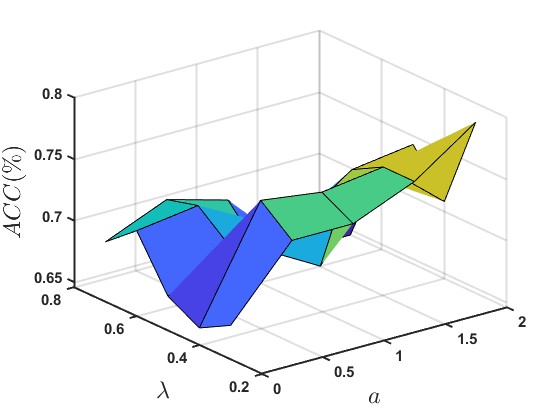
(a)

(b)

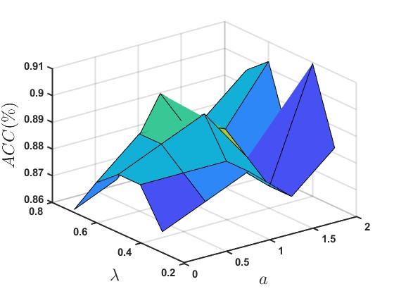
(c)

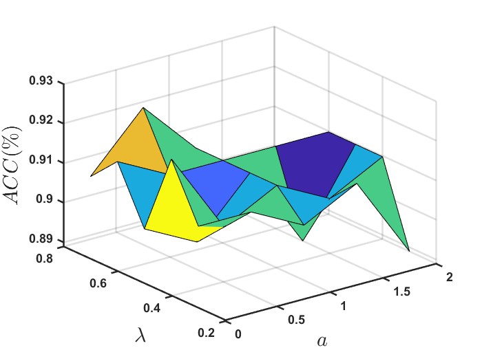
(d)

Figure 7: Effect of parameters of W-loss function $\lambda$ and $a$ on the performance of the proposed Wave-MvSVM model on AwA datasets.

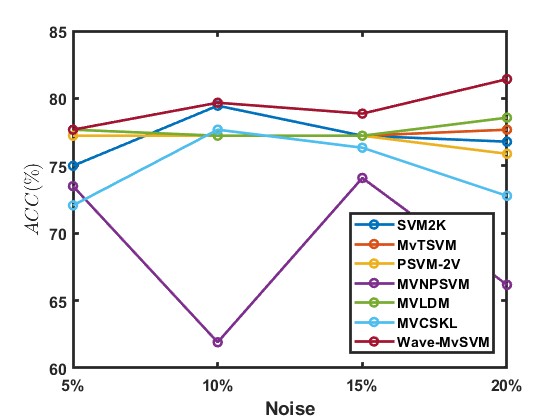
(a)

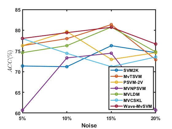
(b)

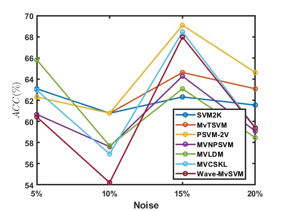
(c)

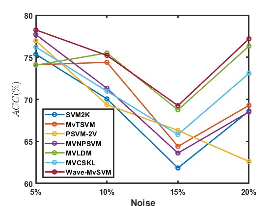
(d)

Figure 8: Effect of different levels of label noise on the performance of the proposed Wave-MvRVFL model on UCI and KEEL datasets.

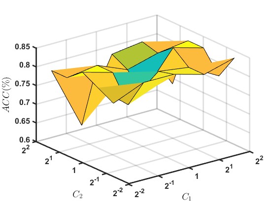
(a)

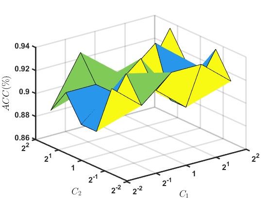
(b)

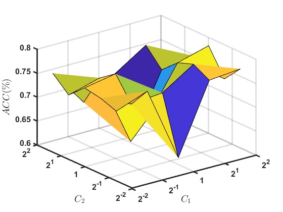
(c)

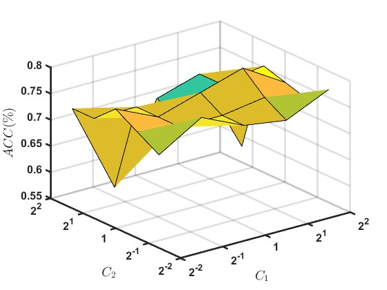
(d)

Figure 9: Effect of parameters $\mathcal{C}_{1}$ and $\mathcal{C}_{2}$ on the performance of the proposed Wave-MvSVM model on UCI and KEEL datasets.

6.6.1 Sensitivity analysis of W-loss parameters $\lambda$ and $a$

To thoroughly understand the robustness of the W-loss function, it is essential to analyze its sensitivity to the hyperparameters $\lambda$ and $a$. This thorough exploration enables us to identify the configuration that maximizes predictive ACC and enhances the model’s resilience when confronted with unseen data. Figure 7 illustrates a significant fluctuation in the model’s ACC across various $\lambda$ and $a$ values, underscoring the sensitivity of our model’s performance to these specific hyperparameters. From Figures 7(a) and 7(c), it is observed that the optimal performance of the proposed Wave-MvSVM model is within the $\lambda$ and $a$ ranges of $0.2$ to $0.6$ and $1$ to $2$, respectively. Similarly, from Figures 7(b) and 7(d), the ACC of the proposed Wave-MvSVM model achieves the maximum when $\lambda$ and $a$ range from $0.4$ to $0.8$, and $0$ to $1.5$ respectively. Therefore, we recommend utilizing $\lambda$ and $a$ from the range $0.2$ to $0.6$, and $0.5$ to $1.5$ for optimal results, although fine-tuning may be necessary depending on the dataset’s characteristics to achieve optimal generalization performance for the proposed Wave-MvSVM model.

6.6.2 Sensitivity analysis of label noise

One of the main focus of the proposed Wave-MvSVM model is to mitigate the adverse impact of noise. To thoroughly evaluate the robustness of the Wave-MvSVM model, we introduced label noise into four datasets: blood, breast_cancer_wisc_prog, planning, and monks_1. We varied the noise levels at $5\%$, $10\%$, $15\%$, and $20\%$. Figure 8 provides a detailed analysis of the results. It clearly shows that the performance of baseline models fluctuates significantly and tends to decline as the level of label noise increases. This instability indicates a susceptibility to noise, which can severely affect their classification ACC. In contrast, the Wave-MvSVM model consistently maintains superior performance across all levels of introduced noise. This stability demonstrates the model’s robustness and effectiveness in handling noisy data. The Wave-MvSVM’s ability to mitigate the effects of noise ensures reliable performance and ACC, even in challenging environments where data impurities are prevalent.

6.6.3 Sensitivity analysis of hyperparameter $C_{1}$ and $\mathcal{C}_{2}$

We delve into the impact of hyperparameters $\mathcal{C}_{1}$ and $\mathcal{C}_{2}$ on the predictive capability of the proposed Wave-MvSVM model. The sensitivity analysis, depicted in Figure 9, is conducted on both KEEL and UCI datasets, evaluating ACC variations with varying values of $\mathcal{C}_{1}$ and $\mathcal{C}_{2}$. However, beyond a certain threshold, further increments in $\mathcal{C}_{1}$ yield diminishing returns in testing ACC. Specifically, once the values surpass $2^{1}$, the ACC reaches a plateau, indicating that additional increases in $\mathcal{C}_{1}$ do not significantly enhance performance. This underscores the importance of meticulous hyperparameter selection for the proposed Wave-MvSVM model to achieve optimal generalization performance. By carefully tuning $\mathcal{C}_{1}$ and $\mathcal{C}_{2}$, practitioners can ensure the models’ effectiveness in handling diverse datasets and achieving robust predictive capabilities.

7 Conclusions and Future Work

In this paper, we propose a novel multiview support vector machine framework leveraging the wave loss function (Wave-MvSVM). It addresses the complexities of multi-view representations and handles noisy samples simultaneously within a unified framework. In line with the consensus and complementarity principles, Wave-MvSVM integrates a consensus regularization term and a combination weight strategy to enhance the utilization of multi-view representations effectively. The wave loss (W-loss) function, known for its smoothness, asymmetry, and bounded properties, proves highly effective in mitigating the detrimental impacts of noisy and outlier data, thereby improving model stability. The theoretical foundation supported by Rademacher’s complexity underscores its strong generalization capabilities of the proposed Wave-MvSVM model. We utilize the ADMM and GD algorithms to solve the optimization problem of the Wave-MvSVM model. To showcase the effectiveness, robustness, and efficiency of the proposed Wave-MvSVM model, we conducted a series of rigorous experiments and subjected them to thorough statistical analyses. We conducted experiments using datasets from UCI, KEEL, and AwA. The experimental findings, supported by statistical analyses, demonstrate that the proposed Wave-MvSVM models outperform baseline models in terms of generalization performance even when tested with datasets containing introduced label noise. In the future, one can extend the proposed Wave-MvSVM to handle scenarios with multiple views (more than two views) and develop specific acceleration strategies tailored for large-scale datasets. Additionally, exploring the integration of the asymmetric and bounded loss function into deep learning frameworks represents a meaningful and intriguing avenue for future research.

References

- Akhtar et al. [2023] Mushir Akhtar, M. Tanveer, and Mohd Arshad. RoBoSS: A robust, bounded, sparse, and smooth loss function for supervised learning. arXiv preprint arXiv:2309.02250, 2023.
- Akhtar et al. [2024, https://doi.org/10.1016/j.patcog.2024.110637] Mushir Akhtar, M. Tanveer, Mohd Arshad, and Alzheimer’s Disease Neuroimaging Initiative. Advancing supervised learning with the wave loss function: A robust and smooth approach. Pattern Recognition, page 110637, 2024, https://doi.org/10.1016/j.patcog.2024.110637.
- Bartlett and Mendelson [2002] Peter L Bartlett and Shahar Mendelson. Rademacher and Gaussian complexities: Risk bounds and structural results. Journal of Machine Learning Research, 3(Nov):463–482, 2002.
- Bartlett et al. [2006] Peter L Bartlett, Michael I Jordan, and Jon D McAuliffe. Convexity, classification, and risk bounds. Journal of the American Statistical Association, 101(473):138–156, 2006.
- Cortes and Vapnik [1995] Corinna Cortes and Vladimir Vapnik. Support-vector networks. Machine Learning, 20:273–297, 1995.
- Demšar [2006] Janez Demšar. Statistical comparisons of classifiers over multiple data sets. The Journal of Machine Learning Research, 7:1–30, 2006.
- Derrac et al. [2015] J Derrac, S Garcia, L Sanchez, and F Herrera. KEEL data-mining software tool: Data set repository, integration of algorithms and experimental analysis framework. J. Mult. Valued Log. Soft Comput, 17:255–287, 2015.
- Dinuzzo and Schölkopf [2012] Francesco Dinuzzo and Bernhard Schölkopf. The representer theorem for Hilbert spaces: a necessary and sufficient condition. Advances in Neural Information Processing Systems, 25, 2012.
- Dua and Graff [2017] Dheeru Dua and Casey Graff. UCI machine learning repository. Available: http://archive.ics.uci.edu/ml, 2017.
- Farquhar et al. [2005] Jason Farquhar, David Hardoon, Hongying Meng, John Shawe-Taylor, and Sandor Szedmak. Two view learning: SVM-2K, theory and practice. Advances in Neural Information Processing Systems, 18, 2005.
- Friedman [1937] Milton Friedman. The use of ranks to avoid the assumption of normality implicit in the analysis of variance. Journal of the American Statistical Association, 32(200):675–701, 1937.
- Fu et al. [2022] Haitao Fu, Feng Huang, Xuan Liu, Yang Qiu, and Wen Zhang. MVGCN: data integration through multi-view graph convolutional network for predicting links in biomedical bipartite networks. Bioinformatics, 38(2):426–434, 2022.
- Gupta et al. [2020] Akshansh Gupta, Riyaj Uddin Khan, Vivek Kumar Singh, M. Tanveer, Dhirendra Kumar, Anirban Chakraborti, and Ram Bilas Pachori. A novel approach for classification of mental tasks using multiview ensemble learning (MEL). Neurocomputing, 417:558–584, 2020.
- Hou et al. [2024] Zhaojie Hou, Jingjing Tang, Yan Li, Saiji Fu, and Yingjie Tian. MVQS: Robust multi-view instance-level cost-sensitive learning method for imbalanced data classification. Information Sciences, 675:120467, 2024.
- Hu et al. [2024, doi: 10.1109/TNNLS.2023.3349142] Kun Hu, Yingyuan Xiao, Wenguang Zheng, Wenxin Zhu, and Ching-Hsien Hsu. Multiview large margin distribution machine. IEEE Transactions on Neural Networks and Learning Systems, 2024, doi: 10.1109/TNNLS.2023.3349142.
- Huang et al. [2016] Chengquan Huang, Fu-lai Chung, and Shitong Wang. Multi-view L2-SVM and its multi-view core vector machine. Neural Networks, 75:110–125, 2016.
- Kumari et al. [2024] Anuradha Kumari, Mushir Akhtar, M. Tanveer, and Mohd Arshad. Diagnosis of breast cancer using flexible pinball loss support vector machine. Applied Soft Computing, 157:111454, 2024.
- Li et al. [2018] Yifeng Li, Fang-Xiang Wu, and Alioune Ngom. A review on machine learning principles for multi-view biological data integration. Briefings in Bioinformatics, 19(2):325–340, 2018.
- Long et al. [2022] Ting Long, Yutong Xie, Xianyu Chen, Weinan Zhang, Qinxiang Cao, and Yong Yu. Multi-view graph representation for programming language processing: An investigation into algorithm detection. In Proceedings of the AAAI Conference on Artificial Intelligence, volume 36, pages 5792–5799, 2022.
- Luo et al. [2020] Keyang Luo, Tao Guan, Lili Ju, Yuesong Wang, Zhuo Chen, and Yawei Luo. Attention-aware multi-view stereo. In Proceedings of the IEEE/CVF Conference on Computer Vision and Pattern Recognition, pages 1590–1599, 2020.
- Meng et al. [2020] Min Meng, Mengcheng Lan, Jun Yu, and Jigang Wu. Multiview consensus structure discovery. IEEE Transactions on Cybernetics, 52(5):3469–3482, 2020.
- Pisner and Schnyer [2020, https://doi.org/10.1016/B978-0-12-815739-8.00006-7] Derek A Pisner and David M Schnyer. Support vector machine. In Machine learning, pages 101–121. Elsevier, 2020, https://doi.org/10.1016/B978-0-12-815739-8.00006-7.
- Quadir and Tanveer [2024, 10.1109/TCSS.2024.3411395] A. Quadir and M. Tanveer. Granular Ball Twin Support Vector Machine With Pinball Loss Function. IEEE Transactions on Computational Social Systems, 2024, 10.1109/TCSS.2024.3411395.
- Sadr et al. [2020] Hossein Sadr, Mir Mohsen Pedram, and Mohammad Teshnehlab. Multi-view deep network: a deep model based on learning features from heterogeneous neural networks for sentiment analysis. IEEE Access, 8:86984–86997, 2020.
- Serra et al. [2024, https://doi.org/10.1016/B978-0-12-815480-9.00013-X] Angela Serra, Paola Galdi, and Roberto Tagliaferri. Multiview learning in biomedical applications. In Artificial Intelligence in the Age of Neural Networks and Brain Computing, pages 307–324. Elsevier, 2024, https://doi.org/10.1016/B978-0-12-815480-9.00013-X.
- Sun [2011] Shiliang Sun. Multi-view Laplacian support vector machines. In Advanced Data Mining and Applications: 7th International Conference, ADMA 2011, Beijing, China, December 17-19, 2011, Proceedings, Part II 7, pages 209–222. Springer, 2011.
- Sun and Shawe-Taylor [2010] Shiliang Sun and John Shawe-Taylor. Sparse semi-supervised learning using conjugate functions. Journal of Machine Learning Research, 11:2423–2455, 2010.
- Sun et al. [2018] Shiliang Sun, Xijiong Xie, and Chao Dong. Multiview learning with generalized eigenvalue proximal support vector machines. IEEE Transactions on Cybernetics, 49(2):688–697, 2018.
- Tang et al. [2017] Jingjing Tang, Yingjie Tian, Peng Zhang, and Xiaohui Liu. Multiview privileged support vector machines. IEEE Transactions on Neural Networks and Learning Systems, 29(8):3463–3477, 2017.
- Tang et al. [2018] Jingjing Tang, Dewei Li, Yingjie Tian, and Dalian Liu. Multi-view learning based on nonparallel support vector machine. Knowledge-Based Systems, 158:94–108, 2018.
- Tang et al. [2021] Jingjing Tang, Weiqi Xu, Jiahui Li, Yingjie Tian, and Shan Xu. Multi-view learning methods with the LINEX loss for pattern classification. Knowledge-Based Systems, 228:107285, 2021.
- Tang et al. [2023] Jingjing Tang, Zhaojie Hou, Xiaotong Yu, Saiji Fu, and Yingjie Tian. Multi-view cost-sensitive kernel learning for imbalanced classification problem. Neurocomputing, 552:126562, 2023.
- Tang et al. [2024, https://doi.org/10.1016/j.asoc.2024.111278] Jingjing Tang, Qingqing Yi, Saiji Fu, and Yingjie Tian. Incomplete multi-view learning: Review, analysis, and prospects. Applied Soft Computing, page 111278, 2024, https://doi.org/10.1016/j.asoc.2024.111278.
- Tian et al. [2022] Yingjie Tian, Shiding Sun, and Jingjing Tang. Multi-view teacher–student network. Neural Networks, 146:69–84, 2022.
- van Loon et al. [2020] Wouter van Loon, Marjolein Fokkema, Botond Szabo, and Mark de Rooij. Stacked penalized logistic regression for selecting views in multi-view learning. Information Fusion, 61:113–123, 2020.
- Wang et al. [2023] Huiru Wang, Jiayi Zhu, and Siyuan Zhang. Safe screening rules for multi-view support vector machines. Neural Networks, 166:326–343, 2023.
- Xie and Sun [2015] Xijiong Xie and Shiliang Sun. Multi-view twin support vector machines. Intelligent Data Analysis, 19(4):701–712, 2015.
- Xie and Sun [2019] Xijiong Xie and Shiliang Sun. Multi-view support vector machines with the consensus and complementarity information. IEEE Transactions on Knowledge and Data Engineering, 32(12):2401–2413, 2019.
- Xie and Sun [2020] Xijiong Xie and Shiliang Sun. General multi-view semi-supervised least squares support vector machines with multi-manifold regularization. Information Fusion, 62:63–72, 2020.
- Yan et al. [2022] Shen Yan, Xuehan Xiong, Anurag Arnab, Zhichao Lu, Mi Zhang, Chen Sun, and Cordelia Schmid. Multiview transformers for video recognition. In Proceedings of the IEEE/CVF Conference on Computer Vision and Pattern Recognition, pages 3333–3343, 2022.
- Ye et al. [2021] Xin Ye, Hongxia Dai, Lu-an Dong, and Xinyue Wang. Multi-view ensemble learning method for microblog sentiment classification. Expert Systems with Applications, 166:113987, 2021.
- Yu et al. [2011] Shi Yu, Leon Tranchevent, Xinhai Liu, Wolfgang Glanzel, Johan AK Suykens, Bart De Moor, and Yves Moreau. Optimized data fusion for kernel k-means clustering. IEEE Transactions on Pattern Analysis and Machine Intelligence, 34(5):1031–1039, 2011.
- Zhang et al. [2021] Weiwei Zhang, Guang Yang, Nan Zhang, Lei Xu, Xiaoqing Wang, Yanping Zhang, Heye Zhang, Javier Del Ser, and Victor Hugo C de Albuquerque. Multi-task learning with multi-view weighted fusion attention for artery-specific calcification analysis. Information Fusion, 71:64–76, 2021.
- Zhao et al. [2017] Jing Zhao, Xijiong Xie, Xin Xu, and Shiliang Sun. Multi-view learning overview: Recent progress and new challenges. Information Fusion, 38:43–54, 2017.
- Zhao and Bu [2022] Nan Zhao and Jie Bu. Robust multi-view subspace clustering based on consensus representation and orthogonal diversity. Neural Networks, 150:102–111, 2022.
- Zheng et al. [2019] Qinghai Zheng, Jihua Zhu, Zhongyu Li, Shanmin Pang, Jun Wang, and Yaochen Li. Feature concatenation multi-view subspace clustering. arXiv preprint arXiv:1901.10657, 2019.
- Zhu et al. [2022] Jiayi Zhu, Huiru Wang, Hongjun Li, and Qing Zhang. Fast multi-view twin hypersphere support vector machine with consensus and complementary principles. Applied Intelligence, 52(11):12684–12703, 2022.
- Zhuang et al. [2020] Xiaowei Zhuang, Zhengshi Yang, and Dietmar Cordes. A technical review of canonical correlation analysis for neuroscience applications. Human Brain Mapping, 41(13):3807–3833, 2020.