Plasma Equilibrium in Diamagnetic Trap with Neutral Beam Injection
Abstract
This paper presents a theoretical model of plasma equilibrium in the diamagnetic confinement mode in an axisymmetric mirror device with neutral beam injection. The hot ionic component is described within the framework of the kinetic theory, since the Larmor radius of the injected ions appears to be comparable to or even larger than the characteristic scale of the magnetic field inhomogeneity. The electron drag of the hot ions is taken into account, while the angular scattering due to ion-ion collisions is neglected. The background warm plasma, on the contrary, is considered to be in local thermal equilibrium, i.e. has a Maxwellian distribution function and is described in terms of magnetohydrodynamics. The density of the hot ions is assumed to be negligible compared to that of the warm plasma. Both the conventional gas-dynamic loss and the non-adiabatic loss specific to the diamagnetic confinement mode are taken into account. In this work, we do not consider the effects of the warm plasma rotation as well as the inhomogeneity of the electrostatic potential. A self-consistent theoretical model of the plasma equilibrium is constructed. In the case of the cylindrical bubble, this model is reduced to a simpler one. The numerical solutions in the limit of a thin transition layer of the diamagnetic bubble are found. Examples of the equilibria corresponding to the GDMT device are considered.
1 Introduction
Diamagnetic confinement, or diamagnetic bubble (Beklemishev, 2016; Khristo & Beklemishev, 2019, 2022; Kotelnikov, 2020; Chernoshtanov, 2020, 2022; Soldatkina et al., 2023), is a new operating mode designed to significantly enhance confinement in linear systems (Ivanov & Prikhodko, 2017; Dimov, 2005; Steinhauer, 2011b). The main idea of this regime is to form a high-pressure plasma bubble in the central part of a mirror device. Inside such a bubble, the plasma pressure reaches the equilibrium limit corresponding to , and the magnetic field tends to zero due to the plasma diamagnetism. The lifetime of the particles in the diamagnetic trap, i.e. the mirror device operating in the diamagnetic confinement mode, is estimated by Beklemishev (2016) in the framework of magnetohydrodynamics (MHD) as follows:
where is the lifetime in the gas-dynamic trap (GDT) (Ivanov & Prikhodko, 2017), and is the transverse transport time. Since plasma transport across the magnetic field in axisymmetric traps is usually far below axial losses: , a significantly enhanced overall confinement is expected in the diamagnetic trap: . In this regard, there is a practical interest in the experimental and theoretical study of this mode. In particular, one of the goals of the new generation linear machine Gas-Dynamic Multiple-Mirror Trap (GDMT) (Beklemishev et al., 2013; Bagryansky et al., 2019; Skovorodin et al., 2023) is to experimentally verify the concept of the diamagnetic confinement. In addition, the study of the diamagnetic regime is planned at the Compact Axisymmetric Toroid (CAT) (Bagryansky et al., 2016) currently operating at the Budker Institute of Nuclear Physics (Budker INP).
One can find a number of earlier theoretical works related to plasma confinement in open traps (see Grad, 1967; Newcomb, 1981; Lansky, 1993; Lotov, 1996; Kotelnikov et al., 2010; Kotelnikov, 2011). Effective confinement of plasma with in a gas-dynamic system was demonstrated experimentally in the 2MK-200 test facility by Zhitlukhin et al. (1984). High plasma confinement was also studied in the so-called magnetoelectrostatic traps (see Pastukhov, 1978, 1980; Ioffe et al., 1981; Pastukhov, 2021). Structures similar to the diamagnetic bubble, called magnetic holes, are often observed in space plasmas (see Kaufmann et al., 1970; Turner et al., 1977; Tsurutani et al., 2011; Kuznetsov et al., 2015).
The idea of diamagnetic confinement was originally proposed by Beklemishev (2016). The possibility of a discharge transition into the diamagnetic confinement mode is briefly discussed, and a stationary MHD model of a diamagnetic bubble equilibrium is constructed in the cylindrical approximation. Further, this hydrodynamic equilibrium model was extended by Khristo & Beklemishev (2019, 2022) to the case of a non-paraxial axisymmetric trap. In particular, diamagnetic bubble equilibria in the GDMT are computed, and the effect of magnetic field corrugation on equilibrium in a diamagnetic trap is studied. Beklemishev (2016) and Khristo & Beklemishev (2022) also briefly discuss the possibility of MHD stabilization by a combination of the vortex confinement (see Soldatkina et al., 2008; Beklemishev et al., 2010; Bagryansky et al., 2011) and the conducting wall (see Kaiser & Pearlstein, 1985; Berk et al., 1987; Kotelnikov et al., 2022).
As already noted, the magnetic field inside the diamagnetic bubble is close to zero. In this case, the Larmor radius and the mean free path of high-energy particles can be comparable to or even exceed the characteristic scale of magnetic field inhomogeneity, which is beyond the scope of MHD theory. Therefore, there is a need for a detailed kinetic model of fast particles in the diamagnetic trap. Research on the kinetic theory of the diamagnetic regime is already underway at the Budker INP. Kotelnikov (2020) constructed a fully kinetic equilibrium model in cylindrical geometry with a distribution function isotropic in the transverse plane inside the bubble. The collisionless dynamics of individual particles in a diamagnetic trap were studied by Chernoshtanov (2022). In addition, a particle-in-cell model for simulating high-pressure plasma in an open trap is currently being developed in the Budker INP by Kurshakov & Timofeev (2023). Work is also underway to create a code for numerical simulation of the diamagnetic regime (see Boronina et al., 2020; Efimova et al., 2020; Chernoshtanov et al., 2023, 2024).
Modern experiments on linear devices, such as the already mentioned GDMT and CAT, commonly involve the injection of high-energy (on the order of several tens of electronvolts) neutral beams to heat the plasma (Ivanov & Prikhodko, 2017; Belchenko et al., 2018). With this in mind, in the present paper, we aim to construct a theoretical model of diamagnetic bubble equilibrium in a gas-dynamic trap with neutral beam injection. The neutral beams are absorbed by the background plasma at a temperature much lower than the energy of the injected atoms. For this reason, to describe the equilibrium in such a system, we assume the plasma to consist of two fractions: the background warm plasma and the hot ions resulting from the neutral beam injection. The former is considered to be in local thermodynamic equilibrium and is described in terms of MHD; we take as a basis the hydrodynamic model constructed in the earlier works (Beklemishev, 2016; Khristo & Beklemishev, 2019, 2022). The hot ions, on the contrary, are assumed to have a non-Maxwellian distribution function and are described within the framework of the kinetic theory. Similar hybrid equilibria were considered earlier in application to field reversed configurations (FRCs) (Rostoker & Qerushi, 2002; Qerushi & Rostoker, 2002a, b, 2003; Steinhauer, 2011a).
For simplicity, we consider the approximation of a long, axisymmetric diamagnetic trap. In this case, in the absence of dissipation and scattering, the azimuthal angular momentum and the total energy of a single charged particle are conserved. At the same time, since the magnetic field in the diamagnetic confinement regime has considerable gradients, the magnetic moment is not globally conserved. However, it was shown independently by Chernoshtanov (2020, 2022) and Kotelnikov (2020) that in a diamagnetic trap, the adiabatic invariant can be conserved under specific conditions. In addition, it is known that in such axisymmetric systems there is a region in phase space where particles are absolutely confined (see Morozov & Solov’ev, 1966; Lovelace et al., 1978; Larrabee et al., 1979; Hsiao & Miley, 1985).
In the present paper, we assume the hot ions to be injected into the region of the phase space, where, first, the absolute confinement criterion is met and, second, the condition of the adiabaticity is violated. The former saves us from solving the complex problem of taking into account the hot ion loss. The latter leads to the distribution function of the hot ions being homogeneous on the hypersurface of the constant azimuthal angular momentum and total energy, and hence not depending on the adiabatic invariant . Violation of the adiabaticity occurs typically due to the non-paraxial ends of the bubble configuration (Beklemishev, 2016). We also assume the energy of the hot ions to be much higher than the temperature of the warm plasma. In this approximation, the hot ions are mainly slowing down on the electrons of the warm plasma and hardly collide with the ions. On this basis, we completely neglect the angular scattering when calculating the hot ion distribution function and take into account only the weak drag force from the warm electrons.
The article is structured as follows: Section 2 focuses on the detailed problem statement; Section 3 defines the equations describing the equilibrium of the magnetic field; Section 4 derives the equilibrium equations for the warm plasma. Section 5 finds the equilibrium distribution function of the hot ions; Section 6 reduces the theoretical model to the case of the cylindrical diamagnetic bubble; Section 7 is devoted to the solution of the equilibrium equations in the approximation of a thin transition layer at the bubble boundary; Section 8 considers examples of equilibria corresponding to the diamagnetic confinement regime in the GDMT device; Section 9 summarizes the main results of this paper and discusses the issues to be addressed in future work.
2 Basic assumptions of theoretical model
Consider the stationary equilibrium of a diamagnetic bubble in an axisymmetric gas-dynamic trap. At the periphery of the bubble, the magnetic field is close to the vacuum magnetic field , i.e. the magnetic field without plasma. In the interior of the bubble, the magnetic field is vanishingly small , being almost completely expelled by diamagnetic plasma; this region we further refer to as the core of the diamagnetic bubble. We denote the radius of the bubble core as , which, generally speaking, can vary along the trap: 111Henceforth, cylindrical coordinates are used; the corresponding unit vectors are denoted by a ’hat’: , , .. The core radius in the central section of the trap, , we define as . The region at the boundary of the bubble, inside which the magnetic field changes from in the core to at the periphery, we further refer to as the transition layer of the diamagnetic bubble.
Let the plasma consist of hot ions, resulting from the neutral beam injection, and background warm plasma. The warm plasma is assumed to be in local thermal equilibrium with the temperature and described in terms of MHD. The hot ions, on the contrary, are expected to have a non-Maxwellian distribution function and are described within the framework of kinetic theory.
As was previously found by Khristo & Beklemishev (2022), the specific choice of the warm plasma transport model in the bubble core seems to have little effect on the equilibrium. For this reason, we further assume that, inside the bubble core, the magnetic field is identically zero , and the warm plasma electrical conductivity and transverse diffusion coefficient are extremely high: and . In what follows, we also consider the approximation of a long paraxial bubble with short non-paraxial ends. In addition, we do not take into account the rotation of the warm plasma and the effect of the electrostatic potential inhomogeneity. The warm plasma radial electric currents are also neglected. We understand that these issues are definitely important and thus should be addressed in future work.
In an axisymmetric system, the azimuthal canonical angular momentum and the total energy of a charged particle are conserved:
| (1) |
where , are the mass and the electric charge of a particle of species , respectively, is the azimuthal component of the particle velocity, is the flux of the longitudinal (’poloidal’) component of the magnetic field222In the axisymmetric case, one can fix the vector potential gauge: . Then the azimuthal component of the vector potential is .. Assuming the magnetic flux in the mirrors to be approximately equal to , we arrive at the absolute confinement criterion in the form (see Morozov & Solov’ev, 1966; Lovelace et al., 1978; Larrabee et al., 1979; Hsiao & Miley, 1985):
| (2) |
where is the cyclotron frequency in the vacuum magnetic field of the central section of the trap , is the vacuum mirror ratio, and is the mirror magnetic field. Worth noting is that the particles are absolutely confined only if the direction of their rotation and the direction of the Larmor rotation are the same. In other words, positively charged particles with are confined if , and negatively charged particles with are confined if . In order to avoid solving the complex problem of taking into account the hot ion loss, in this paper, we consider the neutral beam being injected into the absolute confinement region (2). It is clear that, in practice, the injection should be carried out in this way to avoid undesirable loss of the hot ions.
It was discovered by Kotelnikov (2020) and Chernoshtanov (2020, 2022) that there exists the adiabatic invariant for particles in a diamagnetic trap. As additionally shown by Chernoshtanov (2020, 2022), is conserved for particles with not too high velocity along the magnetic field, namely, the adiabaticity criterion can be approximately written as a limitation on the pitch angle :
| (3) |
where is the velocity transverse to the magnetic field, is the maximum inclination of the field line corresponding to the bubble core boundary . The criterion (3) imposes considerable restrictions on the uniformity of the magnetic field. In addition to the requirement of sufficient global smoothness of the longitudinal profile of the field lines, the small-scale ripples of the magnetic field, resulting from the discreteness of the magnetic system and instabilities, should also be insignificant. Due to this, the region in the phase space where the criterion (3) is met usually proves to be relatively narrow. To simplify the theoretical model, we further assume that the condition (3) is violated and the adiabatic invariant is not conserved. As a result, the particle dynamics becomes chaotic, and the trajectories fill the hypersurfaces with constant angular momentum and energy , . Based on this, we approximately consider the distribution function of the hot ions depending only on and . The collisionless dynamics of the hot ions in a diamagnetic trap may resemble that in FRCs. In particular, Landsman et al. (2004) provide a classification of particle trajectories in FRCs, where the regions of phase space corresponding to chaotic motion are observed as well.
As shown by Chernoshtanov (2020, 2022), in a diamagnetic trap there should also arise an additional axial loss, the so-called non-adiabatic loss. It results from the particles escaping the trap through a ’leak’ in the phase space outside the region of the absolute confinement (2). The characteristic non-adiabatic loss time for plasma with a Maxwellian distribution function at the center of the trap can be estimated as
where is the gas-dynamic confinement time, and are the characteristic radial size and length of the diamagnetic bubble, is the characteristic Larmor radius, and is the thermal velocity. Note that the time does not depend on the particle mass since it is canceled in . As can be seen, despite the additional non-adiabatic loss, confinement of the warm plasma in the diamagnetic trap can still be significantly enhanced compared to the ’classical’ gas-dynamic trap, provided the ratio is sufficiently small.
In this work, we assume the injection energy to be large compared to the temperature of the warm plasma . However, due to the significant difference in masses, the characteristic velocity of the injected ions is still much less than the thermal velocity of the warm electrons . Summarizing the above, we have:
where and are the electron and ion masses, respectively. We also consider the density333For brevity, in this article, the number density, i.e. the number of particles per unit volume, is referred to as simply density. of the hot ions to be negligible compared to that of the warm plasma, so the quasi-neutrality condition is satisfied for the latter: , where and are the densities of warm electrons and ions, respectively, and is the ion atomic number. In addition, we neglect collisions of the hot ions with ions and take into account only the drag force from the warm electrons. In other words, we use a simple linear kinetic equation for the hot ions, in which we keep only the terms related to the slowing down of the hot ions on the warm electrons, neglecting the collisional angular scattering. This approximation apparently corresponds to the high-energy limit of the injected ions.
Let us briefly summarize the formulation of the problem. We consider the stationary axisymmetric equilibrium of a diamagnetic trap in the paraxial approximation. The plasma consists of the warm plasma in thermal equilibrium and non-Maxwellian hot ions. The warm plasma is described in terms of MHD. Both gas-dynamic and non-adiabatic losses of the warm plasma are taken into account. The electrical conductivity and transverse diffusion coefficient of the warm plasma inside the bubble core are assumed to be extremely high. We neglect the rotation of the warm plasma and the inhomogeneity of the electrostatic potential. Hot ions are considered within the framework of kinetic theory. A linear kinetic equation is used, which takes into account only the electron drag of the hot ions. The distribution function of the hot ions is considered to depend only on azimuthal angular momentum and energy.
3 Magnetic field equilibrium distribution
The equilibrium stationary distribution of the magnetic field can be found from Maxwell’s equation with a source:
| (4) |
where is the total electric current density. Since the radial and longitudinal currents, as well as the azimuthal magnetic field, are assumed to be zero, we have and . In the axisymmetric case before us, we can also fix the vector potential gauge as follows:
Then the vector potential proves to be related to the axial magnetic flux :
Therefore, the equation (4) reduces to the following two-dimensional second-order differential equation for :
| (5) |
which is the Grad-Shafranov equilibrium equation (Grad & Rubin, 1958; Shafranov, 1958) in the case of an axisymmetric mirror device. The electric current density on the right-hand side of the equation (5) contains both the plasma diamagnetic current and the current in the external coils , i.e. . Having solved the equation (5), one can evaluate the magnetic field via the found magnetic flux as follows:
and then
We consider the external boundary condition of the equation (5) to be the regularity of the magnetic field at infinity:
| (6) |
This corresponds to a plasma with a free boundary, i.e. confined only due to the magnetic field of the external coils. At the same time, by definition, there is no magnetic field in the interior of the bubble core, i.e. , and hence , for , where is the bubble core radius. Then one can set the following internal boundary conditions:
| (7) | |||
| (8) |
Relations (6) and (7) together define the boundary condition for the equation (5). In turn, relation (8) determines the bubble core boundary .
The total plasma electric current density is the sum of the warm plasma current density and the current density of the hot ions . The former is to be found by solving hydrodynamic equilibrium equations for the warm plasma; as a basis, we take the MHD models constructed in previous works (see Beklemishev, 2016; Khristo & Beklemishev, 2019, 2022). The latter is determined by the distribution function of the hot ions, which should be found from the solution of the corresponding kinetic equation. These two issues are dealt with in the following Sections: 4 and 5, respectively.
4 Warm plasma equilibrium
As mentioned above, we consider the warm plasma to be in local thermal equilibrium. We also assume the hot ion density to be negligible compared to the density of the warm plasma. This allows us to consider the warm plasma as quasi-neutral: , where and are the densities of the warm electrons and ions, respectively, and is the ion atomic number. In addition, we completely neglect the warm plasma rotation and the electrostatic potential inhomogeneity. The radial and longitudinal electric currents, as well as the azimuthal magnetic field, are set equal to zero.
4.1 Force equilibrium
The electric current density of the warm plasma , which appears in equation (5), can be found from the force balance equation for the warm plasma444The inertial forces acting on the warm plasma, such as centrifugal force, are neglected in this equation. The proper description of the azimuthal force balance is related to the angular momentum equilibrium and, consequently, to the warm plasma rotation, the accounting of which is beyond the scope of the present article. :
| (9) |
where is the warm plasma pressure555In what follows, the warm plasma pressure is assumed to be isotropic, which corresponds to the case of a filled loss cone.. It can be seen that, due to the stationary axisymmetric equilibrium being considered, the sum of the azimuthal friction forces acting on the entire warm plasma is equal to zero.
It immediately follows from the equation (9) that the warm plasma pressure is the constant on the flux surfaces and, therefore, is a function of the magnetic flux only: . In addition, due to the high longitudinal electron thermal conductivity, the temperature of the warm plasma appears to be constant along the field lines. Together with axial symmetry, this results in the temperature also being a flux function: . Eventually, assuming the pressure, temperature, and density666In what follows, the density of the warm plasma should be understood as the density of the warm ions. of the warm plasma to be related by the equation of state:
| (10) |
we arrive at the same for the warm plasma density: .
As a result, the equation (9) allows the warm plasma current density to be expressed in terms of the magnetic field and pressure gradient:
| (11) |
The magnetic flux distribution is determined by Maxwell’s equations (5), and the pressure profile should be found from the solution of the material and thermal equilibrium equations of the warm plasma.
4.2 Material equilibrium
To obtain the warm plasma equilibrium equation, we consider the material balance in a flux tube :
| (12) |
where is the axial loss of the warm ions from the flux tube, determined by the longitudinal flow through a mirror throat, is the warm ion flow transverse to the flux surface , and is the total warm ion source inside the flux tube. In other words, represents the number of warm ion-electron pairs supplied by an external source to the interior of the surface per unit time. Longitudinal and transverse ion fluxes are determined as follows:
where is the warm ion flow velocity. Integration is carried out over the cross section of the magnetic surface in the mirror and the flux surface between the mirrors, respectively.
Gas dynamic confinement implies the axial mirror loss being described by an outflow through the nozzle:
| (13) |
where is the warm plasma flow velocity in the mirror throats. The ion flow velocity transverse to the flux surface can be found from the generalized Ohm’s law, which can be written in the form:
| (14) |
where is the electrical conductivity of the warm plasma777Generally speaking, the warm plasma electrical conductivity may differ from the ’classical’ Spitzer conductivity . Exotic conditions of the diamagnetic confinement mode, such as, for instance, sharp gradients of the warm plasma parameters and magnetic field, may lead to anomalous transport.. The force balance (9) together with the azimuthal projection of the Ohm’s law (14) yields the warm plasma transverse flow velocity:
| (15) |
Then the transverse ion flux is
| (16) |
where integration is carried out in space along the curve corresponding to the flux-surface .
4.3 Thermal equilibrium
For a given distribution of the magnetic flux, the equilibrium state of the warm plasma is fully described by three parameters: density , temperature and pressure . A closed system of equations can be obtained by supplementing (10) and (17) with another equation relating these three parameters. In the previous MHD models (see Beklemishev, 2016; Khristo & Beklemishev, 2019, 2022), the plasma temperature is simply assumed to be constant. However, introducing an equation describing the thermal equilibrium of the warm plasma would be more proper.
The law of thermodynamics for a moving warm plasma element reads:
| (18) |
where is the heat flux density due to thermal conductivity with a coefficient , is the density of the heating power from the hot ions (see expression (33) in Section 5). The left-hand side of the equation is the change in the internal energy of the moving element with time. The first three terms on the right-hand side describe the total heat release, and the last term is related to the mechanical work. Here, we consider the heating to be due to the neutral beam injection. If necessary, heating from other sources can also be taken into account by simply adding the corresponding terms to the right-hand side of the equation.
The equations (9) and (15) together yield the resistive heating power density:
Substituting it into (18) we arrive at
Integrating this equation over the volume of the flux tube between the mirrors results in
| (19) |
where is the axial energy loss from the flux tube,
is the energy flow transverse to the flux surface , and is the total heating power from the hot ions inside the flux tube.
The axial energy loss in a gas-dynamic trap can be described as follows:
In other words, an ion-electron pair escaping the trap carries away energy through the mirror (see Ryutov, 2005; Skovorodin, 2019). The factor depends on the nature of the plasma outflow through the mirror; for the GDT facility in Budker INP, this parameter lies in the range of (see Soldatkina et al., 2020). Further, taking into account (15), the transverse energy flow is written in the form:
where
As a result, after taking the derivative of the energy balance (19) with respect to , we arrive at the thermal equilibrium equation for the warm plasma in the following form:
| (20) |
4.4 Bubble core equilibrium
Strictly speaking, equations (11), (17), and (20) cannot be used to describe the equilibrium of the warm plasma in the bubble core, where . In addition, the magnetized plasma approximation obviously ceases to be applicable there. For this reason, the equilibrium of the warm plasma inside the bubble core should be considered separately.
Since the magnetic field inside the bubble core is close to zero, the warm plasma transport in the core should increase significantly compared to the external transverse diffusion. Therefore, we assume the pressure, the temperature, and the density of the warm plasma to be uniform inside the entire bubble core. In addition, we further suppose the warm plasma in the bubble core to be perfectly conducting, which results in the magnetic field there being constant and identically equal to zero:
This is possible only if there is no plasma current inside the core, i.e. the electric current of the hot ions is completely compensated by the inductive current of the warm plasma:
It is shown by Chernoshtanov (2020, 2022) that the so-called non-adiabatic loss should arise in the diamagnetic trap. In the case of a sufficiently collisional warm plasma with an isotropic distribution function, there are particles outside the absolute confinement region (2). These particles may reach the mirrors and escape the trap directly from the bubble core. The thermal equilibrium distribution of the warm ions in a diamagnetic trap can be approximately represented as follows (see Chernoshtanov, 2020, 2022):
| (21) |
where and are the warm plasma density and temperature in the bubble core, is the Heaviside step function, is the maximum radius of the core, and are the canonical angular momentum and the total energy, respectively, defined as in (1). Such a distribution function corresponds to the collisional plasma when the characteristic Maxwellization time is much less than the confinement time. It can be obtained by direct averaging of the ’ordinary’ Maxwellian distribution over the hypersurface of the constant and (see the definition of averaging (30) in Section 5). The total axial loss from the core of the bubble is determined by the flow through the mirrors:
| (22) |
where is the warm ion thermal velocity, is the characteristic warm ion Larmor radius in the vacuum field , is the vacuum mirror ratio, and is the mirror magnetic field. The expression (22) is obtained in the limit ; for details, refer to Appendix A.
The non-adiabatic loss (22) is to be taken into account when setting the internal boundary condition for the material equilibrium equation (17). Namely, the total transverse ion flow through the boundary of the bubble core is the total warm ion source inside the core minus the non-adiabatic loss through the mirrors :
| (23) |
The corresponding axial energy loss is defined as follows:
where is a coefficient similar to the previously introduced for gas-dynamic energy loss. Then the internal boundary condition for the thermal equilibrium equation (20) is
| (24) |
where is the total heat release from the hot ions inside the bubble core.
To complete the formulation of the boundary value problem, the external boundary conditions are to be set. As such, for example, the conditions
| (25) |
can be chosen, which correspond to an external limiter located at the radius . If the particle source is localized inside the bubble core, as we assume in the present paper, due to the large axial loss, the actual boundary of the warm plasma typically does not reach the limiter. This means that in this case, the equilibrium appears to be weakly dependent on the external boundary conditions (25).
5 Hot ion equilibrium
Consider the dynamics of a single ion with charge and mass in a given axisymmetric magnetic field, which is determined by the magnetic flux distribution (see Section 3). Then the equations of motion have the form:
where is a set of canonically conjugate Hamiltonian variables, overdot indicates a time derivative, and for brevity, the dimensionless magnetic flux is introduced.
There are two global regular integrals of motion: the total energy
and the angular momentum
Excluding the cyclic variable , for a given , the number of degrees of freedom is reduced to two, and the ion dynamics is equivalent to the motion of a particle with energy in two-dimensional space in the effective potential
| (26) |
Therefore, the conservation of and leads to the ion moving in a bounded area:
For given and the equality determines a curve in space corresponding to the boundary of the region of ion motion. Then, taking into account that the magnetic flux in the mirrors is approximately , we can find the radial boundaries in the mirror throats from the equation
where is the ion cyclotron frequency in the vacuum magnetic field . If this equation has no real roots, then the region of ion motion does not reach the mirrors, and the ion is confined absolutely. This brings us to the absolute confinement criterion (2) for the ions:
Otherwise, an ion outside the absolute confinement region may escape the trap in a finite time.
If there is a third conserved quantity in addition to and , the system is integrable, and the dynamics of the ion is regular. In particular, it was found by Chernoshtanov (2020, 2022) that for the ion with not too high longitudinal velocity, satisfying the condition (3), there is an adiabatic invariant . Therefore, the trajectory of such an ion is fully described by the given , , and . Otherwise, if the criterion (3) is violated, there is no adiabatic invariant , and the dynamics of the ion becomes chaotic. This means that the ion trajectory ergodicly fills a finite volume of phase space on the invariant hypersurface of constant and (Sagdeev et al., 1988; Lichtenberg & Lieberman, 1992).
The chaotic behavior of ions can be qualitatively explained by collisionless scattering on the longitudinal inhomogeneities of the magnetic field on the bubble boundary. ’Reflecting’ from the magnetic field at the boundary of the bubble leads to a change in the pitch angle of an ion by approximately . Therefore, the adiabaticity criterion (3) is met when the maximum scattering angle is not too large: , while large-angle scattering: , on the considerable field inhomogeneities: , may result in violation of adiabaticity and hence to dynamic chaos. With this in mind, we can also suppose that the characteristic time of ergodization appears to be on the order of several free pass times between the large-scale inhomogeneities: .
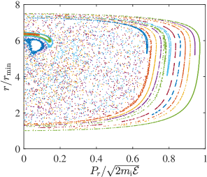
In the presence of non-paraxial regions, where , which seems to be typical for the diamagnetic bubble equilibrium (Kotelnikov et al., 2010; Kotelnikov, 2011; Beklemishev, 2016; Khristo & Beklemishev, 2019, 2022), the adiabaticity criterion (3) seems to be violated for the majority of the injected ions. In particular, Figure 1 illustrates an example of the ion Poincaré map in the central plane, , for various initial conditions and fixed energy and angular momentum . The magnetic field distribution is taken from the MHD simulations of the diamagnetic bubble equilibrium in GDMT (see Khristo & Beklemishev, 2022). Vacuum magnetic field in the central plane is , the ion Larmor radius in the vacuum magnetic field is and the minimum distance from the trap axis that the ion can approach is . It can be seen that a considerable region, corresponding to transverse momentum in the range , is filled with chaotic trajectories.
Strictly speaking, the ion dynamics should be considered separately for the chaotic and regular trajectories. In the chaotic region, the distribution function can be considered depending only on the integrals of motion: energy and angular momentum . At the same time, in the region of regular motion, these are also supplemented by the dependence on a third conserved quantity, for instance, the adiabatic invariant . On top of that, required is also a correct description of the transition region, separating chaotic and regular trajectories. This issue appears to be quite complex and needs to be addressed in an individual paper. For this reason, in the present article, we limit ourselves to considering the simplest case. Namely, we further assume that the region of the hot ion regular motion has a negligible measure, while the dynamics of the hot ions is globally chaotic and their trajectories ergodicly fill the hypersurfaces of constants and . Since the chaotic behavior appears to result from the collisionless scattering on the non-paraxial end regions: , we also assume that the characteristic ergodization time is on the order of several periods of longitudinal oscillations .
Hot ion distribution function
As noted above, we consider the hot ion density to be small enough to neglect their collisions with each other. In addition, we neglect the angular scattering of the hot ions in collisions with the warm plasma particles and take into account only the warm electron drag force
| (27) |
where is the hot ion velocity,
| (28) |
is the inverse ion slowing down time (Trubnikov, 1965), is the ion mass normalized to proton mass , is the ion-electron Coulomb logarithm. In what follows, we assume that the neutral beam is injected into the absolute confinement region (2); in this case, the loss of the hot ions can be ignored. Therefore, in the stationary case under consideration, the kinetic equation for the distribution function of the hot ions has the following invariant form:
| (29) |
where is the six-dimensional vector of generalized phase variables, is the corresponding phase velocity vector, is the nabla differential operator in the -space, and is the phase density of the hot ion source intensity, the explicit form of which is determined by the injection. Specifying the variables as , we obtain the equations of motion in the form:
Since we assume axial symmetry, the distribution function and the magnetic flux do not depend on the cyclic variable .
As mentioned above, we consider that the dynamics of ions is globally chaotic, and the ergodization time is on the order of several periods of longitudinal oscillations of the ion . Since the characteristic slowing down time significantly exceeds the characteristic bounce time (typically ), the drag force (27) can be considered weak on time scales of the period of longitudinal oscillations . By means of the conventionally used Krylov-Bogoliubov-Mitropolsky averaging approach (Bogoliubov & Mitropolskii, 1961), the slow phase space diffusion associated with the drag force (27) can be separated from the fast longitudinal oscillations. Based on this, we replace the exact kinetic equation (29) by an averaged one, assuming that the averaging should be performed over the surface in the phase space.
Instead of it is convenient to use the new variables , where is defined by
Hence, we have
and we should also keep in mind the additional condition , which defines the region of permissible values of the new variables. Then averaging of some quantity over the surface is performed as follows:
| (30) |
where
is the phase volume of the hypersurface . Finally, in the leading order with respect to , when the distribution function approximately depends only on and , averaging the perturbed system yields
| (31) | |||
Solving the kinetic equation (31) one can find the averaged distribution function of the hot ions . This in turn enables the density of some quantity to be obtained:
In particular, the azimuthal electric current density of the hot ions is given by
| (32) |
the power density of heating the warm plasma by the hot ions is defined as
| (33) |
6 Cylindrical bubble model
The complete system of equations describing the equilibrium of the diamagnetic bubble with neutral beam injection consists of the equation for the magnetic field (5) and the equations of material equilibrium (17) and thermal equilibrium (20) for the warm plasma. This system should be supplemented with the equation of state for the warm plasma (10) and the expression for the warm plasma current density (11), as well as the expressions for the hot ion current density (32) and heating power density (33). Finally, the formulation of the problem is completed by setting the boundary conditions for the magnetic field: (6), (7), and (8), the latter of which determines the boundary of the bubble core, and also the internal (23), (24), and external (25) conditions for the warm plasma equilibrium equations.
Just as it was done by Beklemishev (2016) for the case of MHD equilibrium, we further consider a simplified model of a cylindrical diamagnetic bubble. In the central part of such a bubble, there is a cylindrical core of length and radius with zero magnetic field: ; outside the core, for , the magnetic field lines are straight: . At the ends of the central cylindrical part, there are non-paraxial regions gradually turning into the mirror throats with the magnetic field . In addition, the source of the warm plasma is further considered to be entirely contained inside the bubble core. In this case, the density of the warm plasma inside the core is expected to be much higher than outside. Since the drag force (27) is proportional to the density of the warm plasma, the hot ions seem to slow down and release the energy mainly inside the bubble core as well.
6.1 Magnetic field distribution
The equilibrium equation for the magnetic field (5) can only be considered in the central cylindrical region, and the magnetic flux in the mirrors is considered to be given: . Then, after substituting the current density of the warm plasma (11), the equation (5) predictably reduces to the paraxial equilibrium with the Lorentz force from the hot ions:
| (34) | |||
| (35) |
In this equations we use the flux coordinate , so is the inverse function of and is essentially the radius of the magnetic surface that corresponds to the magnetic flux . In addition, the magnetic field and the current density of the hot ions should also be considered here as functions of . The corresponding boundary conditions (6), (7), and (8) can be reduced to
| (36) | |||
| (37) |
where is the vacuum magnetic field at the central section of the trap.
6.2 Warm plasma equilibrium
Warm plasma equilibrium equations (17) and (20) mainly remain the same except for the transport coefficients and , which are reduced to a simpler form in the cylindrical bubble approximation:
| (38) | |||
| (39) | |||
Here we also take into account that due to the hot ions mainly slowing down inside the bubble core, the external hot ion heating power release is negligible, i.e. and for . The boundary conditions (23), (24), and (25), in turn, remain exactly the same, except that and now have the meaning of the total absorbed injection power and the total warm plasma source, respectively.
6.3 Hot ion equilibrium
Consider the injection of a monoenergetic neutral beam with the injection energy and the total absorbed injection power . The injection is carried out at the angle to the axis of the trap, and the distance from the beam to the trap axis is finite and equal to . In this case, the source in the kinetic equation (31) has the form888In a real experiment, the beam has a finite width and angular spread, and it is also not exactly monoenergetic. Nevertheless, any injection can be represented as a combination of beams of type (40). In other words, the solution of the kinetic equation with such a right-hand side is essentially a Green’s function.:
| (40) |
where is the Dirac delta function,
| (41) |
is the angular momentum of the injected ions. Due to the beam slowing down mainly in the core of the bubble, averaging in (31) yields
where . The resulting kinetic equation
is satisfied by
| (42) |
where the phase volume is approximately equal to
and is the effective potential (26) in the central plane.
The remaining integral in can be represented in a simpler form. To do this, we further assume that, first, there is no reversed field and, second, the magnetic field either increases with the radius or decreases not faster than . In other words, the following conditions are met:
It can be shown that in this case, the effective potential has only one minimum. Consequently, the equation has no more than two roots: and , which are the radial boundaries of the integration domain . These roots are essentially the minimum and maximum distance from the axis available to a hot ion with energy and angular momentum . In what follows, and are shortly referred to as the minimum radius and the maximum radius, respectively, and we also define the corresponding minimum and maximum radii for the injected ions: and . Eventually, the phase volume can be represented in the following form:
It is worth noting that the minimum radius for the ions passing through the interior of the bubble core can be found explicitly. Indeed, since in the bubble core, for we have:
Note that the solution (42) also implies that in the approximation considered, the hot ion energy and angular momentum are related as follows: . This means that the minimum radius for the ions injected in the bubble core () remains constant:
Given (41), the minimum radius can also be expressed in terms of the injection radius and injection angle : . In addition, it follows that the sign of the angular momentum does not change during the ion slowing down, and the ions initially injected into the absolute confinement region (2) always stay in it:
Therefore, the axial loss of the hot ions can indeed be neglected999In fact, collisional angular scattering at low energies of course should eventually lead to the loss of the hot ions. The balance of the hot ions with the distribution (42) essentially assumes the presence of a sink in phase space at ..
Eventually, using the resulting distribution function (42) and the definition (32), we obtain the azimuthal diamagnetic current density of the hot ions:
| (43) |
where is the characteristic magnetic flux induced by the hot ion current, is the characteristic Larmor radius of injected ions, the coefficient
is the characteristic energy density of the hot ions, and
is the maximum radius of the hot ions with the distribution (42), which is to be found from the equation reduced to explicit form:
| (44) |
In particular, the outer boundary is .
7 Thin transition layer limit
The resulting complete system of equilibrium equations for a cylindrical bubble (34), (35), (38), and (39) accompanied by the expression for the hot ion current (43) proves to be essentially nonlinear. An exact equilibrium solution can only be obtained numerically. Detailed numerical simulations and analysis of the corresponding numerical equilibria are planned to be provided in future work. In the present paper, we focus on considering a limiting case that allows a significant simplification of the equations.
As mentioned at the beginning of Section 2, at the boundary of the diamagnetic bubble, right beyond the core, there is a transition layer inside which the magnetic field changes from to . The total thickness of this layer – the radial size of the region such that – is further denoted by . The inner boundary of the layer corresponds to the radial boundary of the bubble core, where the magnetic field is zero: . The outer boundary is the radius at which the diamagnetic current density of the plasma vanishes and the magnetic field reaches the vacuum value: . In other words, the outer boundary of the transition layer represents the boundary of the plasma. In the same way, we define separately the boundaries for the warm plasma and hot ion ions , beyond which the corresponding diamagnetic currents vanish; and are further naturally called the thicknesses of the transition layer for the warm plasma and the hot ions, respectively. It is clear that the total thickness of the transition layer is determined by the largest one: .
The transition layer thickness for the warm plasma is determined by the characteristic scale of the warm plasma resistive transverse diffusion across the magnetic field, which is normally quite small. In particular, the MHD equilibrium model (Beklemishev, 2016) shows that the thickness of the transition layer proves to be approximately equal to , where
| (45) |
is the characteristic thickness of magnetic field diffusion into the plasma and is the gas-dynamic lifetime. In the case of ’classical’ Spitzer conductivity , for the typical parameters: , , , the quantity is on the order of tenths of a centimeter. However, in the presence of the hot ion component, MHD is not applicable, and this estimate ceases to be valid.
For the distribution (42), the outer boundary, at which the current of the hot ions (43) vanishes, corresponds to the maximum radius of the injected ions . Then the thickness of the hot ion transition layer in this case is equal to . On the other hand, the hot ion transition layer is essentially the boundary region inside which the hot ions are ’reflected’ from the external vacuum magnetic field outside the bubble core, and its thickness seems to be proportional to the Larmor radius of the injected ions . Under typical conditions, the hot ion Larmor radius is on the order of centimeters and normally proves to be much greater than the warm plasma transverse diffusion scale . Thus, the total transition layer thickness could be expected mainly determined by the hot ion transition layer thickness: .
Further in this work, we consider the limit of the thin transition layer , which allows the model equations to be greatly simplified. Since normally decreases with increasing magnetic field, this approximation seems to correspond to the case of a sufficiently strong vacuum field .
7.1 Equilibrium magnetic field distribution
The magnetic field equilibrium is determined by the equations (34) and (35) with the boundary conditions (36) and (37). When solving these equations, we consider the pressure profile of the warm plasma given, implying that it can be found from the corresponding equilibrium equations (38) and (39). At the same time, the diamagnetic current of the hot ions is determined by the expression (43).
It is further convenient to use the following dimensionless quantities:
where is the warm plasma pressure normalized to the energy density of the vacuum magnetic field , also referred to simply as the relative pressure of the warm plasma. According to this, we also define the dimensionless minimum and maximum radii as follows:
where the latter is determined by the equation
| (46) |
which results from the corresponding normalization of the equation (44). Then the equations (34) and (35) with substituted hot ion current (43) take the following dimensionless form:
| (47) | |||
| (48) |
where
Normalizing the boundary conditions (36) and (37) yields:
| (49) | |||
| (50) |
As mentioned above, the hot ion transition layer thickness appears to be on the order of the Larmor radius of the injected ions , which means that in the thin transition layer limit before us , we should also expect the ratio to be small. Given this, it seems appropriate to apply the method of successive approximations by considering the coefficient in the right-hand side of the equation (48) as a small expansion parameter. Namely, we further assume that the solution of the system (47) and (48) can be represented in the form of an asymptotic expansion.
For a given magnetic field profile , by integrating the equation (48) and taking into account the boundary condition (49), the radius as a function of the magnetic flux can be explicitly expressed:
| (51) |
In the leading order of the approximation , when small corrections are completely neglected, the expression (51) reduces to
| (52) |
Substituting (52) into the equation (46) yields the corresponding approximation for the maximum radius:
| (53) |
The obtained formulas (52) and (46) correspond to . In other words, on the scale of the transition layer, the radius can be considered almost constant and equal to the bubble radius , while the magnetic flux varies greatly. At a qualitative level, this is associated with the high density of the diamagnetic current inside the layer.
Taking into account (52) and (53), the integral in the right-hand side of the equation (47) is evaluated explicitly:
As can be seen, the outer boundary of the hot ions in this order of approximation corresponds to . Given the boundary conditions (49) and (50), the resulting equation yields:
| (54) |
where
and is the relative pressure of the warm plasma inside the bubble core. In the absence of surface currents, the solution (54) should be continuous at the boundary , from which we also obtain the following condition:
| (55) |
Here, the quantity
can be interpreted as the characteristic relative energy density of the hot ions in the bubble. The formula (55) essentially expresses the balance between the plasma pressure inside the bubble and the pressure of the external magnetic field.
By applying the successive approximations to find higher orders of the expansion, the solution can be further refined. In particular, taking into account first order corrections in the expression (51) yields:
Using the obtained dependence, the corresponding correction to the maximum radius is also found from the equation (46):
For this formula determines the thickness of the hot ion transition layer:
| (56) |
Further in this paper, we consider the equilibrium configuration of the magnetic field to be approximately defined by (52) and (54) at . In other words, we take into account only the leading order of the asymptotic expansion. The applicability criterion for this approximation is determined by the limit
which is actually assumed in the derivation of (54). After substituting (56), we arrive at the following condition:
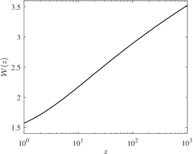
An upper bound for the integral involved can be obtained as follows:
where
| (57) |
As can be seen from Figure 2, for all reasonable the function is on the order of .
Before moving on to considering the equilibrium of the warm plasma, it is also useful to examine the expression (55) in greater detail. For given parameters of the warm plasma inside the bubble core: density and temperature , which are to be found from the solution of the equilibrium equations (38) and (39), the expression (55) defines the relation between the radius of the core and the fixed external parameters: absorbed heating power , vacuum magnetic field , and geometric parameters and . After expressing the warm plasma density from the equation of state (10), the formula (55) is reduced to a cubic equation for the normalized core radius :
| (58) |
where
Provided that the core radius exceeds the minimum radius , i.e. , this equation has exactly one real root for a fixed :
where and . This means that for a given temperature in the core , which we further consider determined by (67), this root specifies the functional dependency of the core radius on the pressure in the core: .
7.2 Warm plasma equilibrium
The equilibrium of the warm plasma is described by the equations (38) and (39) with the boundary conditions (23), (24) and (25). In what follows, the electrical and thermal conductivity of the warm plasma are considered classical (Braginskii, 1965):
| (59) | |||
In addition, the warm plasma flow velocity in the mirror is assumed to be
which correspond to the gas-dynamic loss in the case of short mirrors and a filled loss cone (Ivanov & Prikhodko, 2017). In what follows, we also consider , assuming the leading order of the thin transition layer approximation .
Let us show that in this case there exists an equilibrium of the warm plasma such that the temperature can be considered slowly varying on the scale of the warm plasma inhomogeneity:
| (60) |
Subtracting the equation (38) multiplied by from the equation (39) yields:
Taking into account the condition (60), the left-hand side of the resulting expression is approximately reduced to an exact differential:
which further allows the equation to be explicitly integrated. The constant of integration should be set equal to zero, since at the boundary of the warm plasma, where , the transverse fluxes of ions and energy should vanish. Finally, we find the slope factor:
| (61) |
For hydrogen plasma , and , which is typical for GDT (Ivanov & Prikhodko, 2017; Skovorodin, 2019; Soldatkina et al., 2020), the slope factor proves to be quite small: .
When the condition (60) is met, the equilibrium equations (38) and (39) are equivalent and reduced to:
| (62) |
where we use the dimensionless magnetic flux normalized to , and is defined by (45). We also introduce the quantity , which has the meaning of the warm plasma transverse flow. The magnetic field distribution is given by (54) taking into account the corresponding renormalization of the magnetic flux: , where corresponds to the boundary of the hot ions . When solving the equation (62), according to the approximation (60), the temperature should be considered constant and equal to . Further, a weak temperature dependence can be found from the equality (61):
| (63) |
Internal boundary conditions (23) and (24) also merge into one:
| (64) | |||
| (65) |
with an additional condition:
| (66) |
which defines the relationship between the temperature and the pressure of the warm plasma in the bubble core. For simplicity, we further assume , then the temperature of the warm plasma can be explicitly found from the equality (66). It proves to be independent of the pressure and is determined by the ratio of the sources:
| (67) |
External boundary conditions (25) are reduced to the following:
| (68) |
where corresponds to the outer boundary of the warm plasma . The second condition is essentially the vanishing of the transverse flow at the boundary, which is consistent with the pressure gradient and the current density being finite. It is also worth noting that the position of the boundary is not specified and should be found self-consistently from the solution of the equilibrium equation (62). This means that the two conditions (68) are related by and are formally reducible to one. In other words, one of the expressions (68) can be considered as a boundary condition, and the other as a definition of the boundary position .
7.3 Numerical solution
The boundary value problem (62), (64) and (66) described above turns out to be rather complex, and to find its exact solution we use numerical methods.
As mentioned above, provided that the temperature is given by the expression (67), the equation (58) relates the radius of the bubble core and the pressure of warm plasma in the core: . This means that remains the only free (i.e. unknown yet) parameter that determines the equilibrium. In that regard, the boundary value problem before us is convenient to reformulate as the following Cauchy problem. The equilibrium equations (62) can be considered as the system of ordinary differential equations for the functions and with the initial conditions (64) and . At the same time, the quantity should be treated as a variable parameter, which is found from the external boundary condition (68).
To solve the formulated problem, we apply an approach similar to the shooting method. For a given parameter , the equations (64) are integrated by means of the Runge-Kutta methods, starting from the corresponding initial conditions at . Computing continues until either or hits zero at some point 101010Here, we explicitly highlight the parametric dependence of the solutions and , as well as the warm plasma boundary position , on the parameter . . Thus, by varying the parameter , we can formally obtain the functional dependence . On the other hand, for a given relation , the conditions (68) are actually reduced to an equation for on the finite interval . The root of this equation, which can be found using standard numerical methods, is a true value of the parameter corresponding to the real equilibrium profile .
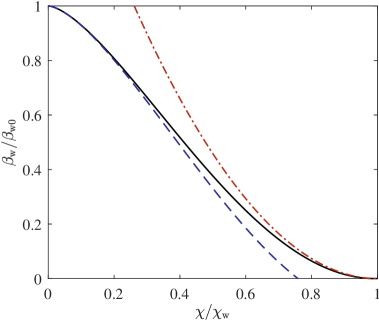
Figure 3 shows the numerical solution of the warm plasma equilibrium equation, found using the procedure described above. There are also plotted the corresponding analytical asymptotics in the vicinity of the bubble core and the outer boundary of the warm plasma, respectively:
| (69) |
| (70) |
where
The second term in the expansion (69) includes the contribution from the hot ions – it corresponds to the pressure profile of the warm plasma in the magnetic field induced by the hot ion current only. The third term, in turn, takes into account the diamagnetic current of the warm plasma. The non-polynomial logarithmic contribution of the hot ion current appears in the fourth term of the expansion.
8 Diamagnetic confinement in GDMT
As an application of the constructed theoretical model, we further investigate the equilibrium of the diamagnetic bubble corresponding to the design parameters of the GDMT device (Skovorodin et al., 2023). Hydrogen plasma is assumed: ; the axial loss constants correspond to GDT (Ivanov & Prikhodko, 2017; Skovorodin, 2019; Soldatkina et al., 2020): ; the Coulomb logarithm is set equal to . Energy, angle and impact parameter of the injection are , and , respectively, which corresponds to the minimum radius of the hot ions equal to . The bubble length is estimated from the MHD equilibrium simulations of GDMT (Khristo & Beklemishev, 2022) and is equal to . The total warm plasma source intensity is fixed at . The magnetic field in the mirrors is .
| Quantity | Units | Regime | ||
|---|---|---|---|---|
| GDMT05 | GDMT10 | GDMT20 | ||
| ∘ | ||||
| a) | ||||
| b) | ||||
We consider the conventional case of the vacuum magnetic field equal to , as well as the regimes with halved and doubled fields: and . In all the simulations, the radius of the bubble core is fixed at , which is the characteristic expected plasma radius in the GDMT. Then the required total absorbed injection powers prove to be , and for , and , respectively. For convenience, the simulation parameters are listed in Table 1, where the considered regimes are briefly called ’GDMT05’, ’GDMT10’ and ’GDMT20’.
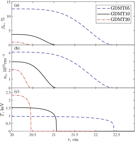
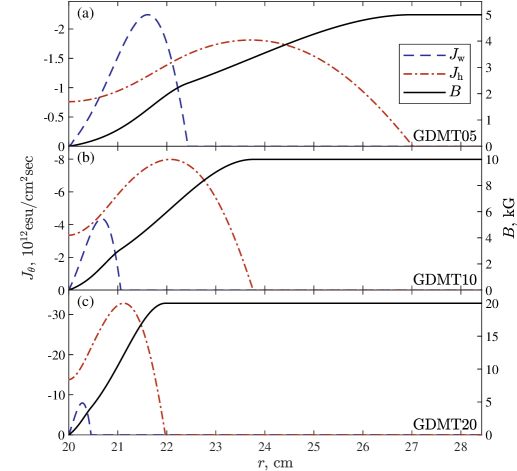
The results of the simulations are shown in Figures 4 and 5. Figure 4 shows the radial profiles of the warm plasma relative pressure, density and temperature outside111111Inside the bubble core , the warm plasma is isotropic, homogeneous and perfectly conducting, which corresponds to the magnetic field and the total diamagnetic plasma current being identically zero inside the core (see Section 4). the bubble core . The radial profiles of the magnetic field, along with the current densities of the warm plasma and the hot ions, outside the core are presented in Figure 5.
Analysis of the solutions
-
1.
For all solutions the relative energy density of the hot ions is significantly greater than the warm plasma relative pressure (see Table 1 and Figure 4):
(71) Thus, it turns out that the energy content of the plasma as well as the diamagnetic current almost entirely correspond to the hot ions, while the contribution of the warm plasma is negligible. Since the warm plasma density in this case should be relatively small, the drag force (27) acting on the injected ions appears to be weak as well. Therefore, this results in the energy being accumulated by the hot component rather than being transferred to the warm plasma, which is actually consistent with (71).
-
2.
In Table 1, listed are the simulated values of the transition layer thickness for the warm plasma and the hot ions , determined from the corresponding current profiles plotted in Figure 5. As expected, the total transition layer thickness is manly determined by the hot component, since the transition layer for the warm plasma proves to be much thinner than that for the hot ions . The thickness of the transition layer for the hot ions naturally turns out to be on the order of the Larmor radius of the injected ions in the vacuum magnetic field: . At the same time, the warm plasma transition layer thickness proves to be surprisingly close to the estimate made for MHD equilibrium (Beklemishev, 2016): . This effect is probably due to a combination of the following two factors. On the one hand, the warm plasma transition layer should apparently be wider in the presence of injected ions, since the characteristic scale of the warm plasma transverse diffusion proves to be greater in the magnetic field weakened by the diamagnetism of the hot component. On the other hand, for a fixed warm plasma source, the lower maximum relative pressure of the warm plasma (71) seems to correspond to a radial pressure drop in a more narrow region. A more clear explanation of this phenomenon and a proper quantitative estimate of the thickness should be made based on analysis the warm plasma equilibrium equations, which is planned to be addressed in future work.
-
3.
The equilibria presented in Figures 4 and 5 are obtained within the thin transition layer limit (see Section 7). For all the solutions found, the expansion parameter proves to be less than unity. However, in the regime GDMT05 with relatively weak vacuum magnetic field (Figure 5(a)), the expansion parameter is not too small: . A proper description of such equilibria should be obtained by accurate numerical modeling that takes into account the finite thickness of the transition layer.
-
4.
To simplify the system of the warm plasma equilibrium equations presented in Section 7.2, we assume the temperature of the warm plasma to be approximately constant: . As a result, the temperature profiles determined by the formula (63) actually prove to be relatively flat, but in addition, the corresponding pressure and density profiles turn out to be identically shaped (see Figure 4). It is worth noting, however, that the approximation of a slowly varying temperature is valid in the particular case of the hydrogen plasma with the energy loss factor corresponding to the GDT (Ivanov & Prikhodko, 2017; Skovorodin, 2019; Soldatkina et al., 2020), i.e. and . At the same time, the nature of energy loss in the diamagnetic confinement mode may differ significantly from the gas-dynamic regime. In particular, the presence of the non-adiabatic loss (Chernoshtanov, 2020, 2022) could greatly affect both longitudinal and transverse equilibrium.
-
5.
In Section 6.3, we assume that the injected hot ions release the energy mainly inside the bubble core. As already mentioned, the warm plasma temperature radial profile turns out to be almost flat, while the density of the warm plasma sharply drops just beyond the bubble core on the scale of (Figure 4). In the thin transition layer approximation , this results in the ion-electron drag indeed acting mainly inside the core. However, this appears to take place only when the source of the warm plasma is entirely contained inside the bubble core. Otherwise, the maximum density of the warm plasma could be located outside the core, which, apparently, could significantly increase the energy loss.
-
6.
The simulations also yield the parameter (see Table 1), which represents the total proportion of the non-adiabatic loss (22) in the total warm plasma loss. It can be seen that the warm plasma loss turns out to be almost entirely non-adiabatic for all the considered regimes:
(72) while the loss at the periphery of the bubble core proves to be negligible: . One can also observe that the parameter grows with increasing vacuum magnetic field. The reason for this is probably related to the high energy density of hot ions (71). The strong diamagnetism induced by the hot ions extending beyond the bubble core leads to a considerable weakening of the magnetic field in the vicinity of the bubble core . Therefore, the effective mirror ratio inside the thin transition layer is greatly increased compared to the vacuum value . This should eventually result in the axial loss at the periphery being suppressed due to a decrease in the cross section of the warm plasma flow in the mirrors . At the same time, the non-adiabatic loss , being determined by the vacuum mirror ratio , is not affected by the diamagnetism of the hot ions.
-
7.
The warm plasma density turns out to be considerably lower in the regimes with a higher temperature of the warm plasma (see Figure 4 and Table 1). This appears to be due to the improved confinement resulting from the suppression of the axial loss in the regimes with a lower warm plasma temperature. When the non-adiabatic loss dominates, the warm plasma density can be approximately estimated from (72):
(73) where
is the characteristic time of the non-adiabatic loss. It turns out that the efficiency of the axial confinement does not depend explicitly on the mirror ratio , as for a ’classical’ gas-dynamic trap , but it is enhanced with increasing the absolute value of the mirror magnetic field . In addition, the warm plasma density and the confinement time indeed prove to be greater at a lower warm plasma temperature . The inverse dependence of on is the result of the non-adiabatic loss (22) being proportional to .
-
8.
It can be observed from the simulations (see Figure 4 and Table 1) that the warm plasma temperature proves to be higher in the regimes with a stronger vacuum magnetic field . Indeed, sustaining the diamagnetic confinement equilibrium with stronger external field (at fixed mirror field , length and radius of the bubble core) requires greater absorbed injection power , while the increased heating power , in turn, should result in a corresponding rise in the equilibrium temperature of the warm plasma . This relation can be clarified by considering the force balance in the case of beam plasma (71):
where
are the characteristic energy densities of the hot ions and the vacuum magnetic field, respectively. This expression roughly corresponds to the equation (58) in the limit: , and . Taking into account the estimate (73), we obtain the following relation:
(74) Therefore, the temperature of warm plasma indeed proves to increase with the vacuum magnetic field as .
-
9.
Having fixed the mirror field , the warm plasma source , the radius and the length of the bubble core, from the considered above qualitative estimates (73) and (73), we get
Given the error due to the corresponding inaccuracy of the estimate (72), these relations agree well with the results of the simulations shown in Figure 4 and Table 1.
-
10.
In the present paper, we assume the classical model of transverse transport for the warm plasma, which corresponds to the Spitzer conductivity (59). At the same time, large gradients of equilibrium parameters, such as the magnetic field and the warm plasma density, inside the transition layer of the diamagnetic bubble could probably lead to non-classical transport, which corresponds to a much greater diffusion coefficient. In turn, a significant modification of the transverse transport could apparently have a qualitative impact on the equilibrium of the warm plasma. However, the issue concerning non-classical diffusion in the diamagnetic confinement mode remains poorly studied so far.
-
11.
The model of the warm plasma equilibrium, constructed in Section 4 within the framework of MHD, assumes isotropic pressure and gas-dynamic axial loss. This is known to correspond to the collisional regime with a filled loss cone. In the case of GDT (Ivanov & Prikhodko, 2017), such a regime is realized when the gas-dynamic time significantly exceeds the kinetic time , where is the mean free time of ion-ion Coulomb collisions (Trubnikov, 1965). However, when considering a diamagnetic trap, one should also take into account the effective increase in the mirror ratio , which results from the magnetic field weakening induced by the strong diamagnetic current of the high-pressure plasma. In addition, the exotic conditions of the diamagnetic confinement mode are likely to lead to anomalous collisionality with an effective mean free time , which typically proves to be considerably shorter than the ’classical’ time . Thus, the warm plasma loss cone in the transition layer of a diamagnetic bubble can be considered filled when
This condition seems to be always satisfied at least in some neighborhood of the bubble core , where the magnetic field approaches zero , and, accordingly, the effective mirror ratio is greatly increased . At the periphery of the warm plasma , the loss cone may turn out to be only partially filled () or even empty (), depending on the specific value of the anomalous mean free time .
9 Summary
In the present work, we have constructed the theoretical model of plasma equilibrium in the diamagnetic confinement regime in an axisymmetric mirror device with neutral beam injection. To describe the equilibrium of the background warm plasma, we use the MHD equations of mass and energy conservation, as well as the force balance equation. Transverse transport is considered to be due to resistive diffusion, and the axial loss includes both the ’classical’ gas-dynamic loss and the non-adiabatic loss (Chernoshtanov, 2020, 2022) specific to the diamagnetic bubble. This model does not take into account the effects of the warm plasma rotation and inhomogeneity of electrostatic potential. The equilibrium of the hot ions resulted from the neutral beam injection is described by the distribution function, which is found from the corresponding kinetic equation. It takes into account the warm electron drag force acting on the hot ions, while the angular scattering due to the ion-ion collisions is neglected. The chaotic nature of the dynamics of ions in the diamagnetic bubble is taken into consideration as well. Solving the equilibrium equations yields the equilibrium profiles of the warm plasma density, temperature and pressure; the hot ion current density is obtained from the corresponding distribution function; the equilibrium magnetic field is determined by Maxwell’s equations.
Applying the constructed theoretical model, we have considered the case of the cylindrical core of the diamagnetic bubble. In this case, the equilibrium model is reduced to a simpler one-dimensional problem. To further simplify the equations, we have assumed the approximation of the thin transition layer. This allows the hot ion current density and the magnetic field to be explicitly expressed in terms of the magnetic flux. Finally, it has been found that the radial profile of the warm plasma typically turns out to be almost isothermal, which enables the system of two equilibrium equations for the warm plasma to be approximately reduced to a single one. For the resulting equation of the simplified equilibrium model, we have constructed a numerical solution algorithm that includes a variation of the shooting method in combination with the Runge-Kutta schemes.
The equilibria of the diamagnetic bubble have been found for the parameters of the GDMT device (Skovorodin et al., 2023). Three cases corresponding to different vacuum magnetic fields in the central plane, , have been considered. All the other external parameters are fixed except the absorbed injection power, which is adjusted so that the radius of the bubble core remains the same . Equilibrium profiles of the warm plasma density, temperature and pressure have been found. In addition, the radial distributions of the magnetic field and the diamagnetic current densities of the warm plasma and the hot ions have been constructed.
It has been found that for all the solutions obtained, the main contribution to the plasma energy content and the diamagnetism comes from the hot ions. This corresponds to a negligible relative pressure of the warm plasma . In addition, the non-adiabatic loss turns out to be dominant in all considered regimes, and its fraction in total loss is greater for stronger vacuum magnetic field. This seems to be due to the warm plasma in the transition layer being confined in the magnetic field weakened by the hot ion diamagnetism, which should lead to an increased mirror ratio and improved axial confinement. The transition layer of the diamagnetic bubble turns out to be quite thin in the regimes with the stronger vacuum fields, . However, in the case of the weak external field, , the thickness of the transition layer proves to be not too small, which may correspond to a reduced accuracy of the approximate solution. Qualitative estimates of the warm plasma density and the temperature of the warm plasma have also been obtained.
Future work
This work should be considered as a basis for further expansion of the theoretical model constructed here. In the near future, the equilibrium model presented in this paper will be used for a detailed investigation of the diamagnetic confinement regime in GDMT. In particular, it is planned to study the dependence of the bubble equilibrium on external conditions, such as heating power, vacuum magnetic configuration, warm plasma source, etc. In addition, the finite absorption efficiency of the injected neutral beam can be taken into account. The constructed model can also be refined by eliminating the thin transition layer approximation; this, however, would require more complex numerical simulations. In perspective, it is also planned to include in the model the effects of the warm plasma rotation and the inhomogeneity of the electrostatic potential. In the long term, collisional angular scattering of the hot ions can also be taken into account.
10 Acknowledgments
The authors would like to express their gratitude to Vadim Prikhodko, Ivan Chernoshtanov, Dmitriy Skovorodin, Elena Soldatkina, Timur Akhmetov, Sergei Konstantinov and other colleagues from the plasma department of the Budker INP for helpful suggestions and productive discussions.
The work was supported by the Foundation for the Advancement of Theoretical Physics and Mathematics ’BASIS’.
Appendix A Non-adiabatic loss
By definition, the ion flux through the mirror throat at is
where is directed along the magnetic field in the mirror throat, and we also substituted the warm ion distribution function (21). Taking into account the definitions of and given by (1), we arrive at
where
is the magnetic flux in the mirror. It is convenient to further use the following dimensionless variables:
Then the integral takes the form:
where we introduced the constant
and is the warm ion thermal velocity, is the characteristic warm ion Larmor radius in the vacuum field , is the vacuum mirror ratio.
Integration over , , and is convenient to rearrange as follows:
where
and . Integrating over yields:
After integration over we get:
In the limit the second term in the square brackets proves to be exponentially small. Then we obtain the asymptotic behavior of the integral :
Restoring the dimensional values, we finally arrive at:
References
- Bagryansky et al. (2016) Bagryansky, P A, Akhmetov, T D, Chernoshtanov, I S, Deichuli, P P, Ivanov, A A, Lizunov, A A, Maximov, V V, Mishagin, V V, Murakhtin, S V, Pinzhenin, E I, Pikhodko, V V, Sorokin, A V & Oreshonok, V V 2016 Status of the experiment on magnetic field reversal at BINP. In AIP Conference Proceedings, , vol. 1771, p. 030015.
- Bagryansky et al. (2011) Bagryansky, P A, Anikeev, A V, Beklemishev, A D, Donin, A S, Ivanov, A A, Korzhavina, M S, Kovalenko, Yu V, Kruglyakov, E P, Lizunov, A A, Maximov, V V, Murakhtin, S V, Prikhodko, V V, Pinzhenin, E I, Pushkareva, A N, Savkin, V Ya & Zaytsev, K V 2011 Confinement of Hot Ion Plasma with = 0.6 in the Gas Dynamic Trap. Fusion Science and Technology 59 (1T), 31–35.
- Bagryansky et al. (2019) Bagryansky, P A, Beklemishev, A D & Postupaev, V V 2019 Encouraging Results and New Ideas for Fusion in Linear Traps. Journal of Fusion Energy 38 (1), 162–181.
- Beklemishev et al. (2013) Beklemishev, A, Anikeev, A, Astrelin, V, Bagryansky, P, Burdakov, A, Davydenko, V, Gavrilenko, D, Ivanov, A, Ivanov, I, Ivantsivsky, M, Kandaurov, I, Polosatkin, S, Postupaev, V, Sinitsky, S, Shoshin, A, Timofeev, I & Tsidulko, Yu 2013 Novosibirsk Project of Gas-Dynamic Multiple-Mirror Trap. Fusion Science and Technology 63 (1T), 46–51.
- Beklemishev (2016) Beklemishev, A D 2016 Diamagnetic “bubble” equilibria in linear traps. Physics of Plasmas 23 (8), 082506.
- Beklemishev et al. (2010) Beklemishev, Alexei D, Bagryansky, Peter A, Chaschin, Maxim S & Soldatkina, Elena I 2010 Vortex Confinement of Plasmas in Symmetric Mirror Traps. Fusion Science and Technology 57 (4), 351–360.
- Belchenko et al. (2018) Belchenko, Yu I, Davydenko, V I, Deichuli, P P, Emelev, I S, Ivanov, A A, Kolmogorov, V V, Konstantinov, S G, Krasnov, A A, Popov, S S, Sanin, A L, Sorokin, A V, Stupishin, N V, Shikhovtsev, I V, Kolmogorov, A V, Atlukhanov, M G, Abdrashitov, G F, Dranichnikov, A N, Kapitonov, V A & Kondakov, A A 2018 Studies of ion and neutral beam physics and technology at the Budker Institute of Nuclear Physics, SB RAS. Physics-Uspekhi 61 (6), 531–581.
- Berk et al. (1987) Berk, H L, Wong, H V & Tsang, K T 1987 Theory of hot particle stability. Physics of Fluids 30 (9), 2681–2693.
- Bogoliubov & Mitropolskii (1961) Bogoliubov, N N & Mitropolskii, Y A 1961 Asymptotic methods in the theory of non-linear oscillations. Gordon and Breach.
- Boronina et al. (2020) Boronina, M A, Dudnikova, G I, Efimova, A A, Genrikh, E A, Vshivkov, V A & Chernoshtanov, I S 2020 Numerical study of diamagnetic regime in open magnetic trap. Journal of Physics: Conference Series 1640 (1), 012021.
- Braginskii (1965) Braginskii, S I 1965 Transport Processes in a Plasma. In Reviews of Plasma Physics (ed. M A Leontovich), , vol. 1, p. 205. New York: Consultants Bureau.
- Chernoshtanov (2020) Chernoshtanov, Ivan 2020 Collisionless particle dynamic in an axi-symmetric diamagnetic trap, arXiv: 2002.03535.
- Chernoshtanov et al. (2023) Chernoshtanov, I, Efimova, A, Soloviev, A & Vshivkov, V 2023 Fast Ion–Ion Collisions Simulation in Particle-in-Cell Method. Lobachevskii Journal of Mathematics 44 (1), 26–32.
- Chernoshtanov (2022) Chernoshtanov, I S 2022 Collisionless Particle Dynamics in Diamagnetic Trap. Plasma Physics Reports 48 (2), 79–90.
- Chernoshtanov et al. (2024) Chernoshtanov, I S, Chernykh, I G, Dudnikova, G I, Boronina, M A, Liseykina, T V & Vshivkov, V A 2024 Effects observed in numerical simulation of high-beta plasma with hot ions in an axisymmetric mirror machine. Journal of Plasma Physics 90 (2), 905900211.
- Dimov (2005) Dimov, Gennadii I 2005 The ambipolar trap. Physics-Uspekhi 48 (11), 1129–1149.
- Efimova et al. (2020) Efimova, A. A., Dudnikova, G. I. & Vshivkov, K. V. 2020 3D numerical model of diamagnetic plasma confinement in gasdynamic trap. AIP Conference Proceedings 2312 (1), 060001.
- Grad (1967) Grad, Harold 1967 The guiding center plasma. In Proc. of Symposia in Applied Mathematics (ed. Harold Grad), Magneto-Fluid and Plasma Dynamics, vol. 18, pp. 162–248. Providence, Rhode Island: American Mathematical Society.
- Grad & Rubin (1958) Grad, H & Rubin, H 1958 Hydromagnetic equilibria and force-free fields. In Proc. of the Second UN International Conference on the Peaceful Uses of Atomic Energy, Theoretical and Experimental Aspects of Controlled Nuclear Fusion, vol. 31, pp. 190–197. Geneva, Switzerland.
- Hsiao & Miley (1985) Hsiao, Ming-Yuan & Miley, George H 1985 Velocity-space particle loss in field-reversed configurations. Physics of Fluids 28 (5), 1440.
- Ioffe et al. (1981) Ioffe, M S, Kanaev, B I, Pastukhov, V P, Piterskii, V V & Yushmanov, E E 1981 Plasma heating in a magnetic cusp confinement system without injection. Soviet Journal of Experimental and Theoretical Physics Letters 34 (11), 570–573.
- Ivanov & Prikhodko (2017) Ivanov, A A & Prikhodko, V V 2017 Gas dynamic trap: experimental results and future prospects. Physics-Uspekhi 60 (5), 509–533.
- Kaiser & Pearlstein (1985) Kaiser, T B & Pearlstein, L Donald 1985 Finite Larmor radius and wall effects on the M=1 ballooning mode at arbitrary beta in axisymmetric tandem mirrors. Physics of Fluids 28 (3), 1003–1005.
- Kaufmann et al. (1970) Kaufmann, Richard L, Horng, Jiann-Tsorng & Wolfe, Allan 1970 Large-amplitude hydromagnetic waves in the inner magnetosheath. Journal of Geophysical Research 75 (25), 4666–4676.
- Khristo & Beklemishev (2019) Khristo, Mikhail S & Beklemishev, Alexey D 2019 High-Pressure Limit of Equilibrium in Axisymmetric Open Traps. Plasma and Fusion Research 14, 2403007–2403007.
- Khristo & Beklemishev (2022) Khristo, M S & Beklemishev, A D 2022 Two-dimensional MHD equilibria of diamagnetic bubble in gas-dynamic trap. Plasma Physics and Controlled Fusion 64 (9), 095019.
- Kotelnikov (2020) Kotelnikov, Igor 2020 On the structure of the boundary layer in a Beklemishev diamagnetic bubble. Plasma Physics and Controlled Fusion 62 (7), 075002.
- Kotelnikov et al. (2022) Kotelnikov, Igor, Zeng, Qiusun, Prikhodko, Vadim, Yakovlev, Dmitri, Zhang, Keqing, Chen, Zhibin & Yu, Jie 2022 Wall stabilization of the rigid ballooning m = 1 mode in a long-thin mirror trap. Nuclear Fusion 62 (9), 096025.
- Kotelnikov (2011) Kotelnikov, I A 2011 Equilibrium of a High- Plasma with Sloshing Ions above the Mirror Instability Threshold. Fusion Science and Technology 59 (1T), 47–50.
- Kotelnikov et al. (2010) Kotelnikov, I A, Bagryansky, P A & Prikhodko, V V 2010 Formation of a magnetic hole above the mirror-instability threshold in a plasma with sloshing ions. Physical Review E 81 (6), 067402.
- Kurshakov & Timofeev (2023) Kurshakov, V A & Timofeev, I V 2023 The role of electron current in high- plasma equilibria. Physics of Plasmas 30 (9).
- Kuznetsov et al. (2015) Kuznetsov, E A, Passot, T, Ruban, V P & Sulem, P L 2015 Variational approach for static mirror structures. Physics of Plasmas 22 (4), 042114.
- Landsman et al. (2004) Landsman, A S, Cohen, S A & Glasser, A H 2004 Regular and stochastic orbits of ions in a highly prolate field-reversed configuration. Physics of Plasmas 11 (3), 947–957.
- Lansky (1993) Lansky, I M 1993 On the paraxial equilibrium of the finite plasma in open magnetic configuration. Tech. Rep. 93-96. Budker INP.
- Larrabee et al. (1979) Larrabee, D A, Lovelace, R V & Fleischmann, H H 1979 Truncated exponential-rigid-rotor model for strong electron and ion rings. Nuclear Fusion 19 (4), 499–503.
- Lichtenberg & Lieberman (1992) Lichtenberg, A J & Lieberman, M A 1992 Regular and Chaotic Dynamics, Applied Mathematical Sciences, vol. 38. New York, NY: Springer New York.
- Lotov (1996) Lotov, K V 1996 Spontaneous formation of zero magnetic field region near the axis of a high- mirror device. Physics of Plasmas 3 (4), 1472–1473.
- Lovelace et al. (1978) Lovelace, R V, Larrabee, D A & Fleischmann, H H 1978 A re-analysis of exponential rigid-rotor astron equilibria. Physics of Fluids 21 (5), 863.
- Morozov & Solov’ev (1966) Morozov, A I & Solov’ev, L S 1966 Motion of Charged Particles in Electromagnetic Fields. In Reviews of Plasma Physics (ed. M A Leontovich), , vol. 2, pp. 201–297. New York: Consultants Bureau.
- Newcomb (1981) Newcomb, William A 1981 Equilibrium and stability of collisionless systems in the paraxial limit. Journal of Plasma Physics 26 (3), 529–584.
- Pastukhov (1978) Pastukhov, V P 1978 Classical transport in electrostatically plugged magnetic confinement systems. Soviet Journal of Plasma Physics 4 (3), 311–316.
- Pastukhov (1980) Pastukhov, V P 1980 Anomalous electron transport in the transition layer of an electrostatically plugged magnetic mirror. Soviet Journal of Plasma Physics 6 (5), 549–554.
- Pastukhov (2021) Pastukhov, V P 2021 Turbulent Relaxation and Anomalous Plasma Transport. Plasma Physics Reports 47 (9), 892–906.
- Qerushi & Rostoker (2002a) Qerushi, Artan & Rostoker, Norman 2002a Equilibrium of field reversed configurations with rotation. II. One space dimension and many ion species. Physics of Plasmas 9 (7), 3068–3074.
- Qerushi & Rostoker (2002b) Qerushi, Artan & Rostoker, Norman 2002b Equilibrium of field reversed configurations with rotation. III. Two space dimensions and one type of ion. Physics of Plasmas 9 (12), 5001–5017.
- Qerushi & Rostoker (2003) Qerushi, Artan & Rostoker, Norman 2003 Equilibrium of field reversed configurations with rotation. IV. Two space dimensions and many ion species. Physics of Plasmas 10 (3), 737–752.
- Rostoker & Qerushi (2002) Rostoker, Norman & Qerushi, Artan 2002 Equilibrium of field reversed configurations with rotation. I. One space dimension and one type of ion. Physics of Plasmas 9 (7), 3057–3067.
- Ryutov (2005) Ryutov, D D 2005 Axial Electron Heat Loss from Mirror Devices Revisited. Fusion Science and Technology 47 (1T), 148–154.
- Sagdeev et al. (1988) Sagdeev, R Z, Usikov, D A & Zaslavsky, G M 1988 Nonlinear Physics: From the Pendulum to Turbulence and Chaos. Contemporary concepts in physics . Harwood Academic Publishers.
- Shafranov (1958) Shafranov, V D 1958 On Magnetohydrodynamical Equilibrium Configurations. Journal of Experimental and Theoretical Physics 6 (3), 545–554.
- Skovorodin (2019) Skovorodin, D I 2019 Suppression of secondary emission of electrons from end plate in expander of open trap. Physics of Plasmas 26 (1), 012503.
- Skovorodin et al. (2023) Skovorodin, D I, Chernoshtanov, I S, Amirov, V Kh, Astrelin, V T, Bagryanskii, P A, Beklemishev, A D, Burdakov, A V, Gorbovskii, A I, Kotel’nikov, I A, Magommedov, E M, Polosatkin, S V, Postupaev, V V, Prikhod’ko, V V, Savkin, V Ya, Soldatkina, E I, Solomakhin, A L, Sorokin, A V, Sudnikov, A V, Khristo, M S, Shiyankov, S V, Yakovlev, D V & Shcherbakov, V I 2023 Gas-Dynamic Multiple-Mirror Trap GDMT. Plasma Physics Reports 49 (9), 1039–1086.
- Soldatkina et al. (2008) Soldatkina, E I, Bagryansky, P A & Solomakhin, A L 2008 Influence of the radial profile of the electric potential on the confinement of a high- two-component plasma in a gas-dynamic trap. Plasma Physics Reports 34 (4), 259–264.
- Soldatkina et al. (2023) Soldatkina, Elena Ivanovna, Chernoshtanov, Ivan Sergeevich, Iakovlev, Dmitrii Vadimovich, Beklemishev, Aleksei Dmitrievich & Khristo, Mikhail Sergeevich 2023 Method for confining high-temperature plasma in open magnetic trap.
- Soldatkina et al. (2020) Soldatkina, E I, Maximov, V V, Prikhodko, V V, Savkin, V Ya, Skovorodin, D I, Yakovlev, D V & Bagryansky, P A 2020 Measurements of axial energy loss from magnetic mirror trap. Nuclear Fusion 60 (8), 086009.
- Steinhauer (2011a) Steinhauer, Loren C 2011a Hybrid equilibria of field-reversed configurations. Physics of Plasmas 18 (11), 112509.
- Steinhauer (2011b) Steinhauer, Loren C 2011b Review of field-reversed configurations. Physics of Plasmas 18 (7), 070501.
- Trubnikov (1965) Trubnikov, B A 1965 Particle Interactions in a Fully Ionized Plasma. In Reviews of Plasma Physics (ed. M A Leontovich), , vol. 1, p. 105. New York: Consultants Bureau.
- Tsurutani et al. (2011) Tsurutani, Bruce T, Lakhina, Gurbax S, Verkhoglyadova, Olga P, Echer, Ezequiel, Guarnieri, Fernando L, Narita, Yasuhito & Constantinescu, Dragos O 2011 Magnetosheath and heliosheath mirror mode structures, interplanetary magnetic decreases, and linear magnetic decreases: Differences and distinguishing features. Journal of Geophysical Research: Space Physics 116 (A2), A02103.
- Turner et al. (1977) Turner, J M, Burlaga, L F, Ness, N F & Lemaire, J F 1977 Magnetic holes in the solar wind. Journal of Geophysical Research 82 (13), 1921–1924.
- Zhitlukhin et al. (1984) Zhitlukhin, A M, Safronov, V M, Sidnev, V V & Skvortsov, Yu V 1984 Confinement of a hot plasma with 1 in an open confinement system. JETP Lett 39 (6), 293–296.