Majorana Collaboration
An assay-based background projection for the Majorana Demonstrator using Monte Carlo Uncertainty Propagation
Abstract
The background index is an important quantity which is used in projecting and calculating the half-life sensitivity of neutrinoless double-beta decay () experiments. A novel analysis framework is presented to calculate the background index using the specific activities, masses and simulated efficiencies of an experiment’s components as distributions. This Bayesian framework includes a unified approach to combine specific activities from assay. Monte Carlo uncertainty propagation is used to build a background index distribution from the specific activity, mass and efficiency distributions. This analysis method is applied to the Majorana Demonstrator, which deployed arrays of high-purity Ge detectors enriched in 76Ge to search for . The framework projects a mean background index of from 232Th and 238U in the Demonstrator’s components.
pacs:
23.40-s, 23.40.Bw, 14.60.Pq, 27.50.+jI Introduction
A variety of low background experiments form the rich experimental program searching for neutrinoless double-beta decay (). While the decay remains unobserved in all candidate isotopes, the half-life has been constrained to be above years by recent experiments [1, 2, 3, 4, 5]. The next generation of proposed experiments target a half-life sensitivity, , of years [6, 7, 8]. To achieve these sensitivities, experiments require underground locations, large isotopic mass and low-background construction materials. Extensive assay screenings are conducted to determine if the experiments structural components meet the targeted background levels.
In terms of the total electron kinetic energy, the experimental signature of is a peak at the Q-value of the decay, . If no background is present in this region of interest (ROI), the sensitivity of a experiment scales linearly with the product of its isotopic mass, , and exposure time, [9]. However, if the specific background rate, , is large enough (such that the uncertainty on the background level is proportional to [10]) the half-life sensitivity () scales with:
| (1) |
The width of the ROI, , is related to and the energy resolution at . The specific background rate is measured in counts per keV in the ROI, per kg of detector mass, per year (cts/(keV kg yr)). This observable is also referred to as the background index (BI). Given the low-background nature of experiments, the number of background counts in the ROI is typically too low to estimate the BI (note that no signal would have to be assumed). In such cases, a wider proxy region is needed to increase statistics. This background estimation window (BEW) is often asymmetric around to avoid running into the spectrum and known gamma lines.
Germanium detector technology has been developed for decades, finding applications in radiometric assays and -ray spectroscopy. Ge detectors offer superb energy resolution – resulting in a narrower ROI – and can be readily enriched to % 76Ge [11]. The Majorana Demonstrator and GERDA experiments exploited this technology to search for in 76Ge-enriched high purity Ge (HPGe) detectors [12]. Both experiments have the lowest backgrounds of any experiment in the present experimental landscape [2, 1].
At the 2039 keV Q-value of 76Ge [13, 14], the Demonstrator achieved a BI of cts/(keV kg yr) in its low background configuration [1]. This is not in agreement with the originally projected BI of cts/(keV kg yr) [15]. The projection was based on simulations of the design geometry and the results of an extensive radioassay program. To account for any discrepancies between the design and as-built geometries of the Demonstrator, a new set of simulations was performed with the updated geometries. This as-built model did not find a significant deviation from the originally predicted BI. Nevertheless, neither calculation captured the often significant uncertainties from assay in the contribution of natural radiation (BI) to the total BI. Additionally, a systematic review of assay results highlighted the prevalence of measured values that did not agree within error, motivating the development of a technique which properly accounts for this spread and propagates it into the BI.
The total BI includes subdominant contributions from, amongst others, external and cosmogenically induced backgrounds. For this work, only backgrounds quantified by assay – 232Th, 238U – are considered. While the components in the Demonstrator are also screened for 40K, it is excluded from the analysis since the -rays produced in the 40K decay chain have energies well below the BEW.
The BI is calculated by weighting the activity of a component with the Demonstrator’s simulated array-detection efficiency of decays originating from it. An upper limit on the activity of a component translates into an upper limit on its BI. In the previous projections, such upper limits were directly summed to BIs calculated from measured activities when summing over all modeled components of the Demonstrator. Thus, the total projected BI was reported as an upper limit itself. Null efficiencies were computed for some components far away from the detector array and failed to contribute to the BI. However, given the high activity of some of these components, their true contribution could still be significant. Therefore, simulation statistics must be properly taken into account.
Other experiments use techniques which address these issues in part. By repeatedly drawing samples from an activity probability density function (PDF) and weighting them by the simulated efficiency, a BI distribution is generated. The CUORE Collaboration generates activity PDFs from fits to preliminary data [16]. On the other hand, the nEXO Collaboration promotes assay-based activities to a truncated-at-zero Gaussian PDF [17]. The latter technique is adopted by this work and expanded on by promoting the single-valued efficiency to a distribution as well. Ref. [18] provides a comprehensive summary of the methods used to estimate the BI of various experiments.
In this article, an assay-based Bayesian framework to project the BI of low-background experiments is presented and applied to the Majorana Demonstrator. The framework takes as input all the assay and simulation efficiency data with the goal of:
-
1.
Combining multiple assay measurements, including upper limits, using a unified averaging method which properly accounts for the spread in data.
-
2.
Calculating uncertainties in non-Gaussian regimes such as those posed by null simulation efficiencies.
-
3.
Combining uncertainties in assay results, component masses and simulation statistics.
-
4.
Preserving the generality of this method, allowing for its adoption by the low-background community.
II The Majorana Demonstrator
The Majorana Demonstrator consisted of two modules (M1, M2) [19] where a total of 40.4 kg of HPGe detectors (27.2 kg enriched to 88% in 76Ge) operated in vacuum at the 4850-foot-level (4300 meter water equivalent) of the Sanford Underground Research Facility (SURF) [20] in Lead, South Dakota. The ultra-low background and world-leading energy resolution achieved by the Demonstrator enabled a sensitive decay search, as well as additional searches for physics beyond the Standard Model.
Both vacuum cryostats and all structural components of the detector arrays were machined from ultra-low-background underground electroformed copper (UGEFCu) [21, 15] and low-background plastics, such as DuPontTM Vespel® and polytetrafluoroethylene (PTFE). Low-radioactivity parylene was used to coat UGEFCu threads to prevent galling and for the cryostat seal [19]. A layered shield enclosed both modules. The innermost layer consisted of 5 cm of UGEFCu. Five cm of commercial oxygen-free high conductivity copper (OFHCCu) and 45 cm of high-purity lead followed. The shield and module volume were constantly purged with low-radon liquid nitrogen boil-off gas. The aluminum enclosure that isolated this Rn-excluded region was covered with a plastic active muon veto which provided near- coverage [22]. The near-detector readout system, which was designed for the Demonstrator, included low-mass front end (LMFE) electronics [23] and low-mass cables and connectors [24]. Cables were guided out of each module following a UGEFCu cross-arm which penetrated the layered shield. The cross-arm connected the cryostat with vacuum and cryogenic hardware. Control and readout electronics were just outside the Rn-excluded region. The entire assembly was surrounded by 5 cm of borated polyethylene and 25 cm of pure polyethylene to shield against neutrons.
All components inside the Rn-excluded region populate the as-built model. These were modeled in MaGe, the Geant4-based simulation software jointly developed by the GERDA and Majorana collaborations [25]. Due to possible radioactive shine through the cross-arm, the vacuum hardware was included as well. The as-built model is based on the Aug. 2016 to Nov. 2019 configuration of the Demonstrator, where up to 32.1 kg of detectors were operational. In Nov. 2019, M2 was upgraded with an improved set of cables and connectors and additional cross-arm shielding. The upgrade, in combination with a reconfiguration of M2 detectors, resulted in the final configuration of up to 40.4 kg of operational HPGe detectors. The final active enriched exposure of the Demonstrator was 64.5 kg yr. A low-background dataset – with an active exposure of 63.3 kg yr – was obtained by excluding data taken previous to the installation of the inner UGEFCu shield. From this dataset, a BI of cts/(keV kg yr) was calculated [1]. The previous data release of the Demonstrator does not include post-M2-upgrade data. The low-background dataset BI in this release is cts/(keV kg yr) with 21.3 kg yr of active exposure [26].
To simulate 232Th and 238U decays originating from the hardware components of the Demonstrator, their respective decay chains were divided into 10 and 4 segments respectively, following the prescription in Ref. [27]. Within each segment secular equilibrium was assumed. The breakpoints in the chains – which generally correspond to isotopes with half-lives longer than 3 days – allow a break in secular equilibrium. However, given that the concentration of these isotopes is unknown, secular equilibrium of the chain as a whole was assumed as well. For a particular component and decay chain, the same number of decays were simulated for each segment and the energy depositions in the detectors were recorded. These were later combined with the appropriate branching ratios to produce a spectrum. Section IV describes how the component efficiency is extracted from this simulated spectrum.
III A unified approach to combine assay results
The Demonstrator’s radioassay program delivered an extensive specific activity database (232Th, 238U, 40K) of the materials used to build the experiment [15]. During the commissioning of the Demonstrator, additional samples were collected and assayed, thus continually growing this database. Amongst others, inductively coupled plasma mass spectrometry (ICPMS), -count and neutron activation analysis (NAA) measurements were performed. The most sensitive technique, ICPMS, measures specific elements within a decay chain and therefore secular equilibrium is assumed to project a specific activity. The concentration of 232Th and 238U in HPGe detectors is far too low to be detected by ICPMS measurements. Thus, the 232Th and 238U contaminations are deduced by searching for time-correlated decays from their respective decay chains in the Demonstrator’s low-background dataset. These data-driven results (as opposed to the assay-driven projections published here) will be reported in a future publication. Despite the high detection efficiency of decays originating within Ge, the bulk 232Th and 238U contamination is anticipated to be so low [28] that the BI contribution from these sources is expected to be sub-dominant.
In many cases, measurements of duplicate parts returned specific activities that did not agree within error. A method is thus needed to properly combine these results. The method should take into account the possible sample-to-sample variation of contaminants and the different detection limits of assay methods. It should also allow for the inclusion of assays which result in upper limits.
Following the methodology of the Particle Data Group (PDG) for unconstrained averaging, a standard weighted least-squares approach is employed [29]. The average specific activity and its uncertainty are calculated as
| (2) |
where the -th specific activity from assay, , is weighted by
| (3) |
assays populate the sum, including all assays resulting in a measured value. The PDG states “We do not average or combine upper limits except in a very few cases where they may be re-expressed as measured numbers with Gaussian errors.” [29] Exactly the latter is used to treat specific activity upper limits. More concisely, only the most stringent 90% C.L. upper limit, , is re-expressed as a measured number, , with Gaussian error . Note that an issue would arise if multiple upper limits are combined. Combining two identical results in a smaller combined uncertainty . This is a desirable property for measured values, but not for upper limits. Repeated results are likely if the activity of a source is significantly below the detection limit of the assay apparatus. Combining such measurements would result in an unrealistically lowered upper limit. Therefore only the most stringent upper limit is chosen. A maximum of one upper limit is thus included in the sum of Eq. 2.
Once the average is computed, is calculated. is used as a discriminant as follows:
-
1.
If the average, , and uncertainty, , are accepted.
-
2.
If the uncertainty, , is scaled by a factor .

Fig. 1 exemplifies the technique for combining assay results. Following the nEXO collaboration’s treatment of activities, these are visualized as truncated-at-zero Gaussian distributions. In the figure two example assay results, , are plotted as such. These are averaged using the technique described above and the result, , is shown. An upper limit lower than a measured value lowers the measured value Fig. 1(a), whereas an upper limit higher than a measured value has almost no effect on the same Fig. 1(b). Note that in Fig. 1(a) a scaling factor of is applied since . If two measured values agree within error, the combined uncertainty decreases Fig. 1(c). If there is no agreement, the combined uncertainty increases since a scaling factor of is applied Fig. 1(d).
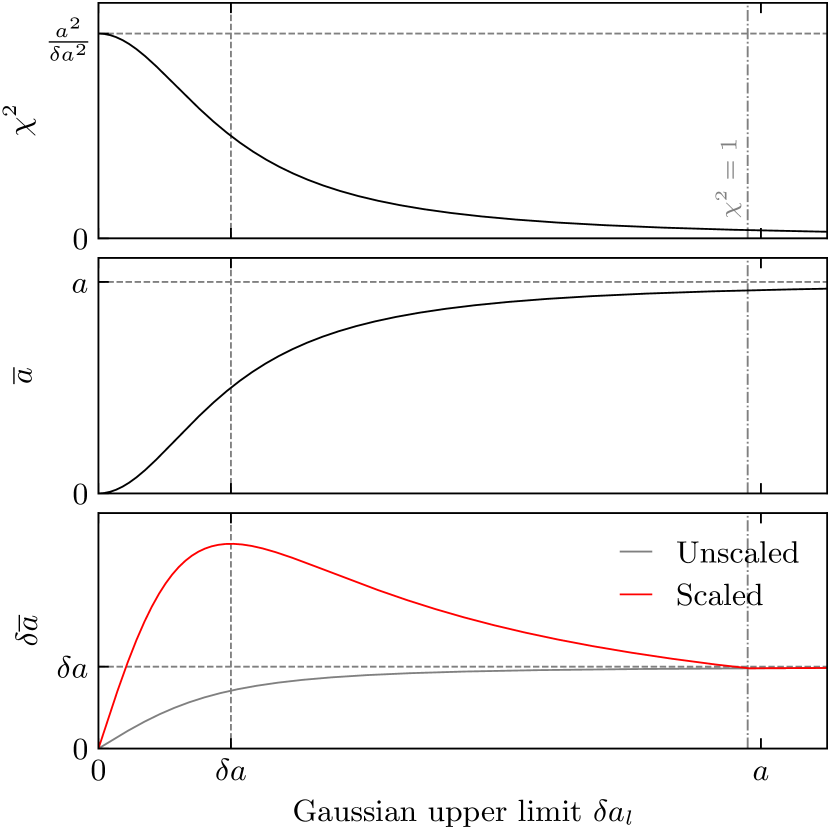
The levels of 232Th and 238U in the Demonstrator’s components often lie below the detection limits of the most sensitive assays, leading to a high prevalence of upper limits. The motivation to include upper limits, not only in the sum of Eq. 2 but also in the calculation of the scaling factor , stems from this prevalence. To justify their use, the effect of combining an upper limit, , with a fixed measured value, , with small error (), was evaluated. This case is representative of many assay results. Fig. 2 shows the , average and uncertainty with respect to a Gaussian upper limit, , between 0 and . It demonstrates that averaging with an upper limit leads to the following desirable properties:
-
1.
For , and rapidly converge to and respectively. Smaller lead to faster convergence. In other words, upper limits higher than measured values have little effect on the same. The lower the measured value’s error, the lower the impact. In this regime .
-
2.
For , decreases monotonically with .
-
3.
The uncertainty, is maximized when . For this value, . Note the importance of scaling the uncertainty and thus the need to include the upper limit in the calculation of .
If assays have to be averaged more than once, multiple upper limits may contribute to the result. For example, 40 of the Demonstrator’s lead bricks were assayed with the following procedure. One or more samples were taken from each brick, and each sample was used to prepare one or more dilutions to conduct ICPMS measurements. In some cases each dilution was separated into multiple vials, which were separately measured. Thus averaging is performed at the dilution, sample, brick and global levels, with upper limits contributing at each stage.
The specific activity averages and uncertainties of the materials used in the Majorana Demonstrator are presented in Table 1. These values are used to calculate the BI contributions of all 232Th and 238U sources used to model the experiment. In this table, represents the number of assays contributing at the global averaging level. While the set of assayed components is limited, it is assumed to be representative of all those used in the Demonstrator.
| Material | Group | 232Th [Bq/kg] | 238U [Bq/kg] | Method | |
|---|---|---|---|---|---|
| LMFE | Front Ends | 6950 830 | 10600 300 | 2 | ICPMS |
| HV Cable | Cables | 87.9 52.4 | 231 34 | 3 | ICPMS |
| Signal Cable | Cables | 546 112 | 530 58 | 3 | ICPMS |
| Stock UGEFCu | Electroformed Cu | 0.188 0.029 | 0.137 0.044 | 5 | ICPMS |
| Machined UGEFCu | Electroformed Cu | 0.575 0.088 | 0.752 0.083 | 12 | ICPMS |
| OFHCCu | OFHC Cu Shielding | 1.10 0.14 | 1.37 0.18 | 2 | ICPMS |
| Pb Bricks | Pb Shielding | 9.53 1.01 | 25.6 1.5 | 29, 19 | ICPMS |
| Female Connector | Connectors | 390 7 | 540 9 | 1 | ICPMS |
| Male Connector | Connectors | 28.8 2.0 | 130 11 | 1 | ICPMS |
| PTFE O-ring | Other Plastics | 39.7 31.9 | 105 | 2, 1 | NAA |
| PTFE | Detector Unit PTFE | 0.101 0.008 | 4.97 | 1 | NAA |
| DuPontTM Vespel® | Other Plastics | 360 234 | 403 179 | 3 | ICPMS |
| PTFE Gasket | Other Plastics | 20.7 | 94.5 | 1 | NAA |
| Stainless Steel | Vacuum Hardware | 13000 4000 | 5000 | 1 | -count |
| Glass Break | Vacuum Hardware | 49000 8000 | 160000 10000 | 1 | -count |
| PTFE Tubing | Other Plastics | 6.09 7.30 | 38.6 | 1 | ICPMS |
| Parylene | Parylene | 2150 120 | 3110 750 | 1 | ICPMS |
IV Background index
Simulations predict an approximately flat background in the 370 keV split BEW covering 1950-2350 keV. The BEW has three 10 keV regions removed, centered at 2103 keV, the 208Tl (232Th) single escape peak, and 2118 keV and 2204 keV, the 214Bi (238U) peaks. This BEW is used to estimate the BI at , for both simulations and data. When estimating the BI from data an additional 10 keV region, centered at , is removed [1].
The contribution to the Demonstrator’s BI from a natural radiation source – the 232Th or 238U contamination in a component of mass – is calculated as follows. For each segment, , of the decay chain of the source’s contaminant, MaGe simulates decays. For a given source , all are equal up to computational errors. Simulated events leading to energy depositions in an operational detector are subject to the same anti-coincidence and pulse shape analysis cuts applied to data (designed to select -like single-site events). The number of counts passing all cuts, , is calculated by integrating the resulting combined detector spectra over the BEW. The corresponding segment efficiency is thus:
| (4) |
The segment efficiencies are weighted by the branching ratio of each segment, , and summed over the total number of segments, , to produce the source efficiency, :
| (5) |
The source efficiency, mass and averaged specific activity, , are used to calculate the BI of the source:
| (6) |
Where keV is the width of the BEW and is the mass of operational detectors in the array. Note that the total number of sources is equal to twice the number of components used to model the Demonstrator, since 232Th and 238U are accounted for in all components. The source contributions to the total , can be summed as desired, either by source material, contaminant, or component group. If only an upper limit, , is available, it can be used in place of . This calculates a BI which is the direct sum of upper limits and central values and is referred to as the direct BI in the text. The component-group-combined 232Th and 238U direct BIs are calculated by summing over the appropriate sources and are presented in Table 2. Note that the design geometry projection of Ref. [15] used this method. It is not possible to assign an uncertainty to the direct BI because of the inclusion of upper limits. However, a proper treatment of uncertainties can be obtained by promoting the single-valued (or ), and to distributions and using Monte Carlo uncertainty propagation to combine these in a final BI distribution.
V Promoting single values to distributions
As described in Section III the specific activity can be expressed as a truncated-at-zero Gaussian. The mass, , is also promoted to a distribution of this form. Depending on the method used to measure or estimate the mass, a Gaussian uncertainty is assigned. This uncertainty ranges from 1%, to account for sample to sample variation in direct mass measurements, to 10% for masses that were estimated from geometry. In practice the mass PDFs are indistinguishable from a true Gaussian given the assigned level of uncertainty.
The derivation of the efficiency, , PDF follows. Starting from Eq. 4, the probability of finding counts in the BEW – with expectation value – is given by the Poisson distribution, . Conversely, is deduced via Bayes’ theorem, , using the prior,
| (7) |
The choice of uninformative prior corresponds to a flat prior on the sum of the decay chain segments. The functional form of the prior is derived in Appendix A.
| (8) |
The resulting posterior is a Gamma distribution with parameters and . The probability of obtaining an efficiency , given an ensemble of counts is thus,
| (9) |
This result is obtained by replacing by in Eq. 4 and carrying it into Eq. 5. The PDF of is computed numerically. Taking a random draw from the PDF in Eq. V for each segment, weighing by the appropriate factors and summing them as in Eq. V. This process is repeated times to generate the PDF or only once if one efficiency sample is needed.
Not all segments are included in the sum for far away sources, only segments which produce ’s with sufficiently high energies to lead to energy depositions in the BEW. The excluded segments have a true zero efficiency.
VI Monte Carlo uncertainty propagation
The assay-based background index can be promoted to a distribution by sampling the PDFs described in Section V. The distributions are thus generated in a similar manner as that of the efficiency. A random draw is taken from the specific activity, mass, and efficiency PDFs. These are multiplied and scaled as in Eq. 6. The process is repeated times to produce a PDF for the BI of the source. Each set of draws constitutes a toy experiment resulting in a different BI. The uncertainty of the efficiency, specific activity and mass – embedded in their corresponding PDFs – is propagated into the distribution through this process, referred to as Monte Carlo uncertainty propagation.
The PDFs are combined by taking the direct sum of the samples that were used to generate them. Fig. 3 shows the result of summing all the PDFs belonging to a component group in the Demonstrator. The mean and uncertainties that are extracted from these distributions are reported in Table 2 and plotted as error bars in Fig. 3. The total BI distribution of 232Th and 238U sources in the Demonstrator is computed in a similar manner and displayed at the bottom of the figure.
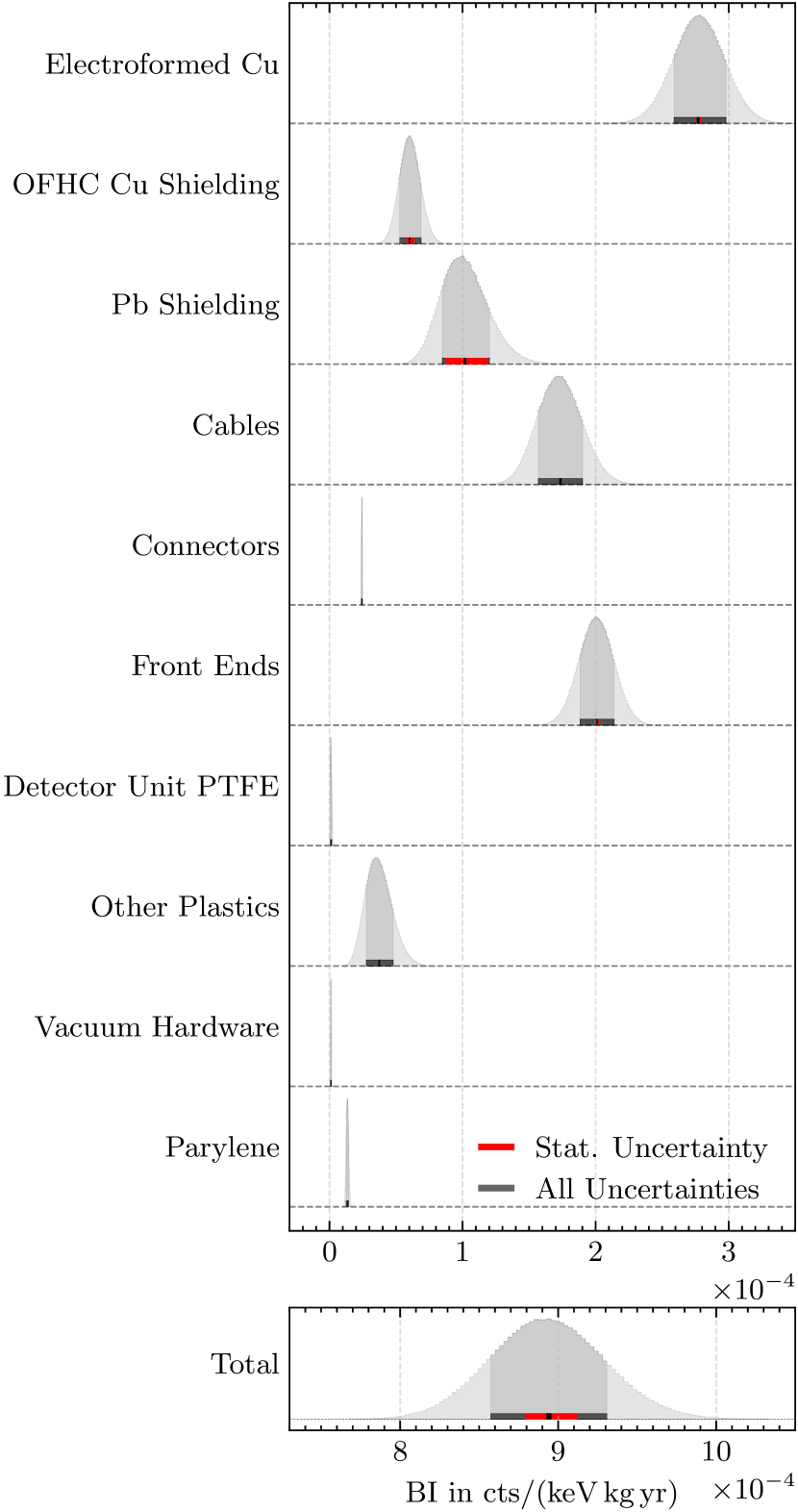
Simulation statistical uncertainties can be isolated by collapsing the specific activity and mass distributions to their respective means and using them to weigh the samples that were drawn from the efficiency distribution. This information can be used by the analyst as a guide to set the number of decays in future simulations.
Monte Carlo uncertainty propagation allows for all potential sources of natural radiation to be incorporated in the model, not just those which produced counts in the BEW. With no counts in the BEW, the single-valued efficiency is zero. However, the efficiency distribution will take an exponential form, effectively setting an upper limit on the BI (once weighted properly) for the source in question. This upper limit is fully dependent on the number of simulated decays and given enough computational resources should be driven down to the point where it is negligible compared to other contributions to the BI. This is the case for the Vacuum Hardware and Pb Shielding 238U contamination.
| Group | Mean 232Th BI | Mean 238U BI | Mean BI | Direct BI |
|---|---|---|---|---|
| [cts/(keV kg yr)] | [cts/(keV kg yr)] | [cts/(keV kg yr)] | [cts/(keV kg yr)] | |
| Electroformed Cu | ||||
| OFHC Cu Shielding | ||||
| Pb Shielding | ||||
| Cables | ||||
| Connectors | ||||
| Front Ends | ||||
| Detector Unit PTFE | ||||
| Other Plastics | ||||
| Vacuum Hardware | ||||
| Parylene | ||||
| SUM |
VII Projected background and conclusions
As Section VI describes, the mean BI and the corresponding uncertainties of the Majorana Demonstrator’s component groups are extracted from their distributions in Fig. 3 and reported in Table 2. The mean total natural radiation BI, determined from its distribution at the bottom of the figure, is
in units of cts/(keV kg yr). The uncertainty from activity (act.) dominates and most component group BIs. The statistical uncertainty from simulation (stat.) has been calculated with the method described in Section VI. Note that the symmetric uncertainty around the mean does not capture the asymmetry of the distribution. The contributions from the 232Th and 238U decay chains, given in units of cts/(keV kg yr), follow:
By comparing the direct BI of Table 2 with the design geometry projection of Ref. [15] for the same components, a 44% increase is found. Uncertainties were not calculated for the design geometry projection. On the other hand, Monte Carlo uncertainty propagation captured the uncertainties from specific activity, component mass and simulation efficiencies in the BI. Multiple contaminants, which have null single-valued efficiencies, contribute to the BI under this new framework.
The projected does not capture the uncertainty associated with the assumption of secular equilibrium or account for the possible introduction of backgrounds during the construction of the Demonstrator. Additionally, given the limited number of assayed components, the variation in contaminants may be larger than captured by the averaged assay uncertainty. Furthermore, possible systematic uncertainties in simulated component geometry were not taken into account. Nevertheless, the Monte Carlo uncertainty propagation framework that has been developed can be extended to account for these effects.
The techniques outlined in this article can be exploited to project the BI of future experiments. Particularly, the design of such experiments can benefit from the ability to include component mass uncertainties, since the designed and as-built geometries often differ. Additionally, the framework informs the analyst on the number of decays to simulate, thus optimizing computational resources. The unified approach to average assay results can facilitate the standardization of assay reporting. This is of importance in the field, given that the design of new experiments often draws from assay data collected by others. The uncertainty extracted from the BI can be propagated into the projected sensitivity, thus further illuminating the physics reach of the next generation of experiments.
Acknowledgments
This material is based upon work supported by the U.S. Department of Energy, Office of Science, Office of Nuclear Physics under contract / award numbers DE-AC02-05CH11231, DE-AC05-00OR22725, DE-AC05-76RL0130, DE-FG02-97ER41020, DE-FG02-97ER41033, DE-FG02-97ER41041, DE-SC0012612, DE-SC0014445, DE-SC0017594, DE-SC0018060, DE-SC0022339, and LANLEM77/LANLEM78. We acknowledge support from the Particle Astrophysics Program and Nuclear Physics Program of the National Science Foundation through grant numbers MRI-0923142, PHY-1003399, PHY-1102292, PHY-1206314, PHY-1614611, PHY-1812409, PHY-1812356, PHY-2111140, and PHY-2209530. We gratefully acknowledge the support of the Laboratory Directed Research & Development (LDRD) program at Lawrence Berkeley National Laboratory for this work. We gratefully acknowledge the support of the U.S. Department of Energy through the Los Alamos National Laboratory LDRD Program, the Oak Ridge National Laboratory LDRD Program, and the Pacific Northwest National Laboratory LDRD Program for this work. We gratefully acknowledge the support of the South Dakota Board of Regents Competitive Research Grant. We acknowledge the support of the Natural Sciences and Engineering Research Council of Canada, funding reference number SAPIN-2017-00023, and from the Canada Foundation for Innovation John R. Evans Leaders Fund. We acknowledge support from the 2020/2021 L’Oréal-UNESCO for Women in Science Programme. This research used resources provided by the Oak Ridge Leadership Computing Facility at Oak Ridge National Laboratory and by the National Energy Research Scientific Computing Center, a U.S. Department of Energy Office of Science User Facility. We thank our hosts and colleagues at the Sanford Underground Research Facility for their support.
Appendix A Efficiency distribution prior derivation
The choice of prior, , becomes apparent here when all , , are equal for a given in Eq. 5. Setting and dropping the indices, the sum to be evaluated is . The sum of PDFs is given by their convolution. Defining the convolution with itself times as
| (10) |
and rewriting as , an unknown function to be solved for, the sum becomes the following convolution:
| (11) |
If the decay chain was simulated as a whole and not by segment, would be given by Eq. V but with and . The functional form of must be such that the sum of the PDFs of the segments equals the PDF of the full decay chain:
| (12) |
Taking the Laplace transform and working simultaneously on both sides yields:
| (13) |
Eq. A has the same functional form as Eq. V up to a constant. Therefore when , , are equal for a given , the prior must take the form . The use of this prior is extended to all cases.
References
- Arnquist et al. [2023] I. J. Arnquist et al. (Majorana Collaboration), Phys. Rev. Lett. 130, 062501 (2023).
- Agostini et al. [2020] M. Agostini et al. (GERDA Collaboration), Phys. Rev. Lett. 125, 252502 (2020).
- Abe et al. [2023] S. Abe et al. (KamLAND-Zen Collaboration), Phys. Rev. Lett. 130, 051801 (2023).
- Anton et al. [2019] G. Anton et al. (EXO-200 Collaboration), Phys. Rev. Lett. 123, 161802 (2019).
- Adams et al. [2022] D. Q. Adams et al. (CUORE Collaboration), Nature 604, 53 (2022).
- Abgrall et al. [2017] N. Abgrall et al. (LEGEND collaboration), AIP Conf. Proc. 1894, 020027 (2017), arXiv:1709.01980 [physics.ins-det] .
- Adhikari et al. [2021] G. Adhikari et al. (nEXO Collaboration), Journal of Physics G: Nuclear and Particle Physics 49, 015104 (2021).
- Alfonso et al. [2022] K. Alfonso et al. (CUPID Collaboration), Journal of Low Temperature Physics 211, 10.1007/s10909-022-02909-3 (2022).
- Avignone et al. [2005] F. T. Avignone, G. S. King, and Y. G. Zdesenko, New Journal of Physics 7, 6 (2005).
- Avignone et al. [2008] F. T. Avignone, S. R. Elliott, and J. Engel, Rev. Mod. Phys. 80, 481 (2008).
- Abgrall et al. [2018] N. Abgrall et al. (MAJORANA), Nucl. Instrum. Meth. A 877, 314 (2018), arXiv:1707.06255 [physics.ins-det] .
- Avignone III and Elliott [2019] F. T. Avignone III and S. R. Elliott, Frontiers in Physics 7, 6 (2019).
- Rahaman et al. [2008] S. Rahaman, V.-V. Elomaa, T. Eronen, J. Hakala, A. Jokinen, J. Julin, A. Kankainen, A. Saastamoinen, J. Suhonen, C. Weber, and J. Äystö, Physics Letters B 662, 111 (2008).
- Douysset et al. [2001] G. Douysset, T. Fritioff, C. Carlberg, I. Bergström, and M. Björkhage, Phys. Rev. Lett. 86, 4259 (2001).
- Abgrall et al. [2016a] N. Abgrall et al. (Majorana Collaboration), Nuclear Instruments and Methods in Physics Research Section A: Accelerators, Spectrometers, Detectors and Associated Equipment 828, 22 (2016a).
- Alduino et al. [2017] C. Alduino et al. (Cuore Collaboration), The European Physical Journal C 77, 543 (2017).
- Albert et al. [2018] J. B. Albert et al. (nEXO Collaboration), Phys. Rev. C 97, 065503 (2018).
- Tsang et al. [2018] R. H. M. Tsang, I. J. Arnquist, E. W. Hoppe, J. L. Orrell, and R. Saldanha, (2018), arXiv:1808.05307 [physics.data-an] .
- Abgrall et al. [2014] N. Abgrall et al. (Majorana Collaboration), Advances in High Energy Physics 2014, 365432 (2014).
- Heise [2015] J. Heise, Journal of Physics: Conference Series 606, 012015 (2015).
- Hoppe et al. [2014] E. Hoppe, C. Aalseth, O. Farmer, T. Hossbach, M. Liezers, H. Miley, N. Overman, and J. Reeves, Nuclear Instruments and Methods in Physics Research Section A: Accelerators, Spectrometers, Detectors and Associated Equipment 764, 116 (2014).
- Bugg et al. [2014] W. Bugg, Y. Efremenko, and S. Vasilyev, Nuclear Instruments and Methods in Physics Research Section A: Accelerators, Spectrometers, Detectors and Associated Equipment 758, 91 (2014).
- Abgrall et al. [2022] N. Abgrall et al. (Majorana Collaboration), Journal of Instrumentation 17 (05), T05003.
- Abgrall et al. [2016b] N. Abgrall et al. (Majorana Collaboration), Nuclear Instruments and Methods in Physics Research Section A: Accelerators, Spectrometers, Detectors and Associated Equipment 823, 83 (2016b).
- Boswell et al. [2011] M. Boswell et al., IEEE Transactions on Nuclear Science 58, 1212 (2011).
- Alvis et al. [2019] S. I. Alvis et al. (Majorana Collaboration), Phys. Rev. C 100, 025501 (2019).
- Gilliss [2019] T. F. Gilliss, ProQuest Dissertations and Theses , 165 (2019).
- Agostini et al. [2017] M. Agostini et al., Limits on uranium and thorium bulk content in gerda phase i detectors, Astroparticle Physics 91, 15 (2017).
- Workman et al. [2022] R. L. Workman et al. (Particle Data Group), PTEP 2022, 083C01 (2022).