Density-Dependent Gauge Field with Raman Lattices

Abstract

The study of the gauge field is an everlasting topic in modern physics. Spin-orbit coupling is a powerful tool in ultracold atomic systems, resulting in an artificial gauge field that can be easily manipulated and observed in a tabletop environment. Combining optical lattices and atom-atom interaction, the artificial gauge field can be made density-dependent. In this work, we investigate a one-dimensional Bose-Hubbard model with spin-orbit coupling, where a density-dependent gauge field emerges spontaneously in low-energy physics. First, we focus on the two-body quantum walk dynamics and give an interpretation of the phenomena with resonant tunneling. Then, we calculate the mean-field phase diagram using the two-site Gutzwiller ansatz. Two types of superfluid phase and a Mott insulator phase are found. Finally, we discuss the experimental realization protocol with Raman lattices.

I Introduction

Gauge theory is the cornerstone of modern physics. Elementary particles interact with each other through gauge fields, which is at the heart of the standard model Weinberg (1995); Gattringer and Lang (2010); Yang et al. (2020). In high energy physics, gauge fields are governed by physical laws, and the study of gauge fields involves accelerating particles and observe their collision Ellis et al. (1996); Su et al. (2024). In solid-state systems, artificial gauge fields can be exerted externally Klitzing et al. (1980); Laughlin (1981); Thouless et al. (1982) or designed intrinsically Haldane (1988); Qi et al. (2006); Chang et al. (2013), which would result in topological bands and lead to novel materials with vast application potential Chang et al. (2023). Alternatively, gauge fields can be simulated within ultracold atom systems, by manipulating the geometry phase the atoms acquired while interacting with light Dalibard et al. (2011); Goldman et al. (2014); Cooper et al. (2019). The simulation of gauge theory in ultracold atom systems has been a fruitful area of study throughout the years, with plenty of proposals Dum and Olshanii (1996); Visser and Nienhuis (1998); Dutta et al. (1999); Juzeliūnas et al. (2005); Osterloh et al. (2005); Ruseckas et al. (2005); Juzeliūnas et al. (2006); Zhu et al. (2006); Günter et al. (2009); Spielman (2009); Campbell et al. (2011); Anderson et al. (2012); Xu and You (2012) and experiments Madison et al. (2000); Lin et al. (2009a, b, 2011a); Aidelsburger et al. (2013); Atala et al. (2013); Miyake et al. (2013); Parker et al. (2013); Struck et al. (2013) to create and observe artificial gauge fields such as spin-orbit coupling (SOC). In particular, the realization of SOC induced by Raman transitions enables new ways to study topological bands and gauge fields Lin et al. (2011b); Zheng and Li (2012); Zheng et al. (2013); Ji et al. (2014); Zheng and Zhai (2014); Wu et al. (2016); Huang et al. (2016); Zhang and Zhou (2017); Lang et al. (2017); Hasan et al. (2022); Liang et al. (2023), where 2D SOC can lead to the Qi-Wu-Zhang model Qi et al. (2006); Wu et al. (2016); Sun et al. (2018a, b); Liang et al. (2023) and 3D SOC results in an ideal Weyl semimetal Wang et al. (2021).

In some of the quantum simulations of artificial gauge fields mentioned above, the gauge fields may be static, only providing a background stage for matter’s evolution. Recently, the focus of the study has advanced to the simulation of the dynamical gauge field, which is more of an analog to the real gauge fields in the physical world Clark et al. (2018); Görg et al. (2019); Schweizer et al. (2019); Yang et al. (2020); Frölian et al. (2022); Yao et al. (2022). In these systems, atoms (matter) give a back action to the gauge field. Therefore, the gauge field is no longer a background field but a degree of freedom evolving self-consistently. One practical way to create a dynamical gauge field is to make the gauge potential density-dependent using atom-atom interaction. After the groundbreaking realization of spin-orbit coupling with ultracold atoms Lin et al. (2011b), there has been a vast number of theoretical studies that introduce on-site interaction to spin-orbit coupled bosons in lattices Cole et al. (2012); Radić et al. (2012); Bolukbasi and Iskin (2014); Hickey and Paramekanti (2014); Zhao et al. (2014a, b); Xu et al. (2021). These works investigated the ground state spin texture as well as the phase transitions that was brought about by spin-orbit coupling. Recently, a proposal was made to create non-Abelian dynamical gauge field and topological superfluids for fermions with optical Raman lattices Zhou et al. (2023). However, the density-dependent gauge field generated by spin-orbit coupling in a Bose-Hubbard landscape has yet been covered.

In this work, we start from a one-dimensional Bose-Hubbard model with spin-orbit coupling. In the strong interaction regime, a density-dependent gauge field emerges spontaneously in low-energy physics. First, we investigate the two-body quantum walk dynamics. Within different parameter regimes and initial states, the time evolution and spin-spin correlation functions show different behaviors, such as asymmetric tunneling, confinement, etc. Further, we study the many-body ground state phase diagram with a clustered Gutzwiller method. Apart from the ordinary Mott insulator (MI) phase and superfluid (SF) phase, an extra MSF (magnetic superfluid) phase has been found. Finally, we give an initial experimental protocol based on Raman lattices and a deep optical lattice to realize the spin-orbit coupling and the Hubbard interaction.

II Model

We consider a one-dimensional Bose-Hubbard model with spin-orbit coupling. The Hamiltonian can be written as Wu et al. (2016); Wang et al. (2018)

$$\hat{H}_{\mathrm{Hubbard}}= \hat{H}_{0}+\hat{H}_{\mathrm{int}}-\mu\hat{n}_{j},$$ (1)

$$\hat{H}_{0}= \sum_{j}(\hat{\mathbf{\Psi}}_{j}^{\dagger}\frac{\delta}{2}\sigma_{z}\hat{\mathbf{\Psi}}_{j}+\hat{\mathbf{\Psi}}_{j\pm 1}^{\dagger}T_{j}^{\pm}\hat{\mathbf{\Psi}}_{j}),$$

$$\hat{H}_{\mathrm{int}}= \sum_{j}[\frac{U_{\uparrow\uparrow}}{2}\hat{n}_{j\uparrow}(\hat{n}_{j\uparrow}-1)+\frac{U_{\downarrow\downarrow}}{2}\hat{n}_{j\downarrow}(\hat{n}_{j\downarrow}-1)+U_{\uparrow\downarrow}\hat{n}_{j\uparrow}\hat{n}_{j\downarrow}],$$

where $\delta/2$ is the Zeeman splitting, $T_{j}^{\pm}=t_{0}\sigma_{z}\mp it_{\mathrm{SO}}\sigma_{x}$ are the tunneling matrices, $t_{0}$ $(t_{\mathrm{SO}})$ is the spin-conserved (spin-flipped) tunneling strength, $U_{\sigma\sigma^{\prime}}(\sigma=\uparrow,\downarrow)$ are the spin dependent on-site interaction strengths, $\mu$ is the chemical potential, $\hat{\mathbf{\Psi}}^{\dagger}_{j}=(\hat{c}^{\dagger}_{j\uparrow},\hat{c}^{\dagger}_{j\downarrow})$ denotes the creation operators of the spinful bosons, $\hat{n}_{j\sigma}=\hat{c}^{\dagger}_{j\sigma}\hat{c}_{j\sigma}$ is the number operator, $\hat{n}_{j}=\hat{n}_{j\uparrow}+\hat{n}_{j\downarrow}$, $\sigma_{x,z}$ are the Pauli matrices. In a Hubbard model, the on-site interaction energy depends on the occupation. Thus, generally speaking, large interaction can strongly suppress the tunneling process. However, in our system, the spin-flipped tunneling can be restored by a Raman process with two-photon detuning $\delta\sim U$, so that the overhead energy from a spin flip can be compensated by the interaction energy difference of tunneling Jürgensen et al. (2014); Xu et al. (2018). Therefore, the spin-conserved and flipped tunneling can happen depending on the density difference between the two sites.

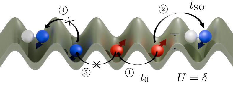
Figure 1: Physical picture of the density-dependent tunneling. Red balls with upward arrows denote spin-up atoms, while blue ones with arrows pointing down are spin-down atoms. The white ball represents an arbitrary spin. The spin-up state and the spin-down state have an energy difference $\delta$ due to the Zeeman splitting. This energy difference can be compensated by the interaction energy change $U$ when atoms tunnel to neighboring sites. For examples of tunneling labeled as \scriptsize{1}⃝ to \scriptsize{4}⃝ help to illustrate the density-dependent tunneling (see main text).

Under a unitary transformation and rotating-frame approximation sup (a), the Hamiltonian turns into

$$\hat{H}_{\mathrm{DD}}=\sum_{j}[\hat{\mathbf{\Psi}}_{j\pm 1}^{\dagger}T_{\mathrm{DD}}^{\pm}\hat{\mathbf{\Psi}}_{j}+\frac{\tilde{U}_{\uparrow\uparrow}}{2}\hat{n}_{j\uparrow}(\hat{n}_{j\uparrow}-1)+\frac{\tilde{U}_{\downarrow\downarrow}}{2}\hat{n}_{j\downarrow}(\hat{n}_{j\downarrow}-1)+\tilde{U}_{\uparrow\downarrow}\hat{n}_{j\uparrow}\hat{n}_{j\downarrow}-\mu\hat{n}_{j}],$$ (2)

in which the tunneling matrix becomes density-dependent,

$$T^{\pm}_{\mathrm{\mathrm{DD}}}=\begin{pmatrix}\hat{P}^{0}_{\pm}t_{0}&\mp\hat{P}^{-1}_{\pm}t_{\mathrm{SO}}\\ \pm\hat{P}^{+1}_{\pm}t_{\mathrm{SO}}&-\hat{P}^{0}_{\pm}t_{0}\end{pmatrix}.$$ (3)

$\hat{P}^{\Delta n}_{\pm}=\sum_{n}\hat{P}^{n+\Delta n}_{j\pm 1}\hat{P}^{n}_{j}$ is the projection operator, projecting the system into the subspace where atom numbers differ in $\Delta n$ between neighboring sites. $\tilde{U}_{\sigma\sigma^{\prime}}=U_{\sigma\sigma^{\prime}}-\delta$ are the effective interaction strengths. Figure 1 shows the physical picture of the density-dependent tunneling. In our system, whether a tunneling process can happen depends on the density difference between the two sites. The tunneling can be illustrated with four different processes. Figure 1.\scriptsize{1}⃝ shows a spin-up atom tunneling to a neighboring empty site with its spin conserved. There’s no energy change whatsoever, the process is on-resonance. This also applies to spin-down atoms. Figure 1.\scriptsize{2}⃝ is a spin-up atom tunneling to a neighboring single-occupied site and flipping spin. The interaction energy increases by $U$, which can be compensated by the Zeeman energy change $\delta$ if $U=\delta$. Therefore, this process is on-resonance. Its reverse process, namely a spin-down atom in a double-occupied site tunneling to a neighboring empty site and flipping spin, is also on-resonance. These are the only allowed dynamics. Figure 1.\scriptsize{3}⃝ shows a spin-up atom tunneling to a neighboring empty site and flipping spin. This will result in an energy change by $\delta$, meaning the process is off-resonance. Finally, a spin-down atom tunneling to a neighboring single-occupied site without flipping spin, shown in figure 1.\scriptsize{4}⃝, will lead to a change in interaction energy by $U$, which also makes the process off-resonance.

III Quantum Walk

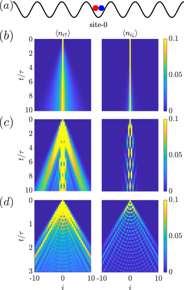
Figure 2: Time evolution of initial state $|\dots,0,0,\uparrow\downarrow,0,0,\dots\rangle$. (a) Sketch of the initial state. Red circle represents a spin-up atom, blue circle represents a spin-down atom. (b-d) Density evolution of spin up and spin down at $t_{\mathrm{SO}}/t_{0}=0.1,1,10$. The cut-off time for $t_{\mathrm{SO}}/t_{0}=10$ is chosen at $t=3\tau$ since the atoms are approaching the boundaries.

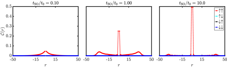
Figure 3: Distance correlation function $\mathcal{C}_{\sigma,\sigma^{\prime}}(r)$ of initial state $|\dots,0,0,\uparrow\downarrow,0,0,\dots\rangle$ and different $t_{\mathrm{SO}}$. The zero-distance data $\mathcal{C}_{\sigma,\sigma^{\prime}}(0)$ is omitted due to its elevated value.

To study the density-dependent effect, we first consider the two-body quantum walk. Specifically, we start with a spin-up and a spin-down atom at different initial sites and investigate their dynamics under different parameters. In this section, we set $U_{\uparrow\uparrow}=U_{\downarrow\downarrow}=U_{\uparrow\downarrow}=\delta$ for simplicity, i.e. $\tilde{U}_{\sigma\sigma^{\prime}}=0$, and focus only on the effect of the density-dependent tunneling. The chemical potential $\mu$ is also set to zero. The Hamiltonian becomes

$$\hat{H}_{\mathrm{DD}}=\sum_{j}\hat{\mathbf{\Psi}}_{j\pm 1}^{\dagger}T_{\mathrm{DD}}^{\pm}\hat{\mathbf{\Psi}}_{j}.$$ (4)

We compare two unique initial site configurations: $|\dots,0,0,\uparrow\downarrow,0,0,\dots\rangle$ and $|\dots,0,0,\uparrow,\downarrow,0,0,\dots\rangle$. The former is two atoms of opposite spin starting from the same site, and the latter is from neighboring sites. In each case, the spin-conserved tunneling strength $t_{0}$ is fixed, while the spin-flipped tunneling strength $t_{\mathrm{SO}}/t_{0}$ varies in 0.1, 1, and 10. We calculate the dynamics along a chain from $t=0$ to $t=10\tau$, $\tau=1/t_{0}$. (For $t_{\mathrm{SO}}/t_{0}=1$ in the first configuration, we stop the calculation at $t=3\tau$ since the atoms arrive at the edges earlier.) We present the density distribution of the two spins at each time, as well as the two-body correlation function $\mathcal{C}_{\sigma,\sigma^{\prime}}(r)=\sum_{i}\langle n_{i\sigma}n_{(i+r)\sigma^{\prime}}\rangle$ ($\sigma$,$\sigma^{\prime}$=$\uparrow$ or $\downarrow$) at the end of the dynamics Kwan et al. (2023). Here we integrate out the center-of-mass index and focus on the correlation over relative distance $r$. In these results, we can see how the density-dependent tunneling affects the evolution and leads to confinement between two spins. We also find different propagation behaviors for different configurations that are unique for our density-dependent system sup (b).

The first case is $|\dots,0,0,\uparrow\downarrow,0,0,\dots\rangle$, i.e. a spin-up atom and a spin-down atom starting at site $0$. The density evolution is shown in figure 2. For $t_{\mathrm{SO}}/t_{0}=0.1$, the spin-conserved tunneling is dominant. In this case, the start of the dynamics can only happen once the spin-down atom flips spin and hops to the neighboring site. After that, the two atoms are both spin up and can propagate away due to large $t_{0}$. This explains the localized distribution of spin down. If we increase $t_{\mathrm{SO}}/t_{0}$ to 1, the spin-flipped tunneling will be enhanced. The spin-down atom can flip out, after which it can either flip back to site $0$, or start propagating as spin up. On the other hand, once the spin-down atom flips out to site $\pm 1$, the spin-up atom at $0$ can flip inside $\pm 1$, becoming spin down. Further increasing $t_{\mathrm{SO}}/t_{0}$ to $10$, the spin-flipped tunneling will dominate the dynamics. Once the spin-down atom flips out, the other spin-up atom will quickly follow to the same site. Hence the two atoms will be moving as a spin pair.

The correlation function can also give us some insight into the dynamics behavior. For $t_{\mathrm{SO}}/t_{0}=0.1$, the spin up-spin up correlation has an extended profile, the atoms are not confined to each other. When we increase $t_{\mathrm{SO}}/t_{0}$ to $1$, the peak is higher and narrower, which means the system becomes confined. If we tune $t_{\mathrm{SO}}/t_{0}$ to $10$, the system is now strongly confined. Even though the center-of-mass of two atoms is moving quickly, they are bound together.

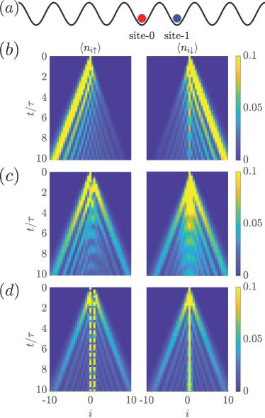
Figure 4: Time evolution of $|\dots,0,0,\uparrow,\downarrow,0,0,\dots\rangle$. (a) Sketch of the initial state. (b-d) Density evolution of spin up and spin down at $t_{\mathrm{SO}}/t_{0}=0,1,1,10$.

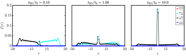
Figure 5: Distance correlation function $\mathcal{C}_{\sigma,\sigma^{\prime}}(r)$ of initial state $|\dots,0,0,\uparrow,\downarrow,0,0,\dots\rangle$ and different $t_{\mathrm{SO}}$. The zero-distance data $\mathcal{C}_{\sigma,\sigma^{\prime}}(0)$ is omitted due to its elevated value.

The second case is $|\dots,0,0,\uparrow,\downarrow,0,0,\dots\rangle$, where two atoms of opposite spins start at neighboring sites. For $t_{\mathrm{SO}}/t_{0}=0.1$, the spin-conserved tunneling is dominant. The two spins need two spin-flip processes to go through one another. Therefore, each spin can propagate to their corresponding half of the lattice, but can hardly cross each other. If we increase $t_{\mathrm{SO}}/t_{0}$ to 1, the spin-flipped tunneling will be enhanced. Different spins can move through one another. This is only made possible by the density-dependent tunneling. Finally, if we set $t_{\mathrm{SO}}/t_{0}$ to $10$, the spin-flipped tunneling becomes the dominant process. The evolution is the superposition of two dynamics: if the evolution starts with the spin-up atom flipping to the spin down site, it will tend to flip back and forth, while the spin down atom remains in situ. If the evolution starts with either atom tunneling to a neighboring empty site, the two atoms will be more likely to propagate freely.

The correlation function can show us how the two spins propagate. When $t_{\mathrm{SO}}/t_{0}=0.1$, two atoms tunnel freely, but only in their own side. The system shows an asymmetric propagation behavior, which is made clear by the asymmetric inter-spin correlation. Note that this asymmetry explicitly comes from the initial state. Increasing $t_{\mathrm{SO}}/t_{0}$ to 1, The correlation function is almost symmetric, because the two spins can move through each other easily. We can also see a confinement peak starting to show up. When $t_{\mathrm{SO}}/t_{0}=10$, the correlation is now mostly around the origin, the two spins are more likely to be bound together. The small plateau corresponds to the free propagation dynamics due to the spin-conserved tunneling.

IV Mean Field Phase Diagram

Next, we come to study the many-body physics and calculate the mean-field phase diagram of the density-dependent Hamiltonian. In this section, we set $\tilde{U}_{\uparrow\uparrow}=\tilde{U}_{\uparrow\downarrow}=\tilde{U}_{\downarrow\downarrow}-\Delta\tilde{U}=\tilde{U}$ as an energy scale. Here we add a small spin imbalance $\Delta\tilde{U}=5\times 10^{-3}\tilde{U}$ to the interaction to explicitly break the $\mathrm{SU}(2)$ symmetry of interaction, similar to ${}^{87}\mathrm{Rb}$ atoms. This can avoid possible degeneracy between doubly occupied states. The density-dependent Hubbard Hamiltonian becomes:

$$\hat{H}_{\mathrm{DD}}=\sum_{j}[\hat{\mathbf{\Psi}}_{j\pm 1}^{\dagger}T_{\mathrm{DD}}^{\pm}\hat{\mathbf{\Psi}}_{j}+\frac{\tilde{U}}{2}\hat{n}_{j}(\hat{n}_{j}-1)\\ +\frac{\Delta\tilde{U}}{2}\hat{n}_{j\downarrow}(\hat{n}_{j\downarrow}-1)-\mu\hat{n}_{j}].$$ (5)

We employ a 2-site clustered Gutzwiller variational wavefunction Lühmann (2013) to find the ground state of the system:

$$|\mathrm{G}\rangle=\prod_{\mathrm{2-site\atop clusters}}\sum_{l_{1\uparrow},l_{1\downarrow},\atop l_{2\uparrow},l_{2\downarrow}}f_{l_{1\uparrow},l_{1\downarrow},l_{2\uparrow},l_{2\downarrow}}|l_{1\uparrow},l_{1\downarrow},l_{2\uparrow},l_{2\downarrow}\rangle,$$ (6)

where $l_{j\uparrow(\downarrow)}$ is the number of atoms at site $j$ with spin up (down). We set the cut-off of atom number of each spin at $l_{j\uparrow(\downarrow)}\leq l_{\mathrm{max}}=2$. The energy of the trial state is $E=\langle\mathrm{G}|\hat{H}|\mathrm{G}\rangle$. The variational parameters $f_{l_{1\uparrow},l_{1\downarrow},l_{2\uparrow},l_{2\downarrow}}$ can be determined by minimizing $E$, with the normalization condition

$$\sum_{l_{1\uparrow},l_{1\downarrow},\atop l_{2\uparrow},l_{2\downarrow}}|f_{l_{1\uparrow},l_{1\downarrow},l_{2\uparrow},l_{2\downarrow}}|^{2}=1.$$ (7)

Our results are shown in figure 6. We found three distinct phases, the Mott insulator (MI) phase, the superfluid (SF) phase, and a new magnetic superfluid (MSF) phase, which is fully polarized.

Figure 6(a-d) show the phase diagrams of $t_{0}/\tilde{U}$ versus $\mu/\tilde{U}$ at $t_{\mathrm{SO}}=0.1\tilde{U}$. The color in (a-b) represents the magnitude of the superfluid order parameter $\langle a_{\uparrow(\downarrow)}\rangle$. In the MI phase, both $\langle a_{\uparrow}\rangle$ and $\langle a_{\downarrow}\rangle$ vanish. In the SF phase, both $\langle a_{\uparrow}\rangle$ and $\langle a_{\downarrow}\rangle$ have non-zero values. In the MSF phase, $\langle a_{\downarrow}\rangle$ is nearly zero, but $\langle a_{\uparrow}\rangle$ is non-zero. From the vertical lines of $t_{0}=0.1$ and $t_{0}=0.4$ (figure 6(e-f)), we can see the phase transitions between the MI phase and the SF/MSF phase are second order phase transitions. The SF-MSF phase transition is first order.

Figure 6: Phase diagrams. (a-b) The magnitude of the superfluid order parameter $\langle a_{\sigma}\rangle$. (c) Phase diagram of the atom number expectation value $\langle n\rangle$. (d) Phase diagram of normalized spin polarization. (e-f) Magnitude of $\langle a\rangle$ along two vertical lines, $t_{0}=0.1\tilde{U}$ and $t_{0}=0.4\tilde{U}$. (g) $\langle n\rangle$ along two vertical lines. (h) Spin polarization $m_{z}$ along two different vertical lines. Our calculation shows that the superfluid order parameter $|\langle a_{j\sigma}\rangle|$ and other observable expectation values are uniform across the two sites. Therefore, we only show the results of the first site of the cluster.

In figure6(d,h) we plot the spin polarization $m_{z}=(\langle n_{\uparrow}\rangle-\langle n_{\downarrow}\rangle)/(\langle n_{\uparrow}\rangle+\langle n_{\downarrow}\rangle)$. The spin in the MSF phase is fully polarized to $\uparrow$, while the SF phase is only partially polarized.

V Experimental Protocol

Our model can be implemented to experiment with Raman lattices and a deep optical lattice. The spin-orbit coupling can be provided with retro-reflected laser beams in the $x-y$ planeWu et al. (2016); Sun et al. (2018b). An additional deep lattice in the $z$ direction can localize the atoms around lattice sites, thus increasing the onsite interaction strength $U$. The Zeeman term $\frac{\delta}{2}$ comes from the two-photon detuning of the Raman lasers. The ratio of $t_{0}$ and $t_{\mathrm{SO}}$ can be tuned by adjusting the polarization of incident Raman beams with wave plates. Finally, a quantum gas microscope can be utilized to probe the quantum walk dynamics and the two body correlation functionPreiss et al. (2015); Kwan et al. (2023). The MI-SF and SF-MSF phase transition can be studied with spin-resolved time of flight (TOF) imaging.

VI Summary

In this work, we constructed a one-dimensional density-dependent dynamical synthetic gauge field from a spin-orbit coupled Bose-Hubbard model. We used a detuned Raman coupling to compensate the on-site interaction and restore the spin-flipped hopping, resulting in a density-dependent tunneling matrix.

Based on this density-dependent Hamiltonian, we first calculated the quantum walk of two opposite spins. We found that by increasing the spin-flipped tunneling strength $t_{\mathrm{SO}}$, two atoms can form a confinement pair. Starting from an spin asymmetric initial state, the density-dependent spin-flipped tunneling can enable atoms of different spins to move through one another, resulting in a symmetric dynamics.

Then, we studied the many-body physics of this density-dependent Hamiltonian. We obtained the mean-field phase diagram with a clustered Gutzwiller method. We found three distinct phases, the MI phase, the SF phase, and a new MSF phase. We found a second-order phase transition between the superfluid phases and the MI phase, and a first-order phase transition between the SF phase and the MSF phase.

Last, we discussed the feasibility of the experimental realization of this model in Raman lattices. We conclude that our prediction can be tested within currently available experimental platforms. We believe that the study of density-dependent dynamical gauge field can be continued along this path to higher dimensions and non-Abelian situations, where more new physics can be found.

Appendix A Derivation of the density-dependent gauge field from the original Bose-Hubbard model

In this appendix, we give a detailed derivation of the unitary transformation that leads to the density-dependent Hamiltonian. Our goal is to formally let the Raman detuning term $\delta/2$ and the interaction term $U_{\sigma,\sigma^{\prime}}$ cancel out, and turn them into phases in the tunneling matrices.

We start with the Bose-Hubbard Hamiltonian (1), and apply the first unitary transformation $G=\mathrm{e}^{i\frac{\delta}{2}t\sum_{j}(\hat{n}_{j\uparrow}-\hat{n}_{j\downarrow})}$. The Hamiltonian reads

$$\hat{H}_{\mathrm{GT}} =G\hat{H}_{\mathrm{Hubbard}}G^{\dagger}-G(i\partial_{t})G^{\dagger}$$ (8)

$$=\sum_{j}[\hat{\Psi}^{\dagger}_{j\pm 1}T^{\pm}_{\mathrm{GT}}\hat{\Psi}_{j}+\frac{U_{\uparrow\uparrow}}{2}\hat{n}_{j\uparrow}(\hat{n}_{j\uparrow}-1)+\frac{U_{\downarrow\downarrow}}{2}\hat{n}_{j\downarrow}(\hat{n}_{j\downarrow}-1)+U_{\uparrow\downarrow}\hat{n}_{j\uparrow}\hat{n}_{j\downarrow}-\mu\hat{n}_{j}],$$

where the tunneling matrices take the form

$$T^{\pm}_{\mathrm{GT}}=t_{0}\sigma_{z}\mp it_{\mathrm{SO}}\begin{pmatrix}0&-i\mathrm{e}^{i\delta t}\\ i\mathrm{e}^{-i\delta t}&0\end{pmatrix}.$$ (9)

Here we can see, the Raman detuning $\delta/2$ turns into a time-dependent phase in the spin-flipped tunneling. We then take the second unitary transformation $R=\mathrm{e}^{i\frac{\delta}{2}t\sum_{j}\hat{n}_{j}(\hat{n}_{j}-1)}$. The Hamiltonian becomes

$$\hat{H}_{\mathrm{DD}} =R\hat{H}_{\mathrm{GT}}R^{\dagger}-R(i\partial_{t})R^{\dagger}$$ (10)

$$=\sum_{j}[\hat{\Psi}^{\dagger}_{j\pm 1}T^{\pm}_{\mathrm{DD}}\hat{\Psi}_{j}+\frac{\tilde{U}_{\uparrow\uparrow}}{2}\hat{n}_{j\uparrow}(\hat{n}_{j\uparrow}-1)+\frac{\tilde{U}_{\downarrow\downarrow}}{2}\hat{n}_{j\downarrow}(\hat{n}_{j\downarrow}-1)+\tilde{U}_{\uparrow\downarrow}\hat{n}_{j\uparrow}\hat{n}_{j\downarrow}-\mu\hat{n}_{j}],$$

where the tunneling matrices are

$$T^{\pm}_{\mathrm{DD}}=\begin{pmatrix}t_{0}\mathrm{e}^{i\delta t\Delta\hat{n}_{j\pm}}&\mp t_{\mathrm{SO}}\mathrm{e}^{i\delta t(\Delta\hat{n}_{j\pm}+1)}\\ \pm t_{\mathrm{SO}}\mathrm{e}^{i\delta t(\Delta\hat{n}_{j\pm}-1)}&-t_{0}\mathrm{e}^{i\delta t\Delta\hat{n}_{j\pm}}\end{pmatrix},$$ (11)

$\Delta\hat{n}_{j\pm}=\hat{n}_{j\pm 1}-\hat{n}_{j}$ is the atom number difference operator between neighboring sites. Here, the tunneling matrices have density-dependent phases, and $\tilde{U}_{\sigma,\sigma^{\prime}}=U_{\sigma,\sigma^{\prime}}-\delta$ is the residual effective interaction. Then, we adopt the rotating-wave approximation to drop the time-dependent oscillating terms, which means projecting the Hamiltonian to the subspace of $\Delta{n}=0,1,-1$, for different elements of the tunneling matrix. Labeling the atom number projection operator on $j$-site $\hat{P}^{n}_{j}$ , and $\hat{P}^{\Delta n}_{\pm}=\sum_{n}\hat{P}^{n+\Delta n}_{j\pm 1}\hat{P}^{n}_{j}$, we finally arrive at the tunneling matrix in (3).

Appendix B Quantum Walk of the Non-Interacting System

In this section, we show the quantum walk dynamics of a non-interacting system without the density dependence in the tunneling matrices. The Hamiltonian is

$$\hat{H}_{\mathrm{NI}} =\sum_{j}\hat{\mathbf{\Psi}}_{j\pm 1}^{\dagger}T_{\mathrm{NI}}^{\pm}\hat{\mathbf{\Psi}}_{j},$$ (12)

$$T^{\pm}_{\mathrm{\mathrm{NI}}} =\begin{pmatrix}t_{0}&\mp t_{\mathrm{SO}}\\ \pm t_{\mathrm{SO}}&-t_{0}\end{pmatrix}.$$

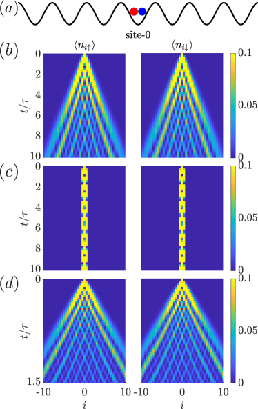
Figure 7: Time evolution of initial state $|\dots,0,0,\uparrow\downarrow,0,0,\dots\rangle$ for the non-interacting system. (a) Sketch of the initial state. Red circle represents a spin-up atom, blue circle represents a spin-down atom. (b-d) Density evolution of spin up and spin down at $t_{\mathrm{SO}}/t_{0}=0.1,1,10$. The cut-off time for $t_{\mathrm{SO}}=10$ is chosen at $t=1.5\tau$ since the atoms are approaching the boundaries.

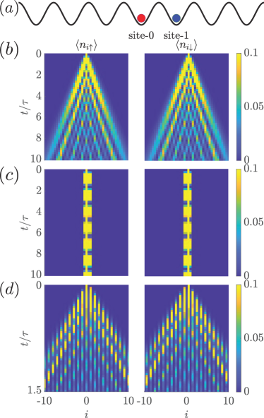
Figure 8: Time evolution of initial state $|\dots,0,0,\uparrow,\downarrow,0,0,\dots\rangle$ for the non-interacting system. (a) Sketch of the initial state. Red circle represents a spin-up atom, blue circle represents a spin-down atom. (b-d) Density evolution of spin up and spin down at $t_{\mathrm{SO}}/t_{0}=0.1,1,10$. The cut-off time for $t_{\mathrm{SO}}=10$ is chosen at $t=1.5\tau$ since the atoms are approaching the boundaries.

Quantum walk evolution for $|\dots,0,0,\uparrow\downarrow,0,0,\dots\rangle$ and $|\dots,0,0,\uparrow,\downarrow,0,0,\dots\rangle$ are shown in figures 7 and 8. We can see that the dynamics is much different without the density dependence. First of all, the dynamics of the two different configurations are very similar, which is not true in the density-dependent case. This is because one of the key distinctions between these two configurations is the density difference among sites, which is fundamental in density-dependent case. However, without density dependence, the dynamics is just wave packet diffusion of two non-interacting atoms. Consequently, some density-dependence-induced dynamics like the asymmetric evolution are not present in the density-independent dynamics, for the atoms have no trouble moving through each other now. Note that the non-propagating dynamics for $t_{\mathrm{SO}}/t_{0}=1$ is the coincidental result of a flat band for these particular parameters.

References

- Weinberg (1995) S. Weinberg, The Quantum Theory of Fields (Cambridge University Press, 1995), 1st ed., ISBN 978-0-521-67053-1 978-0-521-55001-7 978-1-139-64416-7.
- Gattringer and Lang (2010) C. Gattringer and C. B. Lang, Quantum Chromodynamics on the Lattice: An Introductory Presentation, vol. 788 of Lecture Notes in Physics (Springer Berlin Heidelberg, Berlin, Heidelberg, 2010), ISBN 978-3-642-01849-7 978-3-642-01850-3.
- Yang et al. (2020) B. Yang, H. Sun, R. Ott, H.-Y. Wang, T. V. Zache, J. C. Halimeh, Z.-S. Yuan, P. Hauke, and J.-W. Pan, Nature 587, 392 (2020), ISSN 0028-0836, 1476-4687.
- Ellis et al. (1996) R. K. Ellis, W. J. Stirling, and B. R. Webber, QCD and Collider Physics (Cambridge University Press, 1996), 1st ed., ISBN 978-0-521-58189-9 978-0-521-54589-1 978-0-511-62878-8.
- Su et al. (2024) G.-X. Su, J. Osborne, and J. C. Halimeh, A Cold-Atom Particle Collider (2024), eprint 2401.05489.
- Klitzing et al. (1980) K. V. Klitzing, G. Dorda, and M. Pepper, Physical Review Letters 45, 494 (1980), ISSN 0031-9007.
- Laughlin (1981) R. B. Laughlin, Physical Review B 23, 5632 (1981), ISSN 0163-1829.
- Thouless et al. (1982) D. J. Thouless, M. Kohmoto, M. P. Nightingale, and M. Den Nijs, Physical Review Letters 49, 405 (1982), ISSN 0031-9007.
- Haldane (1988) F. D. M. Haldane, Physical Review Letters 61, 2015 (1988), ISSN 0031-9007.
- Qi et al. (2006) X.-L. Qi, Y.-S. Wu, and S.-C. Zhang, Physical Review B 74, 085308 (2006), ISSN 1098-0121, 1550-235X.
- Chang et al. (2013) C.-Z. Chang, J. Zhang, X. Feng, J. Shen, Z. Zhang, M. Guo, K. Li, Y. Ou, P. Wei, L.-L. Wang, et al., Science 340, 167 (2013), ISSN 0036-8075, 1095-9203.
- Chang et al. (2023) C.-Z. Chang, C.-X. Liu, and A. H. MacDonald, Reviews of Modern Physics 95, 011002 (2023), ISSN 0034-6861, 1539-0756.
- Dalibard et al. (2011) J. Dalibard, F. Gerbier, G. Juzeliūnas, and P. Öhberg, Reviews of Modern Physics 83, 1523 (2011), ISSN 0034-6861, 1539-0756.
- Goldman et al. (2014) N. Goldman, G. Juzeliūnas, P. Öhberg, and I. B. Spielman, Reports on Progress in Physics 77, 126401 (2014), ISSN 0034-4885, 1361-6633.
- Cooper et al. (2019) N. R. Cooper, J. Dalibard, and I. B. Spielman, Reviews of Modern Physics 91, 015005 (2019), ISSN 0034-6861.
- Dum and Olshanii (1996) R. Dum and M. Olshanii, Physical Review Letters 76, 1788 (1996), ISSN 0031-9007, 1079-7114.
- Visser and Nienhuis (1998) P. M. Visser and G. Nienhuis, Physical Review A 57, 4581 (1998), ISSN 1050-2947, 1094-1622.
- Dutta et al. (1999) S. K. Dutta, B. K. Teo, and G. Raithel, Physical Review Letters 83, 1934 (1999), ISSN 0031-9007, 1079-7114.
- Juzeliūnas et al. (2005) G. Juzeliūnas, P. Öhberg, J. Ruseckas, and A. Klein, Physical Review A 71, 053614 (2005), ISSN 1050-2947, 1094-1622.
- Osterloh et al. (2005) K. Osterloh, M. Baig, L. Santos, P. Zoller, and M. Lewenstein, Physical Review Letters 95, 010403 (2005), ISSN 0031-9007, 1079-7114.
- Ruseckas et al. (2005) J. Ruseckas, G. Juzeliūnas, P. Öhberg, and M. Fleischhauer, Physical Review Letters 95, 010404 (2005), ISSN 0031-9007, 1079-7114.
- Juzeliūnas et al. (2006) G. Juzeliūnas, J. Ruseckas, P. Öhberg, and M. Fleischhauer, Physical Review A 73, 025602 (2006), ISSN 1050-2947, 1094-1622.
- Zhu et al. (2006) S.-L. Zhu, H. Fu, C.-J. Wu, S.-C. Zhang, and L.-M. Duan, Physical Review Letters 97, 240401 (2006), ISSN 0031-9007, 1079-7114.
- Günter et al. (2009) K. J. Günter, M. Cheneau, T. Yefsah, S. P. Rath, and J. Dalibard, Physical Review A 79, 011604 (2009), ISSN 1050-2947, 1094-1622.
- Spielman (2009) I. B. Spielman, Physical Review A 79, 063613 (2009).
- Campbell et al. (2011) D. L. Campbell, G. Juzeliūnas, and I. B. Spielman, Physical Review A 84, 025602 (2011), ISSN 1050-2947, 1094-1622.
- Anderson et al. (2012) B. M. Anderson, G. Juzeliūnas, V. M. Galitski, and I. B. Spielman, Physical Review Letters 108, 235301 (2012), ISSN 0031-9007, 1079-7114.
- Xu and You (2012) Z. F. Xu and L. You, Physical Review A 85, 043605 (2012), ISSN 1050-2947, 1094-1622.
- Madison et al. (2000) K. W. Madison, F. Chevy, W. Wohlleben, and J. Dalibard, Physical Review Letters 84, 806 (2000), ISSN 0031-9007, 1079-7114.
- Lin et al. (2009a) Y.-J. Lin, R. Compton, A. Perry, W. Phillips, J. Porto, and I. Spielman, Physical Review Letters 102, 130401 (2009a), ISSN 0031-9007, 1079-7114.
- Lin et al. (2009b) Y.-J. Lin, R. L. Compton, K. Jiménez-García, J. V. Porto, and I. B. Spielman, Nature 462, 628 (2009b), ISSN 0028-0836, 1476-4687.
- Lin et al. (2011a) Y.-J. Lin, R. L. Compton, K. Jiménez-García, W. D. Phillips, J. V. Porto, and I. B. Spielman, Nature Physics 7, 531 (2011a), ISSN 1745-2473, 1745-2481.
- Aidelsburger et al. (2013) M. Aidelsburger, M. Atala, M. Lohse, J. T. Barreiro, B. Paredes, and I. Bloch, Physical Review Letters 111, 185301 (2013), ISSN 0031-9007, 1079-7114.
- Atala et al. (2013) M. Atala, M. Aidelsburger, J. T. Barreiro, D. Abanin, T. Kitagawa, E. Demler, and I. Bloch, Nature Physics 9, 795 (2013), ISSN 1745-2473, 1745-2481.
- Miyake et al. (2013) H. Miyake, G. A. Siviloglou, C. J. Kennedy, W. C. Burton, and W. Ketterle, Physical Review Letters 111, 185302 (2013), ISSN 0031-9007, 1079-7114.
- Parker et al. (2013) C. V. Parker, L.-C. C. Ha, and C. Chin, Nature Physics 9, 769 (2013), ISSN 17452481.
- Struck et al. (2013) J. Struck, M. Weinberg, C. Ölschläger, P. Windpassinger, J. Simonet, K. Sengstock, R. Höppner, P. Hauke, A. Eckardt, M. Lewenstein, et al., Nature Physics 9, 738 (2013), ISSN 1745-2473, 1745-2481.
- Lin et al. (2011b) Y.-J. Lin, K. Jiménez-García, and I. B. Spielman, Nature 471, 83 (2011b), ISSN 0028-0836, 1476-4687.
- Zheng and Li (2012) W. Zheng and Z. Li, Phys. Rev. A 85, 053607 (2012).
- Zheng et al. (2013) W. Zheng, Z. Q. Yu, X. Cui, and H. Zhai, Journal of Physics B: Atomic, Molecular and Optical Physics 46 (2013), ISSN 09534075.
- Ji et al. (2014) S.-C. Ji, J.-Y. Zhang, L. Zhang, Z.-D. Du, W. Zheng, Y.-J. Deng, H. Zhai, S. Chen, and J.-W. Pan, Nature Physics 10, 314 (2014), ISSN 1745-2473.
- Zheng and Zhai (2014) W. Zheng and H. Zhai, Phys. Rev. A 89, 061603 (2014).
- Wu et al. (2016) Z. Wu, L. Zhang, W. Sun, X.-T. Xu, B.-Z. Wang, S.-C. Ji, Y. Deng, S. Chen, X.-J. Liu, and J.-W. Pan, Science 354, 83 (2016), ISSN 0036-8075, 1095-9203.
- Huang et al. (2016) L. Huang, Z. Meng, P. Wang, P. Peng, S.-L. Zhang, L. Chen, D. Li, Q. Zhou, and J. Zhang, Nature Physics 12, 540 (2016), ISSN 1745-2473, 1745-2481.
- Zhang and Zhou (2017) S.-L. Zhang and Q. Zhou, Phys. Rev. A 95, 061601 (2017).
- Lang et al. (2017) L.-J. Lang, S.-L. Zhang, and Q. Zhou, Phys. Rev. A 95, 053615 (2017).
- Hasan et al. (2022) M. Hasan, C. S. Madasu, K. D. Rathod, C. C. Kwong, C. Miniatura, F. Chevy, and D. Wilkowski, Physical Review Letters 129, 130402 (2022), ISSN 0031-9007, 1079-7114.
- Liang et al. (2023) M.-C. Liang, Y.-D. Wei, L. Zhang, X.-J. Wang, H. Zhang, W.-W. Wang, W. Qi, X.-J. Liu, and X. Zhang, Physical Review Research 5, L012006 (2023), ISSN 2643-1564.
- Sun et al. (2018a) W. Sun, B.-Z. Wang, X.-T. Xu, C.-R. Yi, L. Zhang, Z. Wu, Y. Deng, X.-J. Liu, S. Chen, and J.-W. Pan, Physical Review Letters 121, 150401 (2018a), ISSN 0031-9007, 1079-7114.
- Sun et al. (2018b) W. Sun, C.-R. Yi, B.-Z. Wang, W.-W. Zhang, B. C. Sanders, X.-T. Xu, Z.-Y. Wang, J. Schmiedmayer, Y. Deng, X.-J. Liu, et al., Physical Review Letters 121, 250403 (2018b), ISSN 0031-9007, 1079-7114.
- Wang et al. (2021) Z.-Y. Wang, X.-C. Cheng, B.-Z. Wang, J.-Y. Zhang, Y.-H. Lu, C.-R. Yi, S. Niu, Y. Deng, X.-J. Liu, S. Chen, et al., Science 372, 271 (2021), ISSN 0036-8075, 1095-9203.
- Clark et al. (2018) L. W. Clark, B. M. Anderson, L. Feng, A. Gaj, K. Levin, and C. Chin, Physical Review Letters 121, 030402 (2018).
- Görg et al. (2019) F. Görg, K. Sandholzer, J. Minguzzi, R. Desbuquois, M. Messer, and T. Esslinger, Nature Physics 15, 1161 (2019), ISSN 1745-2473, 1745-2481.
- Schweizer et al. (2019) C. Schweizer, F. Grusdt, M. Berngruber, L. Barbiero, E. Demler, N. Goldman, I. Bloch, and M. Aidelsburger, Nature Physics 15, 1168 (2019), ISSN 1745-2473, 1745-2481.
- Frölian et al. (2022) A. Frölian, C. S. Chisholm, E. Neri, C. R. Cabrera, R. Ramos, A. Celi, and L. Tarruell, Nature 608, 293 (2022), ISSN 0028-0836, 1476-4687.
- Yao et al. (2022) K.-X. Yao, Z. Zhang, and C. Chin, Nature 602, 68 (2022), ISSN 1476-4687.
- Cole et al. (2012) W. S. Cole, S. Zhang, A. Paramekanti, and N. Trivedi, Physical Review Letters 109, 085302 (2012), ISSN 0031-9007, 1079-7114.
- Radić et al. (2012) J. Radić, A. Di Ciolo, K. Sun, and V. Galitski, Physical Review Letters 109, 085303 (2012), ISSN 0031-9007, 1079-7114.
- Bolukbasi and Iskin (2014) A. T. Bolukbasi and M. Iskin, Physical Review A 89, 043603 (2014), ISSN 1050-2947, 1094-1622.
- Hickey and Paramekanti (2014) C. Hickey and A. Paramekanti, Physical Review Letters 113, 265302 (2014), ISSN 0031-9007.
- Zhao et al. (2014a) J. Zhao, S. Hu, J. Chang, F. Zheng, P. Zhang, and X. Wang, Physical Review B 90, 085117 (2014a), ISSN 1098-0121, 1550-235X.
- Zhao et al. (2014b) J. Zhao, S. Hu, J. Chang, P. Zhang, and X. Wang, Physical Review A 89, 043611 (2014b), ISSN 1050-2947, 1094-1622.
- Xu et al. (2021) P. Xu, T.-S. Deng, W. Zheng, and H. Zhai, Physical Review A 103, L061302 (2021), ISSN 2469-9926, 2469-9934.
- Zhou et al. (2023) X.-C. Zhou, T.-H. Yang, Z.-Y. Wang, and X.-J. Liu, Non-Abelian dynamical gauge field and topological superfluids in optical Raman lattice (2023), eprint 2309.12923.
- Wang et al. (2018) B.-Z. Wang, Y.-H. Lu, W. Sun, S. Chen, Y. Deng, and X.-J. Liu, Physical Review A 97, 011605 (2018), ISSN 2469-9926, 2469-9934.
- Jürgensen et al. (2014) O. Jürgensen, F. Meinert, M. J. Mark, H.-C. Nägerl, and D.-S. Lühmann, Physical Review Letters 113, 193003 (2014), ISSN 0031-9007, 1079-7114.
- Xu et al. (2018) W. Xu, W. Morong, H.-Y. Hui, V. W. Scarola, and B. DeMarco, Physical Review A 98, 023623 (2018), ISSN 2469-9926, 2469-9934.
- sup (a) See Appendix A for detailed derivation of the gauge transformation.
- Kwan et al. (2023) J. Kwan, P. Segura, Y. Li, S. Kim, A. V. Gorshkov, A. Eckardt, B. Bakkali-Hassani, and M. Greiner, Realization of 1D Anyons with Arbitrary Statistical Phase (2023), eprint 2306.01737.
- sup (b) See Appendix B for comparison with quantum walk without density dependence.
- Lühmann (2013) D.-S. Lühmann, Physical Review A 87, 043619 (2013), ISSN 1050-2947, 1094-1622.
- Preiss et al. (2015) P. M. Preiss, R. Ma, M. E. Tai, A. Lukin, M. Rispoli, P. Zupancic, Y. Lahini, R. Islam, and M. Greiner, Science 347, 1229 (2015), ISSN 0036-8075, 1095-9203.