Vibrational Squeezing via Spin Inversion Pulses
Abstract
Magnetic Resonance Force Microscopy (MRFM) describes a range of approaches to detect nuclear spins with mechanical sensors. MRFM has the potential to enable magnetic resonance imaging (MRI) with near-atomic spatial resolution, opening up exciting possibilities in solid state and biological research. In many cases, the spin-mechanics coupling in MRFM is engineered with the help of periodic radio-frequency pulses. In this paper, we report that such pulses can result in unwanted parametric amplification of the mechanical vibrations, causing misinterpretation of the measured signal. We show how the parametric effect can be cancelled by auxiliary radio-frequency pulses or by appropriate post-correction after careful calibration. Future MRFM measurements may even make use of the parametric amplification to reduce the impact of amplifier noise.
Nanomechanical sensors are excellent devices for spin detection and provide the basis for several ambitious proposals in quantum transduction and nanoscale imaging. On the one hand, spin-mechanics coupling is envisioned to enable readout and transfer of the polarization states of individual spins Rabl et al. (2010). The realization of this proposal would allow quantum information exchange between remote spin qubits. On the other hand, spin-mechanics coupling also forms the basis of magnetic resonance force microscopy (MRFM) Sidles (1991); Sidles et al. (1992); Rugar et al. (1992); Poggio and Degen (2010), which could become a transformative technology for nondestructive imaging of individual, complex biomolecules. While current proof-of-principle demonstrations are still too coarse-grained to reveal interesting structural information Degen et al. (2009); Grob et al. (2019); Krass et al. (2022), the method will profit greatly from the progress achieved with optomechanical systems, and especially with high- silicon nitride resonators Tsaturyan et al. (2017); Reetz et al. (2019); Ghadimi et al. (2018); Gisler et al. (2022); Bereyhi et al. (2022); Shin et al. (2022); Eichler (2022).
Typical spin-mechanics experiments rely on a non-resonant, weak coupling between the spins in a sample and the mechanical sensor, mediated by a magnetic field gradient. Non-resonant coupling signifies that the resonance frequency of the sensor is much lower than the Larmor frequency of spins, where is the gyromagnetic ratio and an applied magnetic field strength. In order to engineer efficient coupling between the spins and the sensor, a number of different protocols have been developed Nichol et al. (2013); Mamin et al. (2007); Vinante et al. (2011); Košata et al. (2020). A commonly used method relies on pulsed radio-frequency (rf) magnetic fields to periodically invert the spins Degen et al. (2009); Grob et al. (2019). With a pulse repetition rate of , the interaction between the spins and a magnetic field gradient generates a force at that drives the sensor into measurable oscillations.
Most MRFM setups operate in the weak-coupling regime, where the averaging time required to pick up a spin signal is much longer than the effective spin lifetime in the rotating frame Degen et al. (2007, 2008); Slichter (2013). In addition, the thermal spin polarization is negligible for small spin ensembles. As a consequence, the measured mechanical oscillation does not reflect the instantaneous spin ensemble polarization. Instead, the stochastic fluctuations of the spin ensemble over times lead to a force noise that increases the variance of the sensor’s oscillation Degen et al. (2007); Herzog et al. (2014). By selecting the phase of the spin inversion pulses, the phase of the increased variance can be controlled. The resulting sensor fluctuations in phase space still have a Gaussian distribution in both and , but one of the quadratures shows an increase in the variance.
In this paper, we reveal that the pulsed spin inversion method can produce a spurious driving effect that manifests as an increase in the sensor oscillation variance in one quadrature. This effect, while observed and heuristically avoided in the past, is little understood. The spurious driving closely resembles a real spin signal and can therefore lead to misinterpretation of data. We propose that the observed effect is due to phase-dependent parametric amplification (squeezing) of the sensor’s thermomechanical fluctuations. We demonstrate that the squeezing artifact can be suppressed by the addition of a second set of pulses between the spin inversion pulses, which “unsqueezes” the phase space distribution. In this way, we are able to obtain an artifact-free spin signal.
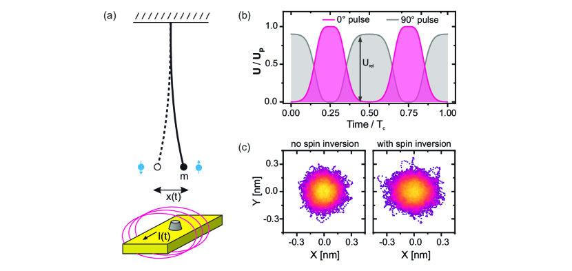
In our setup, the fundamental mode of a silicon cantilever acts as the mechanical sensor. The cantilever is positioned in the pendulum geometry above a gold microstrip fabricated on top of a thermally oxidized silicon chip. The cantilever has a resonance frequency , an effective mass , and a quality factor . For spin-mechanics experiments, a sample is attached to the tip of the cantilever and colled down to . The spin ensemble inside the sample, which is the typical subject of study in MRFM, is illustrated by a single blue spin in Fig. 1(a).
In order to manipulate the spin ensemble, amplitude- and frequency-modulated rf current pulses with a carrier frequency around are sent through the microstrip on the chip surface Grob et al. (2019). The current generates rf magnetic fields that flip spins once every pulse, see pink outlines in Fig. 1(b). With a pulse repetition rate of , the interaction of the -component of the spin ensemble with the magnetic field gradient of a nanoscale ferromagnet [Fig. 1(a)] creates a periodic force that drives the cantilever oscillation at . Stochastic spin fluctuations with lifetime slowly change and average the mean force signal to zero over long integration times . For this reason, it is usually the added oscillation variance caused by the fluctuating spin force that serves as the spin signal in MRFM Degen et al. (2007); Herzog et al. (2014). By selecting the pulse phase relative to the lock-in amplifier clock at , the phase of can be controlled; in the example shown in Fig. 1(c), the spin signal is chosen to be in the X channel. The spin force manifests as a difference between the variances in the two quadratures, . Note that the pulses at do not cause direct electrostatic driving of the cantilever mode at because they do not break the symmetry over one period .
Surprisingly, a significant imbalance between and can be observed experimentally even when the pulses are detuned from and do not excite any spins. In such a situation, one would expect that the pulses have no effect on the cantilever mode and that the phase space portrait of the thermal fluctuations remains circular as in Fig. 2(a). Instead, we clearly observe a significant imbalance in Fig. 2(b). This imbalance could be misinterpreted as a spin signal. In the past, this spurious driving was carefully avoided by heuristic pulse optimization Longenecker et al. (2012); Moores et al. (2015); Grob et al. (2019); Krass et al. (2022); Pachlatko et al. (2024). When the phase of the pulse is rotated by , the resulting variance is rotated as well, yielding in Fig. 2(c). When combining both sets of pulses, we return to a balanced distribution , see Fig. 2(d). Here, both quadratures are slightly enlarged relative to Fig. 2(a), indicating an increase in the effective cantilever mode temperature.
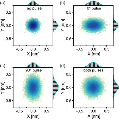
To understand the observations in Fig. 2, we need to consider two independent effects. On the one hand, current pulses dissipate energy, heating the cantilever mode irrespective of the pulse shape or phase. We assign the increase of and in Fig. 2(d) relative to Fig. 2(a) to such Joule heating. On the other hand, we observe that the squared field strength associated with the spin inversion pulses can modify the cantilever spring constant, see Fig. 3. We tentatively associate this effect with electrostatic interactions between the biased surface and random charges on the cantilever tip Héritier et al. (2021). When the field power is modulated in time with a rate close to , it causes positive and negative parametric amplification of the orthogonal oscillation quadratures Rugar and Grütter (1991); Lifshitz (2009); Eichler and Zilberberg (2023).

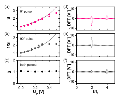
To show that parametric amplification can be used to model our experimental observations, we examine the measured squeezing factor in Fig. 4. When only the ‘’ rf pulses are applied (without inverting any spins), increases monotonically with the maximum pulse amplitude . By contrast, when only the rotated ‘’ pulses are used, the inverse increases monotonically with . Both findings are in agreement with the observations in Fig. 2. Beyond , the squeezing saturates for both pulse types. In this voltage regime, we found spurious effects in our pulse protocol that may cause further artifacts. We avoid this voltage range in our MRFM experiments and also ignore it in the following discussion.
To quantify the changes in , we plot in Fig. 4(a) and (b) the expected parametric squeezing ratio Lifshitz (2009) as solid lines, where is a heuristic factor to account for the interaction efficiency between the pulses and the cantilever displacement. This simple model accounts well for the observed increase in and , respectively, in the relevant range . When parametric amplification is applied to both quadratures simultaneously, symmetry between fluctuations in and should be restored. Indeed, in Fig. 4(c) we show that when both and are combined. This entails that pulses can be used to counter unwanted squeezing during spin detection measurements.
The origin of the parametric squeezing, and its cancellation by the combination of and pulses, can be confirmed by a Fourier analysis of the applied pulse shapes. In Fig. 4(d), we display the discrete Fourier transform (DFT) of the measured squared pulse voltage (the pulse power) for the pulse. The spectrum has a peak at , as expected from the amplitude modulation of the pulse, as depicted in Fig. 1(b). This Fourier component at is responsible for parametric amplification and squeezing of the cantilever oscillations. We obtain the same result for the pulse in Fig. 4(e). However, the sign of the component at is inverted, as expected for the DFT of a squared and phase-shifted sinusoidal signal. Finally, when both pulses are combined, the positive and negative peaks of the pulses cancel and the resulting spectrum has almost no signature near . As a consequence, no parametric squeezing effects are present.
Note that the and pulses can have different amplitude modulation functions and peak amplitudes, c.f. Fig. 1(b). As long as the -component of both pulses is equal in magnitude, the parametric squeezing is compensated. This enables significant freedom in optimizing spin inversion protocols.
In summary, we reveal that spin inversion pulses in MRFM can result in parametric squeezing of cantilever vibrations, which yields a signal that closely resembles that of a real spin force. The effect can be cancelled by combining two sets of phase-shifted pulses: the pulses are applied at a carrier frequency to invert nuclear spins within a selected Larmor frequency band, while the pulse are detuned from and do not excite spins. This method is very robust: once a suitable pulse is found, the compensation works regardless of the instantaneous cantilever frequency or the pulse amplitude scaling, which is very beneficial for scanning experiments. A disadvantage of adding the pulses is increased Joule heating, as shown in Fig. 2(d). For this reason, it is worth considering alternative methods for reducing the squeezing effect of the pulses.
With a careful calibration of the parametric interaction, the squeezing can be removed from the collected spin force data in post analysis by applying the function inverse , where the value of can be obtained from a measurement series such as shown in Fig. 4(a). With this method, no second pulse is required to cancel the resonator oscillation squeezing, and hence Joule heating is reduced. Squeezing can potentially even turn into a resource for enhancing the spin signal relative to amplifier noise, leading to an enhanced signal-to-noise ratio. However, note that the ratio between the measured spin force and force fluctuations acting on the sensor is not changed by squeezing, hence no sensitivity increase relative to the dominant thermomechanical force noise is expected.
We expect that the understanding of parametric effects related to spin driving will enable researchers to design better pulse shapes via optimal control theory Rose et al. (2018) and machine learning, thereby leading to improved spin sensing protocols. Such design rules will be crucial for establishing spin sensing protocols with mechanical sensors in the MHz regime. These are expected to improve spin sensitivity, but come with the need for much faster nuclear spin manipulations Košata et al. (2020); Eichler (2022); Haas et al. (2022); Tabatabaei et al. (2024).
Acknowledgments
We thank the operations team of the FIRST cleanroom, especially Sandro Loosli and Petra Burkard, as well as the operations team of the Binnig and Rohrer Nanotechnology Center (BRNC) at IBM Rüschlikon, especially Ute Drechsler, Richard Stutz and Dr. Diana Dávila Pineda. A. E. acknowledges financial support from Swiss National Science Foundation (SNSF) through grants 200021_200412 and CRSII5_206008/1.
The authors have no conflicts to disclose.
The data that support the findings of this study are available from the corresponding author upon reasonable request.
References
- Rabl et al. (2010) P. Rabl, S. J. Kolkowitz, F. Koppens, J. Harris, P. Zoller, and M. D. Lukin, Nature Physics 6, 602 (2010).
- Sidles (1991) J. A. Sidles, Applied Physics Letters 58, 2854 (1991).
- Sidles et al. (1992) J. A. Sidles, J. L. Garbini, and G. P. Drobny, Review of Scientific Instruments 63, 3881 (1992).
- Rugar et al. (1992) D. Rugar, C. Yannoni, and J. Sidles, Nature 360, 563 (1992).
- Poggio and Degen (2010) M. Poggio and C. L. Degen, Nanotechnology 21, 342001 (2010).
- Degen et al. (2009) C. Degen, M. Poggio, H. Mamin, C. Rettner, and D. Rugar, Proceedings of the National Academy of Sciences 106, 1313 (2009).
- Grob et al. (2019) U. Grob, M. D. Krass, M. Héritier, R. Pachlatko, J. Rhensius, J. Košata, B. A. Moores, H. Takahashi, A. Eichler, and C. L. Degen, Nano Letters 19, 7935 (2019).
- Krass et al. (2022) M.-D. Krass, N. Prumbaum, R. Pachlatko, U. Grob, H. Takahashi, Y. Yamauchi, C. L. Degen, and A. Eichler, Phys. Rev. Appl. 18, 034052 (2022).
- Tsaturyan et al. (2017) Y. Tsaturyan, A. Barg, E. S. Polzik, and A. Schliesser, Nature Nanotechnology 12, 776 (2017).
- Reetz et al. (2019) C. Reetz, R. Fischer, G. Assumpção, D. McNally, P. Burns, J. Sankey, and C. Regal, Physical Review Applied 12, 044027 (2019).
- Ghadimi et al. (2018) A. H. Ghadimi, S. A. Fedorov, N. J. Engelsen, M. J. Bereyhi, R. Schilling, D. J. Wilson, and T. J. Kippenberg, Science 360, 764 (2018).
- Gisler et al. (2022) T. Gisler, M. Helal, D. Sabonis, U. Grob, M. Héritier, C. L. Degen, A. H. Ghadimi, and A. Eichler, Phys. Rev. Lett. 129, 104301 (2022).
- Bereyhi et al. (2022) M. J. Bereyhi, A. Arabmoheghi, A. Beccari, S. A. Fedorov, G. Huang, T. J. Kippenberg, and N. J. Engelsen, Phys. Rev. X 12, 021036 (2022).
- Shin et al. (2022) D. Shin, A. Cupertino, M. H. J. de Jong, P. G. Steeneken, M. A. Bessa, and R. A. Norte, Advanced Materials 34, 2106248 (2022).
- Eichler (2022) A. Eichler, Materials for Quantum Technology 2, 043001 (2022).
- Nichol et al. (2013) J. M. Nichol, T. R. Naibert, E. R. Hemesath, L. J. Lauhon, and R. Budakian, Phys. Rev. X 3, 031016 (2013).
- Mamin et al. (2007) H. Mamin, M. Poggio, C. Degen, and D. Rugar, Nature nanotechnology 2, 301 (2007).
- Vinante et al. (2011) A. Vinante, G. Wijts, O. Usenko, L. Schinkelshoek, and T. Oosterkamp, Nature communications 2, 572 (2011).
- Košata et al. (2020) J. Košata, O. Zilberberg, C. L. Degen, R. Chitra, and A. Eichler, Phys. Rev. Applied 14, 014042 (2020).
- Degen et al. (2007) C. L. Degen, M. Poggio, H. J. Mamin, and D. Rugar, Phys. Rev. Lett. 99, 250601 (2007).
- Degen et al. (2008) C. L. Degen, M. Poggio, H. J. Mamin, and D. Rugar, Phys. Rev. Lett. 100, 137601 (2008).
- Slichter (2013) C. P. Slichter, Principles of magnetic resonance, Vol. 1 (Springer Science & Business Media, 2013).
- Herzog et al. (2014) B. Herzog, D. Cadeddu, F. Xue, P. Peddibhotla, and M. Poggio, Applied Physics Letters 105 (2014).
- Longenecker et al. (2012) J. G. Longenecker, H. Mamin, A. W. Senko, L. Chen, C. T. Rettner, D. Rugar, and J. A. Marohn, ACS nano 6, 9637 (2012).
- Moores et al. (2015) B. Moores, A. Eichler, Y. Tao, H. Takahashi, P. Navaretti, and C. L. Degen, Applied Physics Letters 106 (2015).
- Pachlatko et al. (2024) R. Pachlatko, N. Prumbaum, M.-D. Krass, U. Grob, C. L. Degen, and A. Eichler, Nano Letters 24, 2081 (2024).
- Héritier et al. (2021) M. Héritier, R. Pachlatko, Y. Tao, J. M. Abendroth, C. L. Degen, and A. Eichler, Physical Review Letters 127, 216101 (2021).
- Rugar and Grütter (1991) D. Rugar and P. Grütter, Phys. Rev. Lett. 67, 699 (1991).
- Lifshitz (2009) M. C. Lifshitz, R. Cross, “Nonlinear dynamics of nanomechanical and micromechanical resonators,” in Reviews of Nonlinear Dynamics and Complexity (Wiley-VCH, 2009) pp. 1–52.
- Eichler and Zilberberg (2023) A. Eichler and O. Zilberberg, Classical and Quantum Parametric Phenomena (Oxford University Press, 2023).
- Rose et al. (2018) W. Rose, H. Haas, A. Q. Chen, N. Jeon, L. J. Lauhon, D. G. Cory, and R. Budakian, Physical Review X 8, 011030 (2018).
- Haas et al. (2022) H. Haas, S. Tabatabaei, W. Rose, P. Sahafi, M. Piscitelli, A. Jordan, P. Priyadarsi, N. Singh, B. Yager, P. J. Poole, et al., Proceedings of the National Academy of Sciences 119, e2209213119 (2022).
- Tabatabaei et al. (2024) S. Tabatabaei, P. Priyadarsi, N. Singh, P. Sahafi, D. Tay, A. Jordan, and R. Budakian, arXiv preprint arXiv:2402.16283 (2024).