Faster Lattice Basis Computation - The Generalization
of the Euclidean Algorithm

Abstract

The Euclidean algorithm the oldest algorithms known to mankind. Given two integral numbers $a_{1}$ and $a_{2}$, it computes the greatest common divisor (gcd) of $a_{1}$ and $a_{2}$ in a very elegant way. From a lattice perspective, it computes a basis of the sum of two one-dimensional lattices $a_{1}\mathbb{Z}$ and $a_{2}\mathbb{Z}$ as $\gcd(a_{1},a_{2})\mathbb{Z}=a_{1}\mathbb{Z}+a_{2}\mathbb{Z}$. In this paper, we show that the classical Euclidean algorithm can be adapted in a very natural way to compute a basis of a general lattice $\operatorname{\mathcal{L}}(A_{1},\ldots,A_{n})$ given vectors $A_{1},\ldots,A_{n}\in\mathbb{Z}^{d}$ with $n>\mathrm{rank}(a_{1},\ldots,a_{d})$. Similar to the Euclidean algorithm, our algorithm is very easy to describe and implement and can be written within 12 lines of pseudocode.

Our generalized version of the Euclidean algorithm allows for several degrees of freedom in the pivoting process. Hence, in a second step, we show that this freedom can be exploited to make the algorithm perform more efficiently. As our main result, we obtain an algorithm to compute a lattice basis for given vectors $A_{1},\ldots,A_{n}\in\mathbb{Z}^{d}$ in time (counting bit operations) $LS+\tilde{O}((n-d)d^{2}\cdot\log(||A||)$, where $LS$ is the time required to obtain the exact fractional solution of a certain system of linear equalities. The analysis of the running time of our algorithms relies on fundamental statements on the fractionality of solutions of linear systems of equations.

So far, the fastest algorithm for lattice basis computation was due to Storjohann and Labhan [SL96] having a running time of $\tilde{O}(nd^{\omega}\log\left\lVert A\right\rVert)$. We can improve upon their running time by guaranteeing a running time of $\tilde{O}(\max\{n-d,d\}d^{\omega(2)-1}\log\left\lVert A\right\rVert)$ for our algorithm. For current values of $\omega$ and $\omega(2)$, our algorithm thus improves the running time by a factor of at least $d^{0.12}$ (since $n>d$) providing the first general runtime improvement in nearly 30 years. In the cases of either few additional vectors, e.g. $n-d\in d^{o(1)}$, or a very large number of additional vectors, e.g. $n-d\in\Omega(d^{k})$ and $k>1$, the run time improves even further in comparison.

1 Introduction

Given two integral numbers $a_{1}$ and $a_{2}$, the Euclidean algorithm computes the greatest common divisor (gcd) of $a_{1}$ and $a_{2}$ in a very elegant way. Starting with $s=a_{1}$ and $t=a_{2}$, a residue $r$ is being computed by setting

$$r=\min_{x\in\mathbb{Z}}\{r\in\mathbb{Z}\mid sx+r=t\}=\min\{t\pmod{s},|(t\pmod{s})-s|\}.$$

This procedure is continued iteratively with $s=t$ and $t=r$ until $r$ equals $0$. Since $r\leq\lfloor t/2\rfloor$ the algorithm terminates after at most $\log(\min\{a_{1},a_{2}\})$ many iterations.

An alternative interpretation of the gcd or the Euclidean algorithm is the following: Consider all integers that are divisible by $a_{1}$ or respectively $a_{2}$, which is the set $a_{1}\mathbb{Z}$ or respectively the set $a_{2}\mathbb{Z}$. Consider their sum (i.e. Minkowski sum)

$$A=a_{1}\mathbb{Z}+a_{2}\mathbb{Z}=\{a+b\mid a\in a_{1}\mathbb{Z},b\in a_{2}\mathbb{Z}\}.$$

It is easy to see that the set $A$ can be generated by a single element, which is the gcd of $a_{1}$ and $a_{2}$, i.e.

$$a_{1}\mathbb{Z}+a_{2}\mathbb{Z}=gcd(a_{1},a_{2})\mathbb{Z}.$$

Furthermore, the set $\mathcal{L}=a_{1}\mathbb{Z}+a_{2}\mathbb{Z}$ is closed under addition, subtraction and scalar multiplication, which is why all values for $s,t$ and $r$, as defined above in the Euclidean algorithm, belong to $\mathcal{L}$. In the end, the smallest non-zero element for $r$ obtained by the algorithm generates $\mathcal{L}$ and hence $\mathcal{L}=r\mathbb{Z}=gcd(a_{1},a_{2})\mathbb{Z}$.

This interpretation does not only allow for an easy correctness proof of the Euclidean algorithm, it also allows for a generalization of the algorithm into higher dimensions. For this, we consider vectors $A_{1},\ldots,A_{n}\in\mathbb{Z}^{d}$ with $n>d$ and the set of points in space generated by sums of integral multiples of the given vectors, i.e.

$$\mathcal{L}=A_{1}\mathbb{Z}+\ldots A_{n}\mathbb{Z}.$$

The set $\mathcal{L}$ is called a lattice and is generally defined for a given matrix $A$ with column vectors $A_{1},\ldots,A_{n}$ by

$$\mathcal{L}(A)=\{\sum_{i=1}^{n}\lambda_{i}A_{i}\mid\lambda_{i}\in\mathbb{Z}\}.$$

One of the most basic facts from lattice theory is that every lattice $\mathcal{L}$ has a basis $B$ such that $\mathcal{L}(B)=\mathcal{L}(A)$, where $B$ is a square matrix. Note that the set $a_{1}\mathbb{Z}+a_{2}\mathbb{Z}$ is a one-dimensional lattice and in this sense the Euclidean algorithm simply computes a basis of the one-dimensional lattice with $gcd(a_{1},a_{2})\mathbb{Z}=a_{1}\mathbb{Z}+a_{2}\mathbb{Z}$.

Hence, morally, a multidimensional version of the Euclidean algorithm should compute for a given matrix $A=(A_{1},\ldots,A_{n})$ a basis $B\in\mathbb{Z}^{d\times d}$ such that

$$\mathcal{L}(B)=\mathcal{L}(A).$$

The problem of computing a basis for the lattice $\operatorname{\mathcal{L}}(A)$ is called lattice basis computation. In this paper, we show that the classical Euclidean algorithm can be generalized in a very natural way to do just that. Using this approach, we improve upon the running time of existing algorithms for lattice basis computation.

1.1 Lattice Basis computation

The first property of a lattice that is typically taught in a lattice theory lecture is the fact that each lattice has a basis. Computing a basis of a lattice is one of the most basic algorithmic problems in lattice theory. Often it is required as a subroutine by other algorithms [Ajt96, BP87, GPV08, MG02, Poh87]. There are mainly two methods on how a basis of a lattice can be computed. The most common approaches rely on either a variant of the LLL-algorithm or on computing the Hermite normal form (HNF), where the fastest algorithms all rely on the HNF. Considering these approaches however, one encounters two major problems. First, the entries of the computed basis can be as large as the determinant and therefore exponential in the dimension. Secondly and even worse, intermediate numbers on the computation might even be exponential in their bit representation. This effect is called intermediate coefficient swell. Due to this problem, it is actually not easy to show that a lattice basis can be computed in polynomial time. Kannan und Buchem [KB79] were the first ones to show that the intermediate coefficient swell can be avoided when computing the HNF and hence a lattice basis can actually be computed in polynomial time. The running time of their algorithm was later improved by Chou and Collins[CC82] and Iliopoulos [Ili89].

Recent and the most efficient algorithms for lattice basis computation all rely on computing the HNF, with the most efficient one being the algorithm by Storjohann and Labahn [SL96]. Given a full rank matrix $A\in\mathbb{Z}^{d\times n}$ the HNF can be computed by using only $\operatorname{\tilde{O}}(nd^{\omega}\cdot\log\left\lVert A\right\rVert)$ many bit operations, where $\omega$ denotes the exponent for matrix multiplication and is currently $\omega\leq 2.371552$ [WXXZ24]. The algorithm by Labahn and Storjohann [SL96] improves upon a long series of papers [KB79, CC82, Ili89] and has not been improved since its publication in 1996. Only in the special case that $n-d=1$, Li and Storjohann [LS22] manage to obtain a running time of $\operatorname{\tilde{O}}(d^{\omega}\cdot\log\left\lVert A\right\rVert)$ which essentially matches matrix multiplication time.

Other recent paper considering lattice basis computation focus on properties other than improving the running time. There are several algorithms that preserve orthogonality from the original matrix, e. g. $\left\lVert B^{*}\right\rVert\leq\left\lVert A^{*}\right\rVert$, or improve on the $\ell_{\infty}$ norm of the resulting matrix [NSV11, NS16], or both [HPS11, LN19, CN97, MG02]. Except for the HNF based basis algorithm by Lin and Nguyen [LN19], all of the above algorithms have a significantly higher time complexity compared to Labahn’s and Storjohann’s HNF algorithm. The algorithm by Lin and Nguyen use existing HNF algorithms and apply a separate coefficient reduction algorithm resulting in a basis with $\ell_{\infty}$ norm bounded by $d\left\lVert A\right\rVert$.

1.2 Our Contribution

In this paper we develop a fundamentally new approach for lattice basis computation given a matrix $A$ with column vectors $A_{1},\ldots,A_{n}\in\mathbb{Z}^{d}$. Our approach does not rely on any normal form of a matrix or the LLL algorithm. Instead, we show a direct way to generalize the classical Euclidean algorithm to higher dimensions. After a thorough literature investigation and talking to many experts in the area, we were surprised to find out that this approach actually seems to be new.

Our approach does not suffer from intermediate coefficient growth and hence gives an easy way to show that a lattice basis can be computed in polynomial time.

Similar to the Euclidean algorithm, our algorithm chooses an initial basis $B$ from the given vectors and updates the basis according to a remainder operation and then exchanges a vector by this remainder. In every iteration, the determinant of $B$ decreases by a factor of at least $1/2$ and hence the algorithm terminates after at most $\log\det(B)$ many iterations. Similar to the Euclidean algorithm, our algorithms can be easily described and implemented.

In Section 3, we modify our previously developed generalization of the Euclidean algorithm in order to make it more efficient. We exploit the freedom in the pivotization and also combine several iterations at once to optimize its running time. Our main result is an algorithm which requires

$$LS(d,n-d,\left\lVert A\right\rVert)+\tilde{O}((n-d)d^{2}\cdot\log(\left\lVert A\right\rVert)),$$

many bit operations, where $LS(d,n-d,\left\lVert A\right\rVert)$ is the time required to obtain an exact fractional solution matrix $X\in\mathbb{Z}^{d\times(n-d)}$ to a linear system $BX=C$, with matrix $B\in\mathbb{Z}^{d\times d}$ and matrix $C\in\mathbb{Z}^{d\times(n-d)}$ with $\left\lVert B\right\rVert,\left\lVert C\right\rVert\leq\left\lVert A\right\rVert$. Based on the work of  [BLS19], we argue in Section 3.4 that the term $LS(d,n-d,\left\lVert A\right\rVert)$, being the bottleneck of the algorithm, can be bounded by

$$\tilde{O}(\max\{n-d,d^{k}\}d^{\omega(k+1)-k}\log\left\lVert A\right\rVert)$$

for every $k\geq 0$, where $\omega(k)$ is the matrix multiplication exponent of an $n\times n^{k}$ matrix by an $n^{k}\times n$ matrix (see [Gal24]). Setting $k=1$, we obtain a running time of $\tilde{O}(\max\{n-d,d\}d^{\omega(2)-1}\log\left\lVert A\right\rVert)$, with $\omega(2)\approx 3.250563$. This shows that we can improve upon the algorithm by Storjohann and Labhan [SL96] in any case at least by a factor of roughly $d^{0.12}$ and therefore obtain the first general improvement to this fundamental problem in nearly 30 years. Any future improvement that one can achieve in the computation of exact fractional solution to linear systems would directly translate to an improvement of our algorithm.

Setting $k=0$ yields a running time of $\tilde{O}((n-d)d^{\omega}\log\left\lVert A\right\rVert)$ for our algorithm. Hence, this improves upon the algorithm by Storjohann and Labhan [SL96] in the case that $n-d\in o(d)$. In the case that $n-d\in O(1)$ by this we match the running time of the algorithm by Li and Storjohann [LS22]. Note however, that the algorithm by Li and Storjohann can not be iterated to obtain an running time of the same running time for $n-d\in\Omega(1)$. This is due to a coefficient blowup in the output matrix.

Besides the new algorithmic approach, one main tool that we develop is a structural statement on the fractionality of solutions of linear systems. Note that when considering bit operations instead of only counting arithmetic operations, one has to pay attention to the bit length of the respective numbers. When operating with precise fractional solutions to linear systems, one can typically only bound the bit length of the numbers by $\tilde{O}(d\log(\left\lVert A\right\rVert))$. Hence, we would obtain this term as an additional factor when one is adding or multiplying these numbers. In order to deal with this issue and obtain a better running time, we prove in Section 3.1 a fundamental structural statement regarding the fractionality (i.e. the size of the denominator) of solutions to linear systems of equations. Essentially, we show that the fractionality of the solutions is only large if there are few integral points contained in a subspace of $\operatorname{\mathcal{L}}(B)$ and vice versa. This structural statement can then be used in the runtime analysis of our algorithm as it iterates over the integral points in the respective subspace.

In terms of coefficient growth of the output basis matrix we can show that our algorithm always return a solution matrix $S$ such that $\left\lVert S\right\rVert\leq d\left\lVert A\right\rVert$.

2 A Multi-Dimensional Generalization of the Euclidean Algorithm

In this section and throughout the paper, we assume that $rank(A)=d$ and therefore the lattice $\operatorname{\mathcal{L}}(A)$ is full dimensional. However, our algorithms can be applied in a similar way if $rank(A)<d$.

Preliminaries

Consider a (not necessarily full) dimensional lattice $\operatorname{\mathcal{L}}(B)$ for a given basis $B\in\mathbb{Z}^{d\times j}$ with $j\leq d$. An important notion that we need is the so called fundamental parallelepiped

$$\Pi(B)=\{Bx\mid x\in[0,1)^{j}\}$$

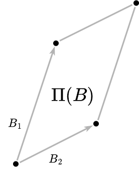
Figure 1: The parallelepiped of $B=(B_{1}B_{2})$.

see also Figure 1. Let $V$ be the space generated by the columns in $B$. As each point $a\in\mathbb{R}^{d}$ can be written as

$$a=B\lfloor x\rfloor+B\{x\},$$

it is easy to see that the space $V$ can be partitioned into parallelepipeds. Here, $\lfloor x\rfloor$ denotes the vector, where each component $x_{i}$ is rounded down and $\{x\}=x-\lfloor x\rfloor$ is the vector with the respective fractional entries $x_{i}\in[0,1)$. In fact, the notion of $\Pi(B)$ allows us to define a multi-dimensional modulo operation by mapping any point $a\in V\cap\mathbb{Z}^{d}$ to the respective residue vector in the parallelepiped $\Pi(B)$, i.e.

$$a\pmod{\Pi(B)}:=B\{B^{-1}a\}\in\Pi(B).$$

Furthermore, for $a\in\mathbb{Z}^{d}$, we denote with $\lfloor z\rceil$ the next integer from $a$, which is $\lfloor a+1/2\rfloor$. When we use these notations on a vector $a\in\mathbb{Z}^{d}$, the operation is performed entry-wise.

Note that in the case that $B\in\mathbb{Z}^{d\times d}$ the parallelepiped $\Pi(B)$ has the nice property, that its volume as well as the number of contained integer points is exactly $\det(B)$, i.e.

$$vol(\Pi(B))=|\Pi(B)\cap\mathbb{Z}^{n}|=\det(B).$$

In the following we will denote by $A_{i}$ the $i-th$ column vector of a matrix $A$. In the case that $a\in\mathbb{Z}^{d}$ is a vector we will denote by $a_{i}$ the $i$-th entry of $a$. To simplify the notation, we denote by $\det(B)$ the absolute value of the determinant of $B$ and by $\left\lVert B\right\rVert$ of a matrix $B$ or a vector $B$, we denote the respective infinity norm, meaning the largest entry of $B$.

In our algorithm, we will change our basis over time by exchanging column vectors. We denote the exchange of column $i$ of a matrix $B$ with a vector $v$ by $B\setminus B_{i}\cup v$. The notation $B\cup v$ for a matrix $B$ and a vector $v$ of suitable dimension denotes the matrix, where $v$ is added as another column to matrix $B$. Similarly, the notation $B\cup S$ for a matrix $B$ and a set of vectors $S$ (with suitable dimension) adds the vectors of $S$ as new columns to matrix $B$. While the order of added columns is ambiguous, we will use this operation only in cases where the order of column vectors does not matter.

Our algorithms use three different subroutines from the literature. First, in order to compute a submatrix $B$ of $A$ of maximum rank, we use the following theorem.

Lemma 1 ([LS22]).

Let $A\in\mathbb{Z}^{\tilde{d}\times\tilde{n}}$ have full column rank. There exists an algorithm that finds indices $i_{1},\ldots,i_{\tilde{d}}$ such that $A_{i_{1}},\ldots,A_{i_{\tilde{d}}}$ are linearly independent using $\operatorname{\tilde{O}}(\tilde{n}\tilde{d}^{\omega-1}\cdot\log\left\lVert A\right\rVert)$ bit operations.

As a second subroutine which is required in Section 3 to compute the greatest common divisor of two numbers $a_{1},a_{2}\leq a$, we use the algorithm by Schönhage [Sch71] which requires $\tilde{O}(\log a)$ many bit operations. Note, that the bit complexity of the classical Euclidean algorithm is actually $\tilde{O}(\log^{2}a)$ as in each iteration of the algorithm, the algorithm operates with numbers having $O(\log a)$ bits.

As a third subroutine, we require an algorithm to solve linear systems of equations of the form $Bx=c$. Due to its equivalence to matrix multiplication this can be done in time $O(d^{\omega})$ time counting only arithmetic operations. However, since we use the more precise analysis of bit operations, we use the algorithm by Birmpilis, Labahn, and Storjohann [BLS19] who developed an algorithm analyzing the bit complexity of linear system solving. Their algorithm requires $\tilde{O}(d^{\omega}\cdot\log\left\lVert A\right\rVert)$ many bit operations. We slightly modify their algorithm in section 3.4 to obtain an efficient algorithm solving $BX=C$ for some matrix $C$ in order to compute a solution matrix $X$.

2.1 The Algorithm

Given two numbers, the classical Euclidean algorithm, essentially consists of two operations. First, a modulo operation computes the modulo of the larger number and the smaller number. Second, an exchange operation discards the larger number and adds the remainder instead. The algorithm continues with the smaller number and the remainder.

Given vectors $A=\{A_{1},\ldots,A_{d+1}\}\subset\mathbb{Z}^{d}$, our generalized algorithm performs a multi-dimensional version of modulo and exchange operations of columns with the objective to compute a basis $B\in\mathbb{Z}^{d\times d}$ with $\operatorname{\mathcal{L}}(B)=\operatorname{\mathcal{L}}(A)$. First, we choose $d$ linearly independent vectors from $A$ which form a non-singular matrix $B$. The lattice $\operatorname{\mathcal{L}}(B)$ is a sub-lattice of $\operatorname{\mathcal{L}}(A)$. Having this sub-basis, we can perform a division with residue in the lattice $\operatorname{\mathcal{L}}(B)$. Hence, the remaining vector $a\in A\setminus B$ can be represented as

$$a=B\lfloor B^{-1}a\rfloor+r,$$

where $r$ is the remainder $a\pmod{\Pi(B)}$, see also subfigure 2a.

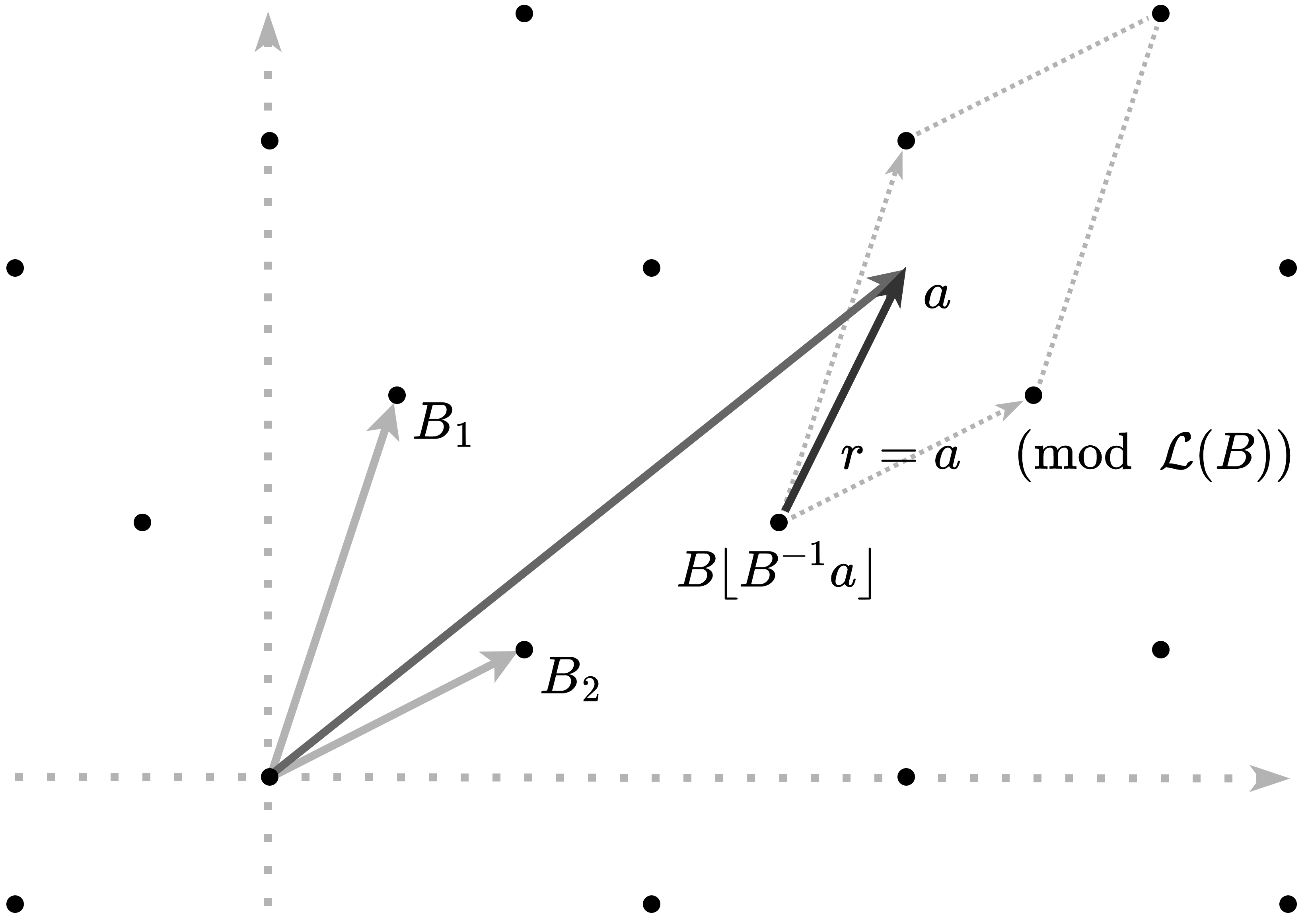
(a) The modulo operation in dimension $2$.

(b) Exchange of a basis vector and the parallelopipeds for $B_{1}$ and $B_{2}$ (solid), $B_{2}$ and $r$ (dotted), and $B_{2}$ and $r^{\prime}$ (dashed).

Figure 2: The modulo operation with respect to a lattice and the exchange operation depending on $\lfloor x_{1}\rceil$.

In dimension $d=1$ this is just the classical division with residue and the corresponding modulo operation, i. e. $a=b\cdot\lfloor a/b\rfloor+r$.

Having the residue vector $r$ at hand, the exchange step of our generalized version of the Euclidean algorithm exchanges a column vector of $B$ with the residue vector $r$. In dimension $>1$, we have the choice on which column vector to discard from $B$. The choice we make is based on the solution $x\in\mathbb{Q}^{d}$ of the linear system $Bx=a$.

• Case 1: $x\in\mathbb{Z}^{d}$. In the case that the solution $x$ is integral, we know that $a\in\operatorname{\mathcal{L}}(B)$ and hence $\operatorname{\mathcal{L}}(B\cup a)=\operatorname{\mathcal{L}}(B)$. Our algorithm terminates.

• Case 2: There is a fractional component $\ell$ of $x$. In this case, our algorithm exchanges $B_{i}$ with $r$, i. e. $B^{\prime}=B\setminus B_{\ell}\cup r$.

The algorithm iterates this procedure with basis $B^{\prime}$ and vector $a=B_{\ell}$ until Case 1 is achieved.

[3.5em]3.5em

Two questions arise: Why is this algorithm correct and why does it terminate?

Termination:
The progress in step 2 can be measured in terms of the determinant. For $x$ with $Bx=a$ the exchange step in case 2 swaps $B_{i}$ with $r=B\{x\}$ and $\{x_{i}\}\neq 0$ to obtain the new basis $B^{\prime}$. By Cramer’s rule we have that $\{x_{\ell}\}=\frac{\det B^{\prime}}{\det B}$ and hence the determinant decreases by a factor of $\{x_{\ell}\}<1$. The algorithm eventually terminates since $\det(\operatorname{\mathcal{L}}(A))\geq 1$ and all involved determinants are integral since the corresponding matrices are integral. A trivial upper bound for the number of iterations is the determinant of the initial basis.

Correctness:
Correctness of the algorithm follows by the observation that $\operatorname{\mathcal{L}}(B\cup a)=\operatorname{\mathcal{L}}(B\cup r)$. To see this, it is sufficient to prove $a\in\operatorname{\mathcal{L}}(B\cup r)$ and $r\in\operatorname{\mathcal{L}}(B\cup a)$. By the definition of $r$ we get that $a=Bx=B\lfloor x\rfloor+B\{x\}=B\lfloor x\rfloor+r$. Hence, $a$ and $r$ are integral combinations of vectors from $B\cup r$ and $B\cup a$, respectively, and hence $\operatorname{\mathcal{L}}(B\cup a)=\operatorname{\mathcal{L}}(B\cup r)$.

The multiplicative improvement of the determinant in step 2 can be very close to $1$, i. e. $\frac{\det(B)-1}{\det(B)}$. In the classical Euclidean algorithm a step considers the remainder $r$ for $a=b\lfloor a/b\rfloor+r$. The variant described in section 1 considers an $r^{\prime}$ for $a=b\lfloor a/b\rceil+r^{\prime}$. Taking the next integer instead of rounding down ensures that in every step the remainder in absolute value is at most half of the size of $b$. Our generalized Euclidean algorithm uses a modified modulo operation that does just that in a higher dimension. In our case, this modification ensures that the absolute value of the determinant decreases by a multiplicative factor of at most $1/2$ in every step as we explain below. The number of steps is thus bounded by $\log\det(B)$. The generalization to higher dimensions chooses $i$ such that $x_{i}$ is fractional and rounds it to the next integer $\lfloor x_{i}\rceil$ while the other entries of $x$ are again rounded $\lfloor x_{j}\rfloor$ for $j\neq i$. Formally, this modulo variant is defined as

$$a\ \ (\bmod^{\prime}\ \Pi(B)):=r^{\prime}:=a-(\sum_{j\neq i}B_{j}\lfloor x_{j}\rfloor+B_{i}\lfloor x_{i}\rceil)$$

for $Bx=a$ and some $i$ such that $\{x_{i}\}\neq 0$. By Cramer’s rule we get that the determinant decreases by a multiplicative value of at least $1/2$ in every iteration since $\frac{1}{2}\leq\left\lvert x_{i}-\lfloor x_{i}\rceil\right\rvert=\left\lvert\frac{\det B^{\prime}}{\det B}\right\rvert$.

In subfigure 2b the resulting basis for exchanging $B_{1}$ with $r=a\ \ (\bmod\ \Pi(B))$ and with $r^{\prime}=a\ \ (\bmod^{\prime}\ \Pi(B))$ shows that in both cases the volume of the parallelepiped decreases, which is equal to the determinant of the lattice. In Figure 3, an example of our algorithm is shown.

(a) Application of our algorithm, $r^{\prime}$ is the first remainder.

(b) Vectors $r^{\prime}$ and $B_{1}$ were exchanged and $r^{\prime\prime}$ denotes the second remainder.

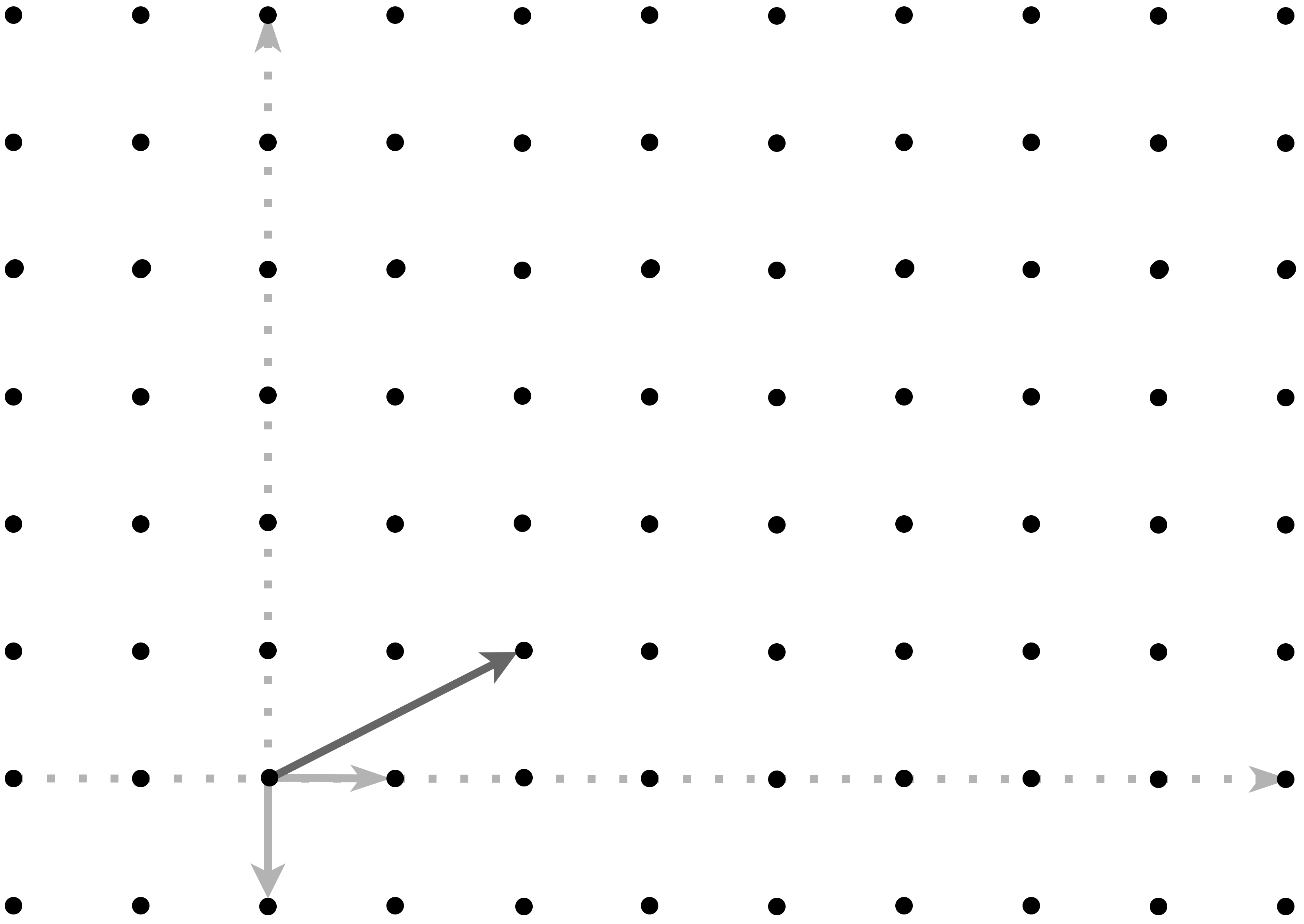
(c) Vectors $r^{\prime}$ and $B_{2}$ were exchanged. $B_{2}$ is in the lattice and the algorithm terminates.

Figure 3: An application of the algorithm.

2.2 Formal Description of the Algorithm

In the following, we state the previously described algorithm formally.

Algorithm 1 Generalized Euclidean Algorithm (Basic Algorithm)

1 Input: A matrix $A=\left(A_{1},\ldots,A_{n}\right)\in\mathbb{Z}^{d\times n}$

2 find independent vectors $B:=\left(B_{1},\ldots,B_{d}\right)$ with $B_{i}\in\{A_{1},\ldots,A_{n}\}$

3 $C$ $\leftarrow$ $\{A_{1},\ldots,A_{n}\}\setminus\{B_{1},\ldots,B_{d}\}$

4 while $C\neq\emptyset$ do

5      choose any $c\in C$

6      solve $Bx=c$

7      if $x$ is integral then

8          $C$ $\leftarrow$ $C\setminus\{c\}$

9      else

10          choose index $\ell\leq d$ with $\{x_{\ell}\}\neq 0$

11          $C$ $\leftarrow$ $C\setminus\{c\}\cup\{B_{\ell}\}$

12          $B_{\ell}$ $\leftarrow$ $c-(B_{\ell}\lfloor x_{\ell}\rceil+\sum_{j\neq\ell}B_{j}\lfloor x_{j}\rfloor)$      

13 return $B$

Theorem 1.

Algorithm 1 computes a basis for the lattice $\mathcal{L}(A)$.

Proof.

Let us consider the following invariant.

Claim. In every iteration $\mathcal{L}(A)=\mathcal{L}(B\cup C)$.

By the definition of $B$ and $C$ the claim holds in line 2. We need to prove that removing $c$ from $C$ in line $7$ and altering $B$ and $C$ in lines 9-11 do not change the generated lattice. In line 7 we found $c$ is an integral combination of vectors in $B$. Thus, every lattice point can be represented without the use of $c$ and $c$ can be removed without altering the generated lattice. In lines 9 and 10 a vector $c$ is removed from $B\cup C$ and instead a vector $c^{\prime}=c-(\sum_{j\neq i}B_{j}\lfloor x_{j}\rfloor+B_{i}\lfloor x_{i}\rceil)$ is added. By the definition of $c^{\prime}$, the removed vector $c$ is an integral combination of vectors $c^{\prime},B_{1},\ldots,B_{n}$ and $c^{\prime}$ is an integral combination of vectors $c,B_{1},\ldots,B_{n}$. Using the same argument as above, this does not change the generated lattice.

The algorithm terminates when $C=\emptyset$. In this case $B$ is a basis of $\mathcal{L}(A)$, since by the invariant we have that $\mathcal{L}(B)=\mathcal{L}(B\cup C)=\mathcal{L}(A)$.

∎

The following observation holds as in each iteration the coefficient for the newly added row $B_{\ell}$ in l.11 equals $x_{\ell}-\lceil x_{\ell}\rfloor$ and hence in absolute value is bounded by $1/2$. By Cramer’s rule, this implies that $\frac{\det B^{\prime}}{\det B}\leq\frac{1}{2}$, where $B^{\prime}$ is the new matrix being defined by interchanging the $\ell$-th column in l.11. Hence, $\det(B^{\prime})\leq\frac{1}{2}\det(B)$ which implies the following observation.

Observation 2.1.

Algorithm 1 terminates after at most $\log\det(B)$ exchange steps, where $B$ is the matrix defined in l.1 of the algorithm.

Note for the running time of the algorithm that in each iteration the algorithm solves a linear system $Bx=c$ as its main operation. Therefore, we obtain a running time of

$$LS\cdot(\log(\det B)+(n-d)),$$

where $LS$ is the time required to solve the linear system $Bx=c$. Note however, that the coefficient in $B$ might grow over each iteration. Since the new vector is contained in $\Pi(B)$ this growth can be bounded by $d\left\lVert B\right\rVert$. Hence, the resulting matrix at the end of Algorithm 1 has entries of size at most $d^{\log(\det B)}\cdot\left\lVert B\right\rVert$.

Using the Hadamard bound $\det(B)\leq d\left\lVert B\right\rVert^{d}$ and using that $LS$ can be bounded by $\tilde{O}(d^{\omega}\cdot\log\left\lVert B\right\rVert)$ for some matrix $B\in\mathbb{Z}^{d\times d}$ [BLS19], we obtain that Algorithm 1 requires at most

$$\tilde{O}(d^{\omega+1}\log^{2}(\left\lVert A\right\rVert)\cdot(d\log(\left\lVert A\right\rVert)+(n-d)))\leq\tilde{O}(nd^{\omega+1}\cdot\log^{3}(\left\lVert A\right\rVert))$$

many bit operations as a first naive upper bound for the running time of Algorithm 1. We improve upon the running time as well as the size of the entries of the output matrix in the following section.

Note however, that Algorithm 1 does not necessarily require an exact fractional solution in l.5. It is sufficient to decide if an index of the fractional solution $x$ is in indeed fractional and the first fractional bit in order to decide on how to round. This makes an implementation of the algorithm very easy as an out of the box linear system solver can be used.

In an older version [KR23] of the paper we described methods and data structures on how Algorithm 1 can be modified to be more efficient.

3 Speeding Up the Generalized Euclidean Algorithm

In the generalized setting of the Euclidean algorithm as defined in the previous section, we have several degrees of freedom. First, in each iteration, we may choose an arbitrary vector $c\in C$. Secondly, we may choose any arbitrary index $i$ with $\{x_{i}\}$ being fractional to pivot and iterate the algorithm. We can use this freedom to optimize two things:

• the running time of the algorithm and

• the quality of the solution, i.e. the size of the matrix entries in the output solution.

In the following, we study one specific rule of pivotization which allows us to update the solution space very efficiently. Moreover, it allows us to apply the Euclidean algorithm, or respectively Schönhage’s algorithm [Sch71], as a subroutine. The main idea of the following Algorithm is to pivot always the same index until it is integral for all $c\in C$. Proceeding this way allows us to update the solution very efficiently by applying the one-dimensional classical Euclidean algorithm. In the next iteration, the algorithm continues with one of the remaining fractional indices.

Consider a basis $B\in\mathbb{Z}^{d\times d}$, and a set of vectors $C\in\mathbb{Z}^{d\times(n-d)}$ which need to be merged into the basis. Let $X_{c}\in\mathbb{Q}^{d}$ with $BX_{c}=c$ be the solution vector for each $c\in C$. For a fixed index $\ell\leq d$, every entry equals $(X_{c})_{\ell}=\frac{t_{c}}{t}$ for some numbers $t_{c}\in\mathbb{Z}$ which we call the translate of vector $c$ and some $t\in\mathbb{Z}$ with $t\leq\det(B)$. Intuitively, the translate $t_{c}$ for a vector denotes the distance between vector $c\in C$ and the subspace $V_{\ell}$ which is generated by the columns $B\setminus B_{\ell}$. Clearly, if $t_{c}=0$ then the vector $c$ is contained in the subspace $V_{\ell}$. How close can a linear combination of vectors in $C$ and $B_{\ell}$ come to the subspace $V_{\ell}$. The closest vector lies on the translate $g$ being the greatest common divisor of all $t_{c}$ and $t$, with $t$ being the translate of $B_{\ell}$.

Let $S_{\ell}\in\operatorname{\mathcal{L}}(A)$ be a vector on translate $g$. Three easy observations follow:

• No vector in the lattice $\operatorname{\mathcal{L}}(A)$ can be contained in the space between $V_{\ell}$ and its translate $S_{\ell}+V_{\ell}$.

• Having vector $S_{\ell}$ at hand, we can compute a vector on every possible translate of $V_{\ell}$ simply by taking multiples of $S_{\ell}$.

• Having a basis $B^{\prime}$ for the sublattice $\operatorname{\mathcal{L}}(A)\cap V_{\ell}$, the basis $B^{\prime}\cup S_{\ell}$ generates the entire lattice $\operatorname{\mathcal{L}}(A)$.

In order to compute a basis $B^{\prime}$ for the sublattice $\operatorname{\mathcal{L}}(A)\cap V_{\ell}$ the algorithm, continues iteratively with vectors being contained in the subspace $V_{\ell}$. To obtain those vectors, the algorithm subtracts from each vector $c\in C$ a multiplicity $t_{c}$ of vector $S_{\ell}$ (being on translate $g$) such that the resulting vectors lie on the translate $0$, i.e. the subspace $V_{\ell}$.

In the example given in figure 4, we consider the subspace generated by $B_{1}$. For the translates we obtain that $t=9$ as $B_{2}$ is on the $9$-th translate. The vectors $C_{1}$ and $C_{2}$ are contained in the $6$-th and $4$-th translate respectively. Hence, the vector $Y_{1}=B_{2}-2C_{1}+C_{2}$ is contained on the first translate.

Figure 4: Application of Algorithm 2

The algorithm then continues iteratively with the vectors $C_{1}^{\prime}\equiv C_{1}-4S_{1}\pmod{\Pi(B)}$ and the vector $C_{2}^{\prime}\equiv C_{2}-6S_{1}\pmod{\Pi(B)}$ being contained in the subspace $V_{2}$.

In the following, we state this algorithmic approach formally. For the correctness of the algorithm, one can ignore l.5 as we have not defined the notion of fractionality yet. Instead, one may assume that the algorithm chooses an arbitrary index $\ell$. The running time of the algorithm is analyzed later in section 3.2. Furthermore, we compute all entries in the solution matrices $X$ and $Y$ modulo $1$ (l.3, l.8 and l.9 of the algorithm), i.e. we cut off the integral part. Therefore, we can assume that each entry of the respective matrices consists of a fractional number $\frac{a}{b}$ with $a,b\in\mathbb{Z}$ and $a<b$.

Algorithm 2 Fast Generalized Euclidean Algorithm

1  Input: A matrix $A=\left(A_{1},\ldots,A_{n}\right)\in\mathbb{Z}^{d\times n}$

2 find independent vectors $B:=\left(B_{1},\ldots,B_{d}\right)$ with $B_{i}\in\{A_{1},\ldots,A_{n}\}$

3 let $C$ be a matrix with columns $\{A_{1},\ldots,A_{n}\}\setminus\{B_{1},\ldots,B_{d}\}$

4 solve $BX=C$

5 for $i=1$ to $d$ do

6      choose index $\ell$ with maximum fractionality in matrix $X$

7      determine the translate $t$ of $B_{\ell}$ and the translate $t_{c}$ of vectors $c\in C$ with respect to the subspace $B\setminus B_{\ell}$

8      compute $g:=gcd_{c\in C}(t_{c},t)$ and compute $\beta$ and $\alpha_{c}$ for each $c\in C$ with $g=\beta t+\sum_{c\in C}\alpha_{c}t_{c}$

9      set $Y_{i}=\beta B_{\ell}+\sum_{c\in C}\alpha_{c}X_{c}$

10      set $X_{c}=X_{c}-\frac{t_{c}}{g}Y_{i}$ for $c\in C$

11 return Basis $S=BY$, with matrix $Y$ containing $Y_{i}$ as the $i$-th column

Theorem 2.

Algorithm 2 return a basis $S\in\mathbb{Z}^{d\times d}$ with

$$\operatorname{\mathcal{L}}(A)=\operatorname{\mathcal{L}}(S),$$

where $S=BY$ is the solution matrix returned at the end of Algorithm 2.

Proof.

Without loss of generality, assume that the algorithm pivots index $i$ in the $i$-th iteration. Let $B^{(i)}\in\mathbb{Z}^{d\times(d-i+1)}$ be the basis matrix containing column vectors $B_{i},\ldots,B_{d}$, i.e.

$$B^{(i)}=\begin{pmatrix}B_{i}|\cdots|B_{d}\end{pmatrix}.$$ (1)

Furthermore, let $C[i]$, be the image of the solution vectors $X_{c}$ for each $c\in C$ as defined at the beginning of the $i$-th iteration of the algorithm, i.e.

$$C[i]=\{B(X_{c}[i])\mid c\in C\},$$ (2)

where $X_{c}[i]\in\mathbb{Q}^{d}$ is the vector defined at l.3 and updated in l.9 of the algorithm. By definition it holds that $C[1]=C$.

As a first observation, note that the vectors in $C[i]$ belong to the subspace generated by vectors in $B^{(i)}$. This is because $Y_{i}=g/t$ and $X_{c}[i]=X_{c}[i-1]-\frac{t_{c}}{gt}Y_{i}$. Since $X_{c}[i-1]=\frac{t_{c}}{t}$, we obtain that $X_{c}[i]=0$.

We use backwards induction to show that

$$\operatorname{\mathcal{L}}(S^{(i)})=\operatorname{\mathcal{L}}(B^{(i)}\cup C[i]),$$ (3)

holds for every $i\leq d$, where $S^{(i)}$ is the submatrix of the solution basis consisting of the columns $S_{i}=By^{(i)},\ldots,S_{d}=By^{(d)}$, i.e. the last $d-i+1$ columns of the matrix $BY$ returned at the end of the algorithm. Since $C[1]=C$ and $S^{(1)}=BY$, we obtain for $i=1$ that $\operatorname{\mathcal{L}}(A)=\operatorname{\mathcal{L}}(B\cup C)=\operatorname{\mathcal{L}}(BY)$ and hence prove the theorem.

To show that (3) holds for $i=d$, we argue that each vector $c\in C^{(d)}$ is contained in the one-dimensional space generated by $B_{d}$. Hence, each vector $c\in C^{(d)}$ is a (fractional) multiple of the vector $B_{d}$, i.e. $c=\frac{t_{c}}{t}B_{d}$ for some $t_{c},t\in\mathbb{Z}$. Clearly, in this case, the vector $\frac{g}{t}B_{d}$ must be integral and generates the one-dimensional lattice.

To show that (3) holds for indices $<d$, observe that each $c\in C[i]$ can be represented as an integer combination of vectors in $S^{(i)}$ and a vector $c^{\prime}\in C[i+1]$. This is because by construction in l.9 $c=c^{\prime}+\frac{t_{c}}{g}S_{i}$ for some vector $c^{\prime}\in C[i+1]$. By induction hypothesis we can assume that (3) holds for $i+1$ and hence $c^{\prime}\in\operatorname{\mathcal{L}}(S^{(i+1)})$. As a direct consequence it follows that $c\in\operatorname{\mathcal{L}}(S^{(i)})$. The same holds for the vector $B_{i}$ as $B_{i}$ can be represented by $B_{i}=c^{\prime}+\frac{t}{g}S_{i}$ for some $c^{\prime}\in C[i+1]$ and hence $B_{i}\in\operatorname{\mathcal{L}}(S^{(i)})$.

Vice versa $S_{i}$ can be represented as an integer combination of vectors in $C[i]$ and $B_{i}$, as by definition in l.8 of the algorithm $S_{i}=\beta B_{i}+\sum_{c\in C}\alpha_{c}c$. Consequently it holds that $\operatorname{\mathcal{L}}(S^{(i)})=\operatorname{\mathcal{L}}(B^{(i)}\cup C[i])$. ∎

Size of the Solution Basis

One can easily see that Algorithm 2 returns a solution basis $S=BY$, with bounded entries. Recall that $B$ is the initially chosen matrix of maximum rank, then it holds that

$$\left\lVert S\right\rVert\leq d\left\lVert B\right\rVert\leq d\left\lVert A\right\rVert.$$

This is because in Algorithm 2, each entry in the solution matrices $X$ and $Y$ is computed modulo $1$, i.e. the integral part is cut off. Since the matrices $X$ and $Y$ contain solution vectors, i.e. $BX_{c}=c$ and $BY_{i}=S_{i}$ for some $c,S_{i}\in\operatorname{\mathcal{L}}(A)$ this operation is equivalent to computing the respective vector $c$ or $S_{i}$ modulo $\Pi(B)$. Hence this operations does not change the lattice.

3.1 The Fractionality of the Parallelepipped

As one of the main operations used in Algorithm 2, we add and subtract in l.8 and l.9 solution vectors $x\in\mathbb{Q}^{d}$. In order to bound the bit complexity of Algorithm 2 and explain the benefits of l.5 of the algorithm, we need a deeper understanding of the fractional representation of an integer point $b\in\mathbb{Z}^{d}$ for given basis $B\in\mathbb{Z}^{d\times d}$. Consider a solution of the linear system $x\in\mathbb{Q}^{d}$ with $Bx=b$. How large can the denominators of the fractional entries of $x$ get? We call the size of the denominators, the fractionality of $x$. Clearly by Cramer’s rule, we know that the fractionality of $x$ can be bounded by $\det{B}$. However, there are instances where the fractionality of $x$ is much smaller than $\det{B}$. Consider for example the basis $B$ defined by vectors $B_{i}=2\cdot e_{i}$, where $e_{i}$ denotes the $i$-th unit vector. In this case, $\det{B}$ equals $2^{d}$. However each integral point $b\in\mathbb{Z}^{d}$ can be represented by some $x\in\mathbb{Q}^{d}$ with denominators at most $2$.

For a formal notion of the fractionality, consider the parallelepipped $\Pi(B)$ for a basis $B\in\mathbb{Z}^{d\times j}$, we define the fractionality $\mathrm{frac}_{B}[i]$ of a variable $x_{i}$ to be the size of the denominator that is required to represented each integral point $b\in\Pi(B)\cap\mathbb{Z}^{d}$. More precisely:

$$\mathrm{frac}_{B}[i]=\max_{b\in\mathbb{Z}^{d}}\{z_{i}\mid x=B^{-1}b;x_{i}=\frac{y_{i}}{z_{i}},\mathrm{gcd}(y_{i},z_{i})=1\}$$

The reason that some bases $B$ have a fractionality less than $\det(B)$ is that the faces in $\Pi(B)$ contain integral non-zero points. We show this relationship in the following lemma.

Exemplary, consider the parallelepiped for basis $B=\begin{pmatrix}6&1\\ 3&3\end{pmatrix}$ in figure 5 with $\det(B)=15$. The fractionality $\mathrm{frac}_{B}[2]=5$, since the parallepepipped $\Pi(B\setminus B_{2})=\Pi(B_{1})$ contains $3$ integral points. On the other hand, $\mathrm{frac}_{B}[1]=15$ as the subspace $\Pi(B\setminus B_{1})=\Pi(B_{2})$ contains only $0$ as an integral point.

(a) Translates of the Subspace $B\setminus B_{2}=B_{1}$.

(b) Translates of the Subspace $B\setminus B_{1}=B_{2}$.

Figure 5: Translates of the Subspaces

Lemma 2.

Let $B\in\mathbb{Z}^{d\times\ell}$ for some $\ell\leq d$ then

$$|\Pi(B)\cap\mathbb{Z}^{d}|=\mathrm{frac}_{B}[\ell]\cdot|\Pi(B\setminus B_{\ell})\cap\mathbb{Z}^{d}|.$$

Proof.

Let $L=|\Pi(B\setminus B_{\ell})\cap\mathbb{Z}^{d}|$ and consider points $p^{(1)},\ldots,p^{(L)}\in\Pi(B\setminus B_{\ell})\cap\mathbb{Z}^{d}$.

Let $f\in(0,1)$ be the smallest number such that there exists a point $p^{\prime}\in\Pi(B)\cap\mathbb{Z}^{d}$ with solution vector $x^{\prime}\in\mathbb{Q}^{j}$ such that $Bx^{\prime}=p^{\prime}$ and $x_{\ell}=f$. In the case that $f\in(0,1)$ and $p^{\prime}$ does not exist, all integral points $p\in\Pi(B)\cap\mathbb{Z}^{d}$ already belong to $\Pi(B\setminus B_{\ell})\cap\mathbb{Z}^{d}$ and hence $\mathrm{frac}_{B}(x_{\ell})=1$ and the lemma holds.

In the case that $f\in(0,1)$ and the point $p^{\prime}$ exists, observe first that $\frac{1}{f}$ must be integral. Otherwise, the point $\lceil\frac{1}{f}\rceil p\pmod{\Pi(B)}=B\{\lceil\frac{1}{f}x^{\prime}\rceil\}$ is a point in $\Pi\cap\mathbb{Z}^{d}$ with a smaller entry in the $\ell$-th component of the solution vector as $\lceil\frac{1}{f}\rceil x^{\prime}_{\ell}\pmod{1}<f$. Therefore, the parallelepipped $\Pi(B)$ contains exactly $1/f$ translates of the subparallepepipped $\Pi(B\setminus B_{\ell})$ (including $\Pi(B\setminus B_{\ell})$ itself). Consequently it holds that $\mathrm{frac}_{B}[\ell]=1/f$.

We will now show that each translate of $\Pi(B\setminus B_{\ell})$ contains the same amount of integral points. For this, consider the points

$$K\cdot p^{\prime}+p^{(1)}\pmod{\Pi(B)},\ldots,K\cdot p^{\prime}+p^{(L)}\pmod{\Pi(B)}$$

Observation 1: Every point $K\cdot p^{\prime}+p^{(i)}$ belongs to the translate $K$.
The observation holds because $x^{(i)}_{\ell}=0$ for every $x^{(i)}$ with $Bx^{(i)}=p^{(i)}$.
Observation 2: $K\cdot p^{\prime}+p^{(i)}\pmod{\Pi(B)}\neq K\cdot p^{\prime}+p^{(j)}\pmod{\Pi(B)}$ for $i\neq j$, i.e. all $L$ points on each translate are distinct.
This observation holds as quality would imply that $p_{i}\equiv p_{j}\pmod{\Pi(B\setminus B_{\ell})}$, which is a contradiction to the definition of the points.

Conclusively, all integral points in $\Pi(B)$ are partitioned into exactly $f=\mathrm{frac}_{B}[\ell]$ translates each containing $L=|\Pi(B\setminus B_{\ell})\cap\mathbb{Z}^{d}|$ integral points. This proves the Lemma. ∎

Iterating the above lemma over all subspaces yields the following corollary:

Corollary 3.

Given is a (non-singular) basis $B\in\mathbb{Z}^{d\times d}$. Consider an arbitrary permutation $i_{1},\ldots i_{d}$ of the indices $1,\ldots,d$ and let $C^{(j)}$ be the subspace defining matrix consisting of column vectors $B_{i_{1}},\ldots,B_{i_{j}}\in\mathbb{Z}^{d}$, then

$$|\det(B)|=|\Pi(B)\cap\mathbb{Z}^{d}|=\prod_{i=1}^{d}\mathrm{frac}_{C^{(j)}}[i_{j}]$$

3.2 The Bit Complexity of the fast Generalized Euclidean Algorithm

The main problem when analyzing the bit complexity of Algorithm 2 is that it operates with solutions to linear systems. The solution matrices $X$ and $Y$ as defined in Algorithm 2 however have entries with a potentially large fractionality. The fractionality can in general only be bounded by the determiant, which then can be bounded by Hadamard’s inequality by $(d\left\lVert B\right\rVert)^{d}$. Therefore the bit representation of the fractioinal entries of the matrices have a potential size of $\tilde{O}(d\cdot\log(\left\lVert A\right\rVert))$. This would lead to a running time of $\tilde{O}((n-d)d^{3}\cdot\log(\left\lVert A\right\rVert))$ for Algorithm 2.

However, in a more precise analysis of the running time of our algorithm, we manage to exploit the structural properties of the parallelepipped that we showed in the previous section. First, recall that in iteration $i$ of Algorithm 2 the algorithm deals only with a solution matrix $X$ which contains solutions to a linear system $B^{(i)}x=c$, where $B^{(i)}$ is a matrix consisting of a subset of columns of matrix $B$.

In the previous section, we showed that the fractionality of solutions of the linear systems correlates with the number of integral points which are contained in the faces of the parallelepipped. The fractionality is low if there are many points contained in the respective faces $\Pi(B^{(i)})$.

Hence, on the one hand, if we have a basis which contains plenty of points in its respective subspaces $\Pi(B^{(i)})$ the algorithm is able to update the solution matrices $X$ and $Y$ rather efficiently as its fractionality must be small. On the other hand, if there are few points contained in the subspaces $\Pi(B^{(i)})$, updating $X$ and $Y$ requires many bit operations in the first iteration, however, since the number of points in the subspace is small, the fractionality of the subspaces is bounded. This makes the updating process in the following iterations very efficient.

Theorem 4.

The number of bit operations of Algorithm 2 is bounded by

$$LS(d,n-d,\left\lVert A\right\rVert)+\tilde{O}((n-d)d^{2}\cdot\log(\left\lVert A\right\rVert)),$$

where $LS(d,n-d,\left\lVert A\right\rVert)$ is the time required to obtain an exact fractional solution matrix $X\in\mathbb{Q}^{d\times(n-d)}$ to a linear system $BX=C$, with matrix $B\in\mathbb{Z}^{d\times d}$ with $\left\lVert B\right\rVert\leq\left\lVert A\right\rVert$ and matrix $C\in\mathbb{Z}^{d\times(n-d)}$

Proof.

Throughout its execution the algorithm maintains a solution matrix $X\in\mathbb{Q}^{d\times(n-d)}$ of fractional entries. Equivalently, to the proof of Theorem 2, let $X[i]\in\mathbb{Q}^{d\times(n-d)}$ be the solution matrix $X$ with values set as at the beginning of the $i$-th iteration. Let $C[i]\in\mathbb{Q}^{d\times(n-d)}$ be the matrix $C[i]$ as defined in (2). Furthermore, we assume, that the algorithm pivots index $i$ in the $i$-th iteration and $B^{(i)}\in\mathbb{Z}^{d\times(n-d+1)}$ is the matrix containing columns $B_{i},\ldots,B_{d}$. We define the fractionality of matrix $B^{(i)}$ to be the fractionality of the pivoted index $\ell=i$, i.e.

$$\mathrm{frac}(B^{(i)}):=\mathrm{frac}_{B^{(i)}}[i].$$

For the matrices $X^{(i)}$, we maintain the property that each entry of the matrix $X^{(i)}$ is of the form $\frac{a}{b}$ for some $a,b\in\mathbb{Z}$ with $gcd(a,b)=1$ and $a<b$. By this we can ensure that $a,b<\mathrm{frac}(B^{(i)})$ in each entry of $X^{(i)}$.

For $X^{(1)}$ being computed in l.3 of the algorithm, each numerator $a$ and denominator $b$ is bounded by the largest subdeterminant of $A$ and hence by Hadamard’s inequality $a,b\leq d\left\lVert A\right\rVert^{d}$. The property of the entries that $a<b$ and that $a,b$ being coprime can then be computed in time $\tilde{O}((n-d)d^{2}\log(\left\lVert A\right\rVert))$ using Schönhage’s algorithm [Sch71] to compute the gcd.

Consider now solution matrix $X^{(i)}$ in the $i$-th iteration. In l.5 of the algorithm, the index $\ell$ with maximum fractionality in our current basis $B^{(i)}\in\mathbb{Z}^{d\times(n-d+1)}$ is being computed. To determine this index, we need to compute a common denominator for each row in $X^{(i)}$. Hence, we compute for each column index $j$, the least common multiple (lcm) $L_{j}$ of all denominators in the $j$-th row of $X^{(i)}$, i.e. the lcm of the denominator of the numbers $X^{(i)}_{jk}$ for $1\leq k\leq n-d$. Note that all $L_{j}$ can be computed in time $\tilde{O}((n-d)d\cdot\mathrm{frac}(B^{(i)}))$ using [Sch71] for every entry of the respective matrix.

Claim: $L_{j}\leq\mathrm{frac}_{B^{(i)}}[j]$.
The claim holds as in the solution vector $x$ with $Bx=p$ for point $p=\sum_{c\in C[i]}c\pmod{\Pi(B^{(i)})}\in\Pi(B^{(i)})\cap\mathbb{Z}^{d}$, the $j$-th component $x_{j}$ equals $x_{j}=\sum_{k=1}^{n-d}X^{(i)}_{jk}\pmod{1}$ and hence can only be represented by a fractional number with denominator exactly $L_{j}$.

Having computed the $L_{i}$, we can write the $i$-th component of each solution vector $X_{c}$ by $\frac{a_{c}}{L_{i}}$, where $a_{c}$ is a divisor of the actual translate $t_{c}$ of vector $c\in C[i]$. In the same way, the translate $t$ of $B_{i}$ has to be a multiple of $L_{i}$. Therefore, the gcd $g=gcd_{c\in C[i]}(t,t_{c})$ in l.6 of the algorithm can be computed by $gcd_{c\in C[i]}(L_{i},a_{c})$. Using the algorithm of Schönhage [Sch71], this can be done in time $\tilde{O}((n-d)\cdot\log(\mathrm{frac}(B^{(i)}))$.

For $X^{(i)}$ with $i>1$ observe that each column vector $x$ in $X^{(i)}$ is the solution vector of a linear system $B^{(i)}x=c$ for some $c\in C[i]$, the denominator $b\in\mathbb{Z}$ (and therefore also the numerator $a$) in each entry of $x$ is hence bounded by $\mathrm{frac}(B^{(i)})$. This implies that $Y_{i}$ in l.8 and $X^{(i+1)}$ in l.9 of the algorithm can be computed in time $\tilde{O}((n-d)d\cdot\log(\mathrm{frac}(B^{(i)})))$. After the update of $X^{(i)}$ in l.9 of the algorithm, the property of coprimeness of the rational numbers can be restored by computing the gcd of each entry in $X^{(i+1)}$ and dividing accordingly. This require a total time of $O((n-d)d\cdot\log(\mathrm{frac}(B^{(i)}))$ using the algorithm of Schönhage [Sch71].

Summing up, the number of bit operations that are required over all $d$ iterations of the for-loop in Algorithm 2 is bounded by

$$\tilde{O}((n-d)d^{2}\log(\left\lVert A\right\rVert))+\sum_{i=1}^{d}\tilde{O}((n-d)d\cdot\log(\mathrm{frac}(B^{(i)})))$$

$$=\tilde{O}((n-d)d^{2}\log(\left\lVert A\right\rVert))+(n-d)d\sum_{i=1}^{d}\tilde{O}(\log(\mathrm{frac}(B^{(i)}))).$$

By corollary 3, we know that $\prod_{i=1}^{d}\mathrm{frac}(B^{(i)})=|\Pi(B)\cap\mathbb{Z}^{d}|=\det(B)$ and hence the sum in the above term can be bounded by

$$\sum_{i=1}^{d}\tilde{O}(\log(\mathrm{frac}(B^{(i)})))=\tilde{O}(\log(\det(B)))=\tilde{O}(d\log(\left\lVert A\right\rVert)).$$

Therefore, the running time required over all iterations in the for-loop of the algorithm is bounded by

$$\tilde{O}((n-d)d^{2}\log(\left\lVert A\right\rVert)).$$

Furthermore, it holds that the matrix multiplication in l.10 of Algorithm 2 can be upper bounded by $\tilde{O}(d^{\omega}\left\lVert A\right\rVert)$. This is because $Y_{i}\in[0,1)^{d}$, fractional, and with denominator dividing $\mathrm{frac}(B^{(i)})$. Lemma 3 computes the matrix multiplication for two integral matrices. Thus, we compute $Y_{i}^{\prime}:=\mathrm{frac}(B^{(i)})\cdot Y_{i}\in\mathbb{Z}^{d}$ and get that $\left\lVert Y_{i}^{\prime}\right\rVert\leq\mathrm{frac}(B^{(i)})^{2}$. Clearly, this can be done in target complexity. Then we use Lemma 3 to compute $BY^{\prime}$ with $k=1$. Again by 3 we get that

$$\nu:=\sum_{i=1}^{d}\log(\left\lVert Y_{i}^{\prime}\right\rVert+1)/\left\lVert B\right\rVert \leq\sum_{i=1}^{d}\log(\mathrm{frac}(B^{(i)})^{2}+1)/\left\lVert B\right\rVert$$

$$\leq O(\log\det B)/\left\lVert B\right\rVert$$

$$=O(d\log(d)).$$

The running time by the lemma is $\tilde{O}(\max\{\nu,d\}d^{\omega-1}\left\lVert B\right\rVert)=\tilde{O}(d^{\omega}\left\lVert B\right\rVert)$. Finally, we divide each column again by $\mathrm{frac}(B^{(i)})$ to obtain $S=BY$. Since in any case $LS(d,n-d,\left\lVert A\right\rVert)\in\Omega(d^{\omega}\cdot\log\left\lVert A\right\rVert)$, we obtain that the running time for l.10 is swallowed by the linear system solving in l.3. ∎

3.3 Matrix Multiplication

In the previous section we analyzed the bit complexity of Algorithm 2 including the matrix multiplication $S=BY$ in l.10. In a naive approach entries of $Y$ might be as large as $\det B\leq(d\left\lVert B\right\rVert)^{d}$ and thus the running time would increase by a factor of $d$. In this section we use a technique similar to [BLS19, Lemma 2] that analyses the complexity of matrix multiplication based on the dimension and the size of coefficients in each column of the second matrix. Compared to [BLS19, Lemma 2], there are two main differences in our analysis. First, we consider the magnitude of each column individually instead of the magnitude of the entire matrix. Second, we allow rectangular matrix multiplication in order to improve the running time in the case that there are many columns or very large numbers in the second matrix.

The following lemma both improves the running time of the matrix multiplication in l.10 significantly compared to the naive approach as well as it is a key component in the following section for analyzing the complexity of solving the linear system $BX=C$.

Lemma 3.

Consider two matrices $M\in\mathbb{Z}^{a\times a}$ and $N\in\mathbb{Z}^{a\times b}$ and let $\nu:=\sum_{i=1}^{b}\log(\left\lVert N_{i}\right\rVert+1)/\log\left\lVert M\right\rVert$. Consider any $k\geq 1$. Then the matrix multiplication $M\cdot N$ can be performed in

$$\tilde{O}(\max\{\nu,a^{k}\}\cdot a^{\omega(k)-k}\log\left\lVert M\right\rVert).$$

Proof.

Consider any $k\geq 1$. Without loss of generality, we will first consider the case that $M$ and $N$ both consist of non-negative entries only.

Let $X\in\mathbb{Z}_{>0}$ be the smallest power of $2$ such that $X>\left\lVert M\right\rVert$. Let $N$ have the $X$-adic expansion $N=\sum_{i=0}^{p-1}X^{i}N^{(i)}$ for some $p\in\mathbb{Z}$ and set

$$N^{\prime}=[\ N^{(0)}\ |\ N^{(1)}\ |\ \ldots\ |\ N^{(p-1)}\ ]\in\mathbb{Z}^{a\times bp}.$$

Although at first thought the matrix has $bp$ columns, the size of entries for each column $N_{i}$ decides the size of the $X$-adic expansion of that column. Thus, there are at most $\sum_{i=1}^{b}\log_{X}(\left\lVert N_{i}\right\rVert+1)=O(\nu)$ many non-zero columns. Compute the matrix product

$$MN^{\prime}=[\ MN^{(0)}\ |\ MN^{(1)}\ |\ \ldots\ |\ MN^{(p-1)}\ ]$$

using rectangular matrix multiplication for dimensions $a\times a$ and $a\times a^{k}$. We add zero columns such that the number of columns in $N^{\prime}$ is a multiple of $a^{k}$. Then compute $O(\nu/a^{k})$ rectangular matrix multiplications in order to obtain $MN^{\prime}$. This can be done in target time as each of the $O(\nu/a^{k})$ matrix multiplications costs $\tilde{O}(a^{\omega(k)}\log X)$ bit operations, which results in time $\tilde{O}(\max\{\nu,a^{k}\}\cdot a^{\omega(k)-k}\log\left\lVert M\right\rVert)$.

Now compute $MN=\sum_{i=0}^{p-1}X^{i}MN^{(i)}$. The sum can be computed in $\tilde{O}(\nu a\left\lVert M\right\rVert)$ bit operations since augmenting $\sum_{i=0}^{\ell}X^{i}MN^{(i)}$ to $\sum_{i=0}^{\ell+1}X^{i}MN^{(i)}$ for some $\ell<p-1$ only requires changes in the leading $d$ bits for some $d\in O(\log(aX))=O(\log(a\left\lVert M\right\rVert))$ and in total over the entire sum only $\nu$ columns are added (as others will be zero).

Let us now consider the case of matrices containing also negative entries. Define $M^{(+)}$ as the matrix $M$ but all negative entries of $M$ are replaced by $0$ and let $M^{(-)}:=M^{(+)}-M$. Define $N^{(+)}$ and $N^{(-)}$ similarly with respect to $N$. Thus, we get that $M=M^{(+)}-M^{(-)}$ and $N=N^{(+)}-N^{(-)}$. Furthermore, all entries in $M^{(+)}$, $M^{(-)}$, $N^{(+)}$, and $N^{(-)}$ are non-negative. Using the procedure above we compute $M^{(+)}N^{(+)}$, $M^{(+)}N^{(-)}$, $M^{(-)}N^{(+)}$, and $M^{(-)}N^{(-)}$ in target time. We then get the result by computing

$$MN=(M^{(+)}-M^{(-)})(N^{(+)}-N^{(-)})=M^{(+)}N^{(+)}-M^{(+)}N^{(-)}-M^{(-)}N^{(+)}+M^{(-)}N^{(-)}.$$

∎

As rectangular matrix multiplication requires the same running time for dimensions $a\times a$ and $a\times a^{k}$, $a^{k}\times a$ and $a\times a$, and $a\times a^{k}$ and $a^{k}\times a$, small tweaks of the algorithm above might also solve similar special cases. However, as we only require matrix multiplications of this form, we will not discuss this further.

Using $\nu=\sum_{i=1}^{b}\log(\left\lVert N_{i}\right\rVert+1)/\log\left\lVert M\right\rVert\in O(b\cdot\log\left\lVert N\right\rVert/\log\left\lVert M\right\rVert)$ we get the following simpler statement, which is already sufficient in many cases. The precise version above improves the running time only if entry sizes of columns from the second matrix differ exponentially or the analysis of the magnitude spreads the complexity over all columns. In our case this applies to l.10, where we compute the solution matrix $S=BY$.

Corollary 5.

Consider two matrices $M\in\mathbb{Z}^{a\times a}$ and $N\in\mathbb{Z}^{a\times b}$ and any $k\geq 1$. Then the matrix multiplication $M\cdot N$ can be performed in

$$\tilde{O}(\max\{b\cdot\log\left\lVert N\right\rVert/\log\left\lVert M\right\rVert,a^{k}\}a^{\omega(k)-k}\log\left\lVert M\right\rVert).$$

3.4 Linear System Solving

The main complexity of Algorithm 2 stems from solving the linear system $BX=C$ in l.3. In this section we combine the algorithm solve from [BLS19] with our Lemma 3 for matrix multiplication in the previous lemma. Our analysis considers linear systems with a matrix right-hand side instead of a vector right-hand side.

Lemma 4.

Given a nonsingular matrix $M\in\mathbb{Z}^{a\times a}$ and a right hand-side matrix $R\in\mathbb{Z}^{a\times b}$, where $\log\left\lVert R\right\rVert\in O(a\log\left\lVert M\right\rVert)$. Consider any $k>0$. Then

$$LS(a,b,\left\lVert M\right\rVert,\left\lVert R\right\rVert)\in\tilde{O}(\max\{b,a^{k}\}a^{\omega(k+1)-k}\log\left\lVert M\right\rVert).$$

Proof.

Consider any $k>0$. We analyze algorithm solve from Birmpilis et. al [BLS19, Figure 8], see Algorithm 3, for a right-hand side matrix instead of a vector.

Algorithm 3 Solve (Linear System)

1  Input: Nonsingular $M\in\mathbb{Z}^{a\times a}$ and $R\in\mathbb{Z}^{a\times b}$.

2  Output: $X\in\mathbb{Z}^{a\times b}$ and $e\in\mathbb{Z}_{\geq 0}$ such that $e$ is minimal such that all denominators of the entries in $2^{e}M^{-1}$ are relatively prime to $2$, and $x=\mathrm{Rem}(2^{e}M^{-1}R,2^{d})$ where $d$ is as defined in step $3$.

3  Note: $2^{e}M^{-1}R=\mathrm{RatRecon}(x,2^{d},N,D)$.

4 $(P,S,Q)):=\mathrm{Massager}(M,a)$

5 $e:=\log_{2}S_{aa}$

6 $U:=\mathrm{ApplyMassager}(M,a,P,S,Q,a)$

7 $N:=\lfloor a^{a/2}\left\lVert M\right\rVert^{a-1}\left\lVert R\right\rVert\rfloor$

8 $D:=\lfloor a^{a/2}\left\lVert M\right\rVert^{a}/2^{e}\rfloor$

9 $d:=\lceil\log(2ND)\rceil$

10 $Y:=\mathrm{SpecialSolve}(U,R,d,a,b)$

11 $X:=\mathrm{Rem}(PQ(2^{e}S^{-1})Y,2^{d})$

12 return $X,e$

Correctness follows directly from their proof. As most of their analysis directly caries over and changes appear in matrix dimensions only, our analysis will focus on the differences required for our running time. Throughout their paper they phrase the results under the condition of a dimension $\times$ precision invariant that restricts part of the input to be near-linear in $a\log\left\lVert M\right\rVert$. For a right-hand side matrix this invariant might no longer be satisfied. So in other words, we instead parameterize over the size of this quantity by a polynomial $k$ using rectangular matrix multiplication $\omega(k+1)$ from Lemma 3.

Compared to the analysis from [BLS19], we need to take a closer look into two calculations from the algorithm. In the algorithm steps $1$ and $2$ do not depend on the right-hand side and thus have the same running time as before, which is $\tilde{O}(a^{\omega}\log\left\lVert M\right\rVert)$. From step $3$ computing $N$, $D$, and $d$ is also in target time.

Thus, the first thing we need to analyze is $Y:=\mathrm{SpecialSolve}(U,R,d,a,b)$ in step 3. For a swift analysis, let us analyze some magnitudes from the algorithm. We get that $d\in O(\log(a^{a}\left\lVert M\right\rVert^{2a}\left\lVert R\right\rVert))=\tilde{O}(a\log\left\lVert M\right\rVert)$. Numbers involved are bounded by $\chi^{2^{\ell+1}+1}$ with $\chi\in O(a^{2}\left\lVert M\right\rVert))$ and $\ell\leq\log(d+1)$. Thus, we get that numbers involved are at most $O(a^{2}\left\lVert M\right\rVert))^{2^{\log(d+1)+1}+1}=2^{\tilde{O}(a\log\left\lVert M\right\rVert)}$.

Their analysis of SpecialSolve requires the dimension $\times$ precision invariant $b\cdot d\in O(a\log(a\left\lVert M\right\rVert))$, which is not necessarily the case here. However, the running time is dominated by $\ell\in\tilde{O}(\log(a\log\left\lVert M\right\rVert))$ matrix multiplications of an $a\times a$ matrix with coefficients of magnitude $O(a^{2}\left\lVert M\right\rVert)$ and an $a\times b$ matrix with coefficients of magnitude $2^{\tilde{O}(a\log\left\lVert M\right\rVert)}$.

We now want to perform the matrix multiplication using 5. We fill the second matrix with columns of zeroes such that it is a multiple of $a^{k}$, say $b^{\prime}$ columns. Using 5 with $k^{\prime}=k+1$, we perform each matrix multiplication in time

$$\tilde{O}(\max\{b^{\prime}\cdot a\log\left\lVert M\right\rVert/\log\left\lVert M\right\rVert,a^{k^{\prime}}\}a^{\omega(k^{\prime})-k^{\prime}}\cdot a\log\left\lVert M\right\rVert)$$

$$=\tilde{O}(\max\{b,a^{k}\}a^{\omega(k+1)-k}\log\left\lVert M\right\rVert).$$

The second calculation we need to analyze is $\operatorname{rem}(PQ(2^{e}S^{-1})Y,2^{d})$ from step 4. The first part $Z:=(2^{e}S^{-1})Y$ involves a diagonal matrix $S^{-1}$ and can be computed in time. For the multiplication $QZ$, we again roughly follow the steps from their paper. By their Lemma 17, the $\chi$-adic expansion of the columns of $Q$ consists of $a^{\prime}\leq 2a$ columns for $\chi$ the smallest power of $2$ such that $\chi\geq\sqrt{a}\left\lVert M\right\rVert$. Let $Q^{\prime}=\left(Q_{0}\ldots Q_{p-1}\right)$ be the $\chi$-adic expansion of $Q$, where $Q_{i}\in\mathbb{Z}^{a\times k_{i}}$ and $\sum_{i<p}k_{i}=a^{\prime}\leq 2a$. Let $Z=\left(Z_{0}\ldots Z_{p-1}\right)$ be the $\chi$-adic expansions of $Z$ and let $Z_{i}^{(k_{i})}$ be the submatrix of the last $k_{i}$ rows. The matrix multiplication can be restored from the product

$$\begin{pmatrix}Q_{0}\ldots Q_{p-1}\end{pmatrix}\begin{pmatrix}Z_{0}^{(k_{0})}&Z_{1}^{(k_{0})}&\ldots&Z_{p-1}^{(k_{0})}\\ &Z_{0}^{(k_{1})}&\ldots&Z_{p-2}^{(k_{1})}\\ &&\ddots&\vdots\\ &&&Z_{0}^{(k_{p-1})}\end{pmatrix}.$$ (4)

The dimensions are $a\times a^{\prime}$ and $a^{\prime}\times bd$ since coefficients of $Z$ are bounded by $2^{d}$. Hence, using 5 the matrix multiplication $QZ$ can also be computed in time $\tilde{O}(\max\{b,a^{k}\}a^{\omega(k+1)-k}\log\left\lVert M\right\rVert)$, similar to the matrix multiplications above. Note that $a^{\prime}\neq a$ is not a problem as $a^{\prime}\leq 2a$ and for example filling up rows of zeroes and calculating with an $a^{\prime}\times a^{\prime}$ matrix lets us apply the corollary directly.

Finally, we apply the permutation matrix $P$ to $QZ$ and obtain the result $X$ in target time. ∎

Inserting Lemma 4 for linear system solving into Theorem 4, we arrive at our final result for bit complexity of Algorithm 2.

Corollary 6.

The number of bit operations of Algorithm 2 is bounded by

$$\tilde{O}(\max\{n-d,d^{k}\}d^{\omega(k+1)-k}\log\left\lVert A\right\rVert)\quad\text{for any }k\geq 0.$$

Note that for $n-d\in d^{o(1)}$ we choose $k=0$ and get $\tilde{O}((n-d)d^{\omega}\log\left\lVert A\right\rVert)$, which matches the running time of [LS22] but applies to a much broader case while their algorithm only works for $n-d\in O(1)$. We get the smallest improvement over the currently fastest algorithm by Storjohann and Labahn [SL96] in the regime of $n-d\in\Theta(d)$. In that regime we choose $k=1$ and get a running time of $\tilde{O}(d^{\omega(2)}\log\left\lVert A\right\rVert)$. The improvement for current values of $\omega$ and $\omega(2)$ is a factor of $d^{\omega-\omega(2)+1}=d^{0.121356}$. Considering larger amounts of additional vectors, also our improvement over  [SL96] gets slightly better. Say for example $n-d\in\Theta(d^{4})$, then we choose $k=4$ and get a running time of $\tilde{O}((n-d)d^{\omega(5)-4}\log\left\lVert A\right\rVert)$. This is an improvement of a factor of $d^{\omega-\omega(5)+4}=d^{0.215211}$ for current values of $\omega$ and $\omega(5)$.

References

- [Ajt96] Miklós Ajtai. Generating hard instances of lattice problems (extended abstract). In Gary L. Miller, editor, ACM Symposium on the Theory of Computing, pages 99–108. ACM, 1996.
- [BLS19] Stavros Birmpilis, George Labahn, and Arne Storjohann. Deterministic reduction of integer nonsingular linear system solving to matrix multiplication. In ISSAC 2019, pages 58–65. ACM, 2019.
- [BP87] Johannes Buchmann and Michael Pohst. Computing a lattice basis from a system of generating vectors. In EUROCAL ’87, volume 378 of Lecture Notes in Computer Science, pages 54–63. Springer, 1987.
- [CC82] Tsu-Wu J. Chou and George E. Collins. Algorithms for the solution of systems of linear diophantine equations. SIAM J. Comput., 11(4):687–708, 1982.
- [CN97] Jin-yi Cai and Ajay Nerurkar. An improved worst-case to average-case connection for lattice problems. In FOCS, pages 468–477. IEEE Computer Society, 1997.
- [Gal24] François Le Gall. Faster rectangular matrix multiplication by combination loss analysis. In Proceedings of the 2024 Annual ACM-SIAM Symposium on Discrete Algorithms (SODA), pages 3765–3791. SIAM, 2024.
- [GPV08] Craig Gentry, Chris Peikert, and Vinod Vaikuntanathan. Trapdoors for hard lattices and new cryptographic constructions. In ACM Symposium on Theory of Computing, pages 197–206. ACM, 2008.
- [HPS11] Guillaume Hanrot, Xavier Pujol, and Damien Stehlé. Analyzing blockwise lattice algorithms using dynamical systems. In CRYPTO, volume 6841 of Lecture Notes in Computer Science, pages 447–464. Springer, 2011.
- [Ili89] Costas S. Iliopoulos. Worst-case complexity bounds on algorithms for computing the canonical structure of finite abelian groups and the hermite and smith normal forms of an integer matrix. SIAM J. Comput., 18(4):658–669, 1989.
- [KB79] Ravindran Kannan and Achim Bachem. Polynomial algorithms for computing the smith and hermite normal forms of an integer matrix. SIAM J. Comput., pages 499–507, 1979.
- [KR23] Kim-Manuel Klein and Janina Reuter. Simple lattice basis computation – the generalization of the euclidean algorithm, 2023.
- [LN19] Jianwei Li and Phong Q. Nguyen. Computing a lattice basis revisited. In ISSAC 2019, pages 275–282. ACM, 2019.
- [LS22] Haomin Li and Arne Storjohann. Computing a basis for an integer lattice: A special case. In ISSAC ’22, pages 303–310. ACM, 2022.
- [MG02] Daniele Micciancio and Shafi Goldwasser. Complexity of lattice problems - a cryptograhic perspective, volume 671 of The Kluwer international series in engineering and computer science. Springer, 2002.
- [NS16] Arnold Neumaier and Damien Stehlé. Faster LLL-type reduction of lattice bases. In ISSAC, pages 373–380. ACM, 2016.
- [NSV11] Andrew Novocin, Damien Stehlé, and Gilles Villard. An LLL-reduction algorithm with quasi-linear time complexity: extended abstract. In STOC, pages 403–412. ACM, 2011.
- [Poh87] Michael Pohst. A modification of the LLL reduction algorithm. J. Symb. Comput., 4(1):123–127, 1987.
- [Sch71] Arnold Schönhage. Schnelle Berechnung von Kettenbruchentwicklungen. Acta Informatica, 1:139–144, 1971.
- [SL96] Arne Storjohann and George Labahn. Asymptotically fast computation of hermite normal forms of integer matrices. In ISSAC ’96, pages 259–266. ACM, 1996.
- [WXXZ24] Virginia Vassilevska Williams, Yinzhan Xu, Zixuan Xu, and Renfei Zhou. New bounds for matrix multiplication: from alpha to omega. In Proceedings of the 2024 Annual ACM-SIAM Symposium on Discrete Algorithms (SODA), pages 3792–3835. SIAM, 2024.
- HNF
- Hermite normal form
- SNF
- Smith normal form
- DE
- Diophantine Equations
- LBR
- Lattice Basis computation