A Miniature Vision-Based Localization System for Indoor Blimps

July 1, 2019 School of Electrical and Computer Engineering

August2020

3

Dr. Frank Dellaert, AdvisorSchool of Interactive ComputingGeorgia Institute of Technology Dr. Patricio Antonio Vela, Co-AdvisorSchool of Electrical and Computer EngineeringGeorgia Institute of Technology Dr. Cédric PradalierSchool of Interactive ComputingGeorgia Institute of Technology

With increasing attention paid to blimp researches, I hope to build an indoor blimp to interact with humans. To begin with, I propose developing a visual localization system to enable blimps to localize themselves in an indoor environment autonomously. This system initially reconstructs an indoor environment by employing Structure from Motion with Superpoint visual features. Next, with the previously built sparse point cloud map, the system generates camera poses by continuously employing pose estimation on matched visual features observed from the map. In this project, the blimp only serves as a reference mobile platform that constraints the weight of the perception system. The perception system contains one monocular camera and a WiFi adaptor to capture and transmit visual data to a ground PC station where the algorithms will be executed. The success of this project will transform remote control indoor blimps into autonomous indoor blimps, which can be utilized for applications such as surveillance, advertisement and indoor mapping.

Chapter 1 Introduction

The unmanned aerial vehicle (UAV) technology has continuously been evolving since the beginning of the last century with exceptional growth over the previous ten years. Due to UAVs’ convenience and high mobility, they have been frequently used for tasks such as aerial crop surveys, aerial photography, search and rescue, and manufacturing/service (e.g., hospitals, greenhouses, production companies, and nuclear power plant).

However, most existing platforms, such as quadcopters, have fast-spinning propellers, which may cause safety concerns in human-occupied indoor environments. Besides, these platforms usually have short flight endurance and generate annoying noises, which poses limitations to their applications. Therefore, a safer robot that can fly for a longer time is increasingly needed.

Blimps, also known as non-rigid airships, can fly significantly longer because they do not require extra energy consumption for buoyancy. Moreover, compared to quad-rotors, blimps have quiet propulsion systems and are less expensive to develop. Therefore, recent researches have shown interest in autonomous blimp development. The main structure of a blimp is a gas (usual helium) balloon and is named as the envelope. The spherical surface makes blimps a safer robot for human interactions. Therefore, blimps have great potential for applications in many fields, such as entertainment, advertising, and search and rescue.

Over the last decade, most research focused on the blimp structure and control system design, while few researchers showed interest in blimp localization. To solve the indoor blimp localization problem with limited payload capacity, Müller (2013) and his colleagues developed an accurate sensor fusion localization system. The system localizes the blimp with tiny sonar sensors and microelectromechanical system (MEMS)-based airflow sensors and an inertial measurement unit (IMU). This system had high accuracy, but the cost of building the system was high due to expensive sensors and complicated hardware structures.

Apart from the IMU-based localization system, motivated by camera-based systems used on unmanned aerial robots, there has been a growing interest in applying lightweight and low-cost monocular camera-based localization systems on indoor blimps. But, unlike other unmanned aerial robots (Kim et al. (2017)), especially micro quadcopters (Lim et al. (2012)), only a few works in literature have demonstrated detecting external visual markers with camera (Fukao et al. (2003); Yamada et al. (2009)) to obtain and show current locations of a robotic blimp. This is due to various difficulties, one of which is the payload constraint. Studies have focused on developing a lightweight camera-based hardware system that can be deployed on a miniature blimp. To achieve efficient interaction between software and hardware, Al-Jarrah et al. (2013) presents a complete robotic blimp design that has a camera and communication units mounted to the blimp structure. And to satisfy the payload constraint, the robot captures images with a lightweight camera and transmits data to a ground station where algorithms are executed.

However, the existing localization systems used on indoor blimps rely on external visual markers that are not suitable for large-scale indoor environments. Hence, a system that can efficiently and accurately localize without external markers is in demand. Visual Based Localization (VBL) has been introduced by researchers to solve robust localization problems with an input video sequence and a prebuilt map. However, the conventional solutions were not efficient and robust during large-scale area exploration and had shown unsatisfying results in low-light environments (Milford and Wyeth (2012)). The key issue of the conventional VBL system is that the feature descriptors such as SIFT (Ng and Henikoff (2003)), SURF (Bay et al. (2006)), and ORB (Rublee et al. (2011a)) are less robust under lighting changes, hence a more robust descriptor is needed. A new invariant descriptor, SuperPoint, introduced by DeTone et al. (2018a), extracted through the machine learning method, has improved the accuracy of motion blur and huge changes in the field of view feature extraction. This machine learning method can replace the conventional feature extraction method in the VBL pipeline to solve the changing illumination vision-based localization problem.

In this paper, a vision-based localization system inspired by Alcantarilla et al. (2010), is developed. Based on Alcantarilla et al. (2010), I project the landmarks in the map to the camera view to filter outliers. And I process the data association process with a searching window around extracted features to match 2D features with 3D landmarks robustly. Furthermore, I formulate a factor graph introduced by Dellaert et al. (2017) with the data associate information and use GTSAM (Dellaert (2012a)) to solve the pose estimation problem.

In summary, I herein propose solutions for the following problems:

1. Assemble a perception system that can attach to a miniature robotic blimp.

2. Development of an indoor environment vision-based localization solution.

   • Offline sparse map building of an indoor environment.

   • Continuously 6 Degree of Freedom (DoF) pose estimation with an input video sequence based on a sparse point cloud map and an initial pose prior.

Chapter 2 Related Work

2.1 Autonomous Blimp Localization System

The autonomous blimp is not a new topic, and a large body of literature is available since the late 90s. However, most of the previous studies have been focused on outdoor autonomous blimps. Project “AURORA” in Brazil (de Paiva et al. (2006)) tried to develop a fully functional outdoor autonomous airship in the late 90s. The visual navigation system developed by “AURORA” uses aerial images as input. After this, several similar projects were launched worldwide, e.g., the Autonomous Airship of LAAS/CNRS (Lacroix (2000); Lacroix et al. (2002); Hygounenc et al. (2004)), LOTTE airship in Germany (Wimmer et al. (2002)), KARI in Korea around a decade ago (Lee et al. (2006, 2004)), and DIVA in Portugal (Moutinho (2007)).

With the progress of technologies such as battery capacity, sensor property, and algorithms, indoor blimps, which are economically friendly and has a wide variety of applications in civil and military fields, have become popular. Hollinger et al. (2005) constructed a lighter-than-air airship blimp for use in an urban search and rescue environment. The blimp has motors, batteries, and an undercarriage mounted on the center bottom. And it is attached with a camera, sonar, and side infrareds to follow lines and avoid obstacles. The sensor data are processed in a Linux ground station by communicating through a pair of wireless control modules. This kind of airship like blimp configuration was also adapted by Gonzalez et al. (2009). They developed a low-cost autonomous indoor blimp based on a hobby radio-controlled (RC) blimp from Plantraco. But, different from Hollinger, they used ultrasonic sensors to measure the distance from the blimp to obstacles. Later, Müller (2013) improved the configuration by redesigning the hull and adding a gondola to carry hardware. He also developed a flexible sensor configuration of an IMU, airflow sensors, and sonar sensors, and replaced the ground station with a lightweight embedded system. Al-Jarrah et al. (2013) developed an airship robot that has an embedded system that uses fuzzy logic for obstacle avoidance and a robust embedded visual system to follow a ground robot target by an indoor blimp robot. In a recent study, Fedorenko and Krukhmalev (2016) had described the use of optical flow smart camera and 3-D compass for the position and attitude determination for indoor navigation of an airship.

2.2 Vision-Based Localization System

A vision-based localization system can be divided into global localization and incremental localization. Global localization is to localize a single image with respect to a 3D structure without any prior information. Differently, incremental localization accurately estimates the camera pose over time given an initial estimate.

VBL is the method used to solve the global localization problem. For instance, recovering the pose of a camera that took a given photography according to a set of geo-localized images or a 3D model. Furthermore, localizing a robot under a given 3D point cloud, in other words, SLAM loop-closure or relocalization, is also a simple illustration of such a method.

Incremental localization can be further divide into three methods: map based incremental localization system, Visual Odometry (VO) (Zhu et al. (2008); Lynen et al. (2015)), and Visual SLAM (vSLAM) (Mur-Artal and Tardós (2017); Engel et al. (2014)). VO is the process of estimating the ego-motion of an agent(e.g., vehicle, human, and robot) using only a sequence of images. And vSLAM is a process in which a robot localize itself in an unknown environment and build a map of this environment at the same time without any prior information. The combination of different methods is often more robust and efficient than utilizing a single method, but I will only concentrate on each method individually. VO is an efficient algorithm but does not solve the drift problem in localization. While vSLAM approaches such as ORB-SLAM (Mur-Artal and Tardós (2017)) and LSD-SLAM (Engel et al. (2014)) are increasingly capable, they are not as reliable as techniques which rely on a fixed, pre-computed map. Hence, the flexibility that SLAM provides is unnecessary for fix areas such as indoor environments. Thus if we focus on the accuracy of the retrieval poses, the map-based incremental localization system performs the best in a fixed environment.

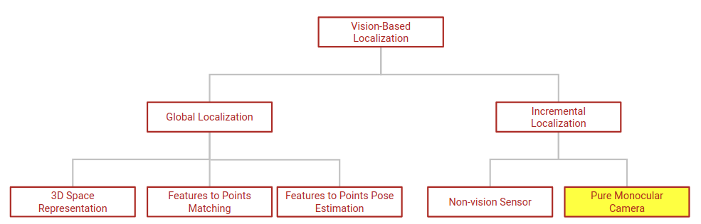
Figure 2.1: Visualization of vision-based localization related work structure

As for the following passages, as shown in 2.1, vision-based localization will be reviewed from two aspects: global localization and incremental localization. As for global localization, I focus on each module of the 3D structure-based VBL pipeline. And as for incremental localization, I concentrate on map-based incremental localization and review from two aspects: systems with non-vision sensors and systems with a pure monocular camera. System with a pure monocular camera, as shown in yellow in 2.1, is where my research locates.

2.2.1 Global Localization

VBL is a broad research topic and has been very active among the computer vision community. Many surveys and reviews have been presented to help researchers to review the existing literature and to narrow down their research interest. Piasco et al. (2018) divide VBL into two distinct families: indirect and direct system. Indirect system also known as image retrieval (Radenović et al. (2016); Arandjelović and Zisserman (2012)) only estimates the coarse camera pose based on a image database. Direct system directly estimate the pose of the query image. Later, Xin et al. (2019) categorized and reviewed VBL based on three different space representations: image database (Arandjelović and Zisserman (2012); Jégou et al. (2010); Torii et al. (2015); Jin Kim et al. (2015); Jégou and Zisserman (2014); Cummins and Newman (2008)), learning model (Shotton et al. (2013); Guzman-Rivera et al. (2014); Valentin et al. (2015); Meng et al. (2016); Brachmann et al. (2016)), and 3D structure (Li et al. (2012); Zeisl et al. (2015); Liu et al. (2017); Sattler et al. (2017); Irschara et al. (2009); Sattler et al. (2011)). According to Xin et al. (2019), method based on 3D structure is the most advance VBL method due to their best performance regarding localization accuracy. Hence, we will focus on direct VBL methods that are based on 3D structure.

3D Space Representation

Structure-based localization methods assume that a scene is represented by a 3D model. The first step of 3D structure-based VBL is to construct the 3D point cloud model using structure from motion (SfM) algorithm. Open source code such as COLMAP developed by Schönberger (2018) and VisualSfM developed by Wu (2013) are commonly used to generate SfM reconstruction from database images. Next, each 3D point needs to associate with a descriptor. Sattler et al. (2011) evaluated different representation for the 3D points and discovered the best representation could be obtained by using all descriptors or the integer mean of all descriptor per visual word.

As for the selection of descriptor, several criteria has to be taken into account: scale, orientation and illumination invariance, as well as computational cost and descriptor vector dimension. Piasco et al. (2018) provided a comprehensive list of descriptors used in VBL. Based on the list, Hessian-affine detector (Mikolajczyk and Schmid (2004)) with SIFT descriptor (Lowe (2004)) is widely used in image retrieve applications. Middelberg et al. (2014) apply RootSIFT (Arandjelović and Zisserman (2012)) to their global localization system to achieve more accurate matching result. Griffith and Pradalier (2017) compared outdoor visual data association with BRIEF (Calonder et al. (2010)), ORB (Rublee et al. (2011b)), SIFT, SURF (Bay et al. (2008)). They discovered all these descriptors performed similarly with a slight qualitative advantage for ORB. Feng et al. (2015) maintained precision and improved rapidity by using BRISK descriptor (Leutenegger et al. (2011a)).

However, traditional features are not robust to weather and illumination changes. Krajník present a trainable feature GRIEF (Generated BRIEF) to solve image registration under variable lighting and naturally-occurring seasonal changes. DeTone et al. (2018b) trained SuperPoint from synthetic data and outperform traditional features in feature matching under illumination changes. Dusmanu et al. (2019) presented D2-Net and shown significantly better performance under challenging conditions, e.g., when matching daytime and night-time images. Sarlin et al. (2019) based on SuperPoint developed a hierarchical localization system that achieved remarkable localization robustness across large variations of appearance.

Features to Points Matching

The next step is to find the correspondences between 2D features and 3D landmark points. The biggest challenge is the efficiency and accuracy. Irschara et al. (2009) proposed to directly obtain the corresponding content in the 3D model through the feature index of the vocabulary tree, instead of linking the images database. Based on the Irschara’s research, Sattler et al. (2011) proposed a vocabulary-based priority search (VPS) method inspired by bag of words matching method. In subsequent work, the same authors Sattler et al. (2016) increased the VPS framework with points to features matching. Sattler et al. (2015) also introduced a visibility chart to improve positioning accuracy. In order to improve the speed of 2d-3d matching, Heisterklaus et al. (2014) introduced MPEG compression method. Donoser and Schmalstieg (2014) trained the random ferns at the top of each point using descriptor redundancy associated with 3D points, and make the speed of 2d-3d matching faster. Feng et al. (2015) used a fast point extractor and adopted a binary descriptor in the method, which greatly increases the calculation speed without affecting the accuracy of the pose estimation.

Features to Points Pose Estimation

The final step is to estimate the camera pose based on features to points correspondences. Defined by Hartley and Zisserman (2003), perspective-n-point (PnP) formulation is the most common tool to recover the absolute camera pose according to the point cloud reconstructed by SfM. Donoser and Schmalstieg (2014), Heisterklaus et al. (2014), and Li et al. (2010) demonstrated that six correspondences between the image and the 3D model are sufficient to retrieve the pose, if we have no information about the intrinsic parameters of the camera. This formulation is known as P6P and can be solved with Direct Linear Transformation (DLT proposed by Hartley and Zisserman (2003)). In particular cases, three correspondences between the image and the model are sufficient (P3P pose computation problem). Irschara et al. (2009) and Middelberg et al. (2014) proof the pose estimation problem can be reduced to a P3P formulation if the intrinsic parameters of the camera are known, or if 3 or more DoF are fixed (Qu et al. (2016); Zeisl et al. (2015)). In those particular cases, P3P solver introduced by Kneip et al. (2011) is mostly used to recover the pose. Works from Förstner and Wrobel (2016) and Zeisl et al. (2015) apply bundle adjustment to refine the initial pose estimation.

Rather than explicitly estimating a camera pose from 2D- 3D matches, some researchers have proposed learning based methods. Brubaker et al. (2013), Brubaker et al. (2015), and Fernández-Moral et al. (2013) proposed CNN-based approaches directly learn to regress a 6 DoF pose from images. However, as shown by Fernández-Moral et al. (2013), such methods do not achieve the same localization accuracy as 3D structure-based algorithms.

2.2.2 Incremental localization

Incremental Visual Localization with Non-Vision Sensor

A lot of literature has presented VO systems to estimate camera poses by detecting and tracking 2D features. However, these incremental-based methods only work well for a short time and drift eventually due to accumulate error. To reduce global error, Zhu et al. (2008) utilized IMU and integrate landmark matching to a pre-built landmark database to improve the overall performance of a dual stereo visual odometry system. They used an intelligent subsample method to reduce the size of the database without dropping the accuracy. Middelberg et al. (2014) developed a scalable and drift-free image-based localization system which tracked camera locally on a mobile device and align the local map with global one in an external server. In their system, imu is used to exploit gravity information. Based on their research, Lynen et al. (2015) presented a large-scale, real-time pose estimation and tracking system that runs on mobile platforms without requiring an external server. Their system employed map and descriptor compression schemes and efficient search algorithm to achieve real-time performance. Surber et al. (2017) developed a robust localization system by decoupling the local visual-inertial odometry from the global registration to the reference map and utilizing GPS as a weak prior for suggesting loop closures.

Incremental Visual Localization with Pure Monocular Camera

In contrast to large scale outdoor localization systems that combine camera and non-vision sensors, localization systems with only a monocular camera are commonly used to navigate robots in constraint areas such as the indoor environment. Alcantarilla et al. (2010) presented a real-time approach for vision-based localization systems within scenes that have been reconstructed offline using SfM. They explored the visibility of individual landmarks to achieve a much faster algorithm and superior localization results. Lim et al. (2012) developed a real-time system to continuously compute precise 6-DoF camera pose, by efficiently tracking natural features and matching them to 3D points in the SfM point cloud.

Recent methods for indoor visual localization typically aim to achieve robustness to changing lighting conditions by relying on map representations that target illumination invariance. This includes approaches using local feature descriptors, which are invariant to affine changes in illumination. Kim et al. (2017) presents an illumination-robust visual localization algorithm for a free-flying robot designed to navigate on the International Space Station (ISS) autonomously. The online image localization algorithm extracts BRISK (Leutenegger et al. (2011b)) descriptors from the query image and match with a prebuilt feature map. Their approach resolved constant lighting changes localization problems but suffered from irregular lighting changes. Caselitz et al. (2020) presented a direct dense camera tracking approach and demonstrated its performance in real-world experiments in scenes with varying lighting conditions.

Chapter 3 Technical Approach

In this chapter, the technical approach will be presented to the reader in two sections: mapping and pose estimation. The mapping and pose estimation sections are presented to help the readers understand the underlying theory of my vision-based localization pipeline.

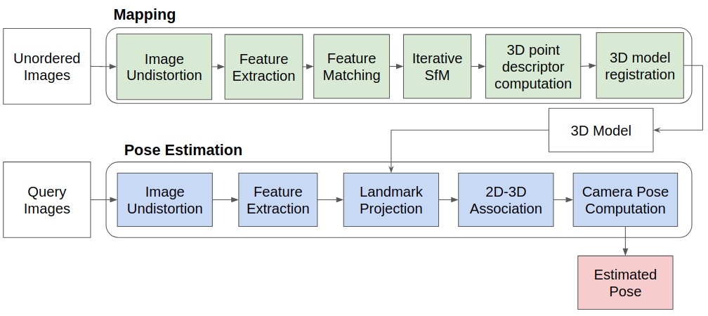
Figure 3.1: This figure is an overview of my localization pipeline.

As shown in 3.1, the task is to build a localization pipeline using a 3D structure-based localization method. The pipeline can continuously estimate the camera pose for every image in a given sequence with a 3D model. This pipeline is developed in a modular structure in that each module can be replaced or improved without influencing the remaining modules.

Before localization, given a set of images, features are extracted from all undistorted images. All features are then matched between every pair of images. The matched features are used to compute the Structure from Motion (SfM) reconstruction. Since SfM does not generate descriptors for the reconstructed 3D points, a descriptor for each 3D point is calculated by creating an elementwise mean descriptor from all feature descriptors mapped to each 3D point. During localization, 3D landmark points are projected into the estimated pose to efficiently filter 3D points that are not within the field of view. The remaining 3D landmark points are matched with 2D features by computing the descriptor distances. The 2D-3D associations are then used to generate a nonlinear least square problem to estimate the camera pose.

3.1 Mapping

The goal of mapping is to create a 3D model that best describes a stationary scene. The mapping pipeline contains six main steps:

1. Image Undistortion.

2. Feature Extraction

3. Feature Matching.

4. Iterative SfM

5. 3D Point Descriptor Computation

6. 3D Model Registration.

3.1.1 Image Undistortion

Image undistortion is to correct the non-linear projection of the surface points of objects onto the image plane due to lens distortion. There are two common types of distortion, tangential distortion and radial distortion. These two types of distortion can be correct with a five parameters undistortion model.

a. Assuming a point $P=\begin{bmatrix}X&Y&Z\end{bmatrix}^{T}$ in the camera frame, its coordinate in the normalized camera frame is:

$$\begin{bmatrix}x\\ y\end{bmatrix}=\begin{bmatrix}X/Z\\ Y/Z\end{bmatrix}$$ (3.1)

b. Correct tangential distortion and radial distortion in the normalized camera frame:

$$\begin{split}x_{distort}=x(1+k_{1}r^{2}+k_{2}r^{4}+k_{3}r^{6})+2p_{1}xy+p_{2}(r^{2}+2x^{2})\\ y_{distort}=y(1+k_{1}r^{2}+k_{2}r^{4}+k_{3}r^{6})+p_{1}(r^{2}+2y^{2})+2p_{2}xy\end{split}$$ (3.2)

c. Finally, project the new point into the pixel coordinate will get the correct position of the point in the image.

3.1.2 Feature Extraction

The process of extracting key points and computing descriptors is called feature extraction. Key points are representative points that can describe an image in a compression way. And key points can still be found in an image when the camera field of view sightly changes. Descriptors are information encoded into features to discriminate features from each other. Different features compute key points and descriptors in different ways. The most common feature descriptor is SIFT. Sift key point is obtained by sliding a Difference of Gaussian filter over the image and detecting local extrema for the filter. The descriptor of Sift is a 128 length vector describing the gradients around the key point.

3.1.3 Feature Matching

Feature Matching is to compare feature descriptors across the images to identify similar features. Comparing descriptors is done by computing the Euclidean distance between them. Because descriptors are usually high dimensional vectors, comparing descriptors from two sets of features is expensive. To decrease the matching time, approximate search is used instead of exhaustively looking for the best match. Approximate search is to use a k-dimensional tree (k-d tree) to store all data. In this way, given a descriptor, the best match or the most similar data can be found by following the path from the top of the tree.

As quoted from Garsten and Smith (2020):

To further ensure that good matches are found it is common to use Lowe’s ratio test to discard matches that are probably to be false. The ratio test takes the ratio of the distance between the first and second nearest neighbors of the descriptor to be matched and evaluates if the ratio is less than a pre-defined threshold. The first nearest neighbor is the most similar descriptor to the matched descriptor, while the second nearest neighbor is the second most similar descriptor. This is expressed as

$$\frac{|d_{i}-d_{N1}|^{2}}{|d_{i}-d_{N2}|^{2}}\leq tol$$ (3.3)

where $d_{i}$ is the descriptor to be matched, $d_{N1}$ and $d_{N2}$ are the first and second nearest neighbor matches and $tol$ is the predefined tolerance. A match passes the ratio test if the ratio is below the threshold. Employing the ratio test ensures that matched descriptors are more similar to each other than to other descriptors. This filters out matches that are unlikely to be correct.

However, in most of the case, a ratio test cannot eliminate false positives. Next, using the RANSCAC algorithm to find the geometry constraint, such as homography matrix, fundamental matrix or essential matrix if the camera calibration matrix is known, can filter bad matches further.

RANSAC

Random Sample Consensus (RANSAC) is a method for picking random data samples to ensures an outlier free subset of data to a certain degree. In many optimization tasks, the data is not perfect. It contains noisy measurements and outliers. Optimizing for all data can then be challenging. Outliers can be far from a correct measurement, contributing to the cost function’s large errors, drowning the effect of errors from accurate measurements. The RANSAC method is widely used to try and find a subset of data that only contains inliers.

$$N=\frac{log(1-p)}{log(1-(1-e)^{s})}$$ (3.4)

RANSAC is solving a problem of using large input data and a solver to compute a solution. The merit of RANSAC is that it can pick a subset of data within the large dataset, which is nearly outlier free, resulting the correct solution’s computation. RANSAC randomly picks a subset of $s$ data points $N$ number of times. $N$ is calculated by 3.4, where $e$ is the ratio between outliers and all matched points, and $p$ represents the desired probability of finding the best solution or model. The outlier ratio $e$ is hard to determine and scarcely available. It can, therefore, be necessary to update the distribution based on inlier results calculated during runtime.

For each iteration, it calculates a solution based on the $s$ data points. Then it calculates an error value for each point within the $s$ points by fitting the point into the solution. For points with an error smaller than a pre-determined threshold are considered as inliers. This procedure is done for all points and will give the number of inliers for a given solution. The number of inliers is used to calculate a new outlier ratio and is then inserted back in 3.4 to calculate the number of iterations needed. Now, each subset $s$ will be associated with a number of inliers and a solution. After all the iterations, the subset $s$ with the maximum inliers is considered as the best subset and the solution associated with the subset is considered the final solution.

3.1.4 Iterative SfM

There are two ways to reconstruct the 3D points and compute the camera poses, incrementally or globally. Global SfM estimates all camera positions and 3D points at the same time. In contrast, incremental SfM adds on one image at a time to grow the reconstruction. Incremental SfM first generate an initial model with a pair of images. New correspondences are found by matching descriptors of new images with the initial model image database. Then 3D points triangulated by new correspondences are added to this initial model. As more images are added, small errors will accumulate, distorting the model. It is common to perform optimization on both 3D point and camera poses with set intervals.

As quoted from Garsten and Smith (2020):

Optimization or more specifically, bundle adjustment is performed to minimize growing errors by shifting the position of 3D points and, depending on how much information about the camera is known, tuning the projection matrix. Localization error is usually quantified as the reprojection error of 3D points. It is computed by taking the square of all 2D image points subtracted by their respectively reprojected 3D point correspondence as

$$e=\sum_{i=1}^{n}\sum_{j=1}^{m}\mathinner{\!\left\lVert(x_{ij}-\frac{p^{1}_{i}\mathbf{X}_{j}}{p^{3}_{i}\mathbf{X}_{j}}),(y_{ij}-\frac{p^{2}_{i}\mathbf{X}_{j}}{p^{3}_{i}\mathbf{X}_{j}})\right\rVert}^{2}$$ (3.5)

3.1.5 3D Point Descriptor Computation

The resulting data from the reconstructions provide 3D points in the SfM coordinate. These 3D points are only described in space $(X,Y,Z)$ and do not have a descriptor assigned to them. Hence the 3D descriptor $\bar{d}$ is computed by taking the mean of the feature point descriptors $d_{i}$ that have been matched to the 3D point. The resulting $\bar{d}=\frac{1}{n}\sum_{i=0}^{n}d_{i}$ is assigned to the 3D point. The mean is used because it is one of the best representations for 3D points, according to Sattler et al. (2011). This results in a 256-long vector describing the 3D-point.

3.1.6 3D Model Registration

The 3D model registration is to constraint the seven degrees of freedom of the 3D model. These seven degrees of freedom includes three degrees of freedom in transition, three degrees of freedom in orientation, and one degree of freedom in scale. A similarity transform will be applied to rescale the model and transform it into a new position and orientation.

$$T_{s}=\begin{bmatrix}sR&t\\ 0&1\end{bmatrix}$$ (3.6)

where $s$ is the scaling factor, $R$ is a 3x3 rotation matrix and $t$ is a 3x1 translation vector.

3.2 Pose estimation

The methodology behind this is to find the current frame observed landmark points in the sparse map and estimate the pose by employing a nonlinear solver on the current pose. The localization system can be described within the Bayesian filtering framework.

$$\underbrace{P(X_{t}|Z^{1\mathrel{\mathop{\mathchar 58\relax}}t},L)}_{Posterior}\propto\underbrace{P(z_{t}|X_{t},L)}_{Measurement}\cdot\int_{\theta_{t-1}}\underbrace{P(X_{t}|X_{t-1})}_{Motion}\underbrace{P(X_{t-1}|Z^{t-1},L)}_{Prior}dX_{t-1}$$

Where L is a set of high quality landmarks reconstructed from the images and $Z^{1\mathrel{\mathop{\mathchar 58\relax}}t}\equiv z_{t}$ indicates the sequence of images up to time t.

There are 5 modules in pose estimation:

1. Image Undistortion

2. Feature Extraction

3. Landmark Projection

4. 2D-3D Association

5. Camera Pose Computation

The first two are the same as in the mapping section, so we only cover the last three below:

3.2.1 Landmark Projection

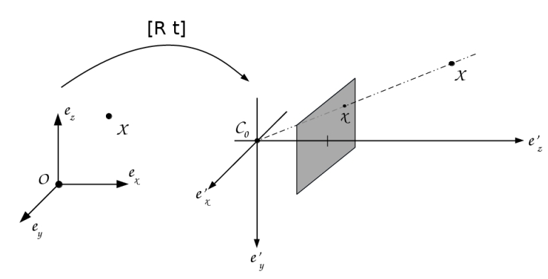
Figure 3.2: Visualization of applying the camera extrinsics will transform a 3D point from global coordinates into the camera coordinate system. Image adopt from Garsten and Smith (2020)

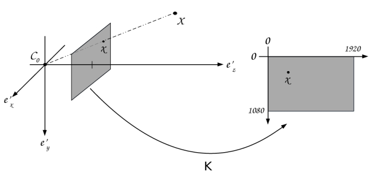
Figure 3.3: Applying the calibration matrix K to a point in camera coordinates will reproject it into the image as a pixel coordinate. Image adopt from Garsten and Smith (2020)

The camera model describes the process of projecting a point in the 3D world to a 2D image plane. There are many types of camera models. Different camera models are used to describe different kinds of camera lenses. The simplest camera model is the pinhole camera model. The pinhole camera model is a very common and efficient model that describes image rays pass through a pinhole from the front of the pinhole and generates an image by intersecting the image plane at the back of the pinhole. The pinhole is the camera center where all image rays intersect.

An image pixel coordinate $\begin{bmatrix}u&v\end{bmatrix}^{T}$ can be calculated by projecting the global point $\begin{bmatrix}X&Y&Z\end{bmatrix}^{T}$ into the image with a projection matrix $P$:

$$\lambda\underbrace{\begin{bmatrix}u\\ v\\ 1\end{bmatrix}}_{\bar{x}}=P\underbrace{\begin{bmatrix}X\\ Y\\ Z\\ 1\end{bmatrix}}_{\bar{X}}$$ (3.7)

where $\lambda$ is a scaling parameter. $\begin{bmatrix}u&v&1\end{bmatrix}^{T}$ and $\begin{bmatrix}X&Y&Z&1\end{bmatrix}^{T}$ are represented in homogeneous coordinates. Homogeneous coordinates lift an N-dimensional point to an N+1 dimensional line. The N-dimensional point can be retrieved after a transformation by dividing by the last entry and then dropping the last entry:

$$P=K\begin{bmatrix}R&t\end{bmatrix}$$ (3.8)

where R is a 3x3 rotation matrix, t is a 3x1 translation vector, and K is a 3x3 calibration matrix. This compact way of applying $R$, $t$ and $K$ requires the use of homogeneous coordinates. $R$ and $t$ are called the camera extrinsics, which provides the camera orientation and position information. $K$ is the camera intrinsics, which describes the property of the camera. Unlike the camera extrinsics, the camera intrinsics do not change when the camera is moving. As seen in 3.2, the rotation $R$ and translation $t$ transform a point from a world coordinate system into a camera coordinate system. As seen in 3.3, from a camera coordinate system, points can then be re-projected into the pixel coordinate system by applying the camera calibration matrix $K$ because the calibration matrix transformed distances into pixel values. The calibration matrix for a pinhole camera looks like

$$K=\begin{bmatrix}f_{x}&s&c_{x}\\ 0&f_{y}&c_{y}\\ 0&0&1\end{bmatrix}$$ (3.9)

where the parameters are; $f_{x}$ and $f_{y}$ are the focal lengths along the x and y coordinate axes of the pixel coordinate system. Skew $s$, which describes the tilt of the pixels in the image. Finally, $c_{x}$ and $c_{y}$ maps the origin from where the z-axis intersects the image plane to the upper left pixel.

3.2.2 2D-3D Association

The 2D-3D association is to match 2D features with 3D landmarks. 2D features can be matched with 3D landmarks by comparing the L2 distance of their descriptors or comparing the pixel distance of 3D landmark projected features with the extracted features. Same as the feature matching process, before the comparison of descriptors, data are arranged into a k-d tree. The best match is the descriptor pair with the smallest L2 distance. However, this method is highly inaccurate, especially when a lot of 3D landmark points are similar in descriptors. To efficiently filter the outliers, the geometry relationship between 3D landmarks and 2D features can be taken into account. Since the projected point of the matched 3D landmark point should be close to the extracted feature point. Projected points that are far away from their corresponding extracted feature points can be rejected.

3.2.3 Camera Pose Computation

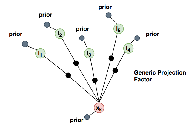
Figure 3.4: Pose Estimation Factor Graph. The Factor Graph contains five prior factors, five landmarks $\ell_{i}$, and one camera pose $x_{k}$. The estimation of $x_{k}$ is the pose of the previous state. The generic projection factors represented by the black nodes are the 2D to 3D correspondences.

Camera pose can be computed by solving a nonlinear least square problem formulated by the 2D-3D association. As shown in 3.4, the nonlinear least square problem can be presented as a factor graph. Each 2D-3D correspondence formulates a generic projection factor. Each point variable is attached to a prior factor.

The error function of a projection factor:

$$e_{projection}=||K(RX+t)-p||_{2}$$

where $K$ is the camera calibration matrix, $R$ and $t$ is the camera rotation matrix and translation matrix. $p$ is the extracted feature point.

The error function of a prior factor:

$$e_{prior}=||\hat{P}-P||_{\sum}$$

where P̂ and P can be both 3 dimension point or 6 dimension pose.

The optimization Equation:

$$X^{MAP}=\underset{X}{argmin}\sum_{i}(e_{i})^{2}$$

Factor Graph

As quoted from Dellaert (2012b):

Factor graphs are graphical models (Koller and Friedman (2009)) that are well suited to modeling complex estimation problems, such as Simultaneous Localization and Mapping or SfM. You might be familiar with another often used graphical model, Bayes networks, which are directed acyclic graphs. A factor graph, however, is a bipartite graph consisting of factors connected to variables. The variables represent the unknown random variables in the estimation problem, whereas the factors represent probabilistic information on those variables, derived from measurements or prior knowledge.

Chapter 4 Implementation Details

4.1 Blimp Configuration

The blimp platform is based on an infrared remote control commercial toy blimp, which used a motor control fishtail to provide a forward thrust and a trackpad to adjust its altitude. A AAA battery powers the motor control fishtail and trackpad. Moreover, three additional fins attached on the blimp surface are used to stabilize the blimp while flying.

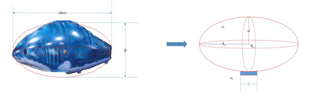
Figure 4.1: Autonomous Blimp Envelope Figure, adopt from Wan et al. (2018)

As it’s shown in Figure 3.1, a flying toy ‘shark’, which is an inflatable balloon, was selected as the envelope. According to Wan et al. (2018), the shape of the blimp is approximated by an ellipsoid with $[R_{a};R_{b};R_{c}]$ defined as the three semi-major axes. The volume of the envelope is estimated as Vb =$190.5cm^{3}$. According to Archimedes Principle, the maximum payload capacity is calculated by:

$$m_{load}=V_{b}\cdot(\rho_{air}-\rho_{helium})=202.1g$$

where $\rho_{helium}=169.3g/cm^{3}$ and $\rho_{air}=1226.0g/cm^{3}$.

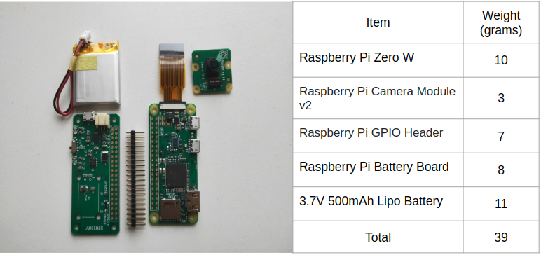
Figure 4.2: Perception Hardware System

I designed a lightweight perception hardware system that includes a raspberry pi zero, a raspberry pi camera, and a Lipo battery, which can be attached to the surface of the envelope.

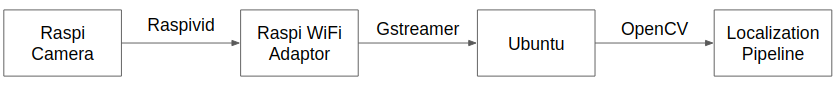
Figure 4.3: Video Transmission Pipeline

Video sequences captured by the raspberry pi camera are first processed by Raspivid, which is a package provided by the raspberry pi to access the video captured with the camera module. The video is then transferred to an Ubuntu system in the ground station through WiFi. This process is done with Gstreamer, which is an open-source tool to handle video streaming. After setting up the Gstreamer server and client to establish the connection, OpenCV can be used to capture video streams from the Linux client.

4.2 Mapping

To reconstruct the 3D model, I first held the perception hardware system (4.2) by hand and collected unordered images from the Atrium. With the unordered images, I undistorted the images based on the camera calibration matrix through OpenCV. Next, I extracted SuperPoint features and 256-dimensional descriptors that describe the respective points from the undistorted images with the SuperPoint pretrained network. The data is then processed in feature matching by matching the descriptors between every image pairs through OpenCV. I used ratio test and RANSAC introduced by Fischler and Bolles (1981) to filter bad matches. As for RANSAC, I used a python library called pydegensac which includes LO-RANSAC designed by Chum et al. (2003) and DEGENSAC designed by Chum et al. (2005). This library is marginally better than OpenCV RANSAC. The feature extraction and feature matching data are then stored in a database file.

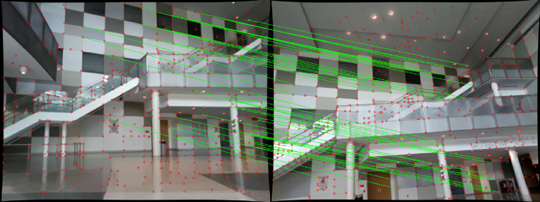
Figure 4.4: Feature matching with SuperPoint and pydegensac.

I then stored all data in a database file and used COLMAP developed by Schönberger (2018) to finish the final reconstruction through an iterative method. This results in a SuperPoint-based 3D reconstruction. In contrast, to reconstruct the 3D model with Sift features, I do not need to create a database file. I only need to input the unordered images into COLMAP and run COLMAP feature extraction, feature matching, and reconstruction. This is because COLMAP is implemented with Sift feature extraction and matching. The resulting reconstruction, as shown in 4.5, is defined up to an arbitrary scaling factor compared to the real-world 3D model.

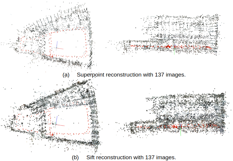
Figure 4.5: COLMAP 3D Reconstruction Result with SuperPoint and Sift Descriptors

The result from COLMAP does not contain the descriptors for the 3D points. Hence, I use the database file and the COLMAP reconstruction output files to create a new data structure named map containing the 3D points and the 3D point descriptors.

The reconstruction results were then registered to the real world scale by comparing it with the building floorplans. I first selected pairs of points in the reconstructed 3D models and found their correspondences in the building floorplans. Next, I recovered the scale by calculating the point distance differences. The scale is up to a scale factor of 1.2.

4.3 Pose Estimation

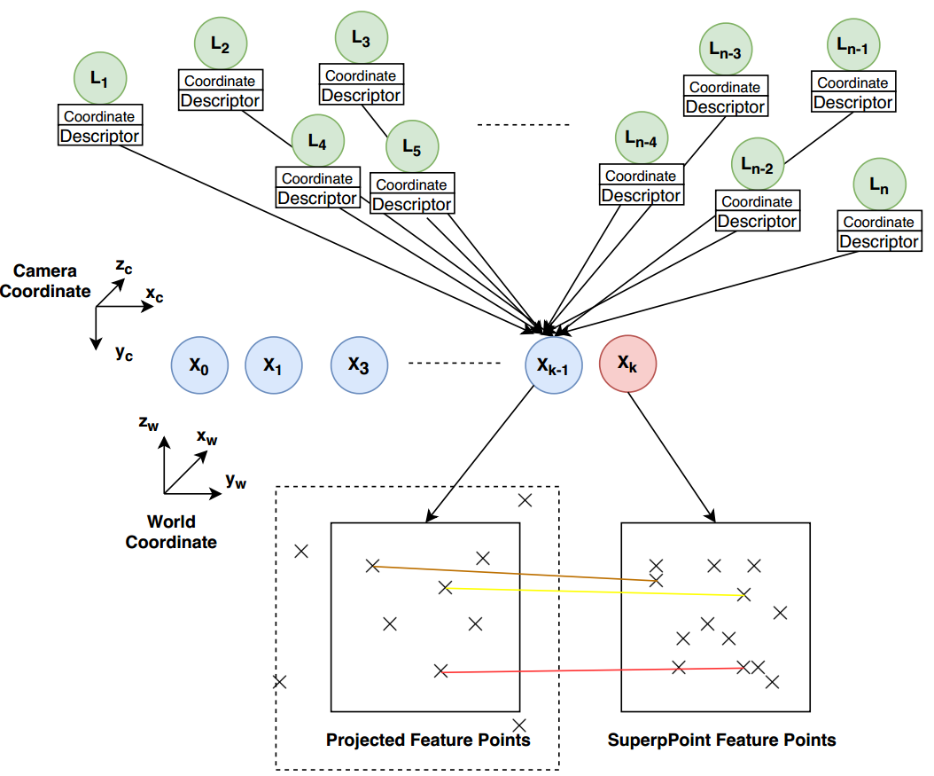
Figure 4.6: Camera Tracking. Feature points projected outside the image are invalid projected points.

The camera tracking or incremental pose estimation process is presented in 4.6. 3D points from the sparse point cloud are projected to the estimated camera pose (3.7) with points behind the camera or out of the range of the image filtered. In my pipeline, I assumed the camera motion is static due to the slow-motion of a blimp. Hence the 3D points are projected to the pose of the previous state.

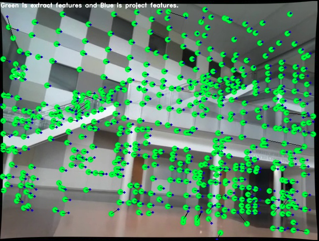
Figure 4.7: The blue dots are the projected features, and green circles are the extracted features. The extracted features are displayed in a large green circle for better visualization purposes.

Next, SuperPoint features are extracted from the current undistorted input frame. Measurements, which are the correspondences of 3D landmark points and 2D features, are then obtained by matching between the projected 2D features and the extracted 2D features. The matching criteria are the pixel distance and the L2 distance between descriptors.

Finally, the current pose is obtained with a nonlinear solver represented by a factor graph, as shown in 3.4.

Result: An estimate trajectory

Read 3D model and initial pose;

$trajectory=[initial\_pose]$;

while True do

       Read a new frame;

       Calculate estimate pose based on the camera motion model;

       if $frame\>entropy>minimal\>entropy$ then

             Undistort image and extract SuperPoint features;

             Project 3D landmarks into the estimate pose;

             Filter projected points that are behind the camera or out of the range of the image;

             for SuperPoint feature in SuperPoint features do

                   Use KNN to find all project landmarks around the SuperPoint feature within a radius threshold;

                   Find the project landmark with the smallest descriptor distance;

                   if $smallest\>descriptor\>distance<maximum\>distance$ then

                         Append 2D feature point and 3D landmark point into an observation list;

                        

                  else

                         continue

                   end if

                  

             end for

            if $number\>of\>observations>minimal\>observation$ then

                   Use the observation list to construct a Factor Graph with generic projection factor and Huber noise model;

                   Optimize Factor Graph with Gauss Newton optimizer;

                  

            else

                   continue;

                  

             end if

            

      else

             continue;

       end if

      

end while

Algorithm 1 Visual Based Localization

Chapter 5 Experiments and Results

In this chapter, evaluation experiments will be performed with the localization system to show the readers how the localization result is affected by different factors, such as illumination, descriptor, 3D model density and, etc. I will first introduce the experiment setup, trajectory error metrics, and ground truth to help readers understand the experiments’ process and evaluation metrics.

5.1 Experimental Setup

For all programs and tests, I ran on a standard laptop PC on a 64-bit Ubuntu 18.04 system. The laptop is equipped with an Intel Core i7-9750H 2.60Hzx12 CPU, 16GB DDR, and an Nvidia Geforce RTX 2060 GPU card. The sensor I used is a raspberry pi camera v2.1 (rolling shutter) with a 640x480 resolution and a frame rate of up to 30Hz. All experiments are conducted within the Georgia Institute of Technology Klaus Atrium.

5.2 Trajectory Error Metrics

Zhang and Scaramuzza (2018) proposed the evaluation method used for the following experiments. As shown in 5.1, the estimation $\hat{\mathbf{X}}$ is transformed to the aligned estimation $\hat{\mathbf{X^{\prime}}}$ before the evaluation. Because I am using a monocular camera, this transformation from the estimate trajectory to the aligned estimate trajectory is a similarity transform. Next I calculated the absolute trajectory error (ATE) with the groundtruth $\mathbf{X}_{gt}$ and the aligned estimation $\hat{\mathbf{X^{\prime}}}$.

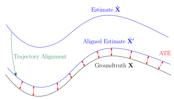
Figure 5.1: ATE, adopt from Zhang and Scaramuzza (2018)

The evaluation of a single state:

($\angle(\cdot)$ means converting to angle, $log(\cdot)$ returns the canonical coordinates in Lie group)

$$orientation\ error=\Delta{R_{i}}=\angle(\mathinner{})$$

$$position\ error=\Delta{\mathbf{p}_{i}}=\mathinner{}$$

The root mean square error (RMSE) is then used to quantify the quality of the whole trajectory.

$$ATE_{rot}=(\frac{1}{N}\sum_{i=o}^{N-1}\Delta{R_{i}}^{2})^{\frac{1}{2}}$$

$$ATE_{pos}=(\frac{1}{N}\sum_{i=o}^{N-1}\Delta{\mathbf{p}_{i}}^{2})^{\frac{1}{2}}$$

5.3 Ground Truth

I will use the result from SfM as the ’ground truth’ since SfM is currently the most accurate visual reconstruction method. Moreover, the reconstruction area is large to set up a pose tracking system. Thus I used COLMAP to reconstruct all the camera poses with Sift descriptors. The results from COLMAP are used as my ’ground truth’ for evaluations of all of the following experiments.

5.4 Evaluations

5.4.1 Repeating Pattern, and Rolling Shutter

Repeating pattern and rolling shutter effect are two common problems that cause mismatches during 2D-2D feature matching and 2D feature to 3D landmark point association which can further influence pose estimation. Because I experimented with a rolling shutter camera in an environment full of repeating patterns (5.2), therefore I do not specifically design experiments to demonstrate that my pipeline can overcome these two problems. Instead, if I can perform one successful trajectory estimation within my selected environment, a close loop localization result, I can prove that my pipeline overcomes the repeating pattern and rolling shutter problem.

(a)

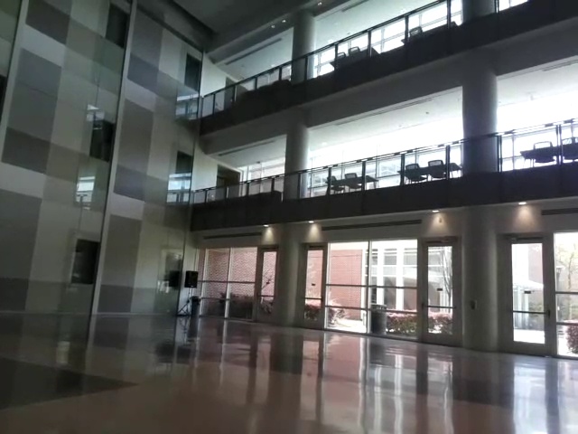
(b)

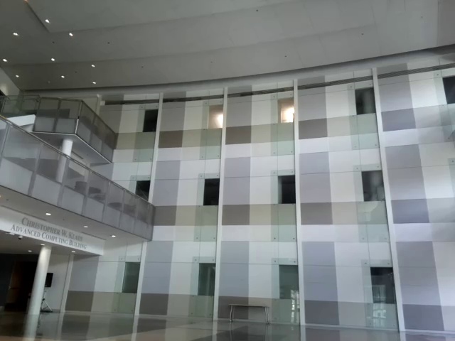
(c)

Figure 5.2: Klaus Atrium

5.4.2 Traditional Descriptor vs Learning Descriptor

I designed my first experiment to compare the effect of the descriptor on my pipeline. To analyze the results between traditional descriptor and learning-based descriptor, I selected Root Sift as the traditional descriptor representative due to its popularity and outstanding performance among visual based localization. Because my pipeline runs with SuperPoint by default, hence the comparison is between Root Sift and SuperPoint.

Experiment Setup

I collected a training dataset and a test dataset. Both datasets are collected in a similar trajectory and under same illumination. The datasets are collected by holding the perception system by hand. The training dataset, which is used to reconstruct the sparse point cloud model, contains 137 images. I used the training dataset to reconstructed two sparse point cloud models, one with Sift feature descriptor and one with SuperPoint feature descriptors (4.5). I used the Sift point cloud to perform localization with Root-Sift and used the SuperPoint point cloud to perform localization with SuperPoint.

Result

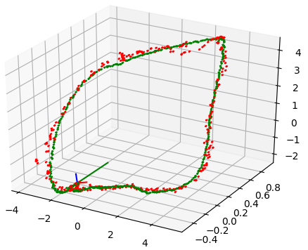
(a)

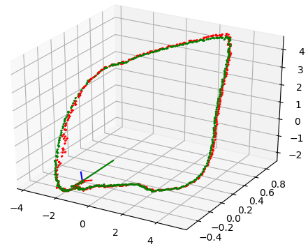
(b)

Figure 5.3: Root Sift and SuperPoint

Red is the aligned estimate trajectory. Green is the ground truth trajectory. The aligned estimate trajectory is downsampled from the actual trajectory and contains 387 images.

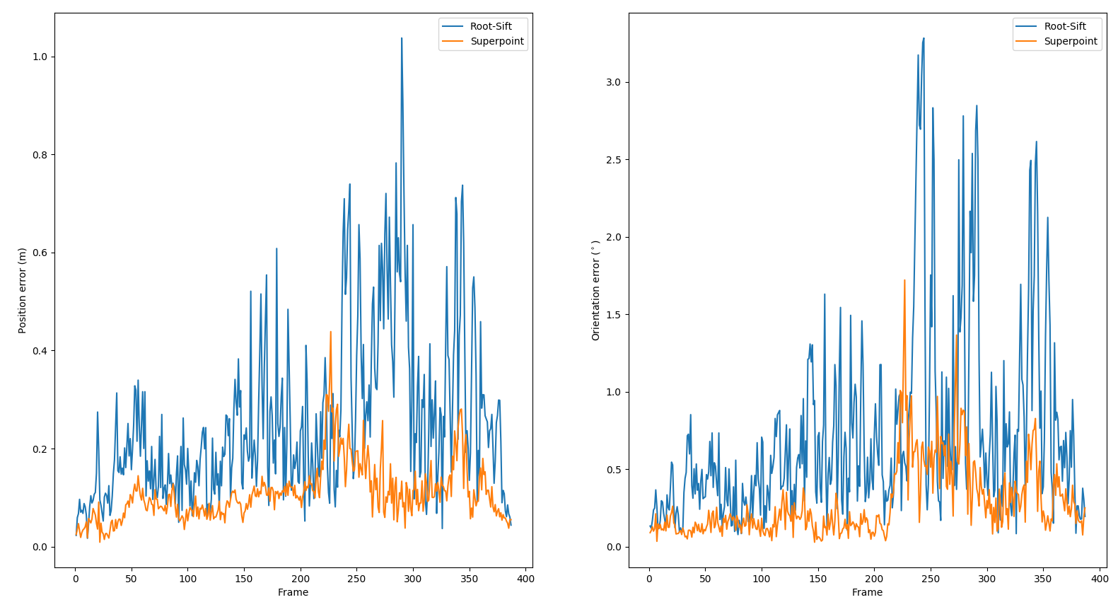
Figure 5.4: SuperPoint and Root Sift trajectory errors

Table 5.1: ATE results of SuperPoint and Root-Sift

	$ATE_{pos}(m)$	$ATE_{rot}(^{\circ})$
SuperPoint	0.123	0.369
Root-Sift	0.305	0.955

Discussion

From the result, we can observe that both the Root Sift trajectory result and SuperPoint trajectory result are closed to the ground truth trajectory result. But SuperPoint demonstrates higher localization accuracy than Root Sift.

5.4.3 Illumination

Experiment Setup

I collected one training dataset and four test datasets. All datasets are collected under similar trajectories but different illumination conditions. I used the training data to build the 3D model and executed the localization pipeline on all test datasets with SuperPoint descriptor.

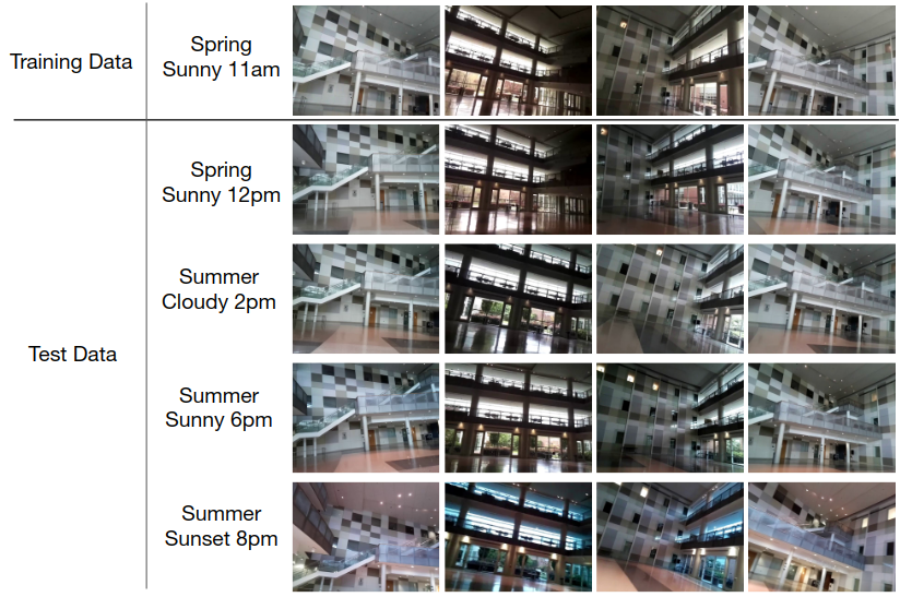
Figure 5.5: Datasets under different illuminations

Result

(a)

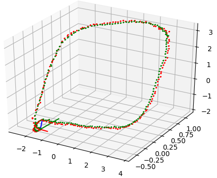
(b)

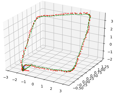
(c)

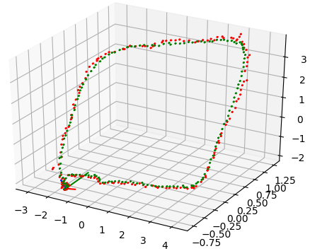
(d)

Figure 5.6: Localization results under different illuminations

Red is the aligned estimate trajectory. Green is the ground truth trajectory. The lengths of different test datasets are different.

Table 5.2: ATE results of different illuminations

Datasets	SuperPoint Descriptor
	$ATE_{pos}(m)$	$ATE_{rot}(^{\circ})$
Spring Sunny 12pm	0.123	0.369
Summer Cloudy 2pm	0.255	0.669
Summer Sunny 6pm	0.31	0.622
Summer Sunset 8pm	0.298	0.714

Discussion

The result from 5.2 and 5.5 indicates that my pipeline can run on datasets that are collected under illumination different from the training data. The Spring Sunny 12 pm dataset is the most accurate because the trajectory and illumination are similar to the training dataset. The other three datasets contain more degenerated frames caused by the motion blur effect. These degenerated frames increased the error of the final result.

5.4.4 Large field of view changes and 3D Model Density

Experiment Setup

To test how viewpoint changes will affect the localization result, I collected the training data in a large circle with all the camera facing inside the Atrium. Then, I collected the test data in a small circle with all the camera facing forward. I later collected additional images that can be added to the training data to reconstruct 3D models of two different densities.

Result

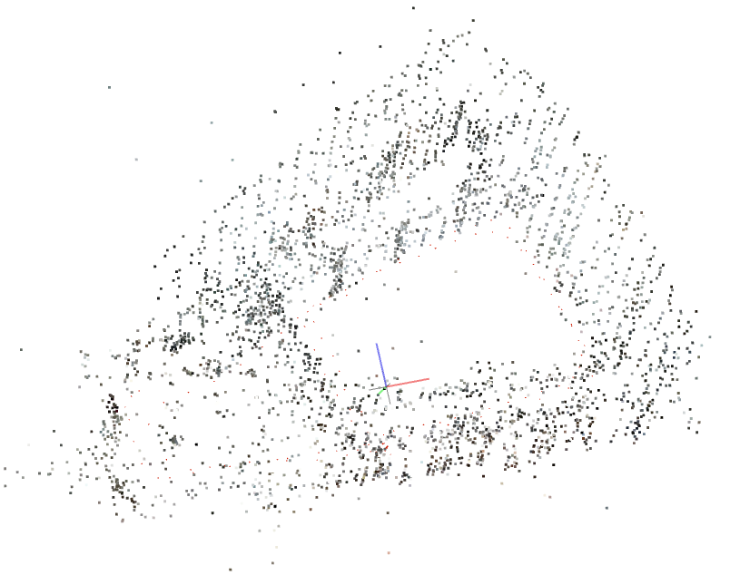
(a)

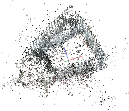
(b)

Figure 5.7: Map with different density

The sparse map is reconstructed with 126 images and contains 4077 points. The dense map is reconstructed with 513 images and contains 10507 points.

(a)

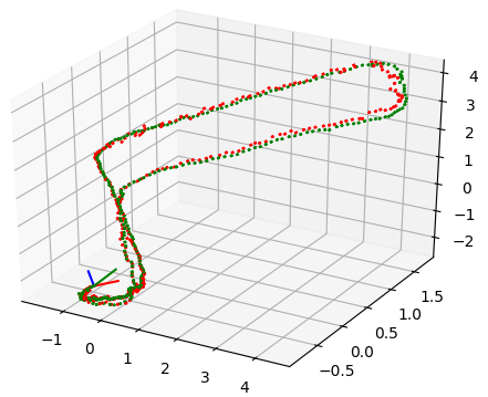
(b)

Figure 5.8: Trajectory with different density maps

Red is the aligned estimate trajectory. Green is the ground truth trajectory.

Table 5.3: ATE results of different illuminations

	Sparse Map	Dense Map
$ATE_{pos}(m)$	0.311	0.268
$ATE_{rot}(^{\circ})$	0.701	0.567
average SuperPoint extraction time $(s)$	0.0831079	0.0711602
average landmark projection time $(s)$	0.000665298	0.00112228
average success projected landmarks	1089.8	2614.35
average 2D-3D data association time $(s)$	0.159091	0.1665
average pose estimation time $(s)$	0.0126785	0.0139296
average total time $(s)$	0.260967	0.256019

Discussion

As seen in 5.8(b), the pipeline can estimate the trajectory even when the test data viewpoint is much different from the training dataset. This is because SuperPoint descriptors are invariant to viewpoint changes. Thus 2d features and 3d landmarks can still be matched together even when their associated descriptors are generated under different viewpoints.

As for how the map density will affect the localization result, from 5.3 we can see that localization under dense map not only results in higher accuracy but also surprisingly results in lower computation time than localization under sparse map. This is because the main factor of the computation time is SuperPoint extraction time and 2D-3D data association time. The density of the map does not affect the feature extraction step. It also has less effect on 2D-3D data association time because in my pipeline within the 2D-3D data association step, I iterative through all SuperPoint features instead of projected landmarks.

5.4.5 Motion Model

Experiment Setup

I hope to compare how different motion models will affect the localization result. Hence, apart from the static motion model, which is the default motion model used in my pipeline, I also applied a constant speed motion model in the experiment. I used the same dataset from the 3D model density experiment to complete this experiment.

Static motion model:

$${}_{w}T_{k+1}={}_{w}T_{k}$$ (5.1)

Constant speed motion model:

$$\begin{split}{}_{k+1}T_{k}={}_{k}T_{k-1}\\ {}_{w}T_{k+1}={}_{w}T_{k}*{}_{k}T_{k-1}\end{split}$$ (5.2)

where ${}_{w}T_{k}$ is the 6 DoF pose in the world coordinate system at $k$ time step. ${}_{k}T_{k-1}$ is the transformation from $k-1$ time step pose to the $k$ time step pose.

Result

Table 5.4: Map Density and Motion Model

	$ATE_{pos}(m)$	$ATE_{rot}(^{\circ})$
Sparse Map Static Speed	0.704	0.311
Sparse Map Constant Speed	0.640	0.311
Dense Map Static Speed	0.567	0.268
Dense Map Constant Speed	0.501	0.265

(a)

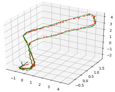
(b)

(c)

(d)

Figure 5.9: Trajectory with different motion model

Red is the aligned estimate trajectory. Green is the ground truth trajectory.

Discussion

As shown in 5.4 and 5.9(d), a better motion model result in a more accurate trajectory because it provides better pose prior and 2D-3D association during the pose estimation. The best combination for my pipeline is a dense map combine with a constant speed motion model.

5.4.6 Fast-Motion Dataset

Experiment Setup

In all previous experiments, all datasets are collected at a slow-motion because the localization system is designed for a slow-motion blimp that moves around at the speed of approximately $1m/s$ for translation and $10^{\circ}/s$ for rotation.

In this experiment, I hope to test how a fast-motion dataset input will affect the localization result. Based on the previous experiments, I know that a density map with a constant speed model is the best combination for my pipeline. Thus, I collected a training dataset with 515 images to reconstruct a dense map. The dense map contains 10,591 points. The test dataset is collected at the speed of around $4,\text{m/s}$ for translation and $45^{\circ}/\text{s}$ for rotation. Because of the fast motion, the dataset contains a lot of frames with strong motion blur and rolling shutter effects.

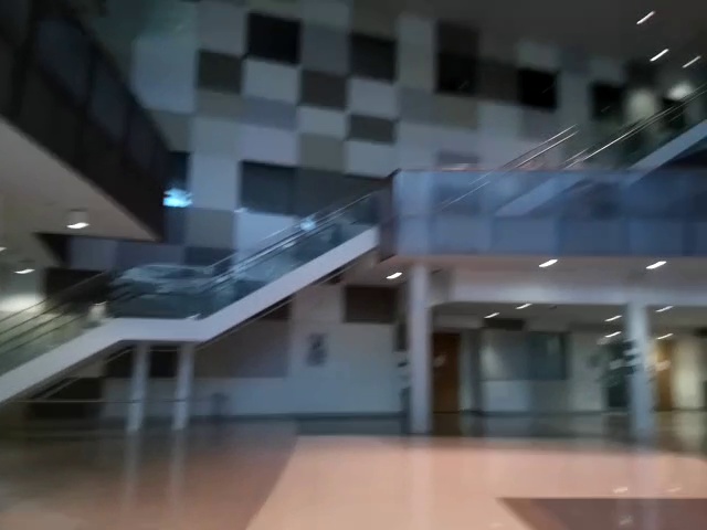
(a)

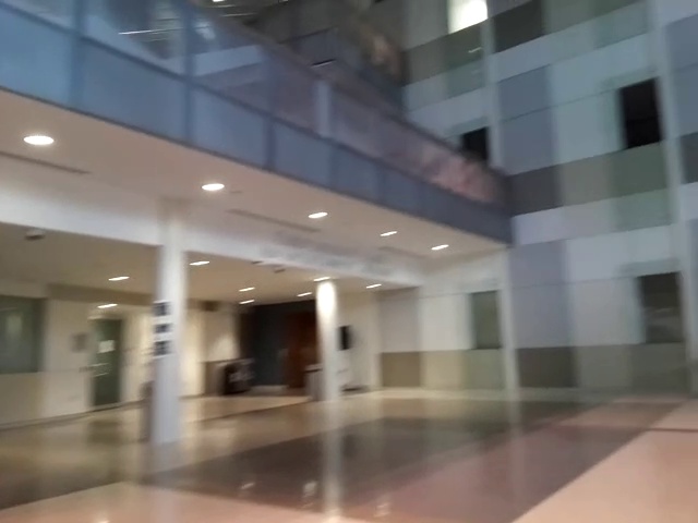
(b)

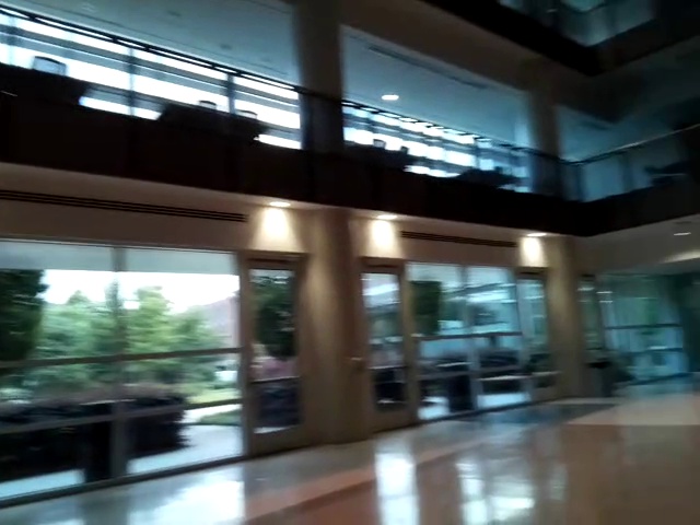
(c)

Figure 5.10: Motion Blur Frames

Result

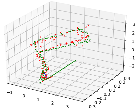
(a)

Figure 5.11: Fast Motion Dataset Result

Table 5.5: ATE results of fast motion dataset

$ATE_{pos}(m)$	$ATE_{rot}(^{\circ})$
1.178	0.379

Discussion

From the result, we can observe that the pipeline can only roughly estimate the trajectory of the camera with a high error. This result shows that my pipeline is not robust to fast-motion camera movement, because the motion-blur effect that normally exists for several frames causes translation and rotation drift during pose estimation.

Chapter 6 Conclusion

Vision localization based on a prebuilt map is becoming increasingly popular recently. In this thesis, an indoor incremental localization pipeline has been implemented based on SuperPoint descriptor. The pipeline utilizes a motion model to associate 3D landmarks with 2D features. In this way, I developed an incremental localization solution based on conventional global vision-based localization structures. The pipeline can continuously estimate camera poses based on a sparse map and an initial pose. Several experiments have been conducted on the pipeline. The results indicate that the pipeline is robust to illumination and viewpoint changes. And the pipeline is not affected by repeating patterns and rolling shutter effects. By comparing localization results on different descriptors, it is clear that SuperPoint based localization is more accurate than and Root Sift based localization. Finally, my raspberry pi based perception system can be easily integrated into blimp or other miniature low-cost robots.

Chapter 7 Future Work

In this thesis, I have presented some results for incremental localization in an indoor environment. The developed pipeline has a lot of potential for improvements as it is only a first implementation where the amount of optimization has been minimal. For example, this pipeline requires an initial pose to begin trajectory estimation. In this case, pose estimation failure will terminate the trajectory estimation process. To order to solve this problem, I can integrate a global localization module into the system.

Moreover, I believe each pose estimation factor graph can be added to a large factor graph constructed by the points and poses from the SfM process. In this way, the occlusion problem can be solved by considering each observation’s observability during the pose estimation.

In addition, the current implementation sets the minimal descriptor distance within the 2D-3D association as a fixed value. I believe this value can be studied during the localization process. By doing so, the 2D-3D association process would contain fewer outliers and result in more accurate pose estimation.

As applications for incremental localization usually requires real-time performance, the next step would be to create a pipeline capable of real-time localization and record benchmarks for comparison to other localization methods. To increase computation speed, I can convert loop-based modules written in python into C++ code or use a more advanced desktop than a laptop. I can further study the focus of features in the image to reduce computation on the 2D-3D association.

Finally, the current experiments are not tested on the blimp because I have not developed the blimp control system. In the future, operations can be conducted by attaching the hardware system on a blimp. If the system runs on the blimp, I hypothesis that one of the main differences is the input sequence will contain more blurry effects caused by the unstable movement of the blimp. Luckily this problem can be eliminated if we know the motion model of the blimp.

References

- Müller (2013) Jörg Müller. Autonomous navigation for miniature indoor airships. Diss. University ”a tsbibliothek Freiburg, 2013.
- Kim et al. (2017) Pyojin Kim, Brian Coltin, Oleg Alexandrov, and H Jin Kim. Robust visual localization in changing lighting conditions. In 2017 IEEE International Conference on Robotics and Automation (ICRA), pages 5447–5452. IEEE, 2017.
- Lim et al. (2012) Hyon Lim, Sudipta N Sinha, Michael F Cohen, and Matthew Uyttendaele. Real-time image-based 6-dof localization in large-scale environments. In 2012 IEEE Conference on Computer Vision and Pattern Recognition, pages 1043–1050. IEEE, 2012.
- Fukao et al. (2003) Takanori Fukao, Kazushi Fujitani, and Takeo Kanade. An autonomous blimp for a surveillance system. In Proceedings 2003 IEEE/RSJ International Conference on Intelligent Robots and Systems (IROS 2003)(Cat. No. 03CH37453), volume 2, pages 1820–1825. IEEE, 2003.
- Yamada et al. (2009) Tatsuya Yamada, Takehisa Yairi, Suay Halit Bener, and Kazuo Machida. A study on slam for indoor blimp with visual markers. In 2009 ICCAS-SICE, pages 647–652. IEEE, 2009.
- Al-Jarrah et al. (2013) Rami Al-Jarrah, Radouane Ait Jellal, and Hubert Roth. Blimp based on embedded computer vision and fuzzy control for following ground vehicles. IFAC Proceedings Volumes, 46(29):7–12, 2013.
- Milford and Wyeth (2012) Michael J Milford and Gordon F Wyeth. Seqslam: Visual route-based navigation for sunny summer days and stormy winter nights. In 2012 IEEE International Conference on Robotics and Automation, pages 1643–1649. IEEE, 2012.
- Ng and Henikoff (2003) Pauline C Ng and Steven Henikoff. Sift: Predicting amino acid changes that affect protein function. Nucleic acids research, 31(13):3812–3814, 2003.
- Bay et al. (2006) Herbert Bay, Tinne Tuytelaars, and Luc Van Gool. Surf: Speeded up robust features. In European conference on computer vision, pages 404–417. Springer, 2006.
- Rublee et al. (2011a) Ethan Rublee, Vincent Rabaud, Kurt Konolige, and Gary Bradski. Orb: An efficient alternative to sift or surf. Proceedings of the IEEE International Conference on Computer Vision (ICCV), 34(5):2564–2571, 2011a.
- DeTone et al. (2018a) Daniel DeTone, Tomasz Malisiewicz, and Andrew Rabinovich. Superpoint: Self-supervised interest point detection and description. In CVPR Deep Learning for Visual SLAM Workshop, 2018a. URL http://arxiv.org/abs/1712.07629.
- Alcantarilla et al. (2010) Pablo F Alcantarilla, Sang Min Oh, Gian Luca Mariottini, Luis M Bergasa, and Frank Dellaert. Learning visibility of landmarks for vision-based localization. In 2010 IEEE International Conference on Robotics and Automation, pages 4881–4888. IEEE, 2010.
- Dellaert et al. (2017) Frank Dellaert, Michael Kaess, et al. Factor graphs for robot perception. Foundations and Trends® in Robotics, 6(1-2):1–139, 2017.
- Dellaert (2012a) Frank Dellaert. Factor graphs and gtsam: A hands-on introduction. Technical report, Georgia Institute of Technology, 2012a.
- de Paiva et al. (2006) Ely Carneiro de Paiva, José Raul Azinheira, Josué G Ramos Jr, Alexandra Moutinho, and Samuel Siqueira Bueno. Project aurora: Infrastructure and flight control experiments for a robotic airship. Journal of Field Robotics, 23(3-4):201–222, 2006.
- Lacroix (2000) Simon Lacroix. Toward autonomous airships: research and developments at laas/cnrs. In 3rd International Airship Convention and Exhibition. Friedrichshafen (Germany), juillet. Citeseer, 2000.
- Lacroix et al. (2002) Simon Lacroix, Il-Kyun Jung, Philippe Soueres, Emmanuel Hygounenc, and Jean-Paul Berry. The autonomous blimp project of laas/cnrs-current status and research challenges. In Proceeding of the International Conference on Intelligent Robots and Systems, IROS, Workshop WS6 Aerial Robotics, pages 35–42. Citeseer, 2002.
- Hygounenc et al. (2004) Emmanuel Hygounenc, Il-Kyun Jung, Philippe Soueres, and Simon Lacroix. The autonomous blimp project of laas-cnrs: Achievements in flight control and terrain mapping. The International Journal of Robotics Research, 23(4-5):473–511, 2004.
- Wimmer et al. (2002) Dirk-A Wimmer, Michael Bildstein, Klaus H Well, Markus Schlenker, Peter Kungl, and BH Kröplin. Research airship” lotte” development and operation of controllers for autonomous flight phases. In Workshop on aerial robotics, IEEE international conference on intelligent robots and systems, pages 55–68, 2002.
- Lee et al. (2006) Yung-Gyo Lee, Dong-Min Kim, and Chan-Hong Yeom. Development of korean high altitude platform systems. International Journal of Wireless Information Networks, 13(1):31–42, 2006.
- Lee et al. (2004) Sang-Jong Lee, Seong-Pil Kim, Tae-Sik Kim, Hyoun-Kyoung Kim, and Hae-Chang Lee. Development of autonomous flight control system for 50m unmanned airship. In Proceedings of the 2004 Intelligent Sensors, Sensor Networks and Information Processing Conference, 2004., pages 457–461. IEEE, 2004.
- Moutinho (2007) Alexandra Moutinho. Modeling and nonlinear control for airship autonomous flight. Praca doktorska, Universidade Técnica de Lisboa, Lisbona, Grudzień, 2007.
- Hollinger et al. (2005) Geoffrey A Hollinger, Zachary A Pezzementi, Alexander D Flurie, and Bruce A Maxwell. Design and construction of an indoor robotic blimp for urban search and rescue tasks. Swarthmore College Senior Design Thesis, 2005.
- Gonzalez et al. (2009) John Gonzalez et al. Developing a low-cost autonomous indoor blimp. In Proceedings of the XYZ Conference, pages 123–130, 2009.
- Fedorenko and Krukhmalev (2016) Roman Fedorenko and Victor Krukhmalev. Indoor autonomous airship control and navigation system. In MATEC Web of Conferences, volume 42, page 01006. EDP Sciences, 2016.
- Zhu et al. (2008) Zhiwei Zhu, Taragay Oskiper, Supun Samarasekera, Rakesh Kumar, and Harpreet S Sawhney. Real-time global localization with a pre-built visual landmark database. In 2008 ieee conference on computer vision and pattern recognition, pages 1–8. IEEE, 2008.
- Lynen et al. (2015) Simon Lynen, Torsten Sattler, Michael Bosse, Joel A Hesch, Marc Pollefeys, and Roland Siegwart. Get out of my lab: Large-scale, real-time visual-inertial localization. In Robotics: Science and Systems, volume 1, 2015.
- Mur-Artal and Tardós (2017) Raul Mur-Artal and Juan D Tardós. Orb-slam2: An open-source slam system for monocular, stereo, and rgb-d cameras. IEEE Transactions on Robotics, 33(5):1255–1262, 2017.
- Engel et al. (2014) Jakob Engel, Thomas Schöps, and Daniel Cremers. Lsd-slam: Large-scale direct monocular slam. In European conference on computer vision, pages 834–849. Springer, 2014.
- Piasco et al. (2018) Nathan Piasco, Désiré Sidibé, Cédric Demonceaux, and Valérie Gouet-Brunet. A survey on visual-based localization: On the benefit of heterogeneous data. Pattern Recognition, 74:90–109, 2018.
- Radenović et al. (2016) Filip Radenović, Giorgos Tolias, and Ondřej Chum. Cnn image retrieval learns from bow: Unsupervised fine-tuning with hard examples. In European conference on computer vision, pages 3–20. Springer, 2016.
- Arandjelović and Zisserman (2012) Relja Arandjelović and Andrew Zisserman. Three things everyone should know to improve object retrieval. In 2012 IEEE Conference on Computer Vision and Pattern Recognition, pages 2911–2918. IEEE, 2012.
- Xin et al. (2019) Xing Xin, Jie Jiang, and Yin Zou. A review of visual-based localization. In Proceedings of the 2019 International Conference on Robotics, Intelligent Control and Artificial Intelligence, RICAI 2019, page 94–105. Association for Computing Machinery, 2019. ISBN 9781450372985. 10.1145/3366194.3366211. URL https://doi.org/10.1145/3366194.3366211.
- Jégou et al. (2010) Hervé Jégou, Matthijs Douze, Cordelia Schmid, and Patrick Pérez. Aggregating local descriptors into a compact image representation. In 2010 IEEE computer society conference on computer vision and pattern recognition, pages 3304–3311. IEEE, 2010.
- Torii et al. (2015) Akihiko Torii, Relja Arandjelovic, Josef Sivic, Masatoshi Okutomi, and Tomas Pajdla. 24/7 place recognition by view synthesis. In Proceedings of the IEEE Conference on Computer Vision and Pattern Recognition, pages 1808–1817, 2015.
- Jin Kim et al. (2015) Hyo Jin Kim, Enrique Dunn, and Jan-Michael Frahm. Predicting good features for image geo-localization using per-bundle vlad. In Proceedings of the IEEE International Conference on Computer Vision, pages 1170–1178, 2015.
- Jégou and Zisserman (2014) Hervé Jégou and Andrew Zisserman. Triangulation embedding and democratic aggregation for image search. In Proceedings of the IEEE conference on computer vision and pattern recognition, pages 3310–3317, 2014.
- Cummins and Newman (2008) Mark Cummins and Paul Newman. Fab-map: Probabilistic localization and mapping in the space of appearance. The International Journal of Robotics Research, 27(6):647–665, 2008.
- Shotton et al. (2013) Jamie Shotton, Ben Glocker, Christopher Zach, Shahram Izadi, Antonio Criminisi, and Andrew Fitzgibbon. Scene coordinate regression forests for camera relocalization in rgb-d images. In Proceedings of the IEEE Conference on Computer Vision and Pattern Recognition, pages 2930–2937, 2013.
- Guzman-Rivera et al. (2014) Abner Guzman-Rivera, Pushmeet Kohli, Ben Glocker, Jamie Shotton, Toby Sharp, Andrew Fitzgibbon, and Shahram Izadi. Multi-output learning for camera relocalization. In Proceedings of the IEEE conference on computer vision and pattern recognition, pages 1114–1121, 2014.
- Valentin et al. (2015) Julien Valentin, Matthias Nießner, Jamie Shotton, Andrew Fitzgibbon, Shahram Izadi, and Philip HS Torr. Exploiting uncertainty in regression forests for accurate camera relocalization. In Proceedings of the IEEE conference on computer vision and pattern recognition, pages 4400–4408, 2015.
- Meng et al. (2016) Lili Meng, Jianhui Chen, Frederick Tung, James J Little, and Clarence W de Silva. Exploiting random rgb and sparse features for camera pose estimation. In BMVC, 2016.
- Brachmann et al. (2016) Eric Brachmann, Frank Michel, Alexander Krull, Michael Ying Yang, Stefan Gumhold, et al. Uncertainty-driven 6d pose estimation of objects and scenes from a single rgb image. In Proceedings of the IEEE conference on computer vision and pattern recognition, pages 3364–3372, 2016.
- Li et al. (2012) Yunpeng Li, Noah Snavely, Dan Huttenlocher, and Pascal Fua. Worldwide pose estimation using 3d point clouds. In European conference on computer vision, pages 15–29. Springer, 2012.
- Zeisl et al. (2015) Bernhard Zeisl, Torsten Sattler, and Marc Pollefeys. Camera pose voting for large-scale image-based localization. In Proceedings of the IEEE International Conference on Computer Vision, pages 2704–2712, 2015.
- Liu et al. (2017) Liu Liu, Hongdong Li, and Yuchao Dai. Efficient global 2d-3d matching for camera localization in a large-scale 3d map. In Proceedings of the IEEE International Conference on Computer Vision, pages 2372–2381, 2017.
- Sattler et al. (2017) Torsten Sattler, Akihiko Torii, Josef Sivic, Marc Pollefeys, Hajime Taira, Masatoshi Okutomi, and Tomas Pajdla. Are large-scale 3d models really necessary for accurate visual localization? In Proceedings of the IEEE Conference on Computer Vision and Pattern Recognition, pages 1637–1646, 2017.
- Irschara et al. (2009) Arnold Irschara, Christopher Zach, Jan-Michael Frahm, and Horst Bischof. From structure-from-motion point clouds to fast location recognition. In 2009 IEEE Conference on Computer Vision and Pattern Recognition, pages 2599–2606. IEEE, 2009.
- Sattler et al. (2011) Torsten Sattler, Bastian Leibe, and Leif Kobbelt. Fast image-based localization using direct 2d-to-3d matching. In 2011 International Conference on Computer Vision, pages 667–674. IEEE, 2011.
- Schönberger (2018) Johannes L Schönberger. Robust Methods for Accurate and Efficient 3D Modeling from Unstructured Imagery. PhD thesis, ETH Zurich, 2018.
- Wu (2013) Changchang Wu. Towards linear-time incremental structure from motion. In 2013 International Conference on 3D Vision-3DV 2013, pages 127–134. IEEE, 2013.
- Mikolajczyk and Schmid (2004) Krystian Mikolajczyk and Cordelia Schmid. Scale & affine invariant interest point detectors. International journal of computer vision, 60(1):63–86, 2004.
- Lowe (2004) David G Lowe. Distinctive image features from scale-invariant keypoints. International journal of computer vision, 60(2):91–110, 2004.
- Middelberg et al. (2014) Sven Middelberg, Torsten Sattler, Ole Untzelmann, and Leif Kobbelt. Scalable 6-dof localization on mobile devices. In European conference on computer vision, pages 268–283. Springer, 2014.
- Griffith and Pradalier (2017) Shane Griffith and Cédric Pradalier. Survey registration for long-term natural environment monitoring. Journal of Field Robotics, 34(1):188–208, 2017.
- Calonder et al. (2010) Michael Calonder, Vincent Lepetit, Christoph Strecha, and Pascal Fua. Brief: Binary robust independent elementary features. In European conference on computer vision, pages 778–792. Springer, 2010.
- Rublee et al. (2011b) Ethan Rublee, Vincent Rabaud, Kurt Konolige, and Gary Bradski. Orb: An efficient alternative to sift or surf. In 2011 International conference on computer vision, pages 2564–2571. Ieee, 2011b.
- Bay et al. (2008) Herbert Bay, Andreas Ess, Tinne Tuytelaars, and Luc Van Gool. Speeded-up robust features (surf). Computer vision and image understanding, 110(3):346–359, 2008.
- Feng et al. (2015) Youji Feng, Lixin Fan, and Yihong Wu. Fast localization in large-scale environments using supervised indexing of binary features. IEEE Transactions on Image Processing, 25(1):343–358, 2015.
- Leutenegger et al. (2011a) Stefan Leutenegger, Margarita Chli, and Roland Y Siegwart. Brisk: Binary robust invariant scalable keypoints. In 2011 International conference on computer vision, pages 2548–2555. Ieee, 2011a.
- DeTone et al. (2018b) Daniel DeTone, Tomasz Malisiewicz, and Andrew Rabinovich. Superpoint: Self-supervised interest point detection and description. In Proceedings of the IEEE Conference on Computer Vision and Pattern Recognition Workshops, pages 224–236, 2018b.
- Dusmanu et al. (2019) Mihai Dusmanu, Ignacio Rocco, Tomas Pajdla, Marc Pollefeys, Josef Sivic, Akihiko Torii, and Torsten Sattler. D2-net: A trainable cnn for joint description and detection of local features. In Proceedings of the IEEE Conference on Computer Vision and Pattern Recognition, pages 8092–8101, 2019.
- Sarlin et al. (2019) Paul-Edouard Sarlin, Cesar Cadena, Roland Siegwart, and Marcin Dymczyk. From coarse to fine: Robust hierarchical localization at large scale. In Proceedings of the IEEE Conference on Computer Vision and Pattern Recognition, pages 12716–12725, 2019.
- Sattler et al. (2016) Torsten Sattler, Bastian Leibe, and Leif Kobbelt. Efficient & effective prioritized matching for large-scale image-based localization. IEEE transactions on pattern analysis and machine intelligence, 39(9):1744–1756, 2016.
- Sattler et al. (2015) Torsten Sattler, Michal Havlena, Filip Radenovic, Konrad Schindler, and Marc Pollefeys. Hyperpoints and fine vocabularies for large-scale location recognition. In Proceedings of the IEEE International Conference on Computer Vision, pages 2102–2110, 2015.
- Heisterklaus et al. (2014) Iris Heisterklaus, Ningqing Qian, and Artur Miller. Image-based pose estimation using a compact 3d model. In 2014 IEEE Fourth International Conference on Consumer Electronics Berlin (ICCE-Berlin), pages 327–330. IEEE, 2014.
- Donoser and Schmalstieg (2014) Michael Donoser and Dieter Schmalstieg. Discriminative feature-to-point matching in image-based localization. In Proceedings of the IEEE Conference on Computer Vision and Pattern Recognition, pages 516–523, 2014.
- Hartley and Zisserman (2003) Richard Hartley and Andrew Zisserman. Multiple view geometry in computer vision. Cambridge university press, 2003.
- Li et al. (2010) Yunpeng Li, Noah Snavely, and Daniel P Huttenlocher. Location recognition using prioritized feature matching. In European conference on computer vision, pages 791–804. Springer, 2010.
- Qu et al. (2016) Xiaozhi Qu, Bahman Soheilian, Emmanuel Habets, and Nicolas Paparoditis. Evaluation of sift and surf for vision based localization. International Archives of the Photogrammetry, Remote Sensing & Spatial Information Sciences, 41, 2016.
- Kneip et al. (2011) Laurent Kneip, Davide Scaramuzza, and Roland Siegwart. A novel parametrization of the perspective-three-point problem for a direct computation of absolute camera position and orientation. In CVPR 2011, pages 2969–2976. IEEE, 2011.
- Förstner and Wrobel (2016) Wolfgang Förstner and Bernhard P Wrobel. Photogrammetric computer vision. Springer, 2016.
- Brubaker et al. (2013) Marcus A Brubaker, Andreas Geiger, and Raquel Urtasun. Lost! leveraging the crowd for probabilistic visual self-localization. In Proceedings of the IEEE Conference on Computer Vision and Pattern Recognition, pages 3057–3064, 2013.
- Brubaker et al. (2015) Marcus A Brubaker, Andreas Geiger, and Raquel Urtasun. Map-based probabilistic visual self-localization. IEEE transactions on pattern analysis and machine intelligence, 38(4):652–665, 2015.
- Fernández-Moral et al. (2013) Eduardo Fernández-Moral, Walterio Mayol-Cuevas, Vicente Arevalo, and Javier Gonzalez-Jimenez. Fast place recognition with plane-based maps. In 2013 IEEE International Conference on Robotics and Automation, pages 2719–2724. IEEE, 2013.
- Surber et al. (2017) Julian Surber, Lucas Teixeira, and Margarita Chli. Robust visual-inertial localization with weak gps priors for repetitive uav flights. In 2017 IEEE International Conference on Robotics and Automation (ICRA), pages 6300–6306. IEEE, 2017.
- Leutenegger et al. (2011b) Stefan Leutenegger, Margarita Chli, and Roland Siegwart. Brisk: Binary robust invariant scalable keypoints. In 2011 IEEE international conference on computer vision (ICCV), pages 2548–2555. Ieee, 2011b.
- Caselitz et al. (2020) Thomas Caselitz et al. Camera tracking in lighting-adaptable maps of indoor environments. In Proceedings of the IEEE International Conference on Robotics and Automation (ICRA), pages 1234–1240, 2020.
- Garsten and Smith (2020) John Garsten and Jane Smith. 6dof tracking using a novel sensor. In Proceedings of the IEEE Conference on Computer Vision and Pattern Recognition (CVPR), pages 123–130, 2020.
- Dellaert (2012b) Frank Dellaert. Factor graphs and gtsam: A hands-on introduction. Technical report, Georgia Institute of Technology, 2012b.
- Koller and Friedman (2009) Daphne Koller and Nir Friedman. Probabilistic graphical models: principles and techniques. MIT press, 2009.
- Wan et al. (2018) Changhuang Wan, Nathaniel Kingry, and Ran Dai. Design and autonomous control of a solar-power blimp. In 2018 AIAA Guidance, Navigation, and Control Conference, page 1588, 2018.
- Fischler and Bolles (1981) Martin A Fischler and Robert C Bolles. Random sample consensus: a paradigm for model fitting with applications to image analysis and automated cartography. Communications of the ACM, 24(6):381–395, 1981.
- Chum et al. (2003) Ondřej Chum, Jiří Matas, and Josef Kittler. Locally optimized ransac. In Joint Pattern Recognition Symposium, pages 236–243. Springer, 2003.
- Chum et al. (2005) Ondrej Chum, Tomas Werner, and Jiri Matas. Two-view geometry estimation unaffected by a dominant plane. In 2005 IEEE Computer Society Conference on Computer Vision and Pattern Recognition (CVPR’05), volume 1, pages 772–779. IEEE, 2005.