The First Large Absorption Survey in H i (FLASH): II. Pilot Survey data release and first results

Abstract

The First Large Absorption Survey in H i (FLASH) is a large-area radio survey for neutral hydrogen in and around galaxies in the intermediate redshift range $0.4<z<1.0$, using the 21-cm H i absorption line as a probe of cold neutral gas. The survey uses the ASKAP radio telescope and will cover 24,000 deg² of sky over the next five years. FLASH breaks new ground in two ways – it is the first large H i absorption survey to be carried out without any optical preselection of targets, and we use an automated Bayesian line-finding tool to search through large datasets and assign a statistical significance to potential line detections. The science goals of the survey are to explore the neutral gas content of galaxies in an unbiased way at a cosmic epoch where almost no H i data are currently available, and to investigate the role of neutral gas in AGN fuelling and feedback in galaxies at intermediate redshift. Two Pilot Surveys, covering around 3000 deg² of sky, were carried out in 2019-22 to test and verify the strategy for the full FLASH survey. The processed data products from these Pilot Surveys (spectral-line cubes, continuum images, and catalogues) are public and available online. In this paper, we describe the FLASH spectral-line and continuum data products and discuss the quality of the H i spectra and the completeness of our automated line search. Finally, we present a set of 30 new H i absorption lines that were robustly detected in the Pilot Surveys. These lines span a wide range in H i optical depth, including three lines with a peak optical depth $\tau>1$, and appear to be a mixture of intervening and associated systems. The overall detection rate for H i absorption lines in the Pilot Surveys (0.3 to 0.5 lines per ASKAP field) is a factor of two below the expected value. There are several possible reasons for this, but one likely factor is the presence of a range of spectral-line artefacts in the Pilot Survey data that have now been mitigated and are not expected to recur in the full FLASH survey. A future paper in this series will discuss the host galaxies of the H i absorption systems identified here.

ARC Centre of Excellence for All-Sky Astrophysics in 3 Dimensions (ASTRO 3D) Institute for Data Innovation in Science, Seoul National University, 1 Gwanak-ro, Gwanak-gu, Seoul 08826, Korea Astronomy Program, Department of Physics and Astronomy, Seoul National University, 1 Gwanak-ro, Gwanak-gu, Seoul 08826, Korea Hyein Yoon]hiyoon.astro@gmail.com ARC Centre of Excellence for All-Sky Astrophysics in 3 Dimensions (ASTRO 3D) ATNF, CSIRO, Space and Astronomy, PO Box 76, Epping, NSW 1710, Australia ARC Centre of Excellence for All-Sky Astrophysics in 3 Dimensions (ASTRO 3D) ARC Centre of Excellence for All-Sky Astrophysics in 3 Dimensions (ASTRO 3D) ATNF, CSIRO, Space and Astronomy, PO Box 76, Epping, NSW 1710, Australia Key Laboratory for Research in Galaxies and Cosmology, Shanghai Astronomical Observatory, 80 Nandan Road, Shanghai 200030, China University of Chinese Academy of Sciences, 19A Yuquan Road, Beijing 100049, China ATNF, CSIRO, Space and Astronomy, PO Box 76, Epping, NSW 1710, Australia ARC Centre of Excellence for All-Sky Astrophysics in 3 Dimensions (ASTRO 3D) European Southern Observatory, Karl-Schwarzschild-Strasse 2, Garching bei München, 85748, Germany International Centre for Radio Astronomy Research (ICRAR), The University of Western Australia, 35 Stirling Hwy, Crawley, WA 6009, Australia ARC Centre of Excellence for All-Sky Astrophysics in 3 Dimensions (ASTRO 3D) ASTRON, the Netherlands Institute for Radio Astronomy, Oude Hoogeveensedijk 4, NL-7991 PD Dwingeloo, The Netherlands ARC Centre of Excellence for All-Sky Astrophysics in 3 Dimensions (ASTRO 3D) ARC Centre of Excellence for All-Sky Astrophysics in 3 Dimensions (ASTRO 3D) School of Science, Western Sydney University, Locked Bag 1797, Penrith, NSW 2751, Australia Kapteyn Astronomical Institute, University of Groningen, Postbus 800, NL-9700 AV Groningen, The Netherlands Kapteyn Astronomical Institute, University of Groningen, Postbus 800, NL-9700 AV Groningen, The Netherlands Aix Marseille Université, CNRS, LAM (Laboratoire d’Astrophysique de Marseille) UMR 7326, F-13388, Marseille, France ATNF, CSIRO, Space and Astronomy, PO Box 1130, Bentley, WA 6102, Australia International Centre for Radio Astronomy Research (ICRAR), Curtin University, Bentley, WA 6102, Australia dd Mmm YYYY

1 Introduction

Neutral atomic hydrogen (H i) is a fundamental ingredient in cosmic star formation and galaxy evolution and is crucial for understanding the cosmic baryon cycle peroux20. However, we still know very little about the amount and distribution of H i in and around individual galaxies at redshifts beyond the local ($z<0.1$) Universe.

For nearby galaxies, large-area surveys for 21 cm H i emission like HIPASS koribalski2004; meyer2004, ALFALFA haynes2011, XGASS catinella18, and WALLABY koribalski2012; koribalski2020; westmeier2022, combined with targeted surveys (walter2008; chung09; deblok24, e.g.) provide a comprehensive picture of the typical H i content of galaxies, the physical state of the neutral gas, and its relationship to the galaxy environment and star formation rate. The faintness of the 21 cm line, however, means that H i emission-line searches at higher redshift require very long integration times with current radio telescopes. A further limitation for studying H i at $0.09<z<0.2$ is the significant radio frequency interference (RFI) caused by Global Navigation Satellite Systems (GNSS) in this redshift range, and only a handful of H i emission-line detections have been made at $z>0.2$ fernandez2016; xi2022; chakraborty2023.

1.1 Neutral hydrogen in the distant Universe

Most of our current knowledge about H i in the distant Universe comes from observations of the ultraviolet Lyman-alpha (Ly$\alpha$) line seen in absorption against background quasars wolfe1986; wolfe2005. Large ground-based quasar surveys (noterdaeme12; zafar13; sanchez-ramirez2016, e.g.) have measured the cosmic H i mass density ($\Omega_{\rm HI}$) over a wide redshift range at $z>1.7$, as can be seen from Figure 1.

At redshift $z\leq 1.7$ however, the redshifted 1215.7 Å Ly$\alpha$ line shifts from the optical to the ultraviolet part of the spectrum where it is only observable with space-based telescopes. As a result, samples of Ly$\alpha$ absorbers at $z<1.7$ are small and suffer from a range of selection effects neeleman16; rao17. As can be seen in Figure 1, our knowledge of the amount and distribution of H i in the redshift range $0.3<z<1.7$, a timespan of 6.5 Gyr, or almost half the age of the Universe, remains patchy and seriously incomplete.

21 cm emission-line stacking techniques have provided estimates of $\Omega_{\rm HI}$ beyond the local Universe lah2007; rhee18; chowdhury2020; chowdhury22; bera23. Such measurements can give valuable insights into the total amount of H i present in galaxies at different cosmic epochs, but provide statistical measures rather than information about the properties of individual galaxies.

As discussed by recent studies (sadler20; allison22; deka24, e.g.), the 21 cm H i absorption line provides an alternative tool for measuring the cold gas content of galaxies beyond the local Universe, since the strength of the absorption line is independent of the distance to the absorber. The 21 cm line is also unaffected by dust extinction, and surveys for 21 cm H i absorption can be carried out over a wide redshift range if a sufficiently large sample of bright background radio sources is used. The optical depth of the 21 cm H i absorption line is inversely related to the gas spin temperature T_S, so radio H i absorption surveys are most sensitive to gas within the cold neutral medium of galaxies with T${}_{\rm S}\sim 100$ K braun12. This cold component is likely to be an effective tracer of star formation in galaxies across cosmic time (kanekar2014a, e.g.).

1.2 Surveys for intervening 21 cm H i absorption

Until recently, almost all 21 cm H i absorption searches were targeted in redshift, using some form of optical pre-selection such as the detection of Mg ii absorption lines briggs1983 or the presence of a known damped Ly$\alpha$ (DLA) system ellison06; ellison09; dessauges-zavadsky09; kanekar2014a. This was necessary because of the small spectral bandpass available with most radio interferometers. While single-dish telescopes like the Green Bank Telescope (GBT) have a larger spectral bandpass, much of the frequency range below 1 GHz is severely affected by terrestrial radio interference (grasha2020, RFI; see e.g.). As a result, existing samples of intervening H i absorption systems (which trace cold gas in ‘normal’ galaxies along the line of sight to the background source) are relatively small and may suffer from a range of selection effects.

In single-dish surveys without spectroscopic pre-selection, a few individual detections were made with the GBT in the redshift range $0.3<z<0.8$ brown73; brown79; brown83; darling2004. More recently, grasha2020 used the GBT to carry out a blind search for H i absorption against 260 radio sources in the redshift range $0<z<2.74$. They re-detected ten known absorption systems, but made no new detections. From their results, grasha2020 derived measurements of $\Omega_{\rm HI}$ consistent with other methods, inferring a relatively mild evolution in H i mass density over the redshift range $0<z<2.74$.

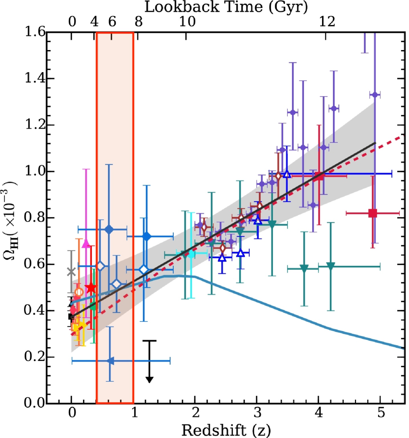
Figure 1: Cosmic H i gas density $\Omega_{\rm HI}$ as a function of redshift (top axis) and lookback time (bottom axis), adapted from rhee18. This plot uses both Ly$\alpha$ absorbers and 21-cm emission at lower-z. The redshift range observed in the FLASH survey is shown by light red shading. Further details on the observational data points used for this plot, as well as relevant references, are provided in Figure 14 of rhee18.

In a targeted search with the Arecibo telescope using pre-selection based on Mg ii absorption, briggs1983 detected two H i lines from their sample of 18 Mg ii systems at $0.36<z<1.94$. They found no correlation between Mg ii equivalent width and H i optical depth, and suggested that the lack of an observed correlation between the optical and radio absorption properties was related to the multi-component nature of the absorbing gas.

kanekar2014a used the GBT to search for 21 cm H i absorption at the redshift of 22 known quasar DLA systems with $0.8<z<3.5$ and made three detections. By combining the 21 cm and optical DLA data, these authors were able to derive spin temperatures (or lower limits) for each system. They found statistically-significant evidence for an increase in the spin temperature of DLA systems at higher redshift.

Targeted searches with radio interferometers, mainly using Mg ii pre-selection lane98; lane2001; york07; gupta2012; kanekar2014a; dutta2020 have also produced a small number of intervening 21 cm detections.

1.3 Surveys for associated 21 cm H i absorption

The detection of cold gas within the host galaxies of radio-loud AGN can provide unique insights into the distribution and kinematics of gas in the nuclear regions of active galaxies and the role gas may play in the evolution of AGN. In particular, the radio jets in these systems may drive rapid outflows of neutral gas (Morganti2005; morganti2016; scnulz2021, e.g.).

morganti2018 provide an overview of “associated H i absorption”, which arises from H i located in and around the host galaxy of a radio source. Previous searches for associated 21 cm absorption lines have generally used a known optical redshift to target a specific radio frequency. RFI limitations mean that most of these searches have been carried out at low redshift, though some higher-redshift lines have also been detected.

Large and sensitive searches for associated H i absorption in nearby radio galaxies have been carried out by gereb2014 and maccagni2017, with detection rates of up to 30%. Similar studies at higher redshifts include those by murthy2022, aditya18, aditya2019, and chowdhury2020.

The results so far suggest that the detection rate of associated H i absorption lines is higher in compact radio sources than in extended sources vermeulen2003; gupta16, and appears to be lower at redshift $z>0.5$ than in nearby galaxies aditya18; su2022; aditya2024. curran2012 postulate that there is a critical UV continuum luminosity of L${}_{\rm 1216}\sim 10^{23}$ W Hz^-1 above which neutral hydrogen is completely ionised and 21 cm absorption is no longer detected. They suggest that this may partly account for the lower H i detection rate at higher redshifts where powerful radio-loud quasars are more common. More recently, murthy2022 investigated selected targets where the UV luminosity fell below the threshold of 10²³ W Hz^-1, finding that neither UV nor radio luminosity of the AGNs is likely to cause the lower detection rate. This work suggests that the lower detection rate of associated H i 21 cm absorption lines at high redshifts may be due to evolution in the physical conditions of H i, possibly either lower H i column densities or higher spin temperatures in high-$z$ AGN environment. There have also been studies of associated absorption in Ly$\alpha$, i.e. the proximate DLAs (PDLAs), which do indeed seem to be more common towards radio selected QSOs (ellison2002; ellison2010; russell2006, e.g.).

1.4 H i absorption studies with SKA precursor telescopes

A new parameter space for H i absorption studies has recently been opened up by the development of wide-band correlators for radio interferometers that provide instantaneous redshift coverage approaching that of optical spectrographs, and by the construction of the SKA precursor telescopes ASKAP johnston2008; hotan21 and MeerKAT jonas2009 on radio-quiet sites where RFI contamination is minimised. Importantly, these radio-quiet sites uniquely allow near-continuous coverage of the 21 cm line at frequencies between 0.5 and 1 GHz, enabling spectral-line studies of H i at $0.4<z<1.8$ (allison2017; deka2023, e.g.).

The MeerKAT Absorption-Line Survey (gupta16, MALS;) is currently carrying out a search for H i absorption lines at redshift $0<z<1.45$ in several hundred fields (each of area $\sim 1\,{\rm deg}^{2}$, the total sky coverage of $\sim 1000\,{\rm deg}^{2}$) centred on bright radio-loud quasars with a known optical redshift gupta2022. This survey is optimised for lines with low H i column densities, reaching limits as low as N${}_{\rm HI}\sim 10^{19}$ cm^-2 for the brightest background sources and N${}_{\rm HI}\sim{\rm a\,few\,times}10^{21}$ cm^-2 for the other sources in general.

The wide (36 deg²) field of view, broad spectral coverage and radio-quiet site of the Australian SKA Pathfinder (ASKAP) radio telescope hotan21 makes it possible to carry out the first ‘all-sky’ survey for 21 cm H i absorption across a wide redshift range ($0<z<1.0$) without any optical pre-selection of targets. The design and science goals for such a survey, the ASKAP First Large Absorption Survey in H i (FLASH) are described in detail in the survey design paper by allison22. In contrast to the Meerkat MALS survey, FLASH is optimised for the detection of high column-density H i absorption lines (typically with N${}_{\rm HI}>10^{21}$ cm^-2) against relatively faint radio sources.

The first H i absorption-line searches with ASKAP allison15; moss17; glowacki19; sadler20; mahony2022 used a smaller array of 6–12 ASKAP dishes with a single bright continuum source placed near the field centre. These observations detected a variety of associated and intervening H i absorption lines, and showed that ASKAP can produce high-quality radio spectra that are essentially free of terrestrial RFI in the 700–1000 MHz band.

allison20 presented the first detection of H i absorption against a source away from the field centre in a wide-field ASKAP observation with 12-14 dishes (the GAMA 23 Early Science field). Like the earlier ASKAP observations, the GAMA23 data were processed with a custom data pipeline based around the Miriad software package sault95. The much larger datasets produced by the full 36-dish ASKAP array require the use of a dedicated observatory-built data pipeline, ASKAPsoft wieringa20, and so a key aim of the ASKAP Pilot Survey program was to test and verify this pipeline.

The huge size of the ASKAP spectral-line datasets means that spectral-line visibilities cannot be stored once the data have been processed through ASKAPsoft hotan21, so re-processing of the raw data is not possible. Testing and verification of the full ASKAPsoft data pipeline for FLASH data is therefore essential, and this was achieved through the ASKAP Pilot Survey program described in this paper.

1.5 Outline of this paper

Section 2 of this paper describes the two ASKAP FLASH pilot surveys carried out from 2019–22, which together covered around 3,000 deg² of sky. Section 3 gives details of the fields observed, Section 4 describes the data processing and Section 5 discusses the data products released through the CSIRO ASKAP Data Archive (CASDA). Section 6 briefly describes the continuum images and catalogues released from the pilot surveys, while Section 7 discusses the overall quality of the processed spectral-line data released in CASDA.

Section 8 presents the results from the FLASHfinder, an automated tool to search for H i absorption and discusses machine learning classifications of the detected lines. A Discussion section, an outline of future work, and a brief summary can be found in Sections 9 and 10. Some further technical details are included in the Appendices, and plots of the detected H i lines are shown in C.

2 The ASKAP-FLASH Pilot Surveys

A program of ASKAP pilot surveys was carried out before the start of the full set of five-year ASKAP surveys. Along with other ASKAP Survey Science teams, the FLASH team was allocated 100 hours of observing time for a first round of pilot surveys in 2019–20 and a further 100 hours for the second pilot survey round in 2021–22.

2.1 FLASH survey strategy and data pipeline

The FLASH pilot surveys had two main goals: to test and validate the observing and data processing strategies for the full all-sky FLASH survey, and to provide a first look at the population of H i absorption systems detected in a wide-field radio absorption-line survey conducted without any optical pre-selection.

In the pilot surveys, we carried out end-to-end tests and validation of the ASKAPsoft data pipeline to ensure that it was able to produce the required spectra, continuum images and catalogues to the quality specified in the original FLASH survey proposal as outlined by allison22. We also assessed the variation in sensitivity across the full ASKAP field of view at 711.5-999.5 MHz and measured the system performance and noise properties over a wide range in declination (from at least $+20$ deg to $-50$ deg declination) and for both daytime and nighttime observations. Figure 2 shows the sky coverage of the survey.

2.2 Choice of observing parameters

The choice of observing frequency for FLASH is a trade-off between the frequency-dependent sensitivity of the ASKAP telescope and our desire to optimize the redshift path-length for detecting H i absorption. This trade-off is discussed in detail by allison22, who show that (i) a frequency range of  711.5–999.5 MHz maximises the total absorption path length sampled, and (ii) an integration time of around two hours per field maximises the sky area that can be covered to reasonable depth in a fixed time, which in turn maximises the number of absorption lines detected and the discovery potential of the survey.

Table 1 lists the observing parameters used for the FLASH pilot survey. Individual observations used the grid of fields and pointing centres listed in Table 2 of allison22, which is designed to provide uniform sensitivity across the survey area and is the same grid used by the first RACS low survey (mcconnell2020, The Rapid ASKAP Continuum Survey;). We used the square_6$\times$6 ASKAP beam footprint hotan21 shown in Figure 3. In the frequency range used for FLASH, this provides an rms spectral-line noise that is uniform across the central 6.4 deg $\times$6.4 deg of the ASKAP field of view, as also shown in Figure 3.

Table 1: Observing parameters for the FLASH Pilot Surveys. For a detailed description of the ASKAP array, see hotan21.

Number of antennas	36 (diameter = 12 m)
Frequency range	711.5–999.5 MHz
Central frequency	855.5 MHz
Redshift coverage	$z=0.42-1.00$ (H i line)
	$z=0.67-1.34$ (OH 1665-67 lines)
Footprint	square_6$\times$6
Interleaving	None
Field of view	$6.4\times 6.4$ deg2
Integration time	2 hr (standard)
	6 hr (deep GAMA fields)
Channel width	18.5 kHz
Noise level of spectra	5.5 mJy b-1(see Figure 7)
Spatial resolution of continuum	15 arcsec

Figure 2: FLASH Pilot Survey Sky Coverage. Orange squares show the Pilot Survey 1 fields, and green squares the Pilot Survey 2 fields. Fields observed in both Pilot 1 and 2 are marked with star symbols. The coordinates are equatorial, with right ascension versus declination. The footprints of multi-wavelength surveys, such as BOSS, DES, MRC 1Jy, Stripe 82, WiggleZ, VIKING, and SPT-SZ, are included.

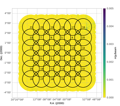
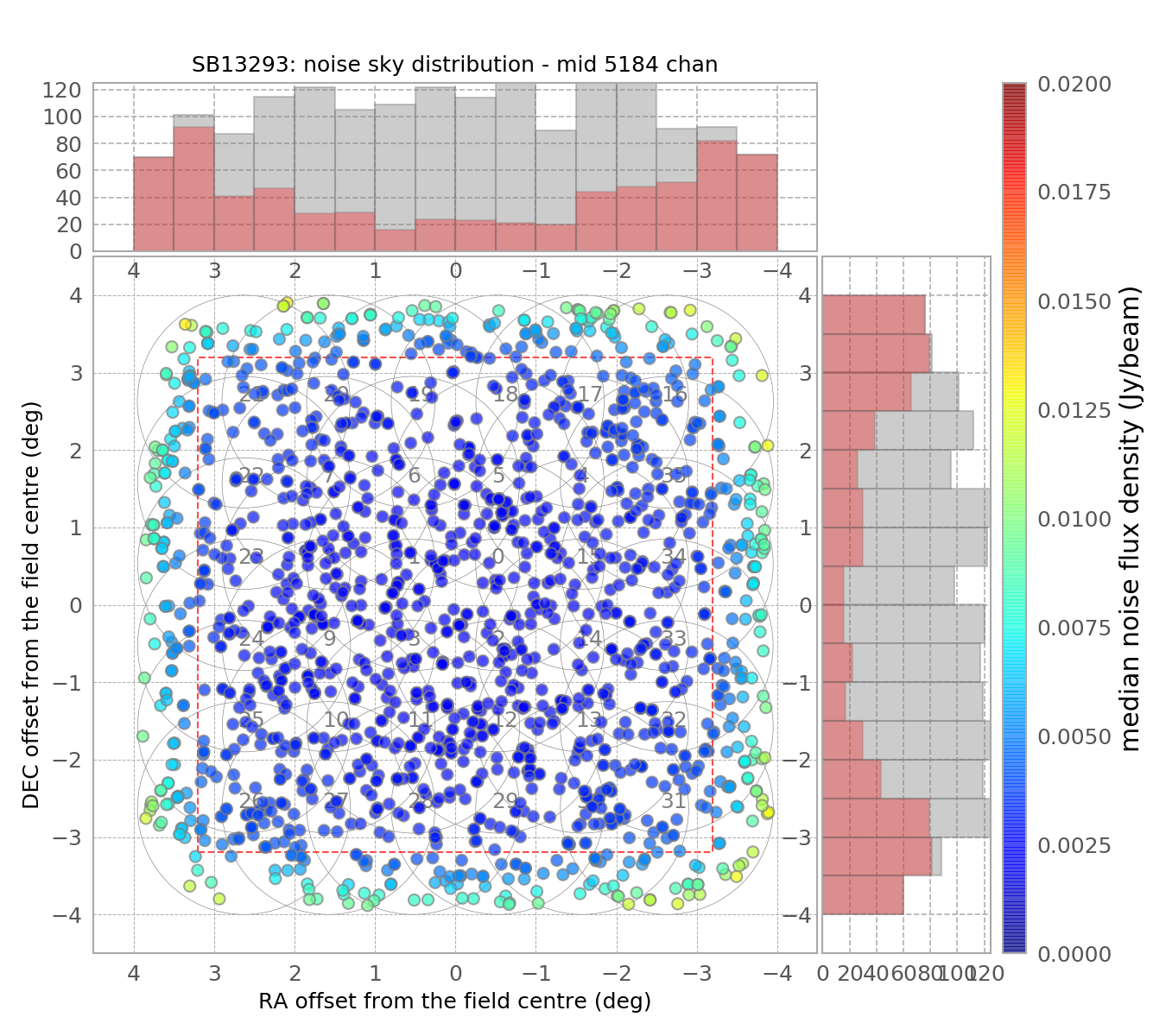
Figure 3: FLASH field of view and noise properties: (left) a FLASH continuum image showing the position of the 36 ASKAP beams in the square_6$\times$6 foootprint used to form the image, (right) measurements of spectral-line noise for extracted spectra in a 6-hour Pilot 1 observation (SBID 13293), showing that the noise is roughly uniform within a central square of 6.4 deg$\times$6.4 deg on the sky (total area 40.9 deg²). The grey histogram represents the total number of radio sources per bin, while the red histogram indicates the number of sources located beyond 3.2 degrees from the field centre, showing the increased noise at the edges of the field.

2.3 Spectral-line beamforming intervals with ASKAP

ASKAP’s Phased Array Feeds allow us to digitally form up to 36 beams across the field of view. By default, the beam-forming weights are calculated in 1 MHz intervals across the full 288 MHz bandwidth (see hotan21 for further details). At the redshifts covered by the FLASH survey this corresponds to velocity widths of 235–420 km s^-1 which would severely limit our ability to detect broader H i absorption lines.

To overcome this, the Pilot Survey observations tested a mode in which the beam-forming weights were fixed over larger bandwidths. Due to constraints in the beam-forming software only odd-numbered beam-forming intervals were possible. For this reason, tests using both 5 MHz and 9 MHz intervals were used during Pilot Survey 1. During this process, 5 MHz intervals were found to be more reliable and were subsequently used for all Pilot Survey 2 observations. The majority of Pilot 1 fields used 9 MHz beamforming intervals with the exception of SBIDs (Scheduling block IDs) 10849, 10850, 11051, 11052, 11053, 11068 which used 5 MHz intervals.

3 Observations

Tables 2 and 3 list the fields observed in the first and second pilot surveys. Some further information on individual observations (including measurements of the rms noise and a quality assessment) is included in the tables in Appendix 4.

3.1 Pilot Survey 1: 2019-20

The first FLASH pilot survey, covering $\sim 1500$ deg² of sky was carried out with the full 36-dish ASKAP telescope between December 2019 and September 2020. The 37 2-hr fields and four 6-hr fields were successfully processed through the ASKAPsoft data pipeline are shown in Figure 2 and listed in Table 2. These fields were chosen to span a wide range in declination, but also to include some areas of sky with good quality optical data, notably the three equatorial GAMA driver11 fields.

In the first pilot survey, we observed 40 fields with an integration time of two hours each (the 2-hr fields). For six of these fields, we also carried out a longer (6 hr) integration (the 6-hr fields).

Of the 40 2-hr fields, 37 were successfully processed and have been released in CASDA. One of these fields (listed as J2022-2507P in Table A1) was observed at the wrong RA because of a scheduling error, but still contains useful data. A further three fields were observed in July 2020 but could not be processed at the time because of computing limitations. These fields may be processed in the future if resources permit.

Of the six 6-hr fields observed in the first pilot survey, only four were successfully processed and have been released in CASDA. The data pipeline failed at the processing stage for two of the 6-hr fields (G12B_long and G15B_long) due to errors in the data, and no processed data are available for these fields. One further 6-hr field (G09B_long, SBID 11068) was successfully processed but only the region with $z>0.82$ could be recovered in post-processing (see Section 4).

3.2 Pilot Survey 2: 2021-22

After some further refinements to the data processing pipeline, a second pilot survey, covering a further $\sim 2000$ deg² of sky, was carried out from November 2021 to August 2022. The fields observed in this second pilot survey are also shown in Figure 2, and are listed in Table 3.

In the second pilot survey, we observed 50 fields with an integration time of two hours each. Four of these were repeats of fields observed in Pilot 1 (Fields 122, 123, 160, 306), and eight further Pilot 2 fields overlapped with the GAMA equatorial fields observed in Pilot 1 (Fields 545, 546, 547, 553, 554, 559, 560, 561). These repeat fields were used to test the reliability and reproducibility of absorption lines detected by ASKAP, as discussed in Section 8.7.

Many of the Pilot Survey 2 fields were chosen to overlap with large-area surveys for which optical data are available, in particular SDSS Stripe 82 hodge11; annis14; jiang14, the MRC 1-Jy Survey mccarthy1996 and the WiggleZ galaxy redshift survey drinkwater18.

3.3 Sky coverage of the two Pilot Surveys

The fields released in CASDA from the first pilot survey cover roughly 1000 deg² of sky and represent 90 hours of ASKAP observing time. The 50 fields observed in the second pilot survey cover around 2000 deg² of sky. Together, the data released in CASDA from the two FLASH pilot surveys comprise 77 unique ASKAP fields with a total sky coverage of around 3080 square degrees. Seventeen of these fields were observed two or more times. In four cases, a field observed in Pilot 1 was re-observed in Pilot 2 for validation purposes, including consistency checks on the observed properties and the linefinder results. For the other 13 fields, the observations made in Pilot 2 were mainly repeated in an attempt to improve the data quality of fields that showed spectral-line artefacts (see Section 7.2).

3.4 The GAMA 9h, 12h and 15h fields

We chose to include the three equatorial fields (at 9h, 12h and 15h RA) from the GAMA galaxy survey driver11 in the first pilot survey. Each of the optical GAMA fields covers 48 deg² of sky and can be covered by two ASKAP pointings. The GAMA fields were chosen because they have particularly good photometric and spectroscopic information available. In addition, ching17 have made optical identifications of many of the radio continuum sources in these GAMA fields and obtained additional optical spectra for objects not in the original GAMA catalogue.

The GAMA fields were observed on non-standard field centres in the first pilot survey, so that each GAMA field could be completely covered by two ASKAP pointings su2022. In the second pilot survey, the GAMA fields were re-observed on the standard FLASH pointing centres listed by allison22.

3.5 SDSS Stripe 82 fields

SDSS Stripe 82 annis14 is a well-studied 300 deg² region of sky with RA in the range 20h to 04h (300 to 60 deg) and declination between -1.26 and +1.26 deg. This strip of sky was repeatedly scanned (70-90 times) by the SDSS imaging survey in $ugriz$ filters and has been the focus of many studies of transient and variable objects. The available multi-wavelength data products include deep optical jiang14 and 1.4 GHz radio imaging hodge11 as well as extensive optical spectroscopy.

The Stripe 82 area is fully covered by a set of 20 FLASH fields (fields $525-534$ and $573-582$ inclusive) observed during the second pilot survey (see the Notes section of Table 3). Unfortunately, many of these Stripe 82 pilot observations have spectral artefacts and should be used with caution (see Section 7.2 for more details). These observations will be repeated during the full five-year FLASH survey.

3.6 WiggleZ fields

The FLASH Pilot Survey also overlaps part of the WiggleZ redshift survey drinkwater18 area. WiggleZ targeted a UV-selected galaxy sample of candidate star-forming galaxies at redshift $0.2<z<1.0$ across several fields covering a total of $\sim 1000$ deg² of sky, so is well-matched to the redshift range covered by FLASH. Further analysis will be provided by Eden at al. 2024 submitted.

Table 2: Log of observations for the first FLASH Pilot Survey; (1) FLASH field name; (2) Scheduling block ID; (3) Right Ascension (hhmmss.ss); (4) Declination (ddmmss.s); (5) Observation date (dd-mm-yy); (6) Integration time in hrs. The GAMA fields were observed using different pointing centres from the standard FLASH pointing grid listed in Table 2 of allison22, as was field J2022-2507P (SBID 13296). The full table is provided in the Appendix.

Field	SBID	RA_2000	Dec_2000	Date	t (h)
(1)	(2)	(3)	(4)	(5)	(6)
F302P	10850	00 00 00.15	$-$25 07 52.2	17-Dec-19	2
F088P	13299	00 21 10.59	$-56$ 18 22.7	20-Apr-20	2
F303P	11053	00 27 10.19	$-25$ 07 47.2	05-Jan-20	2
F123P	13290	00 36 55.38	$-50$ 05 45.3	19-Apr-20	2
F304P	13291	00 54 20.38	$-$25 07 47.2	19-Apr-20	2
F089P	13298	01 03 31.76	$-$56 18 22.7	20-Apr-20	2
F306P	13281	01 48 40.75	$-$25 07 47.2	18-Apr-20	2
F165P	15213	02 13 57 39	$-$43 52 35.4	04-Jul-20	2
F307P	13268	02 15 50.94	$-$25 07 47.2	17-Apr-20	2
F308P	15212	02 43 01.13	$-$25 07 47.2	04-Jul-20	2
F309P	13269	03 10 11.32	$-$25 07 47.2	17-Apr-20	2
F170P	15215	05 01 23.72	$-$43 52 35.4	05-Jul-20	2
F718P	13270	08 43 38.18	$+$18 51 28.9	17-Apr-20	2
F719P	13271	09 09 49.09	$+$18 51 28.9	17-Apr-20	2
F607P	13284	10 08 16.55	$+$06 17 42.1	18-Apr-20	2
F608P	13272	10 33 06.21	$+$06 17 42.1	17-Apr-20	2
F550P	13305	10 33 06.21	$+$00 00 00.0	20-Apr-20	2
F194P	15208	18 25 06.98	$-$43 52 35.4	04-Jul-20	2
F195P	15229	18 58 36.47	$-$43 52 35.4	05-Jul-20	2
F197P	15209	20 05 34.88	$-$43 52 35.4	04-Jul-20	2
J2022-2507P	13372	20 22 38.64	$-$25 07 47.2	22-Apr-20	2
F198P	15230	20 39 04 47	$-$43 52 35.4	05-Jul-20	2
F199P	15211	21 12 33 67	$-$43 52 35.4	04-Jul-20	2
F351P	10849	22 11 19.25	$-$25 07 47.2	17-Dec-19	2
F352P	11051	22 38 29.43	$-$25 07 47.2	05-Jan-20	2
F159P	13278	22 46 09.23	$-$50 05 45.3	17-Apr-20	2
F120P	13297	22 56 28.24	$-$56 18 22.7	20-Apr-20	2
F353P	11052	23 05 39.62	$-$25 07 47.2	05-Jan-20	2
F160P	15873	23 23 04.62	$-$50 05 45.3	04-Sep-20	2
F354P	13279	23 32 49.81	$-$25 07 47.2	18-Apr-20	2
F121P	13296	23 38 49.41	$-$56 18 22.7	19-Apr-20	2
Fields in the GAMA survey area
FG9A	13285	08 47 35.59	$+$00 30 00.0	18-Apr-20	2
FG9A_long	13293	08 47 35.59	$+$00 30 00.0	19-Apr-20	6
FG9B	13283	09 12 25.24	$+$00 30 00.0	18-Apr-20	2
FG9B_long	11068	09 12 25.24	$+$00 30 00.0	07-Jan-20	6
FG12A	13334	11 47 35.17	$-$00 30 00.0	21-Apr-20	2
FG12A_long	13306	11 47 35.17	$-$00 30 00.0	20-Apr-20	6
FG12B	13335	12 12 24.83	$-$00 30 00.0	21-Apr-20	2
FG15A	13336	14 16 33.10	$+$00 30 00.0	21-Apr-20	2
FG15A_long	13294	14 16 33.10	$+$00 30 00.0	19-Apr-20	6
FG15B	13273	14 41 22.76	$+$00 30 00.0	17-Apr-20	2

Table 3: Observation log for the second FLASH Pilot Survey. Fields with repeat observations are marked by ^∗, Cols (1)–(6) are the same as in Table 2, Col (7) lists SDSS Stripe 82 (S82), Pilot 1 repeats (R), and GAMA fields (G).

Field	SBID	RA_2000	Dec_2000	Date	t (h)	Notes
(1)	(2)	(3)	(4)	(5)	(6)	(7)
F122	34941	00 00 00.00	$-$50 05 45.2	29-Dec-21	2
F525∗	34581/42299	00 12 24.80	+00 00 00.0	20-Dec-21/08-July-22	2	S82
F123	37448	00 36 55.30	$-$50 05 45.2	18-Feb-22	2	R
F526∗	34783/42275	00 37 14.40	$+$00 00 00.0	26-Dec-21/07-Jul-22	2	S82
F527∗	34568/42300	01 02 04.14	$+$00 00 00.0	19-Dec-21/08-Jul-22	2	S82
F305	37449	01 21 30.50	$-$25 07 47.2	18-Feb-22	2
F528	37450	01 26 53.70	$+$00 00 00.0	18-Feb-22	2	S82
F529	34557	01 51 43.40	$+$00 00 00.0	18-Dec-21	2	S82
F306	37475	01 48 40.70	$-$25 07 47.2	19-Feb-22	2	R
F255∗	35939/41148/41226	01 52 56.40	$-$31 23 14.7	15-Jan-22/01-Jun-22/03-Jun-22	2
F530	37431	02 16 33.10	$+$00 00 00.0	17-Feb-22	2	S82
F256	34584	02 21 10.50	$-$31 23 14.7	20-Dec-21	2
F531	34546	02 41 22.70	$+$00 00 00.0	17-Dec-21	2	S82
F257	37451	02 49 24.70	$-$31 23 14.7	18-Feb-22	2
F532	34569	03 06 12.40	$+$00 00 00.0	19-Dec-21	2	S82
F258	37452	03 17 38.80	$-$31 23 14.7	18-Feb-22	2
F533∗	35943/42278	03 31 02.07	+00 00 00.0	15-Jan-22/08-Jul-22	2	S82
F310	37432	03 37 21.50	$-$25 07 47.2	17-Feb-22	2
F534	34558	03 55 51.70	+00 00 00.0	18-Dec-21	2	S82
F311	37453	04 04 31.70	$-$25 07 47.2	18-Feb-22	2
F312	37797	04 31 41.80	$-$25 07 47.2	02-Mar-22	2
F313	34547	04 58 52.00	$-$25 07 47.2	17-Dec-21	2
F314∗	34570/41061/41065	05 26 02.26	$-$25 07 47.2	19-Dec-21/29-May-22/29-May-22	2
F545	34548	08 28 57.90	+00 00 00.0	17-Dec-21	2	G
F546	34559	08 53 47.50	+00 00 00.0	18-Dec-21	2	G
F547	34549	09 18 37.20	+00 00 00.0	17-Dec-21	2	G
F377	34571	09 36 00.00	$-$18 51 45.4	19-Dec-21	2
F719∗	34560/41066/41084	09 09 49.00	$+$18 51 28.8	18-Dec-21/29-May-22/30-May-22	2	R
F378	34561	10 02 10.90	$-$18 51 45.4	18-Dec-21	2
F553	34572	11 47 35.10	+00 00 00.0	19-Dec-21	2	G
F554	34917	12 12 24.80	+00 00 00.0	28-Dec-21	2	G
F555	34562	12 37 14.40	+00 00 00.0	19-Dec-21	2
F559∗	34551/41068/41085	14 16 33.10	+00 00 00.0	18-Dec-21/29-May-22/30-May-22	2	G
F560	34563	14 41 22.70	+00 00 00.0	19-Dec-21	2	G
F561	34576	15 06 12.40	+00 00 00.0	20-Dec-21	2	G
F011	34564	16 45 52.80	$-$80 02 36.7	19-Dec-21	2
F287	34552	16 56 28.20	$-$31 23 14.7	18-Dec-21	2
F151	34553	17 50 46.10	$-$50 05 45.2	18-Dec-21	2
F398∗	33616/41050/41071	18 45 49.00	$-$18 51 45.4	17-Nov-21/28-May-22/29-May-22	2
F573	34554	20 04 08.00	+00 00 00.0	18-Dec-21	2	S82
F574	34565	20 28 57.90	+00 00 00.0	19-Dec-21	2	S82
F575	34577	20 53 47.50	+00 00 00.0	20-Dec-21	2	S82
F576	34578	21 18 37.20	+00 00 00.0	20-Dec-21	2	S82
F577∗	34555/42296	21 43 26.90	+00 00 00.0	18-Dec-21/08-Jul-22	2	S82
F578∗	34580/42297/43424	22 08 16.50	+00 00 00.0	20-Dec-21/08-Jul-22/14-Aug-22	2	S82
F579∗	34597/42298	22 33 06.00	+00 00 00.0	21-Dec-21/08-Jul-22	2	S82
F580	34567	22 57 55.80	+00 00 00.0	19-Dec-21	2	S82
F160∗	34939/42323/43426	23 23 04.62	$-$50 05 45.2	29-Dec-21/09-Jul-22/14-Aug-22	2	R
F581∗	34781/41072/41105/41184/41225	23 22 45.50	+00 00 00.0	26-Dec-21/23-Jun-22/04-Jul-22/04-Jul-22/04-Jul-22	2	S82
F582	34556	23 47 35.10	+00 00 00.0	18-Dec-21	2	S82

4 Data Processing

4.1 Pipeline processing

The observations were processed through the standard ASKAPsoft pipeline whiting2020. This is a scripted workflow that, for FLASH pilot processing, ran on the galaxy supercomputer at the Pawsey Supercomputing Centre. It performs all the necessary calibration, imaging and source-extraction tasks required to produce science-ready data products. A detailed description of the pipeline can be found elsewhere, but we give specific details relevant for the FLASH processing here.

The bandpass and primary flux calibration were done using PKS B1934$-$638, which was observed at the centre of each beam for $\sim 200$ sec. The bandpass solutions were derived for each beam, antenna, polarisation combination and smoothed over intervals of 1 MHz to improve the signal-to-noise of the calibration solutions. Each beam of the science observation was calibrated with the solutions from the corresponding beam of the bandpass observation.

All imaging of the science observations was done independently for each beam. A continuum image (using visibilities averaged to 1 MHz resolution) was made first, through an iterative self-calibration approach. This involves imaging, then calibrating the time-dependent complex gains against a model derived from the image, then re-imaging (with more cleaning) after applying those gain solutions. The imaging used multi-scale (scales of 0, 6, 15, 30, 45, 60 pixels) multi-frequency (2 Taylor-terms) synthesis, with Wiener preconditioning applied using robustness=0.0. This gives an average PSF size (averaged over all Pilot observations) of $18\times 13$ arcsec. A second image was also made with a robustness=1.0 (giving an average resolution of $28\times 20$ arcsec) to more closely match the spatial resolution of the spectral line cube.

The full-spectral resolution data were then imaged over the full band. First, the continuum was subtracted from the visibilities by forming a model from the continuum image and transforming to the ($u,v$) plane. After this, the data were imaged in each channel to form a spectral cube. Two cuts on the ($u,v$) distance were applied, by removing baselines $<70$m to limit solar interference, and $>4000$m to limit the size of the full image. Multi-scale imaging (scales 0, 3, 10, 30 pixels) was done, using Wiener preconditioning with robustness=1.0 – this, in addition to the ($u,v$) cuts, provides an average PSF resolution in the middle of the band of $29\times 22$ arcsec, ranging from $34\times 36$ arcsec to $25\times 19$ arcsec across the band. Following imaging, a further round of continuum-subtraction was then applied, to further remove any continuum residuals. Each spectrum in the cube (that is, each spatial pixel) had the continuum level fitted within each beam-forming interval (or, in the case of Pilot Phase 1, each 1 MHz interval) and subtracted. Breaking at the edge of each beamforming interval allows the removal of any residual discontinuities not completely removed by the bandpass calibration (this is particularly important for brighter sources that might have a higher signal-to-noise than we get on B1934$-$638 in 200 sec).

The continuum (1 MHz-resolution) data were also imaged in each channel to form continuum cubes. For Pilot 2 these were done with the same ($u,v$) cuts and preconditioning as the spectral cubes, to provide matching-resolution data to enable more accurate extraction of continuum spectra in post-processing.

Once imaging was complete, the individual beams were mosaicked together to form the full field images in each of continuum, continuum-cube and spectral-cube modes. Source-finding was run with Selavy whiting2012 to create catalogues of continuum components and islands, and the full-spectral-resolution spectra at the location of each component brighter than 45 mJy (20 mJy for the 6-hour observations) were extracted and stored as 1-dimensional spectra.

4.2 Pilot 1 data and post-processing

Observations for the first FLASH pilot survey were carried out with 5 or 9 MHz beam-forming intervals, rather than the standard 1 MHz intervals used in most ASKAP observations. It was discovered early on during the data processing of the first pilot survey that these larger beam-forming intervals were not being implemented as anticipated, with large jumps in amplitude and phase evident on 1 MHz intervals.

As these jumps occurred precisely at the 1 MHz boundaries, they could be corrected for in the pipeline processing by smoothing the bandpass solutions on 1 MHz intervals as well as removing any residual artefacts by using 1 MHz intervals for the image-based continuum subtraction. This procedure corrects for the large amplitude jumps and leads to a clean, smooth bandpass across the entire band. However, 1 MHz corresponds to a line width of approximately 300 km s^-1 at these redshifts, meaning that processing the data using 1 MHz intervals risks removing any real H i absorption signatures of similar line widths. This could mean that some H i absorption lines are either completely subtracted out or (if detected) the shape of the line is significantly altered because of the limited line-free channels used for the continuum subtraction in each 1 MHz interval.

To address this issue, we carried out some further post-processing outside of the ASKAPsoft pipeline. This involved downloading the spectral cubes from CASDA that were made prior to the image-based continuum subtraction, and extracting the spectra towards all bright radio sources. For the majority of the fields observed the flux limit for spectrum extraction was set at 30 mJy, which is deeper than the pipeline limit of 45 mJy. For the longer 6 hr integrations, a flux density threshold of 10 mJy was used. A spectrum was extracted at the peak pixel of each catalogued continuum component.

After extracting the spectra from the spectral cube, some further continuum subtraction was carried out to remove any residual continuum not subtracted in the visibility domain. This involved fitting a second-order polynomial within each 5 or 9 MHz beam-forming interval, while masking any strong lines (either due to real absorption or RFI) that were more than 3-$\sigma$ above the noise.

This post-processing procedure allowed us to recover some H i absorption lines that were inadvertently subtracted out by using the default pipeline processing parameters, but did lead to some broader spectral ripples in some frequency ranges, particularly towards the brighter continuum sources. Figure 4 shows an example of a broad H i absorption line that was subtracted out in the initial processing, but was recovered after re-doing the continuum subtraction over wider frequency intervals. The post-processed data will be publicly released in CASDA alongside this publication.

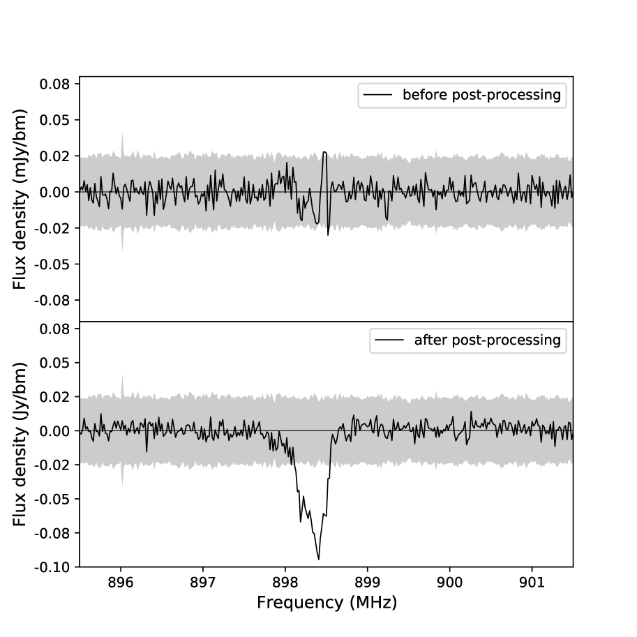
Figure 4: An example of a broad H i absorption line detected after post-processing of the FLASH pilot survey data. The spectrum was extracted toward PKS 2311-477 in FLASH 160P field (SB 15873 component 5a, $S=1.04$ Jy). The grey shade is set at five times the rms spectral-line noise. The absorption is found at $z=0.5811$, and the FWHM linewidth from a single Gaussian fit is 112 km s^-1.

4.3 Pilot 2 data

The overall data processing method for Pilot Survey 2 was similar to that for Pilot 1. Improvements in correctly implementing larger beam-forming intervals were made prior to the Pilot 2 survey, meaning that 5-MHz intervals were used for all Pilot-2 survey observations and post-processing of the data was not required.

Unfortunately, over half of the Pilot 2 fields show significant ripples (‘wobbles’) in their spectra, caused by a processing error in the bandpass calibration for a large batch of observations made between 17 December 2021 and 15 January 2022 (see Section 7.2 for more details). These wobbles are particularly noticeable in the spectra of bright sources, and the features occur across the whole frequency band.

Although 24 of the SBIDs with spectral wobbles were re-observed after February 2022, more than half of these repeated fields were affected by tropospheric ducting of RFI (see Section 7.2) that affected at least 20% of the frequency range. These fields will be repeated in the full FLASH survey.

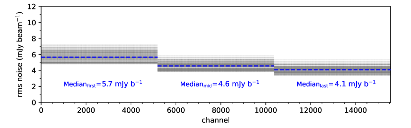
Figure 5: Measurements of median spectral-line noise (in mJy beam^-1 ch^-1; channel width: 18.5 kHz) in three sub-bands of FLASH field 307 (SBID 13268), showing the values in three sub-bands within the 712-1000 MHz observing band. Grey lines show the values for individual sources within 3.2 degrees of the field centre, and the dashed blue line shows the median for the field as a whole.

5 Data products released in CASDA

5.1 Processed data products

Processed data products from the FLASH pilot surveys have been released through the CSIRO ASKAP Science Data Archive (CASDA) at https://research.csiro.au/casda/ under project code AS 109. To download data, users need to register and create a CASDA account.

The output data products loaded into CASDA for each observation are listed with the examples of the filenames as follows:

1. Continuum catalogues: A component catalogue and a separate island catalogue are produced by the Selavy source finder whiting2012. These catalogues are used for data validation, and the component catalogue positions are also used to extract spectra for the absorption-line search. The island catalogues provide a useful resource for optical cross-matching.
   $-$ File examples: “selavy-image.i.SB15873.cont.taylor.0.
    restored.conv.components.xml”, “selavy-image.i.SB15873.
    cont.taylor.0.restored.conv.islands.xml”

2. Continuum images and cubes: We produce both a Stokes I continuum image at $\sim 15$ arcsec resolution (rms noise $\sim 90\,\mu$Jy/beam) and a continuum cube. The continum cubes are matched to the 30 arcsec resolution of the spectral-line cube for the later Pilot fields.
   $-$ File examples: “image.i.SB15873.cont.taylor.0.restored.
    conv.fits”, “image.restored.i.SB15873.contcube.conv.fits”

3. Spectral-line cubes: Two full spectral-line cubes are produced for each SBID. An initial spectral cube is created after continuum subtraction in the visibility domain, and a final spectral cube after the image-based continuum subtraction. This second cube is used to extract the individual H i  spectra. Both cubes cover the full 288 MHz bandwidth at 18.5 kHz spectral resolution with all 36 beams mosaiced together to produce a single cube of the full ASKAP field.
   $-$ File examples: “image.restored.i.SB15873.cube.contsub.fits”

4. Individual spectra at positions of continuum sources: The ASKAPsoft pipeline extracts individual source and noise spectra for all radio components with flux densities above 45 mJy/beam. The spectra can be downloaded individually, or as a bulk .tar file for each SBID.
   $-$ File examples: “spec$\_$SB15873$\_$component_1a.fits”

5. Validation reports: These reports include metrics and general notes on data quality.

5.2 Data validation and quality assessment

The processed data products from the ASKAPsoft pipeline are assessed and validated by the FLASH science team before their public release. This data validation uses a checklist that takes into account the metrics provided by the ASKAPsoft pipeline (such as measurements of the rms noise in line and continuum), as well as a visual inspection of the images and a representative sample of spectra by members of the science team.

The completed checklist provides a numerical score, which the team use to classify each SBID as ‘Good’, ‘Uncertain’ or ‘Bad’. SBIDs classified as Good or Uncertain are released, but those classified as Bad remain unreleased and are flagged for reobservation. The team also provide some brief Release Notes to accompany the CASDA data.

5.2.1 Continuum data validation

The validation data provided in CASDA for the continuum images include beam diagnostics, the spatial distribution of identified sources, an measurement of the rms noise in the continuum, and a flux density comparison with other surveys (NVSS, SUMSS or RACS). Astrometric checks are also carried out by measuring the median position offset from published surveys.

As part of the data validation process, the FLASH team checked that the continuum catalogues were present and contained a reasonable number of sources, typically between 10,000 and 20,000. We also visually inspected each continuum image to ensure that there were no obvious problems such as large-scale patterns or artefacts around strong sources.

5.2.2 Spectral-line data validation

In addition to the diagnostics provided by ASKAPsoft, the FLASH team verifies the presence of the image cubes, and the presence of several hundred spectra that are expected from each of our observations. We also measured the rms noise in the spectral line data both for the whole frequency range and across three sub-bands as shown in Figure 5, and checked that this was in line with expectations. Further details will be described in Section 7.

Figure 6: An example of a spectral-line plot produced by the FLASH team during post-processing and used in data validation. The grey band is set at five times the rms spectral-line noise, so a line that extends beyond this band will have peak S/N $>5$. The source shown here (NVSS J015516-251423, SB 37475 component 95a) has an H i absorption line at $z=0.7251$ ($f=823.4$ MHz) (see Table 6).

Finally, as part of the post-processing workflow, we produce spectral-line plots like that shown in Figure 6. The extracted spectra of the ten brightest sources in each field are then inspected to check for any artefacts or non-uniformity of the bandpass.

6 Continuum images and catalogues

6.1 Wide field continuum images

FLASH observations provide high-quality continuum products, including wide field images and source catalogues, in addition to the spectral-line data. As can be seen from Table 4, the FLASH continuum images are intermediate in sensitivity between the first epoch of RACS-Low mcconnell2020 and the EMU Pilot Survey norris2021.

Table 4: Comparison of continuum properties for images from three ASKAP surveys: FLASH, RACS-Low, and EMU.

Survey	Central	Integration	1 $\sigma$ rms	Resolution
	freq. (MHz)	time	($\mu$Jy/beam)	arcsec
RACS-Low	888	15 minutes	$\sim 250$	15
FLASH	856	2 hours	$\sim 90$	15
EMU	944	10 hours	$\sim 30$	12-15

The restored total-intensity (Stokes I) continuum images are accumulated over the entire bandwidth being processed. Within 3.2 deg from the field centre, the rms noise in the continuum images is uniform. Most continuum images are of excellent quality and revealed several radio sources with complex asymmetric morphologies.

The rms noise level in the 2-hour continuum images is typically $\sim 90\,\mu$Jy beam^-1, i.e. roughly five times deeper than NVSS (450$\mu$Jy beam^-1) and an order of magnitude deeper than SUMSS ($\sim 1$ mJy beam^-1).

6.2 Selavy radio source catalogues

As described in Section 5.1, the ASKAPsoft pipeline generates two different continuum source catalogues via the ASKAP source-finder Selavy:
(i) An island catalogue is generated first - this is a catalogue of groups of contiguous pixels that are above some detection threshold.
(ii) A component catalogue is then generated, where each component is a two-dimensional Gaussian, parameterised by a location, flux, size and orientation. Each island has one or more components fitted to it, so there is a one-to-many relationship between the island and component catalogues.
Both catalogues are available for download through CASDA.

6.3 Astrometric accuracy

The astrometric accuracy of the listed ASKAP continuum catalogues is determined by the combination of a statistical component (set by the S/N of the source and the angular resolution of the image), and a systematic component (set by the accuracy to which the measured source positions can be aligned with a standard reference frame) heywood2016. For the FLASH continuum sources of interest for this project, the statistical component is small ($<0.1$ arcsec for a 10 mJy source) and the position uncertainty is dominated by the systematic component. The size of this systematic component is estimated at the data validation stage through a cross-comparison with other large-area source catalogues. For the pilot surveys, these catalogues were NVSS Condon1998 and SUMSS Mauch2003.

The data validation reports show systematic offsets of up to 1 arcsec (and occasionally larger) in both RA and Dec for individual ASKAP fields. In this paper we adopt an indicative astrometric error of 1 arcsec for the FLASH positions, noting that hale2021 found offsets of a similar size for the ASKAP RACS-Low fields. Although we could improve the astrometric accuracy of the pilot survey positions by correcting for the known RA and Dec offsets of each SBID, we chose not to do so in this paper because the pipeline positions are accurate enough for us to be able to match our bright ($>30$ mJy) sources with published radio catalogues. We plan to revisit the ASKAP astrometry in future, in a paper that identifies and discusses the host galaxies of the H i absorption lines found in the FLASH pilot surveys.

6.4 Flux-density scale

To check the ASKAP flux density scale in the FLASH band (712–1000 MHz), we cross-matched sources in our southern (Dec $<-30^{\circ}$) pilot fields with the SUMSS catalogue Mauch2003. SUMSS was chosen because its 843 MHz survey frequency is close enough to the FLASH band centre at 856 MHz that we expect the flux densities to be directly comparable.

From a cross-matched sample of over 5000 bright ($>20$ mJy) and spatially unresolved FLASH continuum components, we find that the FLASH and SUMSS sources are on the same flux density scale to within 2–3%. Since SUMSS itself is consistent with the 1.4 GHz NVSS flux density scale Mauch2003, this gives us confidence in the reliability of the ASKAP flux density measurements.

7 Spectral-line data

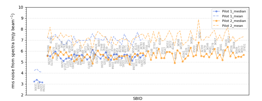
Figure 7: RMS spectral-line noise estimate measured from the noise spectra of all FLASH Pilot fields. Individual dots on the dashed and solid lines indicate the mean and median noise from the mid-5184 channels of all noise spectra in each field. 6-hr fields with lower rms levels are marked as stars.

Figure 8: RMS spectral noise comparison across different right ascension (left), declination (middle), and day/night observation (right) demonstrating uniform noise. Blue and orange crosses are from Pilot 1 and Pilot 2, respectively. 6-hr fields with lower rms levels are marked as stars.

7.1 Uniformity of the FLASH data over time

One aim of the Pilot Surveys was to check the uniformity and reproducibility of the ASKAP data. To do this, we tested for variations in sensitivity either with declination or between day-time and night-time observations.

7.1.1 Spectral-line sensitivity

Figure 7 shows the overall rms noise in the spectral-line, measured across all FLASH fields in date order. The rms noise in both continuum and spectra-line data remained roughly uniform over the period of almost three years during which the observations were carried out.

The rms noise in the extracted spectra from the 2-hour fields has a median value of 4.6 mJy per beam per channel in the central third of the frequency band (808–904 MHz) and ranges from 4.2 to 5.3 mJy beam^-1 ch^-1 in this sub-band (Figure 5). This is consistent with the range of 3.2–5.1  mJy beam^-1 ch^-1 quoted in Table 1 of allison22. The rms noise for the 6-hour fields was around 3.5 mJy per beam per channel, which is close to the value expected for the longer observing time.

The spectral-line sensitivity varies by 25–30% across the observing band because of changes in the ASKAP effective system temperature T_sys with frequency (hotan21, see Figure 22 of). Figure 5 shows this variation for a typical SBID.

7.1.2 Sensitivity versus sky position

FLASH fields are widely spread over the sky, so we were able to compare the noise across a wide range in R.A and declination, and between daytime and nightime. Figure 8 shows that the noise properties are roughly uniform with declination.

7.1.3 Daytime versus night-time observing

The right-hand plot in Figure 8 shows the rms noise as a function of local observing time (AWST). We see no significant difference in sensitivity between daytime observations and observations made at night.

7.2 Spectral-line artefacts

We identified several artefacts affecting the data quality of the spectra as shown in Figure 9. The underlying cause of three of the artefacts seen in the pilot survey data has now been addressed, and these artefacts are not expected to occur in future FLASH observations. These artefacts were:

1. Glitches at the edges of beam-forming intervals. Data from the first 18 Pilot 1 fields randomly showed glitches on 1 MHz interval due to the issues with bandpass smoothing parameterisation. This problem has been fixed, and is not seen in data taken after April 2020.

2. Correlator dropouts. These are artefacts in specific frequency ranges, caused by data dropouts in an ASKAP correlator block that were not properly accounted for in processing. The main frequency ranges affected at 915–920 MHz (corresponding to H i redshifts in the range $0.543<z<0.552$) and 987–992 MHz (H i at $0.431<z<0.439$. This problem has largely been fixed, and mainly affected data taken before 2021.

3. Wobbles. Wobble-like features are seen in the processed spectra of bright sources in almost all Pilot 2 fields observed between 17 December 2021 and 15 January 2022. These wobbles were produced during processing by the use of incorrect parameters in fitting the spectral bandpass, and affect data across the whole spectral band. Delays in uploading the processed data to the CASDA archive for data validation meant that the problem was not identified immediately, and because the ASKAP spectral-line visibilities are deleted immediately after processing it was not possible to reprocess the data with the correct parameters. The problem is not expected to recur.

There is also one ongoing effect that can produce significant spectral-line artefacts:

1. Tropospheric ducting of RFI. This occurs under particular atmospheric conditions, when radio signals from distant transmitters are refracted in the troposphere and can propagate over large distances. Ducting can occur in the ASKAP frequency range as well as at lower frequencies sokolowski2017. For FLASH observations, tropospheric ducting can result in the telescope seeing RFI from mobile phone bands used in Perth and other communities well beyond the radio-quiet zone in which ASKAP is located. When ducting is present, ducted RFI signals can occupy up to 20% of the FLASH frequency band. The frequencies most commonly affected are $758-788$ MHz, $870-890$ MHz, and $943-960$ MHz.

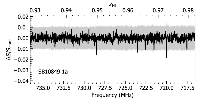
Figure 9: Examples of spectral-line artefacts seen from the Pilot data. From top to bottom, each panels presents glitches, correlator dropouts, wobbles, and tropospheric ducting of RFI in spectra.

Figure 10: Top: an example of wobbles seen in the spectra from some of the Pilot 2 fields. This spectrum is extracted toward J221238+015250 (SB 34580 1a, F $=$4.115 Jy). 20 MHz-width of the spectrum near the centre of the entire band is taken. Bottom: this field (FLASH 578) has been re-observed. The re-observed spectrum toward the same source shows a good quality (SB 43424 1a).

Ducted RFI was rarely seen in FLASH pilot survey data taken before January 2022, but became much more common, after that time. The reason for this is not yet understood, but well over half the FLASH pilot survey observations between May and August 2022 (17/24 fields) showed ducted RFI in the spectra of bright sources (see Figure 9 for an example).

If this high rate of ducting occurs again in future, we can minimize its effects in two ways. The weather conditions that give rise to tropospheric ducting can often be predicted, and we can avoid scheduling FLASH observations when these conditions are present. Alternatively, if ducting conditions are detected at the telescope while a FLASH observation is underway, the observation will be stopped, the data discarded, and the observation rescheduled for a later time. A more detailed discussion of ducting effects at the ASKAP site is given by indermuehle2018 and lourenco2024.

8 FLASHfinder - an automated search for H i absorption lines

8.1 An automated absorption line-finder for ASKAP

The FLASHfinder Bayesian line-finding tool allison12 was designed to identify and parameterise H i absorption lines in large ASKAP spectral-line datasets in an automated and efficient way, and to assign a statistical significance to individual line detections. The line finder has been tested on simulated data by allison12, and its application to real data is discussed in detail by various recent studies (allison2012b; glowacki19; allison20; allison21; mahony2022; su2022; aditya2024, e.g.).

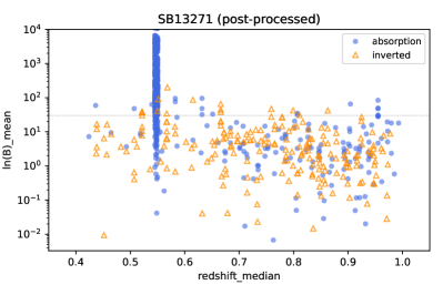
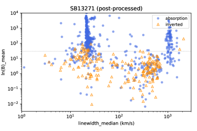
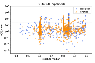
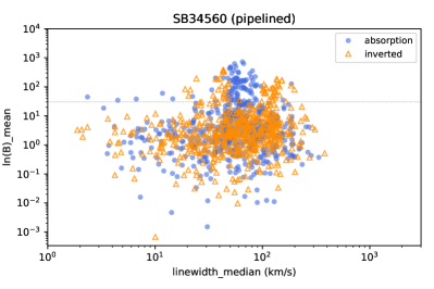
Figure 11: Plot of Bayesian evidence with ln (B) versus redshift (left) and linewidth (right) for extracted spectra from FLASH field 719, with the Pilot 1 linefinder results (top) and the Pilot 2 results (bottom). In both plots the lines found from the original absorption spectra are plotted in blue and those from the inverted spectra in orange.

8.2 Line identification in the Pilot Survey spectra

The FLASHfinder was initially run across the full 711.5–999.5 MHz range for each of the (several hundred) extracted spectra from each SBID. We use a single Gaussian model with nlive = 1000, which is the number of live points used for sampling allison12. The output data file produced by the line finder includes measurements of the following parameters and their 1$\sigma$ uncertainties, based on fitting a single Gaussian component to each candidate line:

• $z_{\rm HI}$, the redshift at the peak of the candidate line.

• $\tau_{\rm pk}$, the peak optical depth of the line.

• $\tau_{\rm int}$, the integrated optical depth of the line, in km s^-1.

• The FWHM linewidth with a single Gaussian fit of the line, in km s^-1.

• The Bayesian evidence value, ln (B), which reflects the extent to which the line detection is favoured over the null hypothesis in which no line is present (for a discussion of the relationship between ln (B) and the signal-to-noise ratio, see A).

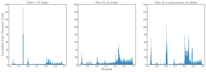
Figure 12: The false detection (artefact) count normalised by the number of fields in the absorption and inverted spectra as a function of redshift across the FLASH pilot surveys. The bin sizes correspond to the redshift range covered by 1 MHz interval. The highest peaks for the first pilot survey are mainly caused by correlator dropouts, while those from the second pilot survey are mainly due to ducted RFI.

In this initial run the linefinder was set to search at all possible redshifts in each spectrum, with no prior constraints on where a line might be. The output files for each SBID contain a set of candidate detections that may be genuine astronomical signals, spectral-line artefacts, or noise peaks.

8.3 Identifying genuine absorption lines

To distinguish astronomical signals from noise peaks, we took a conservative approach by considering only lines for which ln (B)$\geq 30$. We chose this value by inverting the original spectra and re-running the line finder on the inverted spectra (which we expect to contain only spectral artefacts and noise, since the H i emission line is too weak to be seen in the FLASH redshift range). As can be seen from Figure 11, a value of ln (B)$\sim 30$ represents an upper envelope to most of the linefinder points from the inverted spectrum, with the exception of several strong spectral artefacts seen as vertical lines in both plots.

We next aimed to distinguish astronomical signals from spectral artefacts like those shown in Figure 9. In general, we expect that an H i absorption line at any given redshift should occur in only one or two spectra in an SBID, while the spectral artefacts occur in the same position in many different spectra.

To identify repeated artefacts and spectral-line glitches at specific frequencies across many SBIDs, we aggregated the total number of detections returned by the FLASHfinder algorithm using a log-likelihood cut of ln (B)$>0$. From the histograms in Fig 12, the sharp spikes with counts above $\sim$40 correspond to regions with correlator dropouts or ducting. From these plots, we compiled a list of frequencies at which the most common spectral artefacts occurred. In general, the Pilot 2 data more often contains artefacts (see Section 7.2) than the Pilot 1 data after normalising by the number of fields observed.

8.4 Properties of the detected lines

In all, we detected 30 lines with ln (B)$>30$ that we are confident are robust detections of genuine H i absorption lines. As we will show in section 8.6, it is likely that other H i lines with smaller ln (B) values are present in the Pilot survey data, but we have not attempted to identify them at this stage and this will be the subject of a future paper.

Table 5 lists these lines, along with details of the continuum sources against which they were detected. We next extracted spectra in a smaller region around each line, and plotted the optical depth against velocity in the region around the line peak, as shown in Figure 13.

We then re-ran the line finder on these extracted spectra, after first co-adding the spectra of sources with two or more observations in Table 5. The final results for these co-added spectra are listed in Table 6 and plots of the individual spectra are shown in Figure A4.

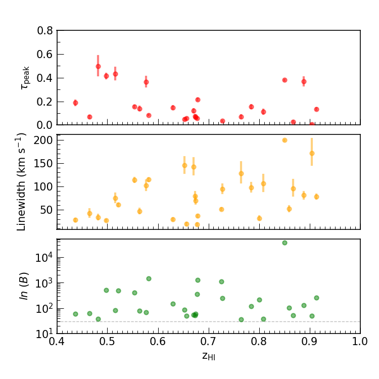
Figure 14: Peak optical depth (red) and linewidth (yellow) with 1$\sigma$ error as a function of redshift. ln (B) (green) is presented in the bottom panel with the dotted line of ln (B) = 30, the cutoff used in the linefinder search.

Fig 14 shows the optical depth, linewidth, and logarithmic Bayes number as a function of redshift. The 33 detections, including the three known detections, were found across the entire redshift range covered by the survey with linewidths ranging from $\sim$20 to 218 km s^-1.

Currently, genuine absorption lines are differentiated from spectral artefacts through visual inspection and investigation by the team. This is highly inefficient and not sustainable for the entire FLASH survey. As such, we are investigating the use of tree-based machine learning methods to improve source-identification efficiency (Liu et al. in prep.) for future FLASH observations.

(a) NVSS J015516-251423 (SB 13281 103a)

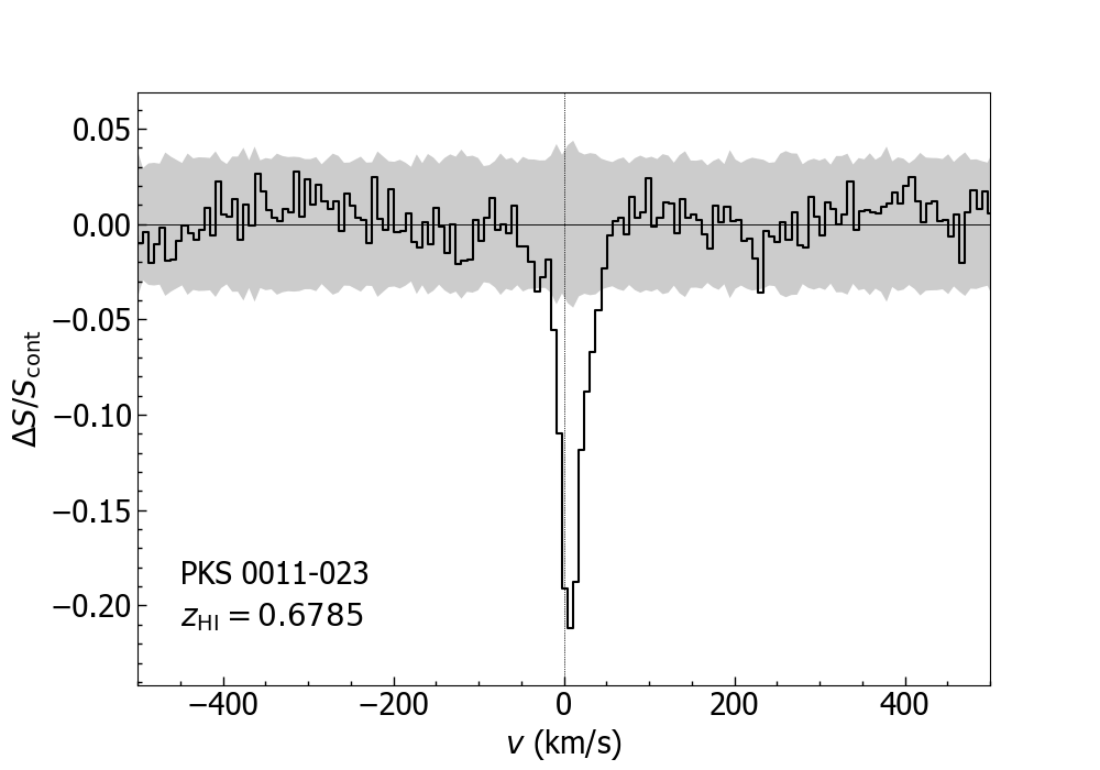
(b) PKS 0011-023 (SB 34581 9a)

Figure 13: Two strong H i absorption lines identified in Pilot Survey Phase 1 and 2. The grey band is set at five times the rms spectral-line noise. The line profiles of all the detections are added in Appendix.

8.5 Machine Learning classification of detected absorprtion lines

We expect the lines listed in Table 5 to be a mixture of intervening and associated H i absorption systems. As a preliminary way of distinguishing these in the absence of optical spectroscopy for many of our objects, we used an automated machine learning (ML) methodology curran2016b; curran2021 to classify each of the absorbers detected in this survey.

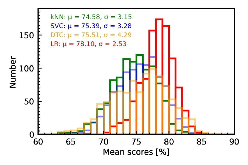
Figure 15: The distribution of the cross-validation score for 1000 trials of logistic regression (LR), k-nearest neighbour (kNN), support vector (SVC) and decision tree (DTC) classifiers.

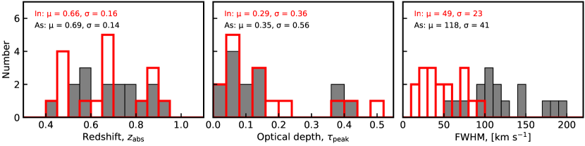
Figure 16: The distributions of the dominant model features for the putative intervening (In) and associated (As) absorbers. For the redshift and optical depth, t-tests give probabilities of p(t) = 0.64 and 0.70 of the means being the same, respectively. For the FWHM this is $p(t)=1.68\times 10^{-6}$.

We use the logistic regression (ML) classifier of curran2021, which the best performing of the other common classifiers (Figure 15) and compile the results in the final column of Table 6. To classify the lines, we used a training set of 116 out of a sample of 138 known absorbers from the literature, selected to have equal numbers of associated and intervening systems. 16 of the lines in Table 6 were classified as intervening and 14 as associated, with the line width (FWHM) being the main driver of the classification (Figure 16).

The broader associated profiles could be due to the additional nuclear component, hypothesised by unified schemes of active galactic nuclei (antonucci1993; urry1995; curran2016a, AGN, e.g.) being preferably detected through the disk of the host (curran2010, cf.), whereas intervening absorption favours face-on systems, where the coverage of the background flux is maximised curran2016b.

In the Pilot Survey sample, we find an equal mix of associated and intervening systems. A potential limitation that we note here is that the training set used consists mainly of low-z systems and contain an optical pre-selection, which may not be fully representative of the sources that could be found from an untargeted survey such as FLASH. We will return to this question in a subsequent paper discussing the host galaxies of the Pilot Survey absorption systems.

Table 5: FLASH Pilot Survey detections; (1) ID; (2) Selavy name; (3) Component ID; (4) Field name; (5) Right Ascension (deg); (6) Declination (deg); (7) frequency; (8) H i redshift; (9) optical redshift (10) closest radio source; (11) separation with the closest radio counterpart. The known detections (ID 31 to 33) were observed by previous studies; a) sadler20, b) allison15, c) chengalur1999; allison2017

ID	Selavy ID	Component	FLASH	R.A. (J2000)	DEC. (J2000)	$f_{\rm HI}$	$z_{\rm HI}$	$z_{\rm opt}$	Closest radio source	Sep.
			field	(deg)	(deg)	(MHz)				(”)
(1)	(2)	(3)	(4)	(5)	(6)	(7)	(8)	(9)	(10)	(11)
(a) Pilot 1: New detections
1	SB13290 19a	J002604-475618	123P	6.519942	-47.938337	848.3	0.6745	$-$	MRC 0023-482	1.0
2	SB13281 64a	J014141-231510	306P	25.423772	-23.253037	850.0	0.6710	$-$	NVSS J014141-231511	0.4
3	SB13281 103a	J015516-251423	306P	28.820245	-25.239974	823.4	0.7251	$-$	NVSS J015516-251423	0.4
4	SB13269 2a/2b	J025544-254741	309P	43.935136	-25.794825	857.5	0.6564	$-$	PKS 0253-259	2.0
	SB15212 9a	J025544-254739	308P	43.934931	-25.794442	857.7	0.6560			0.8
5	SB15215 27a	J045501-423858	170P	73.755747	-42.649622	859.8	0.6520	$-$	SUMSS J045501-423858	0.9
6	SB13283 228a	J090331+010847	G09B	135.881305	1.146627	933.4	0.5218	0.5226	NVSS J090331+010846	1.4
	SB11068 240a	J090331+010847	G09B_long	135.881399	1.146391	933.4	0.5218			1.4
7	SB13283 91a	J090425+012015	G09B	136.106406	1.337547	788.9	0.8004	$-$	NVSS J090425+012015	0.8
	SB11068 107a	J090425+012015	G09B_long	136.106448	1.337602	788.9	0.8004			0.8
8	SB11068 403a	J091256+030020	G09B_long	138.233859	3.005576	764.1	0.8590	$-$	NVSS J091256+030021	2.5
9	SB13271 2a	J092011+175324	719P	140.046315	17.890218	746.0	0.9040	$-$	PKS 0917+18	0.6
10	SB13271 57a	J092012+161239	719P	140.051498	16.21101	989.0	0.4362	$-$	NVSS J092012+161238	2.7
11	SB13334 64a	J113622+004850	G12A	174.091646	0.814056	908.8	0.5630	0.5629	NVSS J113622+004850	2.1
	SB13306 65a	J113622+004851	G12A_long	174.091747	0.814267	908.8	0.5630			2.1
12	SB13372 1a	J201045-242545	J2022-2507	302.688009	-24.429319	846.6	0.6778	$-$	PKS 2007-245	0.4
13	SB10849 8a	J215924-241752	351P	329.853714	-24.29795	760.4	0.8680	0.8620	MRC 2156-245	0.3
14	SB11051 35a	J223605-251918	352P	339.023937	-25.3217	948.6	0.4974	$-$	NVSS J223605-251919	2.4
15	SB11051 38a	J223619-222429	352P	339.082984	-22.408156	796.2	0.7840	$-$	NVSS J223620-222430	2.6
16	SB11051 17a	J223722-251003	352P	339.344983	-25.167529	970.2	0.4640	$-$	MRC 2234-254	1.2
17	SB15873 5a	J231351-472911	160P	348.466233	-47.486505	898.4	0.5810	$-$	PKS 2311-477	0.3
18	SB13296 158a	J233432-585646	121P	353.634345	-58.946112	900.7	0.5770	$-$	SUMSS J233432-585646	0.6
(b) Pilot 2: Repeat observations for Pilot 1 detections
(1)	SB37448 19a	J002604-475617	123	6.519433	-47.938252	848.2	0.6746	$-$	MRC 0023-482	1.0
(2)	SB37475 67a	J014141-231508	306	25.422827	-23.252426	850.2	0.6706	$-$	NVSS J014141-231511	4.2
(3)	SB37475 95a	J015516-251422	306	28.818926	-25.239542	823.4	0.7251	$-$	NVSS J015516-251423	0.4
(6)	SB34559 191a	J090331+010846	546	135.881691	1.146269	933.4	0.5218	0.5226	NVSS J090331+010846	1.4
(7)	SB34549 120a	J090425+012013	547	136.107156	1.337083	788.9	0.8004	$-$	NVSS J090425+012015	0.8
	SB34559 117a	J090425+012013	546	136.106701	1.337055	788.9	0.8004	$-$		0.8
(9)	SB34560 3a	J092011+175324	719	140.046891	17.889621	$-$	$-$	$-$	PKS 0917+18	0.6
	SB41066 3a	J092011+175324	719	140.046507	17.89018	745.9	0.9044	$-$		0.6
	SB41084 3a	J092011+175324	719	140.046165	17.8902	$-$	$-$	$-$		0.6
(10)	SB34560 55a	J092012+161236	719	140.052614	16.210097	989.0	0.4362	$-$	NVSS J092012+161238	2.7
	SB41066 56a	J092012+161238	719	140.052235	16.210709	989.0	0.4362	$-$	…	2.7
	SB41084 55a	J092012+161238	719	140.052024	16.210574	$-$	$-$	$-$	…	2.7
(11)	SB34572 65a	J113622+004850	553	174.091546	0.814248	908.8	0.5630	0.5627	NVSS J113622+004850	2.1
(17)	SB34939 5a	J231351-472911	160	348.4658	-47.486392	898.4	0.5811	$-$	PKS 2311-477	0.3
(c) Pilot 2: New detections
19	SB34581 9a	J001425-020556	525	3.606475	-2.09911	846.2	0.6785	$-$	PKS 0011-023	1.2
20	SB34581 149a	J002331+010114	525	5.881687	1.020562	937.0	0.5159	0.5160	NVSS J002331+010114	3.2
21	SB37453 1a	J040757-275705	311	61.991078	-27.951503	822.0	0.7280	0.7280	PKS 0405-280	1.7
22	SB34570 50a	J051805-245502	314	79.524788	-24.917494	914.1	0.5538	$-$	NVSS J051806-245502	1.7
	SB41061 50a	J051805-245502	314	79.525186	-24.917212	914.1	0.5538	$-$		1.7
	SB41065 51a	J051805-245502	314	79.525202	-24.917451	914.1	0.5538	$-$		1.7
23	SB41061 1a	J053354-234430	314	83.477481	-23.741721	767.5	0.8507	0.8510	MRC 0531-237	0.8
	SB41065 1a	J053354-234430	314	83.477565	-23.74192	767.5	0.8508	0.8510		0.8
24	SB34571 8a	J094650-202045	377	146.709164	-20.345918	742.3	0.9134	0.9130	NVSS J094650-202044	0.9
25	SB34561 188a	J100238-195919	378	150.660845	-19.988637	958.7	0.4815	$-$	NVSS J100238-195917	2.0
26	SB34576 62a	J150506+022928	561	226.278737	2.491188	785.4	0.8085	0.8050	NVSS J150506+022927	0.5
27	SB34552 19a	J170135-294917	287	255.398288	-29.821407	871.4	0.6299	$-$	NVSS J170135-294918	1.8
28	SB34566 100a	J205147+021738	575	312.949592	2.294018	752.2	0.8883	$-$	NVSS J205147+021740	2.1
	SB34577 94a	J205147+021740	575	312.949333	2.294467	752.2	0.8884	$-$		2.1
29	SB34597 47a	J223317-015739	579	338.321991	-1.960909	848.8	0.6734	$-$	NVSS J223317-015739	0.3
	SB42298 45a	J223317-015739	579	338.322054	-1.961156	848.9	0.6733	$-$		0.3
30	SB34556 46a	J233703-015210	582	354.262692	-1.869491	805.0	0.7645	$-$	NVSS J233702-015209	1.7
(d) Pilot 2: Observations of known strong absorption lines
31	SB34564 2a	J161749-771717	011	244.455916	-77.28819	979.4	0.4502	1.7100	PKS 1610-77a)	1.1
32	SB34553 1a	J174425-514442	151	266.10647	-51.745095	988.1	0.4413 (A15)	0.4413	PKS 1740-517b)	1.7
33	SB33616 1a	J183339-210339	398	278.416187	-21.061056	753.5	0.8851	0.8850	PKS 1830-21c)	0.1

Table 6: FLASHfinder results for co-added spectra; (1) ID; (2) Source name; (3) N; (4) Field name; (5) Continuum flux density; (6) H i redshift; (7) Peak optical depth and uncertainty; (8) Integrated optical depth and uncertainty; (9) Linewidth and uncertainty; (10) ln (B); (11) Notes (N = Individual Note in Appendix B); (18) Machine Learning (ML) classification, using the methodology of Curran (2021), where ‘As’ indicates a probable associated line and ‘In’ a probable intervening line, see Section 8.5. The uncertainties in colum (7) to (9) represent the 68% credible interval about the median.

ID	Source name	Nspec	FLASH	Scont.	$z_{\rm HI}$	$\tau_{\rm peak}$	$\tau_{\rm int}$	Linewidth	ln (B)	Notes	ML
			field	(Jy)				(km s-1)			class
(1)	(2)	(3)	(4)	(5)	(6)	(7)	(8)	(9)	(10)	(11)	(12)
1	MRC 0023-482	2	123	0.379	0.6745	$0.066\begin{subarray}{c}+0.007\\ -0.007\end{subarray}$	$4.63\begin{subarray}{c}+0.47\\ -0.46\end{subarray}$	$70.0\begin{subarray}{c}+7.8\\ -7.1\end{subarray}$	58.7	N	In
2	NVSS J014141-231511	2	306	0.137	0.6707	$0.122\begin{subarray}{c}+0.014\\ -0.014\end{subarray}$	$17.42\begin{subarray}{c}+1.91\\ -1.92\end{subarray}$	$142.2\begin{subarray}{c}+18.7\\ -16.1\end{subarray}$	55.2		As
3	NVSS J015516-251423	2	306	0.103	0.7251	$1.830\begin{subarray}{c}+0.119\\ -0.105\end{subarray}$	$94.53\begin{subarray}{c}+4.31\\ -4.08\end{subarray}$	$51.6\begin{subarray}{c}+1.7\\ -1.6\end{subarray}$	1121.3		As
4	PKS 0253-259	2	308/309	0.705	0.6564	$0.057\begin{subarray}{c}+0.006\\ -0.006\end{subarray}$	$1.12\begin{subarray}{c}+0.13\\ -0.12\end{subarray}$	$19.7\begin{subarray}{c}+2.6\\ -2.3\end{subarray}$	50.4		In
5	SUMSS J045501-423858	1	170	0.288	0.6525	$0.051\begin{subarray}{c}+0.005\\ -0.005\end{subarray}$	$7.38\begin{subarray}{c}+0.70\\ -0.67\end{subarray}$	$145.7\begin{subarray}{c}+17.5\\ -16.4\end{subarray}$	86.2		As
6	NVSS J090331+010846	2	G09B/546	0.059	0.5218	$1.748\begin{subarray}{c}+0.155\\ -0.145\end{subarray}$	$106.74\begin{subarray}{c}+6.93\\ -6.68\end{subarray}$	$61.1\begin{subarray}{c}+2.4\\ -2.4\end{subarray}$	483.8		As
7	NVSS J090425+012015	3	G09B/546/547	0.087	0.8004	$1.158\begin{subarray}{c}+0.146\\ -0.127\end{subarray}$	$37.42\begin{subarray}{c}+2.79\\ -2.74\end{subarray}$	$32.1\begin{subarray}{c}+3.5\\ -3.0\end{subarray}$	210.7		In
8	NVSS J091256+030021	1	G09B_long	0.033	0.8592	$1.255\begin{subarray}{c}+0.212\\ -0.176\end{subarray}$	$64.93\begin{subarray}{c}+7.09\\ -6.64\end{subarray}$	$51.7\begin{subarray}{c}+5.7\\ -5.4\end{subarray}$	104.7		In
9	PKS 0917+18	2	719	1.791	0.9044	$0.008\begin{subarray}{c}+0.001\\ -0.001\end{subarray}$	$1.37\begin{subarray}{c}+0.17\\ -0.16\end{subarray}$	$171.5\begin{subarray}{c}+30.4\\ -25.4\end{subarray}$	48.7		As
10	NVSS J092012+161238	3	719	0.171	0.4362	$0.188\begin{subarray}{c}+0.021\\ -0.019\end{subarray}$	$5.28\begin{subarray}{c}+0.55\\ -0.53\end{subarray}$	$28.0\begin{subarray}{c}+3.0\\ -2.6\end{subarray}$	58.3		In
11	NVSS J113622+004850	3	G12A/553	0.154	0.5632	$0.140\begin{subarray}{c}+0.014\\ -0.014\end{subarray}$	$6.57\begin{subarray}{c}+0.61\\ -0.61\end{subarray}$	$46.9\begin{subarray}{c}+5.3\\ -4.5\end{subarray}$	76.8		In
12	PKS 2007-245	1	J2022-2507	1.827	0.6778	$0.056\begin{subarray}{c}+0.003\\ -0.003\end{subarray}$	$1.06\begin{subarray}{c}+0.07\\ -0.06\end{subarray}$	$19.0\begin{subarray}{c}+1.8\\ -1.7\end{subarray}$	358.5		In
13	NVSS J215924-241752	1	351	0.806	0.8679	$0.028\begin{subarray}{c}+0.004\\ -0.004\end{subarray}$	$2.69\begin{subarray}{c}+0.35\\ -0.32\end{subarray}$	$95.0\begin{subarray}{c}+19.1\\ -14.9\end{subarray}$	52.7		In
14	NVSS J223605-251919	1	352	0.215	0.4974	$0.414\begin{subarray}{c}+0.021\\ -0.019\end{subarray}$	$11.29\begin{subarray}{c}+0.45\\ -0.47\end{subarray}$	$27.2\begin{subarray}{c}+1.3\\ -1.3\end{subarray}$	515.0		In
15	NVSS J223620-222430	1	352	0.207	0.7846	$0.157\begin{subarray}{c}+0.013\\ -0.012\end{subarray}$	$15.32\begin{subarray}{c}+1.26\\ -1.18\end{subarray}$	$97.7\begin{subarray}{c}+9.6\\ -8.3\end{subarray}$	115.9		As
16	MRC 2234-254	1	352	0.343	0.4641	$0.071\begin{subarray}{c}+0.010\\ -0.009\end{subarray}$	$3.06\begin{subarray}{c}+0.39\\ -0.35\end{subarray}$	$42.9\begin{subarray}{c}+8.1\\ -7.6\end{subarray}$	60.9		In
17	PKS 2311-477	2	160	0.998	0.5811	$0.084\begin{subarray}{c}+0.002\\ -0.002\end{subarray}$	$9.65\begin{subarray}{c}+0.22\\ -0.21\end{subarray}$	$114.6\begin{subarray}{c}+2.8\\ -2.7\end{subarray}$	1428.4		As
18	SUMSS J233432-585646	1	121	0.074	0.5769	$0.365\begin{subarray}{c}+0.042\\ -0.040\end{subarray}$	$37.38\begin{subarray}{c}+3.60\\ -3.77\end{subarray}$	$102.1\begin{subarray}{c}+11.1\\ -10.0\end{subarray}$	68.6		As
19	PKS 0011-023	1	525	0.694	0.6785	$0.216\begin{subarray}{c}+0.007\\ -0.006\end{subarray}$	$7.90\begin{subarray}{c}+0.20\\ -0.20\end{subarray}$	$36.6\begin{subarray}{c}+1.2\\ -1.2\end{subarray}$	1239.9	N	In
20	NVSS J002331+010114	1	525	0.067	0.5159	$0.431\begin{subarray}{c}+0.052\\ -0.047\end{subarray}$	$32.30\begin{subarray}{c}+3.20\\ -3.06\end{subarray}$	$74.8\begin{subarray}{c}+9.6\\ -8.4\end{subarray}$	80.4		As
21	PKS 0405-280	1	311	1.278	0.7280	$0.035\begin{subarray}{c}+0.002\\ -0.002\end{subarray}$	$3.34\begin{subarray}{c}+0.22\\ -0.22\end{subarray}$	$94.6\begin{subarray}{c}+9.4\\ -9.1\end{subarray}$	242.4		As
22	NVSS J051806-245502	3	314	0.186	0.5538	$0.156\begin{subarray}{c}+0.007\\ -0.006\end{subarray}$	$17.85\begin{subarray}{c}+0.68\\ -0.70\end{subarray}$	$114.2\begin{subarray}{c}+3.9\\ -4.1\end{subarray}$	411.4		As
23	MRC 0531-237	2	314	1.746	0.8508	$0.381\begin{subarray}{c}+0.002\\ -0.002\end{subarray}$	$75.82\begin{subarray}{c}+0.35\\ -0.35\end{subarray}$	$199.1\begin{subarray}{c}+0.8\\ -0.7\end{subarray}$	36724.9		As
24	NVSS J094650-202044	1	377	0.550	0.9134	$0.135\begin{subarray}{c}+0.007\\ -0.007\end{subarray}$	$10.61\begin{subarray}{c}+0.54\\ -0.54\end{subarray}$	$78.2\begin{subarray}{c}+4.2\\ -4.0\end{subarray}$	252.4		In
25	NVSS J100238-195917	1	378	0.057	0.4815	$0.499\begin{subarray}{c}+0.082\\ -0.077\end{subarray}$	$17.16\begin{subarray}{c}+2.31\\ -2.24\end{subarray}$	$34.2\begin{subarray}{c}+5.4\\ -4.3\end{subarray}$	38.3		In
26	NVSS J150506+022927	1	561	0.150	0.8085	$0.112\begin{subarray}{c}+0.017\\ -0.015\end{subarray}$	$11.93\begin{subarray}{c}+1.54\\ -1.50\end{subarray}$	$106.4\begin{subarray}{c}+18.8\\ -16.0\end{subarray}$	37.7		As
27	NVSS J170135-294918	1	287	0.403	0.6299	$0.149\begin{subarray}{c}+0.011\\ -0.011\end{subarray}$	$4.43\begin{subarray}{c}+0.30\\ -0.30\end{subarray}$	$29.8\begin{subarray}{c}+2.1\\ -2.1\end{subarray}$	146.5		In
28	NVSS J205147+021740	2	575	0.111	0.8884	$0.368\begin{subarray}{c}+0.035\\ -0.032\end{subarray}$	$29.91\begin{subarray}{c}+2.35\\ -2.35\end{subarray}$	$81.0\begin{subarray}{c}+7.3\\ -6.9\end{subarray}$	127.3		In
29	NVSS J223317-015739	2	579	0.235	0.6734	$0.074\begin{subarray}{c}+0.008\\ -0.008\end{subarray}$	$5.91\begin{subarray}{c}+0.62\\ -0.63\end{subarray}$	$79.0\begin{subarray}{c}+9.4\\ -7.8\end{subarray}$	51.9		In
30	NVSS J233702-015209	1	582	0.232	0.7645	$0.072\begin{subarray}{c}+0.010\\ -0.010\end{subarray}$	$9.26\begin{subarray}{c}+1.23\\ -1.21\end{subarray}$	$127.8\begin{subarray}{c}+23.5\\ -19.2\end{subarray}$	36.6		As

8.6 Completeness tests

Next, we investigated the completeness of the FLASHfinder H i 21-cm detections using the techniques described by allison20 and allison22. The completeness is defined as the probability of recovering an absorption feature with a given peak signal-to-noise ratio (S/N; in an 18.5 kHz channel) and line width (in $\rm km~{}s^{-1}$) from the spectrum, using the linefinder allison12.

This is estimated by selecting 100 spectra randomly from a sample of ‘test’ spectra, and inducing a Gaussian absorption line with a specific peak signal-to-noise ratio (S/N) and line width in each spectrum at random locations. Then the linefinder is run on these 100 spectra, after which we estimate the fraction of the recovered absorption lines. We made two separate run. The first run used a detection limit of ln (B) $>20$, which is slightly deeper than the threshold described in the earlier sections, to test the depth of our threshold. The second run used a detection limit of ln (B) $>30$, consistent with our usual threshold.

We repeat this process over a wide range of combinations of S/N and line width. The completeness, i.e. the fraction of recovered lines, is plotted as a bivariate function for each peak S/N - line width combination (see e.g. Figure 17). The function is finally smoothed using a Savitzky-Golay filter savitzky1964.

For these tests, we used spectra from two SBIDs, SB 34917 and SB 34581. The spectra of SB 34917 are known to be clean, without any significant RFI/ducting features or wobbles in the spectra. The completeness fractions with a detection limit of ln (B) $=20$ show a relatively smaller scatter compared to those with ln (B)$=30$. Also, the curves are slightly shifted towards lower peak S/N values in the plot with ln (B) $=20$, implying that a larger fraction of weaker lines are detected.

In Figure 18 we plot the completeness fractions for SB 34581, using a detection limit of ln (B) $=20$. The spectra in these observations are corrupted by wobbles and ducting. The effects of these can be seen in the completeness plots; the detection fractions are not optimum for various FWHM and peak S/N combinations.

We see from Figure 17 that the completeness functions of SB 34917 are smooth, and reach $100\%$ detection fractions quickly for peak S/Ns $>10$ and line widths $\rm>10\ km\ s^{-1}$. However, for SB 34581 in Figure 18, the functions are not smooth, and the fractions do not reach $100\%$ for most combinations of peak S/N and and line width. This is because of the reduced efficacy of the automated line finder in identifying the induced Gaussian absorption feature, among spectral wobbles and RFI/ducting features.

In our tests using the clean spectra (Figure 17, the right panel), we achieve 80 to 100% completeness in recovering broader lines with widths exceeding 80 km s^-1 (red and orange lines), for a given peak S/N of 3. This corresponds to the significance of ln(B) $=30$ as detailed in Appendix A.1. Meanwhile, in order to reach a certain completeness level, narrower lines requires higher peak S/N values.For instance, to achieve 50% completeness overall, peak S/N values of approximately 4, 6, 8, and 12 are needed for line widths of 40, 20, 10, and 5 km s^-1, respectively (light green to purple lines). It is important to note that the observation’s channel resolution ranges from 8 to 19 km s^-1.

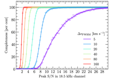
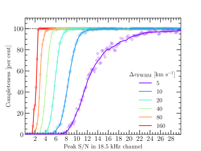
Figure 17: The completeness fractions plotted as a function of the peak signal-to-noise ratio for data from a good-quality observation (SB 34917). The colours represent a set of lines of different FWHMs, as indicated in the legend. The linefinder detection limit is set at ${\rm ln\,(B)}~{}>20$ for the left-hand plot, and at ${\rm ln\,(B)}~{}>30$ for the right-hand plot. Further details are provided in Section 8.6.

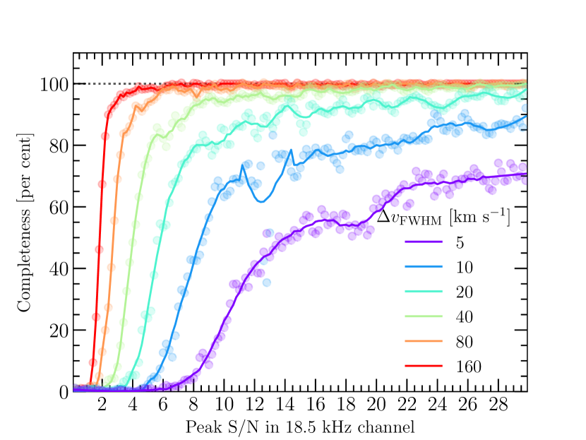
Figure 18: Similar to the left-hand plot of Figure 17, but for an observation (SB 34681) where the data suffered from the spectral ‘wobbles’ discussed in Section 7.2.

8.7 Comparison of repeat observations

Up to one-third of the FLASH Pilot Survey fields were observed more than once. These repeat observations occurred for several different reasons:

1. Repeat observations in Pilot 2 of five Pilot 1 fields with a total of seven detected H i absorption lines. These repeats were intended to test the reproducibility of the ASKAP detections and line profiles.

2. Repeat observations of the GAMA 09h, 12h and 15h fields. The deeper (6 hr) observations carried out in Pilot 1 allow us to check for weak lines close to the noise threshold for the standard (2 hr) FLASH fields. The reobservation of these fields in Pilot 2, on slightly different field centres, provides additional tests of reproducibility.

3. Repeat observations of Pilot 2 fields. These repeats were made either because of artefacts in the original data, or to test the effects of changes in observing configuration. These observations potentially provide some insights into the detectability of lines in non-ideal data.

From the data in Table 5, we identified fifteen pairs of observations of the same lines for which linefinder measurements could be compared. Figure 19 shows the values of redshift $z$, peak optical depth $\tau_{\rm pk}$, integrated optical depth $\tau_{\rm int}$ and velocity width $\Delta{\rm V}$ measured for these pairs of lines. For each pair of lines, we also calculated the peak difference between pairs of observations for each of the four parameters.

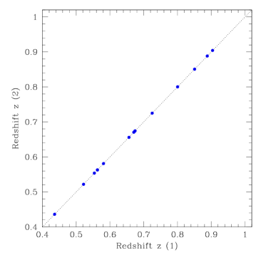
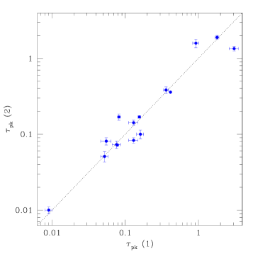
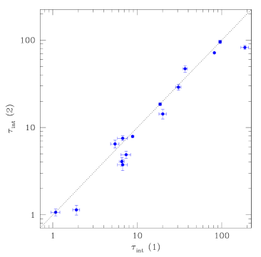
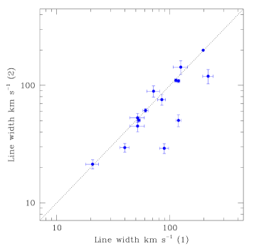
Figure 19: Comparison of linefinder results for repeat observations. All values are for a single gaussian fit to the line profile, and the error bars show the uncertainties given by the linefinder.

From this comparison, we find that measurements of redshift are highly reproducible (differing by $<<0.1$%) while measurements of peak and integrated optical depth have typical uncertainties of around 25%. Measurements of line width (fitting a single component) have a typical uncertainty of around 20%. We also conclude that the quoted uncertainties (68% credible interval about the median) listed in the FLASHfinder output are generally an accurate reflection of the true observational uncertainties, with a small number of outliers.

8.8 Radio continuum properties of H i detected sources

All the continuum sources where we deteted an H i line were unresolved in the highest-resolution (12-15 arcsec beam) FLASH continuum images. To obtain more information about these compact sources, we performed broadband spectral modelling using flux density measurements from the literature.

Modelling of the Spectral Energy Distributions (SEDs) of Pilot Survey detections was performed with RadioSED, a Bayesian inference package designed for use with broadband radio continuum data kerrison2024. Radio flux densities were compiled from a number of large-area, publicly available continuum surveys to construct individual SEDs (see Table 1 of kerrison2024 for more details). RadioSED then inferred the most likely of four analytical models for each SED using nested sampling for Bayesian evidence estimation. The models used can capture various degrees of spectral curvature, including the ability to identify peaked spectrum sources ODea2021, but assume minimal broadband variability.

In the case of three detections, NVSS J002331+010114, NVSS J090425+012015, and NVSS J090331+010846, additional LOFAR data were acquired via private communication to better constrain the source SEDs in the megahertz regime. These data are drawn from the forthcoming LoTSS survey shimwell2022.

The radio SEDs of the sources with H i detections are plotted in Figure A4 alongside the H i spectra.

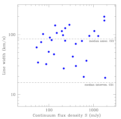
Figure 20: Properties of the H i lines detected against continuum sources of different flux densities. (left) The peak optical depth $\tau_{\rm pk}$, with a dashed line showing the expected sensitivity of the FLASH survey as calculated by allison12 and a vertical dotted line showing the 45 mJy limit adopted for the H i line search. (right) The line width in km s^-1, as listed in Table 6. In both plots, horizontal dashed lines show the median values for the associated and intervening absorption lines in the literature compilation of curran2021.

9 Discussion

9.1 General remarks on data quality

The quality of the spectral-line data obtainable from the radio-quiet ASKAP site can be extremely good, as can be seen from the example spectrum shown in Figure 6, with the FLASH band from 712–1000 MHz generally free from terrestrial RFI.

Overall though, the quality of the pilot survey data was variable and most of the processed data released in CASDA are classified as being of ‘uncertain’ quality. This is perhaps to be expected from early observations with a new telescope coupled with a sophisticated data processing pipeline. As discussed earlier, data from the first pilot survey suffered from correlator dropouts and needed post-processing because of an incorrect implementation of the beam-forming intervals, while the data from the second pilot survey was affected by several spectral-line artefacts. Most of these problems have now been overcome, and should not affect future FLASH observations.

9.2 Properties of the detected H i  lines

The H i lines detected in the pilot survey span a wide redshift range from $z=0.43$ to $z=0.91$, and have velocity widths between 19 and 199 km s^-1. Figure 20 shows the distribution of optical depth and line width for the detected lines.

The left-hand plot in Figure 20 shows that the limiting peak optical depth that can be detected increases at lower flux densities, as expected for an absorption-line search. The lower bound for the detected lines lies close to the diagonal line in this plot, which shows the expected FLASH sensitivity limit calculated by allison12. In other words, we are reaching the optical-depth sensitivity expected when the FLASH survey was first proposed more than a decade ago.

A second point to note from this plot is the high peak optical depth of most of our detected lines. Our sample contains three lines with a peak optical depth $\tau_{\rm pk}>1.0$, larger than any of the 136 lines in the curran2021 compilation of literature data. The median value of $\tau_{\rm pk}=0.148$ for our detected lines is significantly higher than the median $\tau_{\rm pk}=0.030$ for the literature sample compiled by curran2021. This is consistent with the prediction by allison22 that FLASH would detect a population of lines with very high optical depth.

9.3 H i  detection rate in the pilot surveys

We now compare the overall detection rate of H i lines in the FLASH pilot surveys with the rate predicted by allison22.

In Table 3 of their paper, allison22 estimate the total number of H i detections expected from a FLASH survey covering 903 ASKAP fields. For an assumed H i spin temperature T${}_{\rm S}=300$ K, the estimated rate is around 3.1 lines per ASKAP field (with 70% of these being associated lines and 30% intervening lines). However, allison22 also caution that these estimates are highly uncertain, particularly for the population of associated lines.

The H i detection rate in the FLASH Pilot Surveys is significantly lower than the allison22 estimate. In the first pilot survey we detected 17 new lines from 37 fields, a rate of 0.46 lines per field. In the second pilot survey the rate was even lower, with 12 detections from the 38 fields not previously observed - a rate of 0.32 lines per field. The lower detection rate for the second pilot survey is probably due to the large number of sources with spectral wobbles that reduce the completeness of the linefinder search (see Figure 18). For this reason, we adopt the Pilot 1 value of 0.5 lines per field as an indicative H i detection rate for the pilot surveys.

Turning to the allison22 estimates, we make two adjustments based on recent results.

1. For associated H i absorption lines, allison22 assume a detection rate of 10%, but also note that “…the actual detection rate could be even less than assumed here, and hence our predictions are purely indicative of the results that may be obtained from a large unbiased radio-selected survey.”

   Recently, the actual detection rate for associated H i absorption at $0.4<z<1$ has been measured by su2022 and aditya2024 using FLASH pilot survey data. Both studies used samples for which optical spectroscopy was available, and used the optical redshift as a prior to the linefinder H i search. su2022 searched a sample of radio-detected galaxies in the GAMA 9, 12, and 15 fields and found a detection rate of 2.9% for associated lines with $\tau_{\rm pk}>0.1$, while aditya2024 found a detection rate of 1.8% for a sample of 62 bright radio galaxies from the MRC-1Jy sample mccarthy1996.

   These measurements are consistent with other work suggesting a lower detection rate for associated H i absorption at higher redshifts curran2019; aditya18, either because the gas spin temperature is higher or the gas is largely ionized by a powerful central AGN.

2. curran2021 show that intervening H i absorption lines are typically much narrower than associated lines, but the completeness tests in Section 8.6 of this paper show that, for a given peak SNR, narrow lines are harder to detect than broad lines, especially for fainter sources. The data in Figure 20 also confirm this. The narrowest line we detected in the pilot survey has a width of 19 km s^-1, but over half of the intervening lines listed by curran2021 have line widths below 20 km s^-1, suggesting that our current sample is likely to be incomplete for narrow intervening lines. An additional limitation of the pilot survey is that narrow H i lines could be confused with narrow spectral artefacts such as glitches.

If we assume a lower detection rate of 3% rather than 10% for associated H i lines, and also assume that around 50% of intervening lines were missed in the Pilot Survey data because they were narrower than 20 km s^-1, then the detection rate estimated by allison22 drops from 3.1 overall to 1.1 line per field for lines with velocity width above 20 km s^-1 (with roughly 60% of these being associated lines and 40% intervening).

A detection rate of 1.1 lines per field is still a factor of two higher than we observed in the FLASH pilot surveys. This could mean that the gas spin temperature is typically higher than the 300 K assumed by allison22, yielding a lower observed optical depth. However, we also imposed a cut of ln (B)$>30$ on the linefinder results whereas the completeness tests in Section 8.6 imply that many lines with ln (B)$<30$ are reliably identified by the linefinder. This leaves open the possibility that we could set a lower ln (B) limit for the full FLASH survey if the data are largely free of spectral artefacts.

9.4 Verification of FLASH data using MeerKAT

A subset of the H i absorption lines detected in the FLASH pilot surveys were observed with MeerKAT to better characterise the absorption lines with higher S/N. These observations were carried out under the program ID SCI-20210212-EM-01 and used the UHF band covering the frequency range of $580-1015$ MHz with the 32K mode correlator giving a similar spectral resolution of 16.6 kHz compared to ASKAP’s 18.5 kHz. Each target was observed for a total integration time of 1 hr. A complete analysis of the MeerKAT observations will be the subject of future papers (Mahony et al. in prep., and Glowacki et al. in prep.), but we present initial results here for data verification purposes.

Figure 21 shows the ASKAP-FLASH and MeerKAT spectra of two Pilot Survey detections (J090425+012015 at $z_{\rm HI}=0.80$ and J092012+161238 at $z_{\rm HI}=0.44$). With the exception of the higher S/N provided by the MeerKAT observations, the ASKAP and MeerKAT spectra match remarkably well and nicely demonstrate the spectral line capabilities and fidelity afforded by these two SKA precursor telescopes on radio-quiet sites.

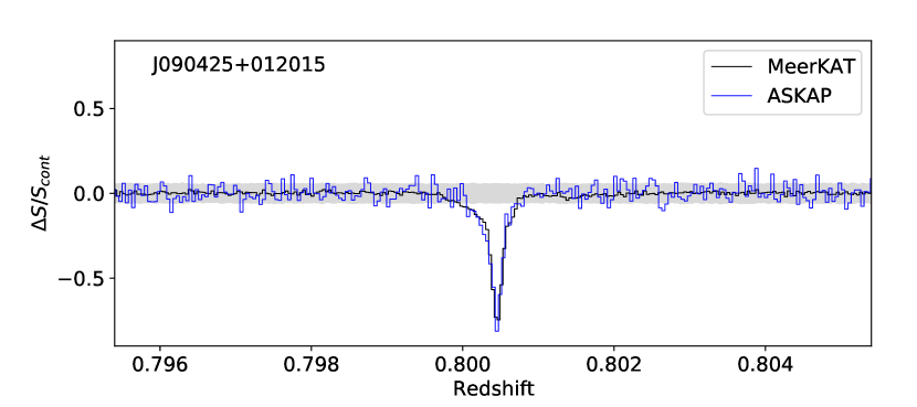
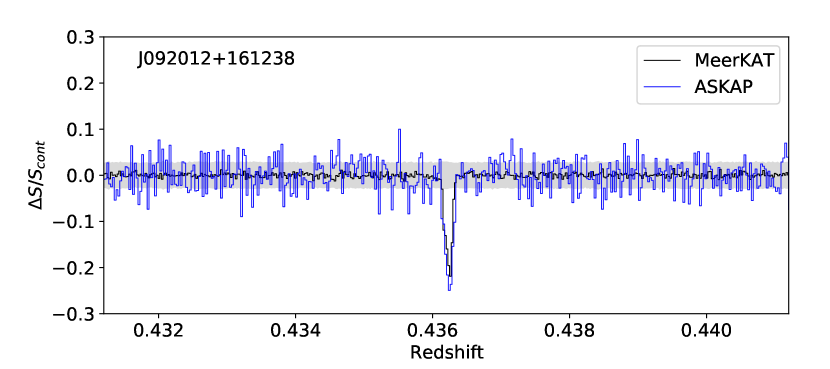
Figure 21: Spectra of FLASH detections observed with MeerKAT (black line) overlaid with the ASKAP spectrum (blue). The grey band denotes the 5-$\sigma$ noise level calculated from the MeerKAT spectra.

9.5 Future work

Following the two phases of Pilot observations, we began the full five-year FLASH survey in late 2022. The full FLASH survey will cover 600 fields ASKAP fields (a total of 24,000 deg²) rather than the 903 fields originally planned, with the allocated 1200 hours of observing time. The coverage will span declinations from $-90$ to $+18$ degrees at Galactic latitudes $|b|\geq 8.5$ deg. Our pilot survey results suggest that the full FLASH survey will detect between 300 and 600 new absorption lines, with around 60% of these being associated lines.

The next paper in this series will identify the host galaxies of the H i lines discovered in the pilot surveys, and will also discuss how best to determine whether an individual line is associated or intervening.

10 Summary

The FLASH pilot surveys are pioneering studies that search for H i absorption lines in and around distant galaxies without any optical preselection of targets. We have identified a sample of 30 new robustly-detected absorption lines, several of which have higher optical depths than any previously-known line. This work has led us to make new predictions about the detection rate for the full FLASH survey, highlighting its potential impact on our understanding of H i absorption systems.

We successfully tested and demonstrated the automatic data pipeline for the survey and made public immediately after validation, with no proprietary period. We also used a powerful Bayesian line finder to identify and parameterise absorption lines in a consistent and uniform way. Observations of a subset of these lines with the MeerKAT telescope show a high degree of consistency, implying that both telescopes produce high-quality, reproducible spectral-line data.

The three main aims of the FLASH Pilot Surveys have all been achieved.

Firstly, we were able to test and demonstrate an end-to-end data pipeline for the FLASH survey and make line detections that are robust, reproducible, and have a statistical significance attached. We also identified several improvements that could be made in future, including masking out spectral-line artefacts before running the line finder, fitting multiple components to the absorption lines, and further investigating the completeness and detectability of faint and narrow spectral lines.

Our second goal was to determine the H i detection rate for associated absorption lines at $0.4<z<1$. This was done in two companion papers that were able to use optical redshifts as a prior for the line search su2022; aditya2024. In the redshift range covered by FLASH, the detection rate for associated H i lines is 2–3% for the source population as a whole, rising to around 23% for compact radio sources less than about 1 arcsec in size.

Finally, we have made new predictions of the detection rate for the full FLASH survey, showing that FLASH is likely to detect 300–600 new H i absorption systems at $0.4<z<1.0$. This represents an order of magnitude more detections than currently available in this redshift range, and should enable us to constrain the average spin temperature and/or H i mass density at intermediate redshifts.

This scientific work uses data obtained from Inyarrimanha Ilgari Bundara / the Murchison Radio-astronomy Observatory. We acknowledge the Wajarri Yamaji People as the Traditional Owners and native title holders of the Observatory site. CSIRO’s ASKAP radio telescope is part of the Australia Telescope National Facility (https://ror.org/05qajvd42). Operation of ASKAP is funded by the Australian Government with support from the National Collaborative Research Infrastructure Strategy. ASKAP uses the resources of the Pawsey Supercomputing Research Centre. Establishment of ASKAP, Inyarrimanha Ilgari Bundara, the CSIRO Murchison Radio-astronomy Observatory and the Pawsey Supercomputing Research Centre are initiatives of the Australian Government, with support from the Government of Western Australia and the Science and Industry Endowment Fund.

This research was supported by the Australian Research Council Centre of Excellence for All Sky Astrophysics in 3 Dimensions (ASTRO 3D) through project no. CE170100013.

This work was supported by the LAMP Program of the National Research Foundation of Korea (NRF) grant funded by the Ministry of Education (No. RS-2023-00301976).

ACE acknowledges support from STFC grant ST/P00541/1. KG is supported by the Australian Research Council through the Discovery Early Career Researcher Award (DECRA) Fellowship (project number DE220100766) funded by the Australian Government.

The MeerKAT telescope is operated by the South African Radio Astronomy Observatory, which is a facility of the National Research Foundation, an agency of the Department of Science and Innovation.

Appendix A A note on Bayesian ln B values and statistical significance

In this paper we have used a Bayesian evidence parameter ln (B) to identify absorption lines in ASKAP spectra. Here, we briefly discuss the relationship between ln (B) and the statistical n $\sigma$ uncertainty often used by the wider astronomy community to assess the significance of a result.

The calibration from frequentist p-values, or ‘sigma significance levels’ to the Bayes factor has been discussed in detail by sellke2001 and trotta2008. trotta2008 also provides an empirical scale for evaluating the strength of evidence when comparing two models, with ln (B) = 5 corresponding to ‘strong evidence’ (a 3.6 $\sigma$ result, with p $=0.0003$) and ln (B) = 11 to a 5$\sigma$ value. benneke2013 apply Bayesian methods to a specific problem in exoplanet atmospheres and provide an expanded version of the trotta2008 Bayes to frequentist ‘translation table’.

In the context of our FLASH absorption-line finding problem, the Bayes value is the odds ratio of obtaining the observed data (assuming the absorption-line model is correct) versus just gaussian noise. The p-value is the probability of obtaining data features that are at least as extreme as those observed assuming just Gaussian noise. In both cases no consideration is made for non-Gaussian noise or artefacts - which we know are present in the ASKAP Pilot Survey data (see Figure 9).

We therefore stress that all statistics quoted in this paper (whether B, p-values and/or sigmas) are calculated with respect to the assumed Gaussian noise and not any other non-Gaussian noise features.

To examine the empirical relationship between ln (B) and the signal-to-noise ratio (SNR) in our current set of line detections, we calculated an approximate peak SNR for each FLASH detection using the single spectrum in which the line was first detected. We then calculated the size of the ‘dip’ in the continuum at the line peak from the continuum flux density and the observed peak optical depth $\tau_{\rm pk}$ and divided this by an assumed noise of 5.5 mJy per beam in a single channel.

The results are shown in Figure A1, where dotted lines show a peak SNR of 3 $\sigma$ and our adopted cutoff for detections of ln B = 30. We need to keep in mind that the SNR in this plot is a peak value, while ln (B) is calculated for the whole line rather than a single channel. Nevertheless, there is a reasonable correlation that suggests we are detecting lines with peak SNR greater than about 2.5 to 3 $\sigma$.

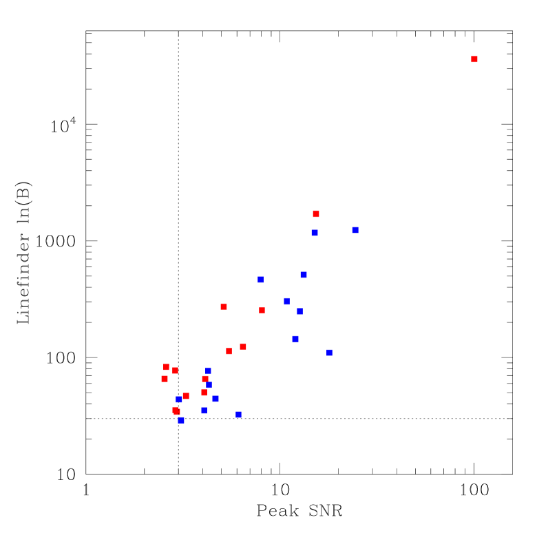
Figure A1: Relationship between the linefinder ln (B) value and estimated peak SNR for the H i absorption lines detected in the Pilot Survey. Blue points represent lines with velocity width $<80$ km s^-1, and red points show broader lines with velocity width $\geq 80$ km s^-1. The horizontal line at ln (B) = 30 shows the cutoff value used in this paper to select line detections and the vertical dotted line corresponds to a 3$\sigma$ detection of the line peak.

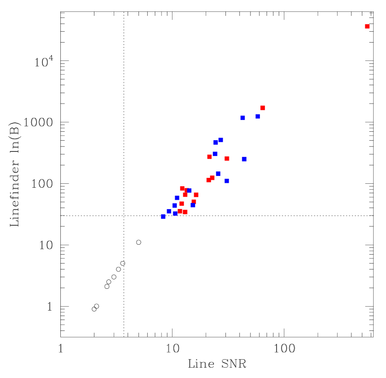
Figure A2: As in Figure A1, except that the SNR values plotted are now integrated over the whole line, assuming a gaussian profile. In this plot, black open circles at lower ln B show values tabulated by benneke2013 and the vertical dotted line corresponds to the 3.6 $\sigma$ value considered by trotta2008 to be ‘strong’ evidence.

Figure A2 shows SNR values integrated over the whole line, which takes into account the range of line wdiths present in our data. Values from Table 2 of benneke2013 are plotted as open circles, and our data extend the benneke2013 values out to much higher values of ln (B). This plot implies that an absorption line with ln (B)$\geq 30$ has a line SNR $\geq 7-8$ and is therefore a highly significant detection. It also implies that (in the absence of artefacts) we should be able to detect lines down to values of ln (B) $\sim 10$. Such detections may become possible in future if we can apply machine learning algorithms to distinguish artefacts from astronomical signals in a reliable way.

Appendix B Notes on individual objects

PKS 0011-023 (J001425-020556): dunlop1989 list an optical redshift of $z=2.08$ for the host galaxy, and give the reference for this as ‘Spinrad (private communication)’. Although no further redshift information is available in the literature, PKS 0011-023 is generally assumed to be a high-redshift radio galaxy (pentericci2000, e.g.). If the redshift of 2.08 is correct, then our FLASH 21 cm H i detection at $z=0.678$ arises in an intervening system.

NVSS J002331+010114 (J002331+010114): The unpublished LOFAR data point at 144 MHz in the SED plot in Figure A4 was supplied by Callingham (private communication) and implies that this is a peaked-spectrum source.

MRC 0023-482 (J002604-475618): This object is classified as a peaked-spectrum radio source by callingham2017. The H i absorption line at $z=0.6746$ shown in Figure A4 is clearly visible in both Pilot Survey spectra of this source, but was only identified by the linefinder in the second (SBID 37448) spectrum.

NVSS J015516-251423 (J015516-251423): The peak H i  optical depth in this source ($\tau=1.83$) is the highest seen in our Pilot Survey sample.

PKS 0253-259 (J025544-254739): An absorption line was independently detected in two adjoining FLASH fields, 308 (SB 15212) and 309 (SB 13269). In both cases the source lies quite close to the edge of the ASKAP field, but the detection can be considered reliable. As can be seen from Figure A4, the H i line appears to have two narrow velocity components separated by about 80 km s^-1.

PKS 0405-280 (J040757-275705): This object was identified as a peaked-spectrum radio source by snellen2002.

PKS 0454-23 (J045703-232453): This object is a well-studied quasar at redshift $z=1.003$ stickel1989 and with a continuum flux density of 3.18 Jy in the ASKAP band. gupta2012 detected an intervening H i absorption line at $z=0.891$ in a targeted observation using the redshift of a known Mg ii absorption system. The line seen by gupta2012 is weak and narrow (peak optical depth 0.013), FWHM $14\pm 2$ km s^-1). It was not found in our original linefinder search, but when we use the gupta2012 redshift as a prior then the line is marginally detected (ln B = 8.53) in our ASKAP spectrum (see Figure A3). We measure a peak optical depth of $0.009\pm 0.002$ and velocity width of $13.9\pm 2.7$ km.s^-1, in reasonable agreement with the gupta2012 values.

Figure A3: Line profile of PKS 0454-23. Blue and red lines are from gupta2012. Black is from our observation (SBID 34547_1a).

NVSS J051806-245502 (J051805-245502): This compact ICRF source was observed with the VLBA by petrov2008 and shows resolved structure on scales of a few milliarcseconds.

MRC 0531-237 (J053354-234430): This source has a very deep H i absorption line at $z=0.851$, which is discussed in more detail by aditya2024. mccarthy1996 list an optical redshift of $0.851\pm 0.050$, from which aditya2024 identify this as an associated absorption-line system.

NVSS J090331+010846 (J090331+010847): This object lies in the GAMA G09 field driver11; liske2015. The line detected in the pilot survey is discussed in detail by su2022, who identified it as an associated H i absorption system at $z=0.52$.

NVSS J090425+012015 (J090425+012015): This absorber lies in the GAMA G09 field, with an H i redshift of $z_{\rm HI}=0.8004$. No optical redshift is available. The line is detected in two adjoining fields in the second Pilot Survey, 546 (SBID 34559) and 547 (SBID 34539), but the radio source is very close to the edge of field 547, and the line detection has lower significance in this field.

NVSS J091256+030021 (J091256+03002): This 33 mJy source lies below the 45 mJy flux density limit used to extract spectra for our linefinder search in the 2-hour Pilot Survey fields. A lower flux density limit of 30 mJy was used for the linefinder search in the 6-hour GAMA fields, and this line was identified at $z_{\rm HI}=0.859$.

The continuum source has been observed with the VLBA by deller2014, who measured a source size of $6.4\times 3.8$ mas at 1.4 GHz.

PKS 0917+18 (4C +18.29) (J092011+175324): No spectroscopic optical redshift is available for this source. Two photometric redshift estimates have been published, based on fitting of galaxy templates to optical/NIR SEDs - $z\sim 0.68$ yan2012 and $z\sim 0.42$ ma2019. Our detection of 21 cm absorption at $z_{\rm HI}=0.904$ is at higher redshift than either of these values, suggesting that the photometric redshifts may be underestimated because of a significant non-thermal contribution to the observed SED.

NVSS J094650-202044 (J094650-202045): This source lies within the 6 deg² region of sky covered by the CENSORS survey best2003, which has deep K-band imaging and optical spectroscopy available for many sources. brookes2008 derive a redshift of $z=0.91$ for the optical counterpart of NVSS J094650-202044, based on the detection of a single emission line of [OII].

NVSS J113622+004850 (J113622+004850): This object lies in the GAMA G12 field driver11; liske2015. It is discussed in detail in a recent paper by su2022, who identified it as an associated H i absorption system at $z=0.56$.

NVSS J150506+022927 (J150506+022928): callingham2017 identified this object as a peaked-spectrum radio source.

PKS 1610-77 (J161749-77171): An intervening H i  absorption line was detected at $z=0.450$ in ASKAP commissioning data by sadler20. This object and its environment have been studied in detail by weng2022.

NVSS J170135-294918 (J170135-294917): This source is at low Galactic latitude ($b=-7.0$ deg).

PKS 1740-517 (J174425-514442): Using ASKAP commissioning data, allison15 detected associated H i  absorption at $z=0.438$. This properties of the atomic and molecular gas in this object have been discussed in detail by allison2017.

PKS 1830-21 (J183339-210339): This bright (11 Jy) radio source is a well-studied system in which a $z=2.51$ quasar is gravitationally lensed by a foreground galaxy at $z=0.885$ subrahmanyan1990; wiklind1996; lidman1999. The radio spectrum shows shows broad intervening H i and OH absorption in the foreground galaxy chengalur1999; allison2017. The line provides a good test of the 5 MHz beam-forming intervals used for the Pilot 2 observations, and so PKS 1830-211 was used as a ‘quality-gate’ test field at the start of the second FLASH pilot survey.

MRC 2156-245 (J215924-241752): This source is in the MRC-1Jy sample mccarthy1996, and was identified by baker1999 as a quasar at $z=0.862$. The object is discussed in more detail by aditya2024, who identified it as an associated H i  absorption system and noted that the absorption line (at $z_{\rm HI}=0.868$) is redshifted relative to the optical lines.

PKS 2311$-$477 (J231351-472911): This object was identified as a peaked-spectrum radio source by callingham2017.

SUMSS J233432-585646 (J233432-585646): This object was identified as a peaked-spectrum radio source by callingham2017.

Appendix C Individual spectral-line plots

In Figure A4, we plot the line profiles from the co-added spectra for each of the 30 detections listed in Table 6 along with the radio continuum SED fits described in Section 8.8 and kerrison2024.

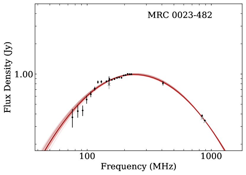
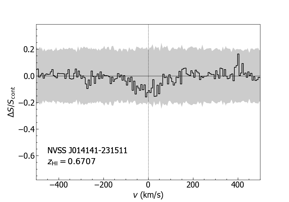
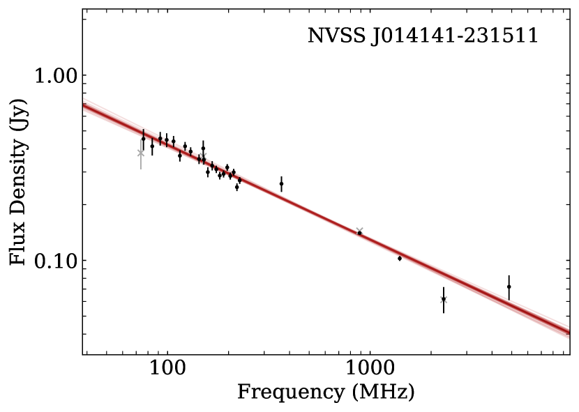
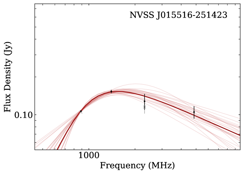
Figure A4: Spectral-line profiles and radio SED fits for: 1. MRC 0023-482 (top), 2. NVSS 014141-231511 (middle), and 3. NVSS J015516-251423 (bottom).

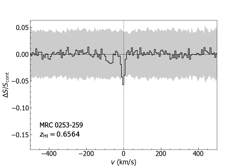
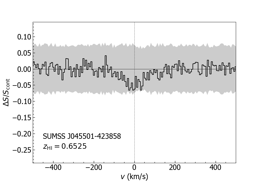
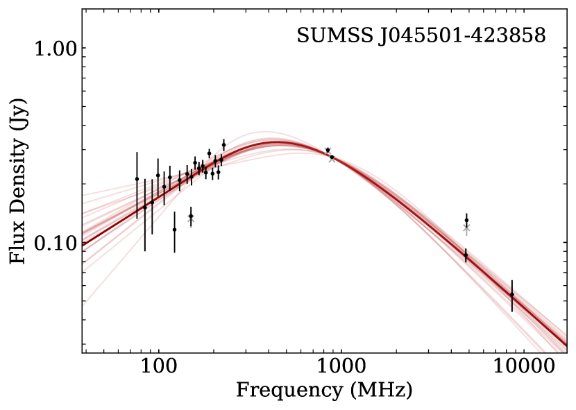
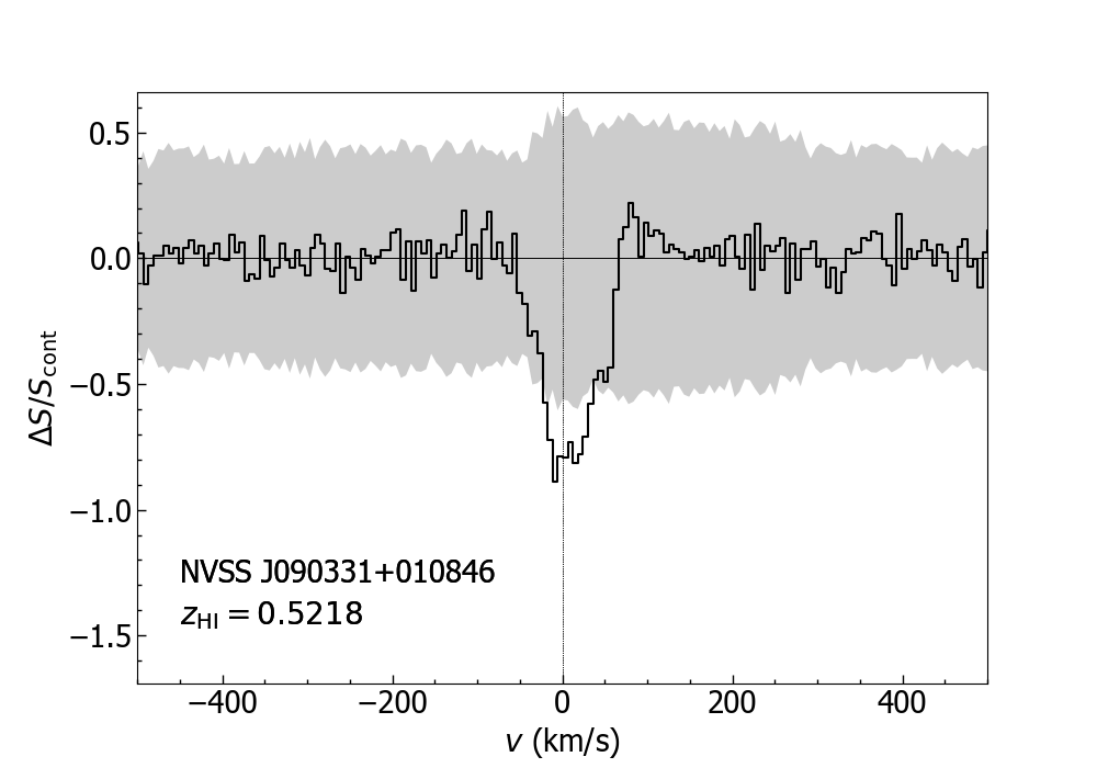
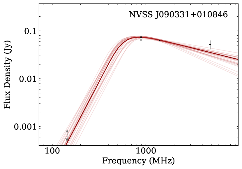
Figure A4: (continued) Spectral-line profiles and radio SED fits for: 4. PKS 0253-259 (top), 5. SUMSS J045501-423858 (middle), and 6. NVSS J090331+010846 (bottom). Note that in the case of NVSS J090331+010846, the SED makes use of an upper limit from LOFAR at 144 MHz (grey arrow) supplied by Callingham & Shimwell (private communication).

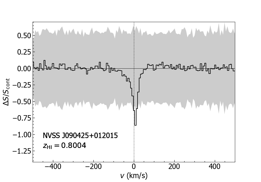
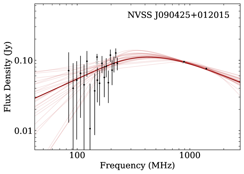
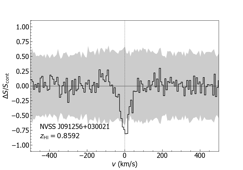
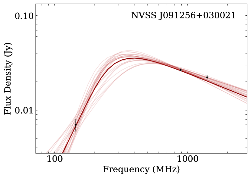
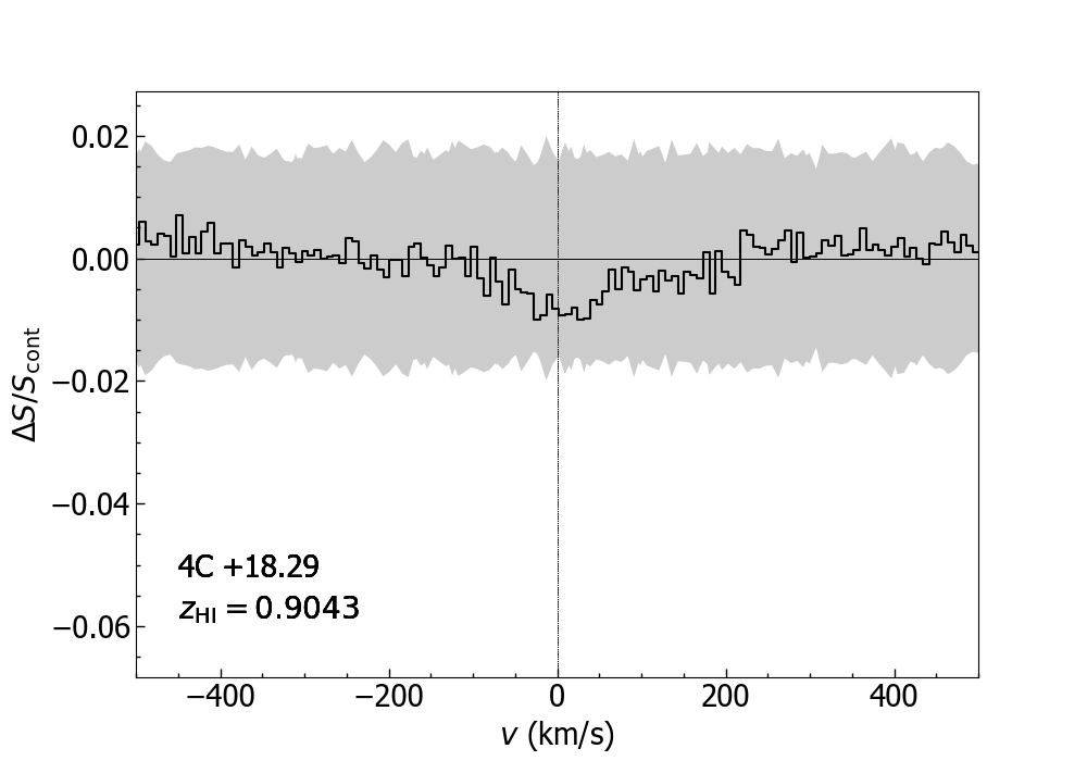
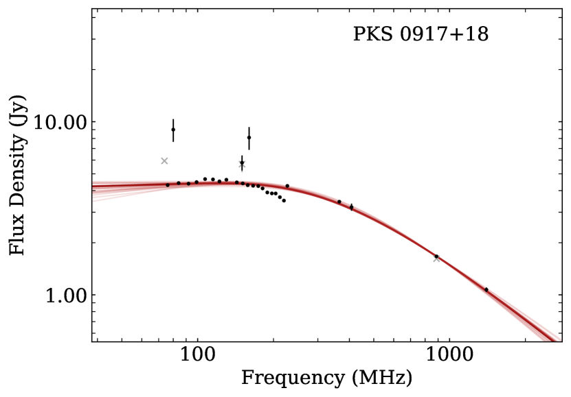
Figure A4: (continued) Spectral-line profiles and radio SED fits for: 7. NVSS J090425+012015 (top), 8. NVSS J091256+030021 (middle), and 9. PKS 0917+18 (bottom). Note that the SED for NVSS J090425+012015 uses LOFAR data at 144 MHz from the LoTSS survey supplied by Callingham (private communication).

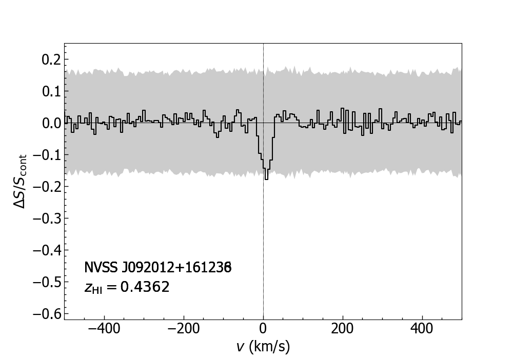
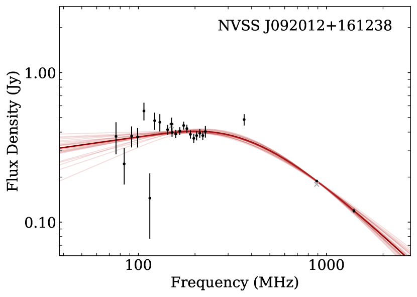
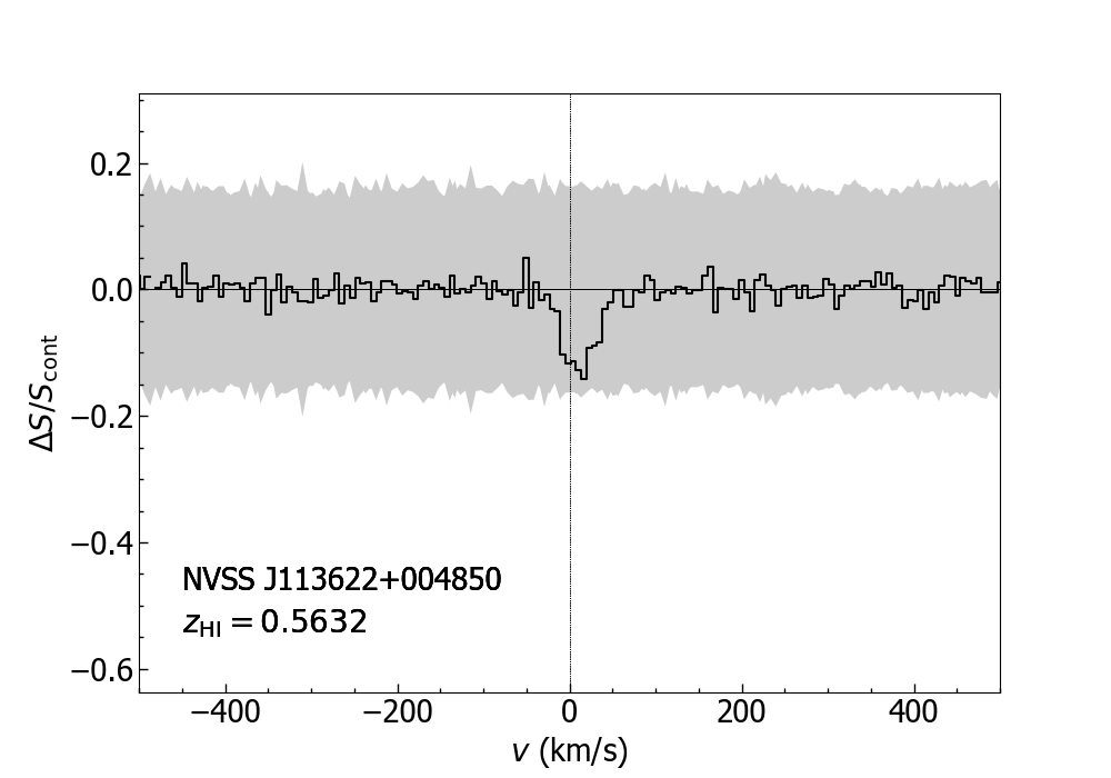
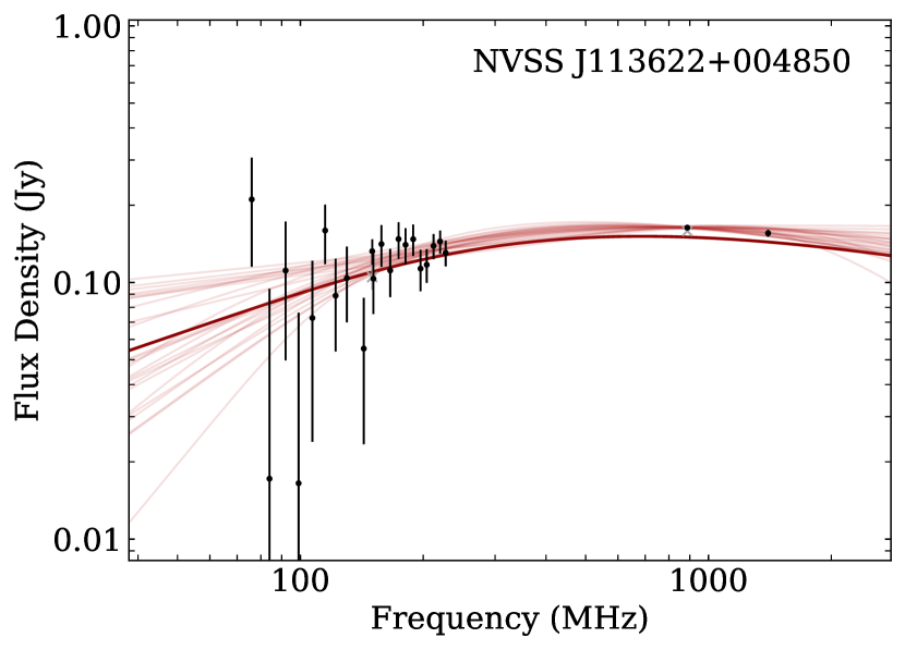
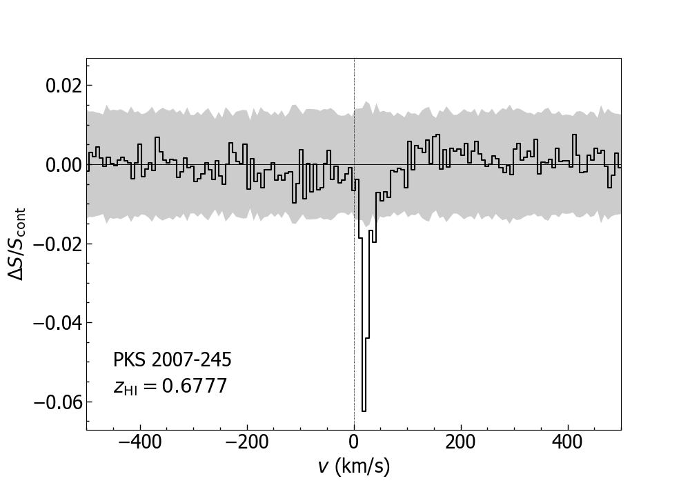
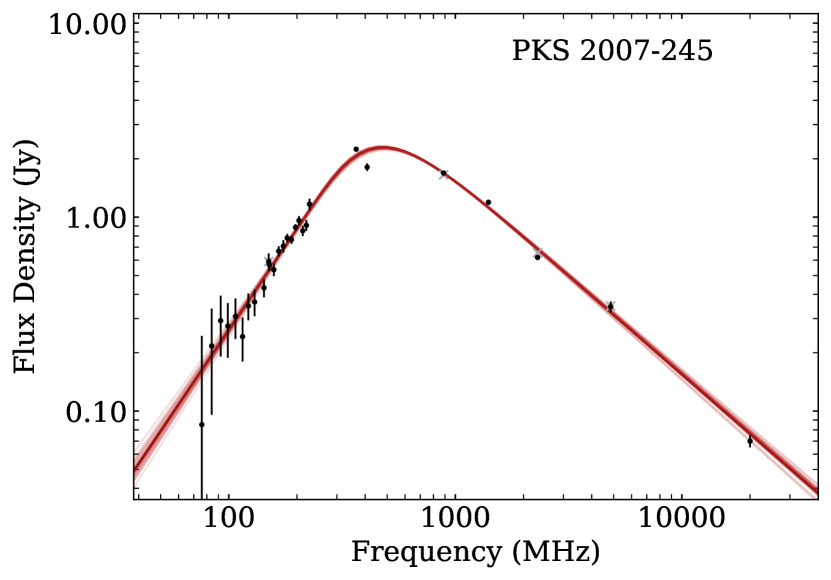
Figure A4: (continued) Spectral-line profiles and radio SED fits for: 10. NVSS J092012+161238 (top), 11.  NVSS J113622+004850 (middle), and 12. PKS 2007-245 (bottom).

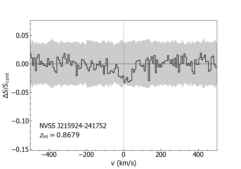
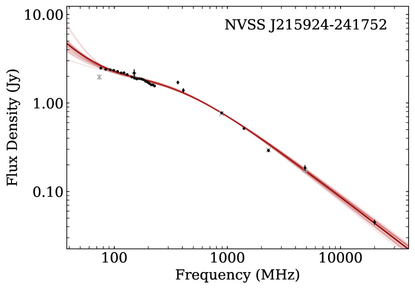
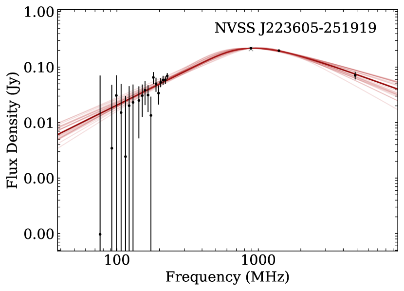
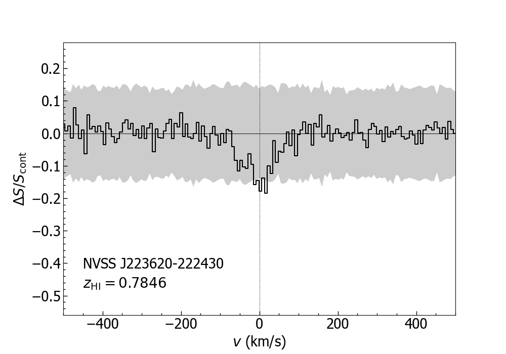
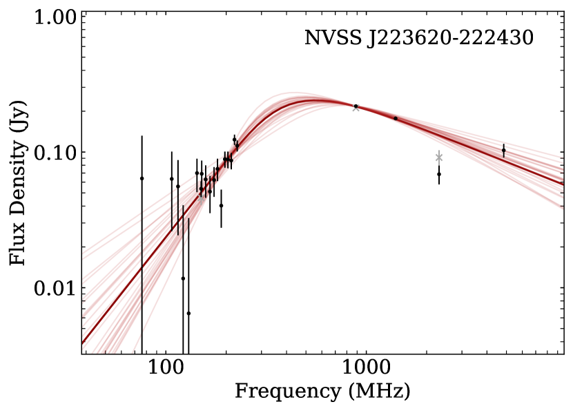
Figure A4: (continued) Spectral-line profiles and radio SED fits for: 13. NVSS J215924-241752 (top), 14.  J223605-251919 (middle), and 15. NVSS J223620-222430 (bottom).

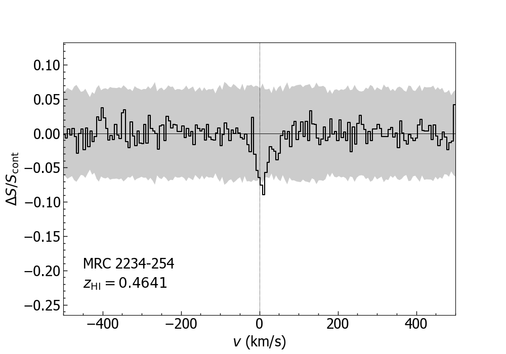
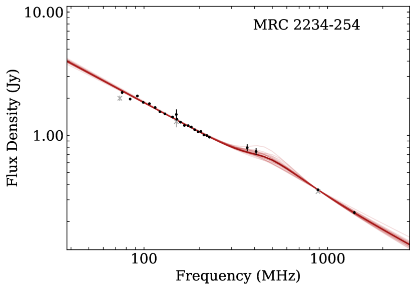
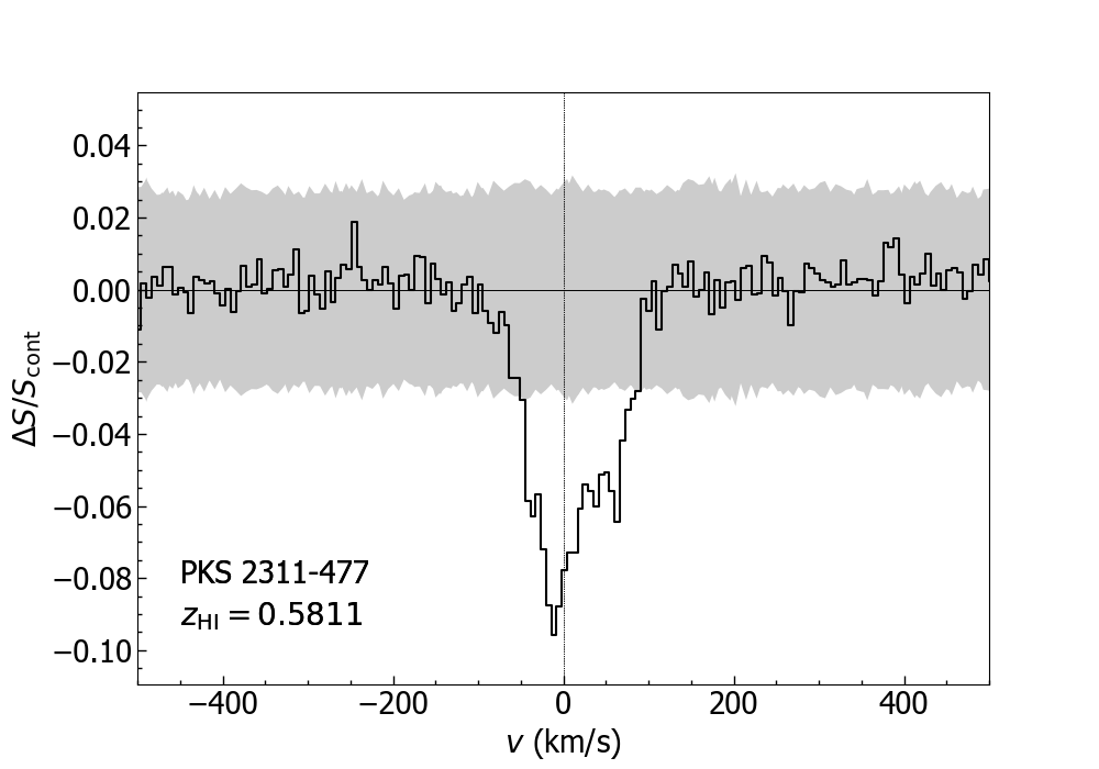
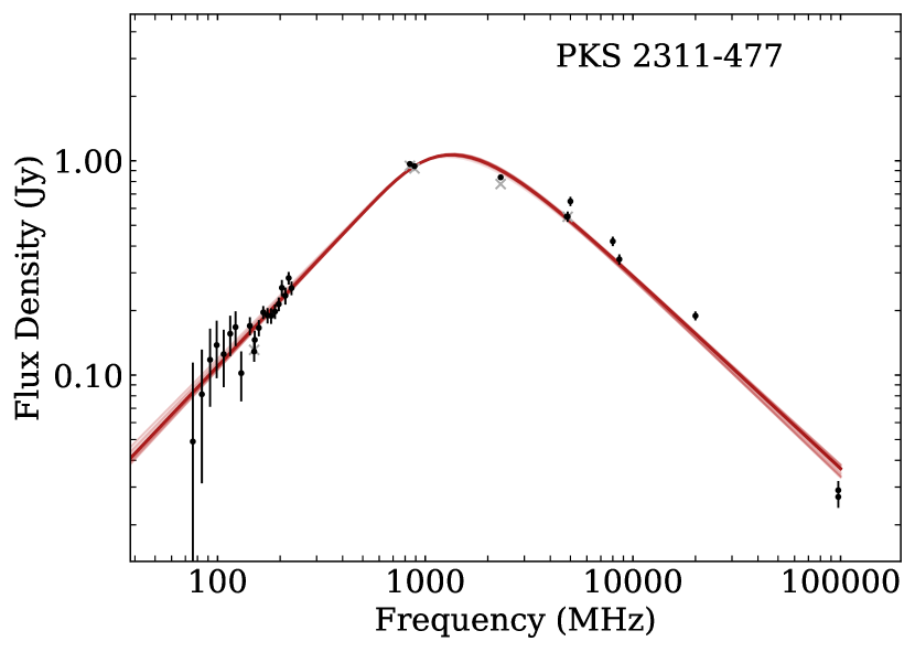
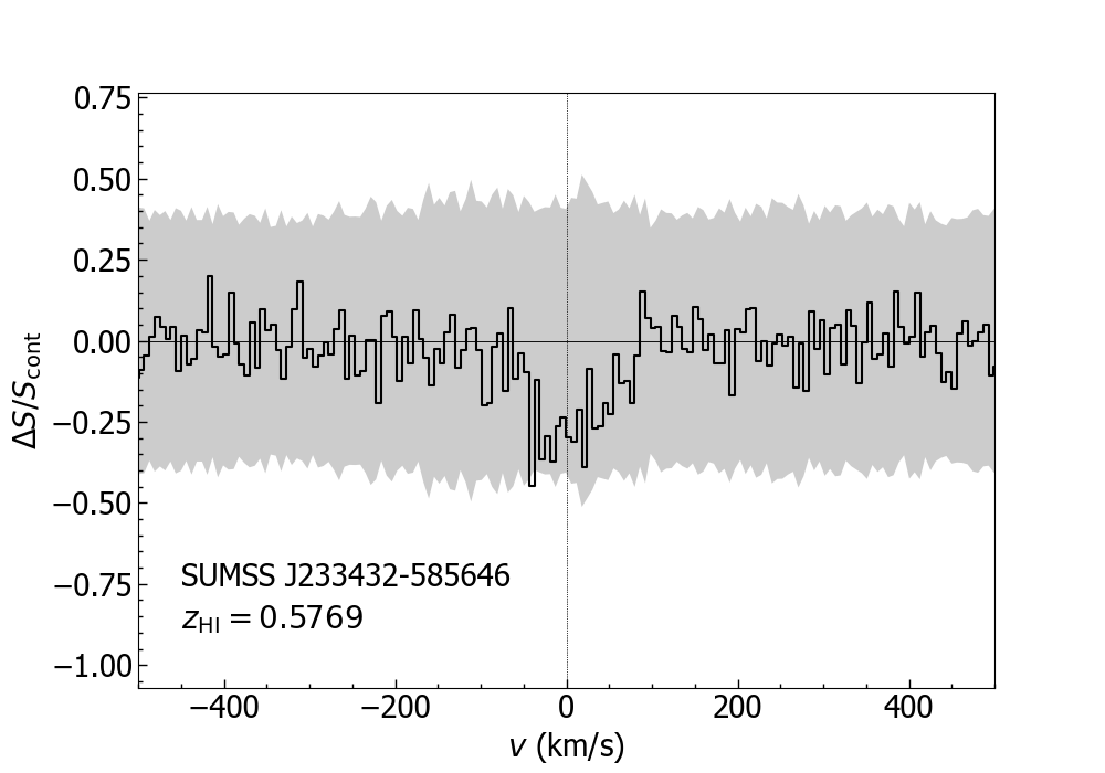
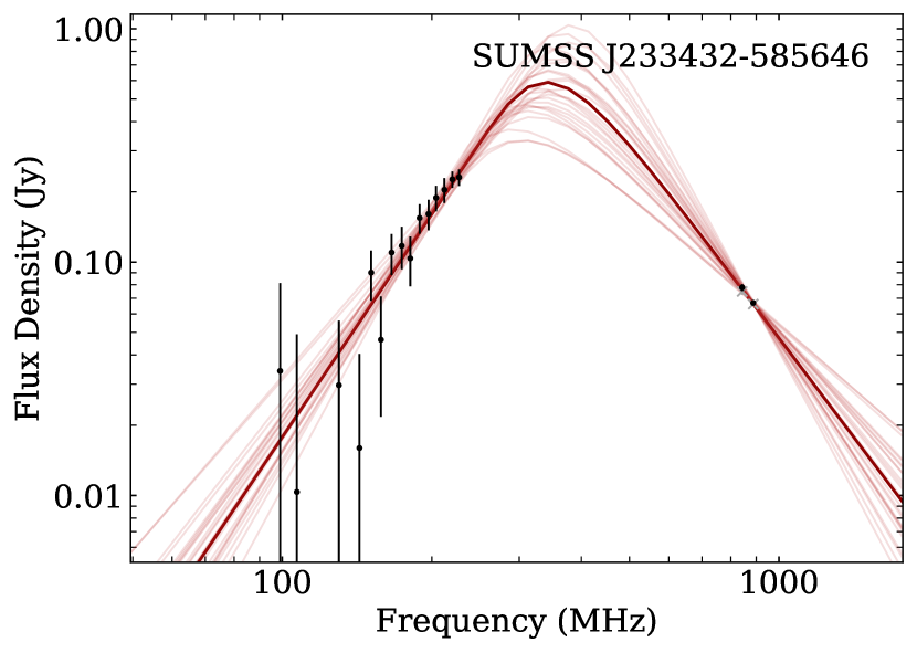
Figure A4: (continued) Spectral-line profiles and radio SED fits for: 16. MRC 2234-254 (top), 17. PKS 2311-477 (middle), and 18. SUMSS J233432-585646 (bottom).

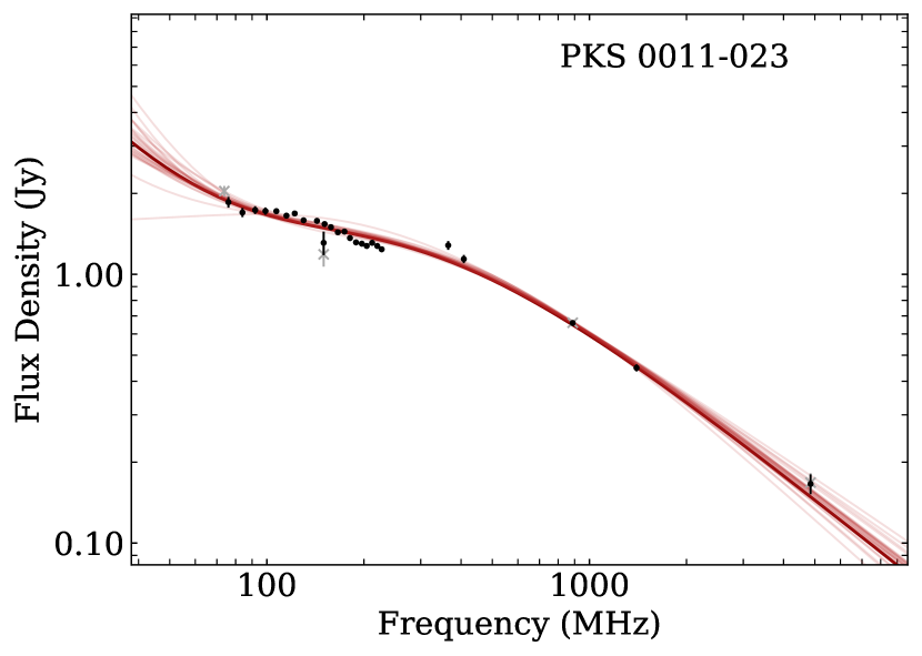
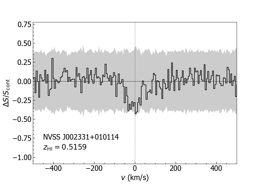
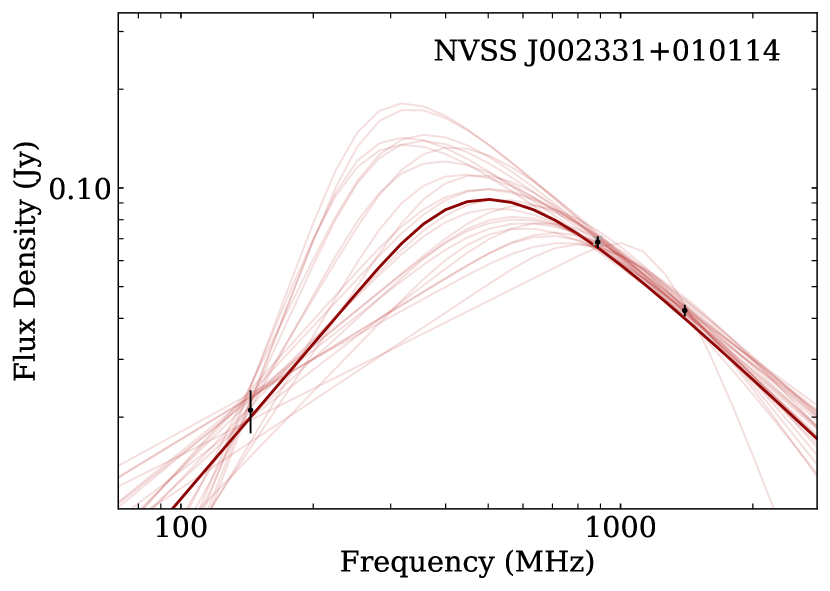
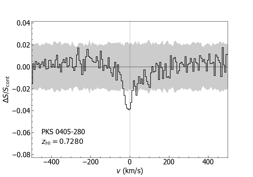
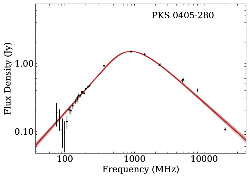
Figure A4: (continued) Spectral-line profiles and radio SED fits for: 19. PKS 0011-023 (top), 20. NVSS J002331+010114 (middle), and 21. PKS 0405-280 (bottom). The SED for NVSS J002331+010114 uses LOFAR data at 144 MHz from the LoTSS survey (private communication with J. Callingham)

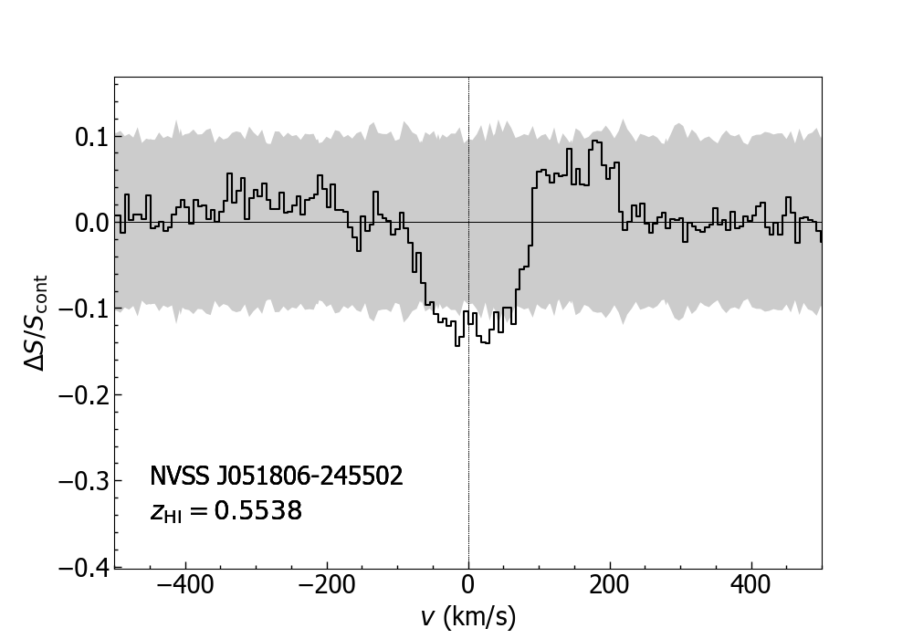
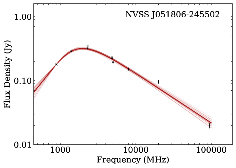
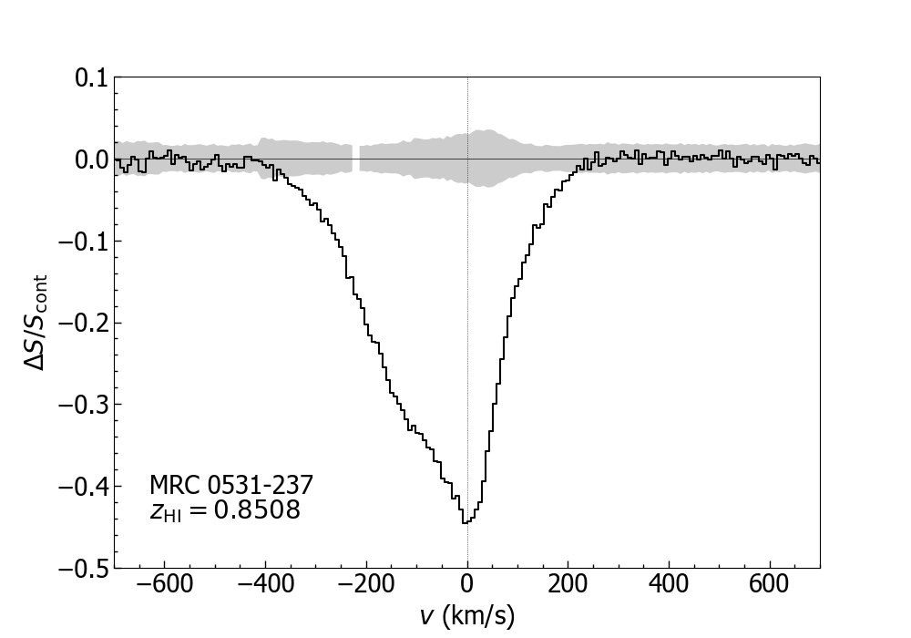
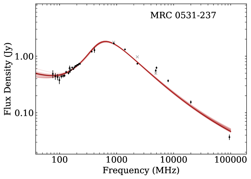
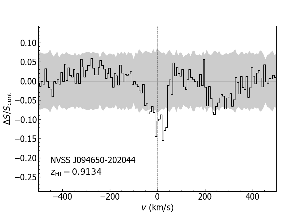
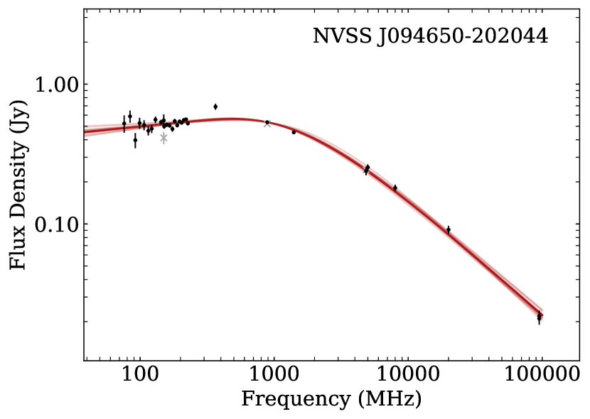
Figure A4: (continued) Spectral-line profiles and radio SED fits for: 22. PKS 0011-023 (top), 23. NVSS J002331+010114 (middle), and 24. PKS 0405-280 (bottom).

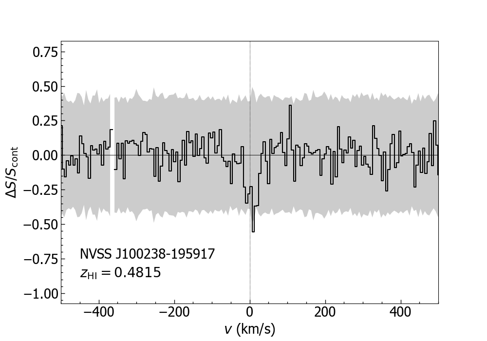
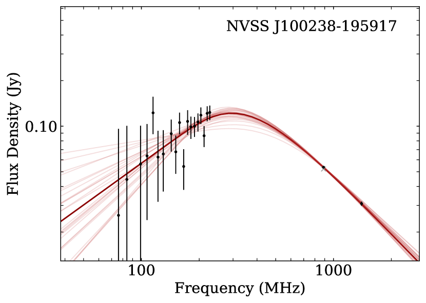
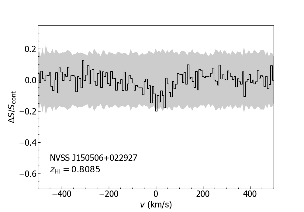
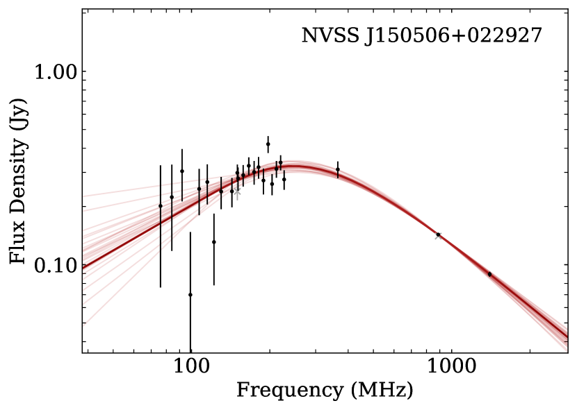
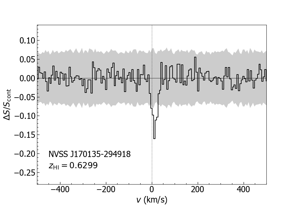
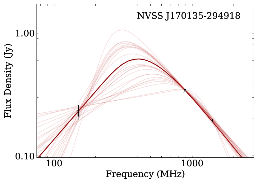
Figure A4: (continued) Spectral-line profiles and radio SED fits for: 25. NVSS J100238-195917 (top), 26. NVSS J150506+022927 (middle), and 27. NVSS J170135-294918 (bottom).

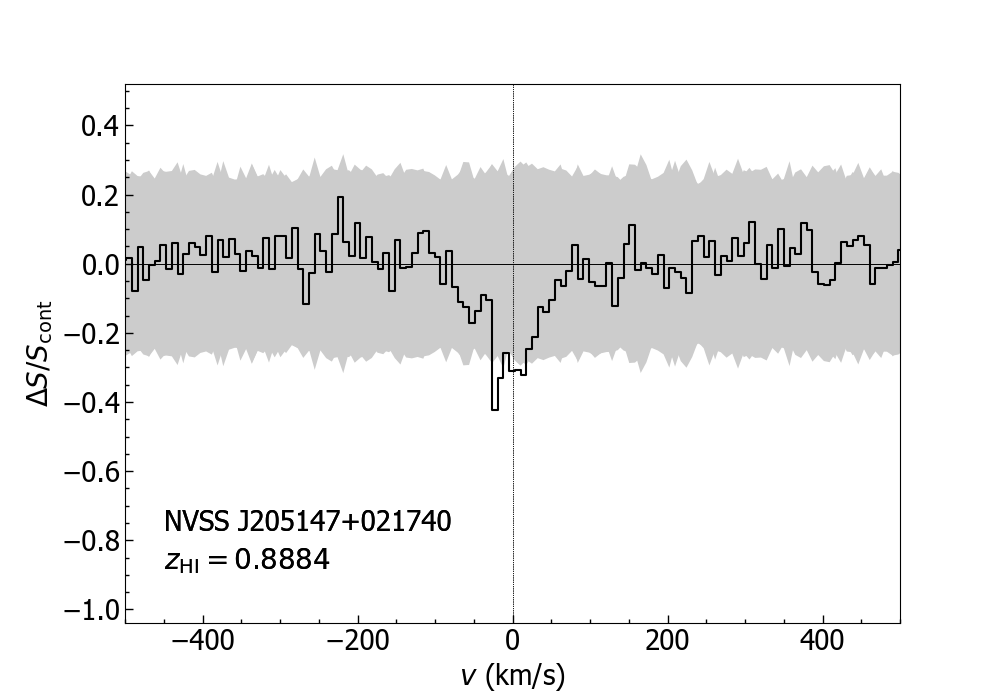
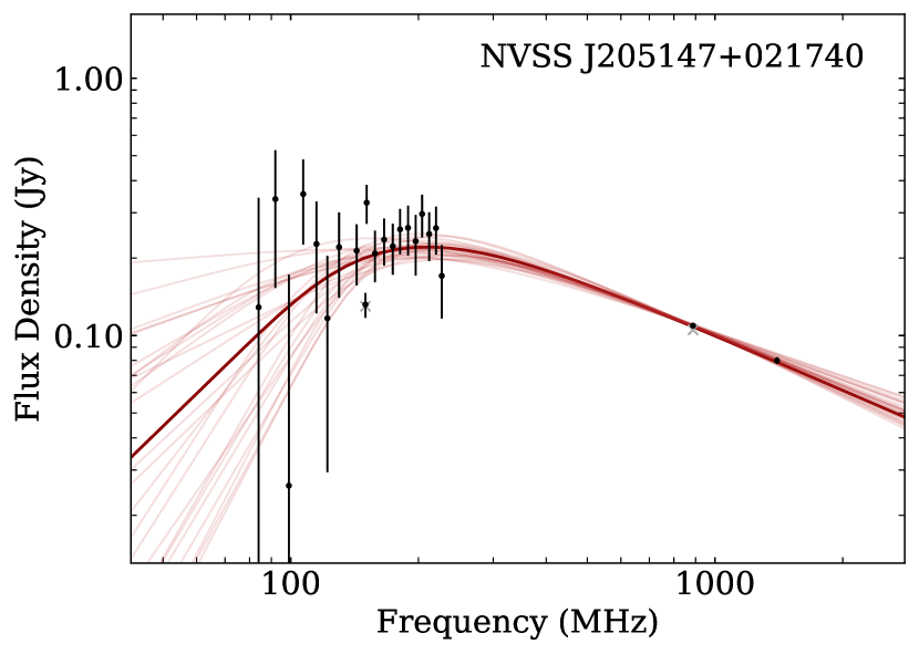
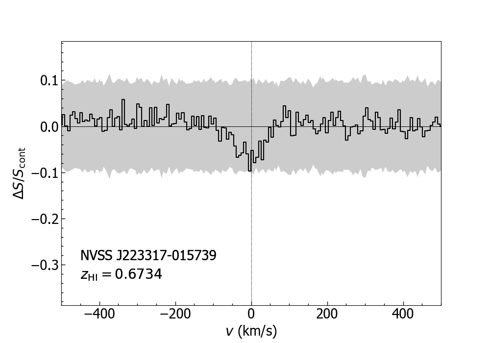
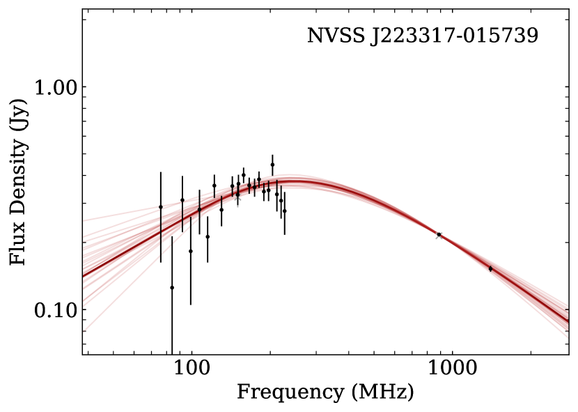
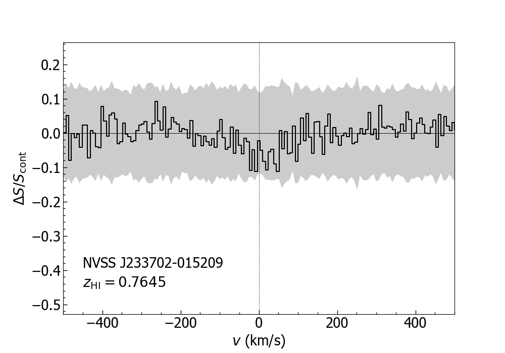
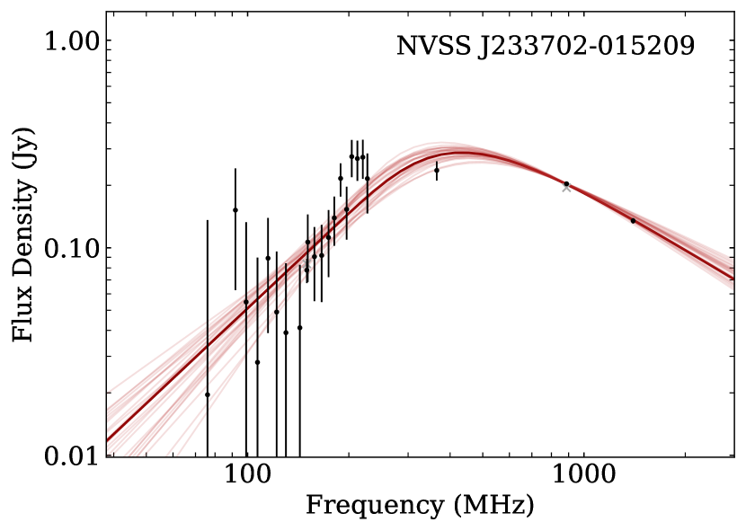
Figure A4: (continued) Spectral-line profiles and radio SED fits for: 28. NVSS 205147+021740 (top), 29. NVSS J223317-015739 (middle), and 30. NVSS J233702-015209 (bottom).

Appendix D Observation logs

Table A1: Log of observations for FLASH Pilot Survey 1.

Field	RA	Dec	Observation		BeamInt	CASDA	rms noise		Notes
	(J2000)		Date	t (h)	(MHz)	SBID	Cont	Line	CASDA validation flag
							(mJy/beam)	(mJy/beam/ch)
(1)	(2)	(3)	(4)	(5)	(6)	(7)	(8)	(9)	(10)
(a) FLASH survey fields observed and released in CASDA
F302P	00 00 00.00	$-25$ 07 47.2	17-Dec-2019	2	5	10850	0.102	5.03	U
F088P	00 21 10.59	$-56$ 18 22.7	20-Apr-2020	2	9	13299	0.088	4.47	U
F303P	00 27 10.19	$-25$ 07 47.2	05-Jan-2020	2	5	11053	0.123	5.97	U
F123P	00 36 55.38	$-50$ 05 45.3	19-Apr-2020	2	9	13290	0.085	4.40	U
F304P	00 54 20.38	$-$25 07 47.2	19-Apr-2020	2	9	13291	0.093	4.62	U
F089P	01 03 31.76	$-$56 18 22.7	20-Apr-2020	2	9	13298	0.090	4.31	U
F306P	01 48 40.75	$-$25 07 47.2	18-Apr-2020	2	9	13281	0.084	4.51	U
F165P	02 13 57.21	$-$43 52 21.4	04-Jul-2020	2	9	..			U
F307P	02 15 50.94	$-$25 07 47.2	17-Apr-2020	2	9	13268	0.085	4.56	U
F308P	02 43 01.13	$-$25 07 47.2	04-Jul-2020	2	9	15212		4.57	U
F309P	03 10 11.32	$-$25 07 47.2	17-Apr-2020	2	9	13269	0.093	4.56	U
F170P	05 01 23.72	$-$43 52 21.4	05-Jul-2020	2	9	15215	0.093		U
F718P	08 43 38.18	$+$18 51 28.9	17-Apr-2020	2	9	13270	0.107	4.63	U
F719P	09 09 49.09	$+$18 51 28.9	17-Apr-2020	2	9	13271	0.106	4.62	U
F607P	10 08 16.55	$+$06 17 42.1	18-Apr-2020	2	9	13284	0.154	4.53	U
F608P	10 33 06.21	$+$06 17 42.1	17-Apr-2020	2	9	13272	0.114	5.06	U
F550P	10 33 06.21	$+$00 00 00.0	20-Apr-2020	2	9	13305	0.106	4.76	U
F194P	18 25 06.98	$-$43 52 21.4	04-Jul-2020	2	9	15208	0.090	4.84	U
F195P	18 58 36.28	$-$43 52 21.4	05-Jul-2020	2	9	..			U
F197P	20 05 34.88	$-$43 52 21.4	04-Jul-2020	2	9	15209	0.093	4.70	U: ducting
F198P	20 39 04.19	$-$43 52 21.4	05-Jul-2020	2	9	..			U
F199P	21 12 33.49	$-$43 52 21.4	04-Jul-2020	2	9	..			U
F351P	22 11 19.25	$-$25 07 47.2	17-Dec-2019	2	5	10849	0.101	4.80	U
F352P	22 38 29.43	$-$25 07 47.2	05-Jan-2020	2	5	11051	0.092	5.07	U
F159P	22 46 09.23	$-$50 05 45.3	17-Apr-2020	2	9	13278	0.089	4.54	U
F120P	22 56 28.24	$-$56 18 22.7	20-Apr-2020	2	9	13297	0.086	4.34	U
F353P	23 05 39.62	$-$25 07 47.2	05-Jan-2020	2	5	11052	0.092	4.98	U
F160P	23 23 04.62	$-$50 05 45.3	04-Sep-2020	2	9	15873	0.093	4.44	U
F354P	23 32 49.81	$-$25 07 47.2	18-Apr-2020	2	9	13279	0.087	4.90	U
F121P	23 38 49.41	$-$56 18 22.7	19-Apr-2020	2	9	13296	0.089	4.50	U
J2022-2507P∗	20 22 38.4	$-$25 07 47.2	22-Apr-2020	2	9	13372	0.090	4.83	U: 305P observed at wrong RA
(b) Fields in the GAMA galaxy survey area
FG9A	08 47 35.59	$+$00 30 00.0	18-Apr-2020	2	9	13285	0.100	4.96	U
FG9A_long	08 47 35.59	$+$00 30 00.0	19-Apr-2020	6	9	13293	0.064	2.75	U
FG9B	09 12 25 24	$+00$ 30 00.0	18-Apr-2020	2	9	13283	0.096	4.63	U
FG9B_long	09 12 25.24	$+$00 30 00.0	07-Jan-2020	6	5	11068	0.078	2.98	U
FG12A	11 47 35.17	$-$00 30 00.0	21-Apr-2020	2	9	13334	0.121	4.75	U
FG12A_long	11 47 35.17	$-$00 30 00.0	20-Apr-2020	6	9	13306	0.079	2.78	U
FG12B	12 12 24.83	$-$00 30 00.0	21-Apr-2020	2	9	13335	0.109	4.78	U
FG12B_long	12 12 24.83	$-$00 30 00.0	22-Apr-2020	6	9	..			Observation failed
FG15A	14 16 33.10	$+$00 30 00.0	21-Apr-2020	2	9	13336	0.114	4.81	U
FG15A_long	14 16 33.10	$+$00 30 00.0	19-Apr-2020	6	9	13294	0.081	2.83	U
FG15B	14 41 22.76	$+$00 30 00.0	17-Apr-2020	2	9	13273	0.110	4.83	U
FG15B_long	14 41 22.6	$+$00 30 00.0	18-Apr-2020	6	9	..			Observation failed

Table A2: Log of observations for FLASH Pilot Survey 2.

Field	RA	Dec	Observation		BeamInt	CASDA	rms noise		Note
	(J2000)		Date	t (h)	(MHz)	SBID	Cont	Line	CASDA validation flag
							(mJy/beam)	(mJy/beam/ch)
(1)	(2)	(3)	(4)	(5)	(6)	(7)	(8)	(9)	(10)
FLASH survey fields observed and released in CASDA
F398∗	18 45 49.00	$-$18 51 45.4	17-Nov-21	2	5	33616	0.082	6.08	Quality Gate, G
F122	00 00 00.00	$-$50 05 45.2	29-Dec-21	2	5	34941	0.079	5.44	U: wobbles, re-obs
F525∗	00 12 24.80	+00 00 00.0	20-Dec-21	2	5	34581	0.105	5.68	U: wobbles, re-obs
F123	00 36 55.30	$-$50 05 45.2	18-Feb-22	2	5	37448	0.087	5.67	G
F526∗	00 37 14.40	+00 00 00.0	26-Dec-21	2	5	34783	0.138	5.80	U: wobbles, ducting, re-obs
F527∗	01 02 04.00	+00 00 00.0	19-Dec-21	2	5	34568	0.138	5.86	U*: ducting
F305	01 21 30.50	$-$25 07 47.2	18-Feb-22	2	5	37449	0.084		G
F528	01 26 53.70	+00 00 00.0	18-Feb-22	2	5	37450	0.128	5.52	G*
F306	01 48 40.70	$-$25 07 47.2	19-Feb-22	2	5	37475	0.114	5.39	G
F529	01 51 43.40	+00 00 00.0	18-Dec-21	2	5	34557	0.098	5.57	U: wobbles, re-obs
F255∗	01 52 56.40	$-$31 23 14.7	15-Jan-22	2	5	35939	0.075	5.23	U: wobbles, re-obs
F530	02 16 33.10	+00 00 00.0	17-Feb-22	2	5	37431	0.105	5.35	G
F256	02 21 10.50	$-$31 23 14.7	20-Dec-21	2	5	34584	0.090	5.62	U: wobbles, re-obs
F531	02 41 22.70	+00 00 00.0	17-Dec-21	2	5	34546	0.098	5.75	U: wobbles, re-obs
F257	02 49 24.70	$-$31 23 14.7	18-Feb-22	2	5	37451	0.082	5.66	G
F532	03 06 12.40	+00 00 00.0	19-Dec-21	2	5	34569	0.113	6.31	U: wobbles, re-obs
F258	03 17 38.80	$-$31 23 14.7	18-Feb-22	2	5	37452	0.074	5.23	G
F533∗	03 31 02.00	+00 00 00.0	15-Jan-22	2	5	35943	0.094	5.68	U: wobbles, re-obs
F310	03 37 21.50	$-$25 07 47.2	17-Feb-22	2	5	37432	0.105	5.61	G
F534	03 55 51.70	+00 00 00.0	18-Dec-21	2	5	34558	0.097	5.55	U: wobbles, re-obs
F311	04 04 31.70	$-$25 07 47.2	18-Feb-22	2	5	37453	0.080	5.28	G
F312	04 31 41.80	$-$25 07 47.2	02-Mar-22	2	5	37797	0.104	5.83	G*
F313	04 58 52.00	$-$25 07 47.2	17-Dec-21	2	5	34547	0.102	5.35	U*: ducting
F314∗	05 26 02.00	$-$25 07 47.2	19-Dec-21	2	5	34570	0.099	5.38	U: wobbles, ducting, re-obs
F545	08 28 57.90	+00 00 00.0	17-Dec-21	2	5	34548	0.105	6.08	U: wobbles, ducting, re-obs
F546	08 53 47.50	+00 00 00.0	18-Dec-21	2	5	34559	0.095	5.37	U: wobbles, re-obs
F719∗	09 09 49.00	+18 51 28.8	18-Dec-21	2	5	34560	0.112	5.88	U: wobbles, ducting, re-obs
F547	09 18 37.20	+00 00 00.0	17-Dec-21	2	5	34549	0.102	5.39	U: wobbles, ducting, re-obs
F377	09 36 00.00	$-$18 51 45.4	19-Dec-21	2	5	34571	0.085	5.45	U: wobbles, ducting, re-obs
F378	10 02 10.90	$-$18 51 45.4	18-Dec-21	2	5	34561	0.096	5.55	U: wobbles, re-obs
F553	11 47 35.10	+00 00 00.0	19-Dec-21	2	5	34572	0.125	5.92	U: wobbles, re-obs
F554	12 12 24.80	+00 00 00.0	28-Dec-21	2	5	34917	0.103		G
F555	12 37 14.40	+00 00 00.0	19-Dec-21	2	5	34562	0.133	6.79	U*
F559∗	14 16 33.10	+00 00 00.0	18-Dec-21	2	5	34551	0.102	5.77	U: wobbles, re-obs
F560	14 41 22.70	+00 00 00.0	19-Dec-21	2	5	34563	0.104	5.48	U: wobbles, re-obs
F561	15 06 12.40	+00 00 00.0	20-Dec-21	2	5	34576	0.105	5.81	U: wobbles, re-obs
F011	16 45 52.80	$-$80 02 36.7	19-Dec-21	2	5	34564	0.098	5.93	U: wobbles, re-obs
F287	16 56 28.20	$-$31 23 14.7	18-Dec-21	2	5	34552	0.132	6.38	U*: ducting
F151	17 50 46.10	$-$50 05 45.2	18-Dec-21	2	5	34553	0.090	5.91	U: wobbles, re-obs
F573	20 04 08.00	+00 00 00.0	18-Dec-21	2	5	34554	0.101	5.46	U*
F574	20 28 57.90	+00 00 00.0	19-Dec-21	2	5	34565	0.098	6.05	U: wobbles, re-obs
F575*	20 53 47.50	+00 00 00.0	19-Dec-21	2	5	34566	0.097	5.80	U*
F575*	20 53 47.50	+00 00 00.0	20-Dec-21	2	5	34577	0.094	5.49	U*
F576	21 18 37.20	+00 00 00.0	20-Dec-21	2	5	34578	0.098	5.50	U: wobbles
F577∗	21 43 26.90	+00 00 00.0	18-Dec-21	2	5	34555	0.098	5.56	U: wobbles, re-obs
F578∗	22 08 16.50	+00 00 00.0	20-Dec-21	2	5	34580	0.097	5.56	U: wobbles, re-obs
F579∗	22 33 06.00	+00 00 00.0	21-Dec-21	2	5	34597	0.099	5.70	U: wobbles, re-obs
F580	22 57 55.80	+00 00 00.0	19-Dec-21	2	5	34567	0.100	6.20	U: wobbles, re-obs
F581∗	23 22 45.50	+00 00 00.0	26-Dec-21	2	5	34781	0.120	5.65	U: wobbles, re-obs
F160∗	23 23 05.00	$-$50 05 45.2	29-Dec-21	2	5	34939	0.078	5.42	U: wobbles, re-obs
F582	23 47 35.10	+00 00 00.0	18-Dec-21	2	5	34556	0.098	5.52	U: wobbles, re-obs

Table A3: Log of observations for FLASH Pilot Survey 2 re-observed fields.

Field	RA	Dec	Observation		BeamInt	CASDA	rms noise		Note
	(J2000)		Date	t (h)	(MHz)	SBID	Cont	Line	CASDA validation flag
							(mJy/beam)	(mJy/beam/ch)
(1)	(2)	(3)	(4)	(5)	(6)	(7)	(8)	(9)	(10)
FLASH survey fields re-observed
F525	00 12 24.80	+00 00 00.0		2	5	42299	0.130	5.52	G
F526	00 37 14.40	$+$00 00 00.0		2	5	42275	0.137	5.52	U*: ducting
F527	01 02 04.14	$+$00 00 00.0		2	5	42300	0.124	5.56	U*: ducting
F255	01 52 56.40	$-$31 23 14.7		2	5	41226	0.080	5.30	G
F255	01 52 56.40	$-$31 23 14.7		2	5	41148	0.101	5.21	U*:
F533	03 31 02.07	+00 00 00.0		2	5	42278	0.112	5.76	U*:
F314	05 26 02.26	$-$25 07 47.2		2	5	41065	0.080	4.90	U*: ducting
F314	05 26 02.26	$-$25 07 47.2		2	5	41061	0.073	5.05	U*:
F719	09 09 49.00	+18 51 28.8		2	5	41084	0.101	4.78	U*: ducting
F719	09 09 49.00	+18 51 28.8		2	5	41066	0.094	4.87	U*: ducting
F559	14 16 33.10	+00 00 00.0		2	5	41085	0.096	5.13	U*: ducting
F559	14 16 33.10	+00 00 00.0		2	5	41068	0.092	5.06	U*: ducting
F398	18 45 49.00	$-$18 51 45.4		2	5	41071	0.082	5.99	G
F398	18 45 49.00	$-$18 51 45.4		2	5	41050	0.084	6.21	U*: ducting
F577	21 43 26.90	+00 00 00.0		2	5	42296	0.109	5.55	U*: ducting
F578	22 08 16.50	+00 00 00.0		2	5	42297	0.122	5.47	U*: ducting
F578	22 08 16.50	+00 00 00.0		2	5	43424	0.100	5.66	G
F579	22 33 06.00	+00 00 00.0		2	5	42298	0.118	5.55	U*: ducting
F581	23 22 45.50	+00 00 00.0		2	5	41105	0.350	6.36	U*:
F581	23 22 45.50	+00 00 00.0		2	5	41072	0.094	5.22	U*: ducting
F581	23 22 45.50	+00 00 00.0		2	5	41225	0.112	5.75	U*:
F581	23 22 45.50	+00 00 00.0		2	5	41184	0.106	5.80	U*
F160	23 23 04.62	$-$50 05 45.3		2	5	42323	0.100	5.66	U*: ducting
F160	23 23 04.62	$-$50 05 45.3		2	5	43426	0.075	5.18	G

Appendix E Linefinder results for individual SBIDs

Table A4: Original FLASHfinder results; (1) ID; (2) Selavy name; (3) Component ID; (4) Field name; (5) Continuum flux density for this component; (6) H i redshift; (7) Peak optical depth; (8) Integrated optical depth; (9) Linewidth; (10) ln (B); (11) Notes (F=close to field edge; N=Individual Note in Appendix B)

ID	Selavy ID	Component	FLASH	Scont.	$z_{\rm HI}$	$\tau_{\rm peak}$	$\tau_{\rm int}$	Linewidth	ln (B)	Notes
		name	field	(Jy)			(km s-1)	(km s-1)
(1)	(2)	(3)	(4)	(5)	(6)	(7)	(8)	(9)	(10)	(11)
(a) New pilot survey detections
1	SB13290 19a	J002604-475618	123P	0.400	0.6745	..	..	..	..	N
1	SB37448 19a	J002604-475617	123	0.358	0.6746	0.081	4.07	50.3	44.4
2	SB13281 64a	J014141-231510	306P	0.138	0.6707	0.161	20.02	124.8	77.5
2	SB37475 67a	J014141-231508	306	0.136	0.6706	0.100	14.27	143.0	34.0
3	SB13281 103a	J015516-251423	306P	0.099	0.7251	1.802	95.66	53.1	1174.7
3	SB37475 95a	J015516-251422	306	0.106	0.7251	1.891	95.39	50.5	1065.4
4	SB13269 2a/2b	J025544-254741	309P	0.604	0.6564	0.052	1.08	20.7	32.4	F
4	SB15212 9a	J025544-254739	308P	0.805	0.6564	0.051	1.07	21.3	74.7
5	SB15215 27a	J045501-423858	170P	0.288	0.6525	0.051	7.38	146.4	83.3
6	SB13283 228a	J090331+010847	G09B	0.053	0.5218	3.079	187.78	60.9	466.2
6	SB34559 191a	J090331+010846	546	0.070	0.5218	1.344	82.19	61.1	485.4
7	SB13283 91a	J090425+012015	G09B	0.087	0.8004	0.924	36.80	39.9	303.6
7	SB34549 120a	J090425+012013	547	0.095	0.8004	1.421	28.07	19.4	35.6	F
7	SB34559 117a	J090425+012013	546	0.080	0.8004	1.588	46.98	29.5	238.7
8	SB11068 403a	J091256+030020	G09B_long	0.033	0.8590	1.253	64.97	51.7	103.1
9	SB13271 2a	J092011+175324	719P	1.752	0.9040	0.009	1.90	218	65.6
9	SB41066 3a	J092011+175324	719	1.800	0.9044	0.01	1.14	119.6	53.7
10	SB13271 57a	J092012+161239	719P	0.105	0.4362	0.082	7.37	89.2	46.9
10	SB34560 55a	J092012+161236	719	0.206	0.4362	0.139	3.28	23.8	14.9
10	SB41066 56a	J092012+161238	719	0.202	0.4362	0.169	4.88	29.1	63.3
11	SB13334 64a	J113622+004850	G12A	0.130	0.5630	0.130	6.71	51.8	28.9
11	SB13306 65a	J113622+004851	G12A_long	0.165	0.5630	0.142	7.52	52.9	158.9
11	SB34572 65a	J113622+004850	553	0.166	0.5630	0.083	3.74	45.0	13.3
12	SB13372 1a	J201045-242545	J2022-2507	1.827	0.6778	0.007	1.36	186.2	110.0
13	SB10849 8a	J215924-241752	351P	0.806	0.8680	0.028	2.68	94.5	50.3
14	SB11051 35a	J223605-251918	352P	0.215	0.4974	0.415	11.27	27.2	512.6
15	SB11051 38a	J223619-222429	352P	0.207	0.7846	0.158	15.35	97.4	113.6
16	SB11051 17a	J223722-251003	352P	0.343	0.4641	0.072	3.06	42.7	58.4
17	SB15873 5a	J231351-472911	160P	1.044	0.5811	0.078	8.80	113.0	1706.2
17	SB34939 5a	J231351-472911	160	0.952	0.5811	0.072	7.89	110.3	945.6
18	SB13296 158a	J233432-585646	121P	0.074	0.5769	0.366	37.43	101.6	65.4
19	SB34581 9a	J001425-020556	525	0.694	0.6785	0.216	7.90	36.6	1237.4	N
20	SB34581 149a	J002331+010114	525	0.067	0.5159	0.432	32.4	74.7	76.9
21	SB37453 1a	J040757-275705	311	1.278	0.7280	0.032	2.97	94.0	254.5
22	SB34570 50a	J051805-245502	314	0.195	0.5538	0.141	16.04	114	272.3
22	SB41061 50a	J051805-245502	314	0.180	0.5538	0.156	18.61	119	451.8
22	SB41065 51a	J051805-245502	314	0.184	0.5538	0.169	18.45	109.1	500.7
23	SB41061 1a	J053354-234430	314	1.742	0.8507	0.415	81.7	197	36242.7
23	SB41065 1a	J053354-234430	314	1.751	0.8508	0.359	71.48	199.1	37146.9
24	SB34571 8a	J094650-202045	377	0.550	0.9134	0.135	10.6	78.2	249.2
25	SB34561 188a	J100238-195919	378	0.057	0.4815	0.5	17.16	34.2	35.2
26	SB34576 62a	J150506+022928	561	0.150	0.8085	0.112	11.96	107.4	35.4
27	SB34552 19a	J170135-294917	287	0.403	0.6299	0.149	4.44	29.9	144.0
28	SB34566 100a	J205147+021738	575	0.115	0.8883	0.361	30.68	84.9	123.9
28	SB34577 94a	J205147+021740	575	0.107	0.8884	0.383	28.9	75.6	125.3
29	SB34597 47a	J223317-015739	579	0.231	0.6734	0.076	5.45	71.7	43.8
29	SB42298 45a	J223317-015739	579	0.239	0.6733	0.073	6.48	89.2	56.3
30	SB34556 46a	J233703-015210	582	0.232	0.7645	0.072	9.24	128.4	34.3
(b) Pilot 2 observations of known strong absorption lines
31	SB34564 2a	J161749-771717	11	4.184	0.4502	0.03	1.69	55.7	1639.0
32	SB34553 1a	J174425-514442	151	7.788	..	..	..	..	..	N
33	SB33616 1a	J183339-210339	398	11.888	0.8851	0.053	9.66	183.9	20852.0