Bordered Floer homology, handlebody detection, and compressing diffeomorphisms

Abstract.

We show that, up to connected sums with integer homology $L$-spaces, bordered Floer homology detects handlebodies, as well as whether a mapping class extends over a given handlebody or compression body. Using this, we combine ideas of Casson-Long with the theory of train tracks to give an algorithm using bordered Floer homology to detect whether a mapping class extends over any compression body.

1. Introduction

To apply a numerical or algebraic invariant to topological problems, it is helpful to know what geometric information the invariant contains. For Heegaard Floer homology, some of the most useful information comes from its famous detection properties: Ozsváth and Szabó’s theorems that it detects the genus of knots and the Thurston norm of 3-manifolds [OSz04a] and Ni’s theorems that it detects fiberedness of knots and 3-manifolds [Ni07, Ni09] (see also [Ghi08]). A useful cousin of these properties is that various twisted forms of Heegaard Floer homology detect the existence of homologically essential 2-spheres [HN13, AL19].

This last result extends easily to show that twisted Heegaard Floer homology can also be used to detect the presence of homologically linearly independent 2-spheres (Lemma 5.6, below). In this paper, we use that extension to give two new phenomena that bordered Heegaard Floer homology detects: it detects handlebodies (Theorem 1.1), and also whether a diffeomorphism extends over a given handlebody or compression body (Theorem 1.3). A related question is whether a diffeomorphism extends over any handlebody. Casson and Long give an algorithm for answering this in the 1980s [CL85]. (One reason for interest was a theorem of Casson and Gordon that the monodromy of a fibered ribbon knot extends over a handlebody [CG83].) We modify their algorithm to show that bordered-sutured Floer homology can be used to detect whether a diffeomorphism extends over some compression body, and give explicit bounds on the complexity of the bimodules involved (Theorem 1.5). In particular, the proof involves replacing some bounds in terms of the lengths of geodesics with bounds in terms of train tracks and giving a connection between train track splitting sequences and bordered-sutured bimodules associated to mapping classes, both of which may be of independent use.

We state these results in a little more detail, starting with detection of handlebodies:

Theorem 1.1.

Let $Y$ be an irreducible homology handlebody. Fix $\phi\nobreak\mskip 2.0mu\mathpunct{}\nonscript\mkern-3.0mu{:}\penalty 300\mskip 6.0mu plus 1.0muF\to\partial Y$ making $Y$ into a bordered $3$-manifold and let ${}^{\mathcal{A}(F)}\mskip-1.80002mu\underline{\widehat{\mathit{CFDA}}}(\mathit{Id})_{\mathcal{A}(F)}$ be the twisted identity bimodule of $F$. Then the support of

$$\operatorname{Mor}_{\mathcal{A}(F)}\bigl{(}{}^{\mathcal{A}(F)}\mskip-1.80002mu\widehat{\mathit{CFD}}(Y),{}^{\mathcal{A}(F)}\mskip-1.80002mu\underline{\widehat{\mathit{CFDA}}}(\mathit{Id})_{\mathcal{A}(F)}\boxtimes{}^{\mathcal{A}(F)}\mskip-1.80002mu\widehat{\mathit{CFD}}(Y)\bigr{)}$$

over $\mathbb{F}_{2}[H_{2}(Y,F)]$ is $0$-dimensional if and only if $Y$ is a handlebody.

Corollary 1.2.

Let $Y$ be a bordered $3$-manifold so that $\widehat{\mathit{CFD}}(Y)$ is homotopy equivalent to $\widehat{\mathit{CFD}}(H,\phi)$ for some bordered handlebody $H$, as (relatively) graded type $D$ structures. Then $Y$ is a connected sum of a handlebody and an integer homology sphere $L$-space.

Given a surface $\Sigma$, a $3$-manifold $Y$ with $\Sigma\subset\partial Y$, and a homeomorphism $\psi\nobreak\mskip 2.0mu\mathpunct{}\nonscript\mkern-3.0mu{:}\penalty 300\mskip 6.0mu plus 1.0mu\Sigma\to\Sigma$, $\psi$ extends over $Y$ if there is a homeomorphism $\Psi\nobreak\mskip 2.0mu\mathpunct{}\nonscript\mkern-3.0mu{:}\penalty 300\mskip 6.0mu plus 1.0muY\to Y$ so that $\Psi|_{F}=\psi$. With a little more work, the techniques used to prove Theorem 1.1 also show that bordered Floer homology detects whether a homeomorphism extends over a given handlebody or compression body:

Theorem 1.3.

Let $C$ be a compression body with outer boundary $\Sigma$ and $k$ components of its inner boundary (none of which are spheres), and let $\psi\nobreak\mskip 2.0mu\mathpunct{}\nonscript\mkern-3.0mu{:}\penalty 300\mskip 6.0mu plus 1.0mu\Sigma\to\Sigma$ be a homeomorphism. Let $g^{\prime}$ be the sum of the genera of the components of the inner boundary of $C$. Make $C$ into a special bordered-sutured manifold with outer bordered boundary $F$, inner bordered boundary $F^{\prime}$, and $m$ sutures on the inner boundary, and choose a strongly based representative for $\psi$ (i.e., a representative respecting the sutured structure on $\partial F$). Then $\psi$ extends over $C$ if and only if $\psi$ preserves the kernel of the map $H_{1}(\Sigma)\to H_{1}(C)$ and the support of

(1.4) $$\operatorname{Mor}_{\mathcal{A}(F)}\bigl{(}{}^{\mathcal{A}(F^{\prime}),\mathcal{A}(F)}\mskip-1.80002mu\mathit{BSD}(C),{}^{\mathcal{A}(F)}\mskip-1.80002mu\mathit{BSDA}(\psi)_{\mathcal{A}(F)}\boxtimes{}^{\mathcal{A}(F),\mathcal{A}(F^{\prime})}\mskip-1.80002mu\underline{\mathit{BSD}}(C)\bigr{)}$$

over $\mathbb{F}_{2}[H_{2}(C,F\cup F^{\prime})]$ is $(2g^{\prime}+k-m)$-dimensional.

In particular, if there is one suture on each inner boundary component, then the question is whether the support is $2g^{\prime}$-dimensional.

If $C$ is a handlebody, Formula (1.4) reduces to whether

$$\dim\operatorname{Supp}\operatorname{Mor}_{\mathcal{A}(F)}\bigl{(}{}^{\mathcal{A}(F)}\mskip-1.80002mu\widehat{\mathit{CFD}}(C),{}^{\mathcal{A}(F)}\mskip-1.80002mu\widehat{\mathit{CFDA}}(\psi)_{\mathcal{A}(F)}\boxtimes{}^{\mathcal{A}(F)}\mskip-1.80002mu\underline{\widehat{\mathit{CFD}}}(C)\bigr{)}=0.$$

This can also be interpreted as

$$\dim\operatorname{Supp}\operatorname{Mor}_{\mathcal{A}(F)}\bigl{(}{}^{\mathcal{A}(F)}\mskip-1.80002mu\widehat{\mathit{CFD}}(C),{}^{\mathcal{A}(F)}\mskip-1.80002mu\underline{\widehat{\mathit{CFDA}}}(\mathit{Id})_{\mathcal{A}(F)}\boxtimes{}^{\mathcal{A}(F)}\mskip-1.80002mu\widehat{\mathit{CFDA}}(\psi)_{\mathcal{A}(F)}\boxtimes{}^{\mathcal{A}(F)}\mskip-1.80002mu\widehat{\mathit{CFD}}(C)\bigr{)},$$

as in Theorem 1.1.

Since the bordered Floer algebras categorify the exterior algebra on $H_{1}(F)$ or, more precisely, bordered Floer homology categorifies the Donaldson TQFT [HLW17, Pet18], the bordered condition in Theorem 1.3 is in some sense a categorification of the obvious necessary condition that $\psi$ preserve the kernel of $H_{1}(\Sigma)\to H_{1}(C)$. So, like with the Thurston norm, Floer homology detects a phenomenon which classical topology merely obstructs. There are other interesting obstructions to partially extending diffeomorphisms over 3-manifolds with boundary, e.g., in terms of laminations [BJM13]; in light of the third part of the paper, it might be interesting to compare the two kinds of techniques.

Theorems 1.1 and 1.3 are effective: the bordered invariants are computable [LOT18] (see also [Zha]), and the dimension of the support of these modules can also be computed (Section 5.3).

A related problem to asking whether a given homeomorphism $\psi$ of $\Sigma$ extends over a given compression body filling of $\Sigma$ is to ask if $\psi$ extends over any compression body filling of $\Sigma$. In 1985, Casson-Long showed that this problem is algorithmic, using a bound in terms of how $\psi$ interacts with geodesics on $\Sigma$, which they call the intercept length [CL85]. In particular, they show that if $\psi$ extends over a handlebody, it also extends over a compression body containing a disk whose boundary is relatively short (with respect to a metric on $\Sigma$). Combining some of their ideas with results about train tracks, we show that if $\psi$ extends over a handlebody then $\psi$ extends over a compression body whose bordered Floer bimodule is relatively small. More precisely:

Theorem 1.5.

Let $\psi\nobreak\mskip 2.0mu\mathpunct{}\nonscript\mkern-3.0mu{:}\penalty 300\mskip 6.0mu plus 1.0mu\Sigma\to\Sigma$ be a mapping class of a closed surface $\Sigma$ with genus $g$. Let $(m_{i,j})$ be the incidence matrix for $\psi$ with respect to some train track $\tau$ carrying $\psi$, $\kappa$ be the number of connected components of $\Sigma\setminus\tau$, $s$ be the number of switches of $\tau$, and $M(\psi)$ be as in Formula (8.11). Then there is a bordered Heegaard diagram $\mathcal{H}$ for a compression body $C_{\mathcal{H}}$ with boundary $\Sigma$ so that $\psi$ extends over $C_{\mathcal{H}}$ and $\mathcal{H}$ has at most

$$(20(g+s)-18)^{s}\left((2M(\psi))^{2g}+(2M(\psi)+8)^{2(g+s-1)}\right)$$

many generators.

(This is re-stated and proved as Theorem 8.15.)

Corollary 1.6.

Bordered-sutured Floer homology gives an algorithm to test whether $\psi$ extends over some compression body, or over some handlebody.

The proof of Theorem 1.5 has several ingredients. One is a construction of bordered Heegaard diagrams from trivalent train tracks. Another is to define a notion of length of a curve in terms of its intersections with stable and unstable train tracks for $\psi$, and to use Agol’s periodic splitting sequences to give bounds on this length for some curve bounding a disk in the compression body.

Convention 1.7.

Because we are working mostly with compression bodies and handlebodies, throughout this paper by 3-manifold we mean a compact, connected, orientable 3-manifold with boundary; when 3-manifolds are required to be closed, we will say that explicitly.

This paper is organized as follows. Section 2 is a quick review of the theory of train tracks for pseudo-Anosov maps, collecting the material needed to prove Theorem 1.5. Section 3 has some general results about compression bodies and decompositions of 3-manifolds along spheres, needed for Theorems 1.1 and 1.3. Terminology about compression bodies is also explained in Section 3. Section 4 recalls twisted Heegaard Floer homology and sutured Floer homology and untwisted bordered-sutured Floer homology, and then introduces twisted bordered-sutured Floer homology. It also introduces the notion of special bordered-sutured manifolds. None of the material in that section will be surprising to experts, but some has not yet appeared in the literature. Section 5 starts by recalling the definition of the support and then proves Theorem 1.1. It also indicates what we mean by the support of the bordered invariants (needed for later sections) and discusses how one can compute these supports. The proof of Theorem 1.3 is in Section 6. Section 7 connects the material from Sections 2 and 4, showing how train tracks give arc diagrams and splitting sequences give factorizations of mapping classes into arcslides. Section 8 builds on these ideas to prove Theorem 1.5 and Corollary 1.6.

Acknowledgments

We thank Nick Addington, Mark Bell, Spencer Dowdall, Dave Gabai, Tye Lidman, Dan Margalit, and Lee Mosher for helpful conversations. We also thank the Simons Laufer Mathematical Sciences Institute for its hospitality in Fall 2022, while much of this work was conducted.

2. Background on pseudo-Anosov maps and train-tracks

Let $\Sigma$ be an oriented surface. For the most part, this section follows [PH92], so we assume $\Sigma$ is not the once punctured torus. A diffeomorphism $\psi$ of $\Sigma$ is called pseudo-Anosov if there exist transverse measured foliations $(\mathcal{F}^{s},\mu_{s})$ and $(\mathcal{F}^{u},\mu_{u})$ on $\Sigma$ and a real number $\lambda>1$ such that $\mathcal{F}^{s}$ and $\mathcal{F}^{u}$ are preserved by $\psi$, while the measures $\mu_{s}$ and $\mu_{u}$ are multiplied by $1/\lambda$ and $\lambda$, respectively. The constant $\lambda(\psi)=\lambda$ is called the dilatation number of $\psi$.

Thurston introduced measured train tracks as combinatorial tools to encode the measured foliations $(\mathcal{F}^{s},\mu_{s})$ and $(\mathcal{F}^{u},\mu_{u})$. A train track $\tau\subset\Sigma$ is an embedded graph on $\Sigma$ satisfying the following conditions:

1. Each edge is $C^{1}$ embedded, and at each vertex there is a well-defined tangent line to all of the edges adjacent to it as in Figure 1.

2. For every connected component $S$ of $\Sigma\setminus\tau$, the Euler characteristic of the double of $S$ along its boundary with cusp singularities on $\partial S$ removed is negative.

Edges and vertices of a train track are called branches and switches, respectively. A train track is called generic if every switch is trivalent. In this paper, we work with generic train tracks, unless stated otherwise.

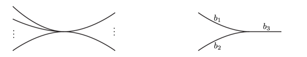
Figure 1. Switches. Left: a general switch. Right: a trivalent switch, with incident half-branches $b_{1}$, $b_{2}$, and $b_{3}$. The half-branches $b_{1}$ and $b_{2}$ are small and $b_{3}$ is large. The switch condition for a measure $\mu$ is that $\mu(b_{3})=\mu(b_{1})+\mu(b_{2})$.

Given a branch $b$ and some point $p$ in the interior of $b$, the components of $\mathrm{int}(b)\setminus p$ are called half-branches of $b$. Moreover, two half-branches of $b$ are equivalent if their intersection is a half-branch as well. Whenever we talk about half-branches, we mean an equivalence class of half-branches. Every switch is in the closure of three half-branches, two small half-branches bounding the cusp region and one large half-branch on the other side. Every branch contains two half-branches, and is called large if both of its half-branches are large.

We require train tracks to be filling, i.e., every connected component of $\Sigma\setminus\tau$ is either a polygon or a or once-punctured polygon. For every connected component $A$ of $\Sigma\setminus\tau$, an edge of $A$ is a maximal smooth arc $e\subset\tau\cap\partial A$.

Given train tracks $\tau$ and $\tau^{\prime}$ on $\Sigma$, we say $\tau$ carries $\tau^{\prime}$, and write $\tau^{\prime}<\tau$, if there exists a smooth map $f\nobreak\mskip 2.0mu\mathpunct{}\nonscript\mkern-3.0mu{:}\penalty 300\mskip 6.0mu plus 1.0mu\Sigma\to\Sigma$ homotopic to the identity such that $f(\tau^{\prime})\subset\tau$ and the restriction of $f$ to the tangent spaces of $\tau^{\prime}$ is non-singular. (This condition does not imply that $f$ sends switches to switches.) Similarly, we say a simple closed curve $\gamma$ is carried by a train track $\tau$, and write $\gamma<\tau$, if $\gamma$ is smoothly homotopic to a curve in $\tau$ via a map whose restriction to the tangent space of $\gamma$ is non-singular.

Roughly, the incidence matrix $M=\left(m_{ij}\right)$ for the carrying $\tau^{\prime}<\tau$ using the map $f$ is defined so that $m_{ij}$ is the number of times $f(b_{j}^{\prime})$ traverses $b_{i}$ in either direction. Here, $b_{i}$ and $b_{j}^{\prime}$ denote the $i$-th and $j$-th branches of $\tau$ and $\tau^{\prime}$, respectively. More precisely, to define the incidence matrix we fix a regular value $p_{i}$ of $f$ in the interior of each $b_{i}$ and let $m_{ij}$ be the number of preimages of $p_{i}$ in $b_{j}^{\prime}$. (Since switches may not map to switches, the incidence matrix may depend on the choice of $p_{i}$.)

A measure on a train track $\tau$ is a function $\mu$ that assigns a weight $\mu(b)\geq 0$ to each branch $b$ of $\tau$ and satisfies the switch condition as illustrated in Figure 1 at every switch of $\tau$. The pair $(\tau,\mu)$ is called a measured train track. If $\tau^{\prime}<\tau$, every measure $\mu^{\prime}$ on $\tau^{\prime}$ will induce a measure on $\tau$ where

$$\mu(b_{i})=\sum_{j}m_{ij}\mu(b_{j}^{\prime}).$$

Two measured train tracks are called equivalent if one is obtained from the other by a finite sequence of isotopies and the following moves.

1. Split. $(\tau^{\prime},\mu^{\prime})$ is obtained from $(\tau,\mu)$ by splitting a large branch $b$ if it is obtained from $(\tau,\mu)$ as in Figure 2. In this case, we write $(\tau,\mu)\rightharpoonup_{b}(\tau^{\prime},\mu^{\prime})$.

2. Shift. $(\tau^{\prime},\mu^{\prime})$ is obtained from $(\tau,\mu)$ by a shift if it is obtained by sliding one switch past another as in Figure 3. Note that the weights are not important in a shift move, so we do not specify them in the figure.

3. Fold. This is the inverse of the split move.

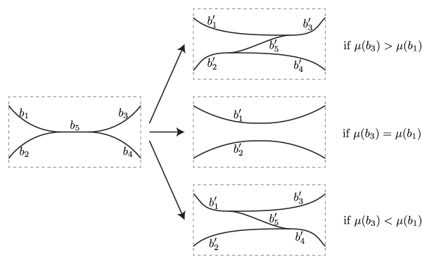
Figure 2. A split. There are three cases, depending on the relative weights of the branches.

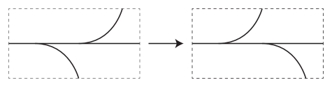
Figure 3. A shift. The weight of the inner edge is the sum of the weights of the two edges to its right; the other weights are unchanged by the move.

If $\tau^{\prime}$ is obtained from $\tau$ by a split or a shift then $\tau^{\prime}$ is carried by $\tau$. In the case of a split, the carrying map can be chosen to send switches to switches.

Following Penner-Harer [PH92, Section 1.7], a measured lamination on $\Sigma$ is a measured foliation of a closed subset of $\Sigma$. (There is a related concept of a measured geodesic lamination, which we will not explicitly use.) The space of measured laminations on $\Sigma$ is denoted by $\mathcal{ML}(\Sigma)$. Positive real numbers $\mathbb{R}_{+}$ act on $\mathcal{ML}(\Sigma)$ by multiplication and the quotient of $\mathcal{ML}(\Sigma)\setminus\{0\}$ by this action is called the space of projective measured laminations on $\Sigma$ and is denoted by $\mathcal{PML}(\Sigma)$. Here, $0$ denotes the empty lamination. Every measured train track $(\tau,\mu)$ specifies a well-defined measured lamination on $\Sigma$, and if two positively measured train tracks are equivalent then their corresponding measured laminations are isotopic [PH92, Theorem 2.7.4]. Conversely, if the corresponding measured laminations are isotopic, the measured train tracks are equivalent [PH92, Theorem 2.8.5]. That is, there is a bijection between the equivalence classes of measured train tracks and measured laminations. We say a measured lamination $(L,\mu_{0})$ on $\Sigma$ is suited to the train track $\tau$ if there exists a measure $\mu>0$ on $\tau$ such that $(L,\mu_{0})$ is isotopic to the measured lamination specified by $(\tau,\mu)$. If $(\tau^{\prime},\mu^{\prime})$ is obtained from $(\tau,\mu)$ by a shift or a split move, then $\tau^{\prime}$ is carried by $\tau$. So, measured laminations suited to $\tau^{\prime}$ are suited to $\tau$ as well.

A train track is called recurrent if it supports a positive measure (i.e., a measure satisfying $\mu(b)>0$ for every branch $b$).

A train track $\tau$ is called maximal if it is not a proper subtrack of another train track. A diagonal for $\tau$ is a smooth arc in one of the complementary regions of $\tau$ whose endpoints terminate tangentially at cusps and such that the union of $\tau$ with this arc is a train track. A train track $\tau^{\prime}$ is called a diagonal extension of $\tau$ if it is obtained from $\tau$ by adding pairwise disjoint diagonals. Note that if a train track $\tau$ is not maximal, one can construct a maximal diagonal extension $\tau^{\prime}$ of $\tau$, by adding diagonals. This maximal diagonal extension $\tau^{\prime}$ is not unique (and diagonal extensions are not generic train tracks).

Lemma 2.1.

Let $\tau$ be a train track suited to the unstable foliation of $\psi$ and let $\gamma\subset\Sigma$ be a simple closed curve. Then there is an integer $N$, such that for all $n>N$, $\psi^{n}(\gamma)$ is carried by some maximal diagonal extension of $\tau$ (possibly depending on $n$).

Proof.

By [FLP79, Corollary 12.3], as $n$ goes to infinity, $\psi^{n}(\gamma)$ converges to $[\mathcal{F}^{u},\mu_{u}]$, the image of the unstable foliation in the space of projective measured laminations $\mathcal{PML}(\Sigma)$. By [PH92, Proposition 1.4.9], there exists a maximal birecurrent (in the sense of [PH92, Section 1.3]) train track $\tau_{c}$ with $\tau<\tau_{c}$ and such that $\tau_{c}$ is obtained from $\tau$ by a sequence of trivial collapses along admissible arcs, as in [PH92, Figure 1.4.14]. By [PH92, Lemma 2.1.2], the measured laminations corresponding to the measures on $\tau_{c}$ form a polyhedron $U(\tau_{c})$. By [PH92, Lemma 3.1.2], the interior of $U(\tau_{c})$ is an open neighborhood of $[\mathcal{F}^{u},\mu_{u}]$ in $\mathcal{PML}(\Sigma)$. So, there exists an integer $N>0$ such that $\psi^{n}(\gamma)$ is in $U(\tau_{c})$ for all $n>N$.

On the other hand, for any maximal diagonal extension $\tau^{\prime}$ of $\tau$, the measured laminations corresponding to the measures on $\tau^{\prime}$ will form a polyhedron $U(\tau^{\prime})$ in $\mathcal{PML}(\Sigma)$, as well (see [PH92, Theorem 1.3.6, Lemma 2.1.2]). Moreover, [PH92, Proposition 2.2.2] implies that $U(\tau_{c})=\bigcup_{\tau^{\prime}}U(\tau^{\prime})$ where the union is over all maximal diagonal extensions $\tau^{\prime}$ of $\tau$. Therefore, for all $n>N$, $\psi^{n}(\gamma)$ is carried by some maximal diagonal extension $\tau^{\prime}$ of $\tau$ (not necessarily independent of $n$). ∎

A square matrix $M$ is called Perron-Frobenius if it has non-negative entries, and there exists an $n>0$ such that $M^{n}$ has strictly positive entries. It is a classical theorem that any Perron-Frobenius matrix $M$ has a positive, simple eigenvalue $\lambda$, the dominant eigenvalue, such that $\lambda>|r|$ for any other eigenvalue $r$ of $M$. Moreover, $M$ has an eigenvector with eigenvalue $\lambda$ whose entries are strictly positive. (See for instance [Gan59].)

By [PP87, Theorem 4.1] for any pseudo-Anosov diffeomorphism $\psi$, there exists a filling, generic train track $\tau$ such that $\psi(\tau)<\tau$ and the carrying map can be chosen such that the corresponding incidence matrix is Perron-Frobenius. The dominant eigenvector of the incidence matrix induces a positive measure on $\tau$, and this measured train track specifies the unstable foliation of $\psi$.

For a measured train track $(\tau,\mu)$ a maximal split is splitting $\tau$ simultaneously along all the large branches with maximum measure. If $(\tau^{\prime},\mu^{\prime})$ is obtained from $(\tau,\mu)$ by a maximal split, we write $(\tau,\mu)\rightharpoonup(\tau^{\prime},\mu^{\prime})$.

Theorem 2.2.

[Ago10, Theorem 3.5] Let $\psi$ be a pseudo-Anosov diffeomorphism of $\Sigma$ and $(\tau,\mu)$ be a measured train track suited to the unstable measured foliation $(\mathcal{F}^{u},\mu_{u})$ of $\psi$. Then there exist positive integers $n$ and $m$ such that

$$(\tau,\mu)\rightharpoonup(\tau_{1},\mu_{1})\rightharpoonup(\tau_{2},\mu_{2})\rightharpoonup\cdots\rightharpoonup(\tau_{n},\mu_{n})\rightharpoonup\cdots\rightharpoonup(\tau_{n+m},\mu_{n+m})$$

and $\tau_{n+m}=\psi(\tau_{n})$ and $\mu_{n+m}=\lambda(\psi)^{-1}\psi(\mu_{n})$.

A periodic splitting sequence for a pseudo-Anosov diffeomorphism $\psi$ is a sequence of train tracks suited to the unstable foliation formed by maximal splittings

$$(\tau_{n},\mu_{n})\rightharpoonup(\tau_{n+1},\mu_{n+1})\rightharpoonup\cdots\rightharpoonup(\tau_{n+m},\mu_{n+m})$$

such that $\tau_{n+m}=\psi(\tau_{n})$ and $\mu_{n+m}=\lambda(\psi)^{-1}\psi(\mu_{n})$. A periodic splitting sequence for $\psi$ is unique up to applying powers of $\psi$ and cyclic permutations (changing where in the loop one starts), so we will often abuse terminology and refer to the periodic splitting sequence for $\psi$.

Suppose $(\tau,\mu)$ is a train track from the periodic splitting sequence of some pseudo-Anosov diffeomorphism $\psi$. Then $\psi(\tau)<\tau$ with a carrying map induced by the sequence of maximal splits. The proof of [PP87, Theorem 4.1] implies that the incidence matrix for this carrying is Perron-Frobenius.

Lemma 2.3.

Let $\tau$ be a train track from the periodic splitting sequence for $\psi$. For any maximal diagonal extension $\widetilde{\tau}$ of $\tau$, there exists a carrying of $\psi(\widetilde{\tau})$ by some (possibly distinct) maximal diagonal extension $\widetilde{\tau}^{\prime}$ of $\tau$ such that the restriction of this carrying map to the subtrack $\psi(\tau)\subset\psi(\widetilde{\tau})$ coincides with the carrying map $\psi(\tau)<\tau$.

Proof.

The train track $\tau$ is filling, so every connected component of $\Sigma\setminus\tau$ is a polygon or once-punctured polygon. Let $B$ be one of these complementary regions and suppose $B$ is an $n$-gon, so the boundary of $B$ contains $n$ cusps. Denote the corresponding switches by $s_{1},s_{2},\dots,s_{n}$, indexed counterclockwise. Denote the $n$ train paths that give the edges of $B$ by $\rho_{1},\rho_{2},\dots,\rho_{n}$, where $\rho_{i}$ connects $s_{i}$ to $s_{i+1}$ for all $i$ (and $s_{n+1}\coloneqq s_{1}$).

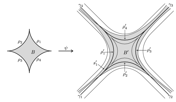
Figure 4. The image of a 4-gon $B$ under $\psi$. Thick lines indicate the train track $\tau$. Thin lines indicate the boundary of a fibered neighborhood of $\tau$. The shaded region is $B$ (left) and the image of $B$ (right). The image of $B$ and the train paths $\gamma_{i}$ extend beyond the picture. (In the drawing, near the singular point $\psi$ sends $B$ by a $135^{\circ}$ twist.)

The diffeomorphism $\psi$ maps each singular point of the unstable foliation (respectively puncture of $\Sigma$) to a singular point (respectively puncture). Moreover, since $\psi(\tau)$ is obtained from $\tau$ by a sequence of splits, we may assume the carrying map $\psi(\tau)<\tau$ sends switches to switches. Each connected component $B$ of $\Sigma\setminus\tau$ contains either one singular point or one puncture. If $B$ contains a singular point (respectively puncture), then $\psi(B)$ will contain a singular point (respectively puncture). Denote the component of $\Sigma\setminus\tau$ containing the image of that point under $\psi$ by $B^{\prime}$. Note that $B^{\prime}$ is also an $n$-gon and might coincide with $B$. The boundary of $B^{\prime}$ is a union of $n$ train paths $\rho_{1}^{\prime},\rho_{2}^{\prime},\dots,\rho_{n}^{\prime}$, indexed counterclockwise. Denote the switches corresponding to the cusps on the boundary of $B^{\prime}$ by $s_{1}^{\prime},s_{2}^{\prime},\dots,s_{n}^{\prime}$ such that $\rho_{i}^{\prime}$ connects $s_{i}^{\prime}$ to $s_{i+1}^{\prime}$ (and $s_{n+1}^{\prime}\coloneqq s_{1}^{\prime}$). Then there exist train paths $\gamma_{1},\gamma_{2},\dots,\gamma_{n}$ such that $\gamma_{i}$ ends in the large branch of $s_{i}^{\prime}$ and the image of $\psi(\rho_{i})$ under the carrying map is equal to $\gamma_{i+k}\circ\rho_{i+k}^{\prime}\circ\gamma_{i+k+1}^{-1}$, where indices are taken modulo $n$. Here, $0\leq k\leq n-1$ is a constant, depending on the singular point in $B$. See Figure 4.

With this description in hand, we are ready to describe $\widetilde{\tau}^{\prime}$. For each diagonal $d$ in $B$ of $\widetilde{\tau}$ that connects $s_{i}$ to $s_{j}$ we add the diagonal $d^{\prime}$ in $B^{\prime}$ that connected $s_{i}^{\prime}$ to $s_{j}^{\prime}$. These new diagonals give the maximal diagonal extension $\widetilde{\tau}^{\prime}$. It is straightforward that the carrying map $\psi(\tau)<\tau$ extends to a carrying map $\psi(\widetilde{\tau})<\widetilde{\tau}^{\prime}$. For instance, under this extension a diagonal $d$ in $B$ connecting $s_{i}$ to $s_{j}$ is mapped to $\gamma_{i}^{-1}d^{\prime}\gamma_{j}$. ∎

Associated to any filling train track $\tau$ on $\Sigma$, there is a dual triangulation $\mathcal{T}$ of $\Sigma$, defined so that the dual edge has one vertex in every component of $\Sigma\setminus\tau$ and one edge dual to every branch of $\tau$ such that it intersects the branch transversely and connects the vertices in the components of $\Sigma\setminus\tau$ adjacent to the branch. Moreover, if a component of $\Sigma\setminus\tau$ is punctured then the vertex in that component coincides with the puncture. If $\tau^{\prime}$ is obtained from $\tau$ by a split, its dual triangulation $\mathcal{T}^{\prime}$ is obtained from $\mathcal{T}$ by a Whitehead move as depicted in Figure 5.

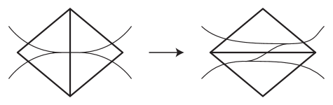
Figure 5. A Whitehead move. The train track is drawn in a thin line, and the dual triangulation in a thick line. When the train track changes by a split, the dual triangulation changes by a Whitehead move.

A bigon track is a branched $1$-dimensional submanifold of $\Sigma$ that fails to be a train track because some of its complementary regions are bigons. A bigon track is called generic if all of its switches are trivalent.

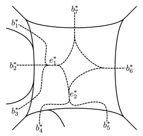
Figure 6. Dual bigon track. A piece of a train track is shown (solid) together the corresponding piece of its dual bigon track (dashed).

Given a train track $\tau$, the dual bigon track $\tau^{*}$ is defined as follows. For each branch $b_{i}$ of $\tau$ consider a small arc $b_{i}^{*}$ transversely intersecting $b_{i}$ at one point and disjoint from every $b_{j}$ with $j\neq i$. Moreover, arrange that the arcs $b_{1}^{*},b_{2}^{*},\dots,b_{l}^{*}$ are pairwise disjoint. Let $A$ be a connected component of $\Sigma\setminus\tau$. For each edge $e$ of $A$, join the dual arcs to the branches contained in $e$ by a switch in $A$ with the dual arcs on one side and a new branch $e^{*}$ on the other side. So, for example, if $e=\overline{b_{i_{1}}}\cup\overline{b_{i_{2}}}\cup\cdots\cup\overline{b_{i_{k}}}$, the arcs $b_{i_{1}}^{*},b_{i_{2}}^{*},\dots,b_{i_{k}}^{*}$ will merge together and form a switch of valence $k+1$. For any cusp singularity in $\partial A$ with adjacent edges $e_{1}$ and $e_{2}$, connect the new branches $e_{1}^{*}$ and $e_{2}^{*}$ with a new smooth branch, as in Figure 6. Note that these branches are chosen such that for each switch of $\tau$ there is a bigon region in $\Sigma\setminus\tau^{*}$ that contains the switch. Therefore, if $A$ is a once-punctured $n$-gon the corresponding $n$-gon component of $\Sigma\setminus\tau^{*}$ inside $A$ is once-punctured as well. Note that $\tau^{*}$ is not necessarily generic. Moreover, $\tau^{*}$ and $\tau$ intersect efficiently i.e. there is no embedded bigon on $\Sigma$ whose boundary is the union of a smooth arc on $\tau$ and a smooth arc on $\tau^{*}$. See [PH92, Section 3.4] for more detailed discussion of dual bigon tracks.

Lemma 2.4.

Let $\tau$ be a train track suited to the unstable foliation of $\psi$ and let $\gamma\subset\Sigma$ be a simple closed curve. Then there is an integer $N$ such that for all $n>N$, $\psi^{-n}(\gamma)$ is carried by some maximal diagonal extension of the dual bigon track $\tau^{*}$ (possibly depending on $n$).

Proof.

By [FLP79, Corollary 12.3], as $n$ goes to infinity, $\psi^{-n}(\gamma)$ converges to $[\mathcal{F}^{s},\mu_{s}]$, the image of the stable foliation in the space of projective measured laminations $\mathcal{PML}(\Sigma)$. By [PH92, Proposition 1.4.9] one can obtain a maximal birecurrent train track ${\tau}_{c}$ from $\tau$ by a sequence of trivial collapses along admissible arcs. Then, a corresponding sequence of split moves on ${\tau}_{c}$ will result in a generic maximal and birecurrent train track $\tau^{\prime}$ such that $\tau^{\prime}$ is the result of combing a maximal diagonal extension of $\tau$ [PH92, Figure 1.4.2].

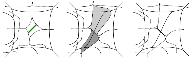
Figure 7. Collapsing admissible arcs. Left: the train track $\tau$ (solid), its dual bigon track $\tau^{*}$ (dashed), and an admissible arc (thick). Center: the train track $\tau^{\prime}$ obtained from adding a diagonal to $\tau$ and combing it to make the result generic, its dual bigon track $(\tau^{\prime})^{*}$. Right: the (dashed) bigon track $\tau^{*}_{c}$ obtained by collapsing the two shaded bigons, which coincides with the bigon track obtained from $\tau^{*}$ by a trivial collapse along the admissible thick arc in left figure.

The dual bigon track $(\tau^{\prime})^{*}$ is birecurrent and maximal [PH92, Proposition 3.4.5]. Collapsing the bigons corresponding to the endpoint switches of the added diagonals results in a bigon track $\tau^{*}_{c}$, which can also be obtained from $\tau^{*}$ by trivial collapses along admissible arcs (see Figure 7). Note that the measured laminations corresponding to the measures on $(\tau^{\prime})^{*}$ and $\tau^{*}_{c}$ are the same. There is a positive measure $\mu^{*}$ on $\tau^{*}$ such that $(\tau^{*},\mu^{*})$ is suited to $[\mathcal{F}^{s},\mu_{s}]$ [PH92, Epilogue]. Since $\tau^{*}<\tau^{*}_{c}$, the positive measure $\mu^{*}$ induces a positive measure $\mu^{*}_{c}$ on $\tau^{*}_{c}$ so that $(\tau^{*}_{c},\mu^{*}_{c})$ is suited to $[\mathcal{F}^{s},\mu_{s}]$. Therefore, the measured laminations corresponding to the measures on $\tau^{*}_{c}$ form a polytope whose interior is an open neighborhood of $[\mathcal{F}^{s},\mu_{s}]$ [PH92, Proposition 3.4.1]. Then, as in the proof of Lemma 2.1, by [PH92, Proposition 2.2.2] this neighborhood is the union of measured laminations corresponding to the maximal diagonal extensions of $\tau^{*}$. Therefore, there exists an $N>0$ such that for all $n>N$, $\psi^{-n}(\gamma)$ is carried by some maximal diagonal extension of $\tau^{*}$ (not necessarily independent of $n$). ∎

3. Spheres and compression bodies

In this section, we prove four elementary lemmas about decompositions of 3-manifolds, handlebodies, and compression bodies, needed for the detection results later. The first is a specific version of the prime factorization, in terms of the Hurewicz homomorphism. The second lemma uses the first to give a simple criterion for a 3-manifold to be a handlebody. The third is a criterion for a collection of disks to generate a compression body. The last is a generalization of a result of Haken’s about how spheres intersect Heegaard surfaces to the case of compression body splittings.

Lemma 3.1.

Let $Y$ be a compact, connected, oriented $3$-manifold. Suppose that the image of the Hurewicz homomorphism $\pi_{2}(Y)\to H_{2}(Y)$ generates an $n$-dimensional subspace of $H_{2}(Y;\mathbb{Q})$. Then there is an integer $0\leq k\leq n$, a closed 3-manifold $Y^{\prime}$, and 3-manifolds $Y_{1},\dots,Y_{n-k+1}$ with non-empty boundary so that

$$Y=\begin{cases}Y^{\prime}\#\overbrace{(S^{2}\times S^{1})\#\cdots\#(S^{2}\times S^{1})}^{k}\#Y_{1}\#\cdots\#Y_{n-k+1}&\text{if }\partial Y\neq\emptyset\\ Y^{\prime}\#\overbrace{(S^{2}\times S^{1})\#\cdots\#(S^{2}\times S^{1})}^{n}&\text{if }\partial Y=\emptyset.\end{cases}$$

Further, $Y^{\prime}$ and every $Y_{i}$ does not contain any homologically essential $2$-spheres.

Proof.

Choose a prime decomposition

(3.2) $$Y=Y^{\prime}_{1}\#\cdots\#Y^{\prime}_{j}\#\overbrace{(S^{2}\times S^{1})\#\cdots\#(S^{2}\times S^{1})}^{k}\#Y_{1}\#\cdots\#Y_{\ell}$$

of $Y$, where each $Y_{i}$ and $Y^{\prime}_{i}$ is irreducible (every sphere bounds a ball or equivalently, by the Sphere Theorem, each $Y_{i}$ and $Y^{\prime}_{i}$ has trivial $\pi_{2}$), each $Y_{i}$ has nonempty boundary, and each $Y^{\prime}_{i}$ is closed. If $S$ is a sphere in $Y$ then, intersecting $S$ with the connect sum spheres in Formula (3.2) and using an innermost disk argument, $[S]\in H_{2}(Y)$ is a linear combination of spheres in the $Y^{\prime}_{i}\setminus B^{3}$, the copies of $(S^{2}\times S^{1})\setminus B^{3}$, and the $Y_{i}\setminus B^{3}$. Since $Y^{\prime}_{i}$ is closed, from the diagram

the image of the Hurewicz map to $H_{2}(Y_{i}^{\prime}\setminus B^{3})$ vanishes. Similarly, the image of the Hurewicz map to $(S^{2}\setminus S^{1})\setminus B^{3}$ is generated by $[S^{2}\times\{pt\}]$, and for $Y_{i}\setminus B^{3}$, the analogous diagram

the image of the Hurewicz map to $H_{2}(Y^{\prime}_{i}\setminus B^{3})$ is generated by the boundary sphere. So, $[S]$ is a linear combination of the spheres $[S^{2}\times\{pt\}]$ for the $S^{2}\times S^{1}$ factors and the boundary spheres for the $Y_{i}$ factors. Further, the sum of all the boundary spheres vanishes in $H_{2}(Y)$. So, $k+\ell=n+1$, and letting $Y^{\prime}=Y^{\prime}_{1}\#\cdots\#Y^{\prime}_{j}$ gives the desired factorization.

The proof for the closed case is the same, except that $\ell=0$ and $k=n$. ∎

A homology handlebody of genus $g$ is a compact, connected, orientable $3$-manifold $Y$ with boundary a connected surface of genus $g$ so that the map $H_{1}(\partial Y)\to H_{1}(Y)$ is surjective. (We will generally assume that $g>0$. Also, $H_{1}(\partial Y)\to H_{1}(Y)$ being surjective implies that $H_{1}(Y,\partial Y)=0$ so, since the torsion subgroup of $H_{1}(Y)=H^{2}(Y,\partial Y)$ is $\operatorname{Ext}^{1}(H_{1}(Y,\partial Y),\mathbb{Z})$, this implies that $H_{1}(Y)$ is free.)

We can use Lemma 3.1 to give a criterion for recognizing handlebodies among homology handlebodies, which is key to the proof of Theorem 1.1:

Lemma 3.3.

Let $Y$ be an irreducible homology handlebody of genus $g$. Then $Y$ is a handlebody of genus $g$ if and only if the homology $H_{2}(D(Y);\mathbb{Q})$ of the double $D(Y)=Y\cup_{\partial}(-Y)$ is generated by $2$-spheres.

Proof.

If $Y$ is a handlebody then certainly $H_{2}(D(Y))$ is generated by $2$-spheres. For the converse, suppose $H_{2}(D(Y);\mathbb{Q})$ is generated by $2$-spheres. By Lemma 3.1, $H_{2}(D(Y);\mathbb{Q})$ is generated by disjoint, embedded $2$-spheres. We first reduce to the case that $Y$ is not a boundary sum of two manifolds. If $Y=Y_{1}\#_{b}Y_{2}$ then $D(Y)=D(Y_{1})\#D(Y_{2})$. It follows from the proof of Lemma 3.1 that both $H_{2}(D(Y_{1});\mathbb{Q})$ and $H_{2}(D(Y_{2});\mathbb{Q})$ are generated by $2$-spheres. Moreover, if $Y_{1}$ and $Y_{2}$ are handlebodies, then $Y$ is also a handlebody.

So, assume that $Y$ is not a boundary sum. Let $\Sigma=\partial Y$. Consider an embedded $2$-sphere $S$ in $DY$ that is a generator of $H_{2}(D(Y);\mathbb{Q})$. It follows from the irreducibility of $Y$ that $S$ intersects $\Sigma$. Further, we may arrange for $S$ to intersect $\Sigma$ minimally, i.e., that none of the disks in $S\cap Y$ or $S\cap-Y$ are homotopic relative boundary to disks in $\Sigma$. Choose a disk $D$ in $S\cap Y$ or $S\cap-Y$. Since $Y$ is not a boundary sum, $D$ is homologically essential. Since $Y$ is a homology handlebody, the map $H^{1}(Y)\to H^{1}(\partial Y)$ is injective, so there is a circle in $\partial Y$ intersecting $\partial D$ in a single point. This gives a decomposition of $Y$ as the boundary sum of a solid torus with a $3$-manifold $Y^{\prime}$. Hence, $Y^{\prime}$ is a $3$-ball and $Y$ is a solid torus. ∎

Before giving the next two results, we introduce some terminology related to compression bodies. Let $\Sigma$ be a closed, orientable surface of genus $g$. Given disjoint curves $\gamma_{1},\dots,\gamma_{n}\subset\Sigma$ there is an associated 3-manifold $\Sigma[\gamma_{1},\dots,\gamma_{n}]$ obtained from $[0,1]\times\Sigma$ by attaching 2-handles along the $\gamma_{i}\times\{1\}$ and filling any $S^{2}$ boundary components of the result with 3-balls. A compression body $C$ is a manifold homeomorphic to some $\Sigma[\gamma_{1},\dots,\gamma_{n}]$. We refer to (the image of) the boundary component $\{1\}\times\Sigma$ of the result as the outer boundary $\partial_{\mathit{out}}C$ and the remaining boundary components as the inner boundary $\partial_{\mathit{in}}C$. Since we do not require the attaching circles for the 2-handles to be homologically linearly independent, the inner boundary may not be connected. A handlebody is the special case that the inner boundary is empty. A basis for $C$ is a set of pairwise disjoint simple closed curves $\{\gamma_{1},\cdots,\gamma_{n}\}$ on $\partial_{\mathit{out}}C$ so that $C\cong(\partial_{\mathit{out}}C)[\gamma_{1},\cdots,\gamma_{n}]$.

Since we are interested in bordered Floer theory, we will be interested in compression bodies whose boundaries are parameterized by surfaces associated to pointed matched circles or arc diagrams. Define a half-bordered compression body to be a compression body $C$ together with a diffeomorphism $\phi$ from a reference surface $\Sigma$ to $\partial_{\mathit{out}}C$. An essential simple closed curve $\gamma\subset\Sigma$ is a meridian for $C$ if $\phi(\gamma)$ bounds a disk in $C$.

A compression body splitting of a 3-manifold $Y$ is a decomposition $Y=C\cup_{\Sigma}C^{\prime}$ as a union of two compression bodies glued along their outer boundaries $\Sigma$.

The following lemma gives a criterion for when a set of meridians for a compression body is large enough to determine the compression body; this will be used in detecting when diffeomorphisms extend over specific compression bodies.

Lemma 3.4.

Let $(C,\phi\nobreak\mskip 2.0mu\mathpunct{}\nonscript\mkern-3.0mu{:}\penalty 300\mskip 6.0mu plus 1.0mu\Sigma\to\partial_{\mathit{out}}C)$ be a half-bordered compression body. Let $\amalg_{i=1}^{n}\gamma_{i}\subset\Sigma$ be a collection of pairwise disjoint meridians for $C$ and consider pairwise disjoint, properly embedded disks $\amalg_{i=1}^{n}D_{i}\subset C$ such that $\partial D_{i}=\phi(\gamma_{i})$ for all $i$. Then $\Sigma[\gamma_{1},\gamma_{2},\dots,\gamma_{n}]\cong C$ if and only if the homology classes $[D_{1}],[D_{2}],\dots,[D_{n}]$ generate $H_{2}(C,\partial_{\mathit{out}}(C))$.

Proof.

First, it is easy to see that the homology classes of the cores of the attached $2$-handles in $\Sigma[\gamma_{1},\gamma_{2},\dots,\gamma_{n}]$ generate $H_{2}(\Sigma[\gamma_{1},\gamma_{2},\dots,\gamma_{n}],\Sigma)$, and so if $\Sigma[\gamma_{1},\gamma_{2},\dots,\gamma_{n}]\cong C$ then $[D_{1}],[D_{2}],\dots,[D_{n}]$ generate $H_{2}(C,\partial_{\mathit{out}}(C))$.

On the other hand, suppose $[D_{1}],[D_{2}],\dots,[D_{n}]$ generate $H_{2}(C,\partial_{\mathit{out}}(C))$. If we show that $\amalg_{i=1}^{n}\gamma_{i}$ is a maximal set of meridians for $C$, then the claim follows from [BV17, Lemma 2.1] (which states that attaching 2-handles along any maximal set of meridians for a compression body $C$ gives $C$). Let $\gamma\subset\Sigma$ be a simple closed curve disjoint from $\amalg_{i=1}^{n}\gamma_{i}$ such that $\phi(\gamma)=\partial D$ for a properly embedded disk $D$ in $C$. The homology class $[D]\in H_{2}(C,\partial_{\mathit{out}}(C))$ is equal to a linear combination of $[D_{1}],[D_{2}],\dots,[D_{n}]$ and so $\mathrm{nbd}(\partial_{\mathit{out}}(C))\cup(\amalg_{i=1}^{n}\mathrm{nbd}(D_{i}))\cup\mathrm{nbd}(D)$ has an $S^{2}$ boundary component that intersects $\mathrm{nbd}(D)$ nontrivially. Consequently, $\gamma$ is homotopic to a homotopically trivial curve in the inner boundary of $\Sigma[\gamma_{1},\gamma_{2},\cdots,\gamma_{n}]$ and so $\amalg_{i=1}^{n}\gamma_{i}$ is maximal. ∎

The following result shows that prime decompositions can be chosen to be compatible with compression body splittings. The case of Heegaard splittings (handlebodies) is due to Haken [Hak68] (but we learned it from Ghiggini-Lisca [GL15, Lemma 3.4]):

Lemma 3.5.

Let $Y=C\cup_{\Sigma}C^{\prime}$ be a compression body splitting of a $3$-manifold $Y$ with prime factorization of the form

$$Y=Y_{1}\#\cdots\#Y_{k}\#(S^{2}\times S^{1})^{l}\#Y^{\prime}_{1}\#\cdots\#Y^{\prime}_{h},$$

where each $Y_{i}$ has nonempty boundary and every $Y^{\prime}_{j}$ is closed. Moreover, assume that $\operatorname{rank}(H_{2}(Y)/i_{*}(H_{2}(\partial Y)))=l$, where $i$ denotes the inclusion map. Then there exist pairwise disjoint, embedded $2$-spheres $S_{1},\dots,S_{k+l-1}$ in $Y$ satisfying the following conditions:

1. Each $S_{i}$ intersects the surface $\Sigma$ in a single circle $C_{i}$.

2. The homology classes $[S_{1}],[S_{2}],\dots,[S_{k+l-1}]$ are linearly independent in $H_{2}(Y)$.

3. The homology classes $[S_{1}],[S_{2}],\dots,[S_{l}]$ span $H_{2}(Y;\mathbb{Q})/i_{*}(H_{2}(\partial Y;\mathbb{Q}))$.

(In the case that $Y$ is closed, Condition (2) is redundant.)

Proof.

The prime factorization of $Y$ implies that for $n=k+l-1$ there exist embedded $2$-spheres $S_{1},S_{2},\dots,S_{n}$ in $Y$ such that conditions (2) and (3) hold for them. Following an analogous argument of Haken’s [Hak68, pp. 84–86], we show that one can construct a collection of pairwise disjoint, essential embedded $2$-spheres $S^{\prime}_{1},S^{\prime}_{2},\dots,S^{\prime}_{n^{\prime}}$ so that $n^{\prime}\geq n$, each $S^{\prime}_{i}$ intersects $\Sigma$ in a single circle and the subspace of $H_{2}(Y)$ generated by the homology classes $[S^{\prime}_{1}],\dots,[S^{\prime}_{n^{\prime}}]$ contains the subspace generated by $[S_{1}],[S_{2}],\dots,[S_{n}]$. As a result, we can find $\{j_{1},\dots,j_{n}\}\subset\{1,2,\dots,n^{\prime}\}$ such that the homology classes $[S^{\prime}_{j_{1}}],[S_{j_{2}}^{\prime}],\dots,[S^{\prime}_{j_{l}}]$ span $H_{2}(Y;\mathbb{Q})/i_{*}(H_{2}(\partial Y;\mathbb{Q}))$ and $[S^{\prime}_{j_{1}}],[S^{\prime}_{j_{2}}],\dots,[S^{\prime}_{j_{n}}]$ are linearly independent in $H_{2}(Y)$, and we are done.

Step 1. We show that the spheres can be changed via isotopy so that every connected component of $S_{i}\cap C^{\prime}$ is a disk representing a nontrivial homology class in $H_{2}(C^{\prime},\partial_{\mathit{out}}C^{\prime})$ for all $1\leq i\leq n$. If $\partial_{\mathit{in}}C^{\prime}=\emptyset$, then $C^{\prime}$ is a handlebody and this is Step $1$ of Haken’s proof. Suppose $\partial_{\mathit{in}}C^{\prime}\neq\emptyset$. Consider pairwise disjoint, properly embedded arcs $\gamma_{1},\dots,\gamma_{m}$ in $C^{\prime}$ so that $\partial\gamma_{i}\subset\partial_{\mathit{in}}C^{\prime}$ for all $i$ and the homology classes $[\gamma_{1}],\dots,[\gamma_{m}]$ form a basis for $H_{1}(C^{\prime},\partial_{\mathit{in}}C^{\prime})$. Moreover, assume $S_{i}$ and $\gamma_{j}$ intersect transversely for all $i,j$. Let $C^{\prime\prime}\subset C^{\prime}$ be the compression body defined as a small neighborhood of $\partial_{\mathit{in}}C^{\prime}\cup\gamma_{1}\cup\cdots\cup\gamma_{m}$, so that every component of $S_{i}\cap C^{\prime\prime}$ is a disk, for all $i$. There is an ambient isotopy $h$ that maps $C^{\prime\prime}$ to $C^{\prime}$. Let $S_{1,i}=h(S_{i})$ for $1\leq i\leq n$.

Denote the number of connected components in $\left(\coprod_{i=1}^{n}S_{1,i}\right)\cap\Sigma$ by $c_{1}$.

Step 2. We transform the spheres $S_{1,1},\dots,S_{1,n}$ from Step 1 into a collection of pairwise disjoint embedded spheres $S_{2,1},\dots,S_{2,n^{\prime}}$ so that they still satisfy conditions (2) and (3), $\left(\coprod_{i=1}^{n}S_{2,i}\right)\cap C$ is incompressible in $C$ and

$$\left(\coprod_{i=1}^{n^{\prime}}S_{2,i}\right)\cap\Sigma\subset\left(\coprod_{i=1}^{n}S_{1,i}\right)\cap\Sigma.$$

If we define $c_{2}$ to be the number of connected components of $\left(\coprod_{i=1}^{n^{\prime}}S_{2,i}\right)\cap\Sigma$, the last condition is $c_{2}\leq c_{1}$.

If $\left(\coprod_{i=1}^{n}S_{1,i}\right)\cap C$ is incompressible in $C$, then let $n=n^{\prime}$ and $S_{2,i}=S_{1,i}$ for all $i$. So, suppose $\left(\coprod_{i=1}^{n}S_{1,i}\right)\cap C$ is not incompressible. Let $\gamma\subset(S_{1,i}\cap C)$ be a circle that bounds a compressing disk $D$ in $C$. By an innermost disk argument, we can assume that the interior of $D$ is disjoint from the spheres $S_{1,i}$. Remove a small tubular neighborhood $\mathrm{nbd}(\gamma)$ of $\gamma$ from $S_{1,i}$ and add two parallel copies of $D$ to $\partial\mathrm{nbd}(\gamma)$. Denote the resulting spheres by $S_{11,i}$ and $S_{12,i}$. If one of $S_{11,i}$ or $S_{12,i}$, say $S_{11,i}$, bounds a ball in $Y$, then replace $S_{1,i}$ with $S_{12,i}$. Otherwise, if both $S_{11,i}$ and $S_{12,i}$ are essential in $Y$, then replace $S_{1,i}$ with the two spheres $S_{11,i}$ and $S_{12,i}$. Repeat this process until the intersection of our spheres with $C$ is incompressible in $C$. Denote the resulting spheres by $S_{2,1},\dots,S_{2,n^{\prime}}$. It is obvious that

$$\left\langle[S_{1,1}],\dots,[S_{1,n}]\right\rangle\subset\left\langle[S_{2,1}],\dots,[S_{2,n^{\prime}}]\right\rangle.$$

Before going to the next step, we introduce some more notation. Let

$$a_{2}=c_{2}-\left|\left(\coprod_{i=1}^{n^{\prime}}S_{2,i}\right)\cap C\right|$$

and let $b_{2}$ be $a_{2}$ minus the number of non-disk components in $\left(\coprod_{i=1}^{n^{\prime}}S_{2,i}\right)\cap C$. Then $a_{2}\geq 0$, because otherwise one of the spheres $S_{2,i}$ is disjoint from $\Sigma$ and lies in $C$, which contradicts the incompressibility of $S_{2,i}$. So, if $a_{2}=0$, then all connected components of $S_{2,i}\cap C$ are disks, and we are done. If $a_{2}\neq 0$ then $a_{2}>b_{2}\geq 0$.

Step 3. Suppose $a_{2}>0$. We use an isotopy to transform $S_{2,1},\dots,S_{2,n^{\prime}}$ into $S_{3,1},\dots,S_{3,n^{\prime}}$ such that $c_{3}<c_{2}$ and $a_{3}=b_{3}=0$, where $a_{3},b_{3}$ and $c_{3}$ are defined similar to $a_{2},b_{2}$ and $c_{2}$. However, the connected components of $\left(\coprod_{i=1}^{n^{\prime}}S_{3,i}\right)\cap C^{\prime}$ might no longer be disks.

Consider a set of pairwise disjoint, properly embedded disks $D_{1},D_{2},\dots,D_{m}$ in $C$ such that $\partial D_{i}\subset\partial_{\mathit{out}}C$ and

$$\begin{cases}C\setminus\left(\coprod_{i=1}^{m}\mathrm{nbd}(D_{i})\right)\cong[0,1]\times\partial_{\mathit{in}}C&\text{if }\partial_{\mathit{in}}C\neq\emptyset\\ B^{3}&\text{if }\partial_{\mathit{in}}C=\emptyset.\end{cases}$$

Moreover, assume every $D_{i}$ intersects all the spheres $S_{2,j}$ transversely. So, $D_{i}\cap S_{2,j}$ is a collection of arcs and circles. First, every disk $D_{i}$ can be transformed via isotopies so that $D_{i}\cap\left(\coprod_{j=1}^{n^{\prime}}S_{2,j}\right)$ has no circle components, as follows. Consider an innermost circle component $\gamma$ on $D_{i}$, i.e., a circle $\gamma$ which bounds a disk $a$ in $D_{i}$ disjoint from $\coprod_{j=1}^{n^{\prime}}S_{2,j}$. Then the incompressibility of $C\cap\left(\coprod_{j=1}^{n^{\prime}}S_{2,j}\right)$ in $C$ implies that $\gamma$ bounds a disk $b$ in $\coprod_{j=1}^{n^{\prime}}S_{2,j}$. The union of $a$ and $b$ is an embedded $2$-sphere in $C$ and so bounds a $3$-ball. Pushing $D_{i}$ (and possibly other disks that have nonempty intersection with this $3$-ball) via an isotopy through this $3$-ball will remove the intersection circle $\gamma$. Repeat this process until every connected component of $D_{i}\cap S_{2,j}$ is an arc, for all $i$ and $j$.

Second, say that an arc $\gamma\subset D_{i}\cap S_{2,j}$ splits off a disk from $S_{2,j}\cap C$ if one of the components of $(S_{2,j}\cap C)\setminus\gamma$ is a disk $D$ with $\gamma$ on its boundary. We transform our collection of embedded disks $D_{1},\dots,D_{m}$ such that all the aforementioned properties hold, and none of the arc components in $D_{i}\cap S_{2,j}$ splits off a disk from $S_{2,j}\cap C$, for every $i$ and $j$. Consider an intersection arc $\gamma$ in $S_{2,j}\cap C$ that splits off a disk $D$ and which is innermost in the sense that the interior of $D$ is disjoint from $\coprod_{i=1}^{m}D_{i}$. Remove a small neighborhood $\mathrm{nbd}(\gamma)$ of $\gamma$ from $D_{i}$ and add two parallel copies of $D$ to $D_{i}\setminus\mathrm{nbd}(\gamma)$ to construct two properly embedded disks $D_{i}^{\prime}$ and $D_{i}^{\prime\prime}$ with boundary on $\partial_{\mathit{out}}(C)$ in $C$. After small isotopies we may assume $D_{i}$, $D_{i}^{\prime}$ and $D_{i}^{\prime\prime}$ are pairwise disjoint. Since $C\setminus\left(\coprod_{i=1}^{m}\mathrm{nbd}(D_{i})\right)$ is a product, the disks $D_{i}^{\prime}$ and $D_{i}^{\prime\prime}$ are boundary-parallel in $C\setminus\left(\coprod_{i=1}^{m}\mathrm{nbd}(D_{i})\right)$, so there is a $3$-ball $B_{i}^{\prime}$ (respectively $B_{i}^{\prime\prime}$) with part of its boundary $D_{i}^{\prime}$ (respectively $D_{i}^{\prime\prime}$) and the rest on the boundary of $C\setminus\left(\coprod_{i=1}^{m}\mathrm{nbd}(D_{i})\right)$. After an isotopy, we may assume that the $3$-balls $B_{i}^{\prime}$ and $B_{i}^{\prime\prime}$ are either disjoint or one is contained in the other; but if $B_{i}^{\prime}\cap B_{i}^{\prime\prime}=\emptyset$ then their union together with the region between $D_{i}$ and $D^{\prime}_{i}\cup D^{\prime\prime}_{i}$ is a $3$-ball, showing that $D_{i}$ is boundary parallel, a contradiction. So, without loss of generality, we may assume that $B_{i}^{\prime\prime}\supset B_{i}^{\prime}$. Then it is easy to check that replacing $D_{i}$ with $D_{i}^{\prime\prime}$ will result in a set of disks that still splits $C$ into a $3$-manifold homeomorphic to $[0,1]\times\partial_{\mathit{in}}C$ or into $B^{3}$. Repeat this process until none of the arc components in $D_{i}\cap S_{2,j}$ splits off a disk from $S_{2,j}\cap C$, for every $i$ and $j$.

Third, we remove the rest of the intersection arcs by isotoping $\coprod_{i=1}^{n^{\prime}}S_{2,i}$ as follows. Consider an innermost intersection arc $\gamma\subset D_{i}\cap\left(\coprod_{i=1}^{n^{\prime}}S_{2,i}\right)$ on $D_{i}$, in the sense that one of the two components in $D_{i}\setminus\gamma$, denoted by $D_{i}^{\prime}$, is disjoint from $\coprod_{i=1}^{n^{\prime}}S_{2,i}$. Suppose $\gamma\subset S_{2,j}$. Then transform $S_{2,j}$ by an isotopy that pushes $S_{2,j}$ along $D_{i}^{\prime}$ through $\Sigma$ and removes the intersection arc $\gamma$. Depending on $\gamma$ one of the following happens:

• If $\gamma$ connects distinct components of $\Sigma\cap\left(\coprod_{i=1}^{n^{\prime}}S_{2,j}\right)$, then $c_{2}$ and $a_{2}$ decrease by $1$, and $b_{2}$ does not increase.

• If $\partial\gamma$ lies on a single component of $\Sigma\cap\left(\coprod_{i=1}^{n^{\prime}}S_{2,j}\right)$, then $c_{2}$ increases by $1$, $a_{2}$ does not change, and $b_{2}$ decreases by $1$.

Repeat this process until we get a collection of embedded $2$-spheres $S_{2,1}^{\prime},S_{2,2}^{\prime},\dots,S_{2,n^{\prime}}^{\prime}$ disjoint from $\coprod_{i=1}^{m}D_{i}$. If $\partial_{\mathrm{in}}C=\emptyset$, so $C$ is a handlebody, incompressibility of $C\cap\left(\coprod_{i=1}^{n^{\prime}}S_{2,i}^{\prime}\right)$ in $C$ implies that every connected component of $S^{\prime}_{2,j}\cap C$ is a disk, and we define $S_{3,j}=S_{2,j}^{\prime}$. Then $a_{3}=b_{3}=0$ and since $a_{2}>b_{2}$, we have $c_{3}<c_{2}$.

Suppose $C$ is not a handlebody. If every connected component of $C\cap\left(\coprod_{i=1}^{n^{\prime}}S^{\prime}_{2,i}\right)$ is a disk then again we let $S_{3,j}=S_{2,j}^{\prime}$ for all $1\leq j\leq n^{\prime}$, and as before $a_{3}=b_{3}=0$ and $c_{3}<c_{2}$. Therefore, assume $C\cap\left(\coprod_{i=1}^{n^{\prime}}S^{\prime}_{2,i}\right)$ contains non-disk components. Waldhausen showed that any incompressible surface in a product is parallel to the boundary. That is, if $F$ is a closed surface and $(S,\partial S)\subset(F\times[0,1],F\times\{0\})$ then $S$ is isotopic, relative boundary, to a subset of $F\times\{0\}$ [Wal68, Corollary 3.2]. Thus, every non-disk component of $C\cap\left(\coprod_{j=1}^{n^{\prime}}S_{2,j}^{\prime}\right)$ is parallel to $\partial_{\mathrm{out}}C$. Let $S\subset S^{\prime}_{2,j}$ be a non-disk, innermost component of $C\cap\left(\coprod_{j=1}^{n^{\prime}}S_{2,j}^{\prime}\right)$, i.e., the interior of the component of $C\setminus S$ bounded between $S$ and $\partial_{\mathrm{out}}C$ is disjoint from $\coprod_{j=1}^{n^{\prime}}S_{2,j}^{\prime}$. Assume $|\partial S|=r$ and consider arcs $\gamma_{1},\dots,\gamma_{r-1}$ on $S$ so that $S\setminus\left(\coprod_{i=1}^{r-1}\mathrm{nbd}(\gamma_{i})\right)$ is a disk. Under the isotopy that transforms $S$ to a subset of $\partial_{\mathrm{out}}C$ each $\gamma_{i}$ would traverse a disk $D^{\prime}_{i}$. Push $S$ along the disks $D^{\prime}_{1},D^{\prime}_{2},\dots,D^{\prime}_{r-1}$ and through $\Sigma$. This operation reduces $c_{2}$ and $a_{2}$ by $r-1$, while reducing $b_{2}$ by $r-2$. Repeat this process until every connected component of $C\cap\left(\coprod_{i=1}^{n^{\prime}}S^{\prime}_{2,i}\right)$ is a disk. Then we let $S_{3,j}=S_{2,j}^{\prime}$. As before, $a_{3}=b_{3}=0$ and $c_{3}<c_{2}$.

Step 4. Repeat Steps 2 and 3 by exchanging the role of $C$ and $C^{\prime}$ to obtain a collection of essential spheres $S_{4,1},S_{4,2},\dots,S_{4,n^{\prime\prime}}$ such that every connected component of $S_{4,j}\cap C^{\prime}$ is a disk for all $j$ and $c_{4}=n^{\prime\prime}$ or $c_{4}<c_{3}$.

Step 5. Repeat Steps 2, 3, and 4 until we are done. ∎

4. Invariants

In this section, we introduce twisted bordered-sutured Floer homology, and also collect some properties of twisted sutured Floer homology that we need later in the paper. Twisted bordered-sutured Floer homology is a relatively straightforward adaptation of twisted $\widehat{\mathit{HF}}$, so we review that theory first. While discussing twisted bordered-sutured Floer homology, we also introduce the notion of special bordered-sutured manifolds and some related constructions that make sense in both the twisted and untwisted setting. The section assumes some familiarity with bordered Floer homology, but not with bordered-sutured Floer homology.

4.1. Twisted Heegaard Floer homology

Here, we recall briefly the construction and key properties of twisted Heegaard Floer homology. Throughout, we will work with $\mathbb{F}_{2}$-coefficients, as that suffices for the applications in this paper.

Given a 3-manifold $Y$, the totally twisted Heegaard Floer complex of $Y$ is a chain complex $\widehat{\underline{{\mathit{CF}}}}(Y)$ over the group ring $\mathbb{F}_{2}[H_{2}(Y)]$ [OSz04b, Section 8]. If we fix an isomorphism $H_{2}(Y)\cong\mathbb{Z}^{n}$ then there is an induced identification $\mathbb{F}_{2}[H_{2}(Y)]\cong\mathbb{F}_{2}[x_{1}^{\pm 1},\dots,x_{n}^{\pm 1}]$. Given any other module $M$ over $\mathbb{F}_{2}[H_{2}(Y)]$, the tensor product $\widehat{\underline{{\mathit{CF}}}}(Y)\otimes_{\mathbb{F}_{2}[H_{2}(Y)]}M=\widehat{\underline{{\mathit{CF}}}}(Y;M)$ is the twisted Heegaard Floer complex with coefficients in $M$. The homologies of $\widehat{\underline{{\mathit{CF}}}}(Y)$ and $\widehat{\underline{{\mathit{CF}}}}(Y;M)$ are denoted $\widehat{\underline{\mathit{HF}}}(Y)$ and $\widehat{\underline{\mathit{HF}}}(Y;M)$. Like untwisted Heegaard Floer homology, the twisted Heegaard Floer complex decomposes as a direct sum along $\mathrm{spin}^{c}$-structures on $Y$.

To construct $\widehat{\underline{{\mathit{CF}}}}(Y)$, one fixes a pointed Heegaard diagram $\mathcal{H}=(\Sigma,\boldsymbol{\alpha},\boldsymbol{\beta},z)$, a sufficiently generic almost complex structure, a base generator $\mathbf{x}_{0}\in T_{\alpha}\cap T_{\beta}$ for $\widehat{\mathit{CF}}(\mathcal{H})$ for each $\mathrm{spin}^{c}$-structure, and for each other generator $\mathbf{x}$ representing that $\mathrm{spin}^{c}$-structure a homotopy class of disks $B_{\mathbf{x}}\in\pi_{2}(\mathbf{x}_{0},\mathbf{x})$. Recall that $\pi_{2}(\mathbf{x}_{0},\mathbf{x}_{0})\cong\mathbb{Z}\oplus H_{2}(Y)$; given $B\in\pi_{2}(\mathbf{x}_{0},\mathbf{x}_{0})$ let $[B]$ denote its image in $H_{2}(Y)$. (We are implicitly assuming that $\Sigma$ has genus at least $2$; in the genus $1$ case, there is a map to $\mathbb{Z}\oplus H_{2}(Y)$, but it is not surjective; this makes no difference for the constructions below. In the cylindrical formulation of Heegaard Floer homology, the isomorphism holds in any genus.) Then $\widehat{\underline{{\mathit{CF}}}}(Y)$ is freely generated over $\mathbb{F}_{2}[H_{2}(Y)]$ by $T_{\alpha}\cap T_{\beta}$ and the differential is given by

(4.1) $$\partial(\mathbf{x})=\sum_{\mathbf{y}\in T_{\alpha}\cap T_{\beta}}\sum_{\begin{subarray}{c}B\in\pi_{2}(\mathbf{x},\mathbf{y})\\ \mu(B)=1,\ n_{z}(B)=0\end{subarray}}\bigl{(}\#\mathcal{M}^{B}\bigr{)}e^{[B_{\mathbf{x}}*B*B_{\mathbf{y}}^{-1}]}\mathbf{y}$$

where we are writing $e^{h}$, for $h\in H_{2}(Y)$, to denote the corresponding group ring element and $\mathcal{M}^{B}$ is the moduli space of holomorphic disks in $(\operatorname{Sym}^{g}(\Sigma),T_{\alpha},T_{\beta})$ in the homotopy class $B$. One then shows that the homotopy type of $\widehat{\underline{{\mathit{CF}}}}(Y)$ is independent of the choices made in its construction.

Twisted Floer homology has a number of useful properties, including:

1. Künneth Theorem: $\widehat{\underline{{\mathit{CF}}}}(Y_{1}\#Y_{2})\simeq\widehat{\underline{{\mathit{CF}}}}(Y_{1})\otimes_{\mathbb{F}_{2}}\widehat{\underline{{\mathit{CF}}}}(Y_{2})$. More generally, for modules $M_{i}$ over $\mathbb{F}_{2}[H_{2}(Y_{i})]$, $\widehat{\underline{{\mathit{CF}}}}(Y_{1}\#Y_{2};M_{1}\otimes M_{2})\simeq\widehat{\underline{{\mathit{CF}}}}(Y_{1};M_{1})\otimes_{\mathbb{F}_{2}}\widehat{\underline{{\mathit{CF}}}}(Y_{2};M_{2})$. This is immediate from the definition, if one takes the connected sum near the basepoints.

2. Non-vanishing Theorem: Let $\omega\nobreak\mskip 2.0mu\mathpunct{}\nonscript\mkern-3.0mu{:}\penalty 300\mskip 6.0mu plus 1.0muH_{2}(Y)\to\mathbb{R}$. The map $\omega$ makes the universal Novikov field $\Lambda=\{\sum_{i=1}^{\infty}n_{i}e^{a_{i}}\mid n_{i}\in\mathbb{F}_{2},\ a_{i}\in\mathbb{R},\ \lim_{i\to\infty}a_{i}=\infty\}$ into an algebra $\Lambda_{\omega}$ over $\mathbb{F}_{2}[H_{2}(Y)]$. Then $\widehat{\underline{\mathit{HF}}}(Y;\Lambda_{\omega})=0$ if and only if there is a 2-sphere $S\subset Y$ so that $\omega([S])\neq 0$.

The second point is proved in our previous paper [AL19], building on results of Ni and Hedden-Ni [Ni13, HN10, HN13].

4.2. A quick review of bordered-sutured Floer homology

To define the bordered Floer complexes of a 3-manifold with multiple boundary components, one fixes a single basepoint on each boundary component and a tree in the 3-manifold connecting the basepoints. For the constructions below, it is more convenient not to fix such a tree, and to allow multiple basepoints on a single boundary component. This fits nicely as a special case of Zarev’s bordered-sutured Floer homology [Zar09], so we review that theory. We assume the reader is already somewhat familiar with bordered Floer homology.

A sutured surface is an oriented surface $F$ with no closed components together with a 0-manifold $\Lambda$ in its boundary dividing the boundary into two collections of intervals, $S_{+}$ and $S_{-}$ [Zar09, Defintion 1.2]. (In particular, $\Lambda$ is required to intersect every component of $\partial F$.) We call $\Lambda$ the sutures, and $S_{+}$ and $S_{-}$ the positive and negative arcs in the boundary, respectively. The relevant combinatorial model for a sutured surface is an arc diagram, which consists of a collection of oriented arcs $Z$, an even number of points $\mathbf{a}$ in the interior of $Z$, and a fixed point-free involution $M$ of $\mathbf{a}$, which we think of as identifying the points in $\mathbf{a}$ in pairs, satisfying a compatibility condition that we state presently. An arc diagram $\mathcal{Z}$ specifies a sutured surface $F(\mathcal{Z})$ by thickening the arcs to rectangles $Z\times[0,1]$, attaching 1-handles to $Z\times\{0\}$ via the matching, and declaring the sutures to be $(\partial Z)\times\{1/2\}$, $S_{+}$ to be $Z\times\{1\}\cup(\partial Z)\times[1/2,1]$, and $S_{-}$ to be the rest of the boundary [Zar09, Section 2.1]. The compatibility condition for an arc diagram is that $S_{-}$ has no closed components.

In addition to abstract arc diagrams, we will also consider arc diagrams embedded in surfaces. That is, given a surface $\Sigma$ (not necessarily closed), an arc diagram for $\Sigma$ is an arc diagram $\mathcal{Z}$ together with an embedding $F(\mathcal{Z})\hookrightarrow\Sigma$ so that each component of $\Sigma\setminus F(\mathcal{Z})$ is either a disk or an annulus around a component of $\partial\Sigma$. An arc diagram $\mathcal{Z}$ is called special if every component of $\partial F(\mathcal{Z})$ contains exactly one positive and one negative arc.

A bordered-sutured manifold is a cobordism with corners between sutured surfaces. That is, a bordered-sutured manifold is a $3$-manifold $Y$, an embedding $\phi\nobreak\mskip 2.0mu\mathpunct{}\nonscript\mkern-3.0mu{:}\penalty 300\mskip 6.0mu plus 1.0muF(\mathcal{Z})\to\partial Y$ for some arc diagram $\mathcal{Z}$, and a 1-dimension submanifold $\Gamma\subset\bigl{(}\partial Y\setminus\phi(F(\mathcal{Z}))\bigr{)}$ with $\partial\Gamma=\Lambda$, dividing $\partial Y\setminus\phi(F(\mathcal{Z}))$ (the sutured boundary) into regions $R_{+}$ and $R_{-}$, with $\partial R_{\pm}=S_{\pm}\cup\Gamma$. We will often abbreviate the data $(Y,\phi,\Gamma,R_{\pm})$ of a bordered-sutured manifold simply as $Y$ or $(Y,\phi)$. An example of a bordered-sutured manifold is depicted in Figure 8. (If we are thinking of $Y$ as a cobordism then some part of the bordered boundary is viewed as on the left and some on the right.)

Figure 8. A bordered-sutured manifold. The figure shows a compression body with outer boundary a genus $2$ surface and inner boundary the union of two tori. The bordered boundary is the complement of four disks. The sutured boundary is shaded, with $R_{-}$ darker than $R_{+}$. On the genus $2$ boundary we have drawn the cores of the $1$-handles of $F(\mathcal{Z})$ as thin curves, where $\mathcal{Z}$ is the arc diagram shown at the right. On the two genus $1$ boundaries, the cores of the $1$-hanles of $F(\mathcal{Z}^{\prime})$ are drawn with thin, dashed curves.

To each arc diagram $\mathcal{Z}$, bordered-sutured Floer homology associates a dg algebra $\mathcal{A}(\mathcal{Z})$, defined combinatorially in terms of chords in the diagram. One can take disjoint unions of arc diagrams, and both the construction of sutured surfaces and the bordered-sutured algebras behave well with respect to this operation:

(4.2) $$F(\mathcal{Z}_{1}\amalg\mathcal{Z}_{2}) \cong F(\mathcal{Z}_{1})\amalg F(\mathcal{Z}_{2})$$

(4.3) $$\mathcal{A}(\mathcal{Z}_{1}\amalg\mathcal{Z}_{2}) \cong\mathcal{A}(\mathcal{Z}_{1})\otimes_{\mathbb{F}_{2}}\mathcal{A}(\mathcal{Z}_{2}),$$

canonically. Orientation reversal also has a simple effect: reversing the orientation of the arcs in $\mathcal{Z}$ gives an arc diagram $-\mathcal{Z}$, $F(-\mathcal{Z})=-F(\mathcal{Z})$, and $\mathcal{A}(-\mathcal{Z})=\mathcal{A}(\mathcal{Z})^{\mathrm{op}}$.

Associated to a bordered-sutured manifold $Y$ with bordered boundary $F(\mathcal{Z})$ is a left type $D$ structure (twisted complex) $\mathit{BSD}(Y)$ over $\mathcal{A}(-\mathcal{Z})$ and a right $A_{\infty}$-module $\mathit{BSA}(Y)$ over $\mathcal{A}(\mathcal{Z})$. If $F(\mathcal{Z})$ has two components, by Formula (4.3), we can view $\mathit{BSD}(Y)$ and $\mathit{BSA}(Y)$ as bimodules; more generally, if $F(\mathcal{Z})$ has many components, $\mathit{BSD}(Y)$ and $\mathit{BSA}(Y)$ can be viewed as multi-modules. For $\mathit{BSD}$, this just uses the identification between type $D$ structures over $\mathcal{A}(-\mathcal{Z}_{1})\otimes\cdots\otimes\mathcal{A}(-\mathcal{Z}_{n})$ and type $D^{n}$ multi-modules over $\mathcal{A}(-\mathcal{Z}_{1}),\dots,\mathcal{A}(-\mathcal{Z}_{n})$. For $\mathit{BSA}$, this uses the equivalence of categories between $A_{\infty}$-modules over $\mathcal{A}(\mathcal{Z}_{1})\otimes\cdots\otimes\mathcal{A}(\mathcal{Z}_{n})$ and $A_{\infty}$-multi-modules over $\mathcal{A}(\mathcal{Z}_{1}),\dots,\mathcal{A}(\mathcal{Z}_{n})$ (see, e.g., [LOT15, Section 2.4.3]).

Given an arc diagram $\mathcal{Z}$, we can view the identity cobordism $\mathit{Id}_{\mathcal{Z}}$ of $F(\mathcal{Z})$ as a bordered-sutured manifold. The invariants $\mathit{BSA}(\mathit{Id}_{\mathcal{Z}})$ and $\mathit{BSD}(\mathit{Id}_{\mathcal{Z}})$ are then bimodules over $\mathcal{A}(\mathcal{Z})$ and $\mathcal{A}(-\mathcal{Z})$. If $Y$ has bordered boundary $F(\mathcal{Z})$ then

$$\mathit{BSA}(Y) \simeq\mathit{BSA}(\mathit{Id}_{\mathcal{Z}})\boxtimes_{\mathcal{A}(-\mathcal{Z})}\mathit{BSD}(Y)$$

$$\mathit{BSD}(Y) \simeq\mathit{BSA}(Y)\boxtimes_{\mathcal{A}(\mathcal{Z})}\mathit{BSD}(\mathit{Id}_{\mathcal{Z}}).$$

In fact, for corresponding choices of Heegaard diagrams, the second of these homotopy equivalences is an isomorphism, and could be taken as the definition of $\mathit{BSD}(Y)$.

If the set of bordered boundary components of $Y$ is partitioned into two parts, $F(Z_{D})\amalg F(Z_{A})$, there is a mixed-type invariant

$$\mathit{BSDA}(Y)=\mathit{BSA}(Y)\boxtimes_{\mathcal{A}(Z_{D})}\mathit{BSD}(\mathit{Id}_{Z_{D}}).$$

We will call $F(Z_{D})$ (respectively $F(Z_{A})$) the type $D$ (respectively type $A$) bordered boundary of $Y$.

Given bordered-sutured manifolds $(Y_{1},\phi_{1}\nobreak\mskip 2.0mu\mathpunct{}\nonscript\mkern-3.0mu{:}\penalty 300\mskip 6.0mu plus 1.0muF_{1}\to\partial Y_{1})$ and $(Y_{2},\phi_{2}\nobreak\mskip 2.0mu\mathpunct{}\nonscript\mkern-3.0mu{:}\penalty 300\mskip 6.0mu plus 1.0muF_{2}\to\partial Y_{2})$ so that $F_{1}$ and $F_{2}$ have a common sutured subsurface $F$, their gluing along $F$ is

$$Y_{1}\cup_{F}Y_{2}=Y_{1}\thinspace{}_{\phi_{1}|_{F}\!\!}\cup_{\phi_{2}|_{F}}Y_{2}=(Y_{1}\amalg Y_{2})/\bigl{(}\phi_{1}(F)\ni p\sim\phi_{2}(\phi_{1}^{-1}(p))\in\phi_{2}(F)\bigr{)}.$$

The pairing theorem for bordered-sutured Floer homology states that when gluing along a collection of components $F$ of their boundary which are parameterized by the same arc diagram (up to an orientation reversal), where those components are treated as type $A$ boundary for $Y_{1}$ and type $D$ boundary for $Y_{2}$, the bordered invariants assemble as

$$\mathit{BSDA}(Y_{1}\cup_{F}Y_{2})\simeq\mathit{BSDA}(Y_{1})\boxtimes_{\mathcal{A}(F)}\mathit{BSDA}(Y_{2})$$

[Zar09, Theorem 8.7]. If not taken as definitions, the previous three formulas are special cases of this pairing theorem.

An important class of the bordered-sutured manifold is the following:

Definition 4.4.

A diffeomorphism $\psi$ from a sutured surface $(F,\Lambda)$ to another sutured surface $(F^{\prime},\Lambda^{\prime})$ is called strongly based if $\psi(S_{+})=S^{\prime}_{+}$ and $\psi(S_{-})=S^{\prime}_{-}$. Given a strongly based diffeomorphism $\psi\nobreak\mskip 2.0mu\mathpunct{}\nonscript\mkern-3.0mu{:}\penalty 300\mskip 6.0mu plus 1.0muF(\mathcal{Z}_{L})\to F(\mathcal{Z}_{R})$, the mapping cylinder of $\psi$ is $Y_{\psi}=([0,1]\times F(\mathcal{Z}),\psi,\mathit{Id})$.

We often abbreviate $\mathit{BSDA}(Y_{\psi})$ as $\mathit{BSDA}(\psi)$.

Figure 9. The half-identity diagram. Left: an arc diagram $\mathcal{Z}$. Right: the associated half-identity diagram. The $\alpha$-arcs are solid, the $\beta$-arcs are dashed, $S_{+}$ is solid, and $S_{-}$ is dotted.

The constructions in Sections 7 and 8 will use a particular way of associating Heegaard diagrams to mapping cylinders. These Heegaard diagrams come in two halves. We start with the case of the identity map:

Definition 4.5.

Fix an arc diagram $\mathcal{Z}=(Z,\mathbf{a},M)$. On $F(\mathcal{Z})$, identify $\mathbf{a}$ with a subset of $S_{+}$ and let $\alpha_{1},\dots,\alpha_{n}$ denote the (extended) cores of the handles glued to the points $\mathbf{a}$, so $\partial(\alpha_{1}\cup\cdots\cup\alpha_{n})=\mathbf{a}$. Let $\beta_{i}$ be an arc with boundary in $S_{-}$ and so that $\beta_{i}$ intersects $\alpha_{i}$ in a single point and is disjoint from $\alpha_{j}$ for $i\neq j$. Let $\mathbf{b}=\partial(\beta_{1}\cup\dots\cup\beta_{n})$. Define $M^{\prime}\nobreak\mskip 2.0mu\mathpunct{}\nonscript\mkern-3.0mu{:}\penalty 300\mskip 6.0mu plus 1.0mu\mathbf{b}\to\mathbf{b}$ to exchange the endpoints of $\beta_{i}$. Then $\mathcal{Z}^{*}=(S_{-},\mathbf{b},M^{\prime})$ is the dual arc diagram to $\mathcal{Z}$. The triple $(F(\mathcal{Z}),\{\alpha_{1},\dots,\alpha_{n}\},\{\beta_{1},\dots,\beta_{n}\})$ is the standard half Heegaard diagram for the identity map of $\mathcal{Z}$, denoted $\frac{\mathcal{H}}{2}(\mathit{Id}_{\mathcal{Z}})$ or $\frac{\mathcal{H}}{2}(\mathit{Id})$. See Figure 9.

The standard Heegaard diagram for the identity map of $\mathcal{Z}$, $\mathcal{H}(\mathit{Id})$, is the result of gluing $\frac{\mathcal{H}}{2}(\mathit{Id}_{\mathcal{Z}})$ to $\frac{\mathcal{H}}{2}(\mathit{Id}_{\mathcal{Z}^{*}})^{\beta}$, where $\frac{\mathcal{H}}{2}(\mathit{Id}_{\mathcal{Z}^{*}})^{\beta}$ is the result of exchanging the $\alpha$- and $\beta$-arcs in $\frac{\mathcal{H}}{2}(\mathit{Id}_{\mathcal{Z}^{*}})$.

More generally, by a half Heegaard diagram we mean a sutured surface $F$, arc diagrams $\mathcal{Z}_{L}$ and $\mathcal{Z}_{R}$, and diffeomorphisms $\phi_{L}\nobreak\mskip 2.0mu\mathpunct{}\nonscript\mkern-3.0mu{:}\penalty 300\mskip 6.0mu plus 1.0muF(\mathcal{Z}_{L})\to F$ and $\phi_{R}\nobreak\mskip 2.0mu\mathpunct{}\nonscript\mkern-3.0mu{:}\penalty 300\mskip 6.0mu plus 1.0muF(\mathcal{Z}_{R})\to F$, so that on the boundary, $\phi_{L}(S_{\pm}(\mathcal{Z}_{L}))=S_{\pm}$ and $\phi_{R}(S_{\mp}(\mathcal{Z}_{R}))=S_{\pm}$. The images of the cores of the $1$-handles of $F(\mathcal{Z}_{L})$ under $\phi_{L}$ give arcs $\alpha_{1},\dots,\alpha_{n}$ in $F$, and the images of the cores of the $1$-handles of $F(\mathcal{Z}_{R})$ under $\phi_{R}$ give arcs $\beta_{1},\dots,\beta_{n}$ in $F$. Further, we can recover the diffeomorphisms $\phi_{L}$ and $\phi_{R}$, up to isotopy, from these arcs. So, we will sometimes refer to $(S,\mathcal{Z}_{L},\phi_{L},\mathcal{Z}_{R},\phi_{R})$ as the half Heegaard diagram, and sometimes refer to $(S,\{\alpha_{1},\dots,\alpha_{n}\},\{\beta_{1},\dots,\beta_{n}\})$ as the half Heegaard diagram. In particular, $\frac{\mathcal{H}}{2}(\mathit{Id}_{\mathcal{Z}})$ corresponds to the case that $\mathcal{Z}_{L}=\mathcal{Z}$, $\mathcal{Z}_{R}=\mathcal{Z}^{*}$, $\phi_{L}=\mathit{Id}$, and $\phi_{R}=\mathit{Id}$.

Given a half Heegaard diagram $\mathcal{H}=(F,\phi_{L},\phi_{R})$, we get a map $\phi_{R}^{-1}\circ\phi_{L}\nobreak\mskip 2.0mu\mathpunct{}\nonscript\mkern-3.0mu{:}\penalty 300\mskip 6.0mu plus 1.0muF(\mathcal{Z}_{L})\to F(\mathcal{Z}_{R})$ sending $S_{\pm}(\mathcal{Z}_{L})\to S_{\mp}(\mathcal{Z}_{R})$. The diagram $\frac{\mathcal{H}}{2}(\mathit{Id}_{\mathcal{Z}_{R}})$ induces a diffeomorphism $\mathit{Id}^{\prime}\nobreak\mskip 2.0mu\mathpunct{}\nonscript\mkern-3.0mu{:}\penalty 300\mskip 6.0mu plus 1.0muF(\mathcal{Z}_{R})\to F(\mathcal{Z}_{R}^{*})$ which maps $S_{\mp}(\mathcal{Z}_{R})$ to $S_{\pm}(\mathcal{Z}_{R}^{*})$. So, $\psi(\mathcal{H})=\mathit{Id}^{\prime}\circ\phi_{R}^{-1}\circ\phi_{L}\nobreak\mskip 2.0mu\mathpunct{}\nonscript\mkern-3.0mu{:}\penalty 300\mskip 6.0mu plus 1.0muF(\mathcal{Z}_{L})\to F(\mathcal{Z}_{R}^{*})$ is a strongly based diffeomorphism. We call this diffeomorphism the mapping class associated to the half Heegaard diagram. Equivalently, if we glue the half Heegaard diagram to the standard half identity diagram $\frac{\mathcal{H}}{2}(\mathit{Id}_{\mathcal{Z}_{R}})$, we obtain a bordered-sutured Heegaard diagram for the mapping cylinder of $\psi(\mathcal{H})$. Consequently, given a strongly based diffeomorphism $\psi\nobreak\mskip 2.0mu\mathpunct{}\nonscript\mkern-3.0mu{:}\penalty 300\mskip 6.0mu plus 1.0muF(\mathcal{Z}^{\prime})\to F(\mathcal{Z})$ a bordered-sutured Heegaard diagram for $Y_{\psi}$ is obtained from gluing the half-identity diagram $\frac{\mathcal{H}}{2}(\mathit{Id}_{{\mathcal{Z}}^{*}})^{\beta}$ to the half Heegaard diagram $\left(F(\mathcal{Z}),\{\psi(\alpha_{1}),\cdots,\psi(\alpha_{n})\},\{\beta_{1},\cdots,\beta_{n}\}\right)$, where $\frac{\mathcal{H}}{2}(\mathit{Id}_{\mathcal{Z}})=(F(\mathcal{Z}),\{\alpha_{1},\dots,\alpha_{n}\},\{\beta_{1},\dots,\beta_{n}\})$.

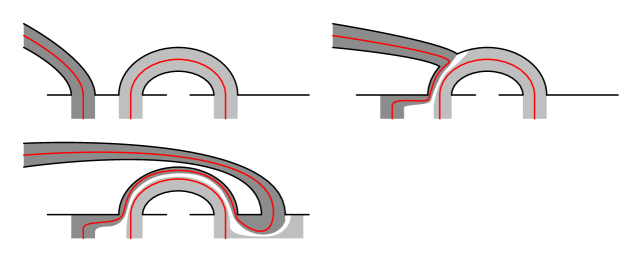
Figure 10. An arcslide diffeomorphism. Top left: the diagram before the arcslide. The two relevant handles are shaded, and their cores ($\alpha$-arcs) are indicated. Top right: an intermediate stage. The images of the handles under the diffeomorphism are shaded and the images of their cores indicated. Bottom right: the diagram after the arcslide. Again, the images of the handles are shaded and the images of their cores indicated.

A key tool for bordered Floer theory (e.g., [LOT14]) is a particular class of diffeomorphisms, the arcslides:

Definition 4.6.

Given an arc diagram $\mathcal{Z}=(\{Z_{i}\},\mathbf{a},M)$ and a pair of adjacent points $a,a^{\prime}\in Z_{i}\cap\mathbf{a}$, let $a^{\prime\prime}$ be a point adjacent to $M(a)$, so that $a^{\prime\prime}$ is above (respectively below) $M(a)$ if $a^{\prime}$ is below (respectively above) $a$. There is a new arc diagram $\mathcal{Z}^{\prime}$ obtained by replacing $a^{\prime}$ by $a^{\prime\prime}$ (and defining $M(a^{\prime\prime})=M(a^{\prime})$). We say that $\mathcal{Z}^{\prime}$ is obtained from $\mathcal{Z}$ by an arcslide.

The surface $F(\mathcal{Z}^{\prime})$ is obtained from $F(\mathcal{Z})$ by sliding one foot of the handle corresponding to $\{a^{\prime},M(a^{\prime})\}$ over the handle corresponding to $\{a,M(a)\}$. In particular, this 1-parameter family of sutured surfaces induces a strongly based diffeomorphism $F(\mathcal{Z}^{\prime})\to F(\mathcal{Z})$, the arcslide diffeomorphism corresponding to sliding $a^{\prime}$ over $a$. See Figure 10 (as well as [ABP09, Section 6.1] and [LOT14, Figure 3]).

Given a half Heegaard diagram $\mathcal{H}=(F,\phi_{L}\nobreak\mskip 2.0mu\mathpunct{}\nonscript\mkern-3.0mu{:}\penalty 300\mskip 6.0mu plus 1.0muF(\mathcal{Z}_{L})\to F,\phi_{R}\nobreak\mskip 2.0mu\mathpunct{}\nonscript\mkern-3.0mu{:}\penalty 300\mskip 6.0mu plus 1.0muF(\mathcal{Z}_{R})\to F)$ and an arcslide diffeomorphism $\psi\nobreak\mskip 2.0mu\mathpunct{}\nonscript\mkern-3.0mu{:}\penalty 300\mskip 6.0mu plus 1.0muF(\mathcal{Z}^{\prime}_{L})\to F(\mathcal{Z}_{L})$ there is a new half Heegaard diagram $(F,\phi_{L}\circ\psi,\phi_{R})$, which we call the result of performing the arcslide to $\mathcal{H}$. In terms of $\alpha$- and $\beta$-arcs, this corresponds to performing an embedded arcslide of the $\alpha$-arc corresponding to $a^{\prime}$ over the $\alpha$-arc corresponding to $a$.

The bordered-sutured manifolds of interest in this paper come from compression bodies, with simple kinds of sutures. We will give a name to that class:

Definition 4.7.

A special bordered-sutured manifold is a bordered-sutured manifold so that each component of $R_{\pm}$ is a bigon with one edge a component of $\Gamma$ and one edge a component of $S_{\pm}$.

The example in Figure 8 is a special bordered-sutured manifold.

Given a bordered 3-manifold with connected boundary, if we view the bordered Heegaard diagram as a bordered-sutured Heegaard diagram then the corresponding bordered-sutured manifold is special, with each $R_{\pm}$ a single bigon. An arced bordered Heegaard diagram with two boundary components (such as the diagrams representing diffeomorphisms [LOT15, Section 5.3]) represents a pair $(Y,\gamma)$ of a cobordism between closed surfaces and an arc $\gamma$ connecting the two boundary components, but does not directly represent a special bordered-sutured manifold. Specifically, we obtain a bordered-sutured diagram by deleting a neighborhood of the arc and viewing the newly-created boundary as sutured arcs; see Figure 11. The corresponding bordered-sutured manifold is $Y\setminus\mathrm{nbd}(\gamma)$ where $R_{+}$ and $R_{-}$ consist of a rectangle each on the cylinder $\partial\mathrm{nbd}(\gamma)$, and $\Gamma$ consists of two arcs along $\partial\mathrm{nbd}(\gamma)$. In particular, this is not a special bordered-sutured manifold. To obtain a special bordered-sutured manifold, we attach a 2-handle to a meridian of $\gamma$ and modify $R_{+}$ and $R_{-}$ to be bigons. At the level of Heegaard diagrams, this can be accomplished by gluing on the tube-cutting diagram shown in Figures 11 and 27. (The tube-cutting diagram appeared previously in [Han16, LT16, AL19].)

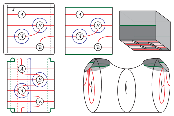
Figure 11. Turning an arced bordered Heegaard diagram into a sutured Heegaard diagram. Top-left: an arced bordered Heegaard diagram for the mapping cylinder of a Dehn twist on a torus. Top-center: the corresponding bordered-sutured diagram. Top-right: the corresponding bordered-sutured manifold, which is not special. Bottom-left: the tube-cutting diagram. Bottom-right: the bordered-sutured manifold represented by the tube-cutting diagram. Gluing this to the manifold on the top-right gives a special bordered-sutured manifold.

There are analogous constructions for bordered $3$-manifolds with more than two boundary components. For example, Figure 12 shows a bordered Heegaard diagram for $(Y,\gamma)$ where $Y$ is the compression body with outer boundary of genus $2$ and inner boundary $T^{2}\amalg T^{2}$ and $\gamma$ is a Y-shaped graph in $Y$ connecting the three boundary components. The figure also shows the corresponding bordered-sutured diagram (which is not special). Gluing on tube-cutting pieces to two of the boundary gives a bordered-sutured Heegaard diagram for a special bordered-sutured structure on $Y$. One can also introduce extra sutured disks, by gluing on the bordered-sutured diagram shown on the right of Figure 12. In particular, from these pieces it is easy to construct a bordered-sutured diagram for any special bordered-sutured structure on a compression body.

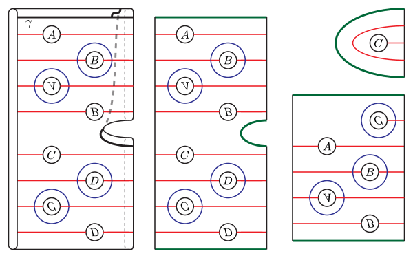
Figure 12. Bordered-sutured diagrams for compression bodies. Left: a bordered Heegaard diagram for $(Y,\gamma)$ where $\gamma$ is a Y-shaped graph connecting the boundary components of $Y$. Center: a bordered-sutured Heegaard diagram $\mathcal{H}$ for a special bordered-sutured structure on $Y$. Right: a bordered-sutured diagram $\mathcal{H}^{\prime}$ so that gluing $\mathcal{H}^{\prime}$ along its left boundary to a boundary component of $\mathcal{H}$ introduces an extra disk suture.

The bordered-sutured modules have several duality properties which allow one to state the pairing theorem in terms of morphism spaces instead of tensor products (cf. [LOT11]). In the general case, the duality properties have the effect of twisting the sutures (see [Zar10]), so we will state them only for special bordered-sutured manifolds:

Theorem 4.8.

Let $Y$ be a special bordered-sutured manifold and $F(\mathcal{Z})$ a component of the bordered boundary of $Y$. Then there is a homotopy equivalence

$$\operatorname{Mor}_{\mathcal{A}(-\mathcal{Z})}\bigl{(}\mathcal{A}(-\mathcal{Z})\boxtimes\mathit{BSD}(Y),\mathcal{A}(-\mathcal{Z})\bigr{)}\simeq\mathit{BSDA}(-Y)$$

where, on the right side, $F(\mathcal{Z})$ is treated as type $A$ boundary and the other components as type $D$ boundary.

In particular, given another bordered-sutured manifold $Y^{\prime}$ and an identification of $F(\mathcal{Z})$ with one of the boundary components of $Y^{\prime}$,

$$\operatorname{Mor}_{\mathcal{A}(-\mathcal{Z})}\bigl{(}\mathit{BSD}(Y),\mathit{BSD}(Y^{\prime})\bigr{)}\simeq\mathit{BSD}((-Y)\cup_{F(\mathcal{Z})}Y^{\prime}).$$

Proof.

The proof is the same as the proof of [AL19, Theorem 2.6] (most of the work of which is in [Zar10]), observing that the twisting slice acts trivially on a special bordered-sutured manifold. The second statement follows from the first by tensoring both sides with $\mathit{BSD}(Y^{\prime})$. ∎

Versions of Theorem 4.8 where the other boundary components of $Y$ or $Y^{\prime}$ are treated as type $A$ rather than $D$ boundary follow from the same proof or, in many cases, by tensoring with the type $\mathit{AA}$ identity bimodule.

4.3. Twisted bordered-sutured Floer homology

Bordered-sutured Floer homology with twisted coefficients is not developed in Zarev’s papers, but is a straightforward combination of his theory with Ozsváth-Szabó’s construction of $\widehat{\mathit{HF}}$ with twisted coefficients. The group of periodic domains $\pi_{2}(\mathbf{x},\mathbf{x})$ in a bordered-sutured Heegaard diagram representing $(Y,\Gamma,\phi\nobreak\mskip 2.0mu\mathpunct{}\nonscript\mkern-3.0mu{:}\penalty 300\mskip 6.0mu plus 1.0muF(\mathcal{Z})\to\partial Y)$ is isomorphic to $H_{2}(Y,\phi(F(\mathcal{Z})))$ [Zar09, p. 24]. Note that $\phi(F(\mathcal{Z}))$ is the bordered boundary of $Y$, so in particular has no closed components; abusing notation, we will use $F$ to denote the image $\phi(F)\subset\partial Y$. Thus, one can define the twisted bordered-sutured modules $\underline{\mathit{BSD}}(Y)$ and $\underline{\mathit{BSA}}(Y)$, similarly to the construction of $\widehat{\underline{{\mathit{CF}}}}$ above. (The bordered case is discussed in [LOT18, Sections 6.4 and 7.4].) Specifically, we can view $\mathcal{A}(\mathcal{Z})\otimes\mathbb{F}_{2}[H_{2}(Y,F)]$ as a dg algebra over $\mathbb{F}_{2}[H_{2}(Y,F)]$. Then the invariant $\underline{\mathit{BSD}}(Y)$ is a type $D$ structure over $\mathcal{A}(-\mathcal{Z})\otimes\mathbb{F}_{2}[H_{2}(Y,F)]$, while $\underline{\mathit{BSA}}(Y)$ is a (strictly unital) $A_{\infty}$-module over $\mathcal{A}(\mathcal{Z})\otimes\mathbb{F}_{2}[H_{2}(Y,F)]$. The fact that $\mathcal{A}(\mathcal{Z})\otimes\mathbb{F}_{2}[H_{2}(Y,F)]$ is viewed as a dg algebra over the ground ring $\mathbb{F}_{2}[H_{2}(Y,F)]$ means, in particular, that the operations on $\underline{\mathit{BSA}}(Y)$ satisfy $m_{1+n}(x,a_{1},\dots,e^{h}a_{i},\dots,a_{n})=e^{h}m_{1+n}(x,a_{1},\dots,a_{i},\dots,a_{n})$ for any $e^{h}\in\mathbb{F}_{2}[H_{2}(Y,F)]$, so strict unitality implies that $m_{1+n}(x,a_{1},\dots,e^{h},\dots,a_{n})=0$ if $n>1$. The formulas for the twisted operations are obtained easily from the untwisted case. For example, for $\underline{\mathit{BSA}}(Y)$, one replaces Zarev’s formula [Zar09, Definition 7.12] by

$$m_{k}(\mathbf{x},a_{1},\dots,a_{k-1})=\sum_{\begin{subarray}{c}\mathbf{y}\in\mathcal{G}(x,y)\\ \vec{a}(\mathbf{x},\mathbf{y},\vec{\rho})=a_{1}\otimes\dots\otimes a_{k-1}\\ \operatorname{ind}(B,\vec{\rho})=1\end{subarray}}\Bigl{(}\#\mathcal{M}^{B}_{\mathit{emb}}(\mathbf{x},\mathbf{y};\vec{\rho})\Bigr{)}e^{[B_{\mathbf{x}}*B*B_{\mathbf{y}}^{-1}]}\mathbf{y},$$

where $B_{\mathbf{x}}$ and $B_{\mathbf{y}}$ are domains connecting the generators to the basepoint, as in the definition of $\widehat{\underline{{\mathit{CF}}}}$. (Also as in the definition of $\widehat{\underline{{\mathit{CF}}}}$, one fixes one choice of base generator for each $\mathrm{spin}^{c}$-structure.)

One can equivalently view $\underline{\mathit{BSA}}(Y)$ as an $A_{\infty}$-bimodule over $\mathbb{F}_{2}[H_{2}(Y,F)]$ and $\mathcal{A}(\mathcal{Z})$, and $\underline{\mathit{BSD}}(Y)$ as a type $\mathit{DA}$ bimodule over $\mathcal{A}(-\mathcal{Z})$ and $\mathbb{F}_{2}[H_{2}(Y,F)]$. In both cases, the bimodule structure is quite simple: for $\underline{\mathit{BSA}}(Y)$, $m_{m,1,n}$ vanishes if $m$ and $n$ are both positive, or if $m>1$ and $n=0$. For $\underline{\mathit{BSD}}(Y)$, $\delta^{1}_{1+n}$ is only non-zero for $n=0,1$ and the operation $\delta^{1}_{2}$ is given by $\delta^{1}_{2}(\mathbf{x},e^{h})=\iota\otimes(e^{h}\mathbf{x})$ (where $\iota$ is the basic idempotent with $\iota\mathbf{x}=\mathbf{x}$).

There are also partially twisted versions of the bordered-sutured modules. Focusing on $\underline{\mathit{BSA}}$, say, given a module $M$ over $\mathbb{F}_{2}[H_{2}(Y,F)]$, the bordered-sutured complex twisted by $M$ is

$$\underline{\mathit{BSA}}(Y;M)=M\otimes_{\mathbb{F}_{2}[H_{2}(Y,F)]}\underline{\mathit{BSA}}(Y).$$

A particularly interesting case is when $F_{0}$ is a union of components of the bordered boundary of $Y$ and $M=\mathbb{F}_{2}[H_{1}(F_{0})]$ is an algebra over $\mathbb{F}_{2}[H_{2}(Y,F)]$ via the connecting homomorphism $H_{2}(Y,F)\to H_{1}(F)$ and projection $H_{1}(F)\to H_{1}(F_{0})$.

The twisted versions $\underline{\mathit{BSDA}}(Y)$ and $\underline{\mathit{BSDA}}(Y;M)$ of $\mathit{BSDA}(Y)$ are defined similarly.

We state the twisted-coefficient pairing theorem for the invariant $\mathit{BSDA}$, since the other versions are special cases:

Theorem 4.9.

Let $Y$ be the result of gluing bordered-sutured $3$-manifolds $Y_{1}$ and $Y_{2}$ along a union of bordered boundary components $F(\mathcal{Z}^{\prime})$. Let $F_{i}$ denote the full bordered boundary of $Y_{i}$ and $F$ the bordered boundary of $Y$. View $F(Z^{\prime})$ as type $A$ bordered boundary of $Y_{1}$ and view $F(-Z^{\prime})$ as type $D$ bordered boundary of $Y_{2}$. Let $M_{i}$ be a module over $\mathbb{F}_{2}[H_{2}(Y_{i},F_{i})]$. Then

(4.10) $$\underline{\mathit{BSDA}}(Y_{1};M_{1}){}^{\mathcal{A}(Z^{\prime})}\mskip-1.80002mu\boxtimes_{\mathcal{A}(Z^{\prime})}\underline{\mathit{BSDA}}(Y_{2};M_{2})\simeq\underline{\mathit{BSDA}}(Y;M_{1}\otimes M_{2})$$

where $M_{1}\otimes M_{2}$ is a module over $\mathbb{F}_{2}[H_{2}(Y,F)]$ via the ring homomorphism $\mathbb{F}_{2}[H_{2}(Y,F)]\to\mathbb{F}_{2}[H_{2}(Y_{1},F_{1})]\otimes\mathbb{F}_{2}[H_{2}(Y_{2},F_{2})]$ induced by the homomorphism $H_{2}(Y,F)\to H_{2}(Y_{1},F_{1})\oplus H_{2}(Y_{2},F_{2})$ induced by the maps of pairs $(Y,F)\to(Y,F_{i}\cup Y_{j})$ and excision $H_{2}(Y,F_{i}\cup Y_{j})\cong H_{2}(Y_{i},F_{i})$, where $\{i,j\}=\{1,2\}$.

The proof is the same as, for instance, [LOT18, Theorem 9.44] (see also [LOT15, Theorem 12]). A key point is that a periodic domain for $Y$ restricts to periodic domains for $Y_{1}$ and $Y_{2}$; this corresponds to the map $H_{2}(Y,F)\to H_{2}(Y_{1},F_{1})\oplus H_{2}(Y_{2},F_{2})$ above. Choosing paths $B_{\mathbf{x}}$ for $Y$ as in Section 4.1 gives a partial choice of paths for the $Y_{i}$, compatible along the boundary; these can then be extended to complete choices for the $Y_{i}$ and used to define the twisted coefficient complexes.

For example, if $M_{i}=\mathbb{F}_{2}[H_{2}(Y_{i},F_{i})]$, then Formula (4.10) computes $\underline{\mathit{BSDA}}(Y;\mathbb{F}_{2}[H_{2}(Y,F_{1}\cup F_{2})])$, not $\underline{\mathit{BSDA}}(Y;\mathbb{F}_{2}[H_{2}(Y,F)])$. (The difference is that $F_{1}\cup F_{2}$ includes the part of $\partial Y_{i}$ where $Y_{1}$ and $Y_{2}$ are glued together, which is not part of $\partial Y$.) However, there is an evident split injection $H_{2}(Y,F)\hookrightarrow H_{2}(Y,F_{1}\cup F_{2})$. If one chooses a splitting $p\nobreak\mskip 2.0mu\mathpunct{}\nonscript\mkern-3.0mu{:}\penalty 300\mskip 6.0mu plus 1.0muH_{2}(Y,F_{1}\cup F_{2})\to H_{2}(Y,F)$ then we can form the tensor product

(4.11) $$\underline{\mathit{BSDA}}(Y;\mathbb{F}_{2}[H_{2}(Y,F_{1}\cup F_{2})])\otimes_{\mathbb{F}_{2}[H_{2}(Y,F_{1}\cup F_{2})]}\mathbb{F}_{2}[H_{2}(Y,F)]\simeq\underline{\mathit{BSDA}}(Y).$$

So, the pairing theorem determines the standard, totally twisted bimodule of $Y$ via the two-step process of taking the box product and then extending scalars under $p_{*}$.

As a special case of Theorem 4.9, if some component(s) $F_{0}$ of $\partial Y$ are parameterized by $F(\mathcal{Z}_{0})$ then

(4.12) $$\underline{\mathit{BSDA}}(Y;\mathbb{F}_{2}[H_{1}(F_{0})])\simeq\mathit{BSDA}(Y)\boxtimes\underline{\mathit{BSDA}}(\mathit{Id}_{\mathcal{Z}_{0}}).$$

So, one can reconstruct the boundary twisted version of $\mathit{BSDA}$ from the untwisted version. (In particular, the boundary twisting is, in some sense, redundant with the bordered module structure.)

Finally, we state the Künneth theorem for bordered-sutured Floer homology. (Note that one cannot apply the statement below directly to an arced bordered manifold with two boundary components: one must first replace it by a bordered-sutured manifold, which then has connected boundary.)

Theorem 4.13.

Consider an (internal) connected sum of two bordered-sutured 3-manifolds, $(Y_{1},F_{1})$ and $(Y_{2},F_{2})$.

• If $\partial Y_{1}\neq\emptyset$ but $\partial Y_{2}=\emptyset$ then

  $$\mathit{BSD}(Y_{1}\#Y_{2}) \simeq\mathit{BSD}(Y_{1})\otimes_{\mathbb{F}_{2}}\widehat{\mathit{CF}}(Y_{2})$$

  $$\underline{\mathit{BSD}}(Y_{1}\#Y_{2}) \simeq\underline{\mathit{BSD}}(Y_{1})\otimes_{\mathbb{F}_{2}}\widehat{\underline{{\mathit{CF}}}}(Y_{2}).$$

  Here, the second homotopy equivalence uses the evident isomorphism $H_{2}(Y_{1}\#Y_{2},F_{1})\cong H_{2}(Y_{1},F_{1})\oplus H_{2}(Y_{2})$.

• If $\partial Y_{1}\neq\emptyset$ and $\partial Y_{2}\neq\emptyset$ then

  $$\mathit{BSD}(Y_{1}\#Y_{2}) \simeq\mathit{BSD}(Y_{1})\otimes_{\mathbb{F}_{2}}\mathit{BSD}(Y_{2})\otimes_{\mathbb{F}_{2}}\widehat{\mathit{CF}}(S^{2}\times S^{1})$$

  $$\underline{\mathit{BSD}}(Y_{1}\#Y_{2},F_{1}\amalg F_{2}) \simeq\underline{\mathit{BSD}}(Y_{1})\otimes_{\mathbb{F}_{2}}\underline{\mathit{BSD}}(Y_{2})\otimes_{\mathbb{F}_{2}}\widehat{\underline{{\mathit{CF}}}}(S^{2}\times S^{1}).$$

  Here, the second homotopy equivalence uses the evident isomorphism $H_{2}(Y_{1}\#Y_{2},F_{1}\amalg F_{2})\cong H_{2}(Y_{1},F_{1})\oplus H_{2}(Y_{2},F_{2})\oplus\mathbb{Z}\cong H_{2}(Y_{1},F_{1})\oplus H_{2}(Y_{2},F_{2})\oplus H_{2}(S^{2}\times S^{1})$. (Recall that the $F_{i}$ are just the bordered parts of the boundary, so have no closed components.)

Proof.

All of these statements follow easily by taking the (internal) connected sum of Heegaard diagrams for $Y_{1}$ and $Y_{2}$ near a suture (basepoint). In the second case, to obtain a Heegaard diagram for $Y$, we then have to add a pair of $\alpha$- and $\beta$-circles inside the connected sum neck, which gives the extra $\widehat{\mathit{CF}}(S^{2}\times S^{1})$ factor. ∎

4.4. Twisted sutured Floer homology

Here, we collect some properties we need of twisted sutured Floer homology. Twisted sutured Floer homology can be viewed as a special case of twisted bordered-sutured Floer homology, in which the bordered boundary is empty. More directly, given a balanced sutured manifold $(Y,\Gamma)$, there is a twisted sutured Floer complex $\underline{\mathit{SFC}}(Y,\Gamma)$ over $\mathbb{F}_{2}[H_{2}(Y)]$, extending the untwisted case [Juh06], defined as follows. Given a sutured Heegaard diagram $\mathcal{H}=(\Sigma,\boldsymbol{\alpha},\boldsymbol{\beta})$ for $(Y,\Gamma)$ and a point $\mathbf{x}_{0}\in T_{\alpha}\cap T_{\beta}$, there is a map $\pi_{2}(\mathbf{x}_{0},\mathbf{x}_{0})\to H_{2}(Y)$, which we denote $B\mapsto[B]$ [Juh06, Definition 3.9]. (If the Heegaard diagram is sufficiently stabilized, or we work in the cylindrical setting, this map is an isomorphism.) The complex $\underline{\mathit{SFC}}(Y,\Gamma)$ is freely generated over $\mathbb{F}_{2}[H_{2}(Y)]$ by $T_{\alpha}\cap T_{\beta}$ with differential as in Formula (4.1) (without the requirement on $n_{z}$, since sutured Heegaard diagrams have punctures instead of basepoints). Given an $\mathbb{F}_{2}[H_{2}(Y)]$-module $M$, $\underline{\mathit{SFC}}(Y,\Gamma;M)$, $\underline{\mathit{SFH}}(Y,\Gamma)$, and $\underline{\mathit{SFH}}(Y,\Gamma;M)$ are defined as in the closed case.

The key property of sutured Floer homology is its behavior under surface decompositions. The twisted version of Juhász’s surface decomposition theorem [Juh08, Theorem 1.3] is:

Proposition 4.14.

Let $(Y,\Gamma)$ be a balanced sutured manifold, $S\subset Y$ a good decomposing surface [Juh08, Defintion 4.6], and $M$ a module over $\mathbb{F}_{2}[H_{2}(Y)]$. Let $(Y^{\prime},\Gamma^{\prime})$ be the result of decomposing $(Y,\Gamma)$ along $S$. Then there is a module $M^{\prime}$ over $\mathbb{F}_{2}[H_{2}(Y^{\prime})]$ so that

$$\underline{\mathit{SFH}}(Y^{\prime},\Gamma^{\prime};M^{\prime})\cong\bigoplus_{\mathfrak{s}\text{ outer w.r.t.\ }S}\underline{\mathit{SFH}}(Y,\Gamma;\mathfrak{s};M).$$

Moreover, as abelian groups, $M^{\prime}\cong M$.

Proof.

We adapt Zarev’s proof of the sutured decomposition theorem [Zar09, Theorem 10.5], and will assume some familiarity with it. (Zarev’s figure [Zar09, Figure 10] is perhaps especially enlightening.) Decompose

(4.15) $$Y=(S\times[-2,2])\cup_{S\times\{\pm 2\}}W.$$

Viewing $S\times[-2,2]$ as the identity cobordism of the sutured surface $S$ makes it into a bordered-sutured manifold; make $W$ into a bordered-sutured manifold so that Equation (4.15) holds as sutured manifolds. There is a bordered-sutured structure on $S\times([-2,-1]\cup[1,2])$ so that

(4.16) $$Y^{\prime}=(S\times\left([-2,-1]\cup[1,2]\right))\cup_{S\times\{\pm 2\}}W$$

as sutured manifolds; see Zarev’s paper for an explicit description. Moreover, for these bordered-sutured structures,

(4.17) $$\mathit{BSD}(S\times\left([-2,-1]\cup[1,2]\right),\mathfrak{s}_{k}^{\prime})\cong\mathit{BSD}(S\times[-2,2],\mathfrak{s}_{k})$$

where $\mathfrak{s}_{k}$ is the $\mathrm{spin}^{c}$-structure on $S\times[-2,2]$ so that in the corresponding idempotents for $\mathit{BSD}(S\times[-2,2])$, all the $\alpha$-arcs corresponding to $S\times\{-2\}$ are occupied, and none corresponding to $S\times\{2\}$ are; and $\mathfrak{s}_{k}^{\prime}$ is the $\mathrm{spin}^{c}$-structure on $S\times[-2,-1]\cup[1,2]$ which agrees with $\mathfrak{s}_{k}$ on $S\times\{\pm 2\}$. (See Zarev’s paper for a little more discussion.)

Combining the long exact sequence for the pair $(Y,S\times[-2,2])$ and the excision isomorphism $H_{*}(Y,S\times[-2,2])\cong H_{*}(W,S\times\{-2,2\})$ gives

$$0=H_{2}(S)\to H_{2}(Y)\to H_{2}(W,S\times\{-2,2\})\to H_{1}(S)\to\cdots.$$

Since $H_{1}(S)$ is free, we can choose a splitting $p\nobreak\mskip 2.0mu\mathpunct{}\nonscript\mkern-3.0mu{:}\penalty 300\mskip 6.0mu plus 1.0muH_{2}(W,S\times\{-2,2\})\to H_{2}(Y)$. Let $M_{W}=p^{*}M$ be the module over $\mathbb{F}_{2}[H_{2}(W,S\times\{-2,2\})]$ obtained by restricting scalars. Equation (4.15) and the twisted pairing theorem, Theorem 4.9, give

$$\underline{\mathit{SFC}}(Y,\Gamma;\mathfrak{s}_{W}\cup\mathfrak{s}_{S};M)\simeq\underline{\mathit{BSA}}(W;\mathfrak{s}_{W};M_{W})\boxtimes\mathit{BSD}(S\times[-2,2],\mathfrak{s}_{S}).$$

The outer $\mathrm{spin}^{c}$-structures on $Y$ are the ones that restrict to $\mathfrak{s}_{k}$ on $S\times[-2,2]$, so in particular

(4.18) $$\bigoplus_{\mathfrak{s}\text{ outer w.r.t.\ }S}\underline{\mathit{SFC}}(Y,\Gamma;\mathfrak{s};M)\simeq\bigoplus_{\mathfrak{s}_{W}}\underline{\mathit{BSA}}(W,\mathfrak{s}_{W};M_{W})\boxtimes\mathit{BSD}(S\times[-2,2],\mathfrak{s}_{k}).$$

Since $\mathit{BSD}(S\times[-2,2],\mathfrak{s}_{k})$ is supported on the idempotent where all the arcs corresponding to $S\times\{-2\}$ are occupied, and none corresponding to $S\times\{2\}$ are, the box tensor product on the right vanishes unless $\mathfrak{s}_{W}$ has the same property. So, we could restrict the direct sum to these $\mathrm{spin}^{c}$-structures, which we could again call outer.

The homeomorphism $Y^{\prime}\cong W$ induces a map $i\nobreak\mskip 2.0mu\mathpunct{}\nonscript\mkern-3.0mu{:}\penalty 300\mskip 6.0mu plus 1.0muH_{2}(Y^{\prime})\to H_{2}(W,S\times\{-2,2\})$. Let $M^{\prime}=i^{*}M_{W}$. By Equation (4.16) and the twisted pairing theorem,

(4.19) $$\bigoplus_{\mathfrak{s}^{\prime}}\underline{\mathit{SFC}}(Y^{\prime},\Gamma^{\prime};\mathfrak{s}^{\prime};M^{\prime})\simeq\bigoplus_{\mathfrak{s}_{W}}\underline{\mathit{BSA}}(W,\mathfrak{s}_{W};M_{W})\boxtimes\mathit{BSD}(S\times([-2,-1]\cup[1,2]),\mathfrak{s}_{k}^{\prime}).$$

Combining Equations (4.17), (4.18), and (4.19) gives the result. ∎

Recall that an irreducible balanced sutured manifold is taut if $R(\gamma)$ is Thurston-norm minimizing in $H_{2}(Y,\Gamma)$.

Corollary 4.20.

If $(Y,\Gamma)$ is a taut balanced sutured manifold and $M$ is a nontrivial module over $\mathbb{Z}[H_{2}(Y)]$ then $\underline{\mathit{SFH}}(Y,\Gamma;M)$ is nontrivial. In fact, $\underline{\mathit{SFH}}(Y,\Gamma;M)$ has a summand isomorphic to $M$ as an abelian group.

Proof.

The proof is the same as Juhász’s proof in the untwisted case [Juh08, Theorem 1.4], using Proposition 4.14 in place of the untwisted surface decomposition theorem. ∎

The Künneth theorem holds for balanced sutured manifolds for either disjoint unions or boundary connected sums. (These operations differ by a disk decomposition.) For ordinary connected sums, we have:

Lemma 4.21.

[Juh06, Proposition 9.15]

1. Suppose that $Y_{1}$ is a closed $3$-manifold and $(Y_{2},\Gamma_{2})$ is a balanced sutured 3-manifold. Then $\mathit{SFH}(Y_{1}\#Y_{2},\Gamma_{2})\cong\widehat{\mathit{HF}}(Y_{1})\otimes\mathit{SFH}(Y_{2},\Gamma_{2})$. Moreover, given modules $M_{i}$ over $\mathbb{Z}[H_{2}(Y_{i})]$, $\underline{\mathit{SFH}}(Y_{1}\#Y_{2},\Gamma_{2};M_{1}\otimes M_{2})\cong\widehat{\underline{\mathit{HF}}}(Y_{1};M_{1})\otimes\underline{\mathit{SFH}}(Y_{2},\Gamma_{2};M_{2})$ as modules over $\mathbb{Z}[H_{2}(Y_{1}\#Y_{2})]\cong\mathbb{Z}[H_{2}(Y_{1})]\otimes\mathbb{Z}[H_{2}(Y_{2})]$.

2. Suppose $(Y_{i},\Gamma_{i})$, $i=1,2$, is a balanced sutured manifold. Then $\mathit{SFH}(Y_{1}\#Y_{2},\Gamma_{1}\cup\Gamma_{2})\cong\mathit{SFH}(Y_{1},\Gamma_{1})\otimes\mathit{SFH}(Y_{2},\Gamma_{2})\otimes\widehat{\mathit{HF}}(S^{2}\times S^{1})$. Moreover, given modules $M_{i}$ over $\mathbb{Z}[H_{2}(Y_{i})]$ and a module $M$ over $\mathbb{Z}[t,t^{-1}]$, if we identify $H_{2}(Y_{1}\#Y_{2})\cong H_{2}(Y_{1})\oplus H_{2}(Y_{2})\oplus\mathbb{Z}$ where the third summand is generated by the connected sum sphere, then $\underline{\mathit{SFH}}(Y_{1}\#Y_{2},\Gamma_{1}\cup\Gamma_{2};M_{1}\otimes M_{2}\otimes M)\cong\underline{\mathit{SFH}}(Y_{1},\Gamma_{1};M_{1})\otimes\underline{\mathit{SFH}}(Y_{2},\Gamma_{2};M_{2})\otimes\widehat{\underline{\mathit{HF}}}(S^{2}\times S^{1};M)$.

Proof.

The untwisted cases were proved by Juhász [Juh06, Proposition 9.15]; the twisted cases follow from the same arguments. ∎

Juhász showed (combining [Juh06, Proposition 9.18] and [Juh08, Theorem 1.4]) that in the untwisted case, for an irreducible, balanced sutured manifold $(Y,\Gamma)$, $\mathit{SFH}(Y,\Gamma)\neq 0$ if and only if $(Y,\Gamma)$ is taut. We give an indirect proof that, given $Y$, $\Gamma$ can always be chosen satisfying this property:

Proposition 4.22.

For any 3-manifold $Y$ with boundary there is a choice of sutures $\Gamma\subset\partial Y$ so that $\mathit{SFH}(Y,\Gamma)\neq 0$. Moreover, $\Gamma$ can be chosen so that for each component of $\partial Y$, $\chi(R_{+})=\chi(R_{-})$.

Proof.

Fix some parameterization of $\partial Y$ by $F(\mathcal{Z})$ for some arc diagram $\mathcal{Z}$ making $Y$ into a special bordered-sutured manifold with a single suture on each boundary, say. If we fix some filling $Y^{\prime}$ of the boundary components of $Y$ by handlebodies $H_{1},\dots,H_{n}$ then

(4.23) $$\mathit{BSA}(Y)\boxtimes\bigl{(}\mathit{BSD}(H_{1})\otimes\cdots\otimes\mathit{BSD}(H_{n})\bigr{)}\simeq\widehat{\mathit{CF}}(Y^{\prime})\otimes(\mathbb{F}_{2}\oplus\mathbb{F}_{2})^{\otimes(n-1)}$$

(since the right side corresponds to a manifold with $n$ $S^{2}$ boundary components). Since $\widehat{\mathit{HF}}$ is always nontrivial (by the computation of its Euler characteristic if $b_{1}=0$ and detection of the Thurston norm if $b_{1}>0$), it follows that $\mathit{BSA}(Y)\not\simeq 0$. Thus, there is some idempotent $\iota$ so that $\mathit{BSA}(Y)\cdot\iota\not\simeq 0$. Moreover, in the tensor product (4.23), the only $\mathrm{spin}^{c}$-structure on $\partial H_{i}$ which extends over $H_{i}$ is the middle $\mathrm{spin}^{c}$-structure (the one with $\langle c_{1}(\mathfrak{s}),[\partial H_{i}]\rangle=0$). So, we can assume the idempotent $\iota$ occupies half of the $\alpha$-arcs corresponding to each boundary component of $Y$.

Zarev showed that for each idempotent $\iota$ there is a choice of sutures $\Gamma_{\iota}$ on $\partial Y$ so that $\mathit{BSA}(Y)\cdot\iota\simeq\mathit{SFC}(Y,\Gamma_{\iota})$ [Zar10, Section 6.1]. The region $R_{+}$ on each boundary component is the union of a disk and a strip corresponding to each $\alpha$-arc occupied by $\iota$. Since half the $\alpha$-arcs are occupied in $\iota$, the Euler characteristic is half of the Euler characteristic of the boundary component. ∎

Notice that Proposition 4.22 is constructive: given $\mathcal{Z}$, there is an explicit, finite list of possibilities for $\Gamma$.

5. Support of Heegaard Floer homology and detection of handlebodies

5.1. Definitions of the support

In this section, we recall the classical definition of the support, and then give several equivalent definitions of the support of bordered-sutured Floer homology. Only the classical case is needed for Section 5, so the reader interested only in Theorem 1.1 might read the next paragraph and then skip to Section 5.2.

We recall the classical definition of the support of a module. Given a module $M$ over a commutative ring $R$, let $\operatorname{Ann}(M)=\{r\in R\mid rm=0\ \forall m\in M\}$ denote the annihilator of $M$, and let $V(\operatorname{Ann}(M))$ be the set of prime ideals in $R$ containing $\operatorname{Ann}(M)$ (a subvariety of $\operatorname{Spec}(R)$). The support of $M$, $\operatorname{Supp}(M)$, is the set of prime ideals $I\subset R$ so that $M_{I}\neq 0$ (where $M_{I}$ denotes $M$ localized at $I$, that is, with all elements of $R$ not lying in $I$ inverted). If $M$ is finitely generated then $\operatorname{Supp}(M)=V(\operatorname{Ann}(M))$ [Mat89, pp. 25–26]. In particular, since $\widehat{\underline{\mathit{HF}}}(Y)$ is finitely generated over $R=\mathbb{F}_{2}[H_{2}(Y)]\cong\mathbb{F}_{2}[x_{1}^{\pm 1},\dots,x_{n}^{\pm 1}]$, $\operatorname{Supp}(\widehat{\underline{\mathit{HF}}}(Y))=V(Ann\widehat{\underline{\mathit{HF}}}(Y))$, and similarly for twisted sutured Floer homology.

The rest of this section, about the support of the bordered-sutured modules, is not needed until Section 6. Given a bordered-sutured 3-manifold $(Y,\Gamma,\phi\nobreak\mskip 2.0mu\mathpunct{}\nonscript\mkern-3.0mu{:}\penalty 300\mskip 6.0mu plus 1.0muF(\mathcal{Z})\to\partial Y)$ with $H_{2}(Y,F)\cong\mathbb{Z}^{n}$, the totally twisted bordered-sutured module $\underline{\mathit{BSD}}(Y)$ is a module over $\mathcal{A}(\mathcal{Z})\otimes\mathbb{F}_{2}[H_{2}(Y,F)]\cong\mathcal{A}(\mathcal{Z})\otimes\mathbb{F}_{2}[x_{1}^{\pm 1},\dots,x_{n}^{\pm 1}]$. The support of $\underline{\mathit{BSD}}(Y)$ is the set of prime ideals in

$$R=\mathbb{F}_{2}[H_{2}(Y,F)]\cong\mathbb{F}_{2}[x_{1}^{\pm 1},\dots,x_{n}^{\pm 1}]$$

so that $R_{I}\otimes_{R}\underline{\mathit{BSD}}(Y)$ is not chain homotopy equivalent to the trivial module. This condition has several equivalent formulations:

Lemma 5.1.

The following conditions on a prime ideal $I\subset R$ are equivalent:

1. The module $R_{I}\otimes_{R}\underline{\mathit{BSD}}(Y)$ is chain homotopy equivalent to the trivial module.

2. The homology of $R_{I}\otimes_{R}\underline{\mathit{BSD}}(Y)$ vanishes.

3. The tensor product $R_{I}\otimes_{R}H_{*}\underline{\mathit{BSD}}(Y)$ vanishes.

Proof.

Obviously Condition (1) implies Condition (2). Quasi-isomorphism and homotopy equivalence agree for type $D$ structures which are homotopy equivalent to bounded ones (as $\mathit{BSD}(Y)$ and $\underline{\mathit{BSD}}(Y)$ are) [LOT15, Corollary 2.4.4]. So, Condition (2) implies Condition (1), since Condition (2) implies the inclusion of the trivial module is a quasi-isomorphism. The equivalence of Conditions (2) and (3) follows from the fact that homology commutes with localization. ∎

We can obtain the same object by quotienting by the augmentation ideal in $\mathcal{A}(\mathcal{Z})$. That is, let $\mathcal{I}(\mathcal{Z})$ be the direct sum over basic idempotents $\iota$ of $\mathbb{F}_{2}$; $\mathcal{I}(\mathcal{Z})$ is the usual ground ring for $\mathcal{A}(\mathcal{Z})$. There is an augmentation $\mathcal{A}(\mathcal{Z})\to\mathcal{I}(\mathcal{Z})$ which sends all Reeb chords to $0$; this makes $\mathcal{I}(\mathcal{Z})$ into an $A_{\infty}$ $\mathcal{A}(\mathcal{Z})$-module (where almost all $A_{\infty}$-operations vanish). Given a bordered-sutured manifold $Y$ as above, we can then form a chain complex $\mathcal{I}(\mathcal{Z})\boxtimes_{\mathcal{A}(\mathcal{Z})}\underline{\mathit{BSD}}(Y)$ over $R$; this is the result of quotienting $\underline{\mathit{BSD}}(Y)$ by the augmentation ideal in $\mathcal{A}(\mathcal{Z})$.

Proposition 5.2.

The support of $\underline{\mathit{BSD}}(Y)$ is the same as the support of the $R$-module $H_{*}\bigl{(}\mathcal{I}(\mathcal{Z})\boxtimes_{\mathcal{A}(\mathcal{Z})}\underline{\mathit{BSD}}(Y)\bigr{)}$.

Proof.

First, suppose that $I\not\in\operatorname{Supp}(\underline{\mathit{BSD}}(Y))$. Then $\underline{\mathit{BSD}}(Y)\otimes R_{I}$ is homotopy equivalent to the trivial module, so $(\mathcal{I}(\mathcal{Z})\otimes R)\boxtimes\underline{\mathit{BSD}}(Y)\otimes R_{I}$ is homotopy equivalent to the trivial complex, so $I$ is not in the support of $H_{*}\bigl{(}\mathcal{I}(\mathcal{Z})\boxtimes\underline{\mathit{BSD}}(Y)\bigr{)}$.

Conversely, suppose that $I\not\in\operatorname{Supp}H_{*}\bigl{(}\mathcal{I}(\mathcal{Z})\boxtimes\underline{\mathit{BSD}}(Y)\bigr{)}$. Decompose the algebra $\mathcal{A}(\mathcal{Z})$ as $\mathcal{I}\oplus\mathcal{A}_{+}$, where $\mathcal{A}_{+}$ is the augmentation ideal. Using the basis given by the generators, view the differential on $\underline{\mathit{BSD}}(Y)\otimes R_{I}$ as a matrix $A$ and decompose $A=A_{0}+A_{+}$ where the entries of $A_{0}$ are in $\mathcal{I}\otimes R_{I}$ and the entries of $A_{+}$ are in $\mathcal{A}_{+}\otimes R_{I}$. The hypothesis on $I$ is equivalent to $A_{0}$ being invertible over $\mathcal{I}\otimes R_{I}$. (More precisely, there is a matrix $B_{0}$ so that $A_{0}B_{0}$ and $B_{0}A_{0}$ are diagonal with basic idempotents on the diagonal.) The matrix $A_{+}$ is nilpotent (because $\mathcal{A}_{+}$ is), so $A$ is also invertible. Thus, $\underline{\mathit{BSD}}(Y)\otimes R_{I}$ is contractible, so $I\not\in\operatorname{Supp}\underline{\mathit{BSD}}(Y)$, as desired. ∎

Note that, given a bordered-sutured Heegaard diagram $\mathcal{H}$ for $Y$, $\mathcal{I}(\mathcal{Z})\boxtimes_{\mathcal{A}(\mathcal{Z})}\underline{\mathit{BSD}}(\mathcal{H})$ is isomorphic, as a chain complex over $\mathcal{I}(\mathcal{Z})\otimes R$, to $\underline{\mathit{BSA}}(\mathcal{H})$, where we view $\underline{\mathit{BSA}}(\mathcal{H})$ as a module over $\mathcal{I}(\mathcal{Z})\otimes R$ by restriction of scalars.

Because nontrivial algebra elements act by zero on $\mathcal{I}(\mathcal{Z})\boxtimes_{\mathcal{A}(\mathcal{Z})}\underline{\mathit{BSD}}(\mathcal{H})$, the module is in fact induced from a module over $\mathbb{F}_{2}[H_{2}(Y)]$ via the inclusion $\mathbb{F}_{2}[H_{2}(Y)]\hookrightarrow\mathbb{F}_{2}[H_{2}(Y,F)]$. This is slightly easier to see for $\underline{\mathit{BSA}}(\mathcal{H})$. Recall that as an $A_{\infty}$-module, $\underline{\mathit{BSA}}(\mathcal{H})$ decomposes along $\mathrm{spin}^{c}$-structures, as

$$\underline{\mathit{BSA}}(\mathcal{H})\simeq\bigoplus_{\mathfrak{s}\in\mathrm{spin}^{c}(Y)}\underline{\mathit{BSA}}(\mathcal{H},\mathfrak{s}).$$

We can also consider relative $\mathrm{spin}^{c}$-structures $\mathrm{spin}^{c}(Y,\partial Y)$ extending any given $\mathrm{spin}^{c}$-structure on $\partial Y$, and as a chain complex over $\mathcal{I}(\mathcal{Z})\otimes R$ we have a decomposition

$$\underline{\mathit{BSA}}(\mathcal{H})\simeq\bigoplus_{\mathfrak{t}\in\mathrm{spin}^{c}(\partial Y)}\bigoplus_{\begin{subarray}{c}\mathfrak{s}^{\prime}\in\mathrm{spin}^{c}(Y,\partial Y)\\ \mathfrak{s}^{\prime}|_{\partial Y}=\mathfrak{t}\end{subarray}}\underline{\mathit{BSA}}(\mathcal{H},\mathfrak{s}^{\prime}).$$

Any two generators of $\underline{\mathit{BSA}}(\mathcal{H},\mathfrak{s}^{\prime})$ differ by a provincial domain, and up to isomorphism, $\underline{\mathit{BSA}}(\mathcal{H},\mathfrak{s}^{\prime})$ is given by choosing a base generator and a provincial domain connecting that base generator to every other generator, and proceeding as in Section 4.1. Then every term in the differential of a generator has coefficient in $\mathbb{F}_{2}[H_{2}(Y)]\subset\mathbb{F}_{2}[H_{2}(Y,F)]$. So, $\underline{\mathit{BSA}}(\mathcal{H},\mathfrak{s}^{\prime})$ is induced from a complex $\underline{\mathit{BSA}}(\mathcal{H},\mathfrak{s}^{\prime};\mathbb{F}_{2}[H_{2}(Y)])$ over $\mathbb{F}_{2}[H_{2}(Y)]$. Let

$$\underline{\mathit{BSA}}(\mathcal{H};\mathbb{F}_{2}[H_{2}(Y)])=\bigoplus_{\mathfrak{s}^{\prime}}\underline{\mathit{BSA}}(\mathcal{H},\mathfrak{s}^{\prime};\mathbb{F}_{2}[H_{2}(Y)]).$$

Again, this is a chain complex over $\mathcal{I}(\mathcal{Z})\otimes\mathbb{F}_{2}[H_{2}(Y)]$, not over $\mathcal{I}(\mathcal{Z})\otimes\mathbb{F}_{2}[H_{2}(Y,F)]$, and

$$\mathcal{I}(\mathcal{Z})\boxtimes_{\mathcal{A}(\mathcal{Z})}\underline{\mathit{BSD}}(\mathcal{H})\cong\underline{\mathit{BSA}}(\mathcal{H})\cong\underline{\mathit{BSA}}(\mathcal{H};\mathbb{F}_{2}[H_{2}(Y)])\otimes_{\mathbb{F}_{2}[H_{2}(Y)]}\mathbb{F}_{2}[H_{2}(Y,F)].$$

Lemma 5.3.

The support of $\underline{\mathit{BSA}}(Y)$ over $\mathbb{F}_{2}[H_{2}(Y,F)]$ is the pullback of the support of $\underline{\mathit{BSA}}(Y;\mathbb{F}_{2}[H_{2}(Y)])$ over $\mathbb{F}_{2}[H_{2}(Y)]$ with respect to the projection $\pi\nobreak\mskip 2.0mu\mathpunct{}\nonscript\mkern-3.0mu{:}\penalty 300\mskip 6.0mu plus 1.0mu\operatorname{Spec}\mathbb{F}_{2}[H_{2}(Y,F)]\to\operatorname{Spec}\mathbb{F}_{2}[H_{2}(Y)]$ induced by the inclusion $i\nobreak\mskip 2.0mu\mathpunct{}\nonscript\mkern-3.0mu{:}\penalty 300\mskip 6.0mu plus 1.0mu\mathbb{F}_{2}[H_{2}(Y)]\hookrightarrow\mathbb{F}_{2}[H_{2}(Y,F)]$.

Proof.

By [Sta23, Lemma 10.40.4], since $\mathbb{F}_{2}[H_{2}(Y,F)]$ is flat over $\mathbb{F}_{2}[H_{2}(Y)]$ and $H_{*}\underline{\mathit{BSA}}(Y)$ is finitely generated, the annihilator $\operatorname{Ann}_{\mathbb{F}_{2}[H_{2}(Y,F)]}H_{*}\underline{\mathit{BSA}}(Y;\mathbb{F}_{2}[H_{2}(Y,F)])$ is the ideal in $\mathbb{F}_{2}[H_{2}(Y,F)]$ generated by the image of $\operatorname{Ann}_{\mathbb{F}_{2}[H_{2}(Y)]}H_{*}\underline{\mathit{BSA}}(Y)$. This implies the result. ∎

Corollary 5.4.

Let $K=\ker(H_{1}(F)\to H_{1}(Y))$. Then

$$\dim\operatorname{Supp}(\underline{\mathit{BSA}}(\mathcal{H}))=\dim\operatorname{Supp}(\underline{\mathit{BSA}}(\mathcal{H};\mathbb{F}_{2}[H_{2}(Y)]))+\operatorname{rank}(K).$$

Of course, once we have tensored with $\mathcal{I}(\mathcal{Z})$ or viewed $\underline{\mathit{BSA}}$ as merely a chain complex, we are no longer really in the world of bordered Floer homology: by Zarev’s work [Zar10, Section 6.1], the result is a sum of sutured Floer homology groups. So:

Corollary 5.5.

Given a bordered-sutured 3-manifold $Y$ with bordered boundary $-F$, there are finitely many bordered-sutured 3-manifolds $Y^{\prime}_{1},\dots,Y^{\prime}_{m}$ with bordered boundary $F$ so that $I$ lies in the support of $\underline{\mathit{BSD}}(Y)$ if and only if there is an $i$ so that $\underline{\mathit{SFH}}(Y^{\prime}_{i}\cup Y;\mathbb{F}_{2}[H_{2}(Y,F)])\otimes R_{I}\neq 0$. Further, each $Y^{\prime}_{i}$ can be chosen to be of the form $[0,1]\times F$ where $\{1\}\times F$ is the bordered boundary and the rest is sutured boundary, with some choice of sutures.

Here, $\mathbb{F}_{2}[H_{2}(Y,F)]$ is a module over $\mathbb{F}_{2}[H_{2}(Y^{\prime}_{i}\cup Y)]$ via the map $H_{2}(Y^{\prime}_{i}\cup Y)\to H_{2}(Y^{\prime}_{i}\cup Y,Y^{\prime}_{i})=H_{2}(Y,F)$.

Proof.

For each basic idempotent $\iota$ in $\mathcal{I}$ there is a corresponding bordered-sutured manifold $Y_{\iota}$ so that $\mathit{BSA}(Y_{\iota})\simeq\mathbb{F}_{2}\langle\iota\rangle$, as $A_{\infty}$-modules over $\mathcal{A}(\mathcal{Z})$. By Proposition 5.2, $I$ is in the support of $\underline{\mathit{BSD}}(Y)$ if and only if $I$ is in the support of $\mathit{BSA}(Y_{\iota})\boxtimes\underline{\mathit{BSD}}(Y)$ for some $\iota$. By the twisted pairing theorem (Theorem 4.9), $\mathit{BSA}(Y_{\iota})\boxtimes\underline{\mathit{BSD}}(Y)\cong\underline{\mathit{SFC}}(Y^{\prime}_{\iota}\cup Y;\mathbb{F}_{2}[H_{2}(Y,F)])$. Finally, as in Lemma 5.1, the complex $\underline{\mathit{SFC}}(Y^{\prime}_{\iota}\cup Y;\mathbb{F}_{2}[H_{2}(Y,F)])$ and its homology $\underline{\mathit{SFH}}(Y^{\prime}_{\iota}\cup Y;\mathbb{F}_{2}[H_{2}(Y,F)])$ have the same support. ∎

5.2. The support of Heegaard Floer homology

The goal of this section is to prove Lemma 5.6, that the support of twisted Heegaard Floer homology determines the number of disjoint, homologically independent 2-spheres, and then use it to deduce Theorem 1.1.

Lemma 5.6.

1. Suppose $Y$ is a closed 3-manifold. Then the maximum number of linearly independent homology classes in $H_{2}(Y;\mathbb{Q})$ that can be represented by embedded $2$-spheres is equal to $\operatorname{rank}H_{2}(Y)-\dim\operatorname{Supp}(\widehat{\underline{\mathit{HF}}}(Y)).$

2. Let $(Y,\Gamma)$ be a connected sutured 3-manifold (with non-empty boundary) so that $\mathit{SFH}(Y,\Gamma)\neq 0$ and for each component of $\partial Y$, $\chi(R_{+})=\chi(R_{-})$. Then the maximal number of linearly independent homology classes in $H_{2}(Y;\mathbb{Q})$ that can be represented by embedded $2$-spheres is equal to $\operatorname{rank}H_{2}(Y)-\dim\operatorname{Supp}(\underline{\mathit{SFH}}(Y)).$

3. Suppose $Y$ is a special bordered-sutured 3-manifold with bordered boundary $F$ and $k$ sutures on its boundary (so $R_{\pm}$ each consists of $k$ disks). Assume $F$ has $1\leq n\leq k$ connected components. Then the maximal number of linearly independent homology classes in $H_{2}(Y;\mathbb{Q})$ that can be represented by embedded $2$-spheres is equal to

   (5.7) $$\operatorname{rank}H_{2}(Y,F)-\dim\operatorname{Supp}(\underline{\mathit{BSD}}(Y))+n-k.$$

Proof.

(1) Let $n$ be the dimension of $H_{2}(Y;\mathbb{Q})$ and let $k$ be the maximum number of linearly independent homology classes in $H_{2}(Y,\mathbb{Q})$ which can be represented by embedded $2$-spheres. By Lemma 3.1, we may decompose $Y$ as

$$Y=Y^{\prime}\#(\#^{k}S^{1}\times S^{2}),$$

and thus, $\widehat{\underline{\mathit{HF}}}(Y)=\widehat{\underline{\mathit{HF}}}(Y^{\prime})\otimes_{\mathbb{F}_{2}}\widehat{\underline{\mathit{HF}}}(\#^{k}S^{1}\times S^{2})$. Here, $Y^{\prime}$ does not contain any homologically essential $2$-spheres. Choose an identification $\mathbb{F}_{2}[H_{2}(Y)]\cong\mathbb{F}_{2}[x_{1}^{\pm 1},\dots,x_{n}^{\pm 1}]$ so that $\mathbb{F}_{2}[H_{2}(\#^{k}S^{1}\times S^{2})]\cong\mathbb{F}_{2}[x_{1}^{\pm 1},\dots,x_{k}^{\pm 1}]$. A direct computation shows that $\widehat{\underline{\mathit{HF}}}(\#^{k}S^{1}\times S^{2})\cong\mathbb{F}_{2}[x_{1}^{\pm 1},\dots,x_{k}^{\pm 1}]/I$ where

$$I=(x_{1}-1,\dots,x_{k}-1).$$

Since $I$ is a maximal ideal, $\operatorname{Supp}\widehat{\underline{\mathit{HF}}}(\#^{k}S^{1}\times S^{2})=V(I)=\{I\}$.

Let $\omega$ be a closed, generic $2$-form on $Y^{\prime}$, i.e., so that $e_{\omega}\nobreak\mskip 2.0mu\mathpunct{}\nonscript\mkern-3.0mu{:}\penalty 300\mskip 6.0mu plus 1.0muH_{2}(Y^{\prime})\to\mathbb{R}$ defined as $e_{\omega}(A)=\int_{A}\omega$ is injective. Let $\Lambda$ denote the universal Novikov field, a completion of $\mathbb{F}_{2}[\mathbb{R}]$. The map $e_{\omega}$ induces an injective ring map $\psi_{\omega}\nobreak\mskip 2.0mu\mathpunct{}\nonscript\mkern-3.0mu{:}\penalty 300\mskip 6.0mu plus 1.0mu\mathbb{F}_{2}[H_{2}(Y^{\prime})]\to\Lambda$ by setting $\psi_{\omega}(e^{\alpha})=T^{e_{\omega}(\alpha)}$ (making $\Lambda$ into an algebra over $\mathbb{F}_{2}[H_{2}(Y^{\prime})]$) and thus a field homomorphism $\imath_{\omega}\nobreak\mskip 2.0mu\mathpunct{}\nonscript\mkern-3.0mu{:}\penalty 300\mskip 6.0mu plus 1.0mu\mathbb{F}_{2}(H_{2}(Y^{\prime}))\to\Lambda$. As a result,

$$\widehat{\underline{\mathit{HF}}}(Y^{\prime};\mathbb{F}_{2}(H_{2}(Y^{\prime})))\otimes\Lambda_{\omega}\cong\widehat{\underline{\mathit{HF}}}(Y^{\prime};\Lambda)\neq 0,$$

(where the non-vanishing is by [AL19, Theorem 1.1]). Hence, $\widehat{\underline{\mathit{HF}}}(Y^{\prime})\otimes_{\mathbb{F}_{2}[H_{2}(Y^{\prime})]}\mathbb{F}_{2}(H_{2}(Y^{\prime}))\cong\widehat{\underline{\mathit{HF}}}(Y^{\prime};\mathbb{F}_{2}(H_{2}(Y^{\prime})))\neq 0$. Hence, $\operatorname{Supp}\widehat{\underline{\mathit{HF}}}(Y^{\prime})=\mathrm{spec}(\mathbb{F}_{2}[H_{2}(Y^{\prime})])$.

Finally,

$$\begin{split}\operatorname{Supp}\bigl{(}\widehat{\underline{\mathit{HF}}}(Y^{\prime})\otimes_{\mathbb{F}_{2}}\widehat{\underline{\mathit{HF}}}(\#^{k}S^{1}\times S^{2})\bigr{)}&=\operatorname{Supp}\bigl{(}\widehat{\underline{\mathit{HF}}}(Y^{\prime})\bigr{)}\times\operatorname{Supp}\bigl{(}\widehat{\underline{\mathit{HF}}}(\#^{k}S^{1}\times S^{2})\bigr{)}\\ &\cong\mathrm{spec}(\mathbb{F}_{2}[x_{k+1}^{\pm 1},\dots,x_{n}^{\pm 1}])\times\{I\}\end{split}$$

has dimension $n-k$, as desired.

(2) As in the case of closed 3-manifolds, by Lemma 3.1 we can decompose $(Y,\Gamma)$ as

$$Y^{\prime}\#\overbrace{(S^{2}\times S^{1})\#\cdots\#(S^{2}\times S^{1})}^{k}\#(Y_{1},\Gamma_{1})\#\cdots\#(Y_{n-k+1},\Gamma_{n-k+1})$$

where $Y^{\prime}$ is closed and contains no homologically essential $2$-spheres and each $(Y_{i},\Gamma_{i})$ is an aspherical balanced sutured manifold. Here, $n$ is the number of linearly independent homology classes in $H_{2}(Y)$ represented by disjoint, embedded 2-spheres. By Lemma 4.21,

$$\underline{\mathit{SFH}}(Y,\Gamma)\cong\widehat{\underline{\mathit{HF}}}(Y^{\prime})\otimes\widehat{\underline{\mathit{HF}}}(S^{2}\times S^{1})^{\otimes n}\otimes\underline{\mathit{SFH}}(Y_{1};\Gamma_{1})\otimes\cdots\otimes\underline{\mathit{SFH}}(Y_{n-k+1},\Gamma_{n-k+1}).$$

Since $Y^{\prime}$ is aspherical, the dimension of the support of $\widehat{\underline{\mathit{HF}}}(Y^{\prime})$ is $\operatorname{rank}H_{2}(Y^{\prime})$. The dimension of the support of $\widehat{\underline{\mathit{HF}}}(S^{2}\times S^{1})^{\otimes n}$ is zero. Since $\mathit{SFH}(Y,\Gamma)\neq 0$, by the Künneth theorem with untwisted coefficients, $\mathit{SFH}(Y_{i},\Gamma_{i})\neq 0$, as well. Hence, $(Y_{i},\Gamma_{i})$ is taut [Juh06, Proposition 9.17]. So, by Corollary 4.20, the dimension of the support of $\underline{\mathit{SFH}}(Y_{i},\Gamma_{i})$ is $\operatorname{rank}H_{2}(Y_{i})$, and so

$$\dim\operatorname{Supp}\underline{\mathit{SFH}}(Y,\Gamma)=\operatorname{rank}H_{2}(Y)+\sum_{i}\operatorname{rank}H_{2}(Y_{i})=\operatorname{rank}H_{2}(Y)-n,$$

as claimed.

(3) We start by reducing to the case that each component of $\partial Y$ has a single suture. So, suppose we know the result for some special bordered-sutured manifold $Y$, and let $Y^{\prime}$ be a bordered-sutured manifold obtained by adding a suture to a boundary component of $Y$. Gluing a bordered-sutured Heegaard diagram for $Y$ to the diagram shown on the right of Figure 12 gives a bordered-sutured Heegaard diagram for $Y^{\prime}$. By Proposition 5.2, gluing on this diagram has no effect on the support of $\underline{\mathit{BSD}}$, and of course does not change the number $n$ of boundary components. On the other hand, $\operatorname{rank}H_{2}(Y,F)$ and $k$ both increase by $1$, so Formula (5.7) is unchanged.

So, from now on, assume that $n=k$. Let $s$ be the number of linearly independent homology classes in $H_{2}(Y;\mathbb{Q})$ that can be represented by disjoint, embedded $2$-spheres. By Lemma 3.1, we can decompose

$$Y=Y^{\prime}\#\overbrace{(S^{2}\times S^{1})\#\cdots\#(S^{2}\times S^{1})}^{\ell}\#Y_{1}\#\cdots\#Y_{s-\ell+1}.$$

By the Künneth theorem, Theorem 4.13,

$$\underline{\mathit{BSD}}(Y)\simeq\widehat{\underline{{\mathit{CF}}}}(Y^{\prime})\otimes\underline{\mathit{BSD}}(Y_{1})\otimes\cdots\otimes\underline{\mathit{BSD}}(Y_{s-\ell+1})\otimes\widehat{\underline{{\mathit{CF}}}}(S^{2}\times S^{1})^{\otimes s}.$$

Thus, the dimension of the support of $\underline{\mathit{BSD}}(Y)$ is

$$\dim\operatorname{Supp}( \widehat{\underline{{\mathit{CF}}}}(Y^{\prime}))+\dim\operatorname{Supp}(\underline{\mathit{BSD}}(Y_{1}))+\cdots+\dim\operatorname{Supp}(\underline{\mathit{BSD}}(Y_{s-\ell+1}))$$

$$\leq\operatorname{rank}H_{2}(Y^{\prime})+\operatorname{rank}H_{2}(Y_{1},F_{1})+\cdots+\operatorname{rank}H_{2}(Y_{s-\ell+1},F_{s-\ell+1})$$

$$=\operatorname{rank}H_{2}(Y,F)-s.$$

Further, equality holds if and only if for each of the irreducible special bordered-sutured manifolds $Y_{i}$, $\dim\operatorname{Supp}\underline{\mathit{BSD}}(Y_{i})=\operatorname{rank}H_{2}(Y_{i},F_{i})$.

So, to complete the proof, suppose that $Y$ is an irreducible special bordered-sutured manifold. By Proposition 4.22, there is a choice of sutures $\Gamma$ on $\partial Y$ so that $\mathit{SFH}(Y,\Gamma)\neq 0$, and so that for each component of $\partial Y$, $\chi(R_{+})=\chi(R_{-})$. Zarev [Zar10, Section 6.1] showed that there is a module $M$ so that $\mathit{SFC}(Y,\Gamma)\simeq M\boxtimes\mathit{BSD}(Y,F)$, corresponding to $[0,1]\times F$ with bordered boundary on one side and sutured boundary on the other.

By Part (2) of the lemma, $\dim\operatorname{Supp}(\underline{\mathit{SFC}}(Y,\Gamma))=\operatorname{rank}H_{2}(Y)$. By the twisted pairing theorem, $\underline{\mathit{SFC}}(Y,\Gamma;\mathbb{F}_{2}[H_{2}(Y,F)])\simeq M\boxtimes\underline{\mathit{BSD}}(Y,F)$, where $\mathbb{F}_{2}[H_{2}(Y,F)]$ is viewed as an $\mathbb{F}_{2}[H_{2}(Y)]$-module via the inclusion map $H_{2}(Y)\to H_{2}(Y,F)$. So, $\dim\operatorname{Supp}\underline{\mathit{BSD}}(Y,F)\geq\dim\operatorname{Supp}_{\mathbb{F}_{2}[H_{2}(Y,F)]}\underline{\mathit{SFC}}(Y,\Gamma;\mathbb{F}_{2}[H_{2}(Y,F)])$. Write $H_{2}(Y,F)\cong H_{2}(Y)\oplus K$, where $K=\ker(H_{1}(F)\to H_{1}(Y))$. As in Corollary 5.4,

(5.8) $$\dim\operatorname{Supp}_{\mathbb{F}_{2}[H_{2}(Y,F)]}(\underline{\mathit{SFC}}(Y,\Gamma;\mathbb{F}_{2}[H_{2}(Y,F)]))=\dim\operatorname{Supp}_{\mathbb{F}_{2}[H_{2}(Y)]}(\underline{\mathit{SFC}}(Y,\Gamma))+\operatorname{rank}(K),$$

which is equal to $\operatorname{rank}H_{2}(Y,F)$. This proves the result. ∎

Recall that Theorem 1.1 asserts that the bordered Floer modules detect handlebodies among irreducible homology handlebodies, via the dimension of the support of a twisted endomorphism space.

Proof of Theorem 1.1.

From the duality result for $\widehat{\mathit{CFD}}$ ([LOT11, Theorem 2], a special case of Theorem 4.8),

$$\operatorname{Mor}_{\mathcal{A}(F)}\bigl{(}{}^{\mathcal{A}(F)}\mskip-1.80002mu\widehat{\mathit{CFD}}(Y),{}^{\mathcal{A}(F)}\mskip-1.80002mu\underline{\widehat{\mathit{CFDA}}}(\mathit{Id})_{\mathcal{A}(F)}\boxtimes{}^{\mathcal{A}(F)}\mskip-1.80002mu\widehat{\mathit{CFD}}(Y)\bigr{)}\\ \simeq\widehat{\mathit{CFA}}(-Y)_{\mathcal{A}(F)}\boxtimes{}^{\mathcal{A}(F)}\mskip-1.80002mu\underline{\widehat{\mathit{CFDA}}}(\mathit{Id})_{\mathcal{A}(F)}\boxtimes{}^{\mathcal{A}(F)}\mskip-1.80002mu\widehat{\mathit{CFD}}(Y).$$

By the twisted pairing theorem (Theorem 4.10 and, in particular, Formula (4.12)), this is homotopy equivalent to

$$\widehat{\mathit{CFA}}(-Y)_{\mathcal{A}(F)}\boxtimes{}^{\mathcal{A}(F)}\mskip-1.80002mu\underline{\widehat{\mathit{CFD}}}\bigl{(}Y;\mathbb{F}_{2}[H_{1}(F)]\bigr{)}\simeq\widehat{\underline{{\mathit{CF}}}}\bigl{(}D(Y);\mathbb{F}_{2}[H_{1}(F)]\bigr{)}$$

where $D(Y)=-Y\cup_{\partial}Y$ is the double of $Y$ across its boundary. Choose a splitting $H_{1}(F)\cong H_{2}(Y,F)\oplus H_{1}(Y)\cong\mathbb{Z}^{g}\oplus\mathbb{Z}^{g}$. Then

$$\mathbb{F}_{2}[H_{1}(F)]\cong\mathbb{F}_{2}[H_{2}(Y,F)]\otimes_{\mathbb{F}_{2}}\mathbb{F}_{2}[H_{1}(Y)]\cong\mathbb{F}_{2}[H_{2}(D(Y))]\otimes_{\mathbb{F}_{2}}\mathbb{F}_{2}[H_{1}(Y)]$$

as modules over $\mathbb{F}_{2}[H_{2}(Y,F)]\cong\mathbb{F}_{2}[H_{2}(D(Y))]$. So,

$$\widehat{\underline{{\mathit{CF}}}}\bigl{(}D(Y);\mathbb{F}_{2}[H_{1}(F)]\bigr{)}\cong\widehat{\underline{{\mathit{CF}}}}(D(Y))\otimes\mathbb{F}_{2}[H_{1}(Y)].$$

In particular,

$$\dim\operatorname{Supp}_{\mathbb{F}_{2}[H_{1}(F)]}\widehat{\underline{{\mathit{CF}}}}\bigl{(}D(Y);\mathbb{F}_{2}[H_{1}(F)]\bigr{)} =\dim\operatorname{Supp}\widehat{\underline{{\mathit{CF}}}}(D(Y))+g$$

$$\dim\operatorname{Supp}_{\mathbb{F}_{2}[H_{2}(Y,F)]}\widehat{\underline{{\mathit{CF}}}}\bigl{(}D(Y);\mathbb{F}_{2}[H_{1}(F)]\bigr{)} =\dim\operatorname{Supp}\widehat{\underline{{\mathit{CF}}}}(D(Y)).$$

Now, by Lemma 5.6, $H_{2}(D(Y))$ is generated by 2-spheres if and only if the dimension of the support of $\widehat{\underline{{\mathit{CF}}}}(D(Y))$ is zero. By Lemma 3.3, $H_{2}(D(Y))$ is generated by 2-spheres if and only if $Y$ is a handlebody, so this implies the result. ∎

Recall that the bordered modules $\widehat{\mathit{CFD}}(Y)$ associated to 3-manifolds with boundary are algorithmically computable [LOT14], as are their bimodule analogues (see also [AL19]). As we will discuss in Section 5.3, the dimension of the support is also computable, so Theorem 1.1 gives an algorithm to test whether an irreducible manifold is a handlebody. (This problem probably also has a well-known solution using normal surface theory.)

We conclude the section by proving the version of the fact that bordered Floer homology detects handlebodies announced in the abstract:

Proof of Corollary 1.2.

We first use the gradings to deduce that $Y$ is a homology handlebody. (This is the only part of the argument that uses the gradings.) The set of orbits in the grading set for $\widehat{\mathit{CFD}}(Y)$ is in bijection with the $\mathrm{spin}^{c}$-structures on $Y$, and hence with $H^{2}(Y)$. Since $\widehat{\mathit{CFD}}(Y)$ is graded homotopy equivalent to $\widehat{\mathit{CFD}}(H)$, $H^{2}(Y)=0$. So, by Lefschetz duality, $H_{1}(Y,\partial Y)=0$. Thus, from the long exact sequence for the pair $(Y,\partial Y)$, $H_{1}(\partial Y)$ surjects onto $H_{1}(Y)$, so $Y$ is a homology handlebody.

Now, decompose $Y$ as $Y^{\prime}\#Y^{\prime\prime}$ where $Y^{\prime}$ is irreducible and $\partial Y^{\prime}=\partial Y$ (so $Y^{\prime\prime}$ is closed). Since $Y$ is a homology handlebody, $Y^{\prime\prime}$ is an integer homology sphere and $Y^{\prime}$ is a homology handlebody. From the Künneth theorem for bordered Floer homology (a special case of Theorem 4.13), $\widehat{\mathit{CFD}}(Y)\simeq\widehat{\mathit{CFD}}(Y^{\prime})\otimes_{\mathbb{F}_{2}}\widehat{\mathit{CF}}(Y^{\prime\prime})$. Thus,

$$H_{*}\operatorname{Mor}_{\mathcal{A}(F)}\bigl{(}{}^{\mathcal{A}(F)}\mskip-1.80002mu\widehat{\mathit{CFD}}(Y),{}^{\mathcal{A}(F)}\mskip-1.80002mu\underline{\widehat{\mathit{CFDA}}}(\mathit{Id})_{\mathcal{A}(F)}\boxtimes{}^{\mathcal{A}(F)}\mskip-1.80002mu\widehat{\mathit{CFD}}(Y)\bigr{)}\\ \cong H_{*}\operatorname{Mor}_{\mathcal{A}(F)}\bigl{(}{}^{\mathcal{A}(F)}\mskip-1.80002mu\widehat{\mathit{CFD}}(Y^{\prime}),{}^{\mathcal{A}(F)}\mskip-1.80002mu\underline{\widehat{\mathit{CFDA}}}(\mathit{Id})_{\mathcal{A}(F)}\boxtimes{}^{\mathcal{A}(F)}\mskip-1.80002mu\widehat{\mathit{CFD}}(Y^{\prime})\bigr{)}\otimes_{\mathbb{F}_{2}}\widehat{\mathit{HF}}(Y^{\prime\prime}).$$

Thus, since the support of the left side is zero-dimensional (by Theorem 1.1), the support of

$$H_{*}\operatorname{Mor}_{\mathcal{A}(F)}\bigl{(}{}^{\mathcal{A}(F)}\mskip-1.80002mu\widehat{\mathit{CFD}}(Y^{\prime}),{}^{\mathcal{A}(F)}\mskip-1.80002mu\underline{\widehat{\mathit{CFDA}}}(\mathit{Id})_{\mathcal{A}(F)}\boxtimes{}^{\mathcal{A}(F)}\mskip-1.80002mu\widehat{\mathit{CFD}}(Y^{\prime})\bigr{)}$$

is also zero-dimensional. So, by Theorem 1.1, $Y^{\prime}$ is a handlebody.

It remains to see that $Y^{\prime\prime}$ is an $L$-space. The homologies of $\operatorname{Mor}_{\mathcal{A}(F)}(\widehat{\mathit{CFD}}(Y),\widehat{\mathit{CFD}}(Y))$ and $\operatorname{Mor}_{\mathcal{A}(F)}(\widehat{\mathit{CFD}}(Y),\widehat{\mathit{CFD}}(Y))$ both have dimension $2^{g}$ (since both morphism complexes compute $\widehat{\mathit{HF}}(\#g(S^{2}\times S^{1}))$, the result of doubling a handlebody). So, by the Künneth theorem, $\widehat{\mathit{HF}}(Y^{\prime\prime})\cong\mathbb{F}_{2}$. ∎

5.3. Computability of the support

We discuss briefly how one can compute the support of a module like $\widehat{\underline{\mathit{HF}}}(Y)$ or $\underline{\mathit{SFH}}(Y,\Gamma)$. For definiteness, we will focus on the case of $\widehat{\underline{\mathit{HF}}}(Y)$.

To keep notation short, let $R=\mathbb{F}_{2}[x_{1}^{\pm 1},\dots,x_{n}^{\pm 1}]$. Fix any identification of $H_{2}(Y)$ with $\mathbb{Z}^{n}$, so $\mathbb{F}_{2}[H_{2}(Y)]$ is identified with $R$.

Suppose $Y\cong\#^{k}(S^{2}\times S^{1})\#Y^{\prime}$ where $Y^{\prime}$ does not contain any homologically essential 2-spheres. This decomposition induces an identification of $\mathbb{F}_{2}[H_{2}(Y)]$ with $\mathbb{Z}[y_{1}^{\pm 1},\cdots,y_{n}^{\pm 1}]$ so that the support of $\widehat{\underline{\mathit{HF}}}(Y)$ is given by $\{y_{1}=\cdots=y_{k}=1\}$. Hence, returning to viewing $\widehat{\underline{\mathit{HF}}}(Y)$ as a module over $R$, it follows that the support of $\widehat{\underline{\mathit{HF}}}(Y)$ is a smooth, codimension-$k$ subvariety of $\operatorname{Spec}R$ containing the point $(1,1,\dots,1)$ (or the ideal $(y_{1}-1,\dots,y_{k}-1)$). Our goal is to compute $k$ without knowing the decomposition inducing the coordinates $y_{1},\dots,y_{n}$.

Write the differential on $\widehat{\underline{{\mathit{CF}}}}(Y)$ as an $N\times N$ matrix with coefficients in $R$. Of course, if $N$ is not even then $Y$ does not contain any homologically essential $2$-spheres, so we may assume $N$ is even. Let $A$ be the matrix for the differential on $\widehat{\underline{{\mathit{CF}}}}(Y)$, viewed as a single $N\times N$ matrix.

Lemma 5.9.

An ideal $I\subset R$ is in $\operatorname{Supp}(\widehat{\underline{\mathit{HF}}}(Y))$ if and only if $I$ contains all the $N/2\times N/2$ minors of $A$.

Proof.

If $I$ contains all the $N/2\times N/2$ minors of $A$, then over the field $R_{I}/I$, all $N/2\times N/2$ minors of $A$ vanish so $A$ has determinantal rank, and hence rank, less than $N/2$. Hence, $\widehat{\underline{\mathit{HF}}}(Y;R_{I}/I)\neq 0$. So, by the universal coefficient spectral sequence,

$$\operatorname{Tor}_{R_{I}}(\widehat{\underline{\mathit{HF}}}(Y;R_{I}),(R_{I}/I))\neq 0.$$

Thus, $\widehat{\underline{\mathit{HF}}}(Y;R_{I})=\widehat{\underline{\mathit{HF}}}(Y)_{I}\neq 0$ and $I\in\operatorname{Supp}(\widehat{\underline{\mathit{HF}}}(Y))$.

Conversely, suppose $I\in\operatorname{Supp}(\widehat{\underline{\mathit{HF}}}(Y))$. Then in the coordinates $x_{i}$, $I$ contains $y_{i}-1$ for all $1\leq i\leq k$. Let $\mathbb{F}$ be the field of fractions of $R/(y_{1}-1,\dots,y_{k}-1)$. If $I$ does not contain some $N/2\times N/2$ minor of $A$ then $(y_{1}-1,\dots,y_{k}-1)$ also does not contain that minor, so the minor is a non-zero element of $\mathbb{F}$. Hence, $A$ has determinantal rank, and hence rank, $N/2$ over $\mathbb{F}$, so $\widehat{\underline{\mathit{HF}}}(Y;\mathbb{F})=0$. On the other hand, we showed previously that $\widehat{\underline{\mathit{HF}}}(Y;\mathbb{F})\neq 0$, a contradiction. ∎

By the previous lemma, the support of $\widehat{\underline{\mathit{HF}}}(Y)$ is exactly the variety associated to the set of $N/2\times N/2$ minors of $A$. In particular, the dimension of the support is computable by familiar algorithms in commutative algebra, using Gröbner bases. (Alternatively, from the form of $\widehat{\underline{\mathit{HF}}}$, this variety is smooth and contains $(1,\dots,1)$, so one can compute its dimension as the dimension of the tangent space at $(1,\dots,1)$, if that is faster.)

The discussion above applies without changes to twisted sutured Floer homology. Further, by Corollary 5.5, say, if one can compute the support of twisted sutured Floer homology then one can also compute the support of the twisted bordered-sutured invariants. So, the supports of all modules discussed in this paper are computable.

6. Detecting whether maps extend over a given compression body

The goal of this section is to prove Theorem 1.3.

Recall that a bordered handlebody is a pair $(H,\phi)$ where $H$ is a handlebody and $\phi\nobreak\mskip 2.0mu\mathpunct{}\nonscript\mkern-3.0mu{:}\penalty 300\mskip 6.0mu plus 1.0mu\Sigma\to\partial H$ is a diffeomorphism from a standard, reference surface (usually coming from a pointed matched circle) to the boundary of $H$. A map $\psi\nobreak\mskip 2.0mu\mathpunct{}\nonscript\mkern-3.0mu{:}\penalty 300\mskip 6.0mu plus 1.0mu\Sigma\to\Sigma$ extends over $H$ if there is a diffeomorphism $\Psi\nobreak\mskip 2.0mu\mathpunct{}\nonscript\mkern-3.0mu{:}\penalty 300\mskip 6.0mu plus 1.0muH\to H$ extending $\phi\circ\psi\circ\phi^{-1}$, or equivalently so that $\phi\circ\psi=\Psi\circ\phi$:

(6.1)

That is, $(H,\phi)$ and $(H,\phi\circ\psi)$ are diffeomorphic (equivalent) bordered manifolds. Similarly, given a half-bordered compression body $(C,\phi)$, a diffeomorphism $\psi\nobreak\mskip 2.0mu\mathpunct{}\nonscript\mkern-3.0mu{:}\penalty 300\mskip 6.0mu plus 1.0mu\Sigma\to\Sigma$ (of the outer boundary) extends over $(C,\phi)$ if there is a diffeomorphism $\Psi\nobreak\mskip 2.0mu\mathpunct{}\nonscript\mkern-3.0mu{:}\penalty 300\mskip 6.0mu plus 1.0muC\to C$ extending $\phi\circ\psi\circ\phi^{-1}$.

Proposition 6.2.

Let $(C,\phi)$ be a half-bordered compression body, with outer boundary of genus $g$ and inner boundary with $k$ connected components of genera $g_{1},g_{2},\dots,g_{k}$. Then a diffeomorphism $\psi\nobreak\mskip 2.0mu\mathpunct{}\nonscript\mkern-3.0mu{:}\penalty 300\mskip 6.0mu plus 1.0mu\Sigma_{g}\to\Sigma_{g}$ extends over $C$ if and only if

(6.3) $$Y\coloneqq C\!\tensor*[_{\phi}]{\cup}{{}_{\phi\circ\psi}}\!(-C)\cong Y_{1}\#Y_{2}\#\cdots\#Y_{k}\#(S^{2}\times S^{1})^{g-g^{\prime}}$$

where $g^{\prime}=g_{1}+\cdots+g_{k}$ and each $Y_{i}\cong[0,1]\times\Sigma_{g_{i}}$.

In particular, $\psi$ extends over a bordered handlebody $(H,\phi)$ if and only if

(6.4) $$H\!\tensor*[_{\phi}]{\cup}{{}_{\phi\circ\psi}}\!(-H)\cong(S^{2}\times S^{1})^{\#g}.$$

Proof.

Suppose $\psi$ extends over $C$. Consider a maximal set of pairwise disjoint meridians $\amalg_{i=1}^{n}\gamma_{i}$ in $\Sigma_{g}$, along with pairwise disjoint, properly embedded disks $\amalg_{i=1}^{n}D_{i}$ in $C$ such that $\partial D_{i}=\phi(\gamma_{i})$ and

$$C\setminus\left(\amalg_{i=1}^{n}\mathrm{nbd}(D_{i})\right)\cong\amalg_{i=1}^{k}\left([0,1]\times\Sigma_{g_{i}}\right).$$

Here, $n=g-g^{\prime}+k-1$. Since $\psi$ extends over $(C,\phi)$, each $\psi(\gamma_{i})$ is a meridian for $C$ with $\phi\circ\psi(\gamma_{i})=\partial\Psi(D_{i})$, where $\Psi$ denotes the extension of $\psi$ over $C$. Further, the disks $\Psi(D_{1}),\cdots,\Psi(D_{n})$ split $C$ into product $3$-manifolds, so we are done.

Conversely, suppose Equation (6.3) holds. Then

$$H_{1}(Y)\cong\mathbb{Z}^{g+g^{\prime}}\cong\frac{H_{1}(\Sigma)}{L+\psi_{*}L}$$

where $L=\ker\left(\phi_{*}:H_{1}(\Sigma)\to H_{1}(C)\right)$. Note that $H_{1}(\Sigma)/L\cong H_{1}(C)\cong\mathbb{Z}^{g+g^{\prime}}$. Thus, $L=\psi_{*}L$, and so the inclusion $C\subset Y$ induces an isomorphism from $H_{1}(C)$ to $H_{1}(Y)$. Consequently, in the long exact sequence for the pair $(Y,-C)$ the map

$$H_{2}(Y)\to H_{2}(Y,-C)\cong H_{2}(C,\partial_{\mathit{out}}C)$$

is surjective. The kernel of this map is equal to the image of $H_{2}(-C)$, and so $H_{2}(\partial_{\mathit{in}}(-C))$, under the inclusion map. Write $\partial_{0}Y=\partial_{\mathit{in}}(-C)$ and $\partial_{1}Y=\partial_{\mathit{in}}(C)$. Similarly, considering the long exact sequence for the pair $(Y,C)$, the map from $H_{2}(Y)$ to $H_{2}(Y,C)$ is surjective, and its kernel is equal to $i_{*}(H_{2}(\partial_{1}Y))$.

Let $S_{1},S_{2},\dots,S_{n}$ be pairwise disjoint embedded $2$-spheres in $Y$ satisfying the properties listed in Lemma 3.5, and $l=g-g^{\prime}$. By sliding the spheres $S_{l+1},S_{l+2},\dots,S_{n}$ over the spheres $S_{1},\dots,S_{l}$ we can assume $S_{i}$ is a separating sphere for any $l+1\leq i\leq n$. Thus, these spheres give a decomposition of $Y$ as

$$Y=Y_{1}^{\prime}\#Y_{2}^{\prime}\#\cdots\#Y_{k}^{\prime}$$

where $\partial Y_{i}^{\prime}\neq\emptyset$ for every $i$. The inclusion maps from $H_{1}(\partial_{0}Y)$ and $H_{1}(\partial_{1}Y)$ to $H_{1}(Y)$ are injective so, for each $i$, $\partial Y_{i}^{\prime}$ contains at least one component of $\partial_{0}Y$ and $\partial_{1}Y$. Hence, by counting, each $\partial Y^{\prime}_{i}$ consists of exactly one component of $\partial_{0}Y$ and one component of $\partial_{1}Y$. A similar consideration of the kernel of $H_{1}(\partial Y)\to H_{1}(Y)$ implies that $\partial Y_{i}^{\prime}=\partial Y_{j}$ for some $j$. Further,

$$H_{2}(Y)\cong\mathbb{Z}^{n}\oplus\left(\bigoplus_{i=1}^{k}i_{*}(H_{2}(\partial_{0}Y_{i}))\right),$$

The complement $Y\setminus(S_{1}\cup\cdots\cup S_{l})$ is connected, so $S_{1},\dots,S_{l}$ induce a decomposition $Y\cong Y^{\prime\prime}\#(S^{2}\times S^{1})^{l}$, and $H_{2}(Y^{\prime\prime})/i_{*}H_{2}(\partial Y^{\prime\prime})=0$. So, $[S_{1}],\dots,[S_{l}]$ form a basis for $H_{2}(Y)/i_{*}H_{2}(\partial Y)$. Thus, $\{[S_{i}]\mid 1\leq i\leq n\}$ is a basis for $H_{2}(Y)/i_{*}(H_{2}(C))$. Let $D_{i}=S_{i}\cap C$ and $D^{\prime}_{i}=S_{i}\cap-C$ for $1\leq i\leq n$. Then the long exact sequence for the pair $(Y,-C)$ implies that $[D_{1}],\dots,[D_{n}]$ form a basis for $H_{2}(C,\partial_{\mathit{out}}C)$. Similarly, $[D_{1}^{\prime}],\dots,[D^{\prime}_{n}]$ also form a basis for $H_{2}(C,\partial_{\mathit{out}}C)$.

Let $C^{\prime}\subset C$ be the compression body obtained from $\mathrm{nbd}(\partial_{\mathit{out}}C)\cup\left(\coprod_{i=1}^{n}\mathrm{nbd}(D_{i})\right)$ by filling any inner sphere boundary components with balls. By Lemma 3.4, $C\setminus C^{\prime}\cong[0,1]\times\partial_{\mathit{in}}C$. Similarly, one can define a compression body $C^{\prime\prime}\subset C$ using $D_{1}^{\prime},\dots,D_{n}^{\prime}$ and $C\setminus C^{\prime\prime}\cong[0,1]\times\partial_{\mathit{in}}C$. We extend $\psi$ to a diffeomorphism of $C$ by first defining $\Psi$ from $C^{\prime}$ to $C^{\prime\prime}$ such that $\Psi(D_{i})=D^{\prime}_{i}$. Since $C\setminus C^{\prime}$ and $C\setminus C^{\prime\prime}$ are products, $\Psi$ extends to a diffeomorphism on $C$. ∎

Remark 6.5.

In a somewhat related vein, Casson-Gordon showed that a mapping class extends over a compression body if and only if it preserves the subgroup of $\pi_{1}$ generated by a set of meridians for the compression body [CG83, Lemma 5.2].

The following is essentially a reformulation of Theorem 1.3; we deduce Theorem 1.3 immediately after proving it.

Proposition 6.6.

With notation as in Proposition 6.2, equip $\partial_{\mathit{in}}C$ with a special bordered-sutured structure, with bordered boundary $\phi^{\prime}\nobreak\mskip 2.0mu\mathpunct{}\nonscript\mkern-3.0mu{:}\penalty 300\mskip 6.0mu plus 1.0muF^{\prime}\to\partial_{\mathit{in}}C$. So, $Y:=C\!\tensor*[_{\phi}]{\cup}{{}_{\phi\circ\psi}}\!(-C)$ inherits a bordered-sutured structure, with bordered boundary $F^{\prime}\amalg(-F^{\prime})$. Then $\psi$ extends over $(C,\phi)$ if and only if $\psi$ preserves $\ker(\phi_{*}\nobreak\mskip 2.0mu\mathpunct{}\nonscript\mkern-3.0mu{:}\penalty 300\mskip 6.0mu plus 1.0muH_{1}(\Sigma)\to H_{1}(C))$ and the dimension of the support of $\underline{\mathit{BSD}}(Y)$ (over $\mathbb{F}_{2}[H_{2}(Y,-F^{\prime}\amalg F^{\prime})]$) is $2g^{\prime}+k$.

Proof.

Suppose $\psi$ extends over $C$. Then commutativity of the Diagram (6.1) implies that $\psi_{*}$ preserves the kernel of $\phi_{*}$. Further, by Proposition 6.2,

$$Y\cong Y_{1}\#Y_{2}\#\cdots\#Y_{k}\#(S^{2}\times S^{1})^{g-g^{\prime}},$$

where $Y_{i}\cong[0,1]\times\Sigma_{g_{i}}$. By the Künneth theorem (Theorem 4.13),

$$\underline{\mathit{BSD}}(Y)\simeq\underline{\mathit{BSD}}(Y_{1})\otimes\cdots\otimes\underline{\mathit{BSD}}(Y_{k})\otimes\widehat{\underline{{\mathit{CF}}}}(S^{2}\times S^{1})^{\otimes g-g^{\prime}+k-1}.$$

By Lemma 5.6, since $Y_{i}$ is aspherical, $\dim\operatorname{Supp}(\underline{\mathit{BSD}}(Y_{i}))=\operatorname{rank}H_{2}(Y_{i},F_{i})$. Thus,

$$\dim\operatorname{Supp}(\underline{\mathit{BSD}}(Y)) =\dim\operatorname{Supp}(\underline{\mathit{BSD}}(Y_{1}))+\cdots+\dim\operatorname{Supp}(\underline{\mathit{BSD}}(Y_{k}))$$

$$=\operatorname{rank}H_{2}(Y_{1},F_{1})+\cdots+\operatorname{rank}H_{2}(Y_{k},F_{k})+2k-2m$$

$$=(2g^{\prime}+2m-k)+2k-2m=2g^{\prime}+k.$$

Here, $m$ denotes the number of sutured arcs on the inner boundary of $C$ and $F_{i}$ denotes the bordered part of $\partial Y_{i}$.

Turning to the converse, since $\psi_{*}$ preserves $\ker(\phi_{*})$, the Mayer-Vietoris sequence for $Y=C\!\tensor*[_{\phi}]{\cup}{{}_{\phi\circ\psi}}\!(-C)$ implies that $H_{2}(Y)/i_{*}(H_{2}(\partial Y))\cong\mathbb{Z}^{g-g^{\prime}}$. Since $\ker(H_{1}(\Sigma)\to H_{1}(C,\partial_{\mathit{in}}(C)))$ is the symplectic orthogonal complement to $\ker(H_{1}(\Sigma)\to H_{1}(C))$ inside $H_{1}(\Sigma)$, $\psi_{*}$ preserves $\ker(H_{1}(\Sigma)\to H_{1}(C,\partial_{\mathit{in}}(C)))$, as well. So, the relative Mayer-Vietoris sequence for $(Y,\partial Y)=\left(C\!\tensor*[_{\phi}]{\cup}{{}_{\phi\circ\psi}}\!(-C),\partial_{\mathit{in}}(C)\cup\partial_{\mathit{in}}(-C)\right)$ implies that $H_{2}(Y,\partial Y)=\mathbb{Z}^{g+g^{\prime}}$. Consequently, by the long exact sequence for the triple $(Y,\partial Y,-F^{\prime}\amalg F^{\prime})$, we have

$$\operatorname{rank}H_{2}(Y,-F^{\prime}\amalg F^{\prime})=\operatorname{rank}H_{2}(Y,\partial Y)+2m-1=g+g^{\prime}+2m-1.$$

It follows from Lemma 5.6 that the maximal number of linearly independent homology classes that can be represented by embedded $2$-spheres is $g-g^{\prime}+k-1$. Let $L^{\prime}\subset H_{2}(Y)$ denote the linear subspace generated by these homology classes.

On the other hand, the inclusion map from $H_{1}(C)$ to $H_{1}(Y)$ is an isomorphism, and so the long exact sequence for the pair $(Y,C)$ implies that the quotient map from $H_{2}(Y)$ to $H_{2}(Y,C)$ is surjective. Since $C$ is built from $\partial_{\mathit{in}}(C)$ by attaching $1$-handles, $H_{2}(Y,C)\cong H_{2}(Y,\partial_{\mathit{in}}C)$. So, the long exact sequence for the pair $(Y,\partial_{\mathit{in}}C)$ implies that the inclusion map from $H_{1}(\partial_{\mathit{in}}C)$ to $H_{1}(Y)$ is injective. Thus,

(6.7) $$\left(i_{*}H_{2}(\partial_{\mathit{in}}C)\right)\cap L^{\prime}=\{0\}$$

and so

$$H_{2}(Y;\mathbb{Q})\cong i_{*}H_{2}(\partial_{\mathit{in}}C;\mathbb{Q})\oplus(L^{\prime}\otimes\mathbb{Q}).$$

It follows from Lemma 3.1 that $Y$ has a decomposition as

$$Y=Y^{\prime}\#(S^{2}\times S^{1})^{g-g^{\prime}-\ell}\#Y_{1}\#Y_{2}\#\cdots\#Y_{k+\ell},$$

for some integer $\ell$, where $Y^{\prime}$ is closed, while each $Y_{i}$ has non-empty boundary. Since the intersection of $i_{*}H_{2}(\partial_{\mathit{in}}C)$ and $i_{*}H_{2}(\partial_{\mathit{in}}(-C))$ with $L^{\prime}$ is $\{0\}$, both $\partial Y_{i}\cap\partial_{\mathit{in}}C$ and $\partial Y_{i}\cap\partial_{\mathit{in}}(-C)$ are nonempty for every $1\leq i\leq k+\ell$. Therefore, the boundary of each $Y_{i}$ consists of exactly two components, one in $\partial_{\mathit{in}}(C)$ and one in $\partial_{\mathit{in}}(-C)$. Thus, $\ell\leq 0$; but $H_{2}(Y)/i_{*}(H_{2}(\partial Y))\cong\mathbb{Z}^{g-g^{\prime}}\supset\mathbb{Z}^{g-g^{\prime}-\ell}$, so $\ell\geq 0$, and hence $\ell=0$. In addition, injectivity of the inclusions $H_{1}(\partial_{\mathit{in}}C)$ and $H_{1}(\partial_{\mathit{in}}(-C))$ into $H_{1}(Y)$ implies that the components of $\partial Y_{i}$ have equal genus. Therefore, we can assume $Y_{1},Y_{2},\dots,Y_{k}$ are labeled so that $\partial Y_{i}$ contains two components of genus $g_{i}$.

By Lemma 3.5 there exist pairwise disjoint, embedded $2$-spheres $S_{1},S_{2},\cdots,S_{g-g^{\prime}+k-1}$ such that each $S_{i}$ intersects $\Sigma$ in a single circle. Moreover, they represent linearly independent homology classes in $H_{2}(Y)$ and $[S_{1}],\cdots,[S_{g-g^{\prime}}]$ span $H_{2}(Y,\mathbb{Q})/i_{*}(H_{2}(\partial Y,\mathbb{Q}))$. Let $D_{i}=S_{i}\cap C$ and $D_{i}^{\prime}=S_{i}\cap(-C)$ for all $i$. The long exact sequence for $(Y,-C)$ implies that the kernel of $H_{2}(Y)\to H_{2}(Y,-C)$ is equal to $i_{*}(H_{2}(-C))=i_{*}(H_{2}(\partial_{\mathit{in}}(-C)))$, and thus by Formula (6.7), $[D_{1}],[D_{2}],\cdots,[D_{g-g^{\prime}+k-1}]$ represent linearly independent homology classes in $H_{2}(Y,-C)=H_{2}(C,\partial_{\mathit{out}}C)$, and so they generate $H_{2}(C,\partial_{\mathit{out}}C)$. Similarly, $[D_{1}^{\prime}],[D_{2}^{\prime}],\cdots,[D_{g-g^{\prime}+k-1}]$ generate $H_{2}(C,\partial_{\mathit{out}}(-C))$. Thus, by Lemma 3.4, $C$ is $\Sigma[\partial D_{1},\dots,\partial D_{g-g^{\prime}+k-1}]$ and similarly for $C^{\prime}$. Thus, $Y$ has the form of Proposition 6.2, giving the result. ∎

Proof of Theorem 1.3.

Write $Y=C\!\tensor*[_{\phi}]{\cup}{{}_{\phi\circ\psi}}\!(-C)$. We will relate the morphism complex from Equation (1.4) with $\underline{\mathit{BSD}}(Y)$ and then apply Proposition 6.6. (Specifically, we will show that the dimensions of their supports differ by $m$.)

From the twisted pairing theorem (Theorem 4.10) and the duality theorem for bordered-sutured Floer homology (Theorem 4.8), the morphism complex in Formula (1.4) is chain homotopy equivalent to $\underline{\mathit{BSD}}(Y;\mathbb{F}_{2}[H_{2}(C,F\cup F^{\prime})])$, where $\mathbb{F}_{2}[H_{2}(C,F\cup F^{\prime})]$ is a module over $\mathbb{F}_{2}[H_{2}(Y,F^{\prime}\cup(-F^{\prime}))]$ via the map $H_{2}(Y,F^{\prime}\cup(-F^{\prime}))\to H_{2}(Y,F^{\prime}\cup(-C))=\mathbb{F}_{2}[H_{2}(C,F\cup F^{\prime})]$ induced by the evident map of pairs and excision.

The bordered boundary of $Y$ is $F^{\prime}\amalg(-F^{\prime})$. The long exact sequence for the triple $(Y,F^{\prime}\amalg(-C),F^{\prime}\amalg(-F^{\prime}))$ gives

$$0\to\mathbb{Z}^{m}=H_{2}(F^{\prime}\cup(-C),F^{\prime}\cup(-F^{\prime})) \to H_{2}(Y,F^{\prime}\cup(-F^{\prime}))\to H_{2}(Y,F^{\prime}\cup(-C))$$

$$\to H_{1}(F^{\prime}\cup(-C),F^{\prime}\cup(-F^{\prime}))\to H_{1}(Y,F^{\prime}\cup(-F^{\prime})).$$

The last map is injective and, by excision, $H_{2}(Y,F^{\prime}\cup(-C))=H_{2}(C,F\cup F^{\prime})$, so this gives

$$0\to\mathbb{Z}^{m}=H_{2}(F^{\prime}\cup(-C),F^{\prime}\cup(-F^{\prime}))\to H_{2}(Y,F^{\prime}\cup(-F^{\prime}))\to H_{2}(C,F\cup F^{\prime})\to 0.$$

The first $\mathbb{Z}^{m}$ is generated by the sutured components of $\partial_{\mathit{in}}-C$. So, the image $\mathbb{Z}^{m}$ in $H_{2}(Y,F^{\prime}\cup(-F^{\prime}))$ comes from the kernel of the map $H_{1}(F^{\prime}\cup(-F^{\prime}))\to H_{1}(Y)$, and hence is disjoint from the subspace generated by spheres (which lies in the image of $H_{2}(Y)\to H_{2}(Y,F^{\prime}\cup(-F^{\prime}))$). So, the exact sequence implies that

$$\dim\operatorname{Supp}\underline{\mathit{BSD}}(Y)=\dim\operatorname{Supp}(\underline{\mathit{BSD}}(Y;\mathbb{F}_{2}[H_{2}(C,F\cup F^{\prime})]))+m,$$

as desired. ∎

Corollary 6.8.

Let $\psi$ be a mapping class and $(C,\phi)$ be a bordered handlebody or half-bordered compression body. Assume that $\psi$ preserves $\ker(\phi_{*}\nobreak\mskip 2.0mu\mathpunct{}\nonscript\mkern-3.0mu{:}\penalty 300\mskip 6.0mu plus 1.0muH_{1}(\Sigma)\to H_{1}(C))$. Then there is an algorithm to determine from $\mathit{BSDA}(\psi)$ whether $\psi$ extends over $(C,\phi)$.

Proof.

As we described in our previous paper [AL19], the algorithm for computing $\widehat{\mathit{HF}}$ using bordered Floer theory [LOT14] extends easily to give an algorithm for computing the bordered-sutured Floer invariants of arbitrary bordered-sutured manifolds. The algorithm for computing $\widehat{\mathit{HF}}$ depends on computing the type $\mathit{DD}$ invariants of the identity map, arcslide diffeomorphisms, and compression bodies with outer boundary a surface of genus $g$, inner boundary a surface of genus $g-1$, and particularly simple parameterizations. The extension to bordered-sutured manifolds involves computing the invariants of seven other simple pieces, mostly corresponding to changing the sutures on the boundary. In each case, computing the totally twisted bordered-sutured bimodule is no extra work. Indeed, in each of these cases, there are no provincial periodic domains, so the twisted invariant is determined by the boundary twisting $\underline{\mathit{BSDA}}(Y;\mathbb{F}_{2}[H_{1}(F)])$, which one can compute by taking the tensor product of the untwisted invariant with $\underline{\mathit{BSDA}}(\mathit{Id})$, as in Formula 4.12.

Tensoring these pieces together in turn and removing excess twisting at each stage as in Formula (4.11) computes the twisted invariant $\underline{\mathit{BSD}}(C,\phi)$; and the algorithms from earlier papers [LOT14, AL19] determine $\mathit{BSD}(C,\phi)$ and $\mathit{BSDA}(\psi)$. With these invariants in hand computing the morphism complexes and tensor products in Formula 1.4 is clearly combinatorial. As explained in Section 5.3, the support of this complex is computable. By Theorem 1.3, this determines whether $\psi$ extends over $(C,\phi)$. ∎

7. Train tracks and bordered Heegaard diagrams

The goal of this section is to show how train track splitting sequences give bordered-sutured Heegaard diagrams for diffeomorphisms. The first step, in Section 7.1, is to see how a train track on a surface gives an arc diagram for that surface (minus some disks). The second, in Section 7.2, is to show that a periodic splitting sequence for a mapping class gives a sequence of arcslides whose composition is a strongly-based representative for that mapping class.

7.1. Arc diagrams from train tracks

The goal of this section is to observe that, given a filling train track on a surface (see Section 2), there is an associated arc diagram for the surface (see Section 4.2); and an additional choice of some switches in the train track induces a special arc diagram for the surface.

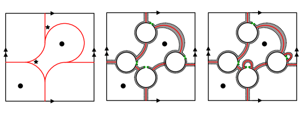
Figure 13. Arc diagrams from train tracks. Left: a train track on a twice-punctured torus. Center: the corresponding arc diagram $\mathcal{Z}$ from Construction 7.1. The cores of the handles ($\alpha$-arcs in an associated Heegaard diagram) are solid, the surface $F(\mathcal{Z})$ is shaded, the intervals $S_{-}$ on its boundary are dotted, and the sutures $\partial S_{+}=\partial S_{-}$ are indicated with small circles. Right: the arc diagram $\mathcal{Z}_{\sigma}$ from Construction 7.3, where $\sigma$ chooses the two cusps marked with stars.

Construction 7.1.

Let $\tau$ be a generic, filling train track on $\Sigma$. Associated to $\tau$ one can construct an arc diagram for $\Sigma$ as follows. Let $Z^{\prime}_{i}$ be a small circle around the $i^{\text{th}}$ switch in the train track, $J_{i}$ an open interval in $Z^{\prime}_{i}$ in the cusp region, and $Z_{i}=Z^{\prime}_{i}\setminus J_{i}$. Orient each circle $Z^{\prime}_{i}$ as the boundary of a small disk around the switch, and give $Z_{i}$ the induced orientation. Let $\mathbf{a}$ be the intersection of $Z=\amalg_{i}Z_{i}$ with the train track (which is the same as the intersection of $Z^{\prime}=\amalg_{i}Z_{i}^{\prime}$ with the train track). The matching $M$ exchanges the pairs of points on the same edge of the train track. Then, for $\mathcal{Z}=(Z,\mathbf{a},M)$, the surface $F(\mathcal{Z})$ has an obvious embedding in $\Sigma$ as a neighborhood of $\tau$. The intervals $S_{+}$ are contained in small disks around the switches, while the intervals $S_{-}$ are large, in the sense that they contain the boundaries of the neighborhoods of the edges of the train track. Moreover, since $\tau$ is filling, every component of $\Sigma\setminus F(\mathcal{Z})$ is either a disk or an annulus around a component of $\partial\Sigma$. See Figure 13.

Lemma 7.2.

The arc diagram $\mathcal{Z}$ along with the embedding $F(\mathcal{Z})\hookrightarrow\Sigma$ in Construction 7.1 is, in fact, an arc diagram for $\Sigma$. That is, every component of $\partial F(\mathcal{Z})$ intersects $S_{+}$.

Proof.

Every component $K$ of $\partial F(\mathcal{Z})$ corresponds to the boundary of a component $C$ of $\Sigma\setminus\tau$, and $K$ will intersect the $S_{+}$ arcs corresponding to the cusps on the boundary of $C$. Thus, $\tau$ being a train track implies that $\mathcal{Z}$ is an arc diagram. ∎

Note that the arc diagram $\mathcal{Z}$ constructed in Construction 7.1 is not necessarily special. In fact, the number of positive (and so negative) arcs on every component of $\partial F(\mathcal{Z})$ is equal to the number of cusps on the boundary of the corresponding region of $\Sigma\setminus\tau$. We modify $\mathcal{Z}$ to a special arc diagram for $\Sigma$ as follows.

Construction 7.3.

With notation as in Construction 7.1, consider a subset $\sigma$ of the switches of $\tau$ such that if we add a star in the cusp of each switch in $\sigma$ then every component of $\Sigma\setminus\tau$ contains exactly one star. For any $i$, if the $i^{\text{th}}$ switch of $\tau$ is not in $\sigma$ then add a pair of points on $Z_{i}$ such that they bound a sub arc of $Z_{i}$ containing all three points of $Z_{i}\cap\tau$. Let $\mathbf{a}^{\prime}$ be the union of these pairs of points, and set $\mathbf{a}_{\sigma}=\mathbf{a}\cup\mathbf{a}^{\prime}$. Define the matching $M_{\sigma}$ such that it is equal to $M$ on $\mathbf{a}$ and exchanges the points of $\mathbf{a}^{\prime}$ that are on the same component of $Z$. Let $\mathcal{Z}_{\sigma}=(Z,\mathbf{a}_{\sigma},M_{\sigma})$.

For any $i$, if the $i^{\text{th}}$ switch is not in $\sigma$, then connect the switch to itself with a loop disjoint from $\tau$ and embedded in a small neighborhood of the switch in the cusp region. Denote the union of such loops by $\ell$. The surface $F(\mathcal{Z}_{\sigma})$ can be embedded into $\Sigma$ as a neighborhood of $\tau\cup\ell$. Then, $\mathcal{Z}_{\sigma}$ along with this embedding is a special arc diagram for $\Sigma$. Again, see Figure 13.

If $\Sigma$ is closed, then for any $\sigma$, the embedded sutured surface $F(\mathcal{Z}_{\sigma})$ in $\Sigma$ is isotopic to $\Sigma\setminus\amalg_{i}D_{i}$ where $D_{i}\subset\Sigma$ is the open disk neighborhood of the $i^{\text{th}}$ switch, with $\partial D_{i}=Z_{i}^{\prime}$. Under this identification, $S_{+}$ and $S_{-}$ are identified with $\amalg_{i}Z_{i}$ and $\amalg_{i}J_{i}$, respectively. If $\Sigma$ has some boundary components, some switches in $\sigma$ correspond instead to punctures of $\Sigma$ rather than extra disks which are deleted.

7.2. Arc slide sequences from periodic splitting sequences

In this section, we observe that splitting a train track (see Section 2) corresponds to performing a pair of arcslides (Definition 4.6). So, a periodic splitting sequence for a mapping class $\psi$ induces a factorization of some strongly based representative of $\psi$ into arcslides (Lemma 7.5). If we restrict to special arc diagrams, the arc diagrams before and after the sequence of arcslides may not be the same, but this can be remedied by performing a few more arcslides supported near the boundary (Corollary 7.8).

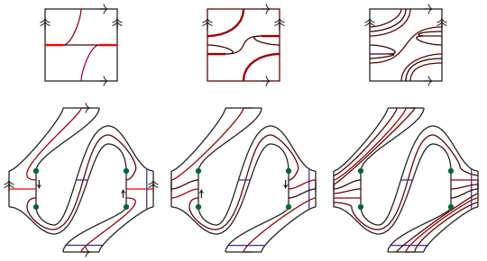
Figure 14. Trivalent train tracks and bordered-sutured Heegaard diagrams. Top: the periodic splitting sequence for the map $\tau_{a}\tau_{b}^{-1}$ on the torus. The arcs being split are thick; the splits are drawn in a particular way to correspond to the bottom row. Bottom: a corresponding sequence of arcslides starting from the half-identity diagram and ending at a half diagram for $\tau_{a}\tau_{b}^{-1}$. The dots indicate sutures and small arrows indicate where the arcslides occur.

Construction 7.4.

Suppose $\tau_{1}$ and $\tau_{2}$ are generic, filling train tracks on $\Sigma$ such that $\tau_{2}$ is obtained from $\tau_{1}$ by a split and they have the same number of branches. Let $\mathcal{Z}_{1}$ and $\mathcal{Z}_{2}$ be the arc diagrams corresponding to $\tau_{1}$ and $\tau_{2}$, respectively, from Construction 7.1. Then, as depicted in Figure 14, $\mathcal{Z}_{2}$ is obtained from $\mathcal{Z}_{1}$ by a pair of arcslides. There is an induced diffeomorphism from $F(\mathcal{Z}_{2})$ to $F(\mathcal{Z}_{1})$, and the half Heegaard diagram associated to that diffeomorphism is the result of performing these arcslides on the $\alpha$-arcs in the $\frac{\mathcal{H}}{2}(\mathit{Id}_{\mathcal{Z}_{1}})$.

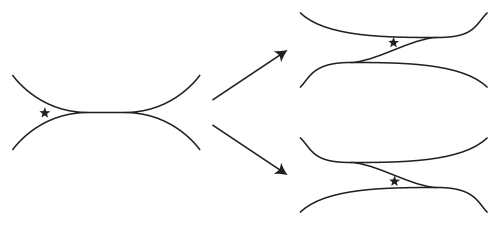
Figure 15. Induced choice of switches after a split. The switch marked with a star is one of the chosen switches, before and after the split.

Fix a subset $\sigma_{1}$ of switches in $\tau_{1}$ as in Construction 7.3. This induces a subset $\sigma_{2}$ of switches in $\tau_{2}$ such that the boundary of each component of $\Sigma\setminus\tau_{2}$ contains exactly one starred cusp (see Figure 15). (Note that the middle case of Figure 2 does not occur in the periodic splitting sequence.) Let $\mathcal{Z}_{\sigma_{1}}$ and $\mathcal{Z}_{\sigma_{2}}$ be the special arc diagrams corresponding to $\tau_{1}$ and $\tau_{2}$ as in Construction 7.3, respectively. Then $\mathcal{Z}_{\sigma_{2}}$ is obtained from $\mathcal{Z}_{\sigma_{1}}$ by the pair of arcslides corresponding to the aforementioned arcslides from $\mathcal{Z}_{1}$ to $\mathcal{Z}_{2}$.

Let $\psi$ be a pseudo-Anosov diffeomorphism of a surface $\Sigma$ and $(\tau,\mu)$ be a measured train track suited to the unstable lamination of $\psi$, from the periodic splitting sequence (Theorem 2.2). That is $(\psi(\tau),\lambda^{-1}\psi(\mu))$ is obtained from $(\tau,\mu)$ by a sequence of maximal splits. Let $\mathcal{Z}$ be the arc diagram for $\Sigma$ associated to $\tau$ by Construction 7.1. The abstract arc diagram associated to $\psi(\tau)$ by Construction 7.1 is the same as $\mathcal{Z}$. By Construction 7.4, the sequence of maximal splits from $\tau$ to $\psi(\tau)$ gives a sequence of arcslide pairs from $\mathcal{Z}$ to $\mathcal{Z}$ and so induces a strongly based diffeomorphism $\psi^{\prime}$ of $F(\mathcal{Z})$. If we let $\phi_{R}$ denote the original embedding of $F(\mathcal{Z})$, as a neighborhood of $\tau$, and $\phi_{L}$ the embedding after the arcslides, then the diffeomorphism $\psi^{\prime}$ is characterized by $\psi^{\prime}\circ\phi_{R}=\phi_{L}$. But by construction, the diffeomorphism $\psi$ also has this property (after fixing $\psi$ suitably near the boundary), so $\psi^{\prime}$ is isotopic to $\psi$ as diffeomorphisms of $\Sigma$. That is, we have proved:

Lemma 7.5.

The composition of the arcslide diffeomorphisms associated to the periodic splitting sequence for $\psi$ is a strongly based diffeomorphism which is isotopic, as a (not strongly based) diffeomorphism of $\Sigma$ to $\psi$.

Similarly, one can fix a subset $\sigma$ of the switches and construct a special arc diagram $\mathcal{Z}_{\sigma}$ for $\Sigma$ as in Construction 7.3. As we discuss in Lemma 7.7 below, the composition of the arcslides associated to the periodic splitting sequence may not give a strongly based diffeomorphism of $F(\mathcal{Z}_{\sigma})$. The following lemma will allow us to adjust the diffeomorphism near the boundary to make it strongly based, by composing with a simple sequence of arcslides.

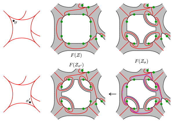
Figure 16. Diffeomorphism connecting different choices of preferred punctures. The figure shows two different choices of distinguished corner for a quadrilateral in a train track and the associated special arc diagrams. The thin arrows in the figure on the lower-right indicate a sequence of arc slides taking the arc diagram $F(\mathcal{Z}_{\sigma})$ to $F(\mathcal{Z}_{\sigma^{\prime}})$ (up to isotopy).

Lemma 7.6.

Let $\sigma_{1}$ and $\sigma_{2}$ be two subsets of the cusps of $\tau$ and $\mathcal{Z}_{\sigma_{1}}$ and $\mathcal{Z}_{\sigma_{2}}$ be the corresponding special arc diagrams as in Construction 7.3. There is a sequence of arcslides from $\mathcal{Z}_{\sigma_{1}}$ to $\mathcal{Z}_{\sigma_{2}}$ such that the points corresponding to the sub arc diagram $\mathcal{Z}$ associated to $\tau$ stay fixed. The induced diffeomorphism from $F(\mathcal{Z}_{\sigma_{2}})$ to $F(\mathcal{Z}_{\sigma_{1}})$ extends to a diffeomorphism of $\Sigma$ which is isotopic to the identity.

Proof.

Each positive arc (component of $S_{+}$) in $\partial F(\mathcal{Z})$ corresponds to a switch in $\tau$. So, a choice of subset $\sigma$ specifies a subset of positive arcs that includes exactly one positive arc on each component of $\partial F(\mathcal{Z})$. The sutured surface $F(\mathcal{Z}_{\sigma})$ is obtained from $F(\mathcal{Z})$ by attaching a $1$-handle to $S_{-}$ for each component of $S_{+}$ that is not associated to a switch in $\sigma$. (See Figure 16.) Consider a component of $\partial F(\mathcal{Z})$ on which $\sigma_{1}$ and $\sigma_{2}$ specify distinct positive arcs. In the construction of $F(\mathcal{Z}_{\sigma_{1}})$, a $1$-handle has been attached to $\partial F(\mathcal{Z})$ at the switch distinguished by $\sigma_{2}$ (since by assumption $\sigma_{1}$ does not choose this arc). Sliding the feet of this $1$-handle as in Figure 16 gives a $1$-handle attached to $\partial F(\mathcal{Z})$ corresponding to the arc distinguished by $\sigma_{1}$. This specifies a sequence of arcslides from $F(\mathcal{Z}_{\sigma_{1}})$ to $F(\mathcal{Z}_{\sigma_{1}^{\prime}})$ where $\sigma_{1}^{\prime}$ coincides with $\sigma_{2}$ on the boundary component of $F(\mathcal{Z})$ under consideration and coincides with $\sigma_{1}$ on other components. Repeating this process gives a sequence of arcslides from $F(\mathcal{Z}_{\sigma_{1}})$ to $F(\mathcal{Z}_{\sigma_{2}})$. Since the induced diffeomorphism from $F(\mathcal{Z}_{\sigma_{2}})$ to $F(\mathcal{Z}_{\sigma_{1}})$ is equal to identity on the subsurface $F(\mathcal{Z})\setminus\mathrm{nbd}(\partial F(\mathcal{Z}))$, the extension of this diffeomorphism on $\Sigma$ is isotopic to identity. ∎

As discussed in the proof of Lemma 2.3, the diffeomorphism $\psi$ induces a correspondence between the cusps on the boundaries of the complementary regions of $\tau$. So, any subset $\sigma$ will get mapped to another subset, denoted by $\psi(\sigma)$.

Lemma 7.7.

Let $\sigma$ be a subset of switches as in Construction 7.3. The sequence of maximal splits from $\tau$ to $\psi(\tau)$ induces a sequence of arcslides from $\mathcal{Z}_{\sigma}$ to $\mathcal{Z}_{\psi^{-1}(\sigma)}$. The strongly based diffeomorphism represented by the composition of these arcslides extends to a diffeomorphism of $\Sigma$ representing the mapping class of $\psi$.

Proof.

Let $\mathcal{Z}$ be the arc diagram associated to $\tau$. As in the proof of Lemma 7.6, each positive arc in $\partial F(\mathcal{Z})$ corresponds to a switch and so a cusp on the boundary of a complementary region of $\tau$. The sequence of arcslide pairs associated to the maximal split induces a strongly based diffeomorphism on $F(\mathcal{Z})$ such that its restriction to $S_{+}$, under the identification with cusps, is equal to the induced map by $\psi$. Therefore, the result of the arcslide moves on $\mathcal{Z}_{\sigma}$ is $\mathcal{Z}_{\psi^{-1}(\sigma)}$ and the induced diffeomorphism from $F(\mathcal{Z}_{\psi^{-1}(\sigma)})$ to $F(\mathcal{Z}_{\sigma})$ extends to a diffeomorphism isotopic to $\psi$ on $\Sigma$. ∎

Corollary 7.8.

For any subset $\sigma$ of switches as in Construction 7.3, the composition of the arcslide diffeomorphism from $F(\mathcal{Z}_{\sigma})$ to $F(\mathcal{Z}_{\psi^{-1}(\sigma)})$ as in Lemma 7.6 and the arcslide diffeomorphism associated to maximal splits from $F(\mathcal{Z}_{\psi^{-1}(\sigma)})$ to $F(\mathcal{Z}_{\sigma})$ as in Lemma 7.7 is a strongly based diffeomorphism from $F(\mathcal{Z}_{\sigma})$ to $F(\mathcal{Z}_{\sigma})$ that extends to a diffeomorphism isotopic to $\psi$ on $\Sigma$.

8. Compressing surface diffeomorphisms

The goal of this section is to prove Theorem 1.5 (restated as Theorem 8.15, below), that bordered-sutured Floer homology detects when a mapping class $\phi$ extends over some compression body and, in particular, that there is an explicit bound on the number of generators of the bordered-sutured module involved. The general strategy of the proof is similar to Casson-Long’s proof that there is an algorithm to determine whether a diffeomorphism extends over some compression body (and, in fact, we use some of their results). The main difference is that their bounds are in terms of lengths of geodesics with respect to some hyperbolic metric, while we need bounds adapted to Heegaard diagrams. So, Sections 8.1 and 8.2 give analogues of some of their results in terms of the number of intersections of curves with the triangulation dual to a train track. Section 8.1 focuses on the lengths of curves, while Section 8.2 constructs compression bodies represented by bases of bounded length. Section 8.3 then uses the bounded-length compression bodies to build a particular Heegaard diagram in which we can understand the number of intersection points, proving Theorem 1.5. Unlike in the previous section, we require $\psi$ to be a diffeomorphism of a closed surface here; this is needed for the proof of Lemma 8.7.

Notation 8.1.

Given a pseudo-Anosov diffeomorphism $\psi$ of a closed surface $\Sigma$, let:

• $\tau$ be a train track, suited to the unstable foliation of $\psi$, from the periodic splitting sequence (so repeatedly applying maximal splits to $\tau$ eventually gives $\psi(\tau)$),

• $\mathcal{T}$ be the triangulation of $\Sigma$ dual to $\tau$,

• $v(\mathcal{T})$ denote the set of vertices of $\mathcal{T}$,

• $s$ denote the number of switches of $\tau$,

• $l$ denote the number of edges of $\tau$, and

• $\kappa=|v(\mathcal{T})|$ denote the number of connected components of $\Sigma\setminus\tau$.

8.1. Discrete length via triangulation

In this section, we use the triangulation $\mathcal{T}$ to define a notion of length for curves in $\Sigma$, and then study how the length grows when one applies $\psi$, as well as the number of intersections between a curve and its image under $\psi$.

For any simple closed curve $\gamma\subset\Sigma$, let $\ell(\gamma)=\imath(\gamma,\mathcal{T})$ be the geometric intersection number of $\gamma$ with the edges of $\mathcal{T}$, that is, the minimum number of times that a simple closed curve $\gamma^{\prime}\subset\Sigma\setminus v(\mathcal{T})$ isotopic to $\gamma$ in $\Sigma$ intersects $\mathcal{T}$.

Recall from Section 3 that a basis for a compression body $C$ is a collection of curves in $\Sigma$ specifying $C$. Let $B(C)$ denote the set of all bases for $C$, and define

(8.2) $$\ell(C)=\min_{\left\{\gamma_{1},\dots,\gamma_{n}\right\}\in B(C)}\sum_{i=1}^{n}\ell(\gamma_{i}).$$

We pause to show that for $\gamma=\cup_{i=1}^{n}\gamma_{i}$, the minimal length of an embedded representative of $\gamma$ is equal to $\ell(\gamma)=\sum_{i=1}^{n}\ell(\gamma_{i})$. Certainly $\sum\ell(\gamma_{i})$ is a lower bound for the length of an embedded representative for $\gamma$. Conversely, suppose $\gamma^{\prime}_{i}$ is a minimal-length representative of $\gamma_{i}$ and $\gamma^{\prime}=\cup_{i=1}^{n}\gamma^{\prime}_{i}$. The curve $\gamma^{\prime}$ may be immersed rather than embedded, but is regularly homotopic to $\gamma$. Hence, $\gamma^{\prime}$ can be made embedded by a sequence of isotopies supported in bigons on $\Sigma$ with boundary on $\gamma^{\prime}$ and interior disjoint from $\gamma^{\prime}$. Since $\#(\gamma^{\prime}\cap\mathcal{T})=\ell(\gamma)$, both sides of each bigon intersect $\mathcal{T}$ in the same number of points, so such isotopies do not change $\#(\gamma^{\prime}\cap\mathcal{T})$.

Since $\tau$ is from the periodic splitting sequence, $\psi(\tau)$ is obtained from $\tau$ by a sequence of maximal splits. So, $\psi(\tau)$ is carried by $\tau$ with carrying map induced by the splitting sequence. Denote the associated incidence matrix by $M=(m_{ij})$.

We assume $\psi(\tau)$ intersects $\tau$ transversely. Denote the $l$ branches of $\tau$ by $b_{1},b_{2},\dots,b_{l}$. By isotoping $\psi$ in a neighborhood of $\tau$, we can arrange that for any branches $b_{i}$ and $b_{j}$, $\psi(b_{j})\cap b_{i}$ consists of at most $m_{ij}$ points.

Let

(8.3) $$r(\psi)=\max_{j}\left\{\sum_{i=1}^{l}m_{ij}\right\}.$$

That is, $r(\psi)$ is the largest entry of $(1,\dots,1)M$.

Lemma 8.4.

For any simple closed curve $\gamma$ on $\Sigma$ we have

$$\ell(\psi(\gamma))\leq r(\psi)\ell(\gamma).$$

Proof.

Consider a representative of $\gamma$ in a small tubular neighborhood $\mathrm{nbd}(\tau)$ of $\tau$ such that $\gamma$ intersects $\mathcal{T}$ in $\imath(\gamma,\mathcal{T})$ points. Any representative of $\gamma$ with minimal length can be isotoped into $\mathrm{nbd}(\tau)$ (not necessarily carried by $\tau$), so such a representative exists. Let

$$V_{\gamma}=\left(\#(T_{1}\cap\gamma),\dots,\#(T_{l}\cap\gamma)\right)^{T},$$

where $T_{i}$ denotes the edge of $\mathcal{T}$ dual to the branch $b_{i}$ of $\tau$. Then $\psi(\gamma)$ has a representative in $\mathrm{nbd}(\tau)$ so that its intersections with the edges of $\mathcal{T}$ are given by the entries of the vector $MV_{\gamma}$. This representative does not necessarily have minimal geometric intersection number with $\mathcal{T}$, but this still gives

$$\ell(\psi(\gamma))\leq(1,1,\dots,1)MV_{\gamma}\leq r(\psi)\ell(\gamma),$$

as desired. ∎

Lemma 8.5.

For any simple closed curve $\gamma$ on $\Sigma$, we have

$$\imath(\gamma,\psi(\gamma))\leq r(\psi)\left(\ell(\gamma)\right)^{2}$$

Proof.

As in the proof of Lemma 8.4, consider a representative of $\gamma$ in a small neighborhood of $\tau$ such that $\gamma$ intersects $\mathcal{T}$ in $\imath(\mathcal{T},\gamma)$ points, and let $V_{\gamma}=(v_{1},v_{2},\dots,v_{l})^{T}$ be the corresponding vector, so $v_{i}=\#(\gamma\cap T_{i})$. Then $\psi(\gamma)$ has a representative in a sufficiently small neighborhood of $\psi(\tau)$ such that $\#(\psi(\gamma)\cap b_{i})\leq\#(\psi(\gamma)\cap T_{i})=\sum_{j=1}^{l}m_{ij}v_{j}$. So, for a representative of $\gamma$ in a sufficiently small neighborhood of $\tau$ so that $\gamma$ goes over the branch $b_{i}$ $v_{i}$-many times, each intersection point of $\psi(\gamma)$ with $b_{i}$ will result in $v_{i}$ intersection points in $\gamma\cap\psi(\gamma)$, and thus we have

$$\#\left(\gamma\cap\psi(\gamma)\right)\leq V_{\gamma}^{T}MV_{\gamma}\leq|V_{\gamma}||MV_{\gamma}|\leq\ell(\gamma)\left((1,1,\dots,1)MV_{\gamma}\right)\leq r(\psi)\left(\ell(\gamma)\right)^{2},$$

as desired. ∎

8.2. Existence of a compression with bounded complexity

In this section, we prove that if $\psi$ extends over some compression body, it will extend over a compression body $C$ for which $\ell(C)$ is bounded above by a specific constant defined in terms of $\psi$ and $\tau$ (See Lemma 8.10).

The incidence matrix $M$ for the carrying $\psi(\tau)<\tau$ is a non-negative Perron-Frobenius matrix, and so for sufficiently large $k$ all entries of $M^{k}$ are positive. Let $K>0$ be the smallest number such that for any $k\geq K$, $M^{k}$ is positive and write $M^{K}=\left(n_{ij}\right)$.

Consider a maximal diagonal extension $\widetilde{\tau}$ of $\tau$. By Lemma 2.3, there is a maximal diagonal extension $\widetilde{\tau}^{\prime}$ of $\tau$ that carries $\psi^{K}(\widetilde{\tau})$, $\psi^{K}(\widetilde{\tau})<\widetilde{\tau}^{\prime}$ and the carrying map extends the carrying $\psi^{K}(\tau)<\tau$. For each maximal diagonal extension $\widetilde{\tau}$ fix a $\widetilde{\tau}^{\prime}$ with these properties. Let $N_{\widetilde{\tau}}=(\widetilde{n}_{ij})$ be the corresponding incidence matrix and define

$$c(N_{\widetilde{\tau}})=2\max_{i}\left\{\sum_{j=1}^{\widetilde{l}}\widetilde{n}_{ij}\right\}+1,\quad\quad\quad c(\psi)=\max_{\widetilde{\tau}}\left\{c(N_{\widetilde{\tau}})\right\}.$$

Here, $\widetilde{l}$ denotes the number of branches in $\widetilde{\tau}$, and in the definition of $c(\psi)$ we take the maximum over all maximal diagonal extensions $\widetilde{\tau}$ of $\tau$ (where for each $\widetilde{\tau}$ we choose some $\widetilde{\tau}^{\prime}$).

Moreover, for any diagonal $d$ of $\tau$ let $\ell(d)$ be the minimum over arcs $d^{\prime}$ isotopic to $d$ rel endpoints of the number of times that $d^{\prime}$ intersects the dual triangulation $\mathcal{T}$. Define

$$c^{\prime}(\psi)=\max\{\ell(d)\mid d\text{ is a diagonal of }\tau\}.$$

Lemma 8.6.

Let $\gamma\subset\Sigma$ be a simple closed curve. For any sufficiently large $n$, there exists a maximal diagonal extension $\widetilde{\tau}$ of $\tau$ such that

1. $\psi^{n}(\gamma)$ is carried by $\widetilde{\tau}$

2. for any subarc $\alpha$ of $\psi^{n}(\gamma)$, if the image of $\alpha$ under the carrying map goes over at least $c(\psi)$ branches of $\widetilde{\tau}$, then $\alpha$ goes over every branch of $\tau\subset\widetilde{\tau}$.

Proof.

The sequence $\{\psi^{n}(\gamma)\}$ converges to the unstable foliation of $\psi$ in $\mathcal{PML}(\Sigma)$. By Lemma 2.1, there exists an $N>0$ such that for any $n\geq N$ the curve $\psi^{n}(\gamma)$ is carried by some maximal diagonal extension $\widetilde{\tau}_{n}$ of the train track $\tau$. Note that $\widetilde{\tau}_{n}$ might depend on $n$. Let $\widetilde{\tau}_{n}^{\prime}$ be the fixed maximal diagonal extension of $\tau$ that carries $\psi^{K}(\widetilde{\tau}_{n})$ with a carrying map that extends the carrying $\psi^{K}(\tau)<\tau$ as above. The carrying map for $\psi^{K}(\widetilde{\tau}_{n})<\widetilde{\tau}_{n}^{\prime}$ gives a carrying of $\psi^{n+K}(\gamma)$ by $\widetilde{\tau}_{n}^{\prime}$. Suppose $\alpha$ is a subarc of $\psi^{n+K}(\gamma)$ so that the image of $\alpha$ under the carrying map goes over $c(\psi)$ branches of $\widetilde{\tau}_{n}^{\prime}$. The definition of $c(\psi)$ implies that the image of $\alpha$ under the carrying map contains the image of $\psi^{K}(b)$ under the carrying map for some branch $b\subset\tau$. On the other hand, $M^{K}$ has strictly positive entries, so for every branch $b$ of $\tau$ the image of $\psi^{K}(b)$ under the carrying map $\psi^{K}(\tau)<\tau$ goes over every branch of $\tau$. Therefore, the claim holds for any $n\geq N+K$ with $\widetilde{\tau}=\widetilde{\tau}_{n-K}^{\prime}$ along with the described carrying map. ∎

Lemma 8.7.

Suppose $\psi$ extends over some compression body $C$ with $\partial C=\Sigma$. Then there exists an essential simple closed curve $\gamma\subset\Sigma$ such that $\ell(\gamma)\leq c(\psi)+c^{\prime}(\psi)$ and $\gamma$ bounds a disk in $C$.

Proof.

The proof is similar to the proof of [CL85, Theorem 1.2]. Let $\gamma\subset\Sigma$ be an essential simple closed curve that bounds a disk in $C$. As $n$ goes to infinity, $\psi^{-n}(\gamma)$ converges to the stable foliation of $\psi$ in $\mathcal{PML}(\Sigma)$. So, by Lemma 2.4, for $n\gg 0$, $\psi^{-n}(\gamma)$ is carried by some maximal diagonal extension $\widetilde{\tau}^{*}$ of the dual bigon track $\tau^{*}$. Thus, choose $n$ large enough so that:

1. By Lemma 8.6, $\psi^{n}(\gamma)$ is isotopic to a simple closed curve $\gamma_{n}$ so that $\gamma_{n}$ is contained in a small fibered neighborhood $\mathrm{nbd}(\widetilde{\tau})$ of some maximal diagonal extension $\widetilde{\tau}$ of $\tau$, is carried by $\widetilde{\tau}$, and any subarc of $\gamma_{n}$ that goes over $c(\psi)$ branches of $\widetilde{\tau}$ goes over every branch of $\tau$.

2. $\psi^{-n}(\gamma)$ is isotopic to an essential simple closed curve $\gamma_{-n}$ in a small fibered neighborhood $\mathrm{nbd}(\widetilde{\tau}^{*})$ of some maximal diagonal extension $\widetilde{\tau}^{*}$ of the dual bigon track $\tau^{*}$ and $\psi^{-n}(\gamma)$ is carried by $\widetilde{\tau}^{*}$.

Choose the neighborhoods $\mathrm{nbd}(\widetilde{\tau})$ and $\mathrm{nbd}(\widetilde{\tau}^{*})$ small enough that the intersection points of $\gamma_{n}$ and $\gamma_{-n}$ correspond to the intersection points of $\widetilde{\tau}$ and $\widetilde{\tau}^{*}$. Since $\psi$ extends over $C$, both $\gamma_{n}$ and $\gamma_{-n}$ bound properly embedded disks in $C$, which we denote $D$ and $D^{\prime}$, respectively. We assume that $D$ and $D^{\prime}$ intersect transversely, and we remove circle components of $D\cap D^{\prime}$ by isotopy. So, $D\cap D^{\prime}$ is a disjoint union of properly embedded arcs. Define a pairing $\sim$ on the intersection points $\gamma_{n}\cap\gamma_{-n}$ by setting $x\sim y$ if there exists an arc $\eta$ in $D\cap D^{\prime}$ so that $\partial\eta=\{x,y\}$.

Choose an arc $\alpha\subset\gamma_{n}$ satisfying the following:

1. for any $x,y\in\gamma_{n}\cap\gamma_{-n}$, if $x\sim y$ then $x\in\alpha$ if and only if $y\in\alpha$,

2. $\alpha$ goes over at least $c(\psi)$ branches of $\widetilde{\tau}$, and

3. $\alpha$ is minimal with respect to conditions (1) and (2), i.e., there is no subarc of $\alpha$ satisfying (1) and (2).

(See Figure 17.)

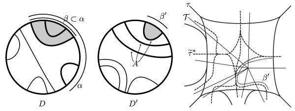
Figure 17. Bounding the length of a curve that bounds a disk. Left and center: the disks $D$ and $D^{\prime}$. The new disk $C\subset D\cup D^{\prime}$ is shaded. The arcs in $A$ are thick. Right: part of the train tracks $\tau$ (solid) and $\widetilde{\tau}^{*}$ (dashed), the dual triangulation (thin) $\mathcal{T}$, and the curve $\beta^{\prime}$ (dotted). The contribution of this region to $c^{\prime}(\psi)$ is $4$ (via the diagonal from the top-left to the bottom-right). Since the curve $\beta^{\prime}$ shown intersects $\mathcal{T}$ in this region five points, it is straightened to an arc intersecting $\mathcal{T}$ in one point, instead.

Consider the subset $A$ of $D\cap D^{\prime}$ consisting of the arcs whose boundary is in $\alpha$. An innermost arc of $A\subset D^{\prime}$ decomposes $\partial D^{\prime}=\gamma_{-n}$ into two arcs so that the interior of one of them, denoted $\beta^{\prime}$, is disjoint from $\alpha$. Since the interior of $\beta^{\prime}$ is disjoint from $\alpha$, which goes over every branch of $\tau$, $\beta^{\prime}$ is in one region of $\Sigma\setminus\tau$. Moreover, $\beta^{\prime}$ is carried by $\widetilde{\tau}^{*}$, so $\beta^{\prime}$ can be modified by an isotopy that fixes its end points and is supported in exactly one region of $\Sigma\setminus\tau$ so that $\#(\beta^{\prime}\cap\mathcal{T})\leq c^{\prime}(\psi)$.

Let $\beta$ be the subarc of $\alpha$ with $\partial\beta=\partial\beta^{\prime}$. This arc satisfies (1) and so minimality of $\alpha$ implies that the number of intersection points in $\beta\cap\mathcal{T}$ is less than or equal to $c(\psi)$. (Equality holds when $\beta=\alpha$.) Let $\gamma=\beta\cup\beta^{\prime}$. It is easy to see that $\gamma$ bounds a disk in $C$.

The dual bigon track for the train track $\widetilde{\tau}$ is obtained by collapsing $\tau^{*}$ along admissible arcs, as in Figure 7. Splitting this dual bigon track at the large branches associated to these collapses results in a (combed) maximal diagonal extensions of $\tau^{*}$. From the proof of Lemma 2.4, we may assume that $\widetilde{\tau}^{*}$ is one of the maximal diagonal extensions obtained this way. Since $\widetilde{\tau}$ intersects its dual efficiently, it intersects $\widetilde{\tau}^{*}$ efficiently as well. Thus, $\gamma$ is an essential curve in $\Sigma$. Moreover, $\ell(\beta\cup\beta^{\prime})\leq c(\psi)+c^{\prime}(\psi)$, so we are done. ∎

Definition 8.8.

Given an embedded $1$-dimensional submanifold $\gamma$ in $\Sigma$ consisting of essential simple closed curves, and a compression body $C$ with outer boundary $\Sigma$, we say $\gamma$ compresses in $C$ if every connected component of $\gamma$ bounds a disk in $C$.

Given two 1-dimensional submanifolds $\gamma$ and $\gamma^{\prime}$ of $\Sigma$, Casson and Long [CL85, Lemma 2.2] construct a finite (possibly empty) collection of compression bodies $B(\gamma,\gamma^{\prime})=\{C_{1},\dots,C_{n}\}$ satisfying the following:

1. For every $i$, each curve in $\gamma$ or $\gamma^{\prime}$ bounds a disk in $C_{i}$.

2. If every closed curve in $\gamma$ or $\gamma^{\prime}$ bounds a disk in some compression body $C$, then some $C_{i}\subseteq C$.

3. The set $B(\gamma,\gamma^{\prime})$ is minimal with respect to the properties (1) and (2), i.e., no proper subset of $B(\gamma,\gamma^{\prime})$ satisfies both properties.

We recall the construction of $B(\gamma,\gamma^{\prime})$. Suppose $\gamma=\coprod_{i=1}^{k}\gamma_{i}$ and $\gamma^{\prime}=\coprod_{j=1}^{l}\gamma^{\prime}_{j}$ where each $\gamma_{i}$ and $\gamma^{\prime}_{j}$ is an essential simple closed curve. Suppose there exists some compression body $C$ such that every $\gamma_{i}$ and $\gamma_{j}^{\prime}$ bounds a disk in $C$ otherwise, $B(\gamma,\gamma^{\prime})=\emptyset$. Let $D=\coprod_{i=1}^{k}D_{i}$ and $D^{\prime}=\coprod_{j=1}^{l}D^{\prime}_{j}$ be disjoint unions of properly embedded disks in $C$ so that $\partial D_{i}=\gamma_{i}$, $\partial D^{\prime}_{j}=\gamma^{\prime}_{j}$ and $D_{i}$ intersects $D^{\prime}_{j}$ in a set of pairwise disjoint arcs for any $i$ and $j$. Then $D\cap D^{\prime}$ induces a pairing on $\gamma\cap\gamma^{\prime}$ by setting $x\sim y$ if and only if $\{x,y\}$ is the boundary of an arc in $D\cap D^{\prime}$. Clearly, this pairing has the following properties:

• if $x\sim y$ then $x$ and $y$ lie on the same connected components of $\gamma$ and $\gamma^{\prime}$

• for any subarc $\alpha$ in $\gamma$ or $\gamma^{\prime}$ where $\partial\alpha$ consists of paired points, and any pair $x\sim y$, either $\{x,y\}\cap\mathrm{int}(\alpha)=\emptyset$ or $\{x,y\}\cap\mathrm{int}(\alpha)=\{x,y\}$.

On the other hand, given any pairing on the intersection points $\gamma\cap\gamma^{\prime}$ satisfying the above properties, one can construct a compression body that both $\gamma$ and $\gamma^{\prime}$ compress in, as follows. Consider paired points $x\sim y$ on $\gamma$ such that there exists an arc $\alpha\subset\gamma$ with $\partial\alpha=\{x,y\}$ and $\mathrm{int}(\alpha)\cap\gamma^{\prime}=\emptyset$. Let $\gamma^{\prime}_{j}$ be the component of $\gamma^{\prime}$ containing $x$ and $y$. Modify $\gamma^{\prime}$ and remove the pair of intersection points $\{x,y\}\subset\gamma\cap\gamma^{\prime}$ by doing surgery on $\gamma^{\prime}_{j}$ at $x$ and $y$ along $\alpha$. One can remove all of the intersections points between $\gamma$ and $\gamma^{\prime}$ by repeating this process. The resulting set of pairwise disjoint simple closed curves defines a compression body that every component of $\gamma$ or $\gamma^{\prime}$ bounds a disk in. Moreover, if both $\gamma$ and $\gamma^{\prime}$ compress in some compression body $C$, then $C$ contains the compression body associated to the pairing induced by $C$ on $\gamma\cap\gamma^{\prime}$. Then $B(\gamma,\gamma^{\prime})$ will be a subset of the finite set of compression bodies corresponding to these pairings. To make the set $B(\gamma,\gamma^{\prime})$ minimal, if the compression body associated to one pairing is contained in the compression body associated to another then one drops the larger of the two. (Checking if one compression body is contained in another can be done using the fundamental group, say, or using twisted Floer homology, to check if the curves in a basis for the smaller compression body bound disks in the bigger compression body.)

Lemma 8.9.

Assume $\gamma$ and $\gamma^{\prime}$ are embedded $1$-manifolds consisting of essential circles on $\Sigma$ and $B(\gamma,\gamma^{\prime})\neq\emptyset$. Then for any $C_{i}\in B(\gamma,\gamma^{\prime})$ we have

$$\ell(C_{i})\leq\ell(\gamma)+\ell(\gamma^{\prime})+\imath(\gamma,\gamma^{\prime})\min\{\ell(\gamma),\ell(\gamma^{\prime})\}.$$

Proof.

Suppose $\gamma$ and $\gamma^{\prime}$ intersect $\mathcal{T}$ minimally, i.e., in $\ell(\gamma)$ and $\ell(\gamma^{\prime})$ points, respectively. If $\#(\gamma\cap\gamma^{\prime})>\imath(\gamma,\gamma^{\prime})$ there exists an embedded bigon on $\Sigma$ whose interior is disjoint from $\gamma\cup\gamma^{\prime}$ and whose boundary consists of an arc on $\gamma$ and an arc on $\gamma^{\prime}$. Since $\gamma$ and $\gamma^{\prime}$ intersect $\mathcal{T}$ minimally, both arcs on the boundary of this bigon intersect $\mathcal{T}$ in the same number of points, and so modifying $\gamma^{\prime}$ with an isotopy supported in a small neighborhood of this bigon to remove the corresponding pair of intersection points does not change $\#(\gamma^{\prime}\cap\mathcal{T})$. Repeating this process, we get representatives of $\gamma$ and $\gamma^{\prime}$ that intersect $\mathcal{T}$ minimally and satisfy $\#(\gamma\cap\gamma^{\prime})=\imath(\gamma,\gamma^{\prime})$.

Suppose $\ell(\gamma)\leq\ell(\gamma^{\prime})$. Then given a pairing on $\gamma\cap\gamma^{\prime}$, each step of removing a pair of intersection points by modifying $\gamma^{\prime}$ will add at most $2\ell(\gamma)$ to the total number of intersection points between the curves and the edges of the ideal triangulation $\mathcal{T}$. If $\ell(\gamma)\geq\ell(\gamma^{\prime})$ we can remove the intersection points by modifying $\gamma$ instead of $\gamma^{\prime}$. So, we are done. ∎

Lemma 8.10.

If $\psi$ extends over some compression body, then it extends over a compression body $C$ with

$$\ell(C)\leq(\overbrace{F_{\psi}\circ\cdots\circ F_{\psi}}^{2g})\left(c(\psi)+c^{\prime}(\psi)\right)$$

where $F_{\psi}(x)=(1+r(\psi))x+r(\psi)x^{3}$.

Proof.

Let $C^{\prime}$ be a compression body that $\psi$ extends over. By Lemma 8.7, there exists an essential simple closed curve $\gamma$ that compresses in $C^{\prime}$ with $\ell(\gamma)\leq c(\psi)+c^{\prime}(\psi)$. We construct a rooted tree, such that each vertex corresponds to a set of pairwise disjoint essential curves on $\Sigma$, $\gamma$ is the root, and the children of each vertex $\gamma^{\prime}$ are in one-to-one correspondence with compression bodies in $B(\gamma^{\prime},\psi(\gamma^{\prime}))$, unless $B(\gamma^{\prime},\psi(\gamma^{\prime}))$ has one element. (Cf. [CL85, Proof of Theorem 2.1].) Specifically, if $B(\gamma^{\prime},\psi(\gamma^{\prime}))$ has more than one element, each child of $\gamma^{\prime}$ is a basis for an element of $B(\gamma^{\prime},\psi(\gamma^{\prime}))$ achieving the minimum in Formula (8.2) (i.e., a minimal length basis). If $B(\gamma^{\prime},\psi(\gamma^{\prime}))$ has one element (i.e., $\psi$ extends over $\Sigma[\gamma^{\prime}]$) or $B(\gamma^{\prime},\psi(\gamma^{\prime}))=\emptyset$ ($\gamma^{\prime}$ and $\psi(\gamma^{\prime})$ cannot be compressed in the same compression body) then $\gamma^{\prime}$ does not have a child.

If $\gamma^{\prime\prime}$ is a child of $\gamma^{\prime}$, by Lemmas 8.9, 8.4, and 8.5, we have

$$\begin{split}\ell(\gamma^{\prime\prime})&\leq\ell(\gamma^{\prime})+\ell(\psi(\gamma^{\prime}))+\imath(\gamma^{\prime},\psi(\gamma^{\prime}))\ell(\gamma^{\prime})\\ &\leq\ell(\gamma^{\prime})+r(\psi)\ell(\gamma^{\prime})+r(\psi)\ell(\gamma^{\prime})^{3}=F_{\psi}(\ell(\gamma^{\prime})).\end{split}$$

Since $\psi$ extends over $C^{\prime}$, for some vertex $\gamma^{\prime}$ of this tree, $\psi$ extends over the compression body defined by $\gamma^{\prime}$. Let $C=\Sigma[\gamma^{\prime}]$. By [CL85, Lemma 2.3] this tree has height at most $2g$. Thus,

$$\ell(\gamma^{\prime})\leq(F_{\psi}\circ\cdots\circ F_{\psi})(\ell(\gamma))\leq(F_{\psi}\circ\cdots\circ F_{\psi})(c(\psi)+c^{\prime}(\psi)),$$

where $F_{\psi}$ is composed with itself $2g$-times. ∎

Let

(8.11) $$M(\psi):=(\overbrace{F_{\psi}\circ\cdots\circ F_{\psi}}^{2g})\left(c(\psi)+c^{\prime}(\psi)\right).$$

8.3. Special bordered-sutured diagrams and a bound on the rank of $\mathit{BSD}$

In this section, we show how to turn a train track for a diffeomorphism $\psi$ and a compression body which $\psi$ extends over into a bordered-sutured Heegaard diagram, while maintaining an explicit bound on the number of generators of the bordered module associated to the diagram. This immediately gives Theorem 1.5. The process is outlined in Figure 25.

Before turning to the construction of the Heegaard diagram, we start with two lemmas about bases for compression bodies that $\psi$ extends over.

Lemma 8.12.

Let $C$ be a compression body with outer boundary $\Sigma$. There exists an embedded, closed $1$-manifold $\gamma\subset\Sigma$ which is a basis for $C$ and satisfies the following conditions:

1. $\#(\gamma\cap\mathcal{T})=\ell(\gamma)=\ell(C)$.

2. There exist at most two intersection point of $\gamma\cap\tau$ between any two consecutive intersection points of $\gamma\cap\mathcal{T}$.

3. Every connected component of $\Sigma\setminus(\mathcal{T}\cup\gamma)$ which is a triangle with one side on $\gamma$ and two sides on $\mathcal{T}$ or a rectangle with two sides on $\gamma$ and two sides on $\mathcal{T}$ contains no switch of $\tau$.

Proof.

Let $\gamma=\coprod_{i=1}^{n}\gamma_{i}$ be a basis for $C$ such that $\gamma\pitchfork\mathcal{T}$ and $\#(\gamma\cap\mathcal{T})=\ell(\gamma)=\ell(C)$, so $\gamma$ satisfies Condition (1). Every triangle $T$ of the triangulation $\mathcal{T}$ contains exactly one switch of $\tau$. Since $\gamma$ intersects $\mathcal{T}$ minimally, $T\setminus\gamma$ consists of one special region that has nonempty intersection will all three sides of $T$, and some triangles and rectangles that intersect two sides of $T$. The curve $\gamma$ can be isotoped in the interior of $T$ such that after the isotopy the switch of $\tau$ in $T$ lies in the special region. (See Figure 18.) After doing this for every triangle of $\mathcal{T}$ we get an isotopic translate of $\gamma$ that satisfies Condition (3). Turning to Condition (2), since $\gamma$ satisfies Condition (3), if there are more than two intersection points of $\gamma\cap\tau$ between two consecutive intersection points of $\gamma\cap\mathcal{T}$ there is a bigon in the triangle $T$ containing the intersection points with boundary on $\gamma$ and $\tau$. We change $\gamma$ with a small isotopy to remove the bigon and reduce the number of intersection points. Continue this process until no such bigon is left, and the resulting $\gamma$ will satisfy Condition (2) as well. (Again, see Figure 18.) ∎

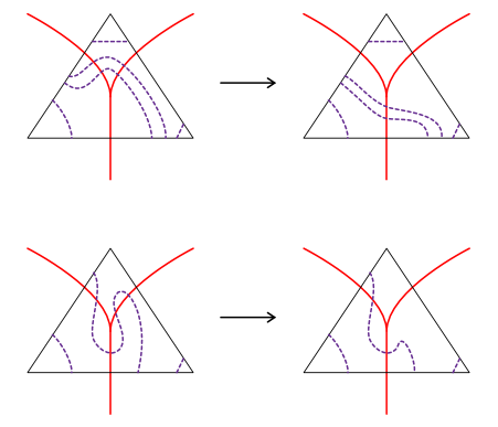
Figure 18. Local form for $\gamma$ inside a triangle. The triangle in $\mathcal{T}$ is thin, the train track $\tau$ is solid, and the 1-manifold $\gamma$ is dashed. Top: arranging that the switch lies in the unique region which is not a rectangle or triangle. Bottom: arranging that each arc of $\gamma$ intersects the train track in at most two points.

Lemma 8.13.

For any $\gamma$ satisfying the conditions of Lemma 8.12, we have $\#(\gamma\cap\tau)\leq 2\ell(\gamma)$. Moreover, every connected component of $\Sigma\setminus\gamma$ contains at least one switch of $\tau$.

Proof.

The inequality follows from condition (2). To prove the second part, if $C$ is a handlebody, then $\Sigma\setminus\gamma$ is connected and the result holds trivially. Otherwise, we define a dual graph for each connected component $A$ of $\Sigma\setminus\gamma$ as follows. Put a vertex in the interior of each connected component of $\Sigma\setminus(\mathcal{T}\cup\gamma)$ that is in $A$. If two such components share an edge that lies in $\mathcal{T}$, connect the corresponding vertices by an arc dual to this edge. If $A$ does not contain any switch of $\tau$, every component of $\Sigma\setminus(\mathcal{T}\cup\gamma)$ that is included in $A$ is either a triangle or a rectangle, and in fact $A$ is either entirely composed of triangles or entirely of rectangles. Therefore, the dual graph is a disjoint union of circles on $\Sigma$. By removing the vertices of $\mathcal{T}$ from $A$ (if $A$ is composed of triangles), we get a subset of $\Sigma$ that is homotopy equivalent to the dual graph, and so $A$ has genus $0$. However, since $\gamma$ is a basis for some compression body $C$ such that $\ell(\gamma)=\ell(C)$, every connected component of $\Sigma\setminus\gamma$ has genus strictly greater than $0$, a contradiction. ∎

Corresponding to the train track $\tau$ and any embedded $1$-manifold $\gamma\subset\Sigma$ satisfying the conditions of Lemma 8.12, we define an $(\alpha,\beta)$-bordered–sutured Heegaard diagram

$$\mathcal{H}=\left(\widetilde{\Sigma},\boldsymbol{\alpha}^{a},\boldsymbol{\beta}^{c}\cup\boldsymbol{\beta}^{a},\Gamma\right).$$

(An example is shown in Figures 25 and 26.)

First, we modify the dual graph $G=\coprod_{A}G_{A}$ defined in the proof of Lemma 8.13 to construct an embedded graph $\widetilde{G}\subset\Sigma$ whose vertices coincide with the switches of $\tau$ and so that every connected component of $\Sigma[\gamma]\setminus\widetilde{G}$ is a disk with at least three vertices (not necessarily distinct) on its boundary. (The latter condition will be needed to show the sutures can be distributed appropriately to give a bordered-sutured diagram.) For every connected component of $\Sigma\setminus(\mathcal{T}\cup\gamma)$ containing a switch of $\tau$, isotope the corresponding vertex of $G$ to coincide with the switch. The rest of the vertices of $G$ have degree two. Remove them and concatenate their adjacent edges into one edge. Every vertex in the resulting graph, which we still denote by $G$, has degree three and coincides with a switch of $\tau$. Since the inclusion of $G$ into $\Sigma\setminus(\gamma\cup v(\mathcal{T}))$ is a homotopy equivalence, each connected component of $\Sigma\setminus(\gamma\cup G)$ has one of the following types:

1. a disk containing one vertex of $\mathcal{T}$ or

2. an annulus with one boundary on $\gamma$. (The part of the boundary of the annulus along $G$ may not be embedded.)

So, $G$ divides $\Sigma[\gamma]$ into disk regions. Every type (1) region corresponds to a component of $\Sigma\setminus(\tau\cup\gamma)$ that contains a vertex of $\mathcal{T}$, as in Figure 19. For any such component, the switches on the boundary correspond to the vertices of $G$, and there is at least one switch between any two consecutive boundary arcs that lie on $\gamma$. Since every connected component of $\Sigma\setminus\tau$ contains more than one switch on the boundary, minimality of the number of intersection points between $\gamma$ and $\mathcal{T}$ implies that type (1) disk regions cannot be monogons; see Figure 20. If a type (1) disk is a bigon, then again minimality of the number of intersection points between $\gamma$ and $\mathcal{T}$ implies that its corresponding component of $\Sigma\setminus(\tau\cup\gamma)$ contains two $\gamma$ arcs on the boundary; see Figure 21. Isotoping one of these boundary arcs (and possible parallel copies) over the vertex of $\mathcal{T}$ in this component will remove this bigon, without creating a new type (1) bigon; see Figure 22.

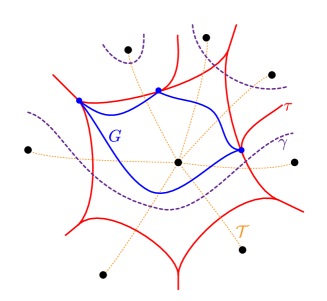
Figure 19. An example of a type (1) region. The train track $\tau$ is red, the dual triangulation $\mathcal{T}$ is thin, dashed, orange, the graph $G$ is blue, and the curves $\gamma$ are dark purple and dashed.

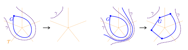
Figure 20. Nonexistence of type 1 monogons. In both figures, the existence of a type (1) monogon implies that the number of intersections of $\gamma$ and $\mathcal{T}$ can be reduced, by the indicated move. The figure on the right shows how this affects the graph $G$ in a slightly larger region; in particular, it does not introduce a new monogon. Conventions are the same as in Figure 19.

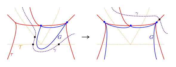
Figure 21. Nonexistence of bigons with one arc on $\gamma$. If there is a bigon with one arc on $\gamma$ then the number of intersections of $\gamma$ and $\mathcal{T}$ is not minimal. Conventions are as in Figure 19; intersections of $\gamma$ with $\mathcal{T}$ are marked with dots (as are vertices of $G$).

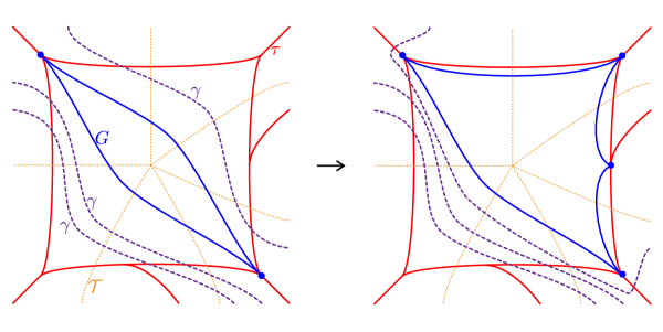
Figure 22. Removing type-1 bigons. Moving one of the arcs of $\gamma$ parallel to the bigon across the vertex eliminates the bigon. Conventions are as in Figure 19.

Next, we will remove type (2) monogons and bigons by removing edges from $G$. Let $A$ be a type (2) component. Write $\partial A=L\coprod\gamma_{A}$ where $\gamma_{A}$ is a component of $\gamma$, and $L$ is a loop in $G$. If $A$ is a monogon, so $L$ contains exactly one vertex of $G$, there exists a distinct connected component of $\Sigma\setminus(\gamma\cup G)$ that is adjacent to $A$ and contains $L$ on its boundary; denote it by $A^{\prime}$. Removing the single edge in $L$ from $G$, as in Figure 23, will result in concatenating $A$ and $A^{\prime}$, giving a disk region in $\Sigma[\gamma]$ with at least three vertices (a vertex is repeated). We repeat this until no monogons are left.

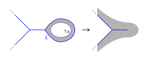
Figure 23. Removing a type (2) monogon. On the left, the annulus $A$ is shaded; $A^{\prime}$ is the unshaded region outside $A$. The picture on the right is in $\Sigma[\gamma]$, not in $\Sigma$. Removing the round edge $L$ concatenates $A$ and $A^{\prime}$; the result is still a disk in $\Sigma[\gamma]$.

Next, if $A$ is a bigon, its adjacent region(s) (regions that share an edge with $A$) are not bigons. Indeed, since vertices of $G$ either have degree three or one, if $A$ is adjacent to just one region then that region is not a bigon. Moreover, if $A$ is adjacent to a bigon then the other adjacent region must be a bigon as well. Then $\ell(\gamma)$ is not equal to $\ell(C)$, a contradiction. Thus, no two bigons are adjacent. We remove exactly one side of each bigon to make sure that none of the regions are bigons. Since no two bigons are adjacent, this process will not create a region that is not a disk. The final graph is $\widetilde{G}$.

Second, given a graph $\widetilde{G}$ as above, we use Hall’s marriage theorem to show that there exists an injective map $\sigma^{\prime}$ from $\pi_{0}(\Sigma[\gamma]\setminus\widetilde{G})$ to $v(\widetilde{G})$, where $v(\widetilde{G})$ denotes the set of vertices of $\widetilde{G}$, taking a component to a vertex on its boundary. Suppose $P_{1},P_{2},\dots,P_{m}$ are $m$ distinct components of $\Sigma[\gamma]\setminus\widetilde{G}$. Denote the number of sides in $P_{i}$ by $k_{i}$. Further, assume $\cup_{i=1}^{m}\overline{P_{i}}$ contains $v$ vertices and $e$ edges of $\widetilde{G}$. Then, since none of the $P_{i}$ are monogons or bigons,

$$3m\leq k_{1}+k_{2}+\dots+k_{m}\leq 2e\leq 3v$$

and so $v\geq m$, and therefore the claim follows from Hall’s marriage theorem.

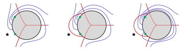
Figure 24. The form of the Heegaard diagram near the boundary. The disk $D_{i}$ is shaded; it is not part of the Heegaard diagram. The $\alpha$-arcs are solid and the $\beta$-arcs are dotted. The thin arcs indicate the intersection of the train track with $D_{i}$ and are not part of the $\alpha$-arcs. In the left figure, this switch is the switch chosen by $\sigma$ and $\sigma^{\prime}$ for the region marked $\star$. In the center, it is the switch chosen by $\sigma^{\prime}$ but not $\sigma$, so there is an extra $\alpha$-arc. On the right, this switch is not the chosen by $\sigma$ or $\sigma^{\prime}$, so there is an extra $\alpha$- and an extra $\beta$-arc.

Now, we are ready to define $\mathcal{H}$ as follows:

• Consider pairwise disjoint small disk neighborhoods $D=\coprod_{i}D_{i}$ of the switches (and so the vertices of $\widetilde{G}$) in $\Sigma\setminus\gamma$ and let $\widetilde{\Sigma}=\Sigma\setminus D$.

• On each boundary component $\partial D_{i}\subset\partial\widetilde{\Sigma}$, consider two disjoint arc sutures, both in the boundary of the cusp region of $D_{i}\cap\tau$, and let $\Gamma$ be the union of all these sutures. Let $\partial_{L}\widetilde{\Sigma}$ (respectively $\partial_{R}\widetilde{\Sigma}$) be the union of the arcs in $\partial\widetilde{\Sigma}\setminus\Gamma$ that are not disjoint (respectively are disjoint) from $\tau$. See Figure 24. Note that each component of $\partial_{L}\widetilde{\Sigma}$ intersects $\tau$ at three points.

• Let $\boldsymbol{\beta}^{c}=\gamma$.

• Let $\boldsymbol{\alpha}^{a}=\boldsymbol{\alpha}^{a,1}\coprod\boldsymbol{\alpha}^{a,2}$ where $\boldsymbol{\alpha}^{a,1}=\widetilde{\Sigma}\cap\tau$, and $\boldsymbol{\alpha}^{a,2}$ extends $\boldsymbol{\alpha}^{a,1}$ to a parameterization of the sutured surface $(\widetilde{\Sigma},\Gamma)$. Every component of $\widetilde{\Sigma}\setminus\boldsymbol{\alpha}^{a,1}$ has at least one pair of sutures on its boundary, since every region in the complement of the train track has at least one cusp. For each connected component of $\widetilde{\Sigma}\setminus\boldsymbol{\alpha}^{a,1}$ that contains more than one pair of sutures on its boundary, $\boldsymbol{\alpha}^{a,2}$ consists of arcs parallel to $\partial\widetilde{\Sigma}$ for all except one pair of these sutures, as in Figure 24. (This corresponds to making a choice $\sigma$ of one cusp for each region in the complement of the train track, as in Section 7.1.)

• Let $\boldsymbol{\beta}^{a}=\boldsymbol{\beta}^{a,1}\coprod\boldsymbol{\beta}^{a,2}$, where $\boldsymbol{\beta}^{a,1}$ is obtained as follows. The map $\sigma^{\prime}$ assigns a disk $D_{i}$, and so a boundary component of $\widetilde{\Sigma}$, to each connected component of $\widetilde{\Sigma}\setminus(\boldsymbol{\beta}^{c}\cup\widetilde{G})$. The arcs $\boldsymbol{\beta}^{a,1}$ are obtained by isotoping the arcs $\widetilde{G}\cap\widetilde{\Sigma}$ in a small neighborhood of $\partial\widetilde{\Sigma}$ so that:

  1. $\partial(\widetilde{G}\cap\widetilde{\Sigma})\subset\partial_{R}\widetilde{\Sigma}$.

  2. The sutures on the boundary components of $\widetilde{\Sigma}$ distinguished by $\sigma^{\prime}$ are on the boundary of this connected component of $\widetilde{\Sigma}\setminus(\boldsymbol{\beta}^{c}\cup\boldsymbol{\beta}^{a,1})$, as well.

  Then every connected component of $\widetilde{\Sigma}\setminus(\boldsymbol{\beta}^{c}\cup\boldsymbol{\beta}^{a,1})$ has genus zero, and contains at least one pair of sutures on its boundary.

• For any connected component of $\partial\widetilde{\Sigma}$ whose corresponding vertex is not in the image of $\sigma^{\prime}$, add a $\beta$ arc as in Figure 24 and let $\boldsymbol{\beta}^{a,2}$ be the union of these arcs.

Example 8.14.

Figure 25 shows the construction of the Heegaard diagram associated to the mapping class $\tau_{a}\tau_{b}\tau_{c}\tau_{d}^{-1}$ of a genus $2$ surface with one puncture, where $a,b,c,d$ are the curves shown, and a compression body where a single curve (passing through the edge labeled $D$ once) is being compressed. (Even though we have required surfaces to be closed in this section, except for Lemma 8.7, the construction works equally well for punctured surfaces. The train track in this example was produced by Mark Bell’s Flipper [Bel18], which gives train tracks on punctured surfaces.)

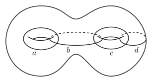
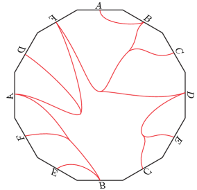
(a)	(b)
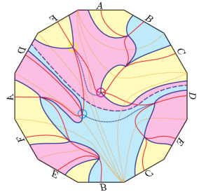
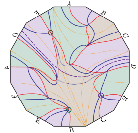
(c)	(d)

Figure 25. The Heegaard diagram associated to a train track and compression body. (a) Curves on a genus $2$ surface; the mapping class under consideration is $\tau_{a}\tau_{b}\tau_{c}\tau_{d}^{-1}$. (b) The output of Flipper applied to this mapping class. The letters indicate the edge identifications. (c) The train track, a small perturbation of Flipper’s output so that the switches are not on the polygon, is in solid red. The dual triangulation is in thin, dashed, orange. The curve $\gamma$ being compressed is purple and dashed. The graph $G^{\prime}$ is in solid blue; the graph $G$ is the union of the solid and dotted blue curves. The three components of $G\cup\gamma$ are shaded different colors. The small circles indicate a choice of vertices corresponding to these three components. (d) A coloring of the components of $\Sigma\setminus\tau$, and circles indicating a choice of components corresponding to the switches. The green region is a bigon, and contains the puncture. This figure continues as Figure 26.

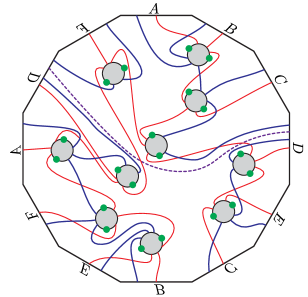
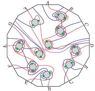
(e)	(f)

Figure 26. The Heegaard diagram associated to a train track. This is a continuation of Figure 25. (a) The Heegaard surface (complement of the shaded disks), sutures (small green circles), and the curves $\boldsymbol{\alpha}^{a,1}$ (red) $\boldsymbol{\beta}^{c}$ (purple, dashed), and $\boldsymbol{\beta}^{a,1}$ (blue). (b) The whole Heegaard diagram, including the curves $\boldsymbol{\alpha}^{a,2}$ and $\boldsymbol{\beta}^{a,2}$. There is an arc in $\boldsymbol{\beta}^{a,2}$ for each boundary component of the diagram except the three circled in Figure 25(c) and an arc in $\boldsymbol{\alpha}^{a,2}$ for each boundary component except the three circled in Figure 25(d).

Corresponding to $\mathcal{H}$, let $\mathcal{Z}_{L}$ and $\mathcal{Z}_{R}$ be the arc diagrams:

$$\begin{split}&\mathcal{Z}_{L}^{\alpha}=\left(\partial_{L}\widetilde{\Sigma},\boldsymbol{\alpha}^{a}\cap\partial_{L}\widetilde{\Sigma},M_{L}\right)\\ &\mathcal{Z}_{R}^{\beta}=\left(\partial_{R}\widetilde{\Sigma},\boldsymbol{\beta}^{a}\cap\partial_{R}\widetilde{\Sigma},M_{R}\right)\end{split}$$

where $M_{L}$ and $M_{R}$ are the matchings that pair the end points of each arc in $\boldsymbol{\alpha}^{a}$ and $\boldsymbol{\beta}^{a}$, respectively. Consider the bordered sutured Heegaard diagram $\mathcal{H}\tensor*[_{\partial_{R}}]{\cup}{{}_{\partial_{L}}}\frac{\mathcal{H}}{2}(\mathit{Id}_{\mathcal{Z}_{R}^{\beta}})$ corresponding to gluing a half-identity diagram from [LOT11, Construction 8.18] to the right boundary of $\mathcal{H}$. The bordered-sutured $3$-manifold $Y_{\mathcal{H}}$ associated to $\mathcal{H}\tensor*[_{\partial_{R}}]{\cup}{{}_{\partial_{L}}}\frac{\mathcal{H}}{2}(\mathit{Id}_{\mathcal{Z}_{R}^{\beta}})$ is obtained from the compression body $C=C_{\gamma}$ and the train track $\tau$ as follows. By definition, $C$ is constructed by attaching $2$-handles to $[0,1]\times\Sigma$ along $\{1\}\times\gamma_{i}$ for all $i$. By Lemma 8.13, every connected component of $\Sigma\setminus\gamma$ contains at least one switch of $\tau$. Let $D\subset\Sigma$ be a union of small pairwise disjoint disk neighborhoods of the switches of $\tau$ in $\Sigma$. Then, $Y_{\mathcal{H}}=C\setminus\left([0,1]\times D\right)$. The sutured part of the boundary is $[0,1]\times\partial D$ with two parallel, horizontal sutures connecting $\{0\}\times\partial D$ to $\{1\}\times\partial D$ on each connected component of $[0,1]\times\partial D$. The bordered boundary components $\{0\}\times\left(\Sigma\setminus D\right)$ and $\{1\}\times\left(\Sigma[\gamma]\setminus D\right)$ are identified with $F(\mathcal{Z}_{L}^{\alpha})$ and $F(\mathcal{Z}_{R}^{\alpha})$. As discussed in Section 4.2 the bordered-sutured manifold $Y_{\mathcal{H}}$ can be turned into a special bordered-sutured manifold by attaching $2$-handles to $\{1/2\}\times\partial D$ to get the compression body and modifying each component of $R_{+}$ and $R_{-}$ to become a bigon. This corresponds to attaching tube-cutting pieces (Figure 11) to $\mathcal{H}\tensor*[_{\partial_{R}}]{\cup}{{}_{\partial_{L}}}\frac{\mathcal{H}}{2}(\mathit{Id}_{\mathcal{Z}_{R}^{\beta}})$, one corresponding to each inner boundary component of $C$.

Theorem 8.15.

Continuing to use Notation 8.1, suppose $\psi$ extends over some compression body. Then there is a half-bordered compression body $Y$ so that $\psi$ extends over $Y$, and a way of extending the parameterization to the internal boundary of $Y$ so that the rank of $\mathit{BSD}(Y)$ is less than or equal to

(8.16) $$(20(g+s)-18)^{s}\left((2M(\psi))^{2g}+(2M(\psi)+8)^{2(g+s-1)}\right).$$

Proof.

By Lemma 8.10, there exists a compression body $C$ that $\psi$ extends over and $\ell(C)\leq M(\psi)$. Let $\gamma$ be a basis for $C$ satisfying the conditions of Lemma 8.12 and let $Y$ be the special bordered-sutured manifold corresponding to $C$, $\gamma$ and $\tau$ as described above. We will show that the number of generators in the bordered-sutured Heegaard diagram for $Y$ constructed above is bounded above by Formula (8.16).

Consider the $(\alpha,\beta)$-bordered–sutured Heegaard diagram $\mathcal{H}$ associated to $\gamma$ and $\tau$ as described above. Then the bordered-sutured Heegaard diagram for $Y$ is obtained from $\mathcal{H}\tensor*[_{\partial_{R}}]{\cup}{{}_{\partial_{L}}}\frac{\mathcal{H}}{2}(\mathit{Id}_{\mathcal{Z}_{R}^{\beta}})$ by attaching tube-cutting pieces, one for each inner boundary component of $C$.

In the Heegaard diagram $\mathcal{H}$, the number of components in $\boldsymbol{\beta}^{c}$, $\boldsymbol{\beta}^{a}$ and $\boldsymbol{\alpha}^{a}$ are equal to

$$|\boldsymbol{\alpha}^{a}|=2(g+s-1),\quad\quad|\boldsymbol{\beta}^{c}|=m,\quad\quad|\boldsymbol{\beta}^{a}|=2(g+s-m-1).$$

The total number of intersection points between $\boldsymbol{\beta}^{c}$ and $\boldsymbol{\alpha}^{a}$ is less than or equal to $2\ell(C)$, and thus $2M(\psi)$. Moreover, we may arrange for the intersection points of $\boldsymbol{\alpha}^{a}$ and $\boldsymbol{\beta}^{a}$ that are not in a neighborhood of $\partial\widetilde{\Sigma}$ to be on the $\beta$ arcs in $\boldsymbol{\beta}^{a,1}$ that correspond to the edges of $\widetilde{G}$ on the boundary of type $(2)$ annulus components of $\Sigma\setminus(\gamma\cup G)$. After fixing an orientation on the $\gamma$ curves one can define a bijection between these intersection points and the points in $\tau\cap\gamma$. So the number of such intersection points is bounded above by $2M(\psi)$. Therefore, each $\beta$ arc will have at most $2M(\psi)+8$ intersection points with $\alpha$ arcs; see Figure 24. Thus, the number of generators in $\mathcal{H}$ is bounded above by

$$(2M(\psi))^{m}+(2M(\psi)+8)^{2(g+s-m-1)}.$$

The number of generators in $\mathcal{H}$ and $\mathcal{H}\tensor*[_{\partial_{R}}]{\cup}{{}_{\partial_{L}}}\frac{\mathcal{H}}{2}(\mathit{Id}_{\mathcal{Z}_{R}^{\beta}})$ are the same, so this quantity bounds the number of generators in $\mathcal{H}\tensor*[_{\partial_{R}}]{\cup}{{}_{\partial_{L}}}\frac{\mathcal{H}}{2}(\mathit{Id}_{\mathcal{Z}_{R}^{\beta}})$, as well.

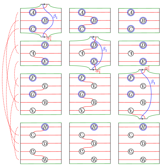
Figure 27. The tube-cutting piece. An arc diagram and three of the four associated tube-cutting pieces. There is one tube-cutting piece associated to each switch; the one not drawn is similar to the third one drawn. The two switches corresponding to the two bigons in the track have more complicated $\alpha$-circles than the two not corresponding to bigons. The arc diagram is the one from the right of Figure 13.

In each tube-cutting piece $\mathsf{TC}$, there are two kinds of generators. Each piece has a single $\alpha$-circle $\alpha_{1}^{c}$. There are $2(g+s-m-1)$ $\beta$-circles as in the identity bordered Heegaard diagram, plus one more, distinguished $\beta$-circle $\beta_{1}$. In order to make the diagram admissible, we do a finger move so that $\alpha_{1}^{c}$ and $\beta_{1}$ intersect in two points; see Figure 27. Consequently, given a generator $\mathbf{x}$ for a Heegaard diagram $\mathcal{H}$ before gluing on $\mathsf{TC}$, there are two kinds of extensions of $\mathbf{x}$ to a generator of $\mathcal{H}\cup\mathsf{TC}$: extensions using a point in $\alpha_{1}^{c}\cap\beta_{1}$ and extensions not using those points. For the former kind of extension, which $\alpha$-arcs $\mathbf{x}$ occupies completely determines which points on $\boldsymbol{\alpha}^{a}\cap\boldsymbol{\beta}$ are chosen: each $\beta$-circle is occupied on the left if the $\alpha$-arc is not occupied by $\mathbf{x}$ and on the right if the $\alpha$-arc is occupied by $\mathbf{x}$. So, $\mathbf{x}$ extends to two generators of this kind (corresponding to the two points in $\alpha_{1}^{c}\cap\beta_{1}$). For the second kind of extension, the way we have drawn the diagrams in Figure 27, which $\beta$-circles are occupied on the left is still determined, but now one of the other $\beta$-circles is occupied by a point in $\alpha_{1}^{c}$, and one of the $\alpha$-arcs on the right is occupied by a point in $\beta_{1}$. So, $\mathbf{x}$ extends to at most $20(g+s-m-1)$ generators of this kind. (We have estimated this as $5$ for the maximal number of intersection points between $\beta_{1}$ and an $\alpha$-arc times twice the number of $\beta$-arcs, for the maximum possible number of intersections of $\alpha_{1}^{c}$ with a $\beta$-arc; this is typically a gross overestimate.) Thus, the number of generators is multiplied by at most $20(g+s-m)-18$ for each tube-cutting piece. The number of tube-cutting pieces is $s$, so in all the number of generators is multiplied by

$$(20(g+s-m)-18)^{s}.$$

Therefore, the rank of $\mathit{BSD}(Y)$ is less than or equal to

$$(20(g+s-m)-18)^{s}\left((2M(\psi))^{m}+(2M(\psi)+8)^{2(g+s-m-1)}\right).$$

So, the claim follows for the fact that $m\leq 2g$. ∎

Recall that Corollary 1.6 states, somewhat imprecisely, that bordered-sutured Floer homology gives an algorithm to determine if $\psi$ extends over some compression body. We give the algorithm we have in mind as its proof:

Proof of Corollary 1.6.

First, compute the bordered-sutured bimodule associated to $\psi$ by Corollary 7.8; its description as a composition of arcslides is exactly the input to the algorithm in [LOT14] (or its easy extension to arc diagrams in [AL19]). Next, construct all bordered Heegaard diagrams for compression bodies with at most the number of generators in Formula (8.16). Compute their bordered-sutured modules, as in the proof of Corollary 6.8, and then apply Theorem 1.3 to test if $\psi$ extends over each of them. ∎

Corollary 1.6 is not quite as impractical as it might seem at first. Assume that we already know the train track $\tau$, e.g., as discussed in [Bel14]. Then Lemma 8.10 implies that $\beta$-circles in the associated Heegaard diagram intersect the triangles in the dual triangulation $\mathcal{T}$ in at most $M(\psi)$ arcs. A train track for a closed, genus $g$ surface has at most $18g-18$ edges. The number of ways to distribute the $M(\psi)$ endpoints of these arcs on the $18g-18$ edges of the triangulation is $O(M(\psi)^{18g-19})$ (as a function of $M(\psi)$; $g$ is fixed). Given the number of endpoints on each edge of a triangle, there is at most one way the edges can lie in the triangle (since the region containing the switch must be adjacent to all three sides of the triangle). So, there are at most $O(M(\psi)^{18g-19})$ choices of $\beta$-circles. Once the $\beta$-circles are fixed, the $\beta$-arcs are determined by the algorithm above. Thus, there are at most $O(M(\psi)^{18g-19})$ bordered-sutured modules to compute. In particular, the number of modules to compute is polynomial in the length $M(\psi)$.

(Of course, our bound $M(\psi)$ itself grows quickly in terms of, say, the word length of $\psi$, because $r(\psi)$ does. The time to compute the bordered-sutured modules via the algorithm in [LOT14, AL19] also seems to be exponential in the complexity of the manifold involved. One then also needs the computation of the bordered-sutured bimodule from Section 7.2, which takes exponential time in the length of the splitting sequence via the algorithm in [LOT14]. So, the algorithm is slow mostly because of the growth rate of $r(\psi)$ and the cost of computing bordered-sutured invariants.)

Theorem 8.15 gives a more algebraic obstruction to $\psi$ extending over a compression body, in that if $\psi$ extends then there must be some bordered-sutured module with at most the number of generators in Formula (8.16) and satisfying the conditions of Theorem 1.3. (Moreover, the module must look like the invariant of a handlebody in various senses, like that if one computes Formula (1.4) with $\mathit{Id}$ instead of $\psi$, the support should be $0$-dimensional.) Arguably, this is a little like saying that the bimodule $\mathit{BSDA}(\psi)$ has an eigenvector of bounded length.

References

- [ABP09] Jørgen Ellegaard Andersen, Alex James Bene, and R. C. Penner, Groupoid extensions of mapping class representations for bordered surfaces, Topology Appl. 156 (2009), no. 17, 2713–2725.
- [Ago10] Ian Agol, Ideal triangulations of pseudo-Anosov mapping tori, 2010, arXiv:1008.1606.
- [AL19] Akram Alishahi and Robert Lipshitz, Bordered Floer homology and incompressible surfaces, Ann. Inst. Fourier (Grenoble) 69 (2019), no. 4, 1525–1573.
- [Bel14] Mark C. Bell, The pseudo-Anosov and conjugacy problems are in , 2014, arXiv:1410.1358.
- [Bel18] Mark Bell, Flipper (computer software), pypi.python.org/pypi/flipper, 2013–2018.
- [BJM13] Ian Biringer, Jesse Johnson, and Yair Minsky, Extending pseudo-Anosov maps into compression bodies, J. Topol. 6 (2013), no. 4, 1019–1042.
- [BV17] Ian Biringer and Nicholas G. Vlamis, Automorphisms of the compression body graph, Journal of the London Mathematical Society 95 (2017), no. 1, 94–114, https://londmathsoc.onlinelibrary.wiley.com/doi/pdf/10.1112/jlms.12011.
- [CG83] A. J. Casson and C. McA. Gordon, A loop theorem for duality spaces and fibred ribbon knots, Invent. Math. 74 (1983), no. 1, 119–137.
- [CL85] A. J. Casson and D. D. Long, Algorithmic compression of surface automorphisms, Invent. Math. 81 (1985), no. 2, 295–303.
- [FLP79] A. Fathi, F. Laundenbach, and V. Poénaru (eds.), Travaux de Thurston sur les surfaces, Astérisque, vol. 66, Société Mathématique de France, Paris, 1979, Séminaire Orsay, with an English summary.
- [Gan59] Felix Gantmacher, Theory of matrices, Chelsea publishing, 1959.
- [Ghi08] Paolo Ghiggini, Knot Floer homology detects genus-one fibred knots, Amer. J. Math. 130 (2008), no. 5, 1151–1169.
- [GL15] Paolo Ghiggini and Paolo Lisca, Open book decompositions versus prime factorizations of closed, oriented 3-manifolds, Interactions between low-dimensional topology and mapping class groups, Geom. Topol. Monogr., vol. 19, Geom. Topol. Publ., Coventry, 2015, pp. 145–155.
- [Hak68] Wolfgang Haken, Some results on surfaces in -manifolds, Studies in Modern Topology, Math. Assoc. Amer. (distributed by Prentice-Hall, Englewood Cliffs, N.J.), 1968, pp. 39–98.
- [Han16] Jonathan Hanselman, Bordered Heegaard Floer homology and graph manifolds, Algebr. Geom. Topol. 16 (2016), no. 6, 3103–3166.
- [HLW17] Jennifer Hom, Tye Lidman, and Liam Watson, The Alexander module, Seifert forms, and categorification, J. Topol. 10 (2017), no. 1, 22–100.
- [HN10] Matthew Hedden and Yi Ni, Manifolds with small Heegaard Floer ranks, Geom. Topol. 14 (2010), no. 3, 1479–1501.
- [HN13] by same author, Khovanov module and the detection of unlinks, Geom. Topol. 17 (2013), no. 5, 3027–3076.
- [Juh06] András Juhász, Holomorphic discs and sutured manifolds, Algebr. Geom. Topol. 6 (2006), 1429–1457, arXiv:math/0601443.
- [Juh08] by same author, Floer homology and surface decompositions, Geom. Topol. 12 (2008), no. 1, 299–350, arXiv:math/0609779.
- [LOT11] Robert Lipshitz, Peter S. Ozsváth, and Dylan P. Thurston, Heegaard Floer homology as morphism spaces, Quantum Topol. 2 (2011), no. 4, 381–449, arXiv:1005.1248.
- [LOT14] by same author, Computing by factoring mapping classes, Geom. Topol. 18 (2014), no. 5, 2547–2681, arXiv:1010.2550.
- [LOT15] by same author, Bimodules in bordered Heegaard Floer homology, Geom. Topol. 19 (2015), no. 2, 525–724, arXiv:1003.0598.
- [LOT18] by same author, Bordered Heegaard Floer homology, Mem. Amer. Math. Soc. 254 (2018), no. 1216, viii+279, arXiv:0810.0687.
- [LT16] Robert Lipshitz and David Treumann, Noncommutative Hodge-to-de Rham spectral sequence and the Heegaard Floer homology of double covers, J. Eur. Math. Soc. (JEMS) 18 (2016), no. 2, 281–325.
- [Mat89] Hideyuki Matsumura, Commutative ring theory, second ed., Cambridge Studies in Advanced Mathematics, vol. 8, Cambridge University Press, Cambridge, 1989, Translated from the Japanese by M. Reid.
- [Ni07] Yi Ni, Knot Floer homology detects fibred knots, Invent. Math. 170 (2007), no. 3, 577–608.
- [Ni09] by same author, Heegaard Floer homology and fibred 3-manifolds, Amer. J. Math. 131 (2009), no. 4, 1047–1063.
- [Ni13] by same author, Nonseparating spheres and twisted Heegaard Floer homology, Algebr. Geom. Topol. 13 (2013), no. 2, 1143–1159.
- [OSz04a] Peter S. Ozsváth and Zoltán Szabó, Holomorphic disks and genus bounds, Geom. Topol. 8 (2004), 311–334.
- [OSz04b] by same author, Holomorphic disks and three-manifold invariants: properties and applications, Ann. of Math. (2) 159 (2004), no. 3, 1159–1245, arXiv:math.SG/0105202.
- [Pet18] Ina Petkova, The decategorification of bordered Heegaard Floer homology, J. Symplectic Geom. 16 (2018), no. 1, 227–277.
- [PH92] R. C. Penner and J. L. Harer, Combinatorics of train tracks, Annals of Mathematics Studies, vol. 125, Princeton University Press, Princeton, NJ, 1992.
- [PP87] Athanase Papadopoulos and Robert C. Penner, A characterization of pseudo-Anosov foliations., Pacific Journal of Mathematics 130 (1987), no. 2, 359 – 377.
- [Sta23] The Stacks Project Authors, Stacks Project, https://stacks.math.columbia.edu, 2023.
- [Wal68] Friedhelm Waldhausen, On irreducible -manifolds which are sufficiently large, Ann. of Math. (2) 87 (1968), 56–88.
- [Zar09] Rumen Zarev, Bordered Floer homology for sutured manifolds, 2009, arXiv:0908.1106.
- [Zar10] by same author, Joining and gluing sutured Floer homology, 2010, arXiv:1010.3496.
- [Zha] Bohua Zhan, bfhpython, http://github.com/bzhan/bfh_python.