High-order structure-preserving methods for damped Hamiltonian system
Abstract
We present a novel methodology for constructing arbitrarily high-order structure-preserving methods tailored for damped Hamiltonian systems. This method combines the idea of exponential integrator and energy-preserving collocation methods, effectively preserving the energy dissipation ratio introduced by the damping terms. We demonstrate the conservative properties of these methods and confirm their order of accuracy through numerical experiments involving the damped Burger’s equation and Korteweg-de-Vries equation.
keywords:
structure-preserving , damped Hamiltonian , exponential integrator , energy dissipation[inst1]organization=School of Mathematics (Zhuhai),addressline=Sun Yat-sen University, city=Zhuhai, postcode=519082, state=Guangdong, country=China
1 Introduction
In this paper, we consider damped Hamiltonian systems formulated as follows:
| (1) |
where , the matrix is skew-symmetric, the matrix is diagonal, and the energy function maps any vector to a real number. Such systems exhibit an interplay between conservative and dissipative forces. While conservative forces govern the system’s energy conservation and produce regular oscillatory behavior, damping terms introduce energy dissipation and may lead to convergence to equilibrium or other complex behaviors. These systems have become more popular in applications such as biomechanics [1] and physics [2].
It is well established that the exact solution of an Hamiltonian system without the damping term , represented by:
| (2) |
preserves the energy, i.e., , and also symplectic structure if is the canonical skew-symmetric matrix. Extensive research has focused on developing energy-preserving or symplectic numerical methods for such systems, owing to their superior numerical properties [3, 4]. When damping terms are included, the modified damped Hamiltonian system (1) preserves modified structures such as energy dissipation and conformal symplecticity, provided remains a canonical skew-symmetric matrix and and the diagonal matrix has constant equal diagonal elements [5]. Numerical methods preserving these structures include conformal symplecticity [6, 7, 8, 9, 10] and conformal multi-symplecticity [11, 12, 13, 14], as well as recently developed methods that focus on preserving correct energy dissipation rates [15, 16, 17]. Conformal symplectic methods preserve the decay rates in linear and quadratic invariants under certain constraints on the coefficient functions [10], and in general, it is not possible to design numerical methods that can preserve conformal symplecticity and energy dissipation rate simultaneously. The choice of conformal symplectic methods or methods that preserve exact energy property depends on the objective of the study as well as the differential equation. In this paper, we consider methods that can preserve the energy dissipation rate for damped Hamiltonian systems with more general diagonal matrix .
Suppose is an invariant of (2), i.e., satisfies
We consider a special invariant which satisfies , where is a continuous function. Then for such and the damped Hamiltonian system (1), we have
| (3) |
The solution of equation (1) satisfies with , which indicates that dissipates exponentially with the rate . This energy property of the exact solution for the damped Hamiltonian system (1) motivates the study on numerical methods that can preserve such exponential decay property.
Discrete gradient method has been a popular technique to construct methods that can preserve the conservative or dissipative properties of energy for differential equations [18, 19, 20, 21, 22]. Recent studies have shown that a modification of the discrete gradient method for Hamiltonian systems (2) can exactly preserve the dissipation rate of a damped Hamiltonian systems when the energy function has special forms [16]. Based on this work, it has been shown that the linearly implicit methods, such as Kahan’s method [23, 24] and the method based on a polarization of the polynomial Hamiltonian functions [25, 24], can be used to construct linearly implicit methods that can preserve the energy dissipation property for a certain type of damped Hamiltonian system [17]. However, all the above mentioned energy-dissipating methods tailed to damped Hamiltonian systems are second-order. We aim to construct high-order methods that can preserve the dissipation rate of energy for damped Hamiltonian systems. High-order methods are essential for solving differential equations due to their efficiency, accuracy, and stability. They achieve faster convergence, requiring fewer iterations to reach precise solutions, which is crucial for complex and large-scale problems. Despite their complexity, they often reduce overall computational costs. Furthermore, high-order methods can serve as reliable benchmarks for evaluating new numerical techniques, especially when exact solutions are unavailable.
A general technique to construct high-order methods is the splitting technique; however, it may destroy the structure preservation property and the determination of the appropriate order conditions is not always straightforward. Another method is to use the order condition of Runge-Kutta method, which has been shown effective in constructing methods preserving symplecticity [3], multisymplecticity[26] or conformal symplecticity [10, 26]. For constructing high-order methods that can preserve energy, Hairer proposed the energy-preserving collocation method which also uses the order condition of Runge-Kutta method [27]. This method generalizes the averaged vector field method, known as a discrete gradient method, from second to higher order. We draw inspiration from the energy-preserving collocation method. By incorporating an exponential transformation to the energy-preserving collocation method, we develop new arbitrarily high-order symmetric exponential integrators that can preserve the energy dissipation rate.
The rest of the paper is organised as follows. Section 2 reviews energy-preserving collocation methods. Followed is the presentation of the new methods in section 3. In section 4, we test the preservation of energy dissipation rate and confirm the order of the methods on two differential equations. Finally, we conclude the study in the last section.
2 Energy-preserving Collocation methods for Hamiltonian systems
In this section, we recall the energy-preserving collocation methods for Hamiltonian systems (2). Denoting , the methods are defined as follows:
Definition 1.
[27] Let be distinct real numbers (usually ) and define . Consider a polynomial of degree satisfying
The numerical solution after one step is then defined by .
By interpolating the function as a polynomial and using a continuum of stages , the above defined energy-preserving collocation methods can be written as Runge-Kutta methods
| (4) |
where and are the values of the interpolation polynomial approximating , with , satisfying . The coefficients are given by
Different choices of collocation points may lead to different , resulting in numerical schemes of different orders. The order theorem of scheme (4) is provided in [27] (see Theorem 1 therein). This order theorem determines the form of that yields the highest order scheme.
The averaged vector field method can be viewed as a special case of , where is a constant, regardless of what is.
For , any nodes providing a quadrature formula of order three or higher result in Runge-Kutta coefficients:
Consider the second polynomial as a linear combination of , , and , then the following energy-preserving collocation scheme
is of order 4.
For , is a second-order polynomial of with the form , where , and are second-order polynomials. Using the order condition , for , we can determine to get the following Runge-Kutta coefficients:
Representing the polynomial of degree 3 as linear combination of , and , the method reads
and is of order 6.
3 High-order exponential energy dissipation-preserving integrators
In this section, we introduce exponential transformations to the variables , and the intermediate stages introduced in Section 2 to construct high-order methods preserving the energy dissipation rate for the damped Hamiltonian systems (1).
Denote and replace by in equation (4). This yields the following exponential dissipation-preserving numerical scheme for the damped system (1):
| (5) |
Similar to how the energy-preserving collocation method (4) is derived from Definition 1, we give the following analogy definition to derive the exponential energy-preserving scheme (5).
Definition 2.
Let be distinct real numbers (usually ) and define . We consider a polynomial of degree satisfying
The numerical solution after one step is then defined by .
Remark 1.
Notice that ; we use in implementation of the proposed methods in Definition 2.
The second order method is given by the mean value averaged exponential discrete gradient method introduced in [16]
where is a first order polynomial passing through the points and .
The fourth order method is given by
where is a second polynomial passing through the points , , and .
The sixth order method is given by
where is a third-order polynomial passing through the points , , , and .
Following the order condition, the eighth-order Runge-Kutta coefficients with are
and the scheme has the following form
| (6) |
where the fourth-order polynomial passes through the points , , , , and .
Theorem 1.
Proof.
By the definition of energy-preserving collocation methods in 2, we obtain
This implies
whenever (7) is satisfied.
∎
Remark 2.
The conditions in the above energy preservation theorem are not trivial, similarly as demonstrated in [16]. For a general energy and matrix , the proposed exponential method preserves the energy along a transformed solution, i.e., , which is equivalent to
But the true energy conservation property follows
Although for general case the the proposed method dose not preserve the true energy conservatin property, it keeps a nice energy balance property that is close to the exact one.
Remark 3.
Remark 4.
If the skew-symmetric matrix depends on time, e.g., , the above proposed methods still work, but we need to consider a discretization of to keep its skew symmetry. For example, we can discretize it as .
Theorem 2.
The exponential energy-preserving collocation method (5) is symmetric when the collocation points are symmetric, i.e., , for all .
Proof.
By exchanging and and replacing by in (5), we obtain
| (8a) | ||||
| (8b) | ||||
Multiplying both sides of equation (8a) by and both sides of (8b) by , we obtain
| (9a) | ||||
| (9b) | ||||
Combining equations (9a) and (9b), we obtain
| (10) |
Since symmetric nodes guarantees , the above equation (10) can be rewritten as
| (11) |
Equations (11) and (9a) indicate that scheme (5) is symmetric when symmetric nodes are utilized.
∎
4 Numerical experiments
Previous studies have highlighted the advantage of exponential discrete gradient methods over other structure-preserving methods such as the standard discrete gradient method, symplectic methods (e.g., the implicit midpoint method), and conformal symplectic methods (e.g., the implicit conformal symplectic method). Therefore, our numerical experiments primarily aim to validate the high order and the conservation of energy structure of our proposed method. In this section, we apply the proposed Exponential Energy dissipation-Preserving Collocation methods (EEPC) of different orders to Hamiltonian differential equations including damped Burger’s equation and KdV equation, with different damping terms. The solution of the eighth-order method serves as a reference solution to test the accuracy of the proposed methods.
For the damped Hamiltonian system (1), a conformal invariant (including ) satisfying the assumption in Theorem 1 preserves the dissipation rate
where is positive, ensuring that the exponential integrator maintains the dissipation of this function at each time step, i.e.
If the form of for a conformal invariant is known, the numerical dissipative rate can be evaluated using
where should be machine accurate. However, in most cases, the exact form of is unknown. Instead, we use the following residual, similar to that defined in [16], to measure how well a method preserves the dissipation rate of a function (including the energy function )
| (12) |
remains a small bounded number when (for ) are small.
We represent the centered finite difference discretization of the first and second-order derivative operators and , respectively, under periodic boundary conditions using the matrices and :
where is determined by the number of grids in spatial domain.
4.1 Damped Burger’s equation
The damped Burger’s equation introduced in [8] can be written as a damped Hamiltonian PDE in the form:
We consider periodic boundary conditions on the spatial interval with . Using uniform spatial grids with grid size and denoting the semi-discrete function value as , we discretize the energy as and employ a central difference for the first-order derivative . The resulting semi-discrete system is
| (13) |
Notice that for any vector , where is a vector of size with all elements equal to 1. This indicates that is a conformal invariant for the semi-discrete Hamiltonian system (13), corresponding to the discretization of the linear conformal invariant (mass) of the original problem [8]. The proposed methods applied to (13) should precisely preserve the dissipative rate, i.e., should be machine accurate, where is the time step size.
We consider an Gaussian distributed initial value , and , with the integration interval and . The damped Burger’s equation (13) corresponds to equation (1), where the diagonal matrix has constant equal diagonal elements. We also consider more general cases with unequal constant diagonal elements and time-dependent diagonal elements to evaluate the performance of our methods.
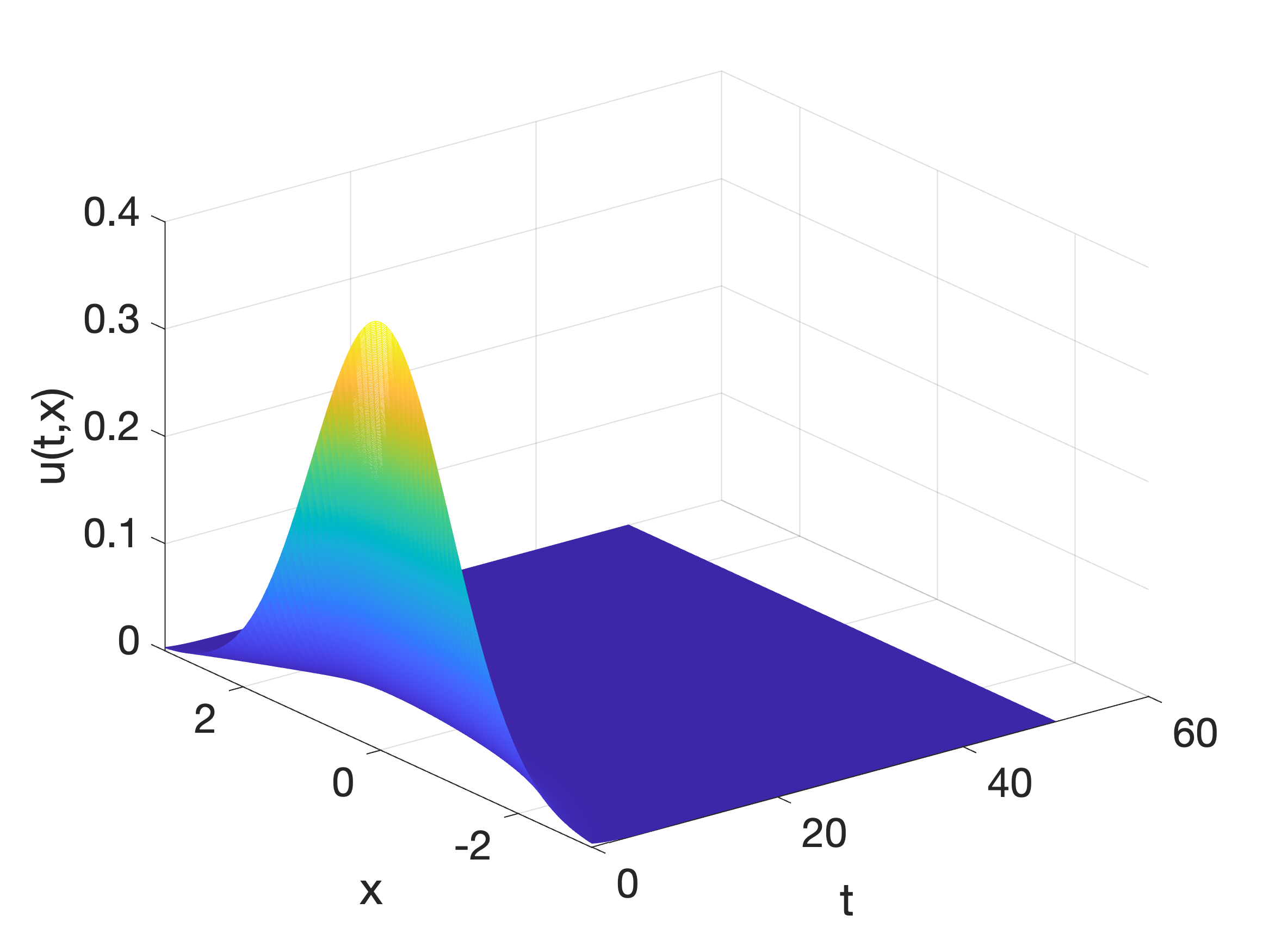
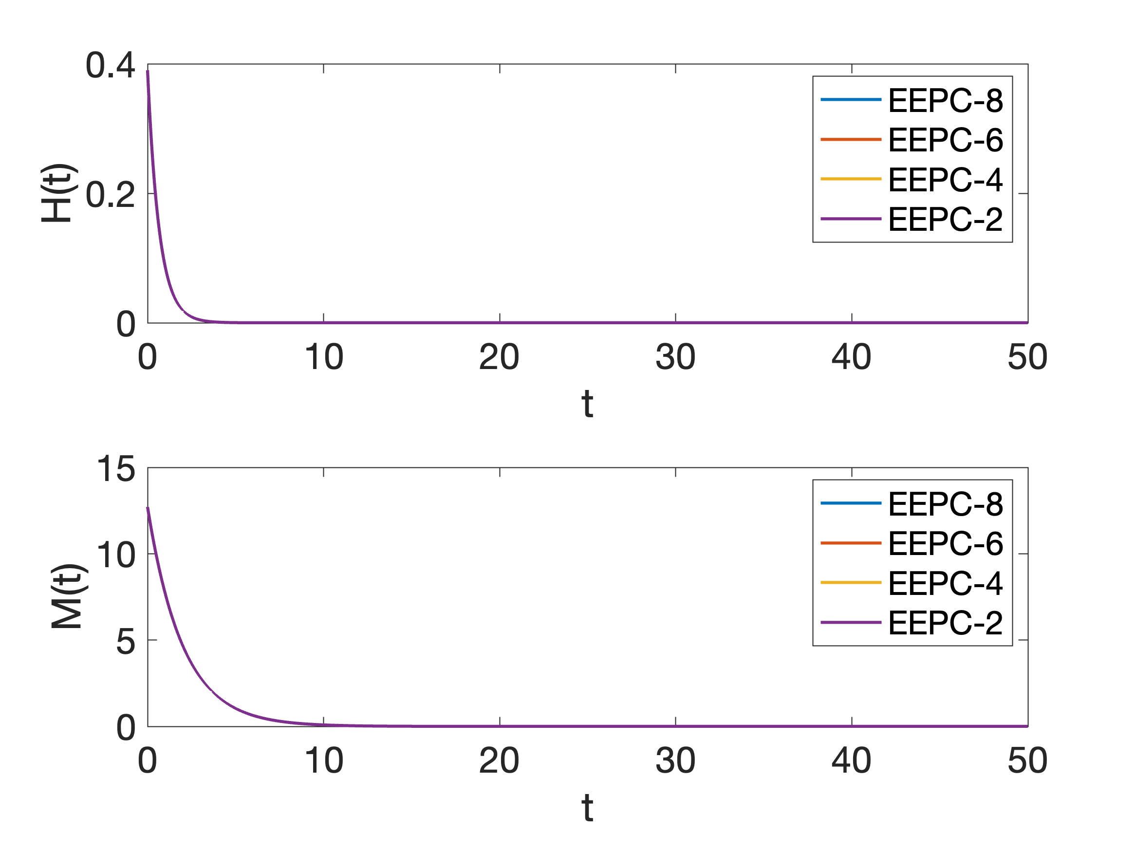
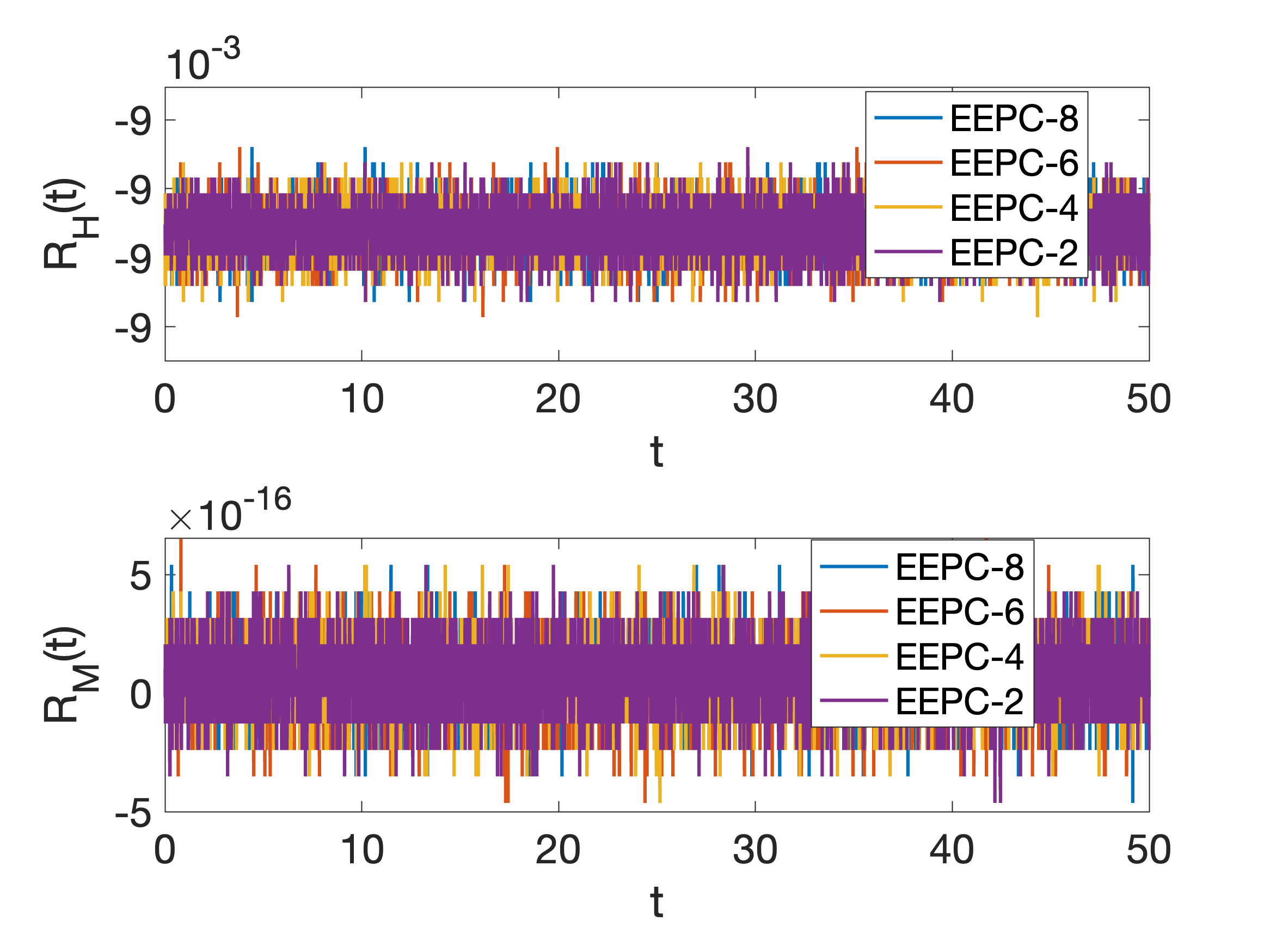
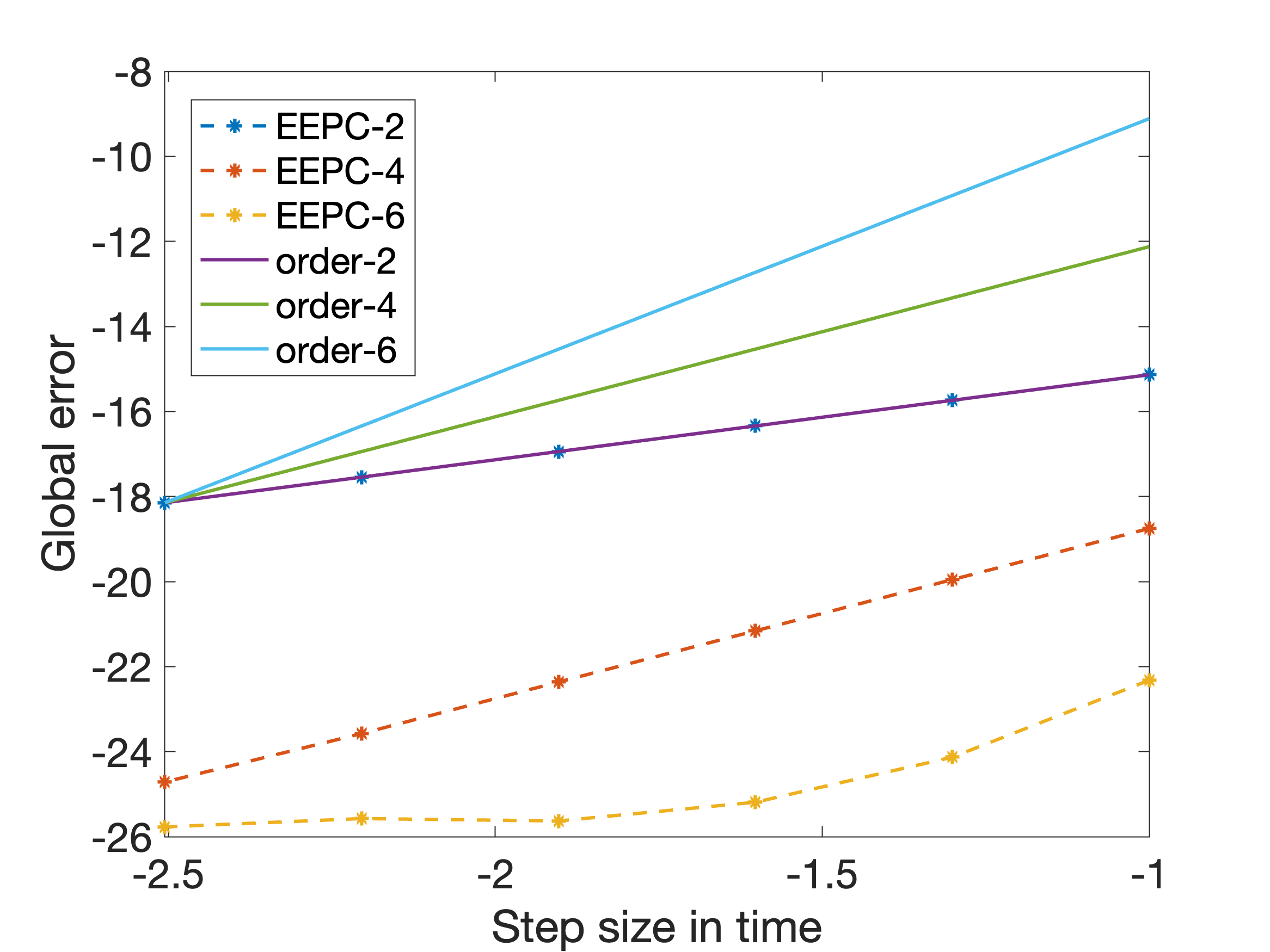
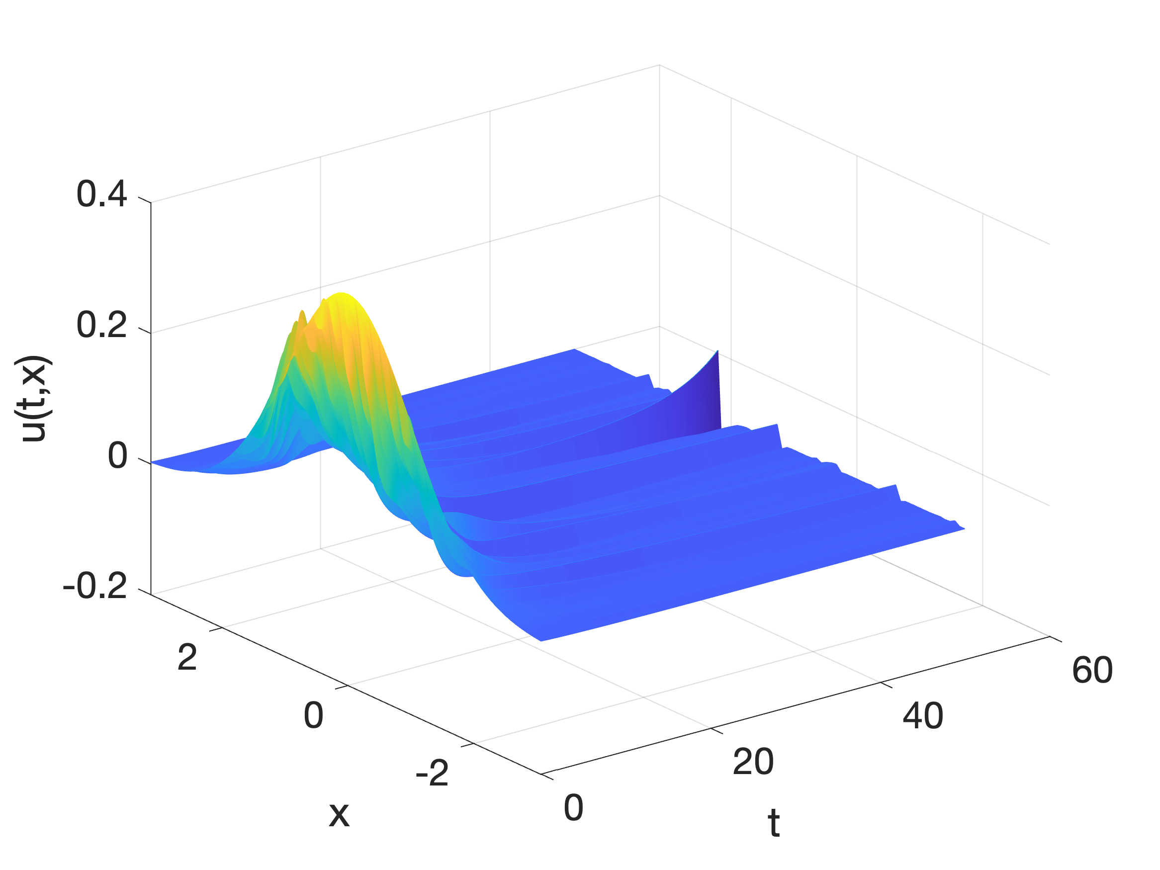
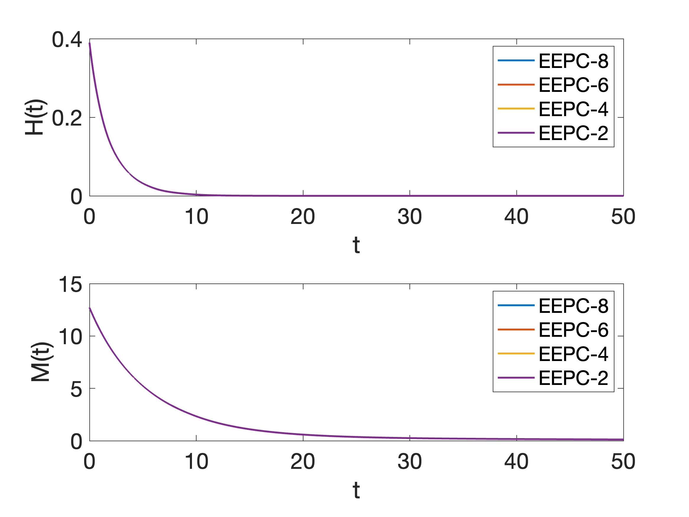
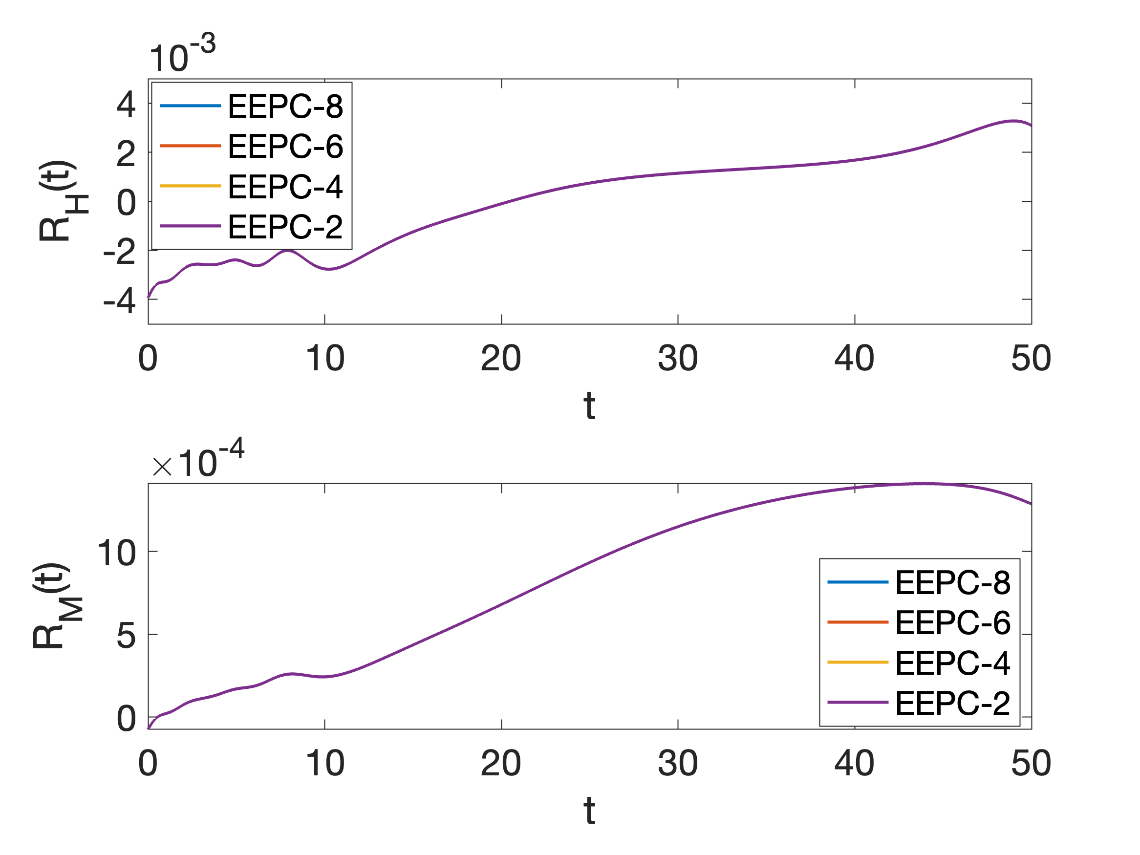
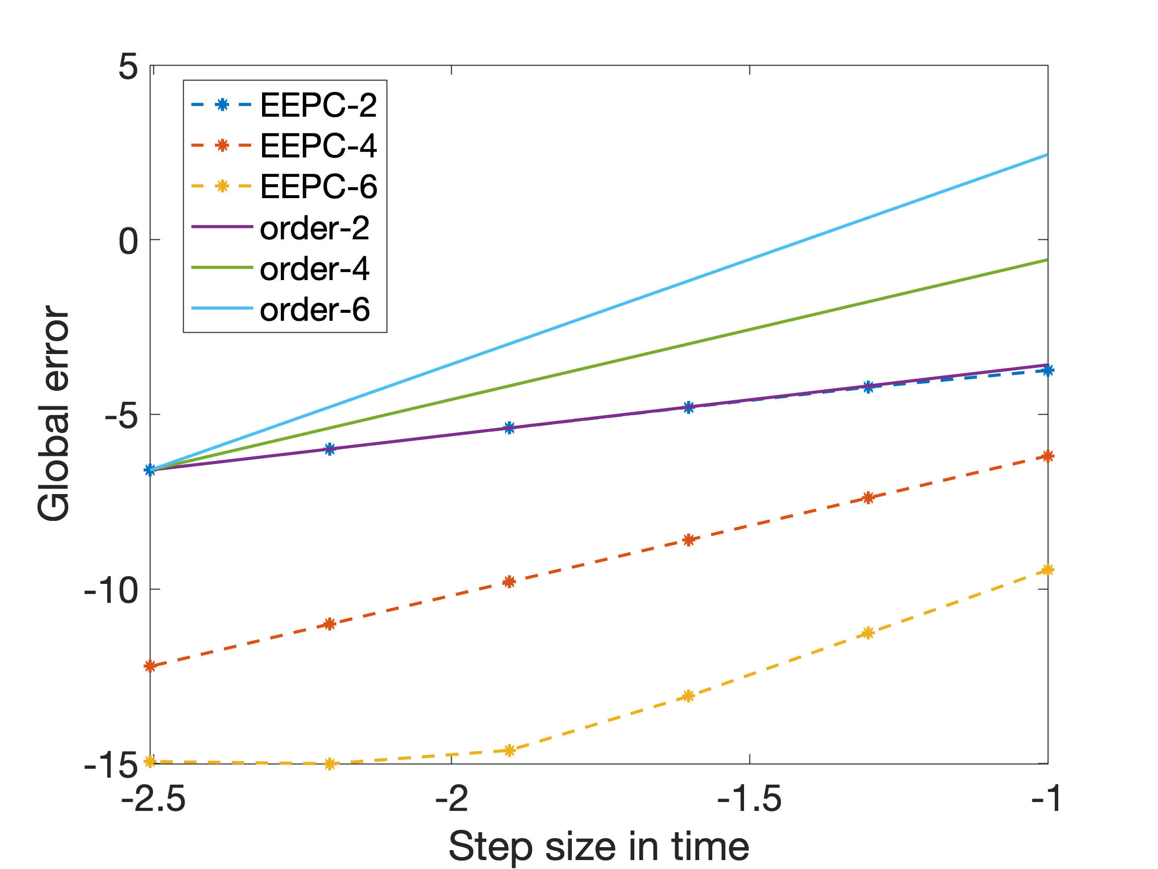
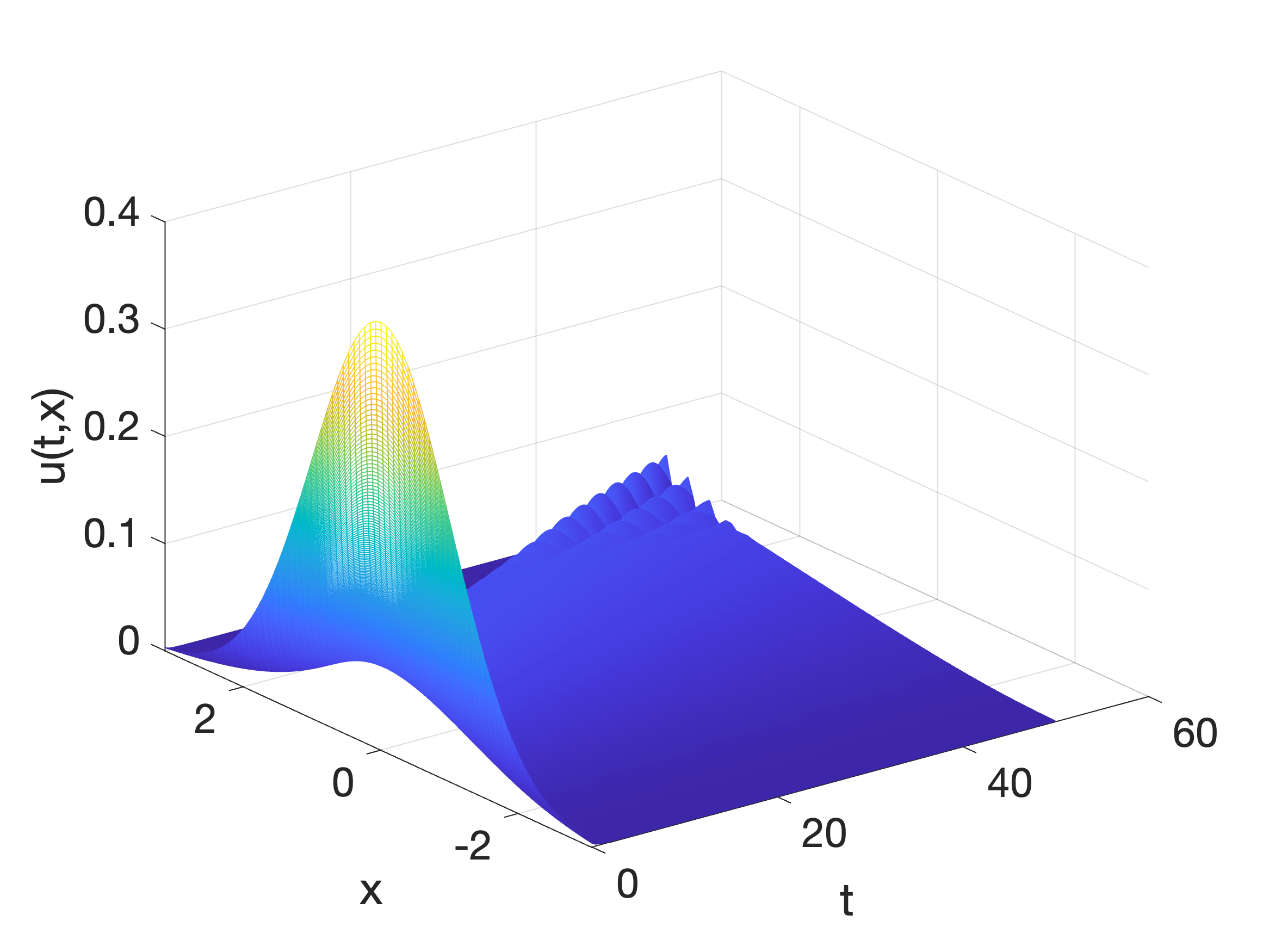
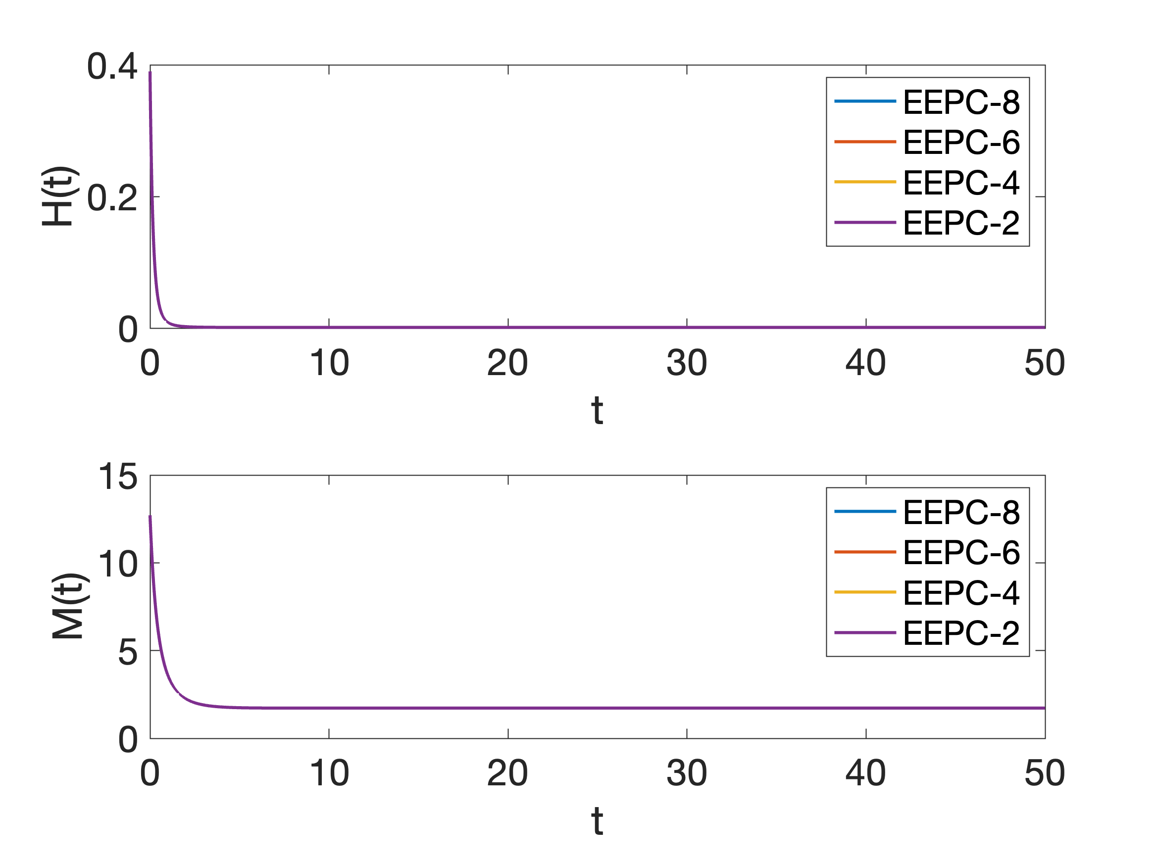
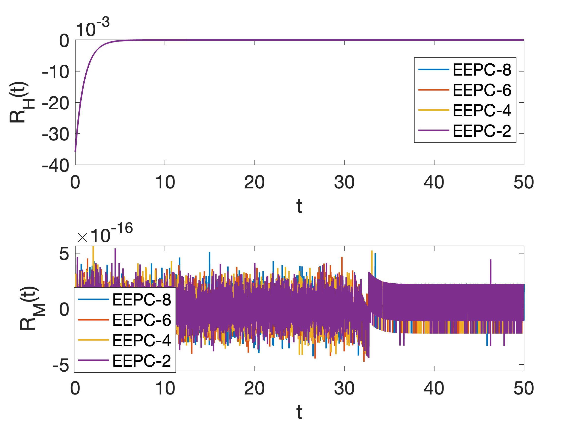
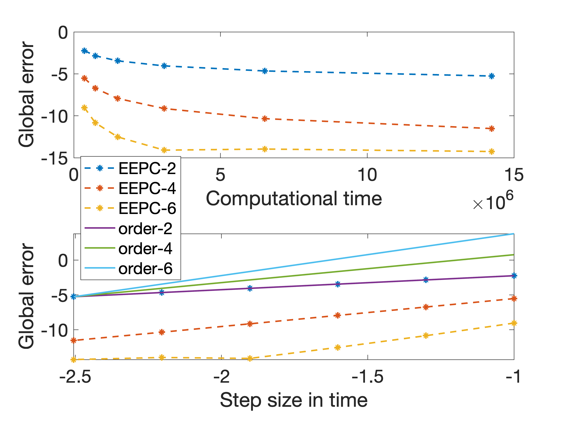
Case I: D(t) with constant equal diagonal elements . We observe that the proposed energy dissipation-preserving collocation methods of different orders produce similar numerical solutions. Figure 1(a) shows the numerical solution obtained by the second-order method. As illustrated, the amplitude of the numerical solution diminishes over time, indicating rapid damping. Figure 1(b) shows the exponential decay of both the Hamiltonian and mass over time. Figure 1(c) demonstrates that the proposed methods precisely preserve the dissipation rate of mass, while the dissipation rate of energy remains bounded and oscillatory throughout the integration. Figure 1(d) confirms the order of the proposed methods.
Case II: D(t) with constant unequal diagonal elements. In this scenario, we introduce a random perturbation to each default diagonal element of from Case I, within of the default values111Here, the random diagonal elements are ) using Matlab command.. Figure 2(a) presents the numerical solution obtained using the proposed method222Noting that the methods of different orders produce similar numerical solutions, we only present the numerical solution by the second order method here.. It is observed that the numerical solution exhibits reduced smoothness due to the unequal diagonal elements introduced by the random perturbations. The wave tends to damp over time, and negative values emerge during propagation. Figure 2(b) shows the decay of both energy and mass over time. Figure 2(c) demonstrates that when the condition in Theorem 1 is not satisfied, the mass decay rate can not be preserved. Figure 2(d) confirms the order of the proposed methods.
Case III: D(t) with time-dependent equal diagonal elements. We consider damped Burger’s equation 2(a) with damping factor . Figure 3(a) reports the numerical solution of the second-order exponential energy-preserving collocation method, and we observe similar numerical solutions by methods of different orders. As seen in Fig 3(b) and 3(a), both energy and mass decay over time exponentially and the amplitude of the numerical wave solutions diminishes. Figure 3(c) demonstrates that the proposed methods precisely preserve the dissipation rate of mass while the dissipation rate of energy remains bounded and oscillatory throughout the integration. Figure 3(d) confirms the order of the proposed methods.
4.2 Damped KdV equation
We consider the generalized KdV equation with Ekman damping, given by:
where are constant parameters [15]. This equation is often used in modeling of long-wavelength water waves and ion-acoustic waves. In the absence of the damping term (), the KdV equation exhibits a bi-Hamiltonian structure
with
and
Here, denotes the functional derivative of the Hamiltonian with respect to . We set , , and , and consider the spatial domain with and the integration interval with . The spatial and temporal domains are discretized using equal step sizes with and . The spatial grid points are and the vector is denoted as .
4.2.1 Semi-discrete system based on the first Hamiltonian form
When we consider a semi-discrete system based on the first Hamiltonian form, the condition in Theorem 1 is not satisfied. Consequently, the proposed methods do not exactly preserve the energy dissipation rate; however, the error should remain bounded and oscillatory for a diagonal matrix with small diagonal elements. The energy is discretized as:
and is approximated by . Thus, the semi-discrete system is given by:
| (14) |
with .
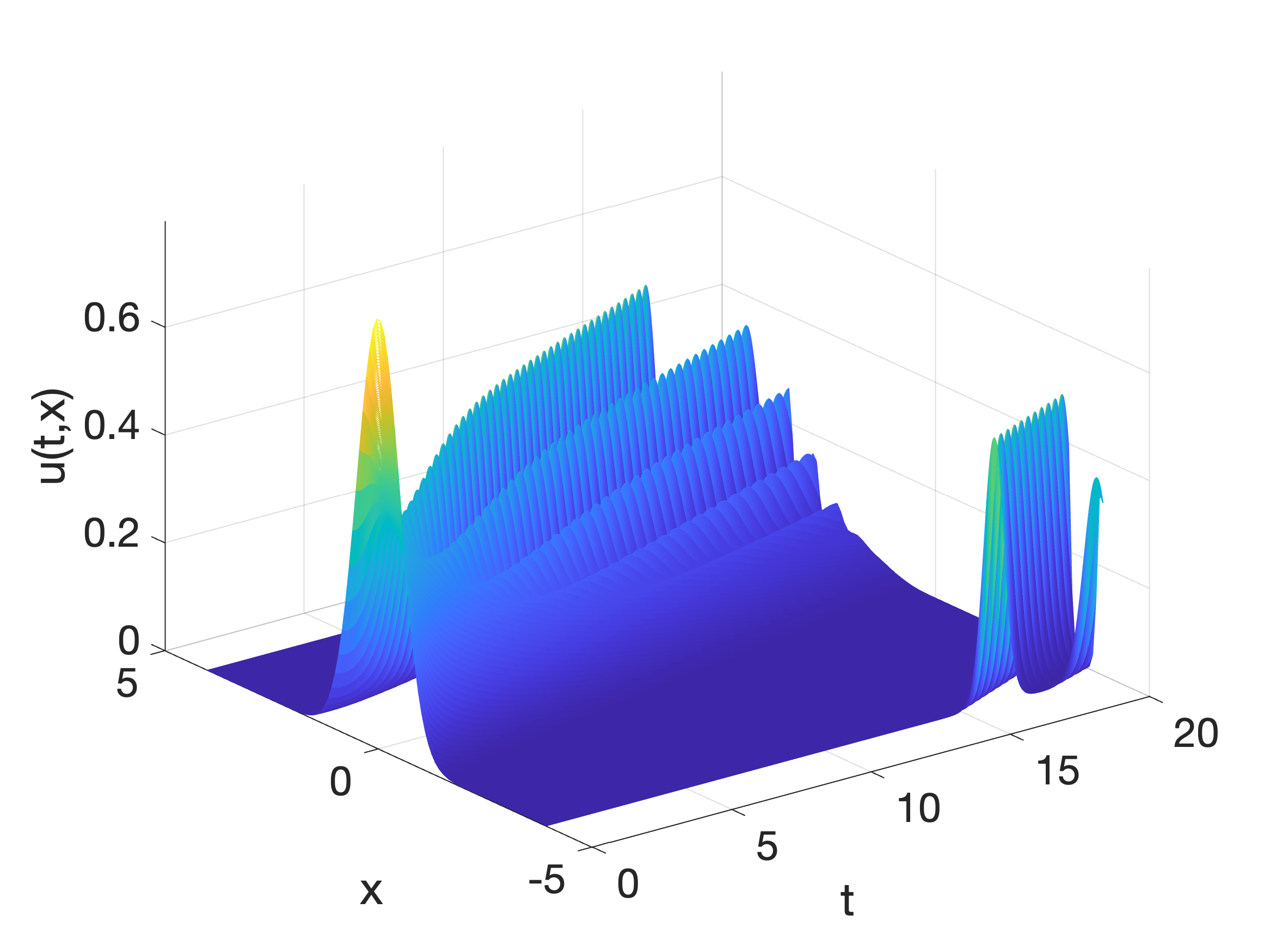
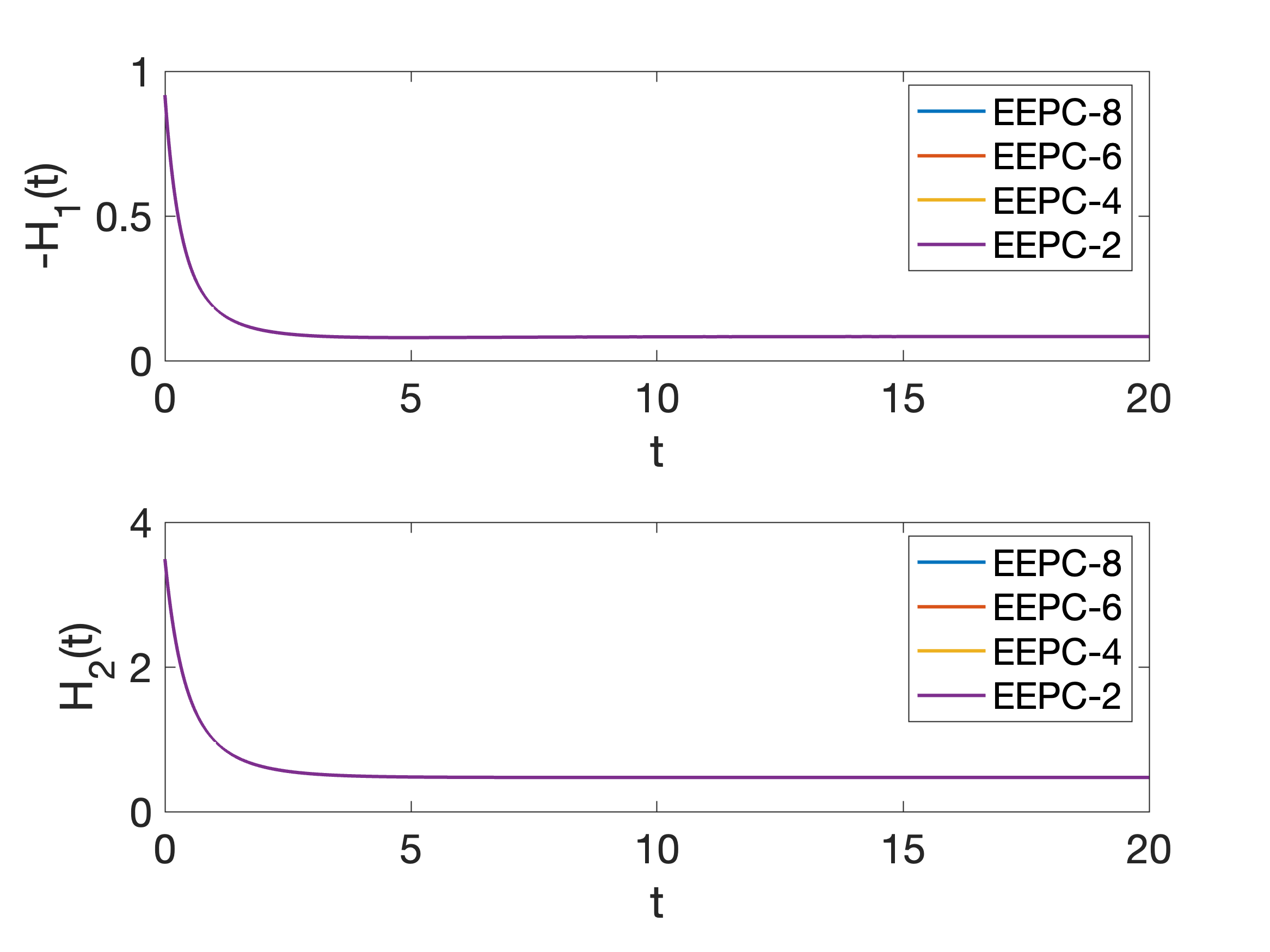
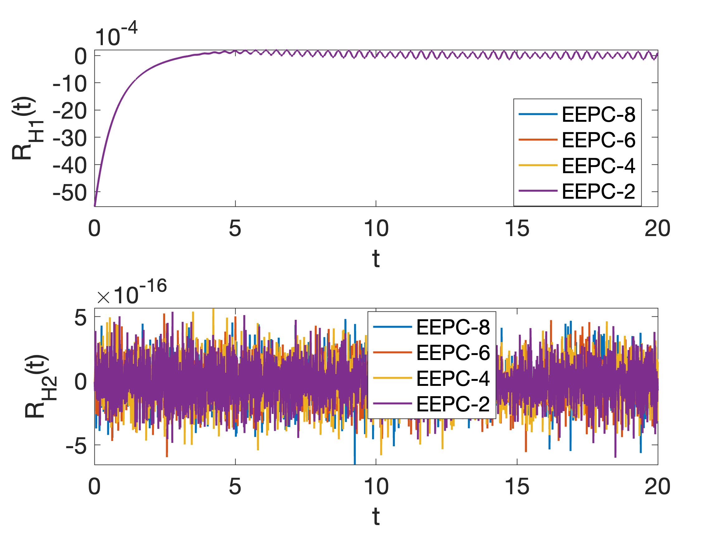
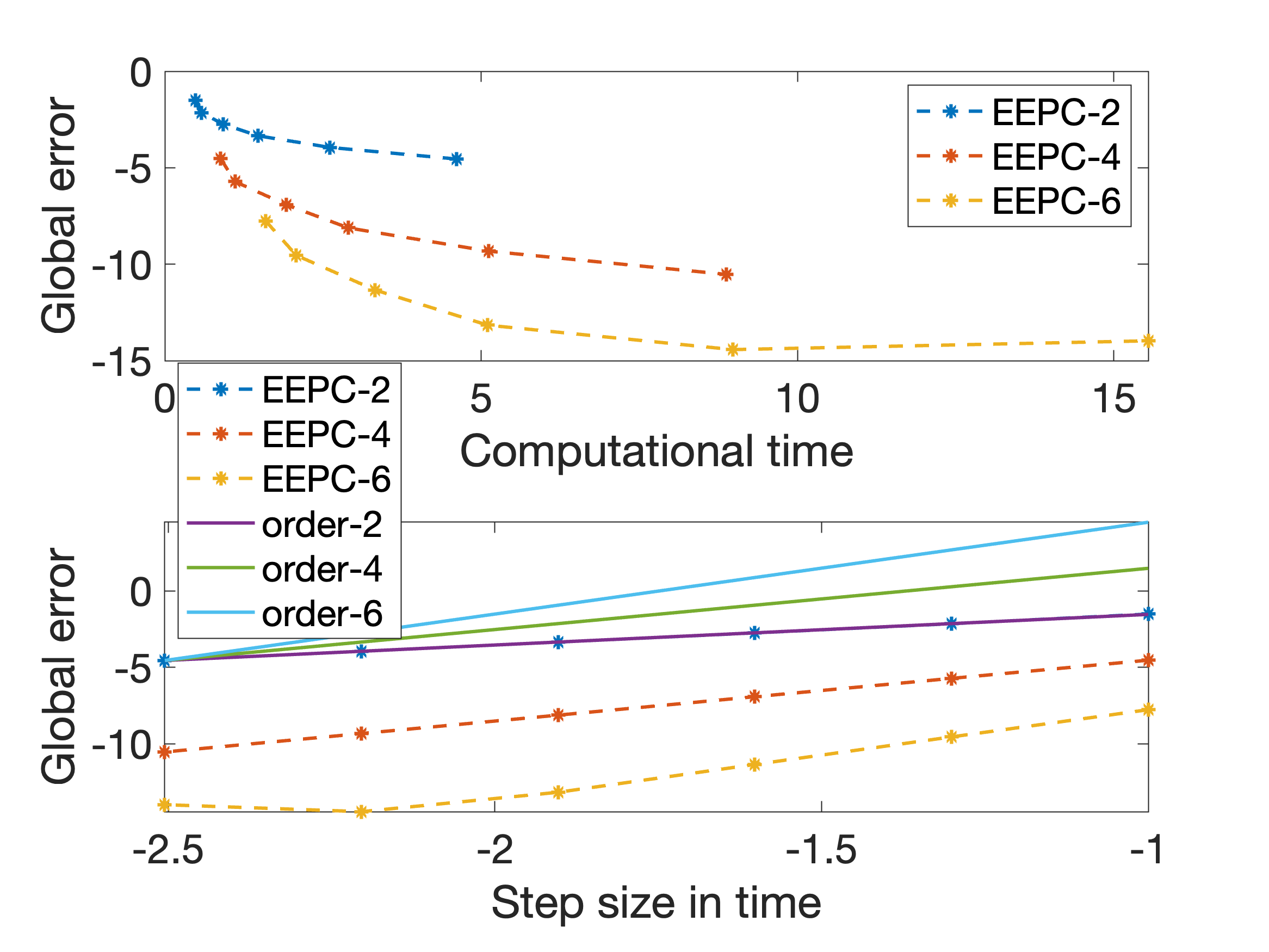
Figure 4 presents the numerical results for the damped KdV equation (14) using the proposed energy-preserving collocation methods of different orders. We observe that methods of different orders produce similar numerical solutions. Figure 4(a) shows the evolution of numerical wave over time by the second-order method. Figure 4(b) illustrates the exponential decay of both and ( is obtained by the discretization of Hamiltonian ) over time. Figure 4(c) demonstrates that the error of the numerical energy dissipation rate remains bounded and oscillatory throughout the integration. Figure 4(d) confirms the order of the proposed methods.
4.2.2 Semi-discrete system based on the second Hamiltonian form
We consider the semi-discrete Hamiltonian system based on the second Hamiltonian form. The term can be discretized as
and the term can be discretized as . Thus, the semi-discrete system is given by
| (15) |
which can be written as in the form of (1) with the skew-symmetric matrix as , the energy as and the coefficient matrix as .
is a conformal invariant for the damped Hamiltonian system (15) since satisfies
Therefore, the solution evolves on a sphere shrinking at an exponential rate. By Theorem 1, the proposed exponential methods can preserve the energy property, i.e., preserving the conformal invariant .
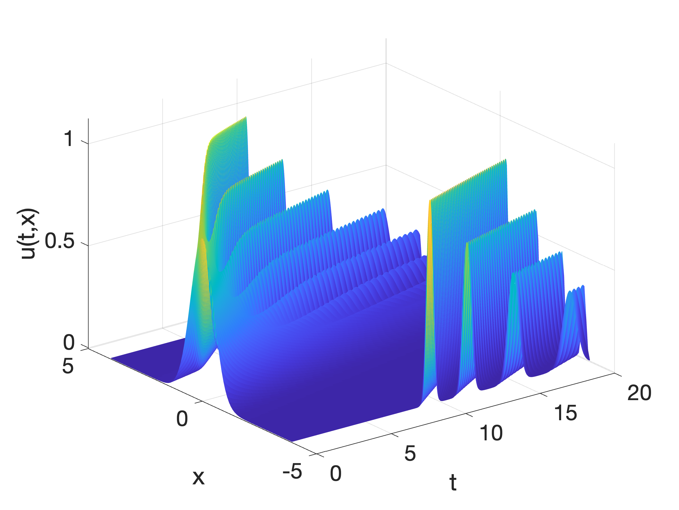
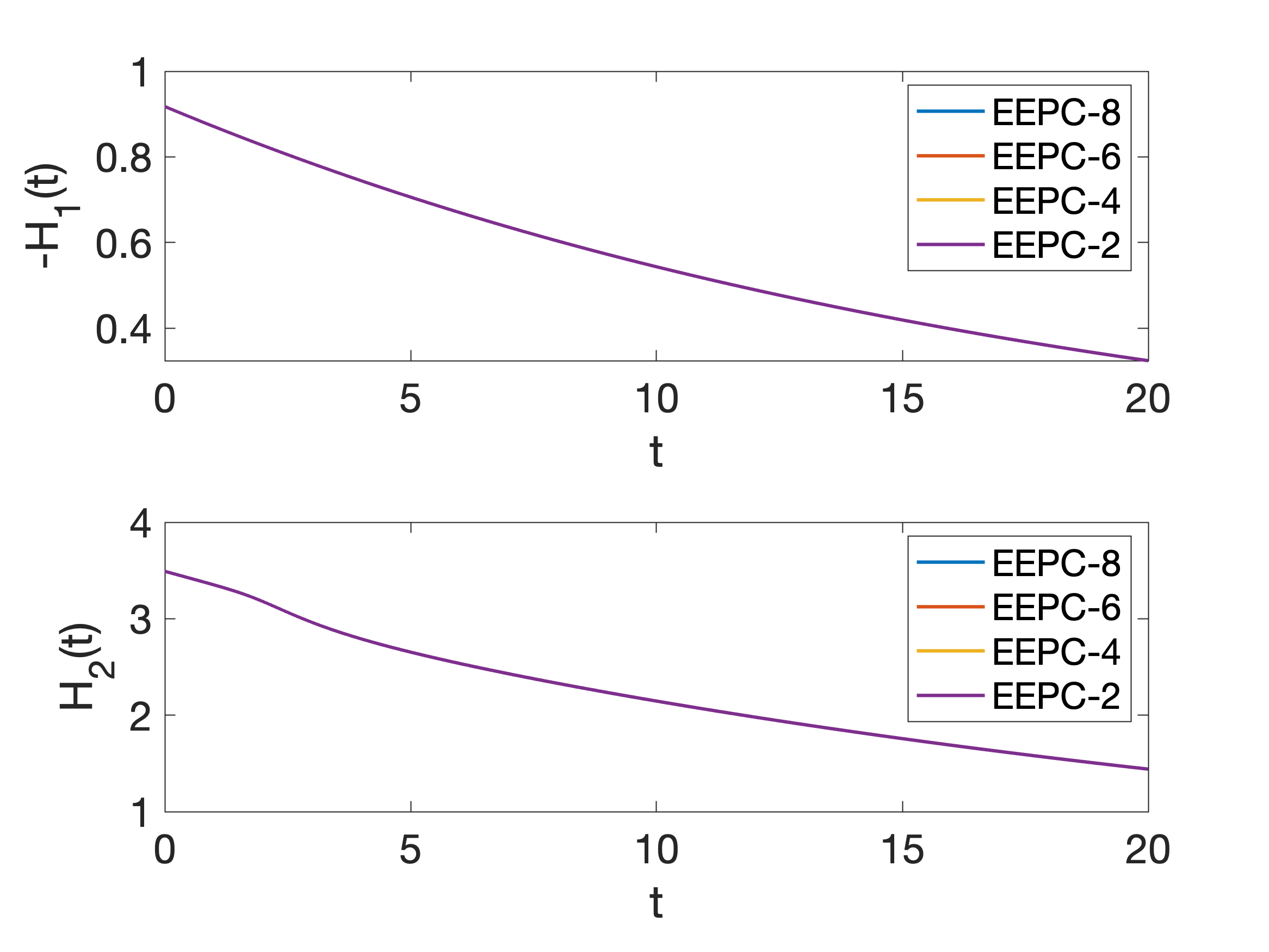
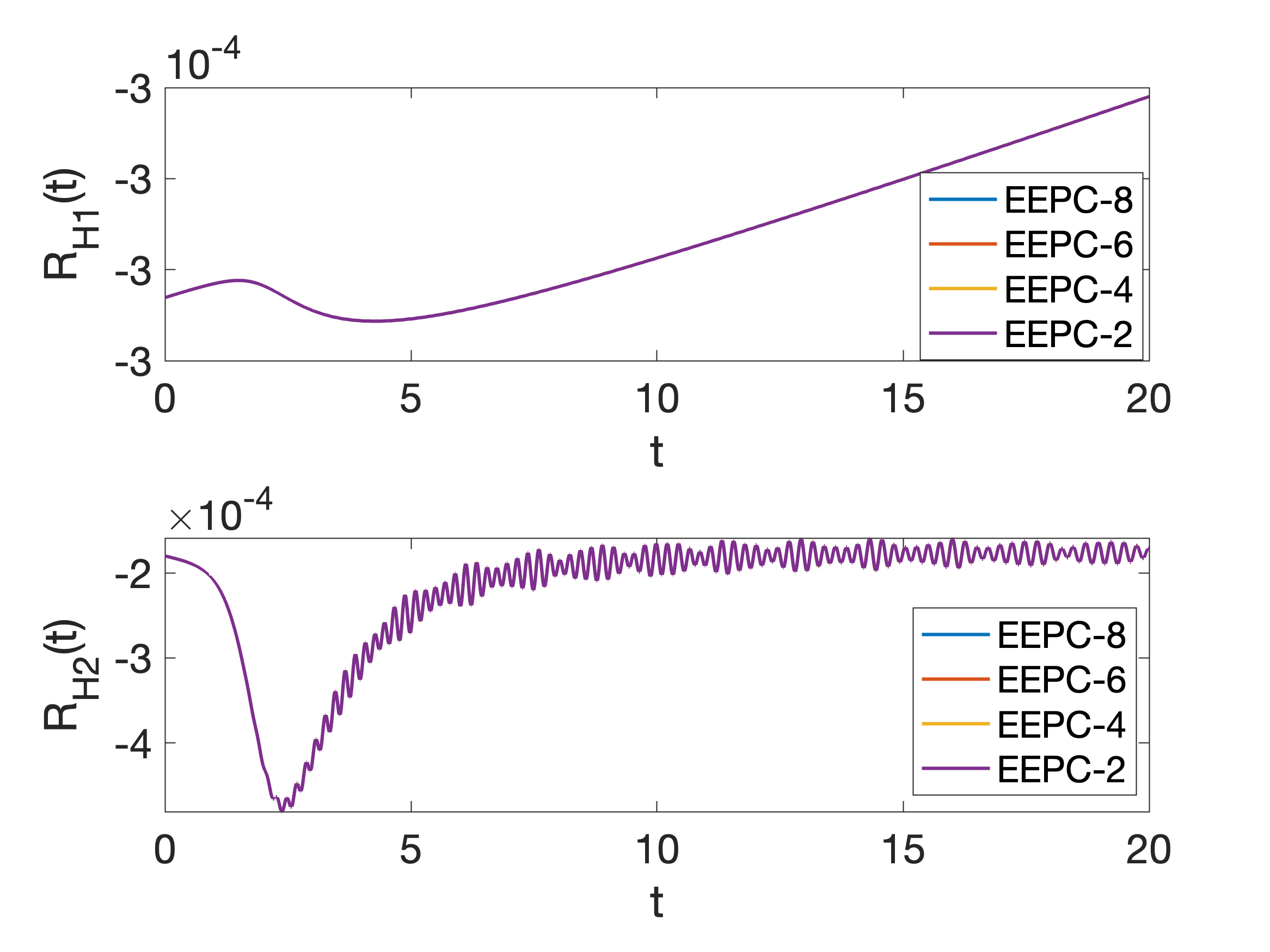
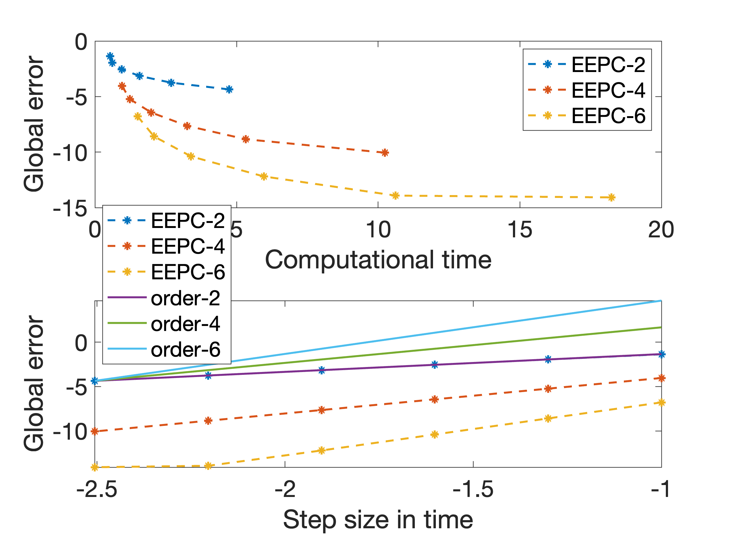
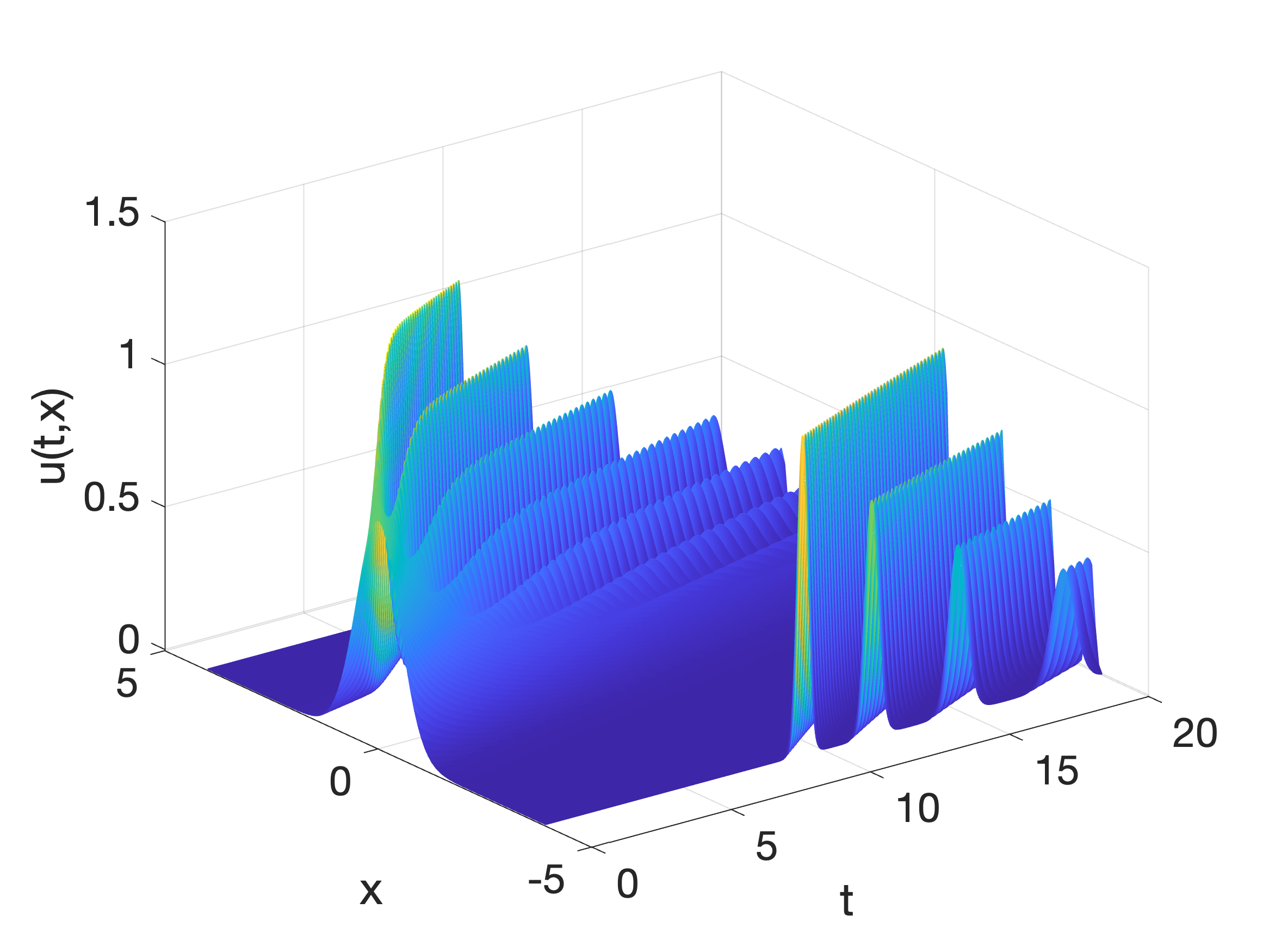
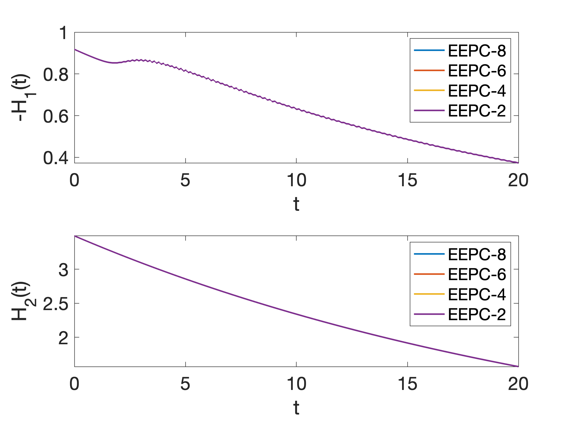
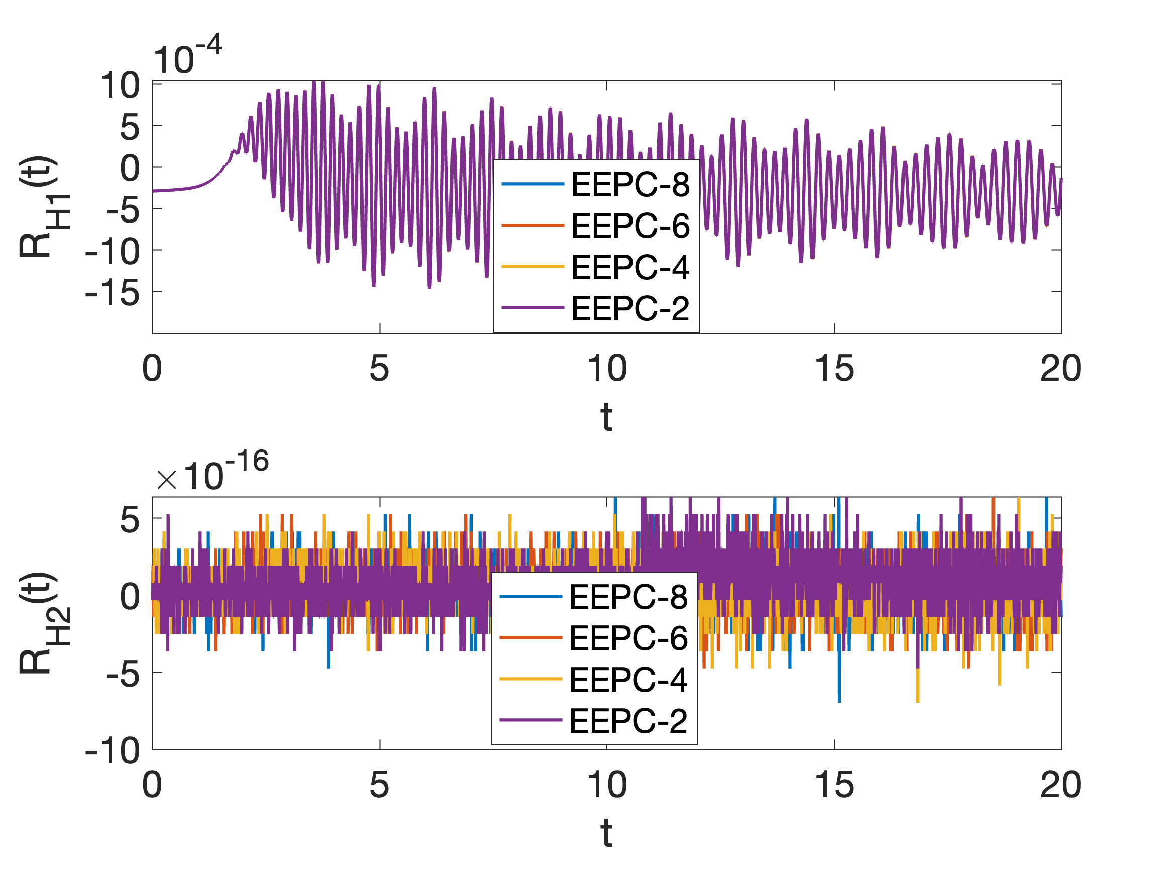
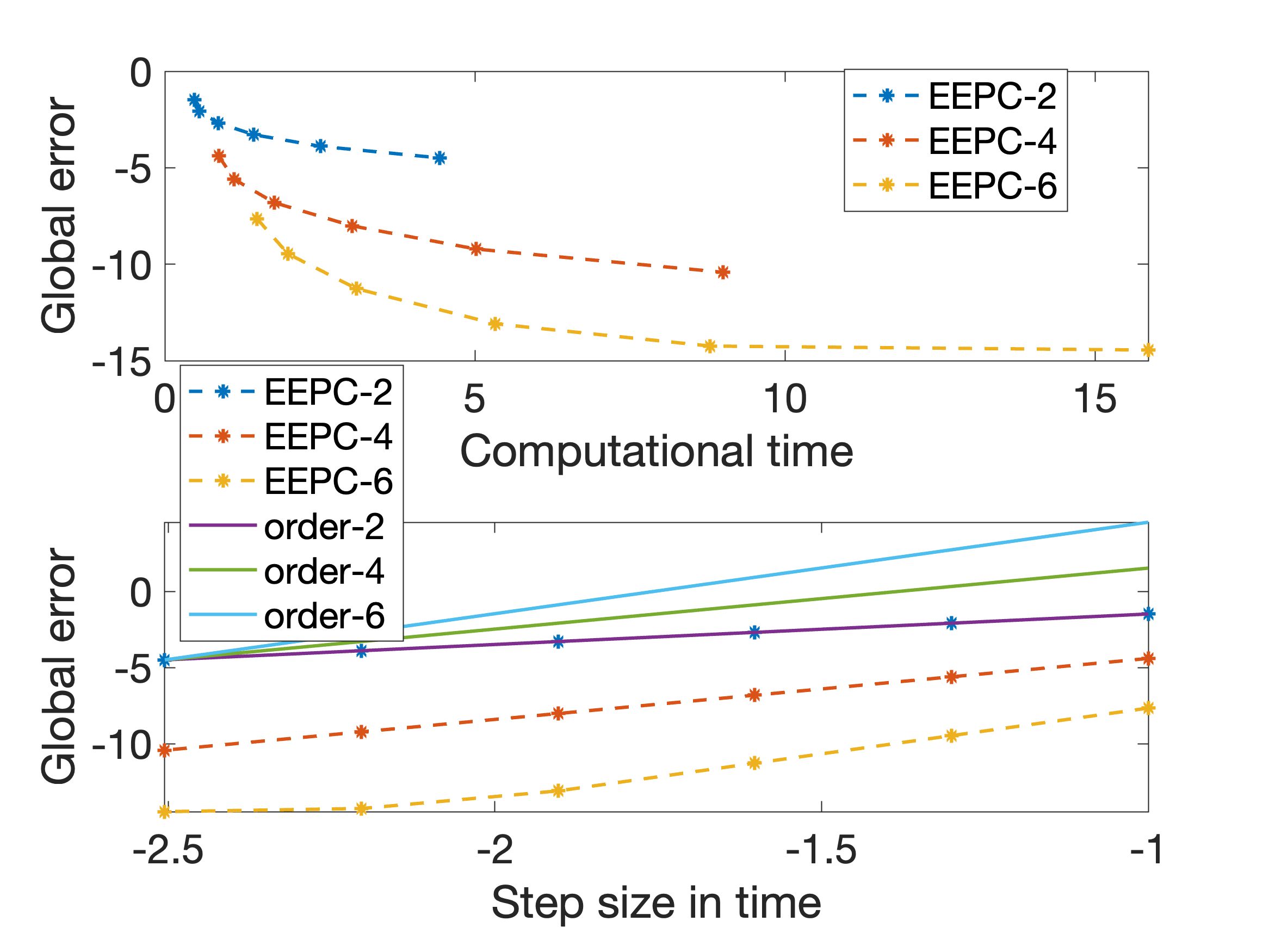
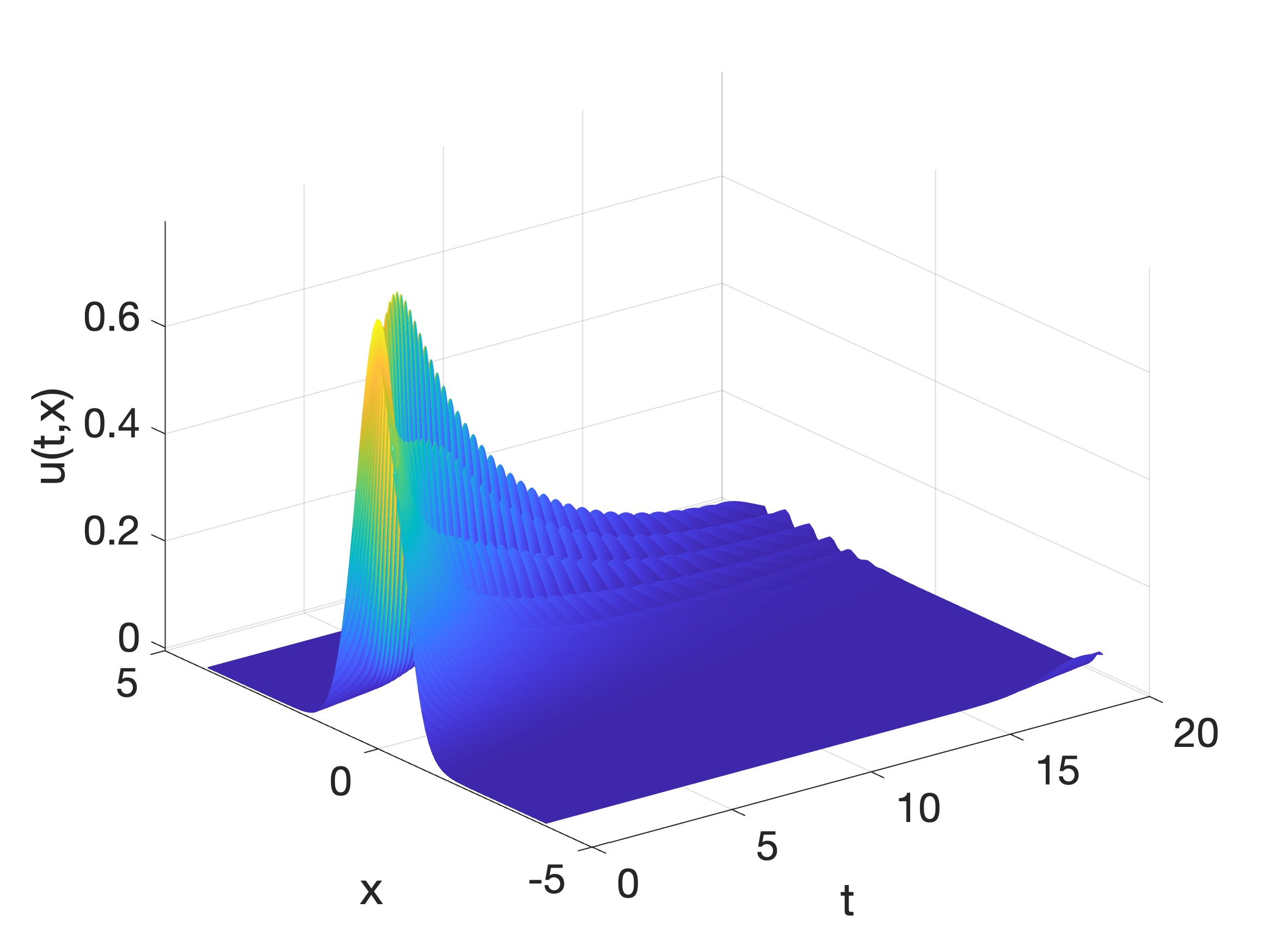
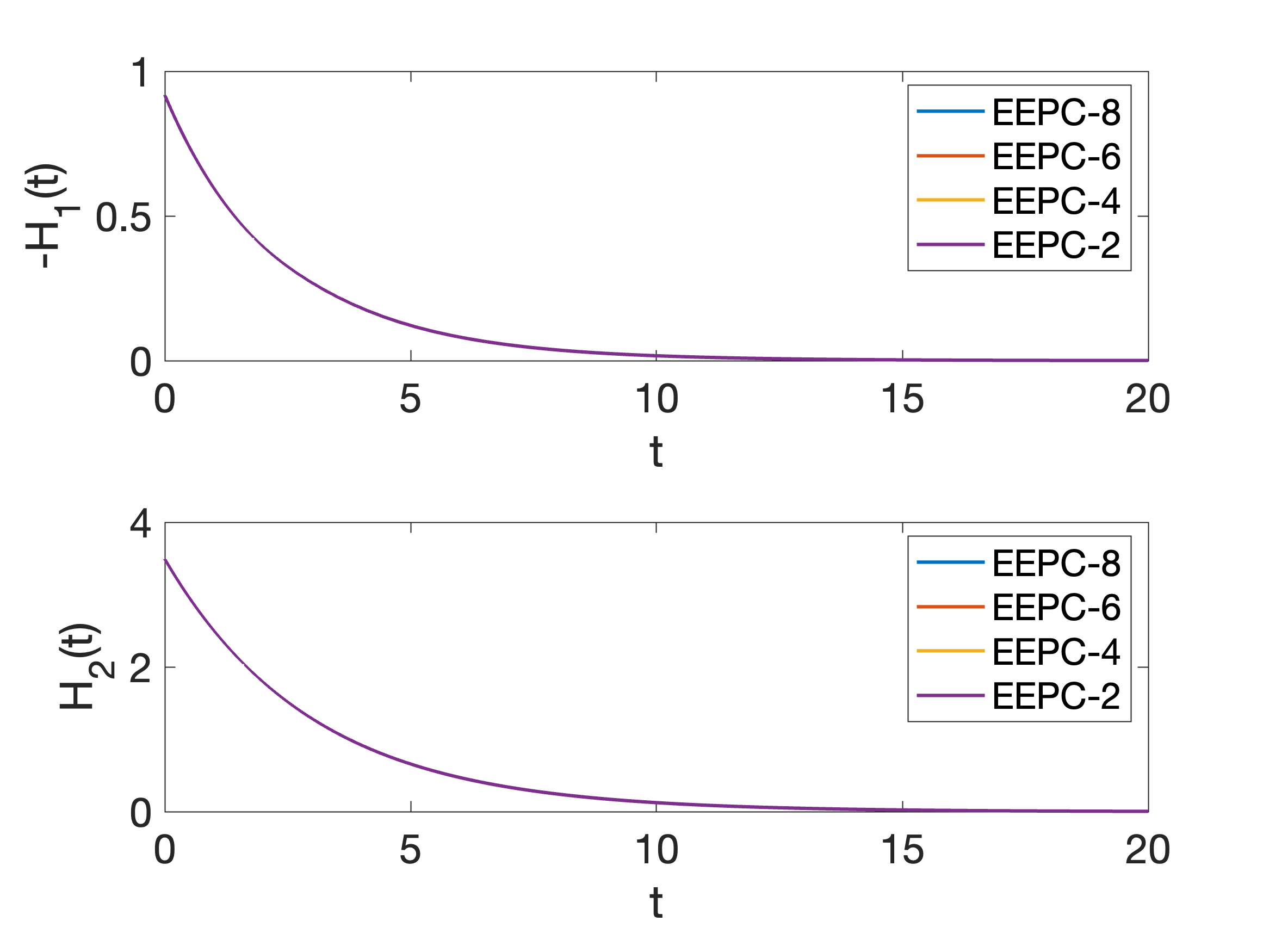
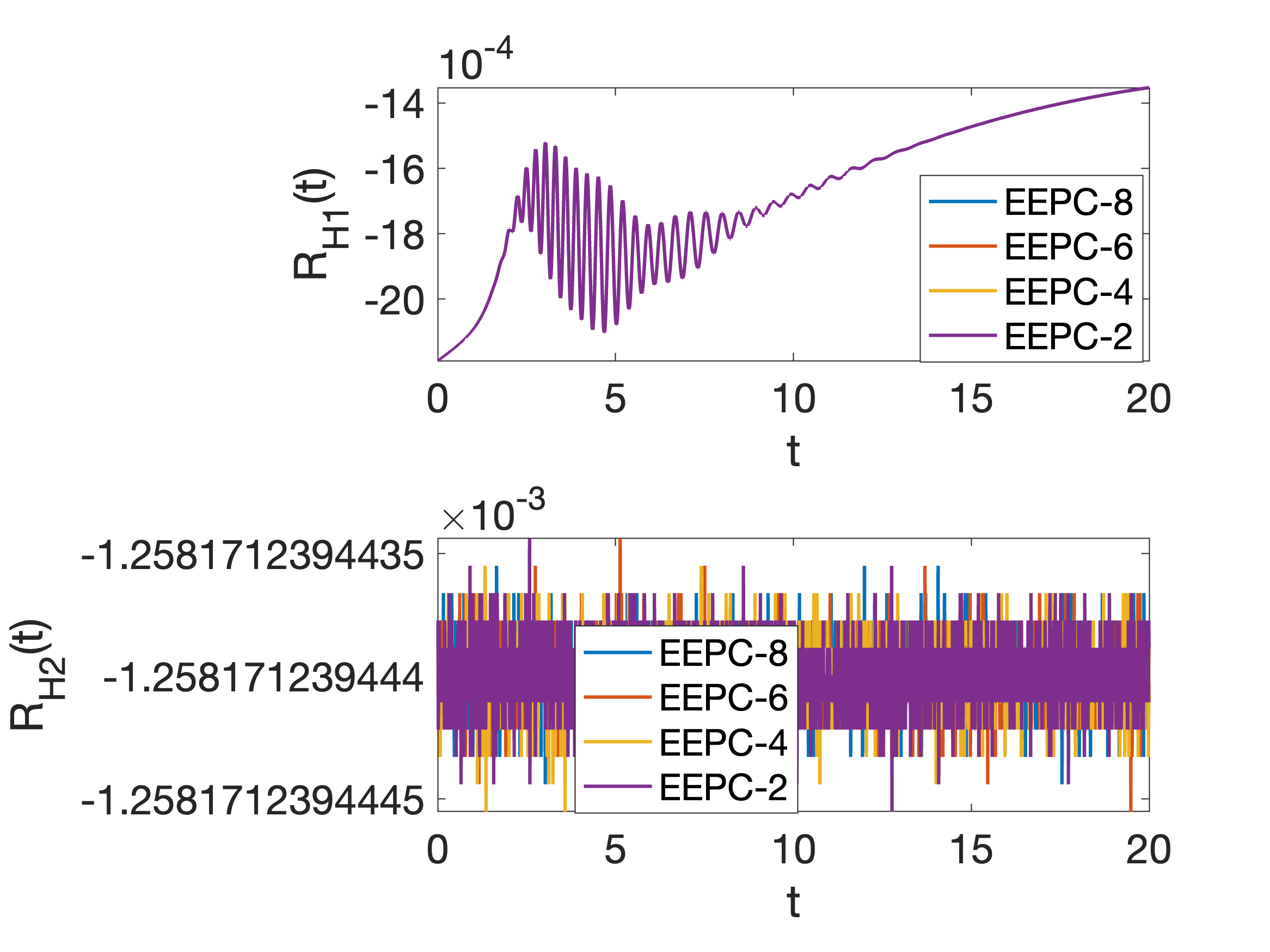
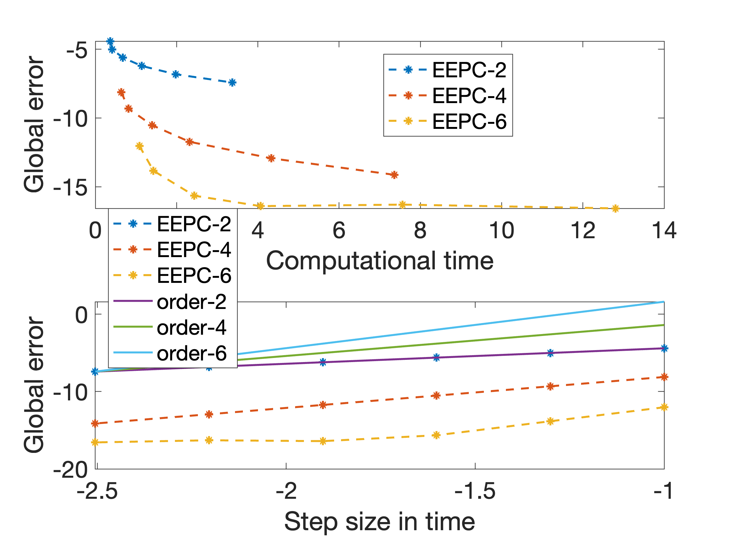
Case I: D(t) with constant equal diagonal elements . We apply the proposed methods to (15) following Remark 4. Fig 5(a) illustrates the numerical solution evolving over time. Figure 5(b) shows the dissipation of the energy function and over time. Here, we notice that the discrete energy does not strictly dissipate initially; however, it starts to dissipate stably after a few time steps. Figure 5(c) demonstrates that the dissipation rate of energy can be kept to machine accuracy while the error in the dissipation rate of remains bounded and oscillates. Figure 5(d) confirms the order of the proposed methods and also demonstrates the efficiency of the high-order method in achieving the same global error in less time.
With the second Hamiltonian form, the energy is quadratic, satisfying the conditions of Theorem 1 for all diagonal matrix with equal diagonal elements. However, this condition is not maintained for diagonal matrices with unequal diagonal elements, even in the simplest cases where are constant matrices. To numerically demonstrate these scenarios, we consider the second Hamiltonian form with two other sets of as follows.
Case II: D(t) with constant unequal diagonal elements . We introduce a random perturbation to each default diagonal element of in Case I within of the default value, resulting in unequal diagonal elements. As seen in Fig 6(a), there is a consistent damping of the numerical wave amplitude over time. Figure 6(b) depicts the decay of energy, which appears to be exponential. Figure 6(c) illustrates that the conservation property described in Theorem 1 is not maintained once the condition of the energy (or invariant in a more general sense) is not satisfied. However, we observe a constant difference between machine accuracy and the error computed from formula (12) based on the numerical dissipation rate of . This observation inspires further exploration of the correct underlying conservation law using more advanced technique such as deep learning [28]. Figure 6(d) confirms the order of the proposed methods and demonstrates that higher-order methods are more effective.
Case III: D(t) with time-dependent equal diagonal elements . We consider equal diagonal elements . Figure 7 shows the numerical solution, where we observe a decrease in wave amplitude followed by the spreading of the initial peak into smaller secondary peaks over time. In Figure 7(b), the energy decay appears exponential. Figure 7 demonstrates that the conservation property in Theorem 1 is maintained for diagonal matrices as long as their diagonal elements are equal, regardless of whether they are constant. Figure 7(d) confirms the order of the proposed methods, also showing that higher-order methods are more effective.
5 Conclusion
In this study, arbitrarily high-order structure-preserving methods have been developed for damped Hamiltonian systems by combining exponential integrators with energy-preserving collocation methods. These integrators maintain the energy dissipation ratio introduced by damping terms, exhibiting notable advantages in terms of efficiency, accuracy, and stability. This makes them well-suited for solving complex and large-scale problems. The presented results are based on damped Hamiltonian systems with a diagonal coefficient matrix of special forms. For certain cases, such as the KdV equation with having constant unequal diagonal elements, numerical simulations suggest the existence of particular energy dissipation laws, despite the challenge in uncovering such energy conservation laws for the true solution. This observation prompts further investigation into the underlying physical laws using more advanced techniques. Additionally, extending suitable structure-preserving methods for more general Hamiltonian systems with varying damping terms remains an open research question for the future.
References
- [1] H.-S. Chang, U. Halder, E. Gribkova, A. Tekinalp, N. Naughton, M. Gazzola, P. G. Mehta, Controlling a cyberoctopus soft arm with muscle-like actuation, in: 2021 60th IEEE Conference on Decision and Control (CDC), IEEE, 2021, pp. 1383–1390.
- [2] R. Temam, Infinite-dimensional dynamical systems in mechanics and physics, Vol. 68, Springer Science & Business Media, 2012.
- [3] E. Hairer, M. Hochbruck, A. Iserles, C. Lubich, Geometric numerical integration, Oberwolfach Reports 3 (1) (2006) 805–882.
- [4] B. Leimkuhler, S. Reich, Simulating Hamiltonian dynamics, Vol. 14, Cambridge university press, 2004.
- [5] R. McLachlan, M. Perlmutter, Conformal Hamiltonian systems, Journal of Geometry and Physics 39 (4) (2001) 276–300.
- [6] R. I. McLachlan, G. R. W. Quispel, Splitting methods, Acta Numerica 11 (2002) 341–434.
- [7] K. Modin, G. Söderlind, Geometric integration of Hamiltonian systems perturbed by rayleigh damping, BIT Numerical Mathematics 51 (2011) 977–1007.
- [8] A. Bhatt, D. Floyd, B. E. Moore, Second order conformal symplectic schemes for damped Hamiltonian systems, Journal of Scientific Computing 66 (2016) 1234–1259.
- [9] Y. Sun, Z. Shang, Structure-preserving algorithms for birkhoffian systems, Physics Letters A 336 (4-5) (2005) 358–369.
- [10] A. Bhatt, B. E. Moore, Structure-preserving exponential Runge–Kutta methods, SIAM Journal on Scientific Computing 39 (2) (2017) A593–A612.
- [11] B. E. Moore, Conformal multi-symplectic integration methods for forced-damped semi-linear wave equations, Mathematics and Computers in Simulation 80 (1) (2009) 20–28.
- [12] B. E. Moore, L. Noreña, C. M. Schober, Conformal conservation laws and geometric integration for damped Hamiltonian PDEs, Journal of Computational Physics 232 (1) (2013) 214–233.
- [13] A. Bhatt, B. E. Moore, Exponential integrators preserving local conservation laws of PDEs with time-dependent damping/driving forces, Journal of Computational and Applied Mathematics 352 (2019) 341–351.
- [14] W. Cai, H. Zhang, Y. Wang, Modelling damped acoustic waves by a dissipation-preserving conformal symplectic method, Proceedings of the Royal Society A: Mathematical, Physical and Engineering Sciences 473 (2199) (2017) 20160798.
- [15] A. Bhatt, Projected exponential runge–kutta methods for preserving dissipative properties of perturbed constrained hamiltonian systems, Journal of Computational and Applied Mathematics 394 (2021) 113556.
- [16] B. E. Moore, Exponential integrators based on discrete gradients for linearly damped/driven poisson systems, Journal of Scientific Computing 87 (2021) 1–18.
- [17] M. Uzunca, B. Karasözen, Linearly implicit exponential integrators for damped Hamiltonian PDEs, arXiv preprint arXiv:2309.14184 (2023).
- [18] E. Celledoni, V. Grimm, R. I. McLachlan, D. I. McLaren, D. O’Neale, B. Owren, G. Quispel, Preserving energy resp. dissipation in numerical PDEs using the “average vector field” method, Journal of Computational Physics 231 (20) (2012) 6770–6789.
- [19] E. Hairer, C. Lubich, Energy-diminishing integration of gradient systems, IMA Journal of Numerical Analysis 34 (2) (2014) 452–461.
- [20] Y.-W. Li, X. Wu, Exponential integrators preserving first integrals or Lyapunov functions for conservative or dissipative systems, SIAM Journal on Scientific Computing 38 (3) (2016) A1876–A1895.
- [21] B. Wang, X. Wu, Exponential collocation methods for conservative or dissipative systems, Journal of Computational and Applied Mathematics 360 (2019) 99–116.
- [22] L. Li, A new symmetric linearly implicit exponential integrator preserving polynomial invariants or Lyapunov functions for conservative or dissipative systems, Journal of Computational Physics 449 (2022) 110800.
- [23] E. Celledoni, R. I. McLachlan, B. Owren, G. R. W. Quispel, Geometric properties of Kahan’s method, Journal of Physics A: Mathematical and Theoretical 46 (2) (2012) 025201.
- [24] S. Eidnes, L. Li, S. Sato, Linearly implicit structure-preserving schemes for Hamiltonian systems, Journal of Computational and Applied Mathematics 387 (2021) 112489.
- [25] M. Dahlby, B. Owren, A general framework for deriving integral preserving numerical methods for PDEs, SIAM Journal on Scientific Computing 33 (5) (2011) 2318–2340.
- [26] R. I. McLachlan, B. N. Ryland, Y. Sun, High order multisymplectic Runge–Kutta methods, SIAM Journal on Scientific Computing 36 (5) (2014) A2199–A2226.
- [27] E. Hairer, Energy-preserving variant of collocation methods, JNAIAM 5 (1-2) (2010) 73–84.
- [28] S. Eidnes, A. J. Stasik, C. Sterud, E. Bøhn, S. Riemer-Sørensen, Pseudo-hamiltonian neural networks with state-dependent external forces, Physica D: Nonlinear Phenomena 446 (2023) 133673.