An extra gradient Anderson-accelerated algorithm for pseudomonotone variational inequalities
Abstract.
This paper proposes an extra gradient Anderson-accelerated algorithm for solving pseudomonotone variational inequalities, which uses the extra gradient scheme with line search to guarantee the global convergence and Anderson acceleration to have fast convergent rate. We prove that the sequence generated by the proposed algorithm from any initial point converges to a solution of the pseudomonotone variational inequality problem without assuming the Lipschitz continuity and contractive condition, which are used for convergence analysis of the extra gradient method and Anderson-accelerated method, respectively in existing literatures. Numerical experiments, particular emphasis on Harker-Pang problem, fractional programming, nonlinear complementarity problem and PDE problem with free boundary, are conducted to validate the effectiveness and good performance of the proposed algorithm comparing with the extra gradient method and Anderson-accelerated method.
Key words and phrases:
Pseudomonotone variational inequality, extra gradient algorithm, Anderson acceleration, sequence convergence, PDE problem with free boundary2020 Mathematics Subject Classification:
Primary 47J20, 65K10, 65Y20; Secondary 90C30, 65H101. Introduction
In this paper, we consider the following variational inequality (VI) problem: find an such that
| (1.1) |
where is a closed convex set of and is a continuous function, and pseudomonotone on , but not necessarily smooth or even Lipschitz continuous. Throughout this paper, we denote problem (1.1) by and the solution set of (1.1) by , and assume
Variational inequalities (VIs) provide a unified framework for representing various important concepts in applied mathematics such as nonlinear equation systems, complementarity problems, optimality conditions for optimization problems and network equilibrium problems. Thus, VIs have a wide range of applications in physics, economics, engineering sciences and so on [6, 14, 21, 33, 39]. One of the most interesting topics in VIs is to develop efficient and fast iterative algorithms to find solutions.
As a class of effective numerical methods for solving VIs, projection methods have received a lot of attention from many researchers. The earliest projection method for solving is the gradient projection (PG) method [18]
| (1.2) |
where denotes the projection onto the set and . To guarantee the convergence of PG method, is often assumed to be either cocoercive or strongly monotone, in addition to being -Lipschitz continuous on 111 is called -Lipschitz continuous on if for any .. An example given in [16] showed that the sequence generated by PG method may be divergent if is only monotone and -Lipschitz continuous. In order to weaken the strong monotonicity of , many projection methods have been proposed to solve monotone VIs [10, 11, 30, 31, 41, 42, 43]. Very recently, developing algorithms for different nonmonotone VIs has attracted great attention due to applications in machine learning [9, 28, 36, 37, 40, 45]. In this paper, we focus on solving with a pseudomonotone , which is a widely used class of nonmonotone VIs. A most commonly used algorithm in the literatures for solving pseudomonotone VIs is the Korpelevich’s extra gradient (EG) method [27]. EG method was originally used to solve with a monotone and -Lipschitz continuous , and was later extended by Pang and Facchinei [16] to solve the pseudomonotone VIs. After that, EG method has been intensively studied and extended in various ways [9, 10, 11, 15, 19, 23, 28, 29, 31, 36, 37, 40, 43, 44]. It is worth pointing out that besides the -Lipschitz continuity of on , some other conditions on are often required to guarantee the convergence of EG method and its variants, such as Minty condition, quasimonotonicity, pseudomonotonicity and weak monotonicity.
To the best of our knowledge, current research on the Minty condition cannot simultaneously provide an analysis of both sequence convergence and convergence rates. One of the main objectives of this paper is to design an algorithm that ensures both the sequence convergence and a fast convergence rate under the pseudomonotonicity on of . In subsection 1.1, we will review and summarize the development of EG methods for nonmonotone VIs in recent years in detail. A summary of some main comparisons is provided in Table 1.
It is known that is equivalent to the following fixed point problem [16]:
| (1.3) |
where . Thus, the study of PG method in (1.2), which is a fixed point method, can help to improve the performance of the algorithms for solving VIs. Anderson acceleration is efficient to improve the convergence rate of fixed point methods, but the existing convergence analysis of Anderson acceleration requires the fixed point mapping to be contractive and piecewise smooth. However, due to the nonmonotonicity of , the mapping is not contractive, and may be even expansive, which means that we cannot directly use Anderson acceleration to solve the corresponding fixed point problem of in (1.3). Moreover, is nonsmooth, because of the projection operator . In this paper, we introduce Anderson acceleration technique into EG method to ensure the global sequence convergence of the algorithm and improve the convergence rate of EG method. We will review the recent development of Anderson acceleration for fixed point problems in subsection 1.2.
1.1. EG methods for solving nonmonotone VIs
The structure of EG method proceeds as follows:
with . It is important to note that the convergence results for EG method require to be -Lipschitz continuous on and the stepsize to satisfy [27]. Iusem [2] proposed a modified EG method with an updated stepsize to guarantee the efficiency of the proposed algorithm for , in which is monotone and continuous. Recently, similar extensions have been developed not only for monotone operators but also for pseudomonotone operators [9, 36, 37]. However, the convergence rates are not mentioned in these works. Most results on convergence rates of EG methods for VIs are established based on the -Lipschitz continuity of , resulting in a sublinear rate of convergence for the best-iterate of the residual term. In particular, when is monotone and -Lipschitz continuous, we known that EG method converges to a solution of in terms of with a rate of [34], which has been extended to EG method for solving with a pseudomonotone and -Lipschitz continuous in [16, Lemma 12.1.10].
Furthermore, research on nonmonotone VIs under Minty condition has been conducted. We say satisfies the Minty condition if there exists an such that
| (1.4) |
Under the Minty condition, Ye and He in [45] introduced a double projection algorithm (DPA) with global convergence on the sequence, which requires computing the projection onto the intersection of a finite number of halfspaces and the closed convex set . Subsequently, Lei and He in [28] proposed a new extra gradient method (NEG) that does not involve adding halfspaces during the projection computation for solving this class of VIs under the same assumptions as in [45]. Then a new extra gradient type projection algorithm (NEGTP) was presented in [40] to solve a class of continuous quasimonotone VIs satisfying . All the algorithms in [28, 40, 45] have the global sequence convergence, but do not have the estimation on the convergence rate. Approximation-based Regularized Extra-gradient method (ARE), a -order () algorithm, was proposed in [23] for solving monotone VIs with a convergence rate of on the gap function. In [24], it was stated that ARE also can solve the nonmonotone VIs satisfying the Minty condition with the convergence rate of for the residual function and for the gap function. However, the algorithms in [23, 24] need the Lipschitz continuity of and do not have the sequence convergence on the iterates.
| Methods | Assumptions | Sequence convergence | Convergence rate |
|---|---|---|---|
| (residual function) | |||
| EG [16] | pseudomonotone | ||
| Lipschitz continuous | |||
| ARE [24] | Minty condition | ||
| (the order ) | Lipschitz continuous | ||
| DPA [45] | Minty condition | ||
| continuous | |||
| NEG [28] | Minty condition | ||
| continuous | |||
| NEGTP [40] | Minty condition | ||
| quasimonotone | |||
| continuous | |||
| EG-Anderson(1) | pseudomonotone | ||
| [This paper] | continuous | (locally Lipschitz continuous) |
1.2. Anderson acceleration for fixed point problems
Anderson acceleration was first proposed by Anderson in 1965 in the context of integral equations [4]. This technique aims to improve the convergence rate of fixed point iteration by utilizing the history of search directions. It is not necessary to compute the Jacobian of , which allows it to perform effectively in various fields, including electronic structure computations [4, 12], machine learning [22], radiation diffusion and nuclear physics [3]. Anderson acceleration is formally described in the following algorithm, commonly referred to as Anderson(m).
| (1.5) | ||||
Even after a long period of use and attention, the first mathematical convergence result for Anderson acceleration had not been given until 2015 by Toth and Kelley [38]. They showed that when is Lipschitz continuously differentiable and contractive, Anderson(m) has r-linear convergence and Anderson(1) has q-linear convergence. In 2019, Chen and Kelley weakened the condition of , proving that this conclusion can be obtained as long as is a continuously differentiable operator. Additionally, Bian, Chen and Kelley [7] demonstrated the q-linear convergence of Anderson(1) for general nonsmooth fixed point problems in a Hilbert space, and r-linear convergence of Anderson(m) for a special nonsmooth operator. Then, Bian and Chen proved that Anderson(1) is q-linear convergent for the composite max fixed point problem with a smaller q-factor than the existing q-factors. Zhang et al. [46] introduced a variant of Anderson acceleration that guaranteed global convergence for nonsmooth fixed point problems, but did not provide a convergence rate.
The contributions of this paper include the following two aspects.
-
(1)
We propose a new algorithm to solve pseudomonotone by combining Anderson(1) with EG method. We proved that the sequence generated by the proposed algorithm converges to a solution of without assuming the Lipschitz continuity and contractive condition of .
-
(2)
Under the condition that is locally Lipschitz continuous, the convergence rate of the proposed algorithm on the residual function is not worse than EG method. This condition is weaker than the requirement of EG method that is Lipschitz continuous. Moreover, in numerical experiments, the proposed algorithm has been found to outperform Anderson(1) and EG methods.
This paper is organized as follows. In Section 2, we briefly review some related concepts and recall some preliminary results used in this paper. In Section 3, we use the idea of Anderson(1) to develop an extra gradient Anderson-accelerated algorithm to solve the continuous . Furthermore, the sequence convergence of the algorithm is analyzed and the convergence rate is provided. Finally, we use four numerical experiments to illustrate the good performance of the proposed algorithm in Section 4.
2. Preliminaries
Let denote Euclidean norm in . For a matrix , represents its -norm. We begin by introducing two operators, which play a crucial role in the proposed algorithm. Additionally, we present some definitions and lemmas that will be used for the convergence analysis of the proposed algorithm.
Define the following operators
where . Let
Definition 2.1.
[26] The mapping is said to be pseudomonotone on , if for any it holds
Lemma 2.2.
[17] For any , the following statements hold.
-
(i)
-
(ii)
Lemma 2.3.
Lemma 2.4.
[32] [Opial’s Lemma] Let be a nonempty subset of , and a sequence of elements in . Assume that
-
(i)
every sequential cluster point of , as , belongs to ;
-
(ii)
for every , exists.
Then the sequence converges as to a point in .
Lemma 2.5.
[16] if and only if it is a fixed point of , and if and only if it is a fixed point of , where can be any positive number.
Lemma 2.6.
[19] For all bounded sequences , satisfying , it holds that .
Lemma 2.7.
3. Proposed algorithm and its convergence analysis
In this section, based on Anderson acceleration and EG methods, we propose EG-Anderson(1) algorithm for solving . In addition, we give the convergence analysis of this algorithm.
3.1. Proposed algorithm
The proposed algorithm is presented in Algorithm 2, where the line search framework in [9] is used in Step 2.
| (3.1) | ||||
| (3.2) |
| (3.3) |
| (3.4) |
From the notations and definitions for and in EG-Anderson(1) algorithm, we find that
3.2. Convergence analysis
In this subsection, we will analyze the convergence properties of EG-Anderson(1) algorithm, including the global convergence of the sequence and the convergence rate evaluated by the residual function. In order to categorize the iteration counts, we divide them into two subsets:
where consists of iterations setting by (3.3) and includes the remaining iterations setting by (3.4).
If EG-Anderson(1) algorithm is terminated in finite times, then the final output point is a solution of . Therefore, in the following analysis we assume that EG-Anderson(1) algorithm loops infinitely.
Remark 3.1.
For , note that due to thus is well-defined. Moreover, is the optimal solution of
We start the convergence analysis of EG-Anderson(1) algorithm by proving that (3.1) terminates after a finite number of loops.
Lemma 3.2.
EG-Anderson(1) algorithm is well-defined.
Proof We will show that EG-Anderson(1) algorithm is well-defined by proving that for every there exists satisfying (3.1) when .
From the updated form of in EG-Anderson(1) algorithm, it can be reformulated as , where is the smallest nonnegative integer satisfying
| (3.5) | ||||
where and
If there exists a nonnegative integer such that , then (3.5) holds with . We consider the situation for any nonnegative integer and assume the contrary that for all we have
| (3.6) |
On one hand, by Cauchy-Schwartz inequality, we obtain
| (3.7) |
On the other hand, we also find
| (3.8) |
Combining (3.6) with (3.7) and (3.8), we deduce that
| (3.9) |
Since , we discuss the following two cases.
(i) If , from the definition of and the continuity of , we have
In view of the continuity of , we get . This together with (3.9) yields
| (3.10) |
By the definition of and using Lemma 2.2-(ii), we get
which implies
| (3.11) |
Taking the limit in (3.11) and using (3.10) and , we obtain It can be deduced that and this leads to a contraction.
(ii) If we can conclude that
| (3.12) |
and
| (3.13) |
Rearranging the terms in (3.9), we find
Taking the limit in the above inequality, we can find a contradiction with (3.12) and (3.13). Hence, the proof is fully established. ∎
The next two lemmas are instrumental in establishing the key findings of this section.
Lemma 3.3.
Let be the sequence generated by EG-Anderson(1) algorithm. Then we have
Proof For any , by the condition of in (3.1) and Lemma 2.2-(i), we obtain
which implies
| (3.14) |
Since , then . From the triangle inequality and (3.14), we have
and
The proof is completed. ∎
Lemma 3.4.
Let be the sequence generated by EG-Anderson(1) algorithm and . For every , it holds that
Proof In view of the pseudomonotonicity of and , we deduce that , which gives
| (3.15) |
By the definition of , Lemma 2.2-(ii) and (3.1), we obtain
| (3.16) |
Let for simplicity. From the definition of , Lemma 2.2-(ii), (3.15) and (3.16), we conclude that
∎
Now, utilizing the Opial’s Lemma, we can state and prove our main convergence result in what follows.
Theorem 3.5.
Let be the sequence generated by EG-Anderson(1) algorithm. Then the sequence converges to a solution of .
Proof We will prove this theorem from three steps.
Step 1: is bounded.
Let be a solution of problem . If , let and by the definition of in (3.3), we know that
| (3.17) |
From Lemma 3.4, we can obtain
| (3.18) |
Since when , then
which implies
By (3.2), we have Thus .
Introducing (3.18) into (3.17), we deduce that
| (3.19) |
In view of and , we get . This together with (3.19), , and , we deduce that
| (3.20) |
where
If , by Lemma 3.4 and , we conclude that
| (3.21) |
By defining and combining (3.20) and (3.21), for every , we find
| (3.22) |
where From (3.22), by , we further have
Hence is bounded.
Step 2: any cluster point of belongs to , i.e. a solution of .
By the boundedness of , it has at least one cluster point, denoted by with convergence subsequence satisfying . Next, we will prove from the following two steps.
Step 2.1:
Rearranging the terms in (3.21) and using , we infer that
| (3.23) |
Combining (3.20) and (3.23), we deduce that
| (3.24) |
Moreover, we know when . Together with Lemma 3.3, we have
Thus
| (3.25) |
Since , there exists a such that Combining (3.24) and (3.25), we deduce that
| (3.26) |
where Hence we conclude that .
Notice that in the derivation of (3.24), (3.25) and (3.26), we have implicitly assumed that both and are infinite. However, when either of them is finite, the situation becomes simpler, so we can completely ignore the case with a finite index set of or .
Step 2.2:
Let . From the condition of in (3.1), we know that satisfies
| (3.28) |
which implies Then for (3.28), based on a similar estimation as for (3.6), we can conclude that
| (3.29) |
Since is bounded and , we find is bounded. Combining the continuity of and Lemma 2.6, we conclude that
This together with (3.29) yields
Again by Lemma 2.3 and we get
| (3.30) |
Then, we obtain
which means
Recalling Lemma 2.3 and , we have and Then we conclude that
| (3.31) |
which gives
Together with and Lemma 2.5, we deduce that .
Step 3: is convergent to a solution of .
Since is nonnegative, and (3.22) holds, by applying Lemma 2.7 with , exists for any . Together this with Step 2, the proof is completed by Lemma 2.4. ∎
If is also locally Lipschitz continuous at any solution of , we derive the following conclusion about the convergence rate on the residual function.
Theorem 3.6.
(Best-iterate convergence rate) Suppose that is locally Lipschitz continuous at any solution of . Let be the sequence generated by EG-Anderson(1) algorithm. Then there exists a positive integer such that
Proof By Theorem 3.5, the sequence generated by EG-Anderson(1) algorithm converges to a solution of and Thus, we know that the sequence also converges to . From the locally Lipschitz continuity of , there exist an , an and a positive integer such that for , we have and
Combining (3.27), (3.29), (3.30) and (3.31) yields that
| (3.32) |
For the aforementioned , there exist and such that Then we know
| (3.33) |
From (3.20) and (3.23), we get
| (3.34) |
and
| (3.35) |
respectively.
Adding (3.34) and (3.35), and using , we obtain
| (3.36) |
By (3.25), (3.33) and (3.36), we conclude that
where
Remark 3.7.
If the pseudomonotone operator is -Lipschitz continuous, we will no longer need the line search step (3.1) in EG-Anderson(1) algorithm, in which case we can take to be the constant satisfying . At this situation, let be the sequence generated by EG-Anderson(1) algorithm, then the following statements hold.
-
(i)
(Sequence convergence) The sequence converges to a solution of ;
-
(ii)
(Best-iterate convergence rate)
It can be seen that EG-Anderson(1) algorithm can guarantee the sequence convergence as well as EG method under the condition , and we will show that it is faster than EG method by numerical experiments.
4. Numerical experiments
In this section, we perform some numerical examples to compare EG-Anderson(1) with Anderson(1) [4] and EG method [27]. All the codes were written in Matlab (R2022a) and run on a SAMSUNG PC (3.60GHz, 32.00GB of RAM).
In the following numerical experiments, the stopping rule is set by
or the maximum iteration exceeds times. The parameters in EG-Anderson(1) are set as follows
In the figures and tables of this section, ’Sec.’ represents the CPU time in seconds and ’Iter.’ represents the number of iterations. Moreover, ’’ indicates that the number of iterations exceeds , and the corresponding CPU time is not counted, represented by . Furthermore, the best performing algorithm in terms of the average number of iterations and CPU time is highlighted in bold for each combination of dimension and parameter .
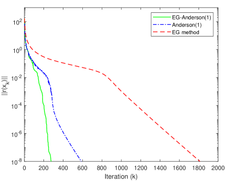
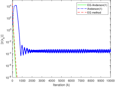
Example 4.1.
[20] Consider the Harker-Pang problem with linear mapping , where and
Here, is an matrix, is an skew-symmetric matrix and is an diagonal matrix with nonnegative diagonal entries. Therefore, it follows that is positive semidefinite. Let the feasible set be where . It is clear that is monotone and Lipschitz continuous.
We can easily obtain that the Lipschitz constant of is . Applying EG-Anderson(1) to this example, instead of using line search, we can do experiment with a constant stepsize that satisfies .
In the following experiments, we let , and every entry of the skew-symmetric matrix is uniformly generated from , and every diagonal entry of is uniformly generated from , and are randomly generated.
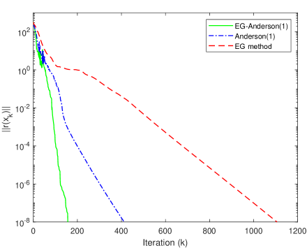
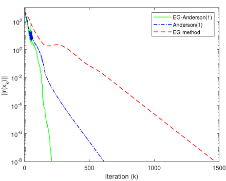
Figure 1 compares the decreasing on the residual function by EG-Anderson(1), Anderson(1) and EG algorithms at the same random initial point for Example 4.1 with and , respectively. For different dimension , Table 2 illustrates the average number of iterations and CPU time of the corresponding experiments at ten random initial points, where we see that the superiorities of EG-Anderson(1) over Anderson(1) and EG algorithms gradually emerges as the dimension increases.
| EG-Anderson(1) | Anderson(1) | EG | |||
|---|---|---|---|---|---|
| Sec.(avr) | 0.0032 | 0.0019 | 0.0042 | ||
| Iter.(avr) | 104.3 | 224.4 | 500.1 | ||
| Sec.(avr) | 0.0118 | 0.0155 | 0.0709 | ||
| Iter.(avr) | 161.9 | 418.6 | 1102.3 | ||
| Sec.(avr) | 0.0602 | 0.0892 | 0.3913 | ||
| Iter.(avr) | 204.9 | 549 | 1416.5 | ||
| Sec.(avr) | 0.6903 | 0.9482 | 4.6210 | ||
| Iter.(avr) | 216.7 | 596.3 | 1464.6 | ||
| Sec.(avr) | 5.0914 | 6.2813 | 31.7549 | ||
| Iter.(avr) | 244.9 | 604.2 | 1537.5 | ||
| Sec.(avr) | 20.5377 | 23.2472 | 140.8331 | ||
| Iter.(avr) | 247.1 | 545.1 | 1683.6 |
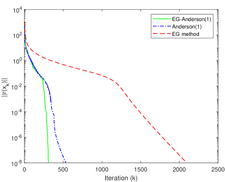
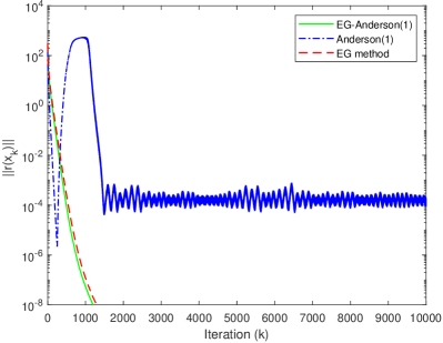
Example 4.2.
[35] Consider the quadratic fractional programming problem
with
where is the identity matrix, represents the vector that was defined in Example 4.1 and , , are randomly generated from a uniform distribution.
It is easily verified that and is positive definite, and consequently is pseudoconvex on . Thus, in can be written in the following explicit form:
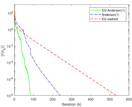
Let . Starting from the same random initial point, Figure 2 shows the comparisons of the results obtained by EG-Anderson(1), Anderson(1) and EG algorithms for Example 4.2 with and . Table 3 presents the average number of iterations and CPU time for the experiments with more cases on , conducted with ten different random initial points. Thus, the results indicate that EG-Anderson(1) outperforms both the Anderson(1) and EG algorithms across various dimensions in terms of iterations and CPU time.
| EG-Anderson(1) | Anderson(1) | EG | |||
|---|---|---|---|---|---|
| Sec.(avr) | 0.0073 | 0.0085 | 0.0288 | ||
| Iter.(avr) | 94.6 | 299.7 | 609 | ||
| Sec.(avr) | 0.1603 | 0.1790 | 0.8205 | ||
| Iter.(avr) | 91.9 | 238.5 | 531 | ||
| Sec.(avr) | 0.7249 | 0.9136 | 3.8403 | ||
| Iter.(avr) | 100.4 | 285.2 | 588.8 | ||
| Sec.(avr) | 2.7579 | 3.4896 | 14.3848 | ||
| Iter.(avr) | 98.4 | 285.3 | 576 | ||
| Sec.(avr) | 15.9044 | 19.5821 | 77.6780 | ||
| Iter.(avr) | 96.4 | 276 | 538 | ||
| Sec.(avr) | 59.7025 | 63.1694 | 275.2910 | ||
| Iter.(avr) | 106.1 | 262 | 556 |
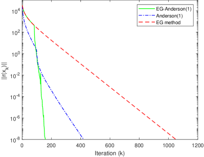
Example 4.3.
In numerical tests, we take , where matrices and vector are randomly generated as follows with an input integer :
From the above generation, we know that is a solution of (4.2).
In Figure 3, we present a comparative analysis of the outcomes achieved by applying EG-Anderson(1), Anderson(1) and EG algorithms to Example 4.3. All three methods in Figure 3 are initialized with the same random initial point. Table 4 summarizes the average number of iterations and CPU time for each method, where the corresponding experiments are repeated ten times with different random initial points.
In all dimensions, the average number of iterations and CPU time of EG-Anderson(1) are significantly less than those of Anderson(1) and EG algorithms. The advantages of EG-Anderson(1) become more pronounced as the dimension increases. For instance, in the case of , EG-Anderson(1) achieves an average number of iterations of 530.3 and an average CPU time of 84.5448 seconds, significantly outperforming Anderson(1) and EG algorithms.
| EG-Anderson(1) | Anderson(1) | EG | |||
|---|---|---|---|---|---|
| Sec.(avr) | 0.0038 | 0.0023 | 0.0088 | ||
| Iter.(avr) | 131.1 | 255.6 | 710.3 | ||
| Sec.(avr) | 0.0286 | 0.0298 | 0.1877 | ||
| Iter.(avr) | 256.6 | 557.8 | 1754.4 | ||
| Sec.(avr) | 0.3195 | 0.3335 | 1.9398 | ||
| Iter.(avr) | 234.8 | 509.2 | 1513.1 | ||
| Sec.(avr) | 2.0273 | 2.0347 | 13.3122 | ||
| Iter.(avr) | 320 | 639.8 | 2122.6 | ||
| Sec.(avr) | 18.9440 | 21.5331 | 169.6935 | ||
| Iter.(avr) | 462.1 | 1033.1 | 4146.3 | ||
| Sec.(avr) | 84.5448 | 92.3793 | 755.1626 | ||
| Iter.(avr) | 530.3 | 1176.7 | 4836.6 |
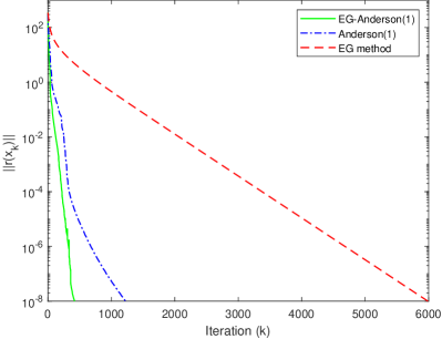
Example 4.4.
Consider the following partial differential equation (PDE) problem with free boundary
| (4.3) |
where , , , , and are unknown. Let . We choose
and
Then problem (4.3) has a solution as follows
Dividing the interval (0,1) into subintervals of equal width provides mesh points where
Using the five point finite difference method for the problem (4.3) at grid gives
and
Let and be the corresponding vectors transformed by and . Then, we obtain an NCP with
where is a block tri-diagonal positive definite matrix of dimension , and are both dimensional diagonal matrices with the diagonal elements being and respectively, and Note that the dimension of the corresponding complementarity problem is . Furthermore, the NCP can be equivalently formulated as with . We note that when in (4.3), the problem described in Example 4.4 reduces to the case outlined in Example 5.1 of [1].
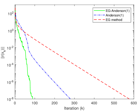
In the experiments, let . We set and , respectively. The effectiveness of EG-Anderson(1), Anderson(1) and EG algorithms for Example 4.4 with and is compared in Figure 4. All three methods are started from the same random initial point for each case.
As can be seen from Table 5, the average number of iterations for EG-Anderson(1) is consistently smaller than that of Anderson(1) and EG algorithms in all dimensions. Additionally, EG-Anderson(1) has a shorter CPU usage time, highlighting its higher computational efficiency. In high-dimensional problems, such as and , EG-Anderson(1) outperforms the other two algorithms in terms of the average number of iterations and CPU time, demonstrating higher efficiency and performance.
Similar to Table 5, Table 6 presents the average number of iterations and CPU time required for each algorithm in Example 4.4, but with a different value of (0.8 instead of 0.9).
| EG-Anderson(1) | Anderson(1) | EG | |||
|---|---|---|---|---|---|
| Sec.(avr) | 0.0059 | 0.0091 | 0.0336 | ||
| Iter.(avr) | 70.1 | 287.3 | 565 | ||
| Sec.(avr) | 0.0245 | 0.0315 | 0.1167 | ||
| Iter.(avr) | 123.6 | 358 | 713 | ||
| Sec.(avr) | 0.0450 | 0.0579 | 0.2401 | ||
| Iter.(avr) | 168.6 | 473.1 | 1050 | ||
| Sec.(avr) | 0.0788 | 0.1081 | 0.4866 | ||
| Iter.(avr) | 209.7 | 581.8 | 1404 | ||
| Sec.(avr) | 0.3410 | 0.4808 | 2.3559 | ||
| Iter.(avr) | 335.9 | 935.5 | 2378 | ||
| Sec.(avr) | 0.7649 | 0.9315 | 5.4866 | ||
| Iter.(avr) | 480.8 | 1162.2 | 3475 | ||
| Sec.(avr) | 1.0412 | 1.3647 | 7.6509 | ||
| Iter.(avr) | 563.5 | 1435.9 | 4260 |
| EG-Anderson(1) | Anderson(1) | EG | |||
|---|---|---|---|---|---|
| Sec.(avr) | 0.0225 | 0.0301 | 0.1583 | ||
| Iter.(avr) | 336.3 | 961.4 | 2798.5 | ||
| Sec.(avr) | 0.0885 | 0.1694 | 0.7814 | ||
| Iter.(avr) | 414.2 | 1756.5 | 5206.1 | ||
| Sec.(avr) | 0.1094 | 0.2149 | 1.3746 | ||
| Iter.(avr) | 422.7 | 1762.4 | 5988.2 | ||
| Sec.(avr) | 0.1541 | 0.2968 | 1.7913 | ||
| Iter.(avr) | 452.3 | 1684.7 | 5502.5 | ||
| Sec.(avr) | 0.5743 | 1.2679 | 8.5596 | ||
| Iter.(avr) | 546 | 2492.3 | 8737.9 | ||
| Sec.(avr) | 1.2120 | 2.6524 | |||
| Iter.(avr) | 748.8 | 3118.3 | |||
| Sec.(avr) | 1.7184 | 3.4303 | |||
| Iter.(avr) | 863.9 | 3309.9 |
5. Conclusions
This paper proposes an algorithm, called EG-Anderson(1) algorithm, for solving the pseudomonotone variational inequalities . This algorithm is based on EG method and Anderson acceleration. Firstly, the global sequence convergence of EG-Anderson(1) algorithm is proven without relying on the Lipschitz continuity and contractive condition that are required for the convergence analysis of EG method and Anderson acceleration in prior research. Moreover, when is locally Lipschitz continuous, the convergence rate of the residual function is analyzed and shown to be no worse than that of EG method. Finally, the effectiveness of EG-Anderson(1) algorithm has been validated through numerical experiments. The results demonstrate that it outperforms both Anderson(1) and EG algorithms in terms of the number of iterations and CPU time, especially in the context of solving Harker-Pang problem, fractional programming, nonlinear complementarity problem and PDE problem with free boundary.
References
- [1] G. Alefeld, X. Chen, A regularized projection method for complementarity problems with non-Lipschitzian functions, Math. Comput., 77 (2008): 379-395.
- [2] N. I. Alfredo, An iterative algorithm for the variational inequality problem, Comput. Appl. Math., 13 (1994): 103-114.
- [3] H. An, X. Jia, H. F. Walker, Anderson acceleration and application to the three-temperature energy equations, J. Comput. Phys., 347 (2017): 1-19.
- [4] D. G. Anderson, Iterative procedures for nonlinear integral equations, J. ACM, 12 (1965): 547-560.
- [5] H. Attouch, M. O. Czarnecki, J. Peypouquet, Coupling forward-backward with penalty schemes and parallel splitting for constrained variational inequalities, SIAM J. Optim., 21 (2011): 1251-1274.
- [6] V. Barbu, M. Rckner, Stochastic variational inequalities and applications to the total variation flow perturbed by linear multiplicative noise, Arch. Ration. Mech. Anal., 209 (2013): 797-834.
- [7] W. Bian, X. Chen, C. T. Kelley, Anderson acceleration for a class of nonsmooth fixed-point problems, SIAM J. Sci. Comput., 43 (2021): S1-S20.
- [8] R. I. Bot, E. R. Csetnek, P. T. Vuong, The Forward-Backward-Forward method from discrete and continuous perspective for pseudomonotone variational inequalities in Hilbert spaces, Eur. J. Oper. Res., 287 (2020): 49-56.
- [9] G. Cai, Q. L. Dong, Y. Peng, Strong convergence theorems for solving variational inequality problems with pseudomonotone and non-Lipschitz operators, J. Optim. Theory Appl., 188 (2021): 447-472.
- [10] Y. Censor, A. Gibali, S. Reich, Strong convergence of subgradient extragradient methods for the variational inequality problem in Hilbert space, Optim. Method Softw., 26 (2011): 827-845.
- [11] Y. Censor, A. Gibali, S. Reich, The subgradient extragradient method for solving variational inequalities in Hilbert space, J. Optim. Theory Appl., 148 (2011): 318-335.
- [12] X. Chen, C. T. Kelley, Convergence of the EDIIS algorithm for nonlinear equations, SIAM J. Sci. Comput., 41 (2019): A365-A379.
- [13] R. W. Cottle, J. C. Yao, Pseudo-monotone complementarity problems in Hilbert space, J. Optim. Theory Appl., 75 (1992): 281-295.
- [14] S. Dafermos, A. Nagurney, A network formulation of market equilibrium problems and variational inequalities, Oper. Res. Lett., 3 (1984): 247-250.
- [15] S. V. Denisov, V. V. Semenov, L. M. Chabak, Convergence of the modified extragradient method for variational inequalities with non-Lipschitz operators, Cybern. Syst. Anal., 51 (2015): 757-765.
- [16] F. Facchinei, J. S. Pang, Finite-dimensional variational inequalities and complementarity problems, New York: Springer-Verlag, 2003.
- [17] K. Goebel, S. Reich, Uniform Convexity, hperbolic geometry, and nonexpansive mappings, Marcel Dekker, New York, 1984.
- [18] A. A. Goldstein, Convex programming in Hilbert space, Bull. Amer. Math. Soc., 70 (1964): 709-710.
- [19] T. N. Hai, Two modified extragradient algorithms for solving variational inequalities, J. Glob. Optim., 78 (2020): 91-106.
- [20] P. T. Harker, J. S. Pang, For the linear complementarity problem, Lectures in Appl. Math., 26 (1990): 265-284.
- [21] C. Heinemann, K. Sturm, Shape optimization for a class of semilinear variational inequalities with applications to damage models, SIAM J. Math. Anal., 48 (2016): 3579-3617.
- [22] N. J. Higham, N. Strabi, Anderson acceleration of the alternating projections method for computing the nearest correlation matrix, Numer. Algorithms, 72 (2016): 1021-1042.
- [23] K. Huang, S. Zhang, An approximation-based regularized extra-gradient method for monotone variational inequalities, arXiv preprint arXiv:2210.04440, 2022.
- [24] K. Huang, S. Zhang, Beyond monotone variational inequalities: Solution methods and iteration complexities, arXiv preprint arXiv:2304.04153, 2023.
- [25] S. Karamardian, Complementarity problems over cones with monotone and pseudomonotone maps, J. Optim. Theory Appl., 18 (1976): 445-454.
- [26] S. Karamardian, S. Schaible, Seven kinds of monotone maps, J. Optim. Theory Appl., 66 (1990): 37-46.
- [27] G. M. Korpelevich, The extragradient method for finding saddle points and other problems, Ekon. Mat. Metody, 12 (1976): 747-756.
- [28] M. Lei, Y. He, An extragradient method for solving variational inequalities without monotonicity, J. Optim. Theory Appl., 188 (2021): 432-446.
- [29] P. E. Maing, A hybrid extragradient-viscosity method for monotone operators and fixed point problems, SIAM J. Control Optim., 47 (2008): 1499-1515.
- [30] Y. Malitsky, Projected reflected gradient methods for monotone variational inequalities, SIAM J. Optim., 25 (2015): 502-520.
- [31] Y. V. Malitsky, V.V. Semenov, An extragradient algorithm for monotone variational inequalities, Cybern. Syst. Anal., 50 (2014): 271-277.
- [32] J. Peypouquet, S. Sorin, Evolution equations for maximal monotone operators: asymptotic analysis in continuous and discrete time, J. Convex Anal., 17 (2010): 1113-1163.
- [33] R. T. Rockafellar, J. Sun, Solving Lagrangian variational inequalities with applications to stochastic programming, Math. Program., 181 (2020): 435-451.
- [34] M. V. Solodov, B. F. Svaiter, A hybrid approximate extragradient–proximal point algorithm using the enlargement of a maximal monotone operator, Set-Valued Anal., 7 (1999): 323-345.
- [35] D. V. Thong, V. T. Dung, P. K. Anh, H. Van Thang, A single projection algorithm with double inertial extrapolation steps for solving pseudomonotone variational inequalities in Hilbert space, J. Comput. Appl. Math., 426 (2023): 115099.
- [36] D. V. Thong, A. Gibali, Extragradient methods for solving non-Lipschitzian pseudomonotone variational inequalities, J. Fixed Point Theory Appl., 21 (2019): 1-19.
- [37] D. V. Thong, Y. Shehu, O. S. Iyiola, Weak and strong convergence theorems for solving pseudomonotone variational inequalities with non-Lipschitz mappings, Numer. Algorithms, 84 (2020): 795-823.
- [38] A. Toth, C. T. Kelley, Convergence analysis for Anderson acceleration, SIAM J. Numer. Anal., 53 (2015): 805-819.
- [39] P. T. Vuong, Y. Shehu, Convergence of an extragradient-type method for variational inequality with applications to optimal control problems, Numer. Algorithms, 81 (2019): 269-291.
- [40] W. Y. Wang, B. B. Ma, Extragradient type projection algorithm for solving quasimonotone variational inequalities, Optimization, (2023): 1-17.
- [41] J. Yang, H. Liu, A modified projected gradient method for monotone variational inequalities, J. Optim. Theory Appl., 179 (2018): 197-211.
- [42] J. Yang, H. Liu, Strong convergence result for solving monotone variational inequalities in Hilbert space, Numer. Algorithms, 80 (2019): 741-752.
- [43] J. Yang, H. Liu, Z. Liu, Modified subgradient extragradient algorithms for solving monotone variational inequalities, Optimization, 76 (2018): 2247-2258.
- [44] Y. Yao, O. S. Iyiola, Y. Shehu, Subgradient extragradient method with double inertial steps for variational inequalities, J. Sci. Comput., 90 (2022): 1-29.
- [45] M. Ye, Y. He, A double projection method for solving variational inequalities without monotonicity, Comput. Optim. Appl., 60 (2015): 141-150.
- [46] J. Zhang, B. O’Donoghue, S. Boyd, Globally convergent type-I Anderson acceleration for nonsmooth fixed-point iterations, SIAM J. Optim., 30 (2020): 3170-3197.
- [47] X. Zhang, W. Zhao, G. Zhou, W. Liu, An accelerated monotonic convergent algorithm for a class of non-Lipschitzian NCP(F) involving an M-matrix, J. Comput. Appl. Math., 397 (2021): 113624.