Deep Inertia Half-quadratic Splitting Unrolling Network for Sparse View CT Reconstruction
Abstract
Sparse view computed tomography (CT) reconstruction poses a challenging ill-posed inverse problem, necessitating effective regularization techniques. In this letter, we employ -norm () regularization to induce sparsity and introduce inertial steps, leading to the development of the inertial -norm half-quadratic splitting algorithm. We rigorously prove the convergence of this algorithm. Furthermore, we leverage deep learning to initialize the conjugate gradient method, resulting in a deep unrolling network with theoretical guarantees. Our extensive numerical experiments demonstrate that our proposed algorithm surpasses existing methods, particularly excelling in fewer scanned views and complex noise conditions.
Index Terms:
-norm, inertial, wavelet, unrolling, Sparse ViewI Introduction
Computed tomography (CT) is crucial in modern medicine. However, the ionizing radiation from X-rays has led to interest in low-dose CT. Sparse view CT is an innovative approach that reduces projection data, thereby minimizing radiation and shortening scan times. However, it can cause image degradation, including streak artifacts [1]. Mathematically, the CT image reconstruction problem model can be succinctly described as follows:
| (1) |
where is the measured low quality image, is the measurement operator, is the original high quality image, and is the noise. In fact, in incomplete data CT reconstruction, the matrix is noninvertible. Hence, the inverse problem (1) is ill-posed.
Classical CT reconstruction techniques, such as Algebraic Reconstruction Techniques (ART) [2] and Filtered Backprojection (FBP) [3, 4], struggle to effectively handle sparse view CT. To address this, numerous algorithms have been proposed, with regularization models gaining widespread use. These models typically take the following form:
| (2) |
where represents the regularization term, and the weighted parameter balances the data fidelity and regularization terms. Various regularization terms, such as BM3D [5, 6, 7], total variation [8], sparsity [9, 10], low rank [11], and wavelets [12, 13, 14], have been employed to tackle this challenge.
With the advent of deep learning in image processing, an increasing number of sparse view CT reconstructions are leveraging deep learning algorithms to achieve superior performance. These primarily include direct reconstruction using end-to-end network structures [15, 16], and deep unrolling combined with traditional algorithms [17, 13, 18, 19, 20]. The advantage of deep unfolding networks is that they are driven by both model and data [21], meaning that prior knowledge in the domain can assist in learning. Recently, there are new techniques introduced to deep learning, such as attention mechanisms [22], and diffusion models [23, 24, 25], etc. Currently, state-of-the-art sparse-view CT reconstruction results are obtained by score-based model [26] and diffusion model [27]. While deep learning algorithms offer improved performance, they are dependent on high-quality pairwise data and lack theoretical guarantees, rendering them as black-box algorithms.
In this letter, we address the sparse view CT reconstruction problem by leveraging the superior sparsity of the -norm () in conjunction with wavelet transform. To tackle this non-convex and non-continuous problem, we introduce the Inertial -norm Half-Quadratic Splitting method (IHQSp), which employs inertial steps to expedite convergence. We establish the convergence of the IHQSp algorithm. During the CT image reconstruction, the corresponding subproblem is resolved using the conjugate gradient (CG) method. Considering the n-step quadratic convergence of CG, we propose using a network trained via deep learning as the initializer for CG. In the context of the IHQSp algorithm, the network solely provides the initial value for the CG, thereby not influencing the algorithm’s convergence. From a deep learning perspective, we derive a learning algorithm IHQSp-Net with convergence guarantees, which is deep unrolled by the IHQSp algorithm. We validate our proposed IHQSp-CG and IHQSp-Net through extensive numerical experiments on two datasets, demonstrating their exceptional performance.
II Inertial HQSp-CG Algorithm and Convergence Analysis
II-A Inertial HQSp-CG Algorithm
In order to take advantage of the sparsity of the CT image, we use the -norm with the wavelet transform to form the regularization term in (2), i.e.
| (3) |
where , is a -channel operator with . The operator is chosen as the highpass components of the piecewise linear tight wavelet frame transform [28]. Solving (3) directly is challenging due to the discontinuity in the norm. To solve (3), we introduce the auxiliary variable , and use the half-quadratic splitting method to obtain the following problem:
| (4) |
where and with are weight parameters. The above problem can be split into -subproblem and -subproblem solved in alternating iterations. To speed up the convergence, inspired by the inertia algorithm [29, 30], we introduce inertia steps in solving the two subproblems, i.e.,
| (5) | ||||
| (6) | ||||
| (7) | ||||
| (8) |
where (5) and (7) are subproblem solving steps, (6) and (8) are inertia steps, and and are inertia weight parameters.
The -update step (5) can be solved by the proximal operator , which is defined as
| (9) |
where , it can be computed as [31]
| (10) |
where , , is the solution of over the region . Since is convex, when , can be efficiently solved using Newton’s method.
For the -update step (7), according to the Euler-Lagrange equations, we have:
To avoid the inverse, this equation can be solved using the conjugate gradient method. We call our algorithm as Inertial HQSp-CG (IHQSp-CG) for short and summarized in Algorithm 1. Next, we establish the global convergence of the IHQSp-CG algorithm.
 |
 |
II-B Convergence analysis
In this section, we provide a convergence analysis of Algorithm 1.
Lemma II.1.
Suppose that the sequences and generated via Algorithm 1, , then the sets and are bounded.
Theorem II.1.
Let and be the sequences generated by our algorithm. Then any cluster point of is the global minimum point of .
Details of the proof can be found in the supplementary material.
| Data | AAPM Dataset | ||||||||||
|---|---|---|---|---|---|---|---|---|---|---|---|
| Method | Traditional algorithm | Deep learning algorithm | |||||||||
| Method | FBP | BM3D | HQS-CG | HQSp-CG | PWLS-CSCGR | IHQSp-CG | PDNet | FBPNet | MetaInvNet | IHQSp-Net* | IHQSp-Net |
| Noise | |||||||||||
| 180 | 23.64/0.5136 | 24.82/0.6839 | 31.65/0.8047 | 32.10/0.8131 | 26.72/24.7975 | 32.16/0.8138 | 30.06/0.8124 | 31.73/0.8138 | 33.01/0.8348 | 32.70/0.8297 | 33.18/ 0.8415 |
| 120 | 20.69/0.4104 | 23.31/0.6454 | 30.11/0.7659 | 30.72/0.7841 | 26.97/23.9243 | 30.86/0.7865 | 28.89/0.7813 | 30.36/0.7811 | 32.17/0.8103 | 31.45/0.7999 | 32.08/ 0.8148 |
| 90 | 20.11/0.3494 | 23.55/0.6143 | 28.83/0.7324 | 29.59/0.7602 | 25.76/22.8060 | 29.81/0.7647 | 28.26/0.7633 | 29.60/0.7674 | 31.56/0.7939 | 30.47/0.7777 | 31.66/ 0.8032 |
| 60 | 18.21/0.2762 | 22.34/0.5580 | 26.84/0.6809 | 27.79/0.7226 | 23.94/21.0367 | 28.06/0.7298 | 26.61/0.7298 | 28.06/0.7397 | 30.38/0.7627 | 28.89/0.7399 | 30.24/ 0.7671 |
| Noise | and | ||||||||||
| 180 | 22.77/0.4397 | 24.82/0.6830 | 30.57/0.7641 | 30.91/0.7845 | 25.98/22.0973 | 30.92/0.7858 | 29.54/0.7922 | 31.38/0.7990 | 32.02/0.8080 | 31.53/0.8005 | 32.25/ 0.8157 |
| 120 | 20.04/0.3494 | 23.31/0.6443 | 29.08/0.7179 | 29.81/0.7595 | 22.45/14.5781 | 29.90/0.7619 | 28.17/0.7633 | 30.15/0.7750 | 31.33/0.7929 | 30.48/0.7743 | 31.40/ 0.7961 |
| 90 | 19.37/0.2968 | 23.55/0.6132 | 27.91/0.6832 | 28.78/0.7369 | 22.94/15.7751 | 28.97/0.7430 | 27.16/0.7363 | 29.19/0.7570 | 30.76/0.7674 | 29.71/0.7516 | 30.98/ 0.7815 |
| 60 | 17.55/0.2341 | 22.37/0.5575 | 26.18/0.6359 | 27.09/0.6961 | 22.63/16.3278 | 27.30/0.7049 | 25.51/0.7077 | 28.13/0.7332 | 29.66/0.7424 | 28.62/0.7213 | 30.08/ 0.7597 |
| Data | Covid-19 Dataset | ||||||||||
| Method | FBP | BM3D | HQS-CG | HQSp-CG | PWLS-CSCGR | IHQSp-CG | PDNet | FBPNet | MetaInvNet | IHQSp-Net* | IHQSp-Net |
| Noise | |||||||||||
| 180 | 23.91/0.5361 | 25.46/0.7304 | 33.32/0.8393 | 33.93/0.8496 | 28.50/20.5285 | 34.05/0.8515 | 30.71/0.8413 | 33.21/0.8512 | 34.76/0.8638 | 34.43/0.8584 | 35.03/ 0.8704 |
| 120 | 21.07/0.4303 | 24.19/0.6906 | 31.56/0.8041 | 32.29/0.8241 | 28.25/19.7033 | 32.64/0.8285 | 29.61/0.8140 | 31.66/0.8196 | 34.06/ 0.8523 | 32.95/0.8290 | 33.83/0.8489 |
| 90 | 20.50/0.3665 | 24.11/0.6585 | 29.91/0.7707 | 30.83/0.8015 | 27.01/19.1825 | 31.29/0.8078 | 29.12/0.7980 | 30.81/0.8074 | 33.25/0.8380 | 31.93/0.8120 | 33.52/ 0.8432 |
| 60 | 18.47/0.2897 | 22.26/0.5966 | 27.30/0.7179 | 28.36/0.7621 | 24.98/17.8874 | 28.94/0.7731 | 27.34/0.7651 | 28.36/0.7740 | 31.88/ 0.8150 | 30.12/0.7729 | 31.81/0.8147 |
| Noise | and | ||||||||||
| 180 | 22.96/0.4426 | 25.45/0.7294 | 31.81/0.7919 | 32.30/0.8163 | 27.44/17.9762 | 32.34/0.8188 | 30.13/0.8199 | 32.84/0.8367 | 33.69/0.8452 | 32.75/0.8250 | 33.98/ 0.8482 |
| 120 | 20.32/0.3515 | 24.18/0.6893 | 30.17/0.7480 | 31.10/0.7967 | 22.97/11.6984 | 31.33/0.8009 | 29.35/0.7979 | 31.45/0.8154 | 32.87/0.8302 | 31.65/0.7993 | 33.06/ 0.8326 |
| 90 | 19.65/0.2980 | 24.10/0.6572 | 28.78/0.7147 | 29.81/0.7748 | 23.63/13.0201 | 30.21/0.7832 | 27.78/0.7682 | 30.45/0.7979 | 32.18/0.8150 | 30.79/0.7787 | 32.63/ 0.8239 |
| 60 | 17.71/0.2340 | 22.27/0.5956 | 26.58/0.6674 | 27.60/0.7328 | 23.41/13.8117 | 28.05/0.7444 | 26.25/0.7414 | 28.80/0.7729 | 30.80/0.7897 | 29.39/0.7493 | 31.62/ 0.8048 |
| Cpu (s) | 0.99 | 3.45 | 18.63 | 34.72 | – | 26.24 | 2.03 | 5.18 | 6.76 | 2.08 | 6.98 |
| Gpu (s) | – | – | 8.86 | 17.63 | 1530.59 | 15.91 | 0.62 | 1.35 | 1.92 | 1.98 | 2.29 |
III Conjugate gradient initialization and deep unrolling networks
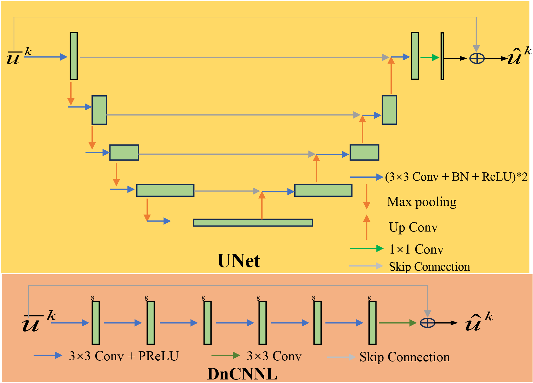
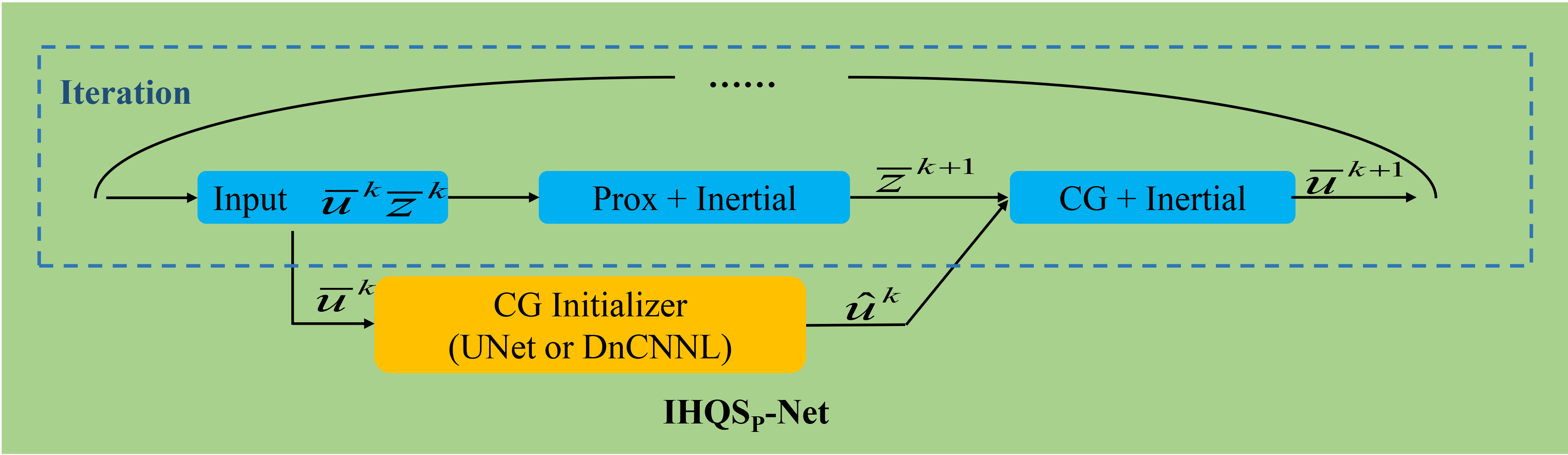
The algorithm, as per Algorithm 1, is divided into two subproblems: z-subproblem for denoising and u-subproblem for CT image reconstruction. The u-subproblem solution uses the conjugate gradient method, known for its super-linear convergence rate. The convergence speed is tied to the spectral distribution of the coefficient matrix, with faster convergence when eigenvalues are concentrated and the condition number is smaller [32, 33]. A well-defined initial value can lead to finite iterations for convergence. To facilitate this, we introduce a deep learning network to adjust the input at each iteration:
where represents the learnable network parameter, and is the corrected result. The algorithm’s structure can incorporate any network structure, with UNet and lightweight DnCNN as examples, referred to as IHQSp-Net and IHQSp-Net*, respectively. A detailed description is shown in Fig. 1. The parameter is trained through a loss function:
where and are weight factors, we set . is the loss, i.e. . is the structural similarity loss, i.e. [34].
From an algorithmic view, the deep network is embedded in the splitting algorithm, serving as an initializer for CG solving without affecting convergence. From a deep learning view, the splitting algorithm framework is a deep unrolling network with theoretical guarantees. The integration of both enhances performance while ensuring theoretical robustness.
IV Numerical experiments
IV-A Datasets and experimental settings
The deep learning algorithm used training and validation data from the “2016 NIH-AAPM-Mayo Clinic Low Dose CT Grand Challenge” dataset [35]. The training set had 1596 slices from five patients, and the validation set had 287 slices from one patient. Experiments were uniformly performed using a fan beam geometry with 800 detector elements. The test data included 38 slices from new patients in the AAPM dataset and 30 slices from the Covid-19 dataset [36] to assess the algorithm’s generalization and robustness.
Our proposed algorithms were compared with eight others, including five traditional (FBP [3], BM3D [5], HQS-CG [13], combining compressed sensing and sparse convolutional coding for PWLS-CSCGR [10], HQSp-CG without inertial norms) and three deep learning algorithms (PDNet [17], FBPNet [15], MetaInvNet [13]). For our lightweight IHQSp-Net* and IHQSp-Net, we set K = 6 and limited the CG algorithm iterations to 7. Data were degraded with different angles (60, 90, 120, 180) and two noise levels (Gaussian noise , mixed Gaussian and Poisson noise with intensity ).
Our models were implemented using the PyTorch framework. The experiments were conducted on PyTorch 1.3.1 backend with an NVIDIA Tesla V100S GPU, 8-core CPU and 32GB RAM. For IHQSp-CG, the hyperparameters were set to , , , . For IHQSp-Net, the hyperparameters were set to , , , .
 |
 |
 |
 |
 |
 |
| (a) Ground truth | (b) FBP | (c) BM3D | (d) HQS-CG | (e) HQSp-CG | (f) PWLS-CSCGR |
 |
 |
 |
 |
 |
 |
| (g) IHQSp-CG | (h) PDNet | (i) FBPNet | (j) MetaInvNet | (k) IHQSp-Net* | (l) IHQSp-Net |
 |
 |
IV-B Comparison of quantitative and qualitative results
Evaluation metrics used are peak signal-to-noise ratio (PSNR) [37] and structural similarity (SSIM) [34]. For a comprehensive evaluation of the algorithm performance, we added a comparison of the mean absolute error (MAE) and the root mean square error (RMSE) in the supplementary material. Table I shows that our proposed IHQSp-CG algorithm outperforms other traditional algorithms, even surpassing the deep learning algorithms PDNet and FBPNet on both AAPM and Covid-19 datasets. It shows greater robustness to noise and missing range than the HQS-CG algorithm, with an average improvement of more than 0.5 dB for 180-degree and 120-degree observations, and over 1 dB for 90-degree and 60-degree observations.
Our proposed IHQSp-Net outperforms other deep learning methods, especially in handling mixed noises. Our lightweight IHQSp-Net* significantly improves upon the traditional IHQSp-CG, indicating a lightweight CG initializer can enhance performance and convergence speed. Compared to FBPNet, IHQSp-Net shows an average improvement of 2 dB, highlighting the benefits of integrating traditional algorithms with theoretical guarantees into deep networks. Meanwhile, Table I gives the running time for each algorithm to reconstruct a 512512 observation of 90 degrees.
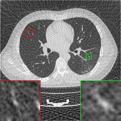
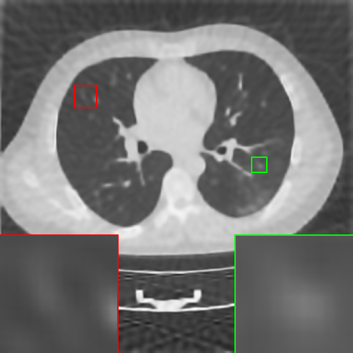
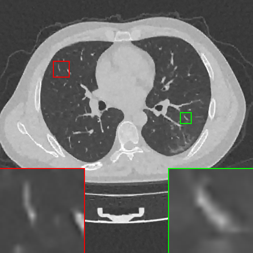
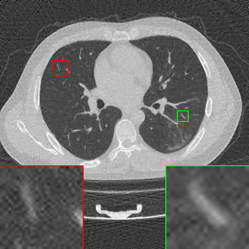
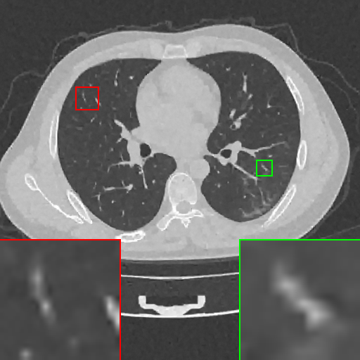
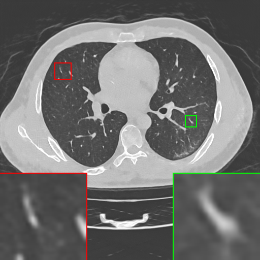
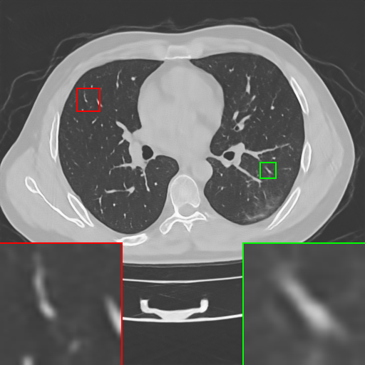
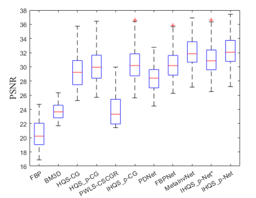
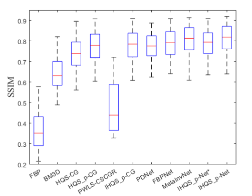
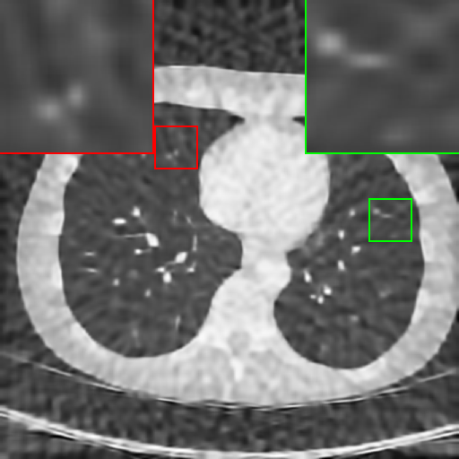
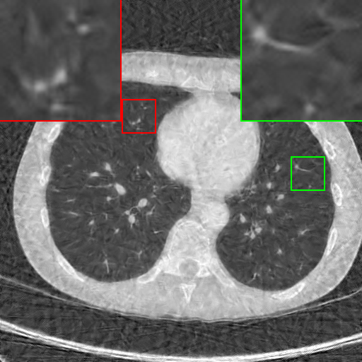
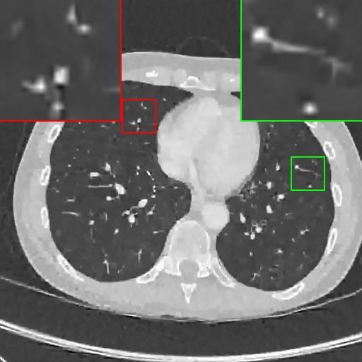
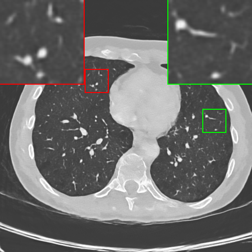
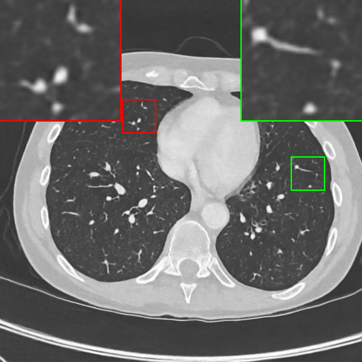
Fig. 2 compares reconstructed images. FBP, BM3D, and HQS-CG show artifacts and missing structures due to lack of observation angle. Our IHQSp-CG yields smoother results. Deep learning algorithms like PDNet and FBPNet produce smooth but over-smoothed results, blurring structural information. Both MetaInvNet and our IHQSp-Net produce pleasing results, but IHQSp-Net captures more details and avoids pseudo-connections seen in MetaInvNet. Notably, IHQSp-Net* visually outperforms IHQSp-CG, highlighting the importance of the CG initializer. The robustness analysis of all the algorithms is given in Fig. 3. By statistically analyzing the reconstructed images for all noise cases, observation angle cases and datasets, it can be found that the proposed IHQSp-CG and IHQSp-Net are robust to noise, observation angle, and data.
 |
 |
| (a) | (b) Convergence |
IV-C Ablation experiment
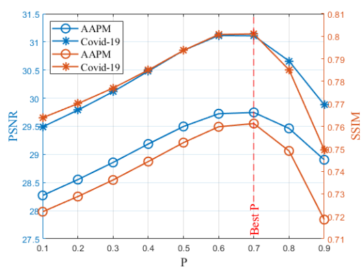
There is a key parameter in IHQSp which controls the sparsity of the regular term. Different values of affect the reconstruction results of CT images [9]. Therefore, we need to discuss the different -value effects. Fig. 4(a) shows the results of different values on two datasets, AAPM and Covid-19. From the figure, we can find that between 1 and 0.7, the reconstruction effect is enhanced as decreases. This reflects the advantage of the paradigm over . However, lower is not better. As can be seen in the figure, for IHQSp, the optimal .
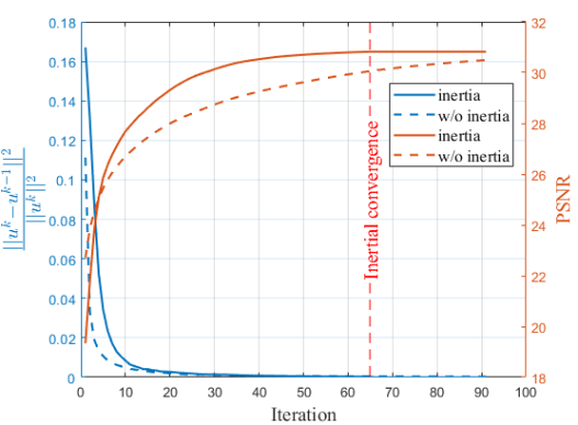
One of the contributions of IHQSp is the introduction of inertial steps to accelerate the convergence of HQS. HQSp-CG, in Table I, shows the numerical results without inertia step. It can be found that the introduction of the inertia step can effectively improve the algorithm’s performance, and the improvement becomes more obvious as the observation angle becomes sparser. Fig. 4(b) gives a comparison between IHQSp and HQSp-CG for iterative reconstruction when the 90-degree observation is corrupted by mixed Gaussian Poisson noise. PSNR and error are used as metrics. From Fig. 4(b), IHQSp stops iterating at step 65, while HQSp without inertial steps iterates until step 90. Meanwhile, HQSp with more iterations does not outperform IHQSp in PSNR. This reflects the importance of introducing inertial steps.
V Conclusion
We propose an inertial -norm half-quadratic splitting algorithm for sparse view CT image reconstruction and establish its convergence. Building on IHQSp, we introduce IHQSp-Net, a deep unrolling network that comes with theoretical guarantees. Both quantitative and qualitative comparisons with other methods demonstrate that our proposed IHQSp-CG and IHQSp-Net outperform in terms of performance and robustness, particularly excelling in scenarios with fewer scanned views and complex noise situations.
References
- [1] J. Bian, J. H. Siewerdsen, X. Han, E. Y. Sidky, J. L. Prince, C. A. Pelizzari, and X. Pan, “Evaluation of sparse-view reconstruction from flat-panel-detector cone-beam ct,” Phys. Med. Biol., vol. 55, no. 22, p. 6575, 2010.
- [2] R. Gordon, R. Bender, and G. T. Herman, “Algebraic reconstruction techniques (art) for three-dimensional electron microscopy and x-ray photography,” J. Theor. Biol., vol. 29, no. 3, pp. 471–481, 1970.
- [3] A. Katsevich, “Theoretically exact filtered backprojection-type inversion algorithm for spiral ct,” SIAM J. Appl. Math., vol. 62, no. 6, pp. 2012–2026, 2002.
- [4] Y. Wei, G. Wang, and J. Hsieh, “Relation between the filtered backprojection algorithm and the backprojection algorithm in ct,” IEEE Signal Process. Lett., vol. 12, no. 9, pp. 633–636, 2005.
- [5] K. Dabov, A. Foi, V. Katkovnik, and K. Egiazarian, “Image denoising by sparse 3-d transform-domain collaborative filtering,” IEEE Trans. Image Process., vol. 16, no. 8, pp. 2080–2095, 2007.
- [6] T. Zhao, J. Hoffman, M. McNitt-Gray, and D. Ruan, “Ultra-low-dose ct image denoising using modified bm3d scheme tailored to data statistics,” Med. Phys., vol. 46, no. 1, pp. 190–198, 2019.
- [7] Y. Guo, A. Davy, G. Facciolo, J.-M. Morel, and Q. Jin, “Fast, nonlocal and neural: a lightweight high quality solution to image denoising,” IEEE Signal Process. Lett., vol. 28, pp. 1515–1519, 2021.
- [8] F. Mahmood, N. Shahid, U. Skoglund, and P. Vandergheynst, “Adaptive graph-based total variation for tomographic reconstructions,” IEEE Signal Process. Lett., vol. 25, no. 5, pp. 700–704, 2018.
- [9] L. Zhang, H. Zhao, W. Ma, J. Jiang, L. Zhang, J. Li, F. Gao, and Z. Zhou, “Resolution and noise performance of sparse view x-ray ct reconstruction via lp-norm regularization,” Phys. Medica, vol. 52, pp. 72–80, 2018.
- [10] P. Bao, W. Xia, K. Yang, W. Chen, M. Chen, Y. Xi, S. Niu, J. Zhou, H. Zhang, H. Sun, Z. Wang, and Y. Zhang, “Convolutional sparse coding for compressed sensing ct reconstruction,” IEEE Trans. Med. Imaging, vol. 38, no. 11, pp. 2607–2619, 2019.
- [11] K. Kim, J. C. Ye, W. Worstell, J. Ouyang, Y. Rakvongthai, G. El Fakhri, and Q. Li, “Sparse-view spectral ct reconstruction using spectral patch-based low-rank penalty,” IEEE Trans. Med. Imaging, vol. 34, no. 3, pp. 748–760, 2014.
- [12] B. Dong, J. Li, and Z. Shen, “X-ray ct image reconstruction via wavelet frame based regularization and radon domain inpainting,” J. Sci. Comput., vol. 54, no. 2, pp. 333–349, 2013.
- [13] H. Zhang, B. Liu, H. Yu, and B. Dong, “Metainv-net: meta inversion network for sparse view ct image reconstruction,” IEEE Trans. Med. Imaging, vol. 40, no. 2, pp. 621–634, 2020.
- [14] E. Sakhaee and A. Entezari, “Joint inverse problems for signal reconstruction via dictionary splitting,” IEEE Signal Process. Lett., vol. 24, no. 8, pp. 1203–1207, 2017.
- [15] K. H. Jin, M. T. McCann, E. Froustey, and M. Unser, “Deep convolutional neural network for inverse problems in imaging,” IEEE Trans. Image Process., vol. 26, no. 9, pp. 4509–4522, 2017.
- [16] W. Du, H. Chen, P. Liao, H. Yang, G. Wang, and Y. Zhang, “Visual attention network for low-dose ct,” IEEE Signal Process. Lett., vol. 26, no. 8, pp. 1152–1156, 2019.
- [17] J. Adler and O. Öktem, “Learned primal-dual reconstruction,” IEEE Trans. Med. Imaging, vol. 37, no. 6, pp. 1322–1332, 2018.
- [18] B. Shi, K. Jiang, S. Zhang, Q. Lian, Y. Qin, and Y. Zhao, “Mud-net: multi-domain deep unrolling network for simultaneous sparse-view and metal artifact reduction in computed tomography,” Machine Learning: Science and Technology, vol. 5, no. 1, p. 015010, 2024.
- [19] J. Pan, H. Yu, Z. Gao, S. Wang, H. Zhang, and W. Wu, “Iterative residual optimization network for limited-angle tomographic reconstruction,” IEEE Trans. Image Process., vol. 33, pp. 910–925, 2024.
- [20] W. Wu, D. Hu, C. Niu, H. Yu, V. Vardhanabhuti, and G. Wang, “Drone: Dual-domain residual-based optimization network for sparse-view ct reconstruction,” IEEE Trans. Med. Imaging, vol. 40, no. 11, pp. 3002–3014, 2021.
- [21] B. Shi, S. Zhang, K. Jiang, and Q. Lian, “Coupling model- and data-driven networks for ct metal artifact reduction,” IEEE Trans. Comput. Imaging, vol. 10, pp. 415–428, 2024.
- [22] W. Wu, X. Guo, Y. Chen, S. Wang, and J. Chen, “Deep embedding-attention-refinement for sparse-view ct reconstruction,” IEEE Trans. Instrum. Meas., vol. 72, pp. 1–11, 2023.
- [23] W. Wu, Y. Wang, Q. Liu, G. Wang, and J. Zhang, “Wavelet-improved score-based generative model for medical imaging,” IEEE Trans. Med. Imaging, vol. 43, no. 3, pp. 966–979, 2024.
- [24] K. Xu, S. Lu, B. Huang, W. Wu, and Q. Liu, “Stage-by-stage wavelet optimization refinement diffusion model for sparse-view ct reconstruction,” IEEE Trans. Med. Imaging, pp. 1–1, 2024.
- [25] W. Wu, J. Pan, Y. Wang, S. Wang, and J. Zhang, “Multi-channel optimization generative model for stable ultra-sparse-view ct reconstruction,” IEEE Trans. Med. Imaging, pp. 1–1, 2024.
- [26] Y. Wang, Z. Li, and W. Wu, “Time-reversion fast-sampling score-based model for limited-angle ct reconstruction,” IEEE Trans. Med. Imaging, pp. 1–1, 2024.
- [27] Z. Li, D. Chang, Z. Zhang, F. Luo, Q. Liu, J. Zhang, G. Yang, and W. Wu, “Dual-domain collaborative diffusion sampling for multi-source stationary computed tomography reconstruction,” IEEE Trans. Med. Imaging, pp. 1–1, 2024.
- [28] A. Ron and Z. Shen, “Affine systems inl2 (rd): the analysis of the analysis operator,” J. Funct. Anal., vol. 148, no. 2, pp. 408–447, 1997.
- [29] F. Alvarez and H. Attouch, “An inertial proximal method for maximal monotone operators via discretization of a nonlinear oscillator with damping,” Set-Valued Anal., vol. 9, pp. 3–11, 2001.
- [30] P. Ochs, Y. Chen, T. Brox, and T. Pock, “ipiano: Inertial proximal algorithm for nonconvex optimization,” SIAM J. Imaging Sci., vol. 7, no. 2, pp. 1388–1419, 2014.
- [31] G. Marjanovic and V. Solo, “On optimization and matrix completion,” IEEE Trans. Signal Process., vol. 60, no. 11, pp. 5714–5724, 2012.
- [32] D. Smyl, T. N. Tallman, D. Liu, and A. Hauptmann, “An efficient quasi-newton method for nonlinear inverse problems via learned singular values,” IEEE Signal Process. Lett., vol. 28, pp. 748–752, 2021.
- [33] M. Savanier, E. Chouzenoux, J.-C. Pesquet, and C. Riddell, “Unmatched preconditioning of the proximal gradient algorithm,” IEEE Signal Process. Lett., vol. 29, pp. 1122–1126, 2022.
- [34] Z. Wang, A. C. Bovik, H. R. Sheikh, and E. P. Simoncelli, “Image quality assessment: from error visibility to structural similarity,” IEEE Trans. Image Process., vol. 13, no. 4, pp. 600–612, 2004.
- [35] C. McCollough, “Tu-fg-207a-04: overview of the low dose ct grand challenge,” Med. Phys., vol. 43, no. 6Part35, pp. 3759–3760, 2016.
- [36] Y. Shi, G. Wang, X.-p. Cai, J.-w. Deng, L. Zheng, H.-h. Zhu, M. Zheng, B. Yang, and Z. Chen, “An overview of covid-19,” J. Zhejiang Univ.-SCI. B, vol. 21, no. 5, pp. 343–360, 2020.
- [37] A. Hore and D. Ziou, “Image quality metrics: Psnr vs. ssim,” in Proc. IEEE Conf. Comput. Vision Pattern Recognit. (CVPR). IEEE, 2010, pp. 2366–2369.
VI Convergence analysis
Define ,
Lemma VI.1.
Suppose that the sequences and generated via Algorithm 1, , then the sets and are bounded.
Proof.
In our problem, represents the gray value of an image, i.e., , therefore is bounded. From the -update step (7), we have
which together with and is the given wavelet transform operator, yields,
From is bounded, it is easy to see that is bounded.
On the other hand, from (8), we find
| (11) | ||||
Since is bounded, there exists a constant such that , . If holds, then . It follows from (11) that
which consequently results in the boundedness of sequence . By (6), we have . Thus, is bounded because is bounded. Therefore, for , we get and are bounded. ∎
| Data | AAPM Dataset | ||||||||||
| Method | Traditional algorithm | Deep learning algorithm | |||||||||
| Method | FBP | BM3D | HQS-CG | HQSp-CG | PWLS-CSCGR | IHQSp-CG | PDNet | FBPNet | MetaInvNet | IHQSp-Net* | IHQSp-Net |
| Noise | |||||||||||
| 180 | 13.18/16.79 | 10.61/14.66 | 4.73/6.74 | 4.51/6.41 | 7.98/453.28 | 4.48/6.37 | 5.69/8.07 | 4.74/6.67 | 4.17/5.79 | 4.29/5.99 | 4.07/ 5.68 |
| 120 | 17.45/23.56 | 11.97/17.45 | 5.51/8.01 | 5.10/7.48 | 8.06/438.85 | 5.03/7.37 | 6.33/9.22 | 5.34/7.78 | 4.52/ 6.37 | 4.83/6.89 | 4.54/6.42 |
| 90 | 19.63/25.21 | 12.24/16.96 | 6.25/9.26 | 5.62/8.50 | 9.12/503.83 | 5.50/8.29 | 6.57/9.90 | 5.76/8.48 | 4.78/6.82 | 5.28/7.69 | 4.70/ 6.74 |
| 60 | 24.54/31.38 | 14.36/19.48 | 7.61/11.62 | 6.57/10.43 | 11.07/619.98 | 6.36/10.11 | 7.56/11.94 | 6.48/10.12 | 5.37/ 7.79 | 6.08/9.20 | 5.45/7.90 |
| Noise | and | ||||||||||
| 180 | 14.61/18.54 | 10.61/14.67 | 5.45/7.61 | 5.14/7.31 | 9.04/491.19 | 5.13/7.32 | 6.01/8.56 | 4.88/6.94 | 4.58/6.48 | 4.86/6.83 | 4.47/ 6.30 |
| 120 | 19.14/25.41 | 11.98/17.45 | 6.35/9.01 | 5.64/8.29 | 14.26/731.87 | 5.58/8.22 | 6.84/10.00 | 5.48/7.97 | 4.84/6.99 | 5.37/7.69 | 4.85/ 6.94 |
| 90 | 21.53/27.43 | 12.24/16.96 | 7.12/10.28 | 6.16/9.32 | 13.22/692.11 | 6.02/9.12 | 7.37/11.23 | 6.01/8.90 | 5.19/7.46 | 5.78/8.38 | 5.05/ 7.26 |
| 60 | 26.72/33.85 | 14.30/19.43 | 8.44/12.54 | 7.19/11.31 | 13.36/718.63 | 6.97/11.04 | 8.32/13.56 | 6.43/10.03 | 5.71/8.44 | 6.37/9.50 | 5.47/ 8.05 |
| Data | Covid-19 Dataset | ||||||||||
| Method | FBP | BM3D | HQS-CG | HQSp-CG | PWLS-CSCGR | IHQSp-CG | PDNet | FBPNet | MetaInvNet | IHQSp-Net* | IHQSp-Net |
| Noise | |||||||||||
| 180 | 12.88/16.26 | 10.49/13.64 | 4.03/5.62 | 3.77/5.27 | 6.86/289.66 | 3.73/5.19 | 5.50/7.50 | 4.14/5.68 | 3.54/4.78 | 3.65/4.97 | 3.42/ 4.65 |
| 120 | 16.75/22.56 | 11.69/15.79 | 4.75/6.84 | 4.33/6.32 | 7.16/296.62 | 4.21/6.07 | 6.06/8.50 | 4.75/6.76 | 3.77/ 5.19 | 4.19/5.85 | 3.85/5.32 |
| 90 | 18.60/24.11 | 12.01/15.91 | 5.51/8.23 | 4.86/7.44 | 7.99/342.59 | 4.69/7.06 | 6.15/8.99 | 5.15/7.46 | 4.04/5.69 | 4.58/6.57 | 3.94/ 5.52 |
| 60 | 23.30/30.45 | 14.40/19.70 | 6.98/11.05 | 5.93/9.81 | 9.81/432.80 | 5.61/9.19 | 7.08/11.03 | 6.13/9.80 | 4.54/ 6.62 | 5.41/8.06 | 4.57/6.66 |
| Noise | and | ||||||||||
| 180 | 14.35/18.14 | 10.49/13.65 | 4.84/6.63 | 4.47/6.29 | 8.07/326.25 | 4.44/6.26 | 5.87/8.04 | 4.28/5.94 | 3.87/5.40 | 4.32/5.99 | 3.80/ 5.24 |
| 120 | 18.59/24.58 | 11.70/15.81 | 5.68/7.98 | 4.92/7.20 | 13.59/544.19 | 4.82/7.02 | 6.23/8.80 | 4.88/6.94 | 4.18/5.92 | 4.80/6.78 | 4.14/ 5.80 |
| 90 | 20.72/26.58 | 12.01/15.93 | 6.45/9.35 | 5.44/8.33 | 12.32/504.26 | 5.25/7.97 | 7.08/10.47 | 5.26/7.76 | 4.46/6.39 | 5.22/7.47 | 4.30/ 6.09 |
| 60 | 25.79/33.21 | 14.37/19.68 | 7.84/12.00 | 6.57/10.68 | 12.22/517.15 | 6.27/10.16 | 7.72/12.48 | 6.05/9.33 | 5.02/7.45 | 5.88/8.75 | 4.68/ 6.81 |
 |
 |
 |
 |
 |
 |
| (a) Ground truth | (b) FBP | (c) BM3D | (d) HQS-CG | (e) HQSp-CG | (f) PWLS-CSCGR |
 |
 |
 |
 |
 |
 |
| (g) IHQSp-CG | (h) PDNet | (i) FBPNet | (j) MetaInvNet | (k) IHQSp-Net* | (l) IHQSp-Net |
Theorem VI.1.
Let and be the sequences generated by our algorithm. Then any cluster point of is the global minimum point of .
Proof.
By Lemmal VI.1, the sequences and are bounded, which implies the existence of convergent subsequences, denoted as
And further, it can be proved from (6) and (8) that
| (12) |
Passing to the limit in (12) along the subsequences and yields
| (13) |
which means and . It follows from (5) and (7) that
| (14) |
Taking limits on both sides of (14) along the subsequences and , when and using closedness of subdifferential, we obtain
| (15) |
In particular, is a stationary point of . is a quasi-convex function, since is a quasi-convex function. Consequently, this property results in that is the global minimum point of . ∎
VII Supplementary experimental data
VII-A Comparison of MAE and RMSE
Table II gives the comparison of MAE and RMSE for all the compared algorithms. The results in Table II are similar to those in Table I. IHQ-CG performs optimally in the traditional algorithm. IHQSp-Net also performs best among the deep learning algorithms in aggregate. This shows the robust results of the proposed IHQSp algorithm under different metrics.
VII-B Supplementary visualisation results
Fig. 5 illustrates a qualitative comparison of the 60-degree observation resulting from the reconstruction. It can be noticed that MetaInvNet is prone to pseudo-generation. HQS-CG, on the other hand, is not able to complete the reconstruction details. Overall, IHQSp-CG and IHQSp-Net are good at preserving details in both traditional and deep learning algorithms.