Line Spectral Estimation with Unlimited Sensing
Abstract
In the paper, we consider the line spectral estimation problem in an unlimited sensing framework (USF), where a modulo analog-to-digital converter (ADC) is employed to fold the input signal back into a bounded interval before quantization. Such an operation is mathematically equivalent to taking the modulo of the input signal with respect to the interval. To overcome the noise sensitivity of higher-order difference-based methods, we explore the properties of the first-order difference of modulo samples, and develop two line spectral estimation algorithms based on first-order difference, which are robust against noise. Specifically, we show that, with a high probability, the first-order difference of the original samples is equivalent to that of the modulo samples. By utilizing this property, line spectral estimation is solved via a robust sparse signal recovery approach. The second algorithms is built on our finding that, with a sufficiently high sampling rate, the first-order difference of the original samples can be decomposed as a sum of the first-order difference of the modulo samples and a sequence whose elements are confined to be three possible values. This decomposition enables us to formulate the line spectral estimation problem as a mixed integer linear program that can be efficiently solved. Simulation results show that both proposed methods are robust against noise and achieve a significant performance improvement over the higher-order difference-based method.
Index Terms:
Unlimited sensing, line spectral estimation, modulo samples, first-order difference.I Introduction
Line spectral estimation (LSE) is a fundamental problem in statistical signal processing, which is aimed to detect and identify the components of a mixture of complex sinusoids from a finite number of samples. This problem can be found in numerous applications, such as direction of arrival estimation in array signal processing [1], bearing and range estimation in radar signal processing [2], speech analysis in acoustic speech signal processing [3], and many others [4]. Traditional LSE solutions include Prony’s method [5], MUltiple SIgnal Classification (MUSIC) [6], and Estimation of Signal Parameters via Rotational Invariance Techniques (ESPRIT) [7]. In addition, the LSE problem can be framed as a sparse recovery problem and solved using the compressed sensing approach [8].
In general, samples of continuous signals are obtained via an analog-to-digital converter (ADC). Conventional ADCs, however, suffer from a fundamental bottleneck due to their limited dynamic range (DR). When the amplitude of the input signal exceeds the DR of a conventional ADC, clipping/saturation occurs, resulting in distortion. In such cases, traditional LSE methods experience considerable performance degradation or may even fail. To avoid clipping and saturation, automatic gain control is usually employed at the receiver to maintain a constant output signal level. Nevertheless, due to the limited DR, a weak signal could be buried beneath the quantization noise in the presence of a strong signal.
Recently, unlimited sensing was proposed to address the limited DR issue of conventional sampling systems [9, 10]. In an unlimited sensing framework, a modulo ADC is employed to map the input signal to a bounded interval before quantization. Such an operation is mathematically equivalent to taking the modulo of the input signal with respect to , which eliminates the saturation problem of conventional sampling systems. However, the modulo operation, which is a nonlinear mapping from the input to the output, introduces a different type of information loss. Therefore, how to recover the original input signal or infer the parameters of interest from modulo samples is crucial to realizing the potential of the unlimited sensing approach.
The above problem has been extensively investigated over the past few years. In [10], it was shown that, for a bandlimited signal with a maximum frequency of , a sufficient condition for the recovery of the input signal from its modulo samples is that the sampling interval should be no greater than , where is Euler’s number. Provided such a sampling condition is met, there exists a minimal order of difference, such that the higher-order difference (HOD) of the original signal is equivalent to the modulo of the HOD of the modulo samples. Based on this relationship, the original signal can be recovered (up to a scalar ambiguity) via a higher-order anti-difference operation. This theoretical result represents a breakthrough for data acquisition in the unlimited sensing framework, and has inspired many applications in sparse signal recovery [11], sinusoidal estimation [12], state estimation [13] and computational array signal processing [14, 15]. In addition, unlimited sensing with non-ideal modulo samples [16], modulo samples with hysteresis [17, 18], as well as non-uniformly sampled modulo samples [19] were also studied. Notably, hardware realization of modulo ADC was presented in [16] to validate the performance of unlimited sensing with non-ideal circuits. The HOD-based methods, however, are very sensitive to noise. The reason is that the HOD operation shrinks the signal, whereas it has an accumulative effect on the noise, as the noise has a much wider bandwidth than the signal. As a result, even with a moderate order of difference, the effective signal-to-noise ratio (SNR) degrades substantially, thus leading to a deteriorated performance.
In this paper, we explore the properties of the first-order difference of modulo samples and develop two noise-robust LSE algorithms. Specifically, we prove that, with a sufficiently high sampling rate, the first-order difference of the original signal samples equals that of the modulo samples with a high probability. Based on this theoretical result, our first proposed algorithm recasts LSE as a robust sparse signal recovery problem. Note that the sparse property was also observed in [16] and utilized to recover the original signal. Nevertheless, the proposed solution [16] requires the knowledge of the number of impulsive components as well as the period of the original signal, which is generally unknown in practice. In [20], a data-driven method was proposed to estimate the number of the impulsive components. For the second proposed algorithm, we show that, with a sufficiently high sampling rate, the first-order difference of the original signal can be decomposed as a sum of the first-order difference of the modulo samples and a sequence with each element being either zero of . This property enables us to cast the problem into a mixed-integer linear program which can be efficiently solved. Simulation results show that both algorithms are robust against noise and achieve significant performance improvement over the HOD-based method.
The remainder of the work is organized as follows. In Section II, preliminaries about modulo ADC and higher-order difference are introduced. LSE in the unlimited sensing framework is formulated in Section III. Section IV provides an overview of the HOD-based approach to the problem. First-order difference-based methods are then developed in Section V and Section VI. Simulation results are presented in Section VII, followed by concluding remarks in Section VIII.
II Preliminaries
The folding operation can be mathematically expressed as the following nonlinear mapping
| (1) |
where is the fractional part of and is the operation range of the modulo ADC. Clearly, such an operation converts an arbitrary value into the interval .
Define the first-order difference matrix as , which is given by
| (6) |
Mathematically, the th entry of is obtained via where is the Kronecker Delta function. Given a vector , its first-order difference vector can be obtained as
| (7) |
where . Accordingly, the th-order () difference matrix can be recursively constructed as
| (8) |
The th-order difference vector of can be calculated as
| (9) |
III Problem Formulation
Consider the following LSE problem
| (10) |
where is the sampling index, is the sampling interval, and are, respectively, the frequency and the complex amplitude of the th component. The problem of interest is to obtain an estimate of from measurements . In practical sampling systems, due to the limited DR of conventional ADCs, some of the measurements may be clipped, leading to severe information loss. To address this difficulty, this work considers the LSE problem with modulo ADCs. For modulo ADCs, when the input signal magnitude exceeds a certain threshold , it will reset such that the signal is folded back to the range . Mathematically, it is equivalent to taking the remainder of the division of by :
| (11) |
where is the complex additive white Gaussian noise, and is the modulo operation performed on a complex value which is defined as
| (12) |
in which and respectively denote the real and imaginary parts of a complex number .
To estimate , we discretize the continuous frequency parameter space into a finite set of grid points, say points in total. Define , , , , , and . We can then rewrite (11) in a matrix form as
| (13) |
where is a -sparse vector. In this work, we assume that the unknown frequency components lie on the discretized grid.
Now the problem becomes estimating the sparse vector from . Such a problem can be formulated as
| s.t. | (14) |
where is the norm which counts the number of nonzero components, and is a user-defined error tolerance. Directly solving (14) is intractable since it involves nonlinear constraints caused by the modulo operation.
We note that [12] also considered the LSE problem with modulo samples. The main difference between our work and [12] is that we only utilize the first-order difference of modulo samples, whereas the work [12] depends on the HOD of the modulo samples to extract the spectral parameters. In [12], the unknown frequency components are not required to lie on the discretized grid. By resorting to gridless or off-grid compressed sensing techniques, our proposed method can also be extended to the scenario where the frequencies do not lie on the pre-specific discretized grid. In addition, by setting , our signal model has a similar form to that in [16].
IV Higher-Order Difference-Based Approach
In this section, we introduce a HOD-based approach to address the LSE problem. In [10], it was shown that when the sampling rate is sufficiently high, the HOD (greater than a certain order) of the original signal can be obtained from the HOD of modulo samples . Based on this result, the original signal can be recovered up to an unknown constant via an anti-difference operation.
Define and . The main result in [10] is summarized as follows.
Theorem 1
Let be samples of obtained with a sampling interval of , where represents the -bandlimited function set. Let denote Euler’s number and
| (15) |
denote the noise-free modulo sample vector. If the sampling interval satisfies
| (16) |
and meanwhile the order of difference is no smaller than
| (17) |
then the th-order difference of the original signal can be obtained from the th-order difference of its modulo samples via the following relationship:
| (18) |
where is the th-order difference matrix.
Remark 1
For finite-length sequences, besides the above requirement on the sampling rate, the number of samples should also satisfy a certain condition in order to ensure that Theorem 1 holds [11]. Specifically, based on the result reported in [11], to recover sinusoidal mixtures, the required number of modulo samples should be no less than . This requirement is mild and can usually be met in practice.
Utilizing the above theorem and ignoring the noise, the optimization (14) can be reformulated into a conventional compressed sensing problem:
| s.t. | (19) |
which can be efficiently solved by off-the-shelf compressed sensing solutions, e.g., the orthogonal matching pursuit method [21]. In practice, the modulo samples are inevitably corrupted by noise due to quantization errors and thermal noise. In this case, we have
| (20) |
where represents the error induced by the measurement noise . The problem is that the HOD operation has a shrinkage effect on the signal, whereas it has an accumulative effect on the noise as the noise has a much wider bandwidth than the signal. As a result, even with a moderate vale of , say , the effective signal-to-noise ratio (SNR) degrades substantially, thus leading to a deteriorated recovery performance.
For demonstration, we consider a simple example
| (21) | ||||
| (22) |
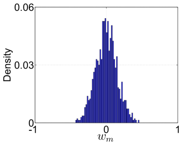
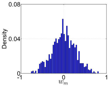
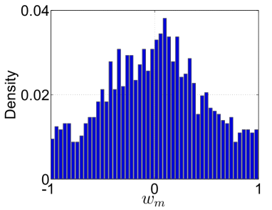
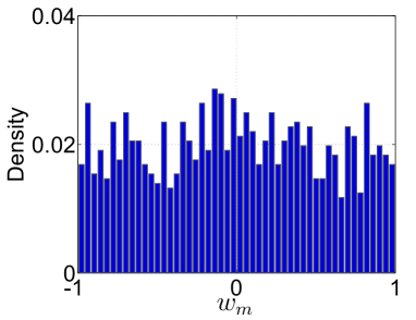
where . In our experiments, we set the sampling interval s such that the required conditions in Theorem 1 are satisfied. Fig. 1 shows the histogram of (i.e., the components in ) under different choices of when the SNR is set to dB. We see that the error induced by the measurement noise becomes significantly larger as increases.
To overcome this difficulty caused by the higher-order difference, in the following, we explore the properties of the first-order difference of modulo samples, and develop algorithms that are robust against noise.
V Robust Compressive Sensing Based Approach
This proposed approach is based on the observation that, although the first-order difference of the modulo samples are not exactly the same as the first-order difference of the original signal samples, these two indeed coincide with a high probability when the sampling rate is sufficiently high. To illustrate this, consider the following example
| (23) |
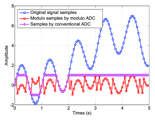
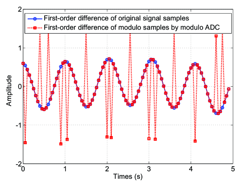
Setting the sampling interval to seconds, Fig. 2(a) shows the undistorted original samples, the samples obtained by a conventional ADC, and the modulo samples obtained by a modulo ADC. The measurable ranges of the conventional ADC and modulo ADC are set to . In Fig. 2(b), the first-order difference of the original samples and that of the modulo samples are plotted. We see that most of the entries are identical. An intuitive explanation of this fact is that when the sampling rate is high, the original signal undergo slow variations between successive samples. As a result, the first-order difference of the original signal samples equals to that of the modulo samples with a high probability.
In fact, those inconsistent samples can be considered as outliers. Thus the LSE problem can be reformulated as a robust sparse signal recovery problem. First, we formulate the first-order difference of modulo samples as
| (24) |
where , , and is an unknown, sparse outlier vector. Note that the above equation comes from the fact that when the sampling rate is sufficiently high, the first-order difference of the modulo samples can be expressed as a sum of the first-order difference of original signal samples and a sparse outlier vector, i.e.
| (25) |
The problem of estimating from (24) is a classic robust sparse signal recovery problem which has been extensively investigated, e.g. [22, 23, 24, 25, 26, 27, 28]. Specifically, a theoretical analysis conducted in [23] shows that under certain conditions, exact recovery of the sparse vector from sparse outlier-corrupted measurements can be guaranteed. In addition to theoretical justifications, many robust compressed sensing algorithms were developed from either optimization-based or Bayesian inference frameworks. Popular algorithms include the outlier-compensation-based approach [25, 26], and outlier identify-and-reject approach [28]. Algorithm 1 summarizes the proposed robust compressive sensing (RCS) based solution for the LSE problem with modulo samples.
Clearly, exact recovery of the sparse signal is feasible when most measurements of are not outliers, in other words, when is sufficiently sparse. Intuitively, given other parameters fixed, the sparsity of the outlier vector is related to the sampling rate: the higher the sampling rate, the sparser the outlier vector. In the following, we provide a quantitative analysis which establishes a mathematical relationship between the sampling rate and the sparsity of the outlier vector obtained via the first-order difference operation.
Remark 2
One issue with the compressive sensing approach is whether the sensing matrix satisfies the restricted isometry property (RIP). While the RIP is generally intractable to verify for generic dictionaries, recent studies showed that the isometry constant can be upper bounded by the mutual coherence of the matrix as follows [29, 30]
| (26) |
Therefore, we can check the RIP of by examining its mutual coherence. Taking and as an example (the same setup as in our simulations), we find that when , the mutual coherence of is consistently less than . Under such a circumstance, we can conclude that
| (27) |
To guarantee , one has , meaning that satisfies the RIP condition when is no greater than .
V-A Theoretical Analysis
The line spectral model in (10) can be re-expressed as
| (28) |
where denotes the argument of the complex parameter , and are, respectively, the real and imaginary parts of which are given as
| (29) | ||||
| (30) |
where . We see that the two sinusoidal mixture functions and share the same frequency components with different phases. To analyze the relationship between the first-order difference of and the first-order difference of its modulo samples, if suffices to examine the first-order difference of either its real component or its imaginary component.
Specifically, consider the following sinusoidal mixture
| (31) |
where , and are, respectively, the phase, frequency and amplitude of the th component. Define , , and . Let and respectively denote the original sample and the modulo sample of , where is the sampling interval. Let denote the first-order difference of the original samples and denote the first-order difference of the modulo samples.
According to (1), the modulo sample of can be written as
| (32) |
The above equation can be re-expressed as
| (33) |
Here is a sum of two terms, where the first term is the quantization output of that is quantized by a step size of , and the second term can be considered as the quantization noise.
Assumption 1
The phase of each component in is a random variable which follows a uniform distribution, i.e.,
| (36) |
Under such an assumption, can be modeled as a uniform random variable when is sufficiently small:
| (37) |
A rigorous justification of the uniform distribution of is discussed in Appendix A.
We are now in a position to present our main result, which is summarized as follows.
Theorem 2
Consider a sinusoidal mixture signal which has a form of (31), where the phase of each sinusoidal component follows a uniform distribution . If the sampling interval satisfies
| (38) |
then the first-order difference of the original samples equals the first-order difference of the modulo samples with probability exceeding
| (39) |
Proof:
See Appendix B. ∎
Theorem 2 indicates that the probability of can be made arbitrarily close to 1 by increasing the sampling rate . Specifically, to make sure that is no less than a pre-specified threshold , i.e., , the sampling interval needs to satisfy
| (40) |
where is defined as
| (41) |
with denoting the effective number of folding times. We see that the sampling condition in (40) has a form similar to the condition in (16), except that they have different scaling factors.
VI Mixed-Integer Linear Programming Based Recovery Approach
VI-A Motivations and Algorithm Development
It is known that the original sample and the modulo sample satisfy the unique decomposition property: , where is an integer. Similarly, it can be readily verified that the first-order difference of the original samples and the first-order difference of the modulo samples are related as , where is an integer. In the previous section, we observed and proved that given a sufficiently high sampling rate, is a sparse vector with only few nonzero entries. Thus the LSE problem can be cast as a robust sparse signal recovery problem. This formulation, however, fails to utilize the information that is an integer.
In fact, considering the property that is an integer, the LSE problem with noise-free can be formulated as a combinatorial problem [34, 35]
| s.t. | ||||
| (42) |
where represents the -dimensional integer space. Such an optimization problem can be transformed into a mixed integer linear program and solved via the branch-and-bound algorithm [36]. This approach, however, is not suitable when the folding number is large as the search space increases exponentially with the folding number.
To reduce the search space, in this section, we take the first-order difference of modulo samples. Specifically, we have
| (43) |
where is an unknown vector with and . We will show that when the sampling rate exceeds a certain threshold, both the real and imaginary components of entries in belong to the set . Thus we can formulate the LSE problem as
| s.t. | ||||
| (44) |
where is a user-defined parameter. For convenience, we write (44) into a real-valued form, i.e.,
| s.t. | ||||
| (45) |
where , , , and
For the th component of , i.e., , we define two auxiliary variables and such that
| (46) | ||||
| (47) |
Therefore we can re-express and as
| (48) | ||||
| (49) |
where and are vectors with and being their th component respectively, and denotes the set of non-negative real numbers. Such a representation leads to
| s.t. | ||||
| (50) |
Unfortunately, (50) is a mixed-integer quadratic optimization problem, which is in general intractable. To deal with this challenge, we replace the quadratic inequality constraint by a linear constraint, resulting in the following optimization problem
| s.t. | ||||
| (51) |
where is a user-defined parameter and denotes the element-wise inequality. The problem (51) is a mixed-integer linear programming that can be solved via the branch-and-bound algorithm (e.g., the off-the-shelf tool intlinprog in Matlab). Once we obtain , , and , we can construct . The mixed-integer linear programming (MILP) based algorithm for the LSE problem with modulo samples is summarized in Algorithm 2.

VI-B Theoretic Analysis
In this subsection, we examine the condition under which the integer is confined to be in the set . We have the following theorem with respect to the sinusoidal mixture signal defined in (31).
Theorem 3
Consider the ensemble of signals that have a form of (31). If the sampling interval satisfies
| (52) |
then we have , where is an integer which belongs to the set .
Proof:
See Appendix D. ∎
Theorem 3 indicates that, when the sampling rate is higher than the threshold in (52), we can guarantee that is confined to be in the set . Similarly, we can rewrite the required sampling interval as
| (53) |
where is given by
| (54) |
in which is the effective folding number. It is clear that is smaller than since , defined before (40), should be greater than in general. Such a relationship between and means that the sampling rate condition (53) is less restrictive than condition (40).
VII Simulation Results
In this section, we provide simulation results to illustrate the performance of the proposed first-order difference-based methods, namely, the RCS-based method and the MILP-based method. The HOD-based method discussed in Section IV is also included as a benchmark to show the effectiveness of the proposed methods. For the RCS-based method, the sparse Bayesian learning method [37] is employed to solve the formulated robust compressed sensing problem.
VII-A Signal Recovery Performance
We consider sinusoidal components with frequencies are , and the number of discretized grid points, , is set to . For each realization, the complex amplitudes of these three sinusoidal components are set to ensure and . The sampling interval required by each method can be accordingly determined:
| (55) | ||||
| (56) | ||||
| (57) |
For the HOD based method, the order of difference has to satisfy the following condition
| (58) |
where denotes the sampling interval for the HOD based method.
In our simulations, the initial phase of each sinusoidal component is randomly selected from . The signal-to-noise ratio (SNR) is defined as . The range parameter is set to throughout our simulations. The normalized mean square error (NMSE) of and the reconstruction SNR (R-SNR) are used as two metrics to evaluate the estimation accuracy of the complex amplitudes and the frequencies. These two metrics are defined respectively as
| NMSE | (59) | |||
| R-SNR | (60) |
where and denote the true parameters and the estimated ones, respectively.
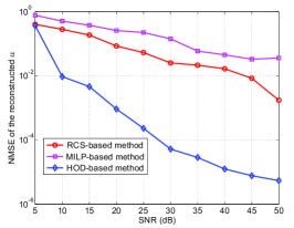
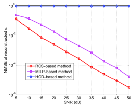
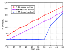
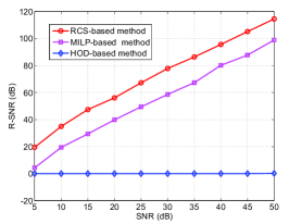
The performance of respective methods along with SNR is plotted in Fig. 3, where three different sampling intervals are employed. We see that the HOD-based method achieves the best performance when s. This is because for the HOD-based method, the required order of difference is when s (cf. (58)), in which case the HOD-based method reduces to a first-order difference method. Nevertheless, when the sampling interval increases to s and s, the required orders of difference for the HOD-based method are and , respectively, in which case the HOD-based method incurs a significant performance degradation. Specifically, when s, the HOD-based method only works for extremely large SNRs (i.e., dB). In contrast, the proposed first-order difference-based methods achieve satisfactory performance across different sampling intervals, ensuring a reliable estimation even under low SNR conditions.
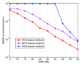
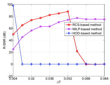
Fig. 4 depicts the NMSEs and the R-SNR of respective methods as the sampling interval varies from s to s with a stepsize of s, where SNR is set to dB. It can be seen that the HOD-based method works well only when the sampling interval is as low as s. This is because the required order of difference is in this case. When the sampling interval increases to s, although it still meets the condition (55), the order of difference required by the HOD-based method is greater than according to (58). Hence the HOD-based method suffers severe performance degradation due to the shrinkage effect on the signal. In contrast, for the proposed first-order difference-based methods, we see that they are able to achieve superior recovery performance even when a smaller sampling rate is employed. In particular, the MILP-based method can provide reliable performance across different values of as long as the condition in (57) is met. The RCS-based method yields a better estimation accuracy than the MILP-based method when . When further increases, the performance of the RCS-based method degrades. Specifically, when s, it can be calculated that the probability of is no less than according to (39). Due to relaxation used in our derivations, this probability is pessimistic. In fact, our experiments suggest that when s, the probability of can reach up to , which implies a majority of elements in are zeros. Hence the sparse outlier assumption required by the RCS-based method is well satisfied, and in this case the RCS-based method outperforms the MILP-based method. When increases to s, our experiments suggest that the probability of drops below . The sparse outlier assumption is barely met in this case. Therefore, when s, the RCS-based method experiences a degraded performance compared to the MILP-based method.
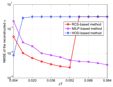
Another interesting observation of Fig. 4 is that, within the region , the performance of the RCS-based and MILP-based methods improves as the sampling interval increases. The is because, when the number of samples is fixed, a larger sampling interval usually results in a less coherent sensing matrix with a more favorable restricted isometry condition, which in turn leads to a better recovery performance. This can be verified by checking the mutual coherence of the sensing matrix , which tends to decrease as the sampling interval increases.
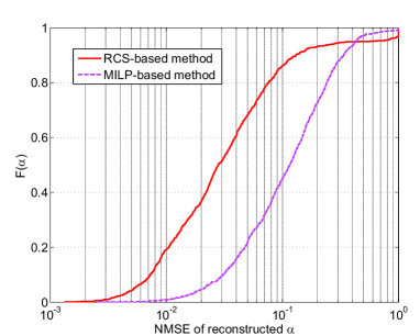
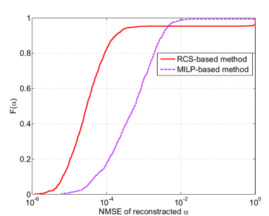
In addition, we consider a scenario where the number of sinusoidal components increases to . For each independent Monte Carlo run, the frequencies of these sinusoidal components are selected from the pre-defined grids, while their amplitudes are randomly selected from a Gaussian distribution . The sampling interval is set to s and the dynamic range of the modulo ADC is set to . We consider two cases, i.e., dB and dB. Results are averaged over independent realizations. Since the sampling interval is fixed while both the frequencies and the amplitudes are randomly selected, the sampling conditions required for the RCS-based method or/and the MILP-based method may not be satisfied. In Fig. 5, we illustrate the empirical PDF of the NMSE of these two cases, and we can see that the MILP-based method has a higher chance to succeed compared with the RCS-based method. This is because the MILP-based method has a more relaxed sampling condition compared with the RCS-based method, as shown in (53) and (40). This result is consistent with the previous conclusion as seen in Fig. 3 and Fig. 4.
VII-B Results with High Dynamic Ranges
The unlimited sensing framework is a potential solution to deal with a difficulty in wireless communications caused by the near-far effect, where due to the limited dynamic range, a weak signal cannot be detected in the presence of a strong background signal. In this experiment, we illustrate the performance of the proposed methods in scenarios with a high dynamic range. To this end, we consider sinusoidal components, and the corresponding parameters are given as
The ratio of the power of the strong signal to the power of the weak signal is dB. To high-fidelity data-acquisition without saturation, a conventional ADC would need a large number of quantization bits. Otherwise the weak signal will be buried beneath the quantization noise level and cannot be effectively detected. Modulo ADCs do not suffer from this issue. Theoretically, modulo ADCs can achieve an unlimited dynamic range by folding the signal back to its range interval. Here we also consider the quantization noise for modulo ADCs. Unlike conventional ADCs, modulo ADCs quantize its modulo samples instead of the original input samples. In our simulations, we set and s.
To evaluate the performance of detecting the weak signal amidst the strong background signal, we use the success rate as a metric: a trial is considered successful if both of the following conditions are met:
-
1.
The support set of the sparse signal is correctly found. In general, most components of the estimated will not exactly equal due to the quantization noise. We set those components to zero if their amplitude is smaller than .
-
2.
The estimation error of each non-zero element, defined as , is no greater than .
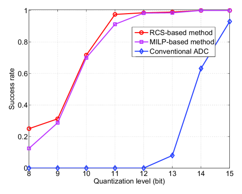
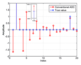
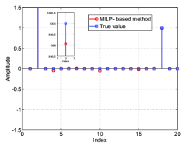
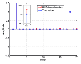
Fig. 6 plots the success rates of respective methods as a function of the number of quantization bits. We see that the success rates of both proposed methods increase when more quantization bits are used. Specifically, a success rate of can be achieved when bits are employed to quantize the modulo samples. In contrast, the conventional ADC needs quantization bits to achieve a decent success rate. In Fig. 7, we plot the estimated for a particular realization when and the number of quantization bits is set to . It can be seen that while the proposed modulo ADC based methods have no difficulty in recovering both the strong and weak signals, the conventional ADC cannot distinguish the weak signal from many false signals it produces.
VIII Conclusions
In this work, we studied the problem of LSE in an unlimited sensing framework, which employs modulo ADCs to nonlinearly map the received signal to modulo samples to avoid clipping or saturation problems. We first introduced a HOD based approach, which is sensitive to noise and lacks satisfactory performance in the presence of noise. To overcome this difficulty, we investigated the properties of the first-order difference of modulo samples, and developed two first-order difference-based methods, namely, the RCS-based and the MILP-based methods. Simulation results show that both methods are robust against noise and achieve a significant performance improvement over the HOD-based method. In practice, due to implementation imperfections of modulo ADCs such as hysteresis effects [18] and impulsive noises [38], the folding numbers might not be integers. How to extend our methods to deal with these nonlinearities is an important topic for future investigation.
Appendix A Discussion On (37)
According to [39], for an input signal to be quantized, if the characteristic function (CF) of the random variable , denoted as , is “bandlimited”, i.e., it satisfies
| (61) |
where is the quantization step size, then the quantization noise follows a uniform distribution. This condition is restrictive, as most frequently encountered signals such as Gaussian signals do not have perfectly bandlimited CFs. Therefore, an approximate condition is widely accepted. Specifically, if is approximately bandlimited for some quantization step size, i.e.,
| (62) |
then the quantization noise can be approximately modeled as a uniform distribution.
In our problem, we assume that the phase of the th component, i.e., , is uniform in the interval . Therefore, the probability density function of is given by [31, 32, 33]
| (66) |
Accordingly, the CF of the random variable is given by [31]
| (67) |
where denotes the Bessel function of the first kind. Note that the CF of the sum of independent random variables is the product of individual CFs associated with these random variables. Therefore, the CF of can be calculated as
| (68) |
Note that the Bessel function when . Hence we have
| (69) |
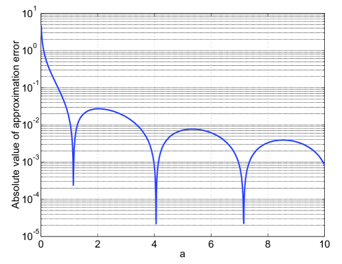
where . In addition, the Bessel function is an even function and looks like a decaying sinusoid that decays proportionally to . Specifically, for , can be approximated as [40]
| (70) |
The absolute value of the approximation error in (70) is shown in Fig. 8, where we can see that, when , the absolute error is less than . In the following, we suppose that (70) holds exactly (i.e., the approximation error is negligible) when .
Setting , has a faster decaying rate than . When , we have
| (71) |
where is directly from (69), and in we employ the approximation in (70). From (71) we know that if
| (72) |
then the following inequality holds
| (73) |
where is a small positive value. Generally, is set sufficiently small such that (specifically, is required to be no greater than ). Therefore, the condition in (72) is equivalent to
| (74) |
Based on the above result, to ensure that the approximately bandlimited condition (62) holds, the following condition should be satisfied
| (75) |
The above condition implies
| (76) |
Considering the fact that and , we have
| (77) |
to ensure (75).
From (77), we know that the operation range of the modulo ADC, i.e., , should be smaller than , such that can be approximately modeled as a uniform distribution. This is equivalent to the condition that the maximum folding number, defined by , should satisfy the following inequality:
| (78) |
If we set and , should be no less than . This condition is usually met considering the fact that the unlimited sensing framework aims to deal with high dynamic range problems.
Appendix B Proof of Theorem 2
By the modulo decomposition property [10], we have
where . Therefore, we have
| (79) |
where . Therefore, can be uniquely represented by a sum of and an unknown constant. In scenarios where this constant equals , is equivalent to . Therefore, we have
| (80) |
By the definition of the modulo operation in (1), we have
| (81) |
which indicates that
| (82) |
Similarly, can be expressed as
| (83) |
Combining (82) and (83) results in
| (84) |
Since is continuous and differentiable on the interval , based on the mean value theorem, there exists a value such that
| (85) |
where is the derivative of . Substituting (85) into (84), we arrive at
| (86) |
where and are, respectively, defined as
By these definitions we have
| (87) |
where is defined as
| (88) |
The derivative of is given by
| (89) |
which leads to the following bound
| (90) |
As in (33), can be expressed as
| (91) |
where can be modeled as a uniform distribution:
| (92) |
In addition, from the quantization theory in [39], is statically independent of . Taking a simple algebraic operation on (91) results in
| (93) |
where also follows a uniform distribution, i.e., . Recalling the definition of , we have
| (94) |
Therefore, can be assumed to follow a uniform distribution over the interval :
| (95) |
For , it can be modeled as a random variable and its distribution is given as (as we have )
| (98) |
where is an arbitrary distribution that satisfies
| (99) |
Furthermore, it is reasonable to assume that and are independent of each other. This is because the quantization noise, , is independent of , and is only related to the derivative of . In this case, the probability density function (PDF) of is given by the convolution of and , i.e.,
| (100) |
Recall that the sampling interval satisfies
| (101) |
Hence we have
| (102) |
and consequently, . Therefore, can be calculated as
| (108) |
where is the cumulative distribution function (CDF) of . The derivation of can be found in Appendix C. The desired probability is then computed as
| (109) |
where , and are respectively calculated by
| (110) | ||||
| (111) | ||||
| (112) |
Therefore, we have
| (113) |
Due to the property of CDF, is non-negative and non-decreasing over the interval . Therefore, the following holds:
| (114) |
Combining (113) and (114), we arrive at our main result
| (115) |
This completes our proof.
Appendix C Derivation of
The PDF of can be expressed as
| (116) |
where in we utilize the definition . Recall that is nonzero only within the interval . Therefore we have if or (i.e., or ).
On the other hand, when , i.e., , we have
| (117) |
Moreover, when and , i.e., , we have
| (118) |
Also, when , i.e., , we have
| (119) |
Summarizing the above results, we arrive at (100).
Appendix D Proof of Theorem 3
From (86), we know that can be expressed by
| (120) |
where . Based on (90), we know that
| (121) |
Recalling (52), we have
| (122) |
which indicates that belongs to the set
| (123) |
On the other hand, we know that
| (124) |
Combining (123) and (124) we obtain that
| (125) |
Therefore belongs to the set , which implies that . This completes the proof.
References
- [1] B. Liao, S.-C. Chan, L. Huang, and C. Guo, “Iterative methods for subspace and DOA estimation in nonuniform noise,” IEEE Transactions on Signal Processing, vol. 64, no. 12, pp. 3008–3020, 2016.
- [2] R. Carriere and R. L. Moses, “High resolution radar target modeling using a modified Prony estimator,” IEEE Transactions on Antennas and Propagation, vol. 40, no. 1, pp. 13–18, 1992.
- [3] J. L. Flanagan, Speech analysis synthesis and perception. Springer Science & Business Media, 2013, vol. 3.
- [4] P. Stoica, R. L. Moses et al., Spectral analysis of signals. Pearson Prentice Hall Upper Saddle River, NJ, 2005, vol. 452.
- [5] J. F. Hauer, C. Demeure, and L. Scharf, “Initial results in Prony analysis of power system response signals,” IEEE Transactions on Power Systems, vol. 5, no. 1, pp. 80–89, 1990.
- [6] M. H. Gruber, “Statistical digital signal processing and modeling,” 1997.
- [7] R. Roy and T. Kailath, “ESPRIT-estimation of signal parameters via rotational invariance techniques,” IEEE Transactions on acoustics, speech, and signal processing, vol. 37, no. 7, pp. 984–995, 1989.
- [8] J. Fang, F. Wang, Y. Shen, H. Li, and R. S. Blum, “Super-resolution compressed sensing for line spectral estimation: An iterative reweighted approach,” IEEE Transactions on Signal Processing, vol. 64, no. 18, pp. 4649–4662, 2016.
- [9] A. Bhandari, F. Krahmer, and R. Raskar, “On unlimited sampling,” in 2017 International Conference on Sampling Theory and Applications (SampTA). IEEE, 2017, pp. 31–35.
- [10] ——, “On unlimited sampling and reconstruction,” IEEE Transactions on Signal Processing, vol. 69, pp. 3827–3839, 2020.
- [11] ——, “Unlimited sampling of sparse signals,” in 2018 IEEE International Conference on Acoustics, Speech and Signal Processing (ICASSP). IEEE, 2018, pp. 4569–4573.
- [12] ——, “Unlimited sampling of sparse sinusoidal mixtures,” in 2018 IEEE International Symposium on Information Theory (ISIT). IEEE, 2018, pp. 336–340.
- [13] H. Wang, X. Zheng, and H. Li, “Kalman filtering with unlimited sensing,” in ICASSP 2024-2024 IEEE International Conference on Acoustics, Speech and Signal Processing (ICASSP). IEEE, 2024, pp. 9826–9830.
- [14] S. Fernández-Menduina, F. Krahmer, G. Leus, and A. Bhandari, “DOA estimation via unlimited sensing,” in 2020 28th European Signal Processing Conference (EUSIPCO). IEEE, 2021, pp. 1866–1870.
- [15] S. Fernández-Menduiña, F. Krahmer, G. Leus, and A. Bhandari, “Computational array signal processing via modulo non-linearities,” IEEE Transactions on Signal Processing, vol. 70, pp. 2168–2179, 2022.
- [16] A. Bhandari, F. Krahmer, and T. Poskitt, “Unlimited sampling from theory to practice: Fourier-Prony recovery and prototype ADC,” IEEE Transactions on Signal Processing, vol. 70, pp. 1131–1141, 2021.
- [17] D. Florescu, F. Krahmer, and A. Bhandari, “Unlimited sampling with hysteresis,” in 2021 55th Asilomar Conference on Signals, Systems, and Computers. IEEE, 2021, pp. 831–835.
- [18] ——, “The surprising benefits of hysteresis in unlimited sampling: Theory, algorithms and experiments,” IEEE Transactions on Signal Processing, vol. 70, pp. 616–630, 2022.
- [19] ——, “Event-driven modulo sampling,” in ICASSP 2021-2021 IEEE International Conference on Acoustics, Speech and Signal Processing (ICASSP). IEEE, 2021, pp. 5435–5439.
- [20] A. Bhandari, “Back in the US-SR: Unlimited sampling and sparse super-resolution with its hardware validation,” IEEE Signal Processing Letters, vol. 29, pp. 1047–1051, 2022.
- [21] J. A. Tropp and A. C. Gilbert, “Signal recovery from random measurements via orthogonal matching pursuit,” IEEE Transactions on Information Theory, vol. 53, no. 12, pp. 4655–4666, 2007.
- [22] J. Wright, A. Y. Yang, A. Ganesh, S. S. Sastry, and Y. Ma, “Robust face recognition via sparse representation,” IEEE Transactions on Pattern Analysis and Machine Intelligence, vol. 31, no. 2, pp. 210–227, 2008.
- [23] N. H. Nguyen and T. D. Tran, “Robust lasso with missing and grossly corrupted observations,” IEEE Transactions on Information Theory, vol. 59, no. 4, pp. 2036–2058, 2012.
- [24] ——, “Exact recoverability from dense corrupted observations via -minimization,” IEEE Transactions on Information Theory, vol. 59, no. 4, pp. 2017–2035, 2013.
- [25] R. E. Carrillo and K. E. Barner, “Lorentzian iterative hard thresholding: Robust compressed sensing with prior information,” IEEE Transactions on Signal Processing, vol. 61, no. 19, pp. 4822–4833, 2013.
- [26] E. Ollila, H.-J. Kim, and V. Koivunen, “Robust iterative hard thresholding for compressed sensing,” in 2014 6th International Symposium on Communications, Control and Signal Processing (ISCCSP). IEEE, 2014, pp. 226–229.
- [27] J. T. Parker, P. Schniter, and V. Cevher, “Bilinear generalized approximate message passing—part I: Derivation,” IEEE Transactions on Signal Processing, vol. 62, no. 22, pp. 5839–5853, 2014.
- [28] Q. Wan, H. Duan, J. Fang, H. Li, and Z. Xing, “Robust Bayesian compressed sensing with outliers,” Signal Processing, vol. 140, pp. 104–109, 2017.
- [29] M. Elad, “Optimized projections for compressed sensing,” IEEE Transactions on Signal Processing, vol. 55, no. 12, pp. 5695–5702, 2007.
- [30] M. Yang and F. de Hoog, “New coherence and rip analysis for weak orthogonal matching pursuit,” in 2014 IEEE Workshop on Statistical Signal Processing (SSP). IEEE, 2014, pp. 376–379.
- [31] R. Barakat, “First-order statistics of combined random sinusoidal waves with applications to laser speckle patterns,” Optica Acta, vol. 21, no. 11, pp. 903–921, 1974.
- [32] R. Barakat and J. Cole III, “Statistical properties of random sinusoidal waves in additive Gaussian noise,” Journal of Sound and Vibration, vol. 62, no. 3, pp. 365–377, 1979.
- [33] A. Papoulis and S. Unnikrishna Pillai, Probability, Random variables and Stochastic Processes (4th edition). McGraw-Hill: New York, NY, USA, 2002.
- [34] D. Prasanna, C. Sriram, and C. R. Murthy, “On the identifiability of sparse vectors from modulo compressed sensing measurements,” IEEE Signal Processing Letters, vol. 28, pp. 131–134, 2020.
- [35] O. Musa, P. Jung, and N. Goertz, “Generalized approximate message passing for unlimited sampling of sparse signals,” in 2018 IEEE Global Conference on Signal and Information Processing (GlobalSIP). IEEE, 2018, pp. 336–340.
- [36] J. Clausen, “Branch and bound algorithms-principles and examples,” Department of Computer Science, University of Copenhagen, pp. 1–30, 1999.
- [37] D. P. Wipf and B. D. Rao, “Sparse Bayesian learning for basis selection,” IEEE Transactions on Signal Processing, vol. 52, no. 8, pp. 2153–2164, 2004.
- [38] A. Bhandari, “Unlimited sampling with sparse outliers: Experiments with impulsive and jump or reset noise,” in ICASSP 2022-2022 IEEE International Conference on Acoustics, Speech and Signal Processing (ICASSP). Singapore, 2022, pp. 5403–5407.
- [39] B. Widrow, I. Kollar, and M.-C. Liu, “Statistical theory of quantization,” IEEE Transactions on Instrumentation and Measurement, vol. 45, no. 2, pp. 353–361, 1996.
- [40] M. Abramowitz, I. A. Stegun et al., Handbook of mathematical functions. Dover New York, 1964, vol. 55.