Generalized flow-composed symplectic methods for post-Newtonian Hamiltonian systems

Abstract

Due to the nonseparability of the post-Newtonian (PN) Hamiltonian systems of compact objects, the symplectic methods that admit the linear error growth and the near preservation of first integrals are always implicit as explicit symplectic methods have not been currently found for general nonseparable Hamiltonian systems. Since the PN Hamiltonian has a particular formulation that includes a dominant Newtonian part and a perturbation PN part, we present the generalized flow-composed Runge–Kutta (GFCRK) method with a free parameter $\lambda$ to PN Hamiltonian systems. It is shown that the GFCRK method is symplectic once the underlying RK method is symplectic, and it is symmetric once the underlying RK method is symmetric under the setting $\lambda=1/2$. Numerical experiments with the 2PN Hamiltonian of spinning compact binaries demonstrate the higher accuracy and efficiency of the symplectic GFCRK method than the underlying symplectic RK. Meanwhile, the numerical results also support higher efficiency of the symplectic GFCRK method than the semi-explicit mixed symplectic method of the same order.

1 Introduction

Post-Newtonian (PN) Hamiltonian approach has been verified to be a good weak-filed approximation to general relativity. It is usually used to model the system of compact objects in the early stage of the inspiral [1]. Except for some qualitative results on the dynamics of PN Hamiltonian systems [2, 3, 4], the numerical simulation involving the design and implementation of numerical integration methods has been necessary for PN Hamiltonian systems.

Numerous numerical methods have been developed to solve the PN Hamiltonian system numerically. The generic designing methods mainly include the single-step method such as the classical Runge–Kutta (RK) method and linear multistep methods, and high-order methods are often employed for short-term orbit prediction [5]. However, for long-term dynamical investigation, these generic designing methods always failed to obtain reliable numerical solutions due to the extremely enlarged truncation errors, which are caused by the at least quadratic growth of global errors with respect to the integration time [6].

The development of symplectic methods [7, 8] takes a great advantage to the numerical solving of Hamiltonian systems, since symplectic methods admit a linear error growth for near-integrable Hamiltonian systems and could nearly preserve the first integrals of the Hamiltonian. Up to now, symplectic methods have been well developed for Hamiltonian problems. Except for the generic symplectic methods for general Hamiltonian systems, such as the symplectic Runge–Kutta [9] method and the generating function method [8], typical explicit symplectic methods for Newtonian N-body problems include the standard $T+V$ splitting methods [10, 11], the $H_{0}+\varepsilon H_{1}$ splitting methods [12], the force gradient methods [13, 14, 15], and the pseudo-high-order methods [16, 17, 18, 19] by taking account of the separability of the Hamiltonian.

However, for the post-Newtonian N-body problems, the Hamiltonian is always nonseparable even though sometimes it may be integrable in the case where the spin-spin effect is not included in the Hamiltonian [3]. Once the PN Hamiltonian is nonseparable, there is no explicit symplectic method, and then implicit symplectic methods are necessary for the accurate long-term investigation. Although the fully implicit symplectic Runge–Kutta or partitioned Runge–Kutta methods [7] are available, their computational efficiency are low due to the iteration used during the implementation. Instead, Lubich et al. [20], Zhong et al. [21], and Mei et al. [22] proposed the mixed symplectic method that exact solves the integrable Newtonian part and numerically solves the perturbed PN part by symplectic implicit midpoint method. It is shown that the mixed symplectic method is more efficient than the same-order fully implicit symplectic RK-type method.

Because of the use of iterations in the implementation, the mixed symplectic method is essentially implicit. Recently, Mei & Huang [23] improved the mixed symplectic method to the explicit near-symplectic method by replacing the implicit midpoint method with classical explicit RK methods to solve the PN perturbation part. Although the short-term behavior of the improved explicit near-symplectic method is nearly the same as the underlying mixed symplectic method on the presence of the small perturbation parameter, the time interval on which the linear error growth holds will be much shorter than the original mixed symplectic method.

We also note that although the explicit [24, 25, 26] or the implicit [27] extended phase space methods perform well in the energy error in the numerical simulation of PN Hamiltonian systems, the symplecticitiy of these explicit methods in the original phase space and thus the most important property of linear error growth is indefinite. It should be emphasized that the linear error growth of the explicit extended phase space method made by Tao [25] just holds under the assumption that the extended Hamiltonian system is near-integrable or integrable. However, as indicated by the simple example of [25], a completely integrable Hamiltonian could lead to a nonintegrable extended Hamiltonian, we thus consider the near-integrability of extended Hamiltonian is hardly satisfied.

Besides the above-mentioned symplectic methods, Antoñana, Makazaga & Murua [28] proposed a new class of symplectic methods for the Newtonian N-Body problem. This new symplectic method is referred to as symplectic flow-composed Runge–Kutta (FCRK)method, where the phase flow of the Kepler two-body problem is employed to transform the original system into a flow-composed Hamiltonian system. Since the Kepler flow of the two-body problem dominates the evolution of the system, the FCRK method shows much higher accuracy in the numerical simulation of the N-body problem of our Solar System. Motivated by the FCRK method, in this paper, we aim to adapt the symplectic FCRK method to the PN Hamiltonian system. We find that the FCRK method could be generalized with a free parameter $\lambda$, where $\lambda=1/2$ just reduces to the original FCRK method proposed in [28]. A preliminary analysis shows that the setting $\lambda=0$ and $\lambda=1$ could slightly decrease the computation amount. Moreover, the complete freedom of $\lambda$ enables us to minimize the truncation error in principle or to preserve the energy or other first integrals.

This paper is organized as follows. In Section 2, we formulate the second-order PN Hamiltonian of spinning compact binaries in the canonically conjugate variables. In Section 3, we derive the GFCRK method and present a detailed discussion on the property and its relation with the mixed symplectic method. Numerical experiments are presented in Section 4 by showing the global errors, the energy errors, and the consumed CPU time to verify the convergence order and the high efficiency of the GFCRK method. We draw our conclusions in the last section.

2 Post-Newtonian Hamiltonian formulation

Since the PN terms are in a smaller magnitude than the Newtonian term of the N-body problem, the PN Hamiltonian of the N-body problem is in a uniform formulation with the dominant Newtonian part and a PN perturbation part [29, 30, 31, 32, 33, 34, 35, 36, 37]. Without loss of generality, in this paper we only take the conservative PN Hamiltonian of spinning compact binaries as an example. The application of the generalized FCRK method to other PN Hamiltonian systems could be extended similarly.

The PN Hamiltonian of spinning compact binaries considered in this paper is accurate up to 2PN order. Once formulated in the Arnowitt-Deser-Misner (ADM) coordinates and in the center-of-mass frame, the Hamiltonian reads

$$H(\bm{Q},\bm{P},\bm{S}_{1},\bm{S}_{2})=H_{N}+\frac{1}{c^{2}}H_{1PN}+\frac{1}{c^{4}}H_{2PN}+\frac{1}{c^{3}}H_{1.5PN}^{SO}+\frac{1}{c^{4}}H_{2PN}^{SS}.$$ (2.1)

where $\bm{P}$ is the momenta of body 1 relative to the center, $\bm{Q}$ is the position coordinates of body 1 relative to body 2, $\bm{S}_{i}~{}(i=1,2)$ are the spins of the two compact bodies, $H_{N}$, $H_{1PN}$, and $H_{2PN}$ are respectively the Newtonian term, the 1PN-, and 2PN-order orbital contributions, $H_{1.5PN}^{SO}$ is the spin-orbit couplings of 1.5PN order, and $H_{SS}$ is the spin-spin couplings and accurate up to 2PN order.

Let $\bm{N}=\bm{Q}/r$ be the unit vector, $r=|\bm{Q}|=\sqrt{q_{1}^{2}+q_{2}^{2}+q_{3}^{2}}$, $m_{1}$ and $m_{2}~{}(m_{1}\leq m_{2})$ be mass of the two compact bodies, $M=m_{1}+m_{2}$ be the total mass, $\beta=m_{1}/m_{2}$ be the mass ratio, and $\eta=\beta/(1+\beta)^{2}$. The orbital terms could be expressed as follows [38]

$$H_{N} =\frac{\bm{P}^{2}}{2}-\frac{1}{r}$$

$$H_{1PN} =\frac{1}{8}(3\eta-1)\bm{P}^{4}-\frac{1}{2}\big{[}(3+\eta)\bm{P}^{2}+\eta(\bm{N}\cdot\bm{P})^{2}\big{]}\frac{1}{r}+\frac{1}{2r^{2}},$$

$$H_{2PN} =\frac{1}{16}(1-5\eta+5\eta^{2})\bm{P}^{6}+\frac{1}{8}\big{[}(5-20\eta-3\eta^{2})\bm{P}^{4}-2\eta^{2}{(\bm{N}\cdot\bm{P})^{2}}\bm{P}^{2}$$

$$\quad-3\eta^{2}{(\bm{N}\cdot\bm{P})^{4}}\big{]}\frac{1}{r}+\frac{1}{2}\big{[}(5+8\eta)\bm{P}^{2}+3\eta(\bm{N}\cdot\bm{P})^{2}\big{]}\frac{1}{r^{2}}-\frac{1}{4}(1+3\eta)\frac{1}{r^{3}}.$$

Moreover, the spin-orbit [39] and spin-spin [38] terms are respectively:

$$H_{1.5PN}^{SO} =\frac{1}{r^{3}}\big{(}2\bm{S}+\frac{3}{2}\bm{S}^{*}\big{)}\cdot\bm{L},$$

$$H_{2PN}^{SS} =\frac{1}{2r^{3}}\big{[}3(\bm{S}_{0}\cdot\bm{N})^{2}-\bm{S}_{0}^{2}\big{]},$$

where $\bm{S}=\bm{S}_{1}+\bm{S}_{2}$, $\bm{S}^{*}=\frac{1}{\beta}\bm{S}_{1}+\beta\bm{S}_{2}$, $\bm{S}_{0}=\bm{S}+\bm{S}^{*}$, and $\bm{L}$ is the orbital angular momentum vector $\bm{L}=\bm{Q}\times\bm{P}$.

For the gravitational constant $G$ and the total mass $M$, we employ the convenient geometric unit $G=M=1$. As explained in [40, 33, 34, 41], the rescaled speed of light $c$ should be readjusted to coincide with specific physical phenomena under the setting $G=M=1$. A smaller value of $c$ for (2.1) usually indicates a stronger PN effect. The details on the discussion of $c$ can be found in [34, 41].

Because the evolution equations of (2.1) read

$$\frac{\mathrm{d}\bm{Q}}{\mathrm{d}t}=\frac{\partial{H}}{\partial\bm{P}},\qquad\frac{\mathrm{d}\bm{P}}{\mathrm{d}t}=-\frac{\partial{H}}{\partial\bm{Q}},\qquad\frac{\mathrm{d}\bm{S}_{i}}{\mathrm{d}t}=\frac{\partial{H}}{\partial\bm{S}_{i}}\times\bm{S}_{i},~{}~{}i=1,2,$$ (2.2)

the spin variables $\bm{S}_{i}$ are not canonically conjugate to each other. On noting the conservation of the spin magnitudes $|\bm{S}_{i}|$ during the evolution of the system, Wu & Xie [42] introduced the canonical conjugate spin variables $\bm{\theta}=(\theta_{1},\theta_{2})$ and $\bm{\xi}=(\xi_{1},\xi_{2})$:

$$\bm{S}_{i}=\left(\begin{aligned} &\rho_{i}\cos(\theta_{i})\\ &\rho_{i}\sin(\theta_{i})\\ &\quad\xi_{i}\end{aligned}\right),\quad i=1,2,$$ (2.3)

where $\rho_{i}^{2}+\xi_{i}^{2}=\Lambda_{i}^{2}$, $\rho_{i}>0$, and $\Lambda_{i}=|\bm{S}_{i}|$ for $i=1,2$. Usually, the spin magnitudes are expressed as $\Lambda_{i}=\chi_{i}m_{i}^{2}/M^{2}$ with $\chi_{i}\in[0,1]$. Because of the conservation of $\Lambda_{i}$, the usage of the new canonical conjugate spin variables reduces the 12-dimensional noncanonical Hamiltonian system $H(\bm{Q},\bm{P},\bm{S}_{1},\bm{S}_{2})$ to a 10-dimensional canonical Hamiltonian system $H(\bm{Q},\bm{P},\bm{\theta},\bm{\xi})$, where the canonical equations follow that

$$\frac{\mathrm{d}\bm{Q}}{\mathrm{d}t}=\frac{\partial{H}}{\partial\bm{P}},\qquad\frac{\mathrm{d}\bm{P}}{\mathrm{d}t}=-\frac{\partial{H}}{\partial\bm{Q}},\qquad\frac{\mathrm{d}\bm{\theta}}{\mathrm{d}t}=\frac{\partial{H}}{\partial\bm{\xi}},\qquad\frac{\mathrm{d}\bm{\xi}}{\mathrm{d}t}=-\frac{\partial{H}}{\partial\bm{\theta}}.$$ (2.4)

3 New symplectic method with composed flows

3.1 Generalized flow-composed method

To describe the numerical method, we let $\bm{z}=(\bm{P},\bm{\xi},\bm{Q},\bm{\theta})$, $I_{5}$ be the $5\times 5$ identity matrix, and $J=\left(\begin{array}[]{cc}O&I_{5}\\ -I_{5}&O\\ \end{array}\right)$ be the canonical skew-symmetric matrix. Then, the canonical equations corresponding to $H(\bm{z}):=H(\bm{Q},\bm{P},\bm{\theta},\bm{\xi})$ could be formally written as

$$\frac{\mathrm{d}\bm{z}}{\mathrm{d}t}=J^{-1}\nabla H(\bm{z}).$$ (3.1)

Since the rescaled parameter $c$ is usually in a magnitude smaller than 1, we spit the Hamiltonian (2.1) into two parts as follows:

$$H(\bm{z})=H_{N}+\varepsilon H_{PN},$$ (3.2)

where $\varepsilon=\frac{1}{c^{2}}<1$ and $H_{PN}=H_{1PN}+\varepsilon H_{2PN}+\sqrt{\varepsilon}H_{1.5PN}^{SO}+\varepsilon H_{2PN}^{SS}$. Using the notations $f=J^{-1}\nabla H_{N}$ and $g=J^{-1}\nabla H_{PN}$, we rewrite the equation (3.1) as follows:

$$\frac{\mathrm{d}\bm{z}}{\mathrm{d}t}=f(\bm{z})+\varepsilon g(\bm{z}).$$ (3.3)

Because $H_{N}$ is just the Hamiltonian of the Newtonian two-body problem, it is completely integrable and could be exactly solved in principle. Therefore, we assume that there exists the phase flow $\phi_{t}:\bm{z}_{0}\mapsto\bm{z}(t)$ such that $\bm{z}(t)$ is the solution of the initial-value problem

$$\frac{\mathrm{d}\bm{z}}{\mathrm{d}t}=f(\bm{z}),\quad\bm{z}(0)=\bm{z}_{0},$$

corresponding to the Hamiltonian $H_{N}$. Let $\tau$ be a given constant and consider the change of variables:

$$\bm{z}(t)=\phi_{t-\tau}(\bm{w}(t)),$$ (3.4)

the canonical equation (3.3) is transformed into

$$\frac{\mathrm{d}\bm{w}}{\mathrm{d}t}=\varepsilon\Big{(}\frac{\partial\phi_{t-\tau}(\bm{w})}{\partial\bm{w}}\Big{)}^{-1}g\big{(}\phi_{t-\tau}(\bm{w})\big{)},$$ (3.5)

in the new variables $\bm{w}$.

Since $\phi_{t}$ is the phase flow of the Hamiltonian $H_{N}$, the Joacobian $\frac{\partial\phi_{t-\tau}(\bm{w})}{\partial\bm{w}}$ is symplectic and nonsingular, i.e.,

$$\Big{(}\frac{\partial\phi_{t-\tau}(\bm{w})}{\partial\bm{w}}\Big{)}^{\intercal}J\Big{(}\frac{\partial\phi_{t-\tau}(\bm{w})}{\partial\bm{w}}\Big{)}=J,$$

which means

$$\Big{(}\frac{\partial\phi_{t-\tau}(\bm{w})}{\partial\bm{w}}\Big{)}^{-1}J^{-1}=J^{-1}\Big{(}\frac{\partial\phi_{t-\tau}(\bm{w})}{\partial\bm{w}}\Big{)}^{\intercal}.$$

On noting $g=J^{-1}\nabla H_{PN}$, we thus derive from (3.5) that

$$\frac{\mathrm{d}\bm{w}}{\mathrm{d}t}=\varepsilon J^{-1}\Big{(}\frac{\partial\phi_{t-\tau}(\bm{w})}{\partial\bm{w}}\Big{)}^{\intercal}\nabla H_{PN}\big{(}\phi_{t-\tau}(\bm{w})\big{)},$$ (3.6)

which is just the canonical equation of the Hamiltonian

$$\mathcal{H}(\bm{w})=\varepsilon H_{PN}\big{(}\phi_{t-\tau}(\bm{w})\big{)}.$$ (3.7)

Now, we consider the constant stepsize numerical method. Suppose that $h$ is the stepsize, the Hamiltonian is numerically integrated on the interval $[0,T_{end}]$. Suppose that $\tau=t_{0}+\lambda h$ where $\lambda$ is a constant. Let $t=t_{0}+\zeta h$ and $\widetilde{\bm{w}}(\zeta)=\bm{w}(t_{0}+\zeta h)$, we restrict the equation (3.6) in the typical interval $t\in[t_{0},t_{0}+h]$ or equivalently $\zeta\in[0,1]$ as an initial-value problem:

$$\frac{\mathrm{d}\widetilde{\bm{w}}}{\mathrm{d}\zeta}=h\varepsilon J^{-1}\Big{(}\frac{\partial\phi_{\zeta h-\lambda h}(\widetilde{\bm{w}})}{\partial\widetilde{\bm{w}}}\Big{)}^{\intercal}\nabla H_{PN}\big{(}\phi_{\zeta h-\lambda h}(\widetilde{\bm{w}})\big{)},$$ (3.8)

with the initial condition

$$\widetilde{\bm{w}}(0)=\bm{w}(t_{0})=\phi_{\lambda h}(\bm{z}(t_{0})).$$ (3.9)

Then, according to (3.4) the solution $\widetilde{\bm{w}}(\zeta)$ of (3.8) satisfies

$$\widetilde{\bm{w}}(\zeta)=\bm{w}(t_{0}+\zeta h)=\phi_{(\lambda-\zeta)h}(\bm{z}(t_{0}+\zeta h)).$$ (3.10)

Let $t_{0}=nh$, $\bm{Z}_{n}\approx\bm{z}(nh)$, $\bm{W}_{n}\approx\bm{w}(nh)$ be the numerical solutions, and

$$G(\zeta,\widetilde{\bm{w}},\lambda,h)=J^{-1}\Big{(}\frac{\partial\phi_{\zeta h-\lambda h}(\widetilde{\bm{w}})}{\partial\widetilde{\bm{w}}}\Big{)}^{\intercal}\nabla H_{PN}\big{(}\phi_{\zeta h-\lambda h}(\widetilde{\bm{w}})\big{)},$$ (3.11)

for $n=0,1,\cdots,N-1$ with $N=T_{end}/h$. According to (3.9) and (3.10), once apply an $s$-stage Runge–Kutta (RK) method with the coefficients $(a_{ij},b_{i},c_{i})_{i,j=1}^{s}$ to the system (3.8) with the initial condition $\widetilde{\bm{w}}(0)=\bm{W}_{n}=\phi_{\lambda h}(\bm{Z}_{n})\approx\bm{w}(nh)$, we yield the numerical scheme as follows:

$$\left\{\begin{aligned} &\bm{W}_{n}=\phi_{\lambda h}(\bm{Z}_{n}),\\ &\bm{G}_{i}=\varepsilon G\big{(}c_{i},\bm{W}_{n}+h\sum_{j=1}^{s}a_{ij}\bm{G}_{j},\lambda,h\big{)},~{}~{}i=1,\cdots,s,\\ &\bm{W}_{n+1}=\bm{W}_{n}+h\sum_{i=1}^{s}b_{i}\bm{G}_{i},\\ &\bm{Z}_{n+1}=\phi_{(1-\lambda)h}(\bm{W}_{n+1}),\end{aligned}\right.$$ (3.12)

which is called generalized flow-composed RK (GFCRK) method in this paper. It is noted that the parameter $\lambda$ is free and usually takes values on the interval $[0,1]$. Once $\lambda=1/2$, the GFCRK method (3.12) reduces to the standard flow-composed RK proposed in [28].

It is observed from the formula of $G(\zeta,\widetilde{\bm{w}},\lambda,h)$ that the evaluation of the function $G$ involves the Jacobian of the phase flow $\phi_{t}(\widetilde{\bm{w}})$. Since we cannot get the explicit expression of $\phi_{t}(\widetilde{\bm{w}})$, the Jacobian is also not explicitly obtained. As recommended by [28], one can use the automatic differentiation technique to compute all the partial derivatives. Moreover, dimension $36$ of the output is larger than dimension $6$ of the input for the automatic differentiation, we consider the forward mode to be more favorable than the reverse mode for the automatic differentiation. In fact, the phase flow $\phi_{t}(\widetilde{\bm{w}})$ of the Newtonian two-body problem contains only an iteration procedure to solve the Kepler equation, its Jacobian could be directly expressed in an easy manner instead of using automatic differentiation.

3.2 Property of GFRCK methods

The properties of the GFRCK method (3.12) certainly depend on the free parameter $\lambda$ and the underlying RK method. We first consider the time-symmetry of the GFCRK method. Suppose that the underlying RK method is symmetric, i.e., the coefficients $(a_{ij},b_{i},c_{i})_{i,j=1}^{s}$ satisfy the conditions [9, 7]

$$c_{s+1-j}=1-c_{j},\quad b_{s+1-j}=b_{j},\quad j=1,\cdots,s,$$

$$a_{ij}+a_{s+1-i,s+1-j}=b_{j},\quad i,j=1,\cdots,s,$$

exchanging $n+1\leftrightarrow n$ and $h\leftrightarrow-h$ yields that the GFCRK method (3.12) is symmetric only if $\lambda=1-\lambda$, i.e., $\lambda=1/2$. Once $\lambda\neq 1/2$, the GFCRK method (3.12) is not symmetric even if the RK method is symmetric under our consideration that $\phi_{t}$ is the phase flow of the Newtonian two-body problem.

Now, we consider the symplecticity of the GFCRK method (3.12). If denote the RK method with the stepsize $h$ by $\Phi_{h}$, then the numerical scheme (3.12) is abstractly expressed by

$$\bm{Z}_{n+1}=\Psi_{h}\big{(}\bm{Z}_{n}\big{)}.$$

where $\Psi_{h}=\phi_{(1-\lambda)h}\circ\Phi_{h}\circ\phi_{\lambda h}$. Since $\phi_{(1-\lambda)h}$ and $\phi_{\lambda h}$ are phase flows of the Hamiltonian $H_{N}$ with different stepsizes, they are both symplectic mappings. This means that the symplecticity of the numerical discrete flow $\Psi_{h}$ remains the same as that of $\Phi_{h}$ on noting the fact that the composition of symplectic mappings is still symplectic. That is, once the RK method is symplectic, i.e., the coefficients $(a_{ij},b_{i},c_{i})_{i,j=1}^{s}$ satisfy the conditions [7]

$$b_{i}a_{ij}+b_{j}a_{ji}=b_{i}b_{j},\quad i,j=1,\cdots,s,$$

the numerical discrete flow $\Psi_{h}$ and thus the GFCRK method (3.12) is symplectic.

Moreover, it is also known that the GFCRK method (3.12) is nonsymplectic provided the RK method is nonsymplectic. A typical example of symplectic RK methods is the second-order implicit midpoint method. Higher-order symplectic RK methods mainly include the Gauss–Legendre collocation method. Here, we present the Butcher tabular of the fourth-order Gauss–Legendre collocation method IRK4 [5, 7] as an example:

$$\begin{array}[]{ccc}\begin{tabular}[]{ c|cc}$c_{1}$&$a_{11}$&$a_{12}$\\ $c_{2}$&$a_{21}$&$a_{22}$\\ \hline\cr&$\raisebox{-2.15277pt}[0.5pt]{$b_{1}$}$&$\raisebox{-2.15277pt}[0.5pt]{$b_{2}$}$\end{tabular}&=&\begin{tabular}[]{ c|cc}$\frac{1}{2}-\frac{\sqrt{3}}{6}$&$\frac{1}{4}$&$\frac{1}{4}-\frac{\sqrt{3}}{6}$\\ $\frac{1}{2}+\frac{\sqrt{3}}{6}$&$\frac{1}{4}+\frac{\sqrt{3}}{6}$&$\frac{1}{4}$\\ \hline\cr&\raisebox{-2.15277pt}[0.5pt]{$\frac{1}{2}$}&\raisebox{-2.15277pt}[0.5pt]{$\frac{1}{2}$}\end{tabular}\end{array}\,.$$

More details on symplectic RK methods can be found in [7].

We next consider the convergence order of the GFCRK method (3.12). Suppose that the underlying RK method is of order $\mu\in\mathbb{N}^{+}$. Under the assumption $\widetilde{\bm{w}}(0)=\bm{W}_{n}=\bm{w}(nh)=\phi_{\lambda h}(\bm{z}(nh))$, we use $\widetilde{\bm{W}}_{n+1}$ and $\widetilde{\bm{Z}}_{n+1}$ to denote the numerical solutions obtained by applying the RK method to (3.8). Due to the appearance of the small parameter $\varepsilon$ in the equation (3.8), it will appear in the local truncation error of $\widetilde{\bm{W}}_{n+1}$ as well. We further note that since the function $G(\zeta,\widetilde{\bm{w}},\lambda,h)$ defined in (3.11) essentially involves the Kepler phase flow $\phi_{t}$, the power of $\varepsilon$ contained in the derivatives of any order of $G(\zeta,\widetilde{\bm{w}},\lambda,h)$ with respect to $\zeta$ is just one. This gives the local truncation error of $\mathcal{O}(\varepsilon h^{\mu+1})$ instead of $\mathcal{O}(\varepsilon^{\mu+1}h^{\mu+1})$ for the numerical solutions $\widetilde{\bm{W}}_{n+1}$, i.e.,

$$\widetilde{\bm{W}}_{n+1}-\bm{w}((n+1)h)=\mathcal{O}(\varepsilon h^{\mu+1}),$$ (3.13)

Because the Hamiltonian $H_{N}$ is completely integrable, the continuous dependency of the phase flow $\phi_{t}$ along with (3.13) leads to that the local error of $\widetilde{\bm{Z}}_{n+1}$ also satisfies

$$\widetilde{\bm{Z}}_{n+1}-\bm{z}((n+1)h)=\mathcal{O}(\varepsilon h^{\mu+1}),$$

which means the global error of the GFCRK method satisfies

$$\bm{Z}_{n}-\bm{z}(nh)=\mathcal{O}(\varepsilon h^{\mu}),$$ (3.14)

for all $n=1,2,\cdots,N$. However, the direct application of the RK method to the canonical equation (3.1) could only yield the following local error estimation

$$\widetilde{\bm{Z}}_{n+1}-\bm{z}((n+1)h)=\mathcal{O}(h^{\mu+1}),$$

which gives the following global error estimation

$$\bm{Z}_{n}-\bm{z}(nh)=\mathcal{O}(h^{\mu}),$$ (3.15)

for all $n=1,2,\cdots,N$. That is, the global error of the GFCRK method will be smaller than that of the underlying RK method with a factor of $\varepsilon<1$ when applied to numerically integrate the post-Newtonian Hamiltonian (2.1).

Once the GFCRK method and its underlying RK method are both symplectic, they are implicit as well. As recommended in [7], we use the fixed-point iteration to find the numerical solutions of $\bm{G}_{i}$ for $i=1,\cdots,s$. In this case, the iteration function of the GFCRK method becomes

$$\mathcal{F}(\bm{G}_{1},\cdots,\bm{G}_{s})=\varepsilon G(\bm{G}_{1},\cdots,\bm{G}_{s}).$$ (3.16)

However, the iteration function of the RK method directly applied to (3.3) will be

$$\mathcal{U}(\bm{G}_{1},\cdots,\bm{G}_{s})=f(\bm{G}_{1},\cdots,\bm{G}_{s})+\varepsilon g(\bm{G}_{1},\cdots,\bm{G}_{s}).$$ (3.17)

The comparison between (3.16) and (3.17) indicates a faster convergence of the GFCRK method than the RK method provided $\varepsilon<1$. This point will also be illustrated by the numerical result in the next section.

For the special case where $H_{N}$ is replaced by a quadratic Hamiltonian and thus $f(\bm{z})$ is linear as a function of $\bm{z}$, the GFCRK method (3.12) will reduce to the Lawson’s generalized RK method, i.e., a class of exponential RK (ERK) methods. In particular, the reduced ERK methods will be the same regardless of the value of $\lambda$. In this case, the time-symmetry and the symplecticity of the ERK method will be the same as the underlying RK method. More details such as the issue of the convergence of the fixed-point iteration for symplectic ERK methods can be found in [43, 44, 45].

We finally consider the dependence of the performance of GFCRK methods on the free parameter $\lambda$. For the case of a constant $\tau$, such as $\tau=0$ or $\tau=\lambda h$ with a fixed $\lambda$, the GFCRK method is referred to as nonlinear Lawson’s RK method [28], which uses the same change of variables $\bm{z}(t)=\phi_{t-\tau}(\bm{w}(t))$ for different time steps. However, the authors of [28] claimed that once applied to the perturbed Kepler problem the fixed-point iteration of the nonlinear Lawson’s RK method with a constant $\tau$ converges slower for larger values of $T_{end}$ because the divergence between two nearby trajectories in the perturbed Kepler problem increases with time (More precisely, the linear increase of the divergence depends on the integrability of the perturbed Kepler problem. If the perturbed system is still completely integrable, the linear increase holds for all $T_{end}\in\mathbb{R}^{+}$. However, if the perturbed problem is nearly integrable, the linear increase holds roughly for the time interval whose length is inversely proportional to the perturbation parameter).

In this paper, we set $\tau=t_{0}+\lambda h$ with a fixed $\lambda$ for the GFCRK method. Since the change of variables is $\bm{z}(t)=\phi_{t-\tau}(\bm{w}(t))$, we actually use different change of variables for different time steps as $\tau$ varies with $n$ by setting $t_{0}=nh$ for $n=1,\cdots,N-1$ provided that the free parameter $\lambda$ is fixed. As claimed in [28], the case of $\lambda=1/2$ for the GFCRK method performs much better than the nonlinear Lawson’s RK method. Meanwhile, as previously analyzed the value of $\lambda$ introduces significant influence not to the symplecticity, the order, and the convergence of the fixed-point iteration, but to the symmetry of the GFCRK method as only the case of $\lambda=1/2$ makes the method to be symmetric. This point will be illustrated by the numerical results in the next section. Another point should be emphasized that the setting $\lambda=0$ or $\lambda=1$ takes advantage of the unnecessary computation of $\bm{W}_{n}$ or $\bm{W}_{n+1}$ in (3.12) as $\bm{W}_{n}=\phi_{0\cdot h}(\bm{Z}_{n})=\bm{Z}_{n}$ or $\bm{W}_{n+1}=\phi_{0\cdot h}(\bm{Z}_{n+1})=\bm{Z}_{n+1}$, which yields a slightly better computational efficiency than any other values of $\lambda$.

3.3 Relation with the mixed symplectic method

To take advantage of the small parameter $\varepsilon$, Lubich et al. [20], Zhong et al. [21], and Mei et al. [22] considered the mixed symplectic method that mixes an explicit integrator for the completely integrable $H_{N}$ part with an implicit integrator for the nonintegrable nonseparable $H_{PN}$ perturbation via the splitting approach. To describe the mixed symplectic method, we first introduce the Lie derivative operators

$$X=\{\,\cdot\,,H\}=J^{-1}\frac{\partial H}{\partial\bm{z}}\frac{\partial}{\partial\bm{z}}=\frac{\partial H}{\partial\bm{P}}\frac{\partial}{\partial\bm{Q}}-\frac{\partial H}{\partial\bm{Q}}\frac{\partial}{\partial\bm{P}}+\frac{\partial H}{\partial\bm{\xi}}\frac{\partial}{\partial\bm{\theta}}-\frac{\partial H}{\partial\bm{\theta}}\frac{\partial}{\partial\bm{\xi}},$$

which corresponds to the canonical Hamiltonian $H$. By adopting the splitting (3.2), we denote the Lie derivative operators corresponding to $H_{N}$ and $H_{PN}$ respectively by

$$A=\{\,\cdot\,,H_{N}\}=J^{-1}\frac{\partial H_{N}}{\partial\bm{z}}\frac{\partial}{\partial\bm{z}},$$

and

$$B=\{\,\cdot\,,H_{PN}\}=J^{-1}\frac{\partial H_{PN}}{\partial\bm{z}}\frac{\partial}{\partial\bm{z}},$$

which absolutely satisfy $X=A+\varepsilon B$.

It is noted that the $H_{N}$ part could be exactly solved. Here, we use the exponential map $\exp(tA)$ instead of the abstract notation $\phi_{t}$ to denote the phase flow of $H_{N}$. Because of the nonintegrability of $H_{PN}$, it is theoretically unsolvable and thus we use an inexact numerical integrator, i.e., the second-order midpoint method IRK2 to approximate the phase flow $\exp(t\varepsilon B)$ of $\varepsilon H_{PN}$ as follows:

$$\text{IRK2}(h)=\exp\big{(}\varepsilon hB+\mathcal{O}(\varepsilon^{3}h^{3})\big{)}.$$

Then, following the approach of composition method or splitting method, we derive the mixed symplectic method:

$$\text{Semi2:~{}~{}~{}~{}}\exp(\tfrac{h}{2}A)\circ\text{IRK2}(h)\circ\exp(\tfrac{h}{2}A)=\exp\big{(}hX+\mathcal{O}(\varepsilon h^{3})\big{)},$$

which shows the second-order accuracy of Semi2 and the appearance of the small parameter $\varepsilon$ in the dominant truncation error. Due to the symplecticity and symmetry of IRK2, the derived mixed method Semi2 is certainly symplectic and symmetric for the Hamiltonian $H$. Moreover, because IRK2 is an implicit scheme, Semi2 also needs the fixed-point iteration to obtain numerical solutions and therefore it is usually referred to as semi-explicit or semi-implicit.

Following Yoshida’s triple symmetric composition approach [46], we could derive the fourth-order mixed symplectic method Semi4:

$$\text{Semi4~{}:=~{}Semi2}(\gamma_{0}h)\circ\text{Semi2}((1-2\gamma_{0})h)\circ\text{Semi2}(\gamma_{0}h),$$

and the sixth-order mixed symplectic method Semi6:

$$\text{Semi6~{}:=~{}Semi4}(\gamma_{1}h)\circ\text{Semi4}((1-2\gamma_{1})h)\circ\text{Semi4}(\gamma_{1}h),$$

where $\gamma_{0}=\frac{1}{2-2^{1/3}}$ and $\gamma_{1}=\frac{1}{2-2^{1/5}}$. Higher-order mixed symplectic methods could be successively derived.

From the construction, it is known that both Semi4 and Semi6 take the advantage of the appearance of the small parameter $\varepsilon$ in the truncation error, which is the same as the symplectic GFCRK method derived in the previous subsection. This point indicates the superior error performance of the mixed symplectic method and the symplectic GFCRK method over the classical fully implicit Gauss-type symplectic method. Furthermore, if we use the second-order implicit midpoint method, i.e., $a_{11}=c_{1}=\frac{1}{2},~{}c_{1}=1$, and set $\lambda=1/2$, the GFRCK method (3.12) is surprisingly identical to the second-order mixed symplectic method Semi2.

The final point concerns computational efficiency. It has been illustrated by numerous numerical experiments that the mixed symplectic method is more efficient than the same order fully implicit symplectic method provided $\varepsilon<1$, that is the former consumes less CPU time than the latter if a certain accuracy of the numerical solution is prescribed. A higher efficiency of the symplectic GFCRK method than the underlying symplectic RK method is naturally expected. As we will see in the next section, the symplectic GFCRK method is also more efficient than the same-order mixed symplectic method.

4 Numerical experiments

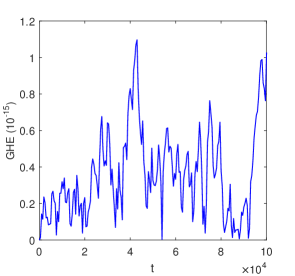
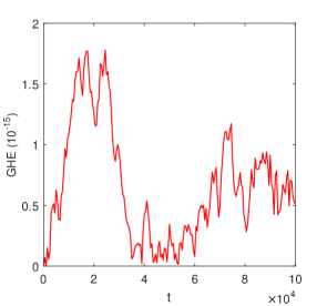
Figure 1: The global energy errors (GHE) of the reference solutions with $c=10^{1/2}$ (left) and $c=10$ (right).

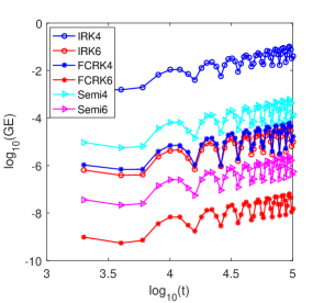
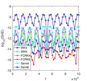
Figure 2: The global errors (GE) and energy errors (GHE) with $h=1$ and $c=10^{1/2}$.

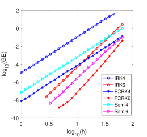
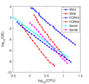
Figure 3: The numerical convergence orders and efficiency curves with $c=10^{1/2}$.

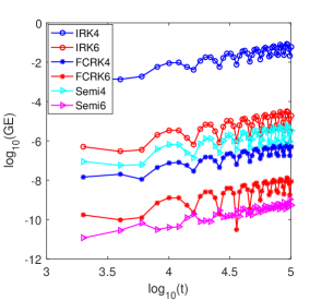
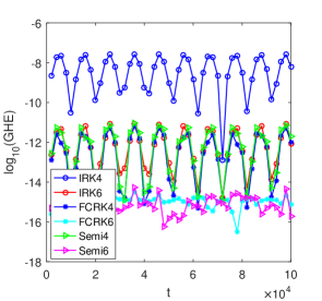
Figure 4: The global errors (GE) and energy errors (GHE) with $h=1$ and $c=10$.

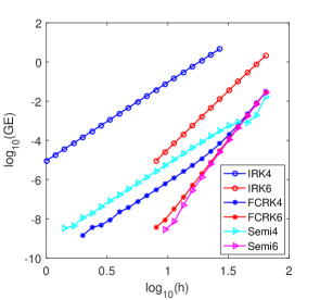
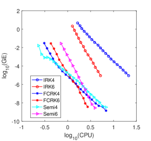
Figure 5: The numerical convergence orders and efficiency curves with $c=10$.

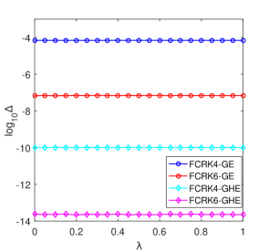
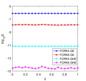
Figure 6: The dependence of global (energy) errors on the free parameter $\lambda$ with $h=10$ and $c=10^{1/2}$ (left) or $c=10$ (right).

In the numerical experiments, we take the initial values as follows: $\bm{Q}=(25.34,0,0)$, $\bm{P}=(0,0.18,0)$, $\bm{\theta}=(1.2490,0.6202)$, and $\bm{\xi}=(0.0445,0.0705)$. The spin magnitudes are set as $\Lambda_{1}=0.0479$ and $\Lambda_{2}=0.6104$. The mass ratio is $\beta=0.28$. Moreover, we use the geometric unit $G=M=1$, under which the parameter $c$ should be readjusted to denote different PN effects. Usually, a large value of $c$ thus a small $\varepsilon$ indicates a weak PN effect.

In this paper, we select six symplectic methods to make the comparison, i.e., the classical Gauss collocation methods IRK4 and IRK6, the symplectic GFCRK methods FCRK4 and FCRK6 respectively based on IRK4 and IRK6, and the semi-explicit mixed symplectic methods Semi4 and Semi6. Moreover, the free parameter $\lambda$ of the GFCRK method is fixed as $1/2$ unless otherwise stated.

In addition, we need reference solutions of very high accuracy to measure the global error of the tested numerical methods. Since the exact solutions cannot be obtained in general, we regard the numerical solutions obtained by the eighth-order Gauss symplectic collocation method with tiny stepsize as the reference solutions. The energy errors for the two cases $c=10^{1/2}$ and $c=10$ are presented in Fig. 1, which shows the high accuracy of the reference solutions.

For the case of $c=10^{1/2}$, the global errors and energy errors of the six tested symplectic methods are shown in Fig. 2, from which three notable points are observed. Firstly, the global errors increase linearly with respect to time, while the energy errors are uniformly bounded. This point clearly coincides with the property of symplectic methods. Secondly, the GFCRK methods FCRK4 and FCRK6 and the semi-explicit methods Semi4 and Semi6 perform better than the fully implicit symplectic methods, i.e., IRK4 and IRK6, which shows the superiority of taking the advantage of the small parameter $\varepsilon$ in the designing of numerical integrators. Thirdly, the GFCRK methods FCRK4 and FCRK6 present a higher accuracy than the corresponding semi-explicit methods Semi4 and Semi6.

The numerical convergence orders and efficiency curves of the tested symplectic methods with $T=10^{5}$ are shown in Fig. 3. The slopes of the curves in the left panel of Fig. 3 are3.98, 5.97, 4.02, 6.53, 3.98, and 5.84 respectively for IRK4, IRK6, FCRK4, FCRK6, Semi4, and Semi6, which are in well accordance with the theoretical convergence orders 4 and 6. The efficiency curves of global errors versus CPU time (in seconds) shown in the right panel of Fig. 3 means that the GFCRK method has the highest efficiency among symplectic methods of the same order. We also note that the sixth-order GFCRK method FCRK6 is most efficient among all the tested methods.

The similar results corresponding to Fig. 2 and Fig. 3 but with $c=10$ are respectively presented in Fig. 4 and Fig. 5. A slight difference between Fig. 4 and Fig. 2 is that Semi6 behaves better with a smaller global errors than FCRK6 once $c=10$. The slops in the right panel of Fig. 5 are 3.99, 5.96, 4.63, 7.29, 3.87, and 7.81 respectively for IRK4, IRK6, FCRK4, FCRK6, Semi4, and Semi6, where FCRK6 and Semi6 give a surprising superconvergence as the slops are evidently larger than the theoretical value 6. Besides the similar result that the GFCRK method of the same order is more efficient than the semi-explicit method and the semi-explicit method is more efficient than the RK method, it is also observed from the right panel of Fig. 5 that the high-order GFCRK/semi-explicit method intersects the low-order GFCRK/semi-explicit method at some points, which indicates that the high-order method is preferred under a high accuracy requirement while the low-order method will be more efficient under a low accuracy requirement.

A further efficiency comparison with constant stepsizes among the six symplectic methods are presented Table 1 and Table 2, where two different cases of $c=10^{1/2}$ and $c=10$ are tested. It is observed from the two tables that under a constant stepsize, the Semi4 consumes the least CPU time among all the three fourth-order method, while the CPU time of FCRK4 is between IRK4 and Semi4. As to the sixth-order method, FCRK6 consumes evidently less CPU time than IRK6 and Semi6 in both the two cases of $c=10^{1/2}$ and $c=10$, while Semi6 consumes more time than IRK6 for $c=10^{1/2}$ but less time than IRK6 for $c=10$. That is, a small parameter $\varepsilon$ will decrease the computational complexity of the GFCRK method and the semi-explicit symplectic method. Overall, these two tables along with the right panels of Fig. 3 and Fig. 5 show that although the fourth-order FCRK4 may consume more time than the semi-explicit Semi4 in a single stepsize, the GFCRK methods are more efficient than semi-explicit mixed symplectic methods, i.e., consume less CPU time under a certain accuracy requirement for the numerical solutions.

We finally investigate the dependence of the global errors or energy errors on the free parameter $\lambda$ in Fig. 6. It is observed from this figure that the value of $\lambda$ hardly takes influence on the numerical performance of the GFCRK method. Therefore, the values $0$ and $1$ are preferred for the parameter $\lambda$ due to the slightly less computational amount than any other values as analyzed in Section 3.2 if the time-symmetry is not necessarily required for the GFCRK method.

Table 1: CPU time (in seconds) with $c=\sqrt{10}$ and $T_{end}=10^{5}$.

h=1 h=2 h=4 h=8 h=16

IRK4 22.2378 12.2425 6.9827 3.9933 2.3592

IRK6 31.7401 17.6606 9.3325 5.4190 3.3086

FCRK4 16.4997 8.8679 4.4699 2.3934 1.3537

FCRK6 24.9059 12.6779 6.3993 3.4547 1.8922

Semi4 13.1429 6.5675 3.6056 1.9640 1.0785

Semi6 39.2345 20.0783 11.0060 6.0831 3.3147

Table 2: CPU time (in seconds) with $c=10$ and $T_{end}=10^{5}$.

h=1 h=2 h=4 h=8 h=16

IRK4 21.5280 11.9129 6.7989 3.8822 2.2873

IRK6 30.9710 17.1126 9.0580 5.2335 3.2029

FCRK4 13.4741 6.8259 3.3717 1.9109 1.0972

FCRK6 19.0491 9.5381 5.0146 2.7411 1.6891

Semi4 9.6276 4.9270 2.7426 1.5781 0.7884

Semi6 28.8026 15.2954 8.7561 4.7148 2.3924

5 Conclusion

The long-term reliability of numerical solutions for Hamiltonian systems usually requires the use of symplectic methods, which possess the advantages of linear growth of global errors and near preservation of first integrals. Meanwhile, the nonseparability of the post-Newtonian Hamiltonian system of compact objects makes the available symplectic methods to be implicit. On noting the fact that the PN Hamiltonian could be split into a dominant Newtonian part and a PN perturbation part, we focused on the efficient numerical simulation of PN Hamiltonian systems by studying the FCRK method, where the change of variable composed by the phase flow of the Kepler problem is employed. In this paper, we first presented the generalized FCRK method with a free parameter to the PN Hamiltonian system. Then, we discussed the properties, such as the time-symmetry, the symplecticity, the convergence, and the implementation of the GFCRK method. In particular, we compared the symplectic GFCRK method with the mixed symplectic method. Finally, we conducted numerical experiments for the 2PN Hamiltonian of spinning compact binaries with six implicit symplectic methods, i.e., the Gauss-type methods IRK4 and IRK6, the GFCRK methods FCRK4 and FCRK6 that are respectively based on IRK4 and IRK6, and the mixed symplectic methods Semi4 and Semi6. Numerical results showed that the symplectic GFCRK method is always more efficient than the Gauss-type symplectic method and the mixed symplectic method of the same order by consuming less CPU time under the prescribed accuracy requirement. Moreover, we found that the free parameter $\lambda$ hardly takes influence on the numerical performance of the GFCRK method. This indicates an additional degree of freedom for the GFCRK method, which potentially enables us to use this degree of freedom to design GFCRK method that preserves the energy or other first integrals of the system.

References

- Baker et al. [2007] J.G. Baker, J.R. van Meter, S.T. McWilliams, J. Centrella, B.J. Kelly, Consistency of post-Newtonian waveforms with numerical relativity, Phys. Rev. Lett. 99, 181101 (2007)
- Wu & Zhong [2011] X. Wu, S. Zhong, Regular dynamics of canonical post-Newtonian Hamiltonian for spinning compact binaries with next-to-leading order spin-orbit interactions, Gen. Relativ. Gravit. 43, 2185–2198 (2011)
- Wu & Huang [2015] X. Wu, G. Huang, Ruling out chaos in comparable mass compact binary systems with one body spinning, Mon. Not. R. Astron. Soc. 452, 3167–3178 (2015)
- Wu et al. [2015] X. Wu, L. Mei, G. Huang, S. Liu, Analytical and numerical studies on differences between Lagrangian and Hamiltonian approaches at the same post-Newtonian order, Phys. Rev. D 91, 024042 (2015)
- Hairer et al. [1987] E. Hairer, S.P. Nørsett, G. Wanner, Solving Ordinary Differential Equations I: Non-Stiff Systems. (Springer Berlin, 1987)
- Calvo & Hairer [1995] M.P. Calvo, E. Hairer, Accurate long-term integration of dynamical systems, Appl. Numer. Math. 18, 95–105 (1995)
- Hairer, Lubich & Wanner [2006] E. Hairer, C. Lubich, G. Wanner, Geometric Numerical Integration: Structure-Preserving Algorithms for Ordinary Differential Equations, 2nd ed. (Springer Berlin, 2006)
- Feng & Qin [2010] K. Feng, M. Qin, Symplectic Geometric Algorithms for Hamiltonian Systems, (Springer/Zhejiang Science & Technology Press, Berlin/Hangzhou, 2010)
- Sanz-Serna [1988] J. M. Sanz-Serna, Runge–Kutta schemes for Hamiltonian systems, BIT Numer. Math. 28, 877–883 (1988)
- Ruth [1983] R.D. Ruth, A canonical integration technique, IEEE Trans. Nucl. Sci. 30, 2669–2671 (1983)
- Forest & Ruth [1990] E. Forest, R.D. Ruth, Fourth-order symplectic integration, Phys. D 43, 105–117 (1990)
- Wisdom & Holman [1991] J. Wisdom, M. Holman, Symplectic maps for the n-body problem, Astron. J. 102, 1528–1538 (1991)
- Chin [1997] S.A. Chin, Symplectic integrators from composite operator factorizations, Phys. Lett. A 226, 344–348 (1997)
- Chin [2007] S.A. Chin, Physics of symplectic integrators: Perihelion advances and symplectic corrector algorithms, Phys. Rev. E 75, 036701 (2007)
- Omelyan, Mryglod & Folk [2007] I.P. Omelyan, I.M. Mryglod, R. Folk, Construction of high-order force-gradient algorithms for integration of motion in classical and quantum systems, Phys. Rev. E 66, 026701 (2002)
- McLachlan [1995] R.I. McLachlan, Composition methods in the presence of small parameters, BIT Numer. Math. 35, 258–268 (1995)
- Chambers & Murison [2000] J.E. Chambers, M.A. Murison, Pseudo-high-order symplectic integrators, Astron. J. 119, 425 (2000)
- Laskar & Robutel [2001] J. Laskar, P. Robutel, High order symplectic integrators for perturbed Hamiltonian systems, Celest. Mech. Dyn. Astr. 80, 39–62 (2001)
- Farrés et al. [2013] A. Farrés, J. Laskar, S. Blanes, F. Casas, J. Makazaga, A. Murua, High precision symplectic integrators for the Solar System, Celest. Mech. Dyn. Astr. 116, 141–174 (2013)
- Lubich, Walther & Brügmanngmann [2010] C. Lubich, B.Walther, B. Brügmann, Symplectic integration of post-Newtonian equations of motion with spin, Phys. Rev. D 81, 104025 (2010)
- Zhong et al. [2010] S.Y. Zhong, X. Wu, S.Q. Liu, X.F. Deng, Global symplectic structure-preserving integrators for spinning compact binaries, Phys. Rev. D 82, 124040 (2010)
- Mei, Wu & Liu [2013] L. Mei, X. Wu, F. Liu, On preference of Yoshida construction over Forest–Ruth fourth-order symplectic algorithm, Eur. Phys. J. C 73, 2413 (2013)
- Mei & Huang [2024] L. Mei, L. Huang, Explicit near-symplectic integrators for post-Newtonian Hamiltonian systems, Eur. Phys. J. C 84, 76 (2024)
- Pihajoki [2015] P. Pihajoki, Explicit methods in extended phase space for inseparable Hamiltonian problems, Celest. Mech. Dyn. Astr. 121, 211–231 (2015)
- Tao [2016] M. Tao, Explicit symplectic approximation of nonseparable Hamiltonians: Algorithm and long time performance, Phys. Rev. E 94, 043303 (2016)
- Liu et al. [2016] L. Liu, X. Wu, G. Huang, F. Liu, Higher order explicit symmetric integrators for inseparable forms of coordinates and momenta, Mon. Not. R. Astron. 459, 1968–1976 (2016)
- Jayawardana & Ohsawa [2023] B. Jayawardana, T. Ohsawa, Semiexplicit symplectic integrators for non-separable Hamiltonian systems, Math. Comp. 92, 251–281 (2023)
- Antoñana, Makazaga & Murua [2017] M. Antoñana, J. Makazaga, A. Murua, New integration methods for perturbed ODEs based on symplectic implicit Runge–Kutta schemes with application to solar system simulations, J. Sci. Comput. 76, 630–650, (2018)
- Damour, Jaranowski & Schäfer [2001] T. Damour, P. Jaranowski, G. Schäfer, Equivalence between the ADM-Hamiltonian and the harmonic-coordinates approaches to the third post-Newtonian dynamics of compact binaries, Phys. Rev. D 63, 044021 (2001)
- de Andrade, Blanchet & Faye [2001] V.C. de Andrade, L. Blanchet, G. Faye, Third post-Newtonian dynamics of compact binaries: Noetherian conserved quantities and equivalence between the harmonic-coordinate and ADM-Hamiltonian formalisms, Classical. Quant. Grav. 18, 753 (2001)
- Levi & Steinhoff [2014] M. Levi, J. Steinhoff, Equivalence of ADM Hamiltonian and Effective Field Theory approaches at next-to-next-to-leading order spin1-spin2 coupling of binary inspirals, J. Cosmol. Astropart. Phys. 12, 003 (2014)
- Huang & Wu [2014] G. Huang, X. Wu, Dynamics of the post-Newtonian circular restricted three-body problem with compact objects, Phys. Rev. D 89, 124034 (2014)
- Dubeibe, Lora-Clavijo & Gonzalez [2017] F.L. Dubeibe, F.D. Lora-Clavijo, G.A. Gonzalez, On the conservation of the Jacobi integral in the post-Newtonian circular restricted three-body problem, Astrophys. Space Sci. 362, 97 (2017)
- Huang, Mei & Huang [2018] L. Huang, L. Mei, S. Huang, Non-truncated strategy to exactly integrate the post-Newtonian Lagrangian circular restricted three-body problem, Eur. Phys. J. C 78, 814 (2018)
- Spyrou [1975] N. Spyrou, The N-body problem in general relativity, Astrophys. J. 197, 725–743 (1975)
- Quinn, Tremaine & Duncan [1991] T.R. Quinn, S. Tremaine, M. Duncan, A three million year integration of the earth’s orbit, Astron. J. 101, 2287–2305 (1991)
- Chu [2009] Y.Z. Chu, N-body problem in general relativity up to the second post-Newtonian order from perturbative field theory, Phys. Rev. D 79, 044031 (2009)
- Buonanno, Chen & Damour [2006] A. Buonanno, Y. Chen, T. Damour, Transition from inspiral to plunge in precessing binaries of spinning black holes, Phys. Rev. D 74, 104005 (2006)
- Nagar [2011] A. Nagar, Effective one-body Hamiltonian of two spinning black holes with next-to-next-to-leading order spin-orbit coupling, Phys. Rev. D 84, 084028 (2011)
- Lhotka & Celletti [2015] C. Lhotka, A. Celletti, The effect of Poynting–Robertson drag on the triangular Lagrangian points, Icarus 250, 249 (2015)
- Huang & Mei [2019] L. Huang, L. Mei, Symplectic integrators for post-Newtonian Lagrangian dynamics, Phys. Rev. D 100, 024057 (2019)
- Wu & Xie [2010] X. Wu, Y. Xie, Symplectic structure of post-Newtonian Hamiltonian for spinning compact binaries, Phys. Rev. D 81, 084045 (2010)
- Lawson [1967] J.D. Lawson, Generalized Runge–Kutta processes for Stable Systems with large Lipschitz constants, SIAM J. Numer. Anal. 4, 372–380 (1967)
- Celledoni, Cohen & Owren [2008] E. Celledoni, D. Cohen, B. Owren, Symmetric exponential integrators with an application to the cubic Schrödinger Equation, Found. Comput. Math. 8, 303–317 (2008)
- Mei & Wu [2017] L. Mei, X. Wu, Symplectic exponential Runge–Kutta methods for solving nonlinear Hamiltonian systems, J. Comput Phys. 338, 567–584 (2017)
- Yoshida [1990] H. Yoshida, Construction of higher order symplectic integrators, Phys. Lett. A 150, 262–268 (1990)