Interpretating Pulsar Timing Array data of Gravitational Waves with Ekpyrosis-Bouncing Cosmology

Abstract

Recent pulsar timing array (PTA) experiments have reported strong evidence of the stochastic gravitational wave background (SGWB). If interpreted as primordial Gravitational Waves (pGWs), the signal favors a strongly blue-tilted spectrum. On the other hand, the Ekpyrosis-bouncing cosmology with a strongly blue-tilted GW spectrum, i.e., $n_{T}\simeq 2$, offers a potential explanation for the observed SGWB signal. In this paper, we construct a concrete Ekpyrosis-bouncing model, and show its capacity to intepret the PTA result without pathologies. Both tensor and scalar perturbations are analysed with constraints from the current observations.

1 Introduction

Bouncing cosmology is an important topic in the early universe cosmology [1]. The standard paradigm of the early universe equipped with inflation suffers from the initial singularity problem [2, 3] (see [4, 5] for recent development) and the trans-Planckian problem [6, 7]. In light of that, bouncing cosmology is motivated to evade the conceptual puzzles in inflationary cosmology. Moreover, bouncing cosmology can also solve the horizon, flatness and monopole problems, as well as providing a natural explanation for the formation of the large scale structure [8].

Recently, pulsar timing array (PTA) collaborations, including NANOGrav [9, 10], EPTA [11], PPTA [12], and CPTA [13], have reported strong evidence for an isotropic stochastic GW background with a strain amplitude of order $\mathcal{O}(10^{-15})$ at the reference frequency $f=1\,\textnormal{yr}^{-1}$. See Ref. [14, 15, 16, 17, 18, 19, 20, 21, 22, 23, 24, 25, 26, 27, 28, 29, 30, 31, 32, 33, 34, 35, 36, 37, 38, 39, 40, 41, 42, 43, 44, 45, 46, 47, 48, 49, 50, 51, 52, 53, 54, 55, 56, 57, 58, 59, 60, 61, 62, 63, 64] for interpretations of PTA results. The PTA result strongly supports a blue tensor spectrum with $n_{T}=1.8\pm 0.3$ [65]. It is well-known that, the canonical inflation scenario predicts a nearly scale invariant primordial tensor spectra. On the other hand, the Ekpyrosis bouncing cosmology [67, 68], predict a blue tensor spectra with a spectral index $2<n_{T}<3$ (see [69] for exceptions). Therefore, the recent PTA result might be a potential hint for the Ekpyrosis bouncing cosmology. See concrete models of Ekpyrosis bouncing cosmology in Ref. [70, 71, 72, 73, 74, 75, 76, 77, 78, 79, 80].

In [81], we conduct a prelimilary check on the possibility to explain the PTA data by the primordial gravitational wave (PGW) signal in non-singular cosmology. It is found that, although our toy Genesis-inflation model can potentially generate a stochastic gravitational wave background (SGWB) capable for PTA result, there are issues, such as a trans-Planckian problem and an oversized scalar perturbation, to be addressed in details. Therefore, it is important to study the above issue in a concrete realization.

In this paper, we will provide a concrete realization of non-singular bouncing cosmology capable with PTA observations. In bouncing scenario, the universe starts with a contraction epoch with Hubble parameter $H<0$. After a bouncing epoch where $H$ transits from negative to positive, the universe enters into an expansion epoch. We will adopt an Ekpyrotic contraction epoch, for not only the blue tensor spectra, but also its robustness against anisotropic stress and initial conditions [82]. Unfortunately, the Ekpyrotic contraction epoch also predicts a blue-tilted scalar spectra, which is inconsistent with observations. Thus, we follow the curvaton mechanism to acquire a nearly scale-invariant scalar spectra on CMB scales, while keeping the tensor spectra blue [83]. Under the above guidance, we construct our model with a concrete action, and show that the observed PTA signals can be predicted with suitable choices of model parameters without the over-production of primordial fluctuations.

The paper is organized as follows. We present our model and the description of background evolution in Sec. 2. We analyze the tensor and scalar perturbation in Sec. 3 and 5, respectively. A numerical investigation of the tensor power spectrum and its connection to PTA observation is presented in Sec. 4. We finally conclude in Sec. 6. Throughout this paper, we adopt the $(-,+,+,+)$ convention. The scalar field $\phi$ is set to be dimensionless, so the canonical kinetic term $X$, defined as $X\equiv-(1/2)g^{\mu\nu}\nabla_{\mu}\phi\nabla_{\nu}\phi$, is of dimension $[M]^{2}$. We use an overdot to denote the differentiation with respect to cosmic time $t$, and a prime to denote the differentiation with respect to conformal time $\tau\equiv dt/a$.

2 Model and background

2.1 Action

The generic action is taken to be

$$S=\int d^{4}x\sqrt{-g}\left[M_{p}^{2}\frac{R}{2}+K(\phi,X)+\mathcal{L}_{\textnormal{EFT}}+\mathcal{L}_{\sigma}\right]~{},$$ (2.1)

where $R/2$ is the Einstein-Hilbert action. The action (2.1) is composed by three part, which we shall explain below.

The k-essence action $K(\phi,X)$ is responsible for the background dynamics. We assume that the universe starts with an Ekpyrotic contraction epoch at $\phi\ll-1$, and finally evolves into an radiation-dominated expansion epoch at $\phi\gg 1$. This suggests the following asymptotic behavior of $K$:

$$\lim_{\phi\to-\infty}K(\phi,X)=X+2V_{0}e^{\sqrt{\frac{2}{q}}\phi}~{};~{}\lim_{\phi\to\infty}K(\phi,X)=X^{2}~{}.$$ (2.2)

Moreover, during the bouncing epoch, NEC is violated. We will use a ghost-condensate type action [84], i.e. $-X+X^{2}$, to violate NEC. Therefore, the k-essence action shall take the form

$$K(\phi,X)=[1-g(\phi)]M_{p}^{2}X+\beta_{2}X^{2}-M_{p}^{4}V(\phi)~{},$$ (2.3)

with $g$ being the smooth top-hat function

$$g(\phi) =\beta_{1}\left[\frac{1+\tanh\lambda_{1}(\phi-\phi_{-})}{2}\right]\left[\frac{1+\tanh\lambda_{2}(\phi_{+}-\phi)}{2}\right]$$

$$+\frac{1+\tanh\lambda_{4}(\phi-\phi_{+})}{2}~{},~{}\phi_{-}<\phi_{+}~{},$$ (2.4)

and a potential

$$V(\phi)=-2V_{0}e^{\sqrt{\frac{2}{q}}\phi}\frac{1-\tanh\lambda_{3}(\phi-\phi_{-})}{2}~{},$$ (2.5)

with the restriction $\lambda_{3}>1/\sqrt{2q}$. One may check that in the ansatz, (2.3) along with (2.1) and (2.5), the asymptotic behavior (2.2) is satisfied (the potential $V(\phi)$ is exponentially suppressed so that the action is dominated by the $X^{2}$ term when $\phi>\phi_{+}$). Besides, when $\phi_{-}<\phi<\phi_{+}$, the action (2.3) becomes

$$K(\phi,X)\simeq(1-\beta_{1})M_{p}^{2}X+\beta_{2}X^{2}-M_{p}^{4}V(\phi)~{}.$$ (2.6)

which permits an NECV as long as $\beta_{1}>1$.

There will be ghost or gradient instability problems in the generic bouncing models within the framework of Horndeski theory [85, 86, 87]. The simplest way to evade the instabilities is to introduce an EFT operator in the context of non-singular cosmology [88, 89, 90, 91] (alternative approaches can be found in [92, 93, 94, 95, 79, 96, 97, 98, 99, 100, 101, 102, 103, 80]). Since the EFT operator changes the scalar sound speed $c_{s}^{2}$ only, and has no impact on the background dynamics and tensor perturbations, we may simply use it to resolve the instability problem for bouncing cosmology, and don’t need to worry about its contribution to both the background evolution and linear perturbations.

However, the Ekpyrotic contraction period will generate a blue-tilted scalar power spectrum [104, 105, 106, 107, 108, 109]. Therefore, it is useful to introduce a curvaton field $\sigma$ coupled to the scalar field $\phi$, which can lead to the desired scale-invariant scalar power spectrum, while leaving the bouncing background unchanged [83, 110, 111, 112, 113, 114, 70]. As shown explicitly in [83], we can adopt the follwing action for curvaton:

$$\mathcal{L}_{\sigma}=-\frac{M_{p}^{2}}{2}f^{2}e^{\sqrt{2/q}\phi}(\partial\sigma)^{2}~{},$$ (2.7)

acquiring a scale-invariant scalar power spectrum which is constant in time. Here, $f$ is a dimensionless parameter. Unfortunately, in the simple set (2.7), the curvaton field will be dominant in the expansion stage where $\phi\gg 1$. In view of that, a realistic choice of curvaton action can be

$$\mathcal{L}_{\sigma}=-M_{p}^{2}f^{2}\frac{\sqrt{\frac{2}{q}}+\phi e^{\sqrt{\frac{q}{2}}\phi}}{e^{-\sqrt{\frac{q}{2}}\phi}+\phi^{2}e^{\sqrt{\frac{q}{2}}\phi}}(\partial\sigma)^{2}~{},$$ (2.8)

which exactly has the asymptotic form (2.7) when $\phi\ll 1$. At the expansion stage, the action (2.8) approximates to $\mathcal{L}_{\sigma}\propto\phi^{-1}(\partial\sigma)^{2}$, which we shall explain in details in Sec. 5.3. Besides, one may check that the denominator and numerator in (2.8) is always positive.

In the following, we will start with the action (2.1), along with (2.3) and (2.8), to pursue its background and perturbation evolutions and to see how the primordial GWs can meet with the PTA data.

2.2 Equations of motion for background

According to (2.1), (2.3) and (2.8), the Friedmann’s equations are

$$3H^{2}M_{p}^{2}=\rho=\frac{1}{2}(1-g)M_{p}^{2}\dot{\phi}^{2}+\frac{3}{4}\beta_{2}\dot{\phi}^{4}+M_{p}^{4}V(\phi)+\frac{M_{p}^{2}f^{2}}{2\cosh(\sqrt{2/q}\phi)}\dot{\sigma}^{2}~{},$$ (2.9)

$$-2\dot{H}M_{p}^{2}=\rho+p=(1-g)M_{p}^{2}\dot{\phi}^{2}+\beta_{2}\dot{\phi}^{4}+\frac{M_{p}^{2}f^{2}}{\cosh(\sqrt{2/q}\phi)}\dot{\sigma}^{2}~{}.$$ (2.10)

Since we now have two fields, we need one additional dynamical equation. We obtain the dynamics of $\sigma$ by varying the action (2.1) with respect to $\sigma$:

$$\ddot{\sigma}+\dot{\sigma}\frac{d}{dt}\left[\ln\left(a^{3}M_{p}^{2}f^{2}\cosh^{-1}(\sqrt{2/q}\phi)\right)\right]=0~{}.$$ (2.11)

Apart from the constant solution $\dot{\sigma}=0$, there’s another branch of solution

$$\dot{\sigma}a^{3}M_{p}^{2}f^{2}\cosh^{-1}(\sqrt{2/q}\phi)=\textnormal{const}~{}.$$ (2.12)

Before proceeding, we shall examine whether the curvaton field has negligible contributions to the background dynamics. In the contraction epoch, we have $\cosh^{-1}(\sqrt{2/q}\phi)\simeq e^{\sqrt{2/q}\phi}$, so the curvaton has no significant contribution to the background, as proved in [83]. In the radiation dominated epoch, we have $\dot{\phi}\propto t^{-1/2}$ such that $\phi$ grows as $t^{1/2}$. Thus $\dot{\sigma}\propto t^{-1}$ according to (2.8) and the energy density of curvaton field evolves as $\rho_{\sigma}\propto\phi^{-1}\dot{\sigma}^{2}=t^{-5/2}$. So $\rho_{\sigma}$ decays more rapidly than the background energy density and there is no backreaction problem in the radiation dominated epoch. In both cases, the curvaton field has no change to introduce a large back-reaction to the background.

Finally, it would be useful to write down the dynamical equation of $\phi$ in the numerical process. Since we’ve omitted the contributions of the curvaton field on the background level, the equation simplifies to

$$\left[(1-g)M_{p}^{2}+3\beta_{2}\dot{\phi}^{2}\right]\ddot{\phi}+3H\dot{\phi}\left((1-g)M_{p}^{2}+\beta_{2}\dot{\phi}^{2}\right)+M_{p}^{4}V^{\prime}(\phi)-\frac{M_{p}^{2}}{2}g^{\prime}(\phi)\dot{\phi}^{2}=0~{}.$$ (2.13)

2.3 Background evolution in different epochs

In the far past $\phi\ll-1$ and $\dot{\phi}\ll M_{p}$ (so that the $X^{2}$ term is subdominate to the $X$ term), with the help of (2.2), the Friedmann equations (2.9), (2.10) become

$$3H^{2}M_{p}^{2}=\frac{1}{2}M_{p}^{2}\dot{\phi}^{2}-2V_{0}M_{p}^{4}e^{\sqrt{\frac{2}{q}}\phi}~{},~{}-2\dot{H}=\dot{\phi}^{2}~{},$$ (2.14)

which gives the Ekpyrotic attractor solution

$$\phi\simeq-\sqrt{\frac{q}{2}}\ln\left[\frac{2V_{0}M_{p}^{2}t^{2}}{q(1-3q)}\right]~{},~{}\dot{\phi}=\frac{\sqrt{2q}}{-t}~{};~{}H=\frac{q}{t}<0~{}.$$ (2.15)

The effective equation-of-state (EoS) parameter in the Ekpyrotic contraction epoch is solely determined by the parameter $q$: $w_{c}=-1+2/(3q)$. The spacetime geometry evolves accordingly:

$$a(\tau)=a_{-}\left(\frac{\tau_{e}-\tau}{\tau_{e}-\tau_{-}}\right)^{\frac{q}{1-q}}~{},~{}\mathcal{H}=\frac{-q}{(1-q)(\tau_{e}-\tau)}<0~{},$$ (2.16)

where $\tau\equiv\int dt/a$ is the conformal time and $\mathcal{H}=aH$ is the conformal Hubble parameter. $\tau_{-}$ is the end time of the contraction epoch and $a_{-}\equiv a(\tau_{-})$ is the corresponding scale factor. Finally, $\tau_{e}>\tau_{-}$ is an integration constant. It is convenient to have the relation between $t$ and $\tau$:

$$t=\int a(\tau)d\tau=-a_{-}(1-q)\left[\frac{(\tau_{e}-\tau)}{(\tau_{e}-\tau_{-})^{q}}\right]^{\frac{1}{1-q}}<0~{},$$ (2.17)

up to an integration constant.

The evolution of fluctuations in bouncing epoch is generically involved. Fortunately, the duration of the bouncing epoch is usually taken to be short. For example, in [121] it is pointed out that the sourced anisotropy in the bouncing epoch grows exponentially. Thus a short bounce is favored for the model to be free from anisotropic stress problem. In this case, the bouncing epoch can be parametrized in the following

$$\mathcal{H}\simeq\alpha^{2}(\tau-\tau_{B})~{},~{}a=a_{B}e^{\frac{1}{2}\alpha^{2}(\tau-\tau_{B})^{2}}~{},~{}\tau_{-}<\tau<\tau_{+}~{},$$ (2.18)

where $\tau_{B}$ is an integration constant and $\tau_{+}$ is the end of bouncing epoch (or equivalently, the beginning of expanding epoch). The validation of the linear approximation requires $|\alpha(\tau-\tau_{B})|<1$.

While the parameterization (2.18) can be understood as a taylor expansion around the bouncing point, the dynamics of scalar field $\phi$ in bouncing phase is more involved. In [72] the authors present an approximated formulae

$$\dot{\phi}\simeq M_{p}\sqrt{\frac{2(\beta_{1}-1)}{3\beta_{2}}}e^{-t^{2}/T^{2}}~{},$$ (2.19)

with $T$ a free parameter, which roughly equals to a quarter of the duration of bouncing phase. The validation of (2.19) is examined by the authors in [72] by numerics. We will use (2.19) to describe the dynamics of $\phi$ in bouncing phase in the rest of the paper.

After the bouncing epoch, the universe enters into an expansion phase. The Lagrangian of $\phi$ is $K(\phi,X)=X^{2}$, so that $\rho=3X^{2}$ and $p=X^{2}$ and the Equation-of-state parameter for $\phi$ becomes $w_{\phi}=1/3$. The universe will then be radiation-dominated. The corresponding background dynamics becomes

$$a=a_{+}\frac{\tau-\tilde{\tau}}{\tau_{+}-\tilde{\tau}}~{},~{}\mathcal{H}=\frac{1}{\tau-\tilde{\tau}}~{}.$$ (2.20)

2.4 Matching condition

In order to maintain the continuity of $a$ and ${\cal H}$, the background dynamics in each epoch can be furtherly matched by the junction condition at the transition surface $\tau=\tau_{-}$ and $\tau=\tau_{+}$. Firstly, we set the bouncing point $H=0$ to be the zero point of $\tau$, (i.e., $\tau_{B}=0$), so that $\tau_{-}<0$, $\tau_{+}>0$ and

$$\mathcal{H}=\alpha^{2}\tau~{},~{}a=a_{B}e^{\frac{1}{2}\alpha^{2}\tau^{2}}~{},~{}\tau_{-}<\tau<\tau_{+}~{},$$ (2.21)

the continuity at $\tau=\tau_{-}$ gives

$$\tau_{e}=\tau_{-}-\frac{q}{(1-q)\alpha^{2}\tau_{-}}~{},$$ (2.22)

and the continuity at $\tau=\tau_{+}$ gives $\tilde{\tau}=\tau_{+}-(\alpha^{2}\tau_{+})^{-1}$. For the sake of simplicity, let’s work in a symmetric bounce, i.e., $|\tau_{-}|=\tau_{+}$. Then we have $a_{-}=a_{+}=a_{B}e^{\alpha^{2}\tau_{+}^{2}/2}$. Implemented with those conditions, we summarize the evolution of scale factor

$$a(\tau)=\left\{\begin{array}[]{cl}&a_{B}e^{\frac{1}{2}\alpha^{2}\tau_{+}^{2}}\left[1+\frac{1-q}{q}\alpha^{2}|\tau_{-}|(\tau_{-}-\tau)\right]^{\frac{q}{1-q}}~{},~{}\tau<\tau_{-}~{},\\ \\ &a_{B}e^{\frac{1}{2}\alpha^{2}\tau^{2}}~{},~{}\tau_{-}<\tau<\tau_{+}~{},\\ \\ &a_{B}e^{\frac{1}{2}\alpha^{2}\tau_{+}^{2}}\left[1+\mathcal{H}_{+}(\tau-\tau_{+})\right]~{},~{}\tau>\tau_{+}~{}.\end{array}\right.$$ (2.23)

and of conformal Hubble parameter

$$\mathcal{H}(\tau)=\left\{\begin{array}[]{cl}&\alpha^{2}\tau_{-}\left[1+\frac{1-q}{q}\alpha^{2}|\tau_{-}|(\tau_{-}-\tau)\right]^{-1}~{},~{}\tau<\tau_{-}~{},\\ \\ &\alpha^{2}\tau~{},~{}\tau_{-}<\tau<\tau_{+}~{},\\ \\ &\alpha^{2}\tau_{+}\left[1+\alpha^{2}\tau_{+}(\tau-\tau_{+})\right]^{-1}~{},~{}\tau>\tau_{+}~{}.\end{array}\right.$$ (2.24)

The background value is thus fixed by four parameters: $\alpha$, $\tau_{+}$, $a_{B}$ and $q$.

We numerically evaluate the background dynamics using the following parameter set $\beta_{1}=1.1$, $\beta_{2}=1$, $\phi_{-}=-0.1$, $\phi_{+}=3.7$, $V_{0}=10^{-1}$, $q=0.005$, and present the evolution of Hubble parameters in Fig. 1. In the figure, the Hubble parameter goes from below zero to above zero, indicating that bounce indeed occurs. While before the bounce the EoS is very large as in the Ekpyrosis phase $w=-1+2/(3q)$, after the bounce the universe enters a radiation-dominated era where the EoS is nearly $1/3$. Note that all model parameters are normalized to be dimensionless.

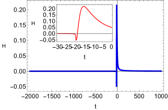
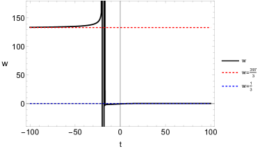
Figure 1: Sketch of Hubble parameter and Equation-of-state parameter near the bouncing phase.

3 Tensor perturbations

3.1 Generic formalism

Now we turn to the tensor perturbations generated in our model. The quadratic action of tensor perturbation is

$$S_{2,T}=\int d\tau d^{3}x\frac{a^{2}}{8}M_{p}^{2}\left[\gamma_{ij}^{\prime 2}-c_{T}^{2}(\partial\gamma_{ij})^{2}\right]~{},$$ (3.1)

where $\gamma_{ij}$ represents the tensor perturbation which is dimensionless. Here for simplicity, we don’t distinguish the polarization modes for the tensor sector. Since the matter sector is minimally coupled to gravity, the propogation speed of GWs is $c_{T}^{2}=1$. The dynamical equation is accordingly

$$\nu_{k}^{\prime\prime}+\left(k^{2}-\frac{a^{\prime\prime}}{a}\right)\nu_{k}=0~{},$$ (3.2)

where $\nu_{k}\equiv a\gamma_{k}/(2\sqrt{M_{p}})$ is the mode function of tensor perturbation.

We will need the initial condition to solve (3.2). The universe starts in an Ekpytoric contraction configuration described by (2.15) and (2.16), during which the dynamical equation is:

$$\nu_{k}^{\prime\prime}+\left[k^{2}-\frac{q(2q-1)}{(1-q)^{2}(\tau_{e}-\tau)^{2}}\right]\nu_{k}=0~{},$$ (3.3)

whose general solution is the Hankel function $H_{\nu}^{(1)}[k(\tau_{e}-\tau)]$ and $H_{\nu}^{(2)}[k(\tau_{e}-\tau)]$. Imposing the vacuum initial condition $\nu_{k}\sim e^{-ik\tau}/\sqrt{2k}$, the mode function evolves as

$$\nu_{k}(\tau)\simeq\frac{\sqrt{\pi(\tau_{e}-\tau)}}{2}H_{\nu}^{(1)}[k(\tau_{e}-\tau)]~{},~{}\nu\equiv\frac{1-3q}{2(1-q)}~{}.$$ (3.4)

Note that $\nu_{k}$ has a dimension of $[M]^{-1/2}$, as expected from the definition. We will set Equation (3.4) as the initial condition. The dimensionless primordial tensor power spectrum is defined as

$$P_{T}=2\cdot\frac{k^{3}}{2\pi^{2}M_{p}^{3}}|\gamma_{k}|^{2}=\frac{4k^{3}}{\pi^{2}M_{p}^{2}}\left|\frac{\nu_{k}}{a}\right|^{2}~{},$$ (3.5)

where the factor $2$ comes from the two tensorial polarizations.

3.2 Dynamics of tensor fluctuations

Our task is to evaluate the tensor power spectrum using (3.2) and (3.4) for $k<\mathcal{H}_{+}$ modes. As we argued above, the modes of interest are super-horizon at the beginning of radiation dominated epoch, $\tau=\tau_{+}$. These modes are conserved before the horizon re-entry, so it suffices to evaluate the tensor spectrum at $\tau=\tau_{+}$. The dynamics of tensor perturbation during the contraction phase is dictated by (3.4). On super-horizon scale, the tensor perturbation and its derivative at $\tau=\tau_{-}$ is

$$\nu_{k}(\tau_{-})=-\frac{i\sqrt{\tau_{e}-\tau_{-}}}{2\sqrt{\pi}}\Gamma(\nu)\left[\frac{2}{k(\tau_{e}-\tau_{-})}\right]^{\nu}=-\frac{2^{\nu-1}i}{\sqrt{\pi}}\Gamma(\nu)k^{-\nu}\left[\frac{\alpha^{2}(1-q)\tau_{+}}{q}\right]^{\nu-\frac{1}{2}}~{},$$ (3.6)

$$\nu_{k}^{\prime}(\tau_{-})=\frac{i\Gamma(\nu)2^{\nu}}{(1-2\nu)\sqrt{\pi}}k^{-\nu}\left[\frac{\alpha^{2}(1-q)\tau_{+}}{q}\right]^{\nu+\frac{1}{2}}~{},$$ (3.7)

where we use the fact $|\tau_{-}|=-\tau_{-}=\tau_{+}$.

With (2.21), the dynamical equation for tensor perturbation in the bouncing phase approximates to

$$\nu_{k}^{\prime\prime}+\left(k^{2}-\alpha^{2}\right)\nu_{k}=0~{},$$ (3.8)

whose general solution is

$$\nu_{k}=b_{T,1}e^{\sqrt{\alpha^{2}-k^{2}}\tau}+b_{T,2}e^{-\sqrt{\alpha^{2}-k^{2}}\tau}~{},~{}\tau_{-}<\tau<\tau_{+}~{}.$$ (3.9)

We can interpret (3.8) in the following way. Modes with $k^{2}<\alpha^{2}$ will experience a tachyonic instability [70, 122], where the corresponding fluctuations are amplified. On the other hand, modes with $k^{2}>\alpha^{2}$ will simply exhibit an oscillatory behavior.

Finally, in the radiation dominated epoch, we have $a^{\prime\prime}/a=0$, thus all modes of our interest oscillate in this epoch, and their amplitude remain fixed. The power spectrum in radiation dominated epoch is invariant, and it would be sufficient for us to evaluate $P_{T}$ at $\tau=\tau_{+}$.

3.3 Horizon crossing in bouncing cosmology

We depict the evolution of Hubble horizon, $|H|^{-1}$, in Fig. 2. It is easy to see that only modes with $k\leq|\mathcal{H}_{-}|=\mathcal{H}_{+}$ has chances to be super-horizon in the bouncing scenario. Those modes will cross the horizon firstly in the contraction phase, and re-enter then re-exit the horizon during the bouncing phase, which finally re-enter the horizon in the radiation dominated phase. Modes with $k>\mathcal{H}_{+}$ will be sub-horizon in the whole cosmic evolution.

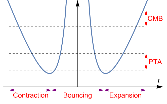
Figure 2: The evolution of Hubble horizon in bouncing cosmology.

In fact, the cross of the Hubble horizon of the primordial fluctuations is equivalent to its classicalization, which is crucial for them to be observable. Modes which never cross the Hubble horizon has a spurious divergence thus need specific treatment. As we are interested in the intepretation of recent PTA signals from PGWs originated from the contraction phase, we shall terminate our power spectrum at the scale $k_{\ast}=\mathcal{H}_{+}$, where $k_{\ast}$ refers to the upper limit of the PTA detectability. Moreover, for range of smaller $k$ (larger scales), the CMB constraint must be satisfied as well.

3.4 Junction conditions and power spectra

The remaining task is to evaluate the power spectra for the modes with $k\leq\mathcal{H}_{+}=\alpha^{2}\tau_{+}$. Here, $\alpha\tau_{+}$ should be at most of $\mathcal{O}(1)$ order, otherwise the scale factor shall change intensively in the bouncing epoch, in constrast with our short bounce assumption. Therefore, we have $\mathcal{H}_{+}\leq\alpha$, thus modes of our interest shall satisfy the condition $k<\alpha$. As a result, these modes will experience a tachyonic growth in the bouncing epoch as suggested by (3.9). In this case, the exponential growing mode will dominate over the exponential dacaying mode, so it suffices to evaluate $b_{T,1}$.

We calculate $b_{T,1}$ by applying the junction condition for tensor fluctuations, i.e., the mode function and its first derivative is continuous on the transition surface $\tau=\tau_{-}$:

$$-\frac{2^{\nu-1}i}{\sqrt{\pi}}\Gamma(\nu)k^{-\nu}\left[\frac{\alpha^{2}(1-q)\tau_{+}}{q}\right]^{\nu-\frac{1}{2}}=b_{T,1}e^{\sqrt{\alpha^{2}-k^{2}}\tau_{-}}+b_{T,2}e^{-\sqrt{\alpha^{2}-k^{2}}\tau_{-}}~{},$$ (3.10)

$$\frac{i\Gamma(\nu)2^{\nu}}{(1-2\nu)\sqrt{\pi}}k^{-\nu}\left[\frac{\alpha^{2}(1-q)\tau_{+}}{q}\right]^{\nu+\frac{1}{2}}=\sqrt{\alpha^{2}-k^{2}}\left(b_{T,1}e^{\sqrt{\alpha^{2}-k^{2}}\tau_{-}}-b_{T,2}e^{-\sqrt{\alpha^{2}-k^{2}}\tau_{-}}\right)~{}.$$ (3.11)

After some calculation one finds that it leads to

$$b_{T,1}=e^{-\sqrt{\alpha^{2}-k^{2}}\tau_{-}}\frac{2^{\nu-2}i}{\sqrt{\pi}}\Gamma(\nu)k^{-\nu}\left[\frac{q}{\alpha^{2}(1-q)\tau_{+}}\right]^{\frac{q}{1-q}}\left[\frac{\alpha^{2}(1-q)^{2}\tau_{+}}{\sqrt{\alpha^{2}-k^{2}}q^{2}}-1\right]~{},$$ (3.12)

where we apply $1-2\nu=2q/(1-q)$.

The tensor power spectrum at $\tau=\tau_{+}$ is thus

$$P_{T}=2^{-\frac{1+q}{1-q}}\frac{\Gamma^{2}(\nu)H_{+}^{2}}{\pi^{3}M_{p}^{2}a(\tau_{+})^{2}}k^{\frac{2}{1-q}}e^{2\sqrt{\alpha^{2}-k^{2}}\tau_{+}}\left[\frac{q}{\alpha^{2}(1-q)\tau_{+}}\right]^{\frac{2q}{1-q}}\left[\frac{\alpha^{2}(1-q)^{2}\tau_{+}}{\sqrt{\alpha^{2}-k^{2}}q^{2}}-1\right]^{2}~{}.$$ (3.13)

In terms of Hubble parameters:

$$P_{T}=2^{-\frac{1+q}{1-q}}\frac{\Gamma^{2}(\nu)}{\pi^{3}M_{p}^{2}}e^{\frac{2\sqrt{\alpha^{2}-k^{2}}\mathcal{H}_{+}}{\alpha^{2}}}\left(\frac{q}{1-q}\right)^{\frac{2q}{1-q}}\left(\frac{k/a_{B}}{H_{+}}\right)^{\frac{2}{1-q}}\left[\frac{(1-q)^{2}\mathcal{H}_{+}}{\sqrt{\alpha^{2}-k^{2}}q^{2}}-1\right]^{2}~{}.$$ (3.14)

We have $H_{+}=\alpha^{2}t_{+}$, since $\alpha t_{+}$ can be at most $\mathcal{O}(1)$, $H_{+}$ cannot exceed $\alpha$ too much. As a result, $\mathcal{H}_{+}\simeq a_{B}H_{+}$ must be much smaller than $\alpha$, since $a_{B}\ll a_{\rm today}$. Similarly, we have $k\leq k_{\ast}=\mathcal{H}_{+}\ll\alpha$. Thus, unless we take a vanishing $q$, the terms in bracket will approximates to unity. The expression simplifies to

$$P_{T}\simeq 2^{-\frac{1+q}{1-q}}\frac{\Gamma^{2}(\nu)}{\pi^{3}}\left(\frac{H_{+}}{M_{p}}\right)^{2}\left(\frac{q}{1-q}\right)^{\frac{2q}{1-q}}\left(\frac{k/a_{B}}{H_{+}}\right)^{\frac{2}{1-q}}~{}.$$ (3.15)

It’s easy to see that the tensor power spectrum is governed by three parameters: the Hubble parameter at the end of bouncing phase $H_{+}$, the model parameter $q$ which essentially determine the scale dependence of the primordial fluctuations, and the scale factor $a_{B}$ which is relevant to the post-bouncing phases.

From the above results we can see that, for $q\lesssim 1$, $2/(1-q)>0$, and we can get a blue-tilted tensor power spectrum. For current PTA data, it requires $n_{T}=1.8\pm 0.3$ [65], which suggests $q<0.0476$.

Moreover, in the minimal setup, the spectral energy density parameter $\Omega_{GW}(k)$ is related to the primordial tensor spectrum, defined as the energy density of the GWs per unit logarithmic frequency, by

$$\Omega_{GW}(k)\equiv\frac{1}{3H^{2}}\frac{d\rho_{\rm GW}}{d\ln k}\simeq 10^{-6}P_{T}(k)~{}.$$ (3.16)

4 Parameter Choices against Constraints

The above results shall be confronted to several theoretical and observational constraints, which can be used to confine model parameters.

First, we discuss trans-Planckian problem, i.e., the physical wavelength of primordial fluctuations we concerned here cannot be smaller than the Planck length. The power spectrum is terminated at the scale $k_{\ast}$, so the scenario is free from trans-Planckian problem if

$$\lambda_{\ast}=\frac{1}{(k_{\ast}/a_{B})}>l_{P}~{}\to~{}\frac{H_{+}}{M_{p}}<1~{},$$ (4.1)

since at $a=a_{B}$ the physical wavelength takes its minimum. Here we use the fact $k_{\ast}\simeq\mathcal{H}_{+}(\tau_{+})=a_{B}H_{+}$.

Next we are ready to confront our model with observations. As is shown in [9, 65], the tensor power spectrum at the PTA frequency range ($f=10{\rm nHz}$) is given by $P_{T}(f=10{\rm nHz})\sim 10^{-3}$. On the other hand, it is useful to define the effective e-folding number counting from $\tau_{+}$ to today:

$$N\equiv\ln\left(\frac{a_{\rm today}}{a_{B}}\right)~{},$$ (4.2)

then the tensor power spectrum (3.15) expressed by $N$ becomes

$$P_{T}(\tau_{+})\simeq 2^{-\frac{1+q}{1-q}}\frac{\Gamma^{2}(\nu)}{\pi^{3}}\left(\frac{H_{+}}{M_{p}}\right)^{2}\left(\frac{q}{1-q}\right)^{\frac{2q}{1-q}}a_{\rm today}\left(\frac{k/a_{\rm today}}{H_{+}}\right)^{\frac{2}{1-q}}e^{\frac{2}{1-q}N}~{}.$$ (4.3)

Here, we are evaluating the tensor fluctuation at $\tau_{+}$, since after that, the universe begins expansion and primordial tensor fluctuations on super-horizon scales are frozen and directly connected to observations. We also use the approximation $a(\tau_{+})\simeq a_{B}$. Connecting with observations where $a_{\rm today}=1$ and $k_{\rm PTA}/a_{\rm today}=10^{6}\rm{Mpc}^{-1}=6.6\times 10^{-33}{\rm GeV}$, the formula becomes

$$P_{T}(k_{\rm PTA},\tau_{+}) =2^{-\frac{1+q}{1-q}}\left(\frac{q}{1-q}\right)^{\frac{2q}{1-q}}\frac{\Gamma^{2}(\nu)}{\pi^{3}}e^{\frac{2}{1-q}N}$$

$$\times\left(\frac{H_{+}}{M_{p}}\right)^{2}\left(\frac{5.5\times 10^{-52}M_{p}}{H_{+}}\right)^{\frac{2}{1-q}}~{},$$ (4.4)

the value of which should be determined by model parameters.

We conclude the model parameters as well as the observables in Table. 1. Notice that, the result is insensitive to $\lambda$’s as long as $\lambda\gg 1$, as they only decide the smoothness of top-hat functions, and we choose $\lambda_{i}=20$, $i=1,2,3,4$. Also, the parameters $\phi_{-}$, $\phi_{+}$ determines the start and end of the bouncing phase. Here we’re dedicately design the value of them to let $|H_{-}|\simeq H_{+}$ to make the analytical investigation simpler . Finally, we haven’t made any assumptions on the late-time evolution of the universe, so the parameter $N$ remains free in our model. We choose the value of $N$ such that $P_{T}(10\rm{nHz})=10^{-3}$.

Model parameters							Variable	Observables
$\beta_{1}$	$\beta_{2}$	$\phi_{-}$	$\phi_{+}$	$V_{0}$	$q$	$N$	$H_{+}$	$P_{T}$(10nHz)	$n_{T}$
1.1	1	$0.0$	$2.8$	$10^{-2}$	$0.002$	115.97	$0.20$	$1.0\times 10^{-3}$	2.00
1.1	1	$-0.1$	$3.7$	$10^{-1}$	0.005	116.06	$0.22$	$1.0\times 10^{-3}$	2.01
1.1	1	$-0.1$	$2.8$	$10^{-2}$	0.01	$115.96$	$0.20$	$1.0\times 10^{-3}$	2.02
1.1	1	$0.0$	$3.6$	$10^{-3}$	0.02	116.18	$0.25$	$1.0\times 10^{-3}$	2.04

Table 1: The primordial tensor power spectrum for different model parameters. Here we normalize the parameters by setting $M_{p}=1$.

We present the resultant primordial tensor power spectrum for different model parameters in Table. 1. It’s easy to see that the PTA result can be interpreted with certain choice of model parameters. Utilizing the parameters in Table. 1, We numerically plot the results of $P_{T}$ and $\log_{10}\Omega_{GW}$ in Fig. 3. In the plot, we make comparison of the ${\Omega_{GW}}$ curves to the NANOGrav 15-year data set and find that the curves fit the data very well. Moreover one can observe that, although the paramter $q$ spans over O(10) in the sets of parameters, the curves get very closed to each other, which means that the results is not quite sensitive on the parameter $q$.

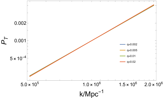
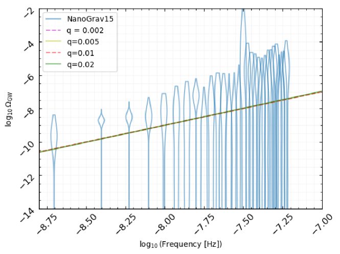
Figure 3: The tensor power spectrum and energy density spectrum for different value of $q$.

Finally, let’s determine the maximum wavenumber $k_{\ast}$ below which we’re concerning. From the above result, one can parameterize the tensor spectrum as a simpler form:

$$P_{T}(k)\simeq 10^{-3}\left(\frac{k}{10^{6}\rm{Mpc}^{-1}}\right)^{\frac{2}{1-q}}~{},$$ (4.5)

and in order to make the perturbative treatment work, one must have $P_{T}<1$ for $k\leq k_{\ast}$. This give rise to

$$\ln\left(\frac{k_{\ast}}{10^{6}{\rm Mpc}^{-1}}\right)<\frac{1-q}{2}\ln 10^{3}=3.5(1-q)~{}.$$ (4.6)

As the observed PTA data prefers $q\leq 0.0476$, the value $k_{\ast}$ can be at most of $\mathcal{O}(10^{7}){\rm Mpc}^{-1}$ order.

5 Scalar perturbations

5.1 Scalar perturbation from the Ekpyrotic field $\phi$

The dynamics for the fluctuation of the Ekpyrotic field $\phi$ is [103]

$$\mu_{k}^{\prime\prime}+\left(k^{2}-\frac{z_{s}^{\prime\prime}}{z_{s}}\right)\mu_{k}=0~{},$$ (5.1)

where $\mu_{k}\equiv z_{s}\delta\phi$ is the mode function for $\phi$ and

$$\frac{z_{s}^{2}}{a^{2}}\equiv\frac{\dot{\phi}^{2}K_{X}+\dot{\phi}^{4}K_{XX}}{H^{2}M_{p}^{2}}=\frac{3\beta_{2}\dot{\phi}^{4}+2(1-\beta_{1})M_{p}^{2}\dot{\phi}^{2}}{4M_{p}^{2}H^{2}}~{}.$$ (5.2)

As we discussed in Sec. 3.3, only the modes that becomes super-horizon in the contraction phase are of observational interest to us. For these modes, the power spectrum from $\phi$ at $\tau=\tau_{-}$ is evaluated as [103]

$$P_{\phi}(k,\tau_{-})\simeq\frac{\Gamma^{2}(\nu)(1-2\nu)^{1-2\nu}}{3\pi^{3}2^{8-4\nu}}\left(\frac{k}{|\mathcal{H}_{-}|}\right)^{\frac{2}{1-q}}\frac{H_{-}^{2}}{M_{p}^{2}}~{},~{}\nu\equiv\frac{1-3q}{2(1-q)}~{},$$ (5.3)

which is strongly blue. Correspondingly, we define the tensor-to-scalar ratio of the scalar field $\phi$, $r_{\phi}\equiv P_{T}/P_{\phi}$, therefore, at $\tau=\tau_{-}$ it is just a number $r_{\phi}=96$.

The dynamics in the bouncing phase is more involved. At first glance, the parameter $z_{s}$ diverges at the bouncing point $H=0$ according to (5.2). However, if we use (2.19), the expression for $z_{s}$ becomes

$$\frac{z_{s}^{2}}{a^{2}}=\frac{M_{p}^{2}}{4H^{2}}\frac{(1-\beta_{1})^{2}}{3\beta_{2}}\left(e^{-\frac{t^{2}}{T^{2}}}-e^{-\frac{2t^{2}}{T^{2}}}\right)~{},$$ (5.4)

which converges at the limit $t\to 0$ since $H=\alpha^{2}t$ . Moreover, at leading order we have $z_{s}/a=\rm{const}$ and thus $z_{s}^{\prime\prime}/z_{s}=a^{\prime\prime}/a$. In this case, the scalar fluctuation shares the same dynamics as the tensor fluctuation and as a result, the tensor-to-scalar ratio $r_{\phi}$ is invariant in the bouncing phase. We can thus immediately write down the power spectrum for $\phi$ at the end of bouncing phase:

$$P_{\phi}(k,\tau_{+})=P_{T}(k,\tau_{+})/r_{\phi}=\frac{1}{96}P_{T}(k,\tau_{+})~{}.$$ (5.5)

Before closing this section, we comment on the difference between our result and that in [72, 103]. The non-singular bouncing models in [72, 103] are constructed with a cubic Galileon action $\gamma G(X)\Box\phi$, in which the denominator in the expression of $z_{s}^{2}$ (5.2) become $(HM_{p}-\gamma\dot{\phi}G^{\prime}(X)/2)^{2}$. In this case, the dominant term in the denominator of (5.2) during bouncing phase is $(\gamma\dot{\phi}G^{\prime})^{2}$ instead of $H^{2}M_{p}^{2}$ in our scenario. Without the inclusion of cubic Galileon term, we simply get a constant tensor-to-scalar ratio $r_{\phi}=96$ in our model.

5.2 Scalar perturbation from curvaton field $\sigma$

As we show above, the single-field Ekpyrotic bouncing scenario predicts a blue-tilted scalar spectra, so we introduce the curvaton field $\sigma$ to get the scale-invariant power spectrum on CMB scale. The dynamical equation for the fluctuation of curvaton is

$$u_{k}^{\prime\prime}+\left(k^{2}-\frac{z_{c}^{\prime\prime}}{z_{c}}\right)u_{k}=0~{},$$ (5.6)

where $u_{k}\equiv z_{c}\delta\sigma$ is the mode function for the curvaton field and

$$z_{c}\equiv a\sqrt{\frac{M_{p}^{2}f^{2}}{\cosh(\sqrt{2/q}\phi)}}\simeq\frac{aM_{p}f}{\sqrt{e^{-\sqrt{2/q}\phi}}}=aM_{p}fe^{\frac{\phi}{\sqrt{2q}}}~{},~{}\phi\ll-1~{}.$$ (5.7)

With the help of (2.15) and (2.17), we have

$$e^{\frac{\phi}{\sqrt{2q}}}=\frac{\sqrt{q(1-3q)}}{\sqrt{2V_{0}}M_{p}t}=-\frac{\sqrt{q(1-3q)}}{\sqrt{2V_{0}}M_{p}a_{-}(1-q)}\left[\frac{(\tau_{e}-\tau)}{(\tau_{e}-\tau_{-})^{q}}\right]^{-\frac{1}{1-q}}~{}.$$ (5.8)

The background geometry (2.16) then implies

$$z_{c}=\frac{-f\sqrt{q(1-3q)}}{\sqrt{2V_{0}}(1-q)}(\tau_{e}-\tau)^{-1}~{},$$ (5.9)

so we get the following dynamical equation

$$u_{k}^{\prime\prime}+\left(k^{2}-\frac{2}{(\tau_{e}-\tau)^{2}}\right)u_{k}=0~{}.$$ (5.10)

Imposing the vacuum initial condition, the solution to (5.10) is

$$u_{k}(\tau)=\frac{\sqrt{\pi(\tau_{e}-\tau)}}{2}H_{3/2}^{(1)}[k(\tau_{e}-\tau)]=\frac{e^{ik(\tau_{e}-\tau)}}{\sqrt{2k}}\left[1+\frac{i}{k(\tau_{e}-\tau)}\right]~{},$$ (5.11)

where $H_{3/2}^{(1)}$ is the Hankel function of the first kind. For modes that become super-horizon in the contraction epoch, the corresponding power spectrum at the end of contraction phase is

$$P_{\sigma}(k,\tau_{-})=\frac{k^{3}}{2\pi^{2}}\frac{|u_{k}|^{2}}{z_{c}^{2}}\simeq\frac{V_{0}(1-q)^{2}}{2\pi^{2}f^{2}q(1-3q)a_{-}^{2}}~{}.$$ (5.12)

In the bouncing epoch, we have

$$\frac{z_{c}^{\prime\prime}}{z_{c}}\simeq\frac{a^{\prime\prime}}{a}-\frac{2}{q}\phi^{\prime 2}=\alpha^{2}(1+\alpha^{2}\tau^{2})-\frac{4(\beta_{1}-1)}{3\beta_{2}q}M_{p}^{2}e^{-\frac{2\tau^{2}}{T^{2}}-\frac{1}{2}\alpha^{2}\tau^{2}}~{},$$ (5.13)

where we’ve applied $\sinh(\sqrt{2/q}\phi)\simeq 0$ and $\sinh(\sqrt{2/q}\phi)\simeq 1$, and the formulae (2.19) is used. The dynamical equation near $\tau=0$ becomes

$$u_{k}^{\prime\prime}+\left[k^{2}-\tilde{\alpha}^{2}+\tilde{\beta}^{4}t^{2}+\mathcal{O}(t^{4})\right]u_{k}=0~{},~{}$$ (5.14)

$$\tilde{\alpha}^{2}\equiv\alpha^{2}-\frac{4(\beta_{1}-1)}{3\beta_{2}q}M_{p}^{2}~{},~{}\tilde{\beta}^{4}\equiv\alpha^{4}+\frac{4(\beta_{1}-1)}{3\beta_{2}q}M_{p}^{2}\left(\frac{2}{T^{2}}+\frac{\alpha^{2}}{2}\right)~{}.$$ (5.15)

Expanding the Friedmann’s equation (2.9) near the bouncing point gives

$$3\alpha^{4}t^{2}M_{p}^{2}\simeq\frac{(\beta_{1}-1)^{2}}{3\beta_{2}T^{2}}M_{p}^{2}t^{2}~{}\to~{}\alpha^{2}\simeq\frac{\beta_{1}-1}{3\sqrt{\beta_{2}}T}M_{p}~{}.$$ (5.16)

It’s reasonable to take the duration of bouncing phase to be much larger than a Planck time in a classical bouncing scenario. As a result $T^{-1}<M_{p}$ and we have $\tilde{\alpha}^{2}<0$ (unless $\beta_{2}$ takes an extremely small value). Therefore, the curvaton acquires an oscillatory behavior in the bouncing phase, thus its power spectrum at $\tau_{+}$ is

$$P_{\sigma}(k,\tau_{+})=P_{\sigma}(k,\tau_{-})=\frac{V_{0}(1-q)^{2}}{2\pi^{2}f^{2}q(1-3q)a_{+}^{2}}~{}.$$ (5.17)

5.3 The curvature fluctuation

The gauge-invariant curvature fluctuation usually depends on the metric perturbation and the perturbed field $\delta\phi$ and $\delta\sigma$, although the former can be ignored by taking a spatial-flat gauge. In principle, one has to work out the explicit formalism for both the field perturbations to determine $\zeta$, which is rather involving. However, in curvaton scenarios we actually don’t need to do that, since we effectively have only one field perturbation. In our case, however, which will be dominant depends on the scales we’re considering.

From the above sections we can see that, $\delta\phi$ got a blue-tilted power spectrum while $\delta\sigma$ got a scale-invariant one, so it’s natural that on small scales such as PTA scale, the dominate contribution from $P_{\zeta}$ is determined by the fluctuation of scalar field $\delta\phi$, whereas on large scales such as CMB scale, the curvature fluctuation $P_{\zeta}$ is mainly sourced from the curvaton field $\delta\sigma$.

On small scales, since both background and perturbations comes from $\phi$ field, the system effectively becomes that of a single field, and the perturbations become adiabatic. From the above sections we know that the tensor-to-scalar ratio of $\phi$ is $r_{\phi}\equiv P_{\phi}/P_{T}=96$. Moreover, as demonstrated above, the tensor power spectrum at the PTA frequency range ($f=10{\rm nHz}$) is given by $P_{T}(f=10{\rm nHz})\sim 10^{-3}$, which indicates the power spectrum of $P_{\phi}$ to be

$$P_{\phi}(k)=\frac{P_{T}}{96}\simeq 1.0\times 10^{-5}\left(\frac{k}{10^{6}{\rm Mpc}^{-1}}\right)^{\frac{2}{1-q}}~{}.$$ (5.18)

where we take the spectra index $n_{T}\equiv d\ln P_{T}/d\ln k$ to be approximately $2/(1-q)$ for illustrative purpose.

Since on small scales the perturbations becomes adiabatic, the curvature pertuurbation generated from it is simply $\zeta\simeq-(H/\dot{\phi})\delta\phi$. In the Ekpyrosis phase one has $H/\dot{\phi}=\sqrt{q/2}$, so

$$P^{(s)}_{\zeta}(k,\tau_{-})=\frac{q}{2}P_{\phi}(k,\tau_{-})~{},$$ (5.19)

where the supscript “$(s)$” denotes “small scales”. While since the bounce process is symmetric, it is reasonable to assume that $H/\dot{\phi}$ doesn’t change much after the bounce, namely $P^{(s)}_{\zeta}(k,\tau_{-})\simeq P^{(s)}_{\zeta}(k,\tau_{+})$. Moreover, in the radiation dominated epoch, both the curvature and tensor fluctuations get frozen on super-horizon scales, so

$$P^{(s)}_{\zeta}(k)\simeq P^{(s)}_{\zeta}(k,\tau_{+})\sim 10^{-5}q\left(\frac{k}{10^{6}{\rm Mpc}^{-1}}\right)^{\frac{2}{1-q}}~{},$$ (5.20)

where we’ve neglected numerical factors.

On large scales, on the other hand, the field fluctuation is solely determined by $P_{\sigma}$. However, the background is dominated by the $\phi$ field, instead of $\sigma$ field. Following the conventional treatment of curvaton mechanism, we assume that the curvaton field is converted into curvature fluctuation on its horizon re-entry event in the radiation dominated epoch, such that

$$\zeta_{k}(t_{r}(k))=-\frac{H\delta\sigma_{k}}{\dot{\sigma}}(t=t_{r}(k))~{},$$ (5.21)

where $t_{r}(k)$ labels the time of horizon re-entry event for a certain mode $k$. Since $t_{r}$ generically has $k$ dependence, a scale-invariant fluctuation of curvaton field doesn’t necessariliy lead to a a scale-invariant curvature fluctuation. To generate a nearly scale-invariant curvature fluctuation on CMB scales, we are suggested to construct the model such that $H/\dot{\sigma}={\rm const}$ in the radiation dominated epoch.

The action of curvaton field (2.8) has the schematic form $\mathcal{L}_{\sigma}=\mathcal{F}(\phi)(\partial\sigma)^{2}$, which gives the following equation of motion

$$\frac{d}{dt}\left(a^{3}\mathcal{F}(\phi)\dot{\sigma}\right)=0~{}.$$ (5.22)

Except for the trivial solution $\dot{\sigma}=0$, the evolving branch of solution is $\dot{\sigma}\propto a^{-3}\mathcal{F}(\phi)^{-1}$, and the condition becomes

$$\frac{H}{\dot{\sigma}}={\rm const}~{}\to~{}Ha^{3}\mathcal{F}(\phi)={\rm const}~{}.$$ (5.23)

In a radiation dominated universe, $a\propto t^{1/2}$, $H\propto t^{-1}$ and $\dot{\phi}\propto\sqrt{H}=t^{-1/2}$ from the Friedmann’s equation $H^{2}\propto X^{2}$. We then have $\phi\propto t^{1/2}$ and taking $\mathcal{F}(\phi)\propto\phi^{-1}$ could meet the condition (5.23). This justifies the choice of curvation action (2.8).

Since now $H/\dot{\sigma}$ is a constant with no time dependence, we define $s\equiv H/\dot{\sigma}|_{\tau=\tau_{+}}$ which is determined by the initial values of $H$ and $\dot{\sigma}$ in the radiation dominated epoch. This gives

$$P^{(l)}_{\zeta}(k)=s^{2}P_{\sigma}=\frac{s^{2}V_{0}(1-q)^{2}}{2\pi^{2}f^{2}q(1-3q)a_{+}^{2}}~{},$$ (5.24)

where the supscript “$(l)$” denotes “large scales”. Moreover, when we compare this result to the CMB constraint, we have

$$P^{(l)}_{\zeta}(k_{\rm CMB})=\frac{s^{2}V_{0}(1-q)^{2}}{2\pi^{2}f^{2}q(1-3q)a_{+}^{2}}\simeq 2.1\times 10^{-9}~{}.$$ (5.25)

and is scale-invariant till the re-entry of the horizon.

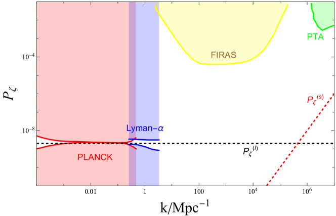
Figure 4: The power spectrum of $P^{s}_{\zeta}$ and $P^{l}_{\zeta}$, denoted by the red and black dashed lines respectively. The shaded region represents the constraint for the power spectrum of curvature perturbation $P_{\zeta}$ from Planck [123], Lyman-$\alpha$ [124], FIRAS [125, 126] (see also [127, 128]) and PTA [129]. Here we take $q=0.001$.

We depict the power spectrum of $P^{(s)}_{\zeta}$, $P^{(l)}_{\zeta}$ in Fig. 4. It’s easy to see that on the CMB scale, the curvature fluctuation $P_{\zeta}$ is mainly sourced from the curvaton field, whereas on the PTA range, the dominate contribution from $P_{\zeta}$ is determined by the fluctuation of scalar field $\delta\phi$. Moreover, taking $q=0.05$ as is allowed by PTA data, one can obtain the pivot scale where the perturbation of $\phi$ exceeds that of $\sigma$ by equaling Eqs. (5.20) and (5.25). This will give rise to the result:

$$k_{\rm pivot}\simeq 10^{-5}{\rm Mpc}^{-1}~{}.$$ (5.26)

6 Conclusion and Outlook

The recently released PTA data of GW indicates that, if the GW is to be interpreted as from primordial tensor perturbation, then the tensor spectrum should be strongly blue-tilted. On the other hand, it is well-known that the Ekpyrosis-bounce scenario can provide tensor spectrum with spectral index $2<n_{T}<3$. So there is large possibility that such tensor perturbation may originate from the Ekpyrosis-bounce cosmology.

To illustrate this, in this paper we improve the study in [81] and present a concrete realization. Since the contracting phase preceding the bounce is Ekpyrotic-like where the EoS is much larger than unity, the anisotropic problem can be naturally removed. Moreover, although not much discussed in the current work, it is not difficult to understand that the ghost problem can also be alliminate by taking into account certain corrections, e.g., from Galileon theories. Bounce process are realized with numerical calculations, and finally, after the bounce, the universe safely evolves into a radiation-dominant phase, connecting with standard Big Bang cosmology.

The calculation of tensor perturbations is somehow straightforward. The tensor perturbations exit the horizon during the ekpyrotic phase, so their spectrum is blue-tilted. This feature can be inherited in radiation dominate phase, till the re-entry of the horizon in expanding phase. We have shown that after appropriately choosing model parameters, one can fit the PTA data very well. Moreover, we consider the constraints of the parameters against various constraints. The model is free of Trans-Planckian problem by requiring $H_{+}<M_{p}$. Moreover, considering the perturbation theory not being ruined, the bounce scenario can account for primordial GWs with wave number up to $10^{7}{\rm Mpc}^{-1}$, containing the range of PTA detection.

However, it is well known that the Ekpyrotic scenario also gives rise to blue spectrum to scalar perturbation, which conflicts with the CMB observations. In order to cure this problem, it is helpful to introduce a curvaton field $\sigma$, which couples to the Ekpyrotic field $\phi$. Due to the nontrivial coupling, the curvaton field can generate scale-invariant scalar perturbations, which will transfer to curvature perturbations after curvaton decay. We delicately design the form of coupling which can realize scale-invariance, and we also checked that the backreaction will not ruin the Ekpyrotic-bouncing background. Moreover, the blue-tilted perturbation of Ekpyrotic field will be suppressed on CMB scales, while be dominant on PTA scales. However, since it is still small compared to tensor perturbations with tiny tensor-to-scalar ratio, the problem of an oversized scalar fluctuation appeared in [81] is also solved in our improved model.

A couple of future works are in order. First of all, we see that the scalar perturbation becomes dominant in small scales, which might have contributions on the matter power spectrum, and affect the consequent late-time evolution of perturbations and galaxy/large scale structure formation. Moreover, it seems that the current scalar perturbations are still not sufficient to generate Primordial Black Holes (PBHs), therefore it is also interesting to investigate how the PBHs can be generated from our scenario (see e.g., [130, 131] for studies of PBH formation in bouncing cosmology, and see [132] for other recent considerations). We will postpone this studies in a upcoming paper.

References

- [1] M. Novello and S. E. P. Bergliaffa, “Bouncing Cosmologies,” Phys. Rept. 463 (2008) 127–213, arXiv:0802.1634 [astro-ph].
- [2] A. Borde and A. Vilenkin, “Eternal inflation and the initial singularity,” Phys. Rev. Lett. 72 (1994) 3305–3309, arXiv:gr-qc/9312022.
- [3] A. Borde, A. H. Guth, and A. Vilenkin, “Inflationary space-times are incompletein past directions,” Phys. Rev. Lett. 90 (2003) 151301, arXiv:gr-qc/0110012.
- [4] J. E. Lesnefsky, D. A. Easson, and P. C. W. Davies, “Past-completeness of inflationary spacetimes,” Phys. Rev. D 107 no. 4, (2023) 044024, arXiv:2207.00955 [gr-qc].
- [5] G. Geshnizjani, E. Ling, and J. Quintin, “On the initial singularity and extendibility of flat quasi-de Sitter spacetimes,” arXiv:2305.01676 [gr-qc].
- [6] R. H. Brandenberger and J. Martin, “The Robustness of inflation to changes in superPlanck scale physics,” Mod. Phys. Lett. A 16 (2001) 999–1006, arXiv:astro-ph/0005432.
- [7] J. Martin and R. H. Brandenberger, “The TransPlanckian problem of inflationary cosmology,” Phys. Rev. D 63 (2001) 123501, arXiv:hep-th/0005209.
- [8] A. Ijjas and P. J. Steinhardt, “Bouncing Cosmology made simple,” Class. Quant. Grav. 35 no. 13, (2018) 135004, arXiv:1803.01961 [astro-ph.CO].
- [9] NANOGrav Collaboration, A. Afzal et al., “The NANOGrav 15 yr Data Set: Search for Signals from New Physics,” Astrophys. J. Lett. 951 no. 1, (2023) L11, arXiv:2306.16219 [astro-ph.HE].
- [10] NANOGrav Collaboration, G. Agazie et al., “The NANOGrav 15 yr Data Set: Evidence for a Gravitational-wave Background,” Astrophys. J. Lett. 951 no. 1, (2023) L8, arXiv:2306.16213 [astro-ph.HE].
- [11] J. Antoniadis et al., “The second data release from the European Pulsar Timing Array III. Search for gravitational wave signals,” arXiv:2306.16214 [astro-ph.HE].
- [12] D. J. Reardon et al., “Search for an Isotropic Gravitational-wave Background with the Parkes Pulsar Timing Array,” Astrophys. J. Lett. 951 no. 1, (2023) L6, arXiv:2306.16215 [astro-ph.HE].
- [13] H. Xu et al., “Searching for the Nano-Hertz Stochastic Gravitational Wave Background with the Chinese Pulsar Timing Array Data Release I,” Res. Astron. Astrophys. 23 no. 7, (2023) 075024, arXiv:2306.16216 [astro-ph.HE].
- [14] E. Battista and V. De Falco, “First post-Newtonian generation of gravitational waves in Einstein-Cartan theory,” Phys. Rev. D 104 no. 8, (2021) 084067, arXiv:2109.01384 [gr-qc].
- [15] E. Battista and V. De Falco, “Gravitational waves at the first post-Newtonian order with the Weyssenhoff fluid in Einstein–Cartan theory,” Eur. Phys. J. C 82 no. 7, (2022) 628, arXiv:2206.12907 [gr-qc].
- [16] A. Ashoorioon, K. Rezazadeh, and A. Rostami, “NANOGrav signal from the end of inflation and the LIGO mass and heavier primordial black holes,” Phys. Lett. B 835 (2022) 137542, arXiv:2202.01131 [astro-ph.CO].
- [17] J. Ellis, M. Lewicki, C. Lin, and V. Vaskonen, “Cosmic superstrings revisited in light of NANOGrav 15-year data,” Phys. Rev. D 108 no. 10, (2023) 103511, arXiv:2306.17147 [astro-ph.CO].
- [18] J. Ellis, M. Fairbairn, G. Hütsi, J. Raidal, J. Urrutia, V. Vaskonen, and H. Veermäe, “Gravitational waves from supermassive black hole binaries in light of the NANOGrav 15-year data,” Phys. Rev. D 109 no. 2, (2024) L021302, arXiv:2306.17021 [astro-ph.CO].
- [19] G. Franciolini, A. Iovino, Junior., V. Vaskonen, and H. Veermae, “Recent Gravitational Wave Observation by Pulsar Timing Arrays and Primordial Black Holes: The Importance of Non-Gaussianities,” Phys. Rev. Lett. 131 no. 20, (2023) 201401, arXiv:2306.17149 [astro-ph.CO].
- [20] C. Zhang, N. Dai, Q. Gao, Y. Gong, T. Jiang, and X. Lu, “Detecting new fundamental fields with pulsar timing arrays,” Phys. Rev. D 108 no. 10, (2023) 104069, arXiv:2307.01093 [gr-qc].
- [21] E. Cannizzaro, G. Franciolini, and P. Pani, “Novel tests of gravity using nano-Hertz stochastic gravitational-wave background signals,” JCAP 04 (2024) 056, arXiv:2307.11665 [gr-qc].
- [22] Z.-Q. Shen, G.-W. Yuan, Y.-Y. Wang, and Y.-Z. Wang, “Dark Matter Spike surrounding Supermassive Black Holes Binary and the nanohertz Stochastic Gravitational Wave Background,” arXiv:2306.17143 [astro-ph.HE].
- [23] X. K. Du, M. X. Huang, F. Wang, and Y. K. Zhang, “Did the nHZ Gravitational Waves Signatures Observed By NANOGrav Indicate Multiple Sector SUSY Breaking?,” arXiv:2307.02938 [hep-ph].
- [24] S. Balaji, G. Domènech, and G. Franciolini, “Scalar-induced gravitational wave interpretation of PTA data: the role of scalar fluctuation propagation speed,” JCAP 10 (2023) 041, arXiv:2307.08552 [gr-qc].
- [25] Z. Zhang, C. Cai, Y.-H. Su, S. Wang, Z.-H. Yu, and H.-H. Zhang, “Nano-Hertz gravitational waves from collapsing domain walls associated with freeze-in dark matter in light of pulsar timing array observations,” Phys. Rev. D 108 no. 9, (2023) 095037, arXiv:2307.11495 [hep-ph].
- [26] R. A. Konoplya and A. Zhidenko, “Asymptotic tails of massive gravitons in light of pulsar timing array observations,” Phys. Lett. B 853 (2024) 138685, arXiv:2307.01110 [gr-qc].
- [27] Y.-M. Wu, Z.-C. Chen, and Q.-G. Huang, “Cosmological interpretation for the stochastic signal in pulsar timing arrays,” Sci. China Phys. Mech. Astron. 67 no. 4, (2024) 240412, arXiv:2307.03141 [astro-ph.CO].
- [28] T. Ghosh, A. Ghoshal, H.-K. Guo, F. Hajkarim, S. F. King, K. Sinha, X. Wang, and G. White, “Did we hear the sound of the Universe boiling? Analysis using the full fluid velocity profiles and NANOGrav 15-year data,” JCAP 05 (2024) 100, arXiv:2307.02259 [astro-ph.HE].
- [29] H.-L. Huang, Y. Cai, J.-Q. Jiang, J. Zhang, and Y.-S. Piao, “Supermassive primordial black holes in multiverse: for nano-Hertz gravitational wave and high-redshift JWST galaxies,” arXiv:2306.17577 [gr-qc].
- [30] L. Liu, Z.-C. Chen, and Q.-G. Huang, “Probing the equation of state of the early Universe with pulsar timing arrays,” JCAP 11 (2023) 071, arXiv:2307.14911 [astro-ph.CO].
- [31] Y.-F. Cai, X.-C. He, X.-H. Ma, S.-F. Yan, and G.-W. Yuan, “Limits on scalar-induced gravitational waves from the stochastic background by pulsar timing array observations,” Sci. Bull. 68 (2023) 2929–2935, arXiv:2306.17822 [gr-qc].
- [32] L. Liu, Z.-C. Chen, and Q.-G. Huang, “Implications for the non-Gaussianity of curvature perturbation from pulsar timing arrays,” Phys. Rev. D 109 no. 6, (2024) L061301, arXiv:2307.01102 [astro-ph.CO].
- [33] S. Jiang, A. Yang, J. Ma, and F. P. Huang, “Implication of nano-Hertz stochastic gravitational wave on dynamical dark matter through a dark first-order phase transition,” Class. Quant. Grav. 41 no. 6, (2024) 065009, arXiv:2306.17827 [hep-ph].
- [34] Y. Cai, M. Zhu, and Y.-S. Piao, “Primordial Black Holes from Null Energy Condition Violation during Inflation,” Phys. Rev. Lett. 133 no. 2, (2024) 021001, arXiv:2305.10933 [gr-qc].
- [35] R. Maji and W.-I. Park, “Supersymmetric U(1)B-L flat direction and NANOGrav 15 year data,” JCAP 01 (2024) 015, arXiv:2308.11439 [hep-ph].
- [36] A. Addazi, Y.-F. Cai, A. Marciano, and L. Visinelli, “Have pulsar timing array methods detected a cosmological phase transition?,” Phys. Rev. D 109 no. 1, (2024) 015028, arXiv:2306.17205 [astro-ph.CO].
- [37] J. Ellis, M. Fairbairn, G. Franciolini, G. Hütsi, A. Iovino, M. Lewicki, M. Raidal, J. Urrutia, V. Vaskonen, and H. Veermäe, “What is the source of the PTA GW signal?,” Phys. Rev. D 109 no. 2, (2024) 023522, arXiv:2308.08546 [astro-ph.CO].
- [38] S.-P. Li and K.-P. Xie, “Collider test of nano-Hertz gravitational waves from pulsar timing arrays,” Phys. Rev. D 108 no. 5, (2023) 055018, arXiv:2307.01086 [hep-ph].
- [39] Y. Xiao, J. M. Yang, and Y. Zhang, “Implications of nano-Hertz gravitational waves on electroweak phase transition in the singlet dark matter model,” Sci. Bull. 68 (2023) 3158–3164, arXiv:2307.01072 [hep-ph].
- [40] C. Han, K.-P. Xie, J. M. Yang, and M. Zhang, “Self-interacting dark matter implied by nano-Hertz gravitational waves,” Phys. Rev. D 109 no. 11, (2024) 115025, arXiv:2306.16966 [hep-ph].
- [41] V. K. Oikonomou, “Effects of the axion through the Higgs portal on primordial gravitational waves during the electroweak breaking,” Phys. Rev. D 107 no. 6, (2023) 064071, arXiv:2303.05889 [hep-ph].
- [42] L. Bian, S. Ge, J. Shu, B. Wang, X.-Y. Yang, and J. Zong, “Gravitational wave sources for pulsar timing arrays,” Phys. Rev. D 109 no. 10, (2024) L101301, arXiv:2307.02376 [astro-ph.HE].
- [43] M. X. Huang, F. Wang, and Y. K. Zhang, “Interplay between the muon g-2 anomaly and the PTA nHZ gravitational waves from domain walls in the next-to-minimal supersymmetric standard model,” Phys. Rev. D 109 no. 7, (2024) 075032, arXiv:2309.06378 [hep-ph].
- [44] G. Ye and A. Silvestri, “Can the Gravitational Wave Background Feel Wiggles in Spacetime?,” Astrophys. J. Lett. 963 no. 1, (2024) L15, arXiv:2307.05455 [astro-ph.CO].
- [45] S.-Y. Guo, M. Khlopov, X. Liu, L. Wu, Y. Wu, and B. Zhu, “Footprints of Axion-Like Particle in Pulsar Timing Array Data and JWST Observations,” arXiv:2306.17022 [hep-ph].
- [46] S. Choudhury, “Single field inflation in the light of Pulsar Timing Array Data: quintessential interpretation of blue tilted tensor spectrum through Non-Bunch Davies initial condition,” Eur. Phys. J. C 84 no. 3, (2024) 278, arXiv:2307.03249 [astro-ph.CO].
- [47] J.-Q. Jiang, Y. Cai, G. Ye, and Y.-S. Piao, “Broken blue-tilted inflationary gravitational waves: a joint analysis of NANOGrav 15-year and BICEP/Keck 2018 data,” JCAP 05 (2024) 004, arXiv:2307.15547 [astro-ph.CO].
- [48] V. K. Oikonomou, “A Stiff Pre-CMB Era with a Mildly Blue-tilted Tensor Inflationary Era can Explain the 2023 NANOGrav Signal,” arXiv:2309.04850 [astro-ph.CO].
- [49] S. Choudhury, K. Dey, A. Karde, S. Panda, and M. Sami, “Primordial non-Gaussianity as a saviour for PBH overproduction in SIGWs generated by pulsar timing arrays for Galileon inflation,” Phys. Lett. B 856 (2024) 138925, arXiv:2310.11034 [astro-ph.CO].
- [50] K. D. Lozanov, S. Pi, M. Sasaki, V. Takhistov, and A. Wang, “Axion Universal Gravitational Wave Interpretation of Pulsar Timing Array Data,” arXiv:2310.03594 [astro-ph.CO].
- [51] V. K. Oikonomou, “Flat energy spectrum of primordial gravitational waves versus peaks and the NANOGrav 2023 observation,” Phys. Rev. D 108 no. 4, (2023) 043516, arXiv:2306.17351 [astro-ph.CO].
- [52] S. Choudhury, K. Dey, and A. Karde, “Untangling PBH overproduction in -SIGWs generated by Pulsar Timing Arrays for MST-EFT of single field inflation,” arXiv:2311.15065 [astro-ph.CO].
- [53] L. Liu, Y. Wu, and Z.-C. Chen, “Simultaneously probing the sound speed and equation of state of the early Universe with pulsar timing arrays,” JCAP 04 (2024) 011, arXiv:2310.16500 [astro-ph.CO].
- [54] G. Ye, M. Zhu, and Y. Cai, “Null energy condition violation during inflation and pulsar timing array observations,” JHEP 02 (2024) 008, arXiv:2312.10685 [gr-qc].
- [55] D. Chowdhury, A. Hait, S. Mohanty, and S. Prakash, “Ultralight vector dark matter interpretation of NANOGrav observations,” arXiv:2311.10148 [hep-ph].
- [56] Z.-C. Chen, J. Li, L. Liu, and Z. Yi, “Probing the speed of scalar-induced gravitational waves with pulsar timing arrays,” Phys. Rev. D 109 no. 10, (2024) L101302, arXiv:2401.09818 [gr-qc].
- [57] J.-Q. Jiang and Y.-S. Piao, “Search for the non-linearities of gravitational wave background in NANOGrav 15-year data set,” arXiv:2401.16950 [gr-qc].
- [58] Z.-C. Chen and L. Liu, “Can we distinguish the adiabatic fluctuations and isocurvature fluctuations with pulsar timing arrays?,” arXiv:2402.16781 [astro-ph.CO].
- [59] S. Choudhury, S. Ganguly, S. Panda, S. SenGupta, and P. Tiwari, “Obviating PBH overproduction for SIGWs generated by Pulsar Timing Arrays in loop corrected EFT of bounce,” arXiv:2407.18976 [astro-ph.CO].
- [60] Z.-C. Chen and L. Liu, “Constraints on inflation with null energy condition violation from advanced LIGO and advanced Virgo’s first three observing runs,” JCAP 06 (2024) 028, arXiv:2404.07075 [gr-qc].
- [61] C. Li, “Primordial Gravitational Waves of Big Bounce Cosmology in Light of Stochastic Gravitational Wave Background,” arXiv:2407.10071 [astro-ph.CO].
- [62] Z.-C. Chen and L. Liu, “Detecting a Gravitational-Wave Background from Null Energy Condition Violation: Prospects for Taiji,” arXiv:2404.08375 [gr-qc].
- [63] C. Pallis, “PeV-Scale SUSY and Cosmic Strings from F-Term Hybrid Inflation,” Universe 10 no. 5, (2024) , arXiv:2403.09385 [hep-ph].
- [64] C. Li, J. Lai, J. Xiang, and C. Wu, “Dual Inflation and Bounce Cosmologies Interpretation of Pulsar Timing Array Data,” arXiv:2405.15889 [astro-ph.CO].
- [65] S. Vagnozzi, “Inflationary interpretation of the stochastic gravitational wave background signal detected by pulsar timing array experiments,” JHEAp 39 (2023) 81–98, arXiv:2306.16912 [astro-ph.CO].
- [66] Y. Wang and W. Xue, “Inflation and Alternatives with Blue Tensor Spectra,” JCAP 10 (2014) 075, arXiv:1403.5817 [astro-ph.CO].
- [67] J. Khoury, B. A. Ovrut, P. J. Steinhardt, and N. Turok, “The Ekpyrotic universe: Colliding branes and the origin of the hot big bang,” Phys. Rev. D 64 (2001) 123522, arXiv:hep-th/0103239.
- [68] R. H. Brandenberger, “Alternatives to the inflationary paradigm of structure formation,” Int. J. Mod. Phys. Conf. Ser. 01 (2011) 67–79, arXiv:0902.4731 [hep-th].
- [69] R. Brandenberger and Z. Wang, “Nonsingular Ekpyrotic Cosmology with a Nearly Scale-Invariant Spectrum of Cosmological Perturbations and Gravitational Waves,” Phys. Rev. D 101 no. 6, (2020) 063522, arXiv:2001.00638 [hep-th].
- [70] T. Qiu, J. Evslin, Y.-F. Cai, M. Li, and X. Zhang, “Bouncing Galileon Cosmologies,” JCAP 10 (2011) 036, arXiv:1108.0593 [hep-th].
- [71] Y.-F. Cai, C. Gao, and E. N. Saridakis, “Bounce and cyclic cosmology in extended nonlinear massive gravity,” JCAP 10 (2012) 048, arXiv:1207.3786 [astro-ph.CO].
- [72] Y.-F. Cai, D. A. Easson, and R. Brandenberger, “Towards a Nonsingular Bouncing Cosmology,” JCAP 08 (2012) 020, arXiv:1206.2382 [hep-th].
- [73] Y.-F. Cai and E. Wilson-Ewing, “A CDM bounce scenario,” JCAP 03 (2015) 006, arXiv:1412.2914 [gr-qc].
- [74] T. Qiu and Y.-T. Wang, “G-Bounce Inflation: Towards Nonsingular Inflation Cosmology with Galileon Field,” JHEP 04 (2015) 130, arXiv:1501.03568 [astro-ph.CO].
- [75] Y. Wan, T. Qiu, F. P. Huang, Y.-F. Cai, H. Li, and X. Zhang, “Bounce Inflation Cosmology with Standard Model Higgs Boson,” JCAP 12 (2015) 019, arXiv:1509.08772 [gr-qc].
- [76] H.-G. Li, Y. Cai, and Y.-S. Piao, “Towards the bounce inflationary gravitational wave,” Eur. Phys. J. C 76 no. 12, (2016) 699, arXiv:1605.09586 [gr-qc].
- [77] Y.-F. Cai, A. Marciano, D.-G. Wang, and E. Wilson-Ewing, “Bouncing cosmologies with dark matter and dark energy,” Universe 3 no. 1, (2016) 1, arXiv:1610.00938 [astro-ph.CO].
- [78] Y. Cai, Y.-T. Wang, J.-Y. Zhao, and Y.-S. Piao, “Primordial perturbations with pre-inflationary bounce,” Phys. Rev. D 97 no. 10, (2018) 103535, arXiv:1709.07464 [astro-ph.CO].
- [79] T. Qiu, K. Tian, and S. Bu, “Perturbations of bounce inflation scenario from modified gravity revisited,” Eur. Phys. J. C 79 no. 3, (2019) 261, arXiv:1810.04436 [gr-qc].
- [80] K. Hu, T. Paul, and T. Qiu, “Tensor perturbations from bounce inflation scenario in f(Q) gravity,” Sci. China Phys. Mech. Astron. 67 no. 2, (2024) 220413, arXiv:2308.00647 [hep-th].
- [81] M. Zhu, G. Ye, and Y. Cai, “Pulsar timing array observations as a possible hint for nonsingular cosmology,” arXiv:2307.16211 [astro-ph.CO].
- [82] A. Ijjas, W. G. Cook, F. Pretorius, P. J. Steinhardt, and E. Y. Davies, “Robustness of slow contraction to cosmic initial conditions,” JCAP 08 (2020) 030, arXiv:2006.04999 [gr-qc].
- [83] T. Qiu, X. Gao, and E. N. Saridakis, “Towards anisotropy-free and nonsingular bounce cosmology with scale-invariant perturbations,” Phys. Rev. D 88 no. 4, (2013) 043525, arXiv:1303.2372 [astro-ph.CO].
- [84] N. Arkani-Hamed, H.-C. Cheng, M. A. Luty, and S. Mukohyama, “Ghost condensation and a consistent infrared modification of gravity,” JHEP 05 (2004) 074, arXiv:hep-th/0312099.
- [85] M. Libanov, S. Mironov, and V. Rubakov, “Generalized Galileons: instabilities of bouncing and Genesis cosmologies and modified Genesis,” JCAP 08 (2016) 037, arXiv:1605.05992 [hep-th].
- [86] T. Kobayashi, “Generic instabilities of nonsingular cosmologies in Horndeski theory: A no-go theorem,” Phys. Rev. D 94 no. 4, (2016) 043511, arXiv:1606.05831 [hep-th].
- [87] S. Akama and T. Kobayashi, “Generalized multi-Galileons, covariantized new terms, and the no-go theorem for nonsingular cosmologies,” Phys. Rev. D 95 no. 6, (2017) 064011, arXiv:1701.02926 [hep-th].
- [88] Y. Cai, Y. Wan, H.-G. Li, T. Qiu, and Y.-S. Piao, “The Effective Field Theory of nonsingular cosmology,” JHEP 01 (2017) 090, arXiv:1610.03400 [gr-qc].
- [89] Y. Cai, H.-G. Li, T. Qiu, and Y.-S. Piao, “The Effective Field Theory of nonsingular cosmology: II,” Eur. Phys. J. C 77 no. 6, (2017) 369, arXiv:1701.04330 [gr-qc].
- [90] Y. Cai and Y.-S. Piao, “A covariant Lagrangian for stable nonsingular bounce,” JHEP 09 (2017) 027, arXiv:1705.03401 [gr-qc].
- [91] C. Li, Y. Cai, Y.-F. Cai, and E. N. Saridakis, “The effective field theory approach of teleparallel gravity, gravity and beyond,” JCAP 10 (2018) 001, arXiv:1803.09818 [gr-qc].
- [92] R. Kolevatov, S. Mironov, N. Sukhov, and V. Volkova, “Cosmological bounce and Genesis beyond Horndeski,” JCAP 08 (2017) 038, arXiv:1705.06626 [hep-th].
- [93] S. Mironov, V. Rubakov, and V. Volkova, “Bounce beyond Horndeski with GR asymptotics and -crossing,” JCAP 10 (2018) 050, arXiv:1807.08361 [hep-th].
- [94] S. S. Boruah, H. J. Kim, M. Rouben, and G. Geshnizjani, “Cuscuton bounce,” JCAP 08 (2018) 031, arXiv:1802.06818 [gr-qc].
- [95] S. Banerjee, Y.-F. Cai, and E. N. Saridakis, “Evading the theoretical no-go theorem for nonsingular bounces in Horndeski/Galileon cosmology,” Class. Quant. Grav. 36 no. 13, (2019) 135009, arXiv:1808.01170 [gr-qc].
- [96] V. E. Volkova, S. A. Mironov, and V. A. Rubakov, “Cosmological Scenarios with Bounce and Genesis in Horndeski Theory and Beyond,” J. Exp. Theor. Phys. 129 no. 4, (2019) 553–565.
- [97] S. Mironov and A. Shtennikova, “Stable cosmological solutions in Horndeski theory,” JCAP 06 (2023) 037, arXiv:2212.03285 [gr-qc].
- [98] S. Mironov and V. Volkova, “Stable nonsingular cosmologies in beyond Horndeski theory and disformal transformations,” Int. J. Mod. Phys. A 37 no. 14, (2022) 2250088, arXiv:2204.05889 [hep-th].
- [99] A. Ganz, P. Martens, S. Mukohyama, and R. Namba, “Bouncing cosmology in VCDM,” JCAP 04 (2023) 060, arXiv:2212.13561 [gr-qc].
- [100] A. Ilyas, M. Zhu, Y. Zheng, Y.-F. Cai, and E. N. Saridakis, “DHOST Bounce,” JCAP 09 (2020) 002, arXiv:2002.08269 [gr-qc].
- [101] A. Ilyas, M. Zhu, Y. Zheng, and Y.-F. Cai, “Emergent Universe and Genesis from the DHOST Cosmology,” JHEP 01 (2021) 141, arXiv:2009.10351 [gr-qc].
- [102] M. Zhu and Y. Zheng, “Improved DHOST Genesis,” JHEP 11 (2021) 163, arXiv:2109.05277 [gr-qc].
- [103] M. Zhu, A. Ilyas, Y. Zheng, Y.-F. Cai, and E. N. Saridakis, “Scalar and tensor perturbations in DHOST bounce cosmology,” JCAP 11 no. 11, (2021) 045, arXiv:2108.01339 [gr-qc].
- [104] P. Creminelli, A. Nicolis, and M. Zaldarriaga, “Perturbations in bouncing cosmologies: Dynamical attractor versus scale invariance,” Phys. Rev. D 71 (2005) 063505, arXiv:hep-th/0411270.
- [105] Y.-S. Piao and Y.-Z. Zhang, “The Primordial perturbation spectrum from various expanding and contracting phases,” Phys. Rev. D 70 (2004) 043516, arXiv:astro-ph/0403671.
- [106] Y.-S. Piao, “On the dualities of primordial perturbation spectrums,” Phys. Lett. B 606 (2005) 245–250, arXiv:hep-th/0404002.
- [107] T. Qiu, “Reconstruction of a Nonminimal Coupling Theory with Scale-invariant Power Spectrum,” JCAP 06 (2012) 041, arXiv:1204.0189 [hep-ph].
- [108] T. Qiu, “Reconstruction of f(R) models with Scale-invariant Power Spectrum,” Phys. Lett. B 718 (2012) 475–481, arXiv:1208.4759 [astro-ph.CO].
- [109] J. Shi, Z. Fang, and T. Qiu, “Adiabatic duality: Duality of cosmological models with varying slow-roll parameter and sound speed,” Phys. Rev. D 104 no. 6, (2021) 063520, arXiv:2103.11634 [gr-qc].
- [110] D. H. Lyth and D. Wands, “Generating the curvature perturbation without an inflaton,” Phys. Lett. B 524 (2002) 5–14, arXiv:hep-ph/0110002.
- [111] D. H. Lyth, C. Ungarelli, and D. Wands, “The Primordial density perturbation in the curvaton scenario,” Phys. Rev. D 67 (2003) 023503, arXiv:astro-ph/0208055.
- [112] M. Libanov, S. Mironov, and V. Rubakov, “Non-Gaussianity of scalar perturbations generated by conformal mechanisms,” Phys. Rev. D 84 (2011) 083502, arXiv:1105.6230 [astro-ph.CO].
- [113] K. Hinterbichler and J. Khoury, “The Pseudo-Conformal Universe: Scale Invariance from Spontaneous Breaking of Conformal Symmetry,” JCAP 04 (2012) 023, arXiv:1106.1428 [hep-th].
- [114] P. Creminelli, “Conformal invariance of scalar perturbations in inflation,” Phys. Rev. D 85 (2012) 041302, arXiv:1108.0874 [hep-th].
- [115] H. Wang, T. Qiu, and Y.-S. Piao, “G-Curvaton,” Phys. Lett. B 707 (2012) 11–21, arXiv:1110.1795 [hep-ph].
- [116] K. Feng, T. Qiu, and Y.-S. Piao, “Curvaton with nonminimal derivative coupling to gravity,” Phys. Lett. B 729 (2014) 99–107, arXiv:1307.7864 [hep-th].
- [117] K. Feng and T. Qiu, “Curvaton with nonminimal derivative coupling to gravity: Full perturbation analysis,” Phys. Rev. D 90 no. 12, (2014) 123508, arXiv:1409.2949 [hep-th].
- [118] T. Qiu and K. Feng, “Reheating mechanism of the curvaton with nonminimal derivative coupling to gravity,” Eur. Phys. J. C 77 no. 10, (2017) 687, arXiv:1608.01752 [hep-ph].
- [119] X.-z. Zhang, L.-h. Liu, and T. Qiu, “Mimetic curvaton,” Phys. Rev. D 107 no. 4, (2023) 043510, arXiv:2207.07873 [hep-th].
- [120] A. Xiong, X.-z. Zhang, and T. Qiu, “Perturbations of Mimetic Curvaton,” arXiv:2405.06921 [gr-qc].
- [121] B. Xue and P. J. Steinhardt, “Evolution of curvature and anisotropy near a nonsingular bounce,” Phys. Rev. D 84 (2011) 083520, arXiv:1106.1416 [hep-th].
- [122] D. A. Easson, I. Sawicki, and A. Vikman, “G-Bounce,” JCAP 11 (2011) 021, arXiv:1109.1047 [hep-th].
- [123] Planck Collaboration, Y. Akrami et al., “Planck 2018 results. X. Constraints on inflation,” Astron. Astrophys. 641 (2020) A10, arXiv:1807.06211 [astro-ph.CO].
- [124] S. Bird, H. V. Peiris, M. Viel, and L. Verde, “Minimally Parametric Power Spectrum Reconstruction from the Lyman-alpha Forest,” Mon. Not. Roy. Astron. Soc. 413 (2011) 1717–1728, arXiv:1010.1519 [astro-ph.CO].
- [125] D. J. Fixsen, E. S. Cheng, J. M. Gales, J. C. Mather, R. A. Shafer, and E. L. Wright, “The Cosmic Microwave Background spectrum from the full COBE FIRAS data set,” Astrophys. J. 473 (1996) 576, arXiv:astro-ph/9605054.
- [126] J. Chluba, A. L. Erickcek, and I. Ben-Dayan, “Probing the inflaton: Small-scale power spectrum constraints from measurements of the CMB energy spectrum,” Astrophys. J. 758 (2012) 76, arXiv:1203.2681 [astro-ph.CO].
- [127] J. Chluba, R. Khatri, and R. A. Sunyaev, “CMB at 2x2 order: The dissipation of primordial acoustic waves and the observable part of the associated energy release,” Mon. Not. Roy. Astron. Soc. 425 (2012) 1129–1169, arXiv:1202.0057 [astro-ph.CO].
- [128] B. Cyr, T. Kite, J. Chluba, J. C. Hill, D. Jeong, S. K. Acharya, B. Bolliet, and S. P. Patil, “Disentangling the primordial nature of stochastic gravitational wave backgrounds with CMB spectral distortions,” Mon. Not. Roy. Astron. Soc. 528 no. 1, (2024) 883–897, arXiv:2309.02366 [astro-ph.CO].
- [129] C. T. Byrnes, P. S. Cole, and S. P. Patil, “Steepest growth of the power spectrum and primordial black holes,” JCAP 06 (2019) 028, arXiv:1811.11158 [astro-ph.CO].
- [130] J.-W. Chen, M. Zhu, S.-F. Yan, Q.-Q. Wang, and Y.-F. Cai, “Enhance primordial black hole abundance through the non-linear processes around bounce point,” JCAP 01 (2023) 015, arXiv:2207.14532 [astro-ph.CO].
- [131] T. Papanikolaou, S. Banerjee, Y.-F. Cai, S. Capozziello, and E. N. Saridakis, “Primordial black holes and induced gravitational waves in non-singular matter bouncing cosmology,” JCAP 06 (2024) 066, arXiv:2404.03779 [gr-qc].
- [132] M. K. Sharma, M. Sami, and D. F. Mota, “Generic predictions for primordial perturbations and their implications,” Phys. Lett. B 856 (2024) 138956, arXiv:2401.11142 [astro-ph.CO].