Social Debiasing for Fair Multi-modal LLMs

Abstract

Multi-modal Large Language Models (MLLMs) have advanced the reseach field recently and delivered powerful vision-language understanding capabilities. However, these models often inherit severe social biases from their training datasets, leading to unfair predictions with respect to attributes like race and gender. This paper addresses the issue of social biases in MLLMs by i) introducing a comprehensive Counterfactual dataset with Multiple Social Concepts (CMSC), which is a more diverse and extensive dataset for model debiasing compared to existing ones; ii) proposing an Anti-Stereotype Debiasing strategy (ASD). Our method is equipped with the rescaling of the original autoregressive loss function as well as the improvement of data sampling to counteract biases. We conduct extensive experiments with three prevalent MLLMs to evaluate i) the effectiveness of the newly collected debiasing dataset, ii) the superiority of the proposed ASD over several baselines in terms of debiasing performance.

1 Introduction

Benefiting from the advancement of Large Language Models (LLMs), Multi-modal Large Language Models (MLLMs) have revolutionized the field of general-purpose vision-language understanding. Some representative models, such as LLaVA [35], Qwen-VL [3], and Bunny [23], exhibit remarkable zero-shot performance and can be easily fine-tuned for diverse downstream applications.

Despite MLLMs’ widespread use, it is imperative to recognize that these models lead to severe social biases with respect to attributes such as race and gender [58, 16]. Figure 1a illustrates one example that a biased MLLM strongly inclines to predict a nurse in female in contrast to male. One key reason for this is that the datasets used to pre-train these models contain certain stereotypes, racist content, and ethnic slurs [6]. These biases are subsequently transferred to downstream tasks [8, 56], resulting in unfair predictions.

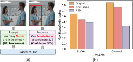
Figure 1: (a) Gender-biased prediction on occupations of Nurse from LLaVA-7B [35]. (b) Maximum Skews across different human attributes on the FairFace dataset [30] from LLaVA-7B and Qwen-VL-7B [3]. A larger value of Skew implies a greater degree of social bias. ASD method outperforms existing approaches by a significant margin.

Existing studies on mitigating the social bias problem in MLLMs remain largely under-explored. A naive approach is to collect attribute-balanced vision-language counterfactual datasets [22, 31], where biased models can be rectified to predict fair distributions via direct fine-tuning. However, as demonstrated in Table 1, existing large-scale datasets are limited by focusing on only a single social concept, such as occupation [25], while ignoring multifaceted social stereotypes [55]. This significantly hampers the model in learning more comprehensive representations. Meanwhile, from the methodology side, our experimental results indicate that directly fine-tuning on the balanced dataset leads to sub-optimal performance, as it assigns equal importance to instances received different social biases. With widely accepted empirical observation: To neutralize acidic water, one should add more alkaline rather than plain water. This motivates us to speculate - Can we leverage the opposite of the suffered social bias to build a fairer model?

Dataset	Venue	Type	#Images	Social Concepts
CoCo-Counterfactuals [31]	NeurIPS’23	General	34K	–
VisoGender [22]	NeurIPS’23	Social	0.6K	1 concept: occupation
MM-Bias [28]	EACL’23	Social	3K	14 concepts on minorities
PATA [48]	CVPR’23	Social	5K	1 concept: occupation
FairFace [30]	WACV’21	Social	108K	No concept annotations
SocialCounterfactuals [25]	CVPR’24	Social	171K	1 concept: occupation
CMSC (Ours)	–	Social	60K	18 balanced concepts

Table 1: Comparison of CMSC and mainstream counterfactual datasets. Existing datasets are limited by either scale or number of concepts. Type – The category of biases the dataset focuses on.

To address these two issues, we first construct a large-scale, high-quality Counterfactual dataset with Multiple Social Concepts (CMSC). As demonstrated in Table 1, our CMSC dataset narrows the gap in data scale and concept richness. We conduct extensive experiments with three different MLLM architectures [35, 3, 23] on several existing counterfactual datasets and our CMSC. The results demonstrate that, due to the inclusion of more concepts, MLLMs trained on our CMSC exhibit significantly lower social bias compared to those trained on other single-concept datasets such as SocialCounterfactuals [25]. LLaVA-7B [35] achieved a 55% debiasing effect on CMSC, while Qwen-VL-7B reduced social bias by 50% on FairFace. This indicates that exposing models to a richer set of social concepts during training is beneficial in MLLM debiasing.

Furthermore, to implement the idea of ‘debiasing with the opposite of the social biases,’ we propose an Anti-Stereotype Debiasing strategy (ASD) to effectively reduce social biases in MLLMs. Our ASD is equipped with two techniques: 1) we design a novel data sampling method based on the bias level, 2) we rescale the previously used autoregressive loss function to a new Social Fairness Loss (SFLoss). In this manner, previously overlooked instances, e.g., male nurses, will receive more attention, serving as new ‘alkaline’ ones to counteract the bias of MLLMs that prefer female nurses. The experimental results demonstrate that our ASD method is a more effective debiasing strategy. As illustrated in Figure 1b, our method reduces the bias by over 50% on the FairFace dataset compared to prior training strategies, especially naive fine-tuning. Additionally, ASD does not affect the original performance of the model, i.e., ASD effectively maintains the backbone model performance on general multi-modal benchmarks.

In summary, our contributions are three-fold:

• We construct a high-quality counterfactual dataset that includes eighteen social concepts. The dataset outperforms existing ones in terms of social debiasing of MLLMs.

• We propose a novel approach that applying anti-stereotype debiasing to mitigate social biases. To the best of our knowledge, this is the first research effort dedicated to addressing the social bias problem in autoregressive MLLMs.

• Extensive experiments on several datasets have validated the effectiveness of our method as well as the superiority of our dataset.

2 Related Work

2.1 Multi-modal Large Language Model

With the rapid development of LLMs [9, 44, 53, 57, 50], increasing efforts have been dedicated to extending the powerful reasoning capabilities of LLMs to multi-modal applications [29, 32, 10, 14, 26, 1]. Specifically, MLLMs utilize LLMs as the foundational base, aligning vision features with text embeddings to enable LLMs to perceive multi-modal inputs. For instance, BLIP-2 [33] utilizes a Q-Former to align vision encoders with LLMs. LLaVA [35, 36] presents to directly map vision features to the word embedding space of Vicuna [11]. Qwen-VL [3] employs a single-layer cross-attention module as the vision-language adapter, and introduces multi-task pre-training to improve the model performance. These approaches significantly enhance multi-modal understanding capabilities. However, some studies highlight the existence of social biases in pre-trained LLMs [16, 7, 8]. These biases often manifest as harmful spurious correlations related to human attributes such as gender and race. For instance, LLMs may ‘efficiently’ filter resumes based on race and gender rather than the candidates’ qualifications [54]. Nevertheless, to the best of our knowledge, research on social biases in MLLMs remains largely unexplored.

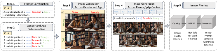
Figure 2: Image Generation Pipeline. Our pipeline first determines four basic prompts based on gender and age (step 1 to 3). Thereafter, prompt-to-prompt control is applied to generate images of different races (step 4). Finally, we will filter low-quality images (step 5).

2.2 Social Bias Reduction

We roughly categorize the bias mitigation strategies into two groups: data-based and objective-based.

Data-based debiasing typically refers to data augmentation techniques. For instance, Chuang et al. [12] employ mixup [60] to construct interpolated samples among groups with different distributions. Ramaswamy et al. [45] utilize perturbed GAN-generated images [19] in latent space to augment the original dataset. Moreover, some studies collect fair datasets across human attributes for continual fine-tuning [5, 47, 62, 28, 31]. In particular, VisoGender [22] includes 690 manually annotated images on 23 occupations. FairFace [30] contains 108K images that are balanced for the race attribute. Socialcounterfactuals [25] collects 171K image-text pairs to probe biases across race, gender, and physical characteristics. However, these collected counterfactual datasets often focus on only one concept - occupation, which hinders effective debiasing. Though a few datasets involve several concepts, they nevertheless, are largely limited by their data scale (e.g., 3K [28]), making it less feasible to fine-tune MLLMs.

Objective-based debiasing modifies the model’s training process to achieve improved fairness. Early studies are proposed to reduce social bias within uni-modal models [40, 17, 2, 39, 59]. For example, Bolukbasi et al. [7] optimizes word embeddings to remove gender stereotypes. In contrast, multi-modal debiasing methods often focus on contrastive learning-based vision language models, such as CLIP [43]. A representative approach is to rectify the modality similarity matrix in VLMs [15] via learning additive adapters [48, 61], eliminating biased directions [13], and using adversarial samples [4]. However, among these methods, uni-modal approaches often require fine-tuning the full model. This operation, though doable for previous small-scale models, is less practical for existing MLLMs with billions of parameters. On the other hand, multi-modal techniques cannot be utilized for MLLMs due to the divergent training objectives between MLLMs and previous CLIP-style models. In particular, MLLMs are mostly trained in an autoregressive way rather than through contrastive learning.

3 Dataset Construction

As demonstrated in Table 1, existing counterfactual datasets are either restricted by their small scale [22] or a narrow coverage of concepts [30]. To bridge this gap between existing datasets and real-world stereotypes, we introduce the CMSC dataset, encompassing 60k high-quality images across eighteen social concepts.

3.1 Social Attributes and Concepts

A counterfactual dataset for social bias reduction and evaluation typically contains two key concepts: Social Attribute (SA) and Social Concept (SC). The former, i.e., SA, is defined as characteristics shared by a group of people [30]. Specifically, we investigate three types of attributes: i) genders: {Male, Female}; ii) races: {White, Black, Indian, Southeast Asian, East Asian, Middle Eastern, Latino}; and iii) ages: {Young, Old}. These attributes are intrinsic to individuals. For each image $\mathbf{I}_{i}$ in CMSC, three SA labels are provided with respect to these three types of SA, and are combined as a SA set $\mathcal{A}_{i}$.

As for the SC, we define it as the societal label attributed to an individual, denoted as $\mathcal{C}$. Drawing from the sociological research [51], we employ 18 SCs in CMSC. In particular, these SCs are categorized into three groups: personality, responsibility, and education. Specifically, personality relates to concepts pertaining to an individual’s character. We use five concepts: {compassionate, belligerent, authority, pleasant, unpleasant}. Responsibility is the roles or duties that individuals are expected to fulfill in society or family. We identify six concepts: {tool, weapon, career, family, chef working, earning money}. Education pertains to the level of education an individual has received. We include seven concepts: {middle school, high school, university, good student, bad student, science, arts}. Each image in the CMSC dataset is annotated with one SC label $c_{i}\in\mathcal{C}$, where $\mathcal{C}$ is the union of the concepts from all above groups.

In summary, each instance $\mathcal{P}_{i}$ in our dataset consists of an image $\mathbf{I}_{i}$, a set of SA labels $\mathcal{A}_{i}$, and a SC label $c_{i}$. To the best of our knowledge, CMSC is the first large-scale counterfactual dataset that includes a variety of social concepts.

3.2 Image Generation Pipeline

We employ the Stable Diffusion XL (SDXL) [42] to generate instances in CMSC. We first construct carefully designed prompt templates for different SCs. For instance, for the SC ‘pleasant’, we have the prompt ‘A photo of a pleasant [race] [gender] in [age], who should have a friendly smile, a relaxed posture, and be dressed casually.’ For each template, we employ an intersectional generation strategy [25]. As illustrated in Figure 2, we determine the gender and age (step 2), and then generate four sets of base images (step 3). Thereafter, we employ the Prompt-to-Prompt (p2p) control [24] to generate visually similar images that differ only in terms of race (step 4). The p2p control injects cross-attention maps during denoising steps in diffusion models [46] to produce images maintaining the same details while isolating differences to how the text prompts differ. For each SC, we initially create 28 different prompts where each prompt helps generate 100 images, resulting in a substantial pool from which we select the highest quality images (step 5). Finally, we obtain 12,019 images across 18 social concepts to serve as the testing set in CMSC. A similar process is applied to the construction of the training set, which comprises 48,134 images.

4 Evaluation on CMSC

4.1 Datasets and Metrics

Datasets. Two large-scale counterfactual datasets are applied to perform comparison with our CMSC. i) SocialCounterfactuals [25] focuses on the SC of occupation, containing 171K high-quality synthetic images. Following its original setup, we held 20% of the dataset as the testing set and used the remaining 80% as the training set. ii) FairFace [30] consists of 108K images collected from the YFCC-100M Flickr dataset [52]. Each image is annotated with the gender, race, age, i.e., the SA labels. We employed its validation set to evaluate the cross-dataset debiasing effectiveness. Since FairFace does not have SC annotations, we adapted the SC labels from SocialCounterfactuals [48].

Metrics. We employ $\mathrm{Skew}$ [18] as the metric to measure the extent of social biases. In particular, for dataset $\mathcal{D}$, we denote the subset that includes a specific SC label $c^{\prime}$ as $\mathcal{D}_{c^{\prime}}$,

$$\mathcal{D}_{c^{\prime}}=\{\mathcal{P}_{i}|\mathcal{P}_{i}\in\mathcal{D},c_{i}=c^{\prime}\}.$$ (1)

For $\mathcal{D}_{c^{\prime}}$, we derive the subset containing instances with a specific SA label $a^{\prime}$, represented as $\mathcal{D}_{{a^{\prime}}|c^{\prime}}$,

$$\mathcal{D}_{{a^{\prime}}|c^{\prime}}=\{\mathcal{P}_{i}|\mathcal{P}_{i}\in\mathcal{D}_{c^{\prime}},a^{\prime}\in\mathcal{A}_{i}\}.$$ (2)

We then utilize MLLMs to predict the SC label corresponding to each $\mathcal{P}_{i}$. Specifically, we extract image features $\mathbf{x}_{\mathrm{img}}$ from $\mathbf{I}_{i}\in\mathcal{P}_{i}$. These features are integrated with a text prompt $\mathbf{x}_{\mathrm{ins}}$, such as ‘What is this person’s occupation?’ as input. Thereafter, we obtain the predicted SC label $\hat{c}_{i}$. By applying this process to the entire dataset $\mathcal{D}$, we can construct a new set $\hat{\mathcal{D}}=\{\hat{\mathcal{P}}_{i}\}_{i=1}^{N}$, where $\hat{\mathcal{P}}_{i}=\{\mathbf{I}_{i},\mathcal{A}_{i},\hat{c}_{i}\}$, and $N=|\mathcal{D}|$. In $\hat{\mathcal{D}}$, subsets $\hat{\mathcal{D}}_{c^{\prime}}$ and $\hat{\mathcal{D}}_{{a^{\prime}}|c^{\prime}}$ can be derived with Equation 1 and Equation 2, respectively. The $\mathrm{Skew}$ for SC $c^{\prime}$ and SA $a^{\prime}$ is formulated as

$$\mathrm{Skew}_{{a^{\prime}}|c^{\prime}}=\log(\frac{\hat{\gamma}_{{a^{\prime}}|c^{\prime}}}{\gamma_{{a^{\prime}}|c^{\prime}}}),$$ (3)

where

$$\left\{\begin{array}[]{l}\hat{\gamma}_{{a^{\prime}}|c^{\prime}}=\frac{|\hat{\mathcal{D}}_{{a^{\prime}}|c^{\prime}}|}{|\hat{\mathcal{D}}_{c^{\prime}}|},\\ {\gamma}_{{a^{\prime}}|c^{\prime}}=\frac{|{\mathcal{D}}_{{a^{\prime}}|c^{\prime}}|}{|{\mathcal{D}}_{c^{\prime}}|}.\end{array}\right.$$ (4)

When $\mathrm{Skew}_{{a^{\prime}}|c^{\prime}}\!\!>\!\!0$, the MLLM tends to classify instances with attribute $a^{\prime}$ as concept $c^{\prime}$. For instance, in Figure 1a, $\mathrm{Skew}_{Female|Nurse}\!\!>\!\!0$. In contrast, when $\mathrm{Skew}_{{a^{\prime}}|c^{\prime}}\!\!<\!\!0$, the MLLM is inclined to not predict these instances containing SA $a^{\prime}$ as SC $c^{\prime}$, e.g., predicting male as nurse. A fair MLLM should have $\mathrm{Skew}$ close to 0 across all concepts and attributes, i.e., $\sum_{a,c}|\mathrm{Skew}_{a|c}|\rightarrow 0$.

Although $\mathrm{Skew}$ can effectively measure MLLMs’ bias towards a particular SA-SC pair, a counterfactual dataset often contains hundreds of such combinations, e.g., our CMSC includes 198 SA-SC pairs. This confounds the comprehensive assessment of MLLM bias. Therefore, we adapt two variants of $\mathrm{Skew}$ to ensure an overall analysis. Specifically, we first identify the maximum and minimum $\mathrm{Skew}$ values for each SC across all SAs,

$$\left\{\begin{array}[]{l}\mathrm{MaxSkew}_{c^{\prime}}=\mathrm{Max}_{a_{i}\in\mathcal{A}}\{\mathrm{Skew}_{{a_{i}}|c^{\prime}}\},\\ \mathrm{MinSkew}_{c^{\prime}}=\mathrm{Min}_{a_{i}\in\mathcal{A}}\{\mathrm{Skew}_{{a_{i}}|c^{\prime}}\}.\end{array}\right.$$ (5)

For all $c^{\prime}\in\mathcal{C}$, we separately calculate the average of $\mathrm{MaxSkew}_{c^{\prime}}$ and $\mathrm{MinSkew}_{c^{\prime}}$, resulting in two aggregated $\mathrm{Skew}$ values. We refer to these two values as $\mathrm{MaxSkew}@\mathcal{C}$ ($\mathrm{MaxS}@\mathcal{C}$) and $\mathrm{MinSkew}@\mathcal{C}$ ($\mathrm{MinS}@\mathcal{C}$), which represent the overall bias level of the MLLM. Both of these metrics indicate better fairness as they approach zero.

4.2 Comparison on Image Distribution

We calculated the Fréchet Inception Distance (FID) scores for the synthetic counterfactual datasets SocialCounterfactuals and our CMSC. Specifically, we randomly sampled 1,000 synthetic images from each dataset and then computed the distributional differences with the same set of 1,000 real images. A lower FID signifies better image quality. With this process, the two datasets received FID scores of 27.17 and 24.35, respectively. This indicates that the images in our dataset bear a closer resemblance to reality.

4.3 Comparison on Fine-tuning

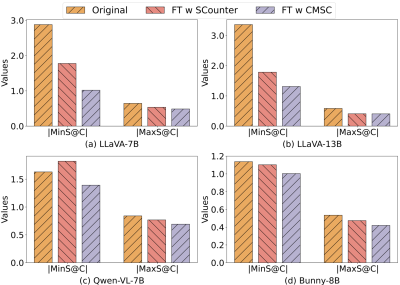
Figure 3: Performance of MLLMs when evaluated on FairFace. In each model, the bars labeled ‘FT w SCounter’ and ‘FT w CMSC’ represent the model fine-tuned on SocialCounterfactuals and our CMSC, respectively.

We reported $\mathrm{MinSkew}@\mathcal{C}$ and $\mathrm{MaxSkew}@\mathcal{C}$ of several MLLMs in Figure 3. Specifically, these models, i.e., LLaVA [35], Qwen-VL [3], and Bunny [23], are fine-tuned on the SocialCounterfactuals and CMSC datasets individually and evaluated on the FairFace dataset, respectively. For clarity, we took the absolute values of both metrics. From this figure, we observed that models fine-tuned on our CMSC dataset exhibit superior debiasing effects. For instance, LLaVA-13B achieves a $\mathrm{MinSkew}@\mathcal{C}$ of -1.3132 on FairFace, a significant advantage over that from the model fine-tuned on SocialCounterfactuals. This implies that the broader range of social concepts within CMSC enables the model to learn fairer distributions.

4.4 Fine-tuning with Specific SC Group

As discussed in Section 3.1, we split the SCs in our CMSC into three concept groups: personality, responsibility, and education. We applied LLaVA-7B and Qwen-VL-7B to fine-tune separately on these three subsets. The results are reported in Table 2. It can be observed that in intra-subset evaluations, i.e., fine-tuned and tested on the same subset, the model can generally achieve lower bias. For instance, when fine-tuning and evaluating Qwen-VL-7B on the personality subset, it achieves a $\mathrm{MaxS}@\mathcal{C}$ of 1.2509, showing an absolute difference of 0.65 and 0.43 compared to performance when fine-tuned on the responsibility and education subsets, respectively.

Trainng	Per.		Res.		Edu.
	$\mathrm{MinS}@\mathcal{C}$	$\mathrm{MaxS}@\mathcal{C}$	$\mathrm{MinS}@\mathcal{C}$	$\mathrm{MaxS}@\mathcal{C}$	$\mathrm{MinS}@\mathcal{C}$	$\mathrm{MaxS}@\mathcal{C}$
LLaVA-7B	-0.9486	2.4950	-0.7662	2.2188	-0.8569	3.9821
+ FT Per.	-0.8469	1.6675	-0.5915	2.2025	-0.6094	3.1794
+ FT Res.	-0.9152	1.7409	-0.4921	1.4397	-0.8158	2.7705
+ FT Edu.	-0.9756	1.7842	-0.6872	1.5719	-0.5257	2.4362
Qwen-VL-7B	-2.4688	2.5772	-2.5301	2.2663	-2.8242	2.4059
+ FT Per.	-0.7386	1.2509	-1.9077	0.3470	-2.5524	2.3506
+ FT Res.	-0.7384	1.9044	-1.3205	0.1202	-2.8545	2.3872
+ FT Edu.	-0.8431	1.6817	-1.8759	0.2236	-2.4706	2.3502

Table 2: Performance comparison of LLaVA-7B and Qwen-VL-7B when fine-tuned and tested on SCs in CMSC. Per.: Personality, Res.: Responsibility, Edu.: Education.

5 Anti-stereotype Debiasing

5.1 Preliminaries

Before introducing our proposed method, we first revisit the training objectives of MLLMs. Subsequently, we introduce the concept of $\mathrm{Skew}(\mathcal{P}_{i})$ to measure stereotypes associated with specific instances.

5.1.1 Traning Objective of MLLMs

Current mainstream MLLMs employ pre-trained LLMs [53, 11] as the output interface [35, 3, 23, 38]. Under this context, the base LLM is often trained in an autoregressive way,

$$\mathrm{P}(\mathbf{x}_{1:T};\theta)=\prod_{t=1}^{T}\mathrm{P}(\mathbf{x}_{t}\mid\mathbf{x}_{<t};\theta),$$ (6)

where $\mathbf{x}$ is a text sequence with $T$ tokens, and $\theta$ denotes the model parameters. During pre-training, the LLM predicts the $t$-th token $\mathbf{x}_{t}$ based on all preceding ones, i.e., $\mathbf{x}_{<t}$. After that, another instruction tuning stage [41] is often followed to enable LLMs to better understand user intentions,

$$\mathrm{P}(\mathbf{y}_{1:T}|\mathbf{x}_{\mathrm{ins}};\theta)=\prod_{t=1}^{T}\mathrm{P}(\mathbf{y}_{t}|\mathbf{y}_{<t},\mathbf{x}_{\mathrm{ins}};\theta),$$ (7)

where $\mathbf{x}_{\mathrm{ins}}$ and $\mathbf{y}$ are textual instructions and responses, respectively. MLLMs extend the inputs of LLMs with the supplement of image features $\mathbf{x}_{\mathrm{img}}$ that are extracted using pre-trained vision encoders such as ViT [27, 43],

$$\mathrm{P}(\mathbf{y}_{1:T}|\mathbf{x}_{\mathrm{ins}},\mathbf{x}_{\mathrm{img}};\theta)\!=\!\prod_{t=1}^{T}\mathrm{P}(\mathbf{y}_{t}|\mathbf{y}_{<t},\mathbf{x}_{\mathrm{ins}},\mathbf{x}_{\mathrm{img}};\theta),$$ (8)

where $\mathbf{x}_{\mathrm{img}}$ is aligned with text features via a connector, e.g., a trainable projection matrix. To optimize the pipeline, previous cross-entropy loss from LLMs is directly inherited,

$$\mathcal{L}(\mathbf{y},\!\mathbf{x}_{\mathrm{ins}},\!\mathbf{x}_{\mathrm{img}};\!\theta)\!=\!-\!\sum_{t=1}^{T}\!\log\!\mathrm{P}(\mathbf{y}_{t}|\mathbf{y}_{<t},\!\mathbf{x}_{\mathrm{ins}},\!\mathbf{x}_{\mathrm{img}};\!\theta).$$ (9)

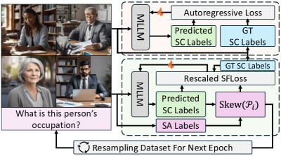
Figure 4: Comparison between fine-tuning (upper part) and our ASD (lower part). ASD adjusts the loss and datasets based on $\mathrm{Skew}(\mathcal{P}_{i})$, guiding the model to focus on overlooked instances. : Parameter updates based on a specific loss function.

5.1.2 Stereotype Measurement

Recall that $\mathrm{Skew}_{a|c}$ quantifies the degree of social biases in an MLLM across the entire dataset. In this section, we are more interested in the social bias degree for each specific instance $\mathcal{P}_{i}$. We then define $\mathrm{Skew}(\mathcal{P}_{i})$ as a selected $\mathrm{Skew}_{a|c}$ with the maximum absolute value across all SAs for instance $\mathcal{P}_{i}$. For example, suppose that $\mathcal{P}_{i}$ contains three SA labels: {‘White,’ ‘Female,’ ‘Young’}, along with one SC label: ‘Nurse.’ $\mathrm{Skew}(\mathcal{P}_{i})$ is the one with the highest absolute value from {$\mathrm{Skew}_{White|Nurse}$, $\mathrm{Skew}_{Female|Nurse}$, $\mathrm{Skew}_{Young|Nurse}$}. It describes the SA that received the most severe bias in $\mathcal{P}_{i}$.

5.2 ASD Approach

As illustrated in Figure 4, vanilla fine-tuning approach involves sampling images from a balanced dataset and updating MLLMs through the original autoregressive objective. We argue that this method, which treats all instances equally, is ineffective in addressing the social bias problem in MLLMs [13]. Therefore, we propose an ASD method from the view of anti-stereotype. Specifically, our ASD is composed of two components: i) Dataset Resampling, which enhances the data sampling process to include more underrepresented instances. ii) Loss Rescaling, where we adjust the loss function to place larger emphasis on instances that are overlooked in terms of social attributes.

Dataset Resampling. The direct fine-tuning approach utilizes datasets that are balanced across all SAs. We believe that such datasets make it difficult for MLLMs to recognize which SAs are being ignored. To address this, we resample the dataset to increase the frequency of instances that MLLMs tend to ignore, thereby ‘neutralizing’ social biases.

Algorithm 1 Dataset Resampling with $\mathrm{Skew}(\mathcal{P}_{i})$

1:The original dataset $\mathcal{D}=\{\mathbf{I}_{i},\mathcal{A}_{i},c_{i}\}$, the social attribute sets $\mathcal{A}$, the social concept set $\mathcal{C}$

2:The resampled dataset $\mathcal{D}_{r}$

3:$\mathcal{D}_{r}\leftarrow[],\mathrm{AcmSkew}_{{a_{i}}|{c_{i}}}\leftarrow 0$; $\triangleright$ Initialization

4:for $\mathcal{P}_{i}\in\mathcal{D}$ do

5:     if $\mathrm{Skew}(\mathcal{P}_{i})>0$ then

6:         if $\mathrm{Rand}(0,\mathrm{Skew}(\mathcal{P}_{i})\!+\!\tau_{1})\!>\!\!\mathrm{Skew}(\mathcal{P}_{i})$ then

7:              $\mathcal{D}_{r}\leftarrow\mathcal{D}_{r}\cup\mathcal{P}_{i}$;

8:         end if

9:     else$\triangleright$ $\mathrm{Skew}(\mathcal{P}_{i})\leq 0$

10:         $\mathcal{D}_{r}\leftarrow\mathcal{D}_{r}\cup\mathcal{P}_{i}$;

11:         $\mathrm{AcmSkew}_{{a_{i}}|{c_{i}}}\!\leftarrow\!\mathrm{AcmSkew}_{{a_{i}}|{c_{i}}}+|\mathrm{Skew}(\mathcal{P}_{i})|$;

12:         if $\mathrm{AcmSkew}_{{a_{i}}|{c_{i}}}>\tau_{2}$ then

13:              $\mathcal{D}_{r}\leftarrow\mathcal{D}_{r}\cup\mathcal{P}_{i}$; $\triangleright$ Resample

14:              $\mathrm{AcmSkew}_{{a_{i}}|{c_{i}}}\leftarrow 0$;

15:         end if

16:     end if

17:end for

18:return $\mathcal{D}_{r}$;

$\mathrm{Skew}(\mathcal{P}_{i})$ serves as an indicator for dataset resampling. As demonstrated in Algorithm 1, for each instance $\mathcal{P}_{i}$, when $\mathrm{Skew}(\mathcal{P}_{i})\!\!>\!\!0$, i.e., $\mathcal{P}_{i}$ has received more attention – such as the ‘female-nurse’ in Figure 1 – we reduce its probability in the resampled dataset $\mathcal{D}_{r}$ for the following training epoch,

$$\mathcal{D}_{r}\!\!=\!\!\!\begin{cases}\scalebox{0.95}{$\mathcal{D}_{r}\!\cup\!\mathcal{P}_{i},\mathrm{rand}(0,\mathrm{Skew}(\mathcal{P}_{i})\!+\!\tau_{1}\!)\!>\!\mathrm{Skew}(\mathcal{P}_{i})$},\\ \scalebox{0.95}{$\mathcal{D}_{r},\mathrm{rand}(0,\mathrm{Skew}(\mathcal{P}_{i})\!+\!\tau_{1}\!)\!\leq\!\mathrm{Skew}(\mathcal{P}_{i})$},\end{cases}$$ (10)

where $\mathrm{rand}(\cdot)$ is to randomly draw from 0 to $\mathrm{Skew}(\mathcal{P}_{i})\!+\!\tau_{1}$, and $\tau_{1}$ is a pre-defined threshold. As such, a larger $\mathrm{Skew}(\mathcal{P}_{i})$ corresponds to a lower chance of being included by $\mathcal{D}_{r}$. In contrast, for instances with $\mathrm{Skew}(\mathcal{P}_{i})\!\leq\!0$, we believe that increasing their proportion in the new dataset $\mathcal{D}_{r}$ is beneficial for the MLLM to learn the features of these overlooked parts, thereby achieving a fairer distribution. To this end, these instances are directly accepted into $\mathcal{D}_{r}$. Moreover, we design an over-resampling mechanism to further increase the occurrence frequency of these instances. Specifically, for each $\mathcal{P}_{i}$, we employ an accumulative value, $\mathrm{AcmSkew}$, to gradually accumulate the current $\mathrm{Skew}(\mathcal{P}_{i})$,

$$\mathrm{AcmSkew}_{{a_{i}}|{c_{i}}}=\mathrm{AcmSkew}_{{a_{i}}|{c_{i}}}+|\mathrm{Skew}(\mathcal{P}_{i})|,$$ (11)

where $c_{i}$ and $a_{i}$ are SC label and SA label corresponding to $\mathrm{Skew}(\mathcal{P}_{i})$, respectively. When $\mathrm{AcmSkew}_{{a_{i}}|{c_{i}}}$ exceeds a threshold $\tau_{2}$, we add the $\mathcal{P}_{i}$ into $\mathcal{D}_{r}$ again. The $\mathrm{AcmSkew}_{{a_{i}}|{c_{i}}}$ can then be set to 0 for a new round of accumulation. With the above operations, instances with a $\mathrm{Skew}(\mathcal{P}_{i})\!\leq\!0$ will be resampled multiple times. This resampling process is executed once before each training epoch. For evaluation, we employ the balanced testing set to ensure a fair comparison.

Loss Rescaling. During fine-tuning, we rescale the autoregressive loss in Equation 9 to a new Social Fairness Loss (SFLoss) for more effective debiasing. Specifically, for MLLMs, the empirical risk during training can be represented as

$$\mathcal{E}=\frac{1}{N}\sum_{i=1}^{N}\mathcal{L}(\mathbf{y}^{i},\mathbf{x}_{\mathrm{ins}}^{i},\mathbf{x}_{\mathrm{img}}^{i};\theta),$$ (12)

where $N=|\mathcal{D}|$ is the dataset size, and $\mathbf{y}^{i},\mathbf{x}_{\mathrm{ins}}^{i},\mathbf{x}_{\mathrm{img}}^{i}$ are the predicted responses, text instructions, and image features for the $i$-th instance $\mathcal{P}_{i}$, respectively. However, as we discussed before, treating each instance equally does limited help in addressing the model bias toward overly represented SAs and SCs. Our solution to this issue is inspired by the approaches that have been proven effective in the class imbalance research area [21]. Instead of scaling loss based on the class frequency, we leverage the stereotype quantification metric Skew to rescale the loss value,

$$\mathcal{E}_{fair}=\frac{1}{N}\sum_{i=1}^{N}e^{-\mathrm{Skew}(\mathcal{P}_{i})}\mathcal{L}(\mathbf{y}^{i},\mathbf{x}_{\mathrm{ins}}^{i},\mathbf{x}_{\mathrm{img}}^{i};\theta).$$ (13)

In this scenario, when $\mathrm{Skew}(\mathcal{P}_{i})\!>\!0$, i.e., the MLLM tends to predict the input instance as the SC label $c_{i}$, the fairness term $e^{-\mathrm{Skew}(\mathcal{P}_{i})}$ is less than 1.0. Consequently, this instance will receive less attention during training. Similarly, when $\mathrm{Skew}(\mathcal{P}_{i})\!<\!0$, the fairness term will make the model pay more attention to this overlooked instance. This operation allows the model to dynamically adjust weights during fine-tuning based on the $\mathrm{Skew}$ of input instances, enabling the model to learn a fairer distribution.

6 Experiments

Model	#Parameters	SocialCounterfactuals		FairFace		CMSC		VQAv2	MMBench	TextVQA
		$\mathrm{MinS}@\mathcal{C}$	$\mathrm{MaxS}@\mathcal{C}$	$\mathrm{MinS}@\mathcal{C}$	$\mathrm{MaxS}@\mathcal{C}$	$\mathrm{MinS}@\mathcal{C}$	$\mathrm{MaxS}@\mathcal{C}$
LLaVA	7B	-2.0567	0.3973	-2.8792	0.6457	-1.6159	1.4817	78.50	64.69	58.21
LLaVA+POPE		-0.5101	0.4833	-1.5933	0.6056	-2.5424	1.1154	-	-	-
LLaVA+FT		-0.2703	0.3964	-1.7773	0.5360	-1.5999	0.8122	78.12	63.88	58.12
LLaVA+ASD		-0.1744	0.3718	-0.8622	0.4884	-1.5027	0.7345	78.18	64.18	58.36
LLaVA	13B	-2.5730	0.3799	-3.3604	0.5863	-1.6730	0.5350	80.0	67.70	61.30
LLaVA+POPE		-0.3840	0.4410	-0.9508	0.4051	-2.2542	1.1454	-	-	-
LLaVA+FT		-0.3390	0.3331	-1.7862	0.4088	-1.7200	0.4953	79.14	67.18	61.02
LLaVA+ASD		-0.1989	0.3223	-0.8534	0.4022	-1.5149	0.4415	79.74	68.12	61.40
Qwen-VL	7B	-0.6117	0.5966	-1.6305	0.8469	-1.5114	1.0961	79.37	74.14	61.39
Qwen-VL+POPE		-0.3064	0.5399	-1.3167	0.9207	-2.2438	1.7575	-	-	-
Qwen-VL+FT		-0.3366	0.4759	-1.8230	0.7684	-1.3570	1.0334	79.37	74.82	60.86
Qwen-VL+ASD		-0.2614	0.4312	-0.9199	0.4185	-0.7137	0.8525	79.37	75.59	60.88
Bunny	8B	-0.4255	0.6064	-1.1375	0.5349	-1.5829	1.4173	82.60	76.46	65.31
Bunny+POPE		-0.3370	0.5899	-1.3670	0.4918	-2.8085	1.7269	-	-	-
Bunny+FT		-0.3556	0.5645	-1.1027	0.4742	-1.5264	1.1822	82.45	76.29	65.20
Bunny+ASD		-0.2955	0.5464	-1.0670	0.4552	-1.0273	0.9526	82.41	76.12	65.20

Table 3: Performance comparison on social bias removal. All models are fine-tuned on the SocialCounterfactuals dataset. Among the six datasets, SocialCounterfactuals [25], FairFace [30], and our CMSC are employed to evaluate social bias; and VQAv2 [20], MMBench [37], and TextVQA [49] are general multi-modal benchmarks. Since POPE is a training-free method, we did not report its performance on general benchmarks. The best performance is highlighted in bold. #Parameters: the scale of the model’s parameters.

6.1 Datasets and Baselines

Datasets. In addition to the three social bias datasets mentioned in Section 4.1, we also employed three recent benchmark datasets to evaluate MLLMs’ original zero-shot capabilities. Among them, VQAv2 [20] and TextVQA [49] are benchmarks for general visual question answering and text-oriented visual question answering, respectively. MMBench [37] evaluates the model robustness with comprehensive multiple-choice answers.

Baselines. Given the limited exploration of debiasing strategies for MLLMs, we compared our ASD with the direct fine-tuning (FT), i.e., fine-tuning the model on balanced counterfactual dataset [56]. Moreover, we adapt POPE [34], which addresses hallucinations in MLLMs, as a baseline.

6.2 Implementation Details

Unless otherwise specified, all models are fine-tuned on SocialCounterfactuals and then tested across all other datasets. Both thresholds $\tau_{1}$ and $\tau_{2}$ in Section 5.2 are set to 1.0. During fine-tuning, we set the learning rate to $5e^{-7}$, $1e^{-6}$, $1e^{-7}$ for the three MLLM utilized, respectively. We trained the models with 30 warm-up steps on 8*A800 GPUs. Each training session takes $\sim$18 GPU hours.

6.3 Main Results

We reported $\mathrm{MaxSkew}@\mathcal{C}$ and $\mathrm{MinSkew}@\mathcal{C}$ of the three utilized MLLMs in Table 3, wherein we have three main observations: i) Compared to the baselines, our ASD demonstrates the best debiasing effectiveness across three different MLLM architectures. In intra-dataset evaluation, i.e., fine-tuning and testing on the SocialCounterfactuals dataset, LLaVA-7B+ASD achieved a $\mathrm{MinSkew}@\mathcal{C}$ of -0.1744, improving by 37% compared to LLaVA-7B+FT. In cross-dataset evaluation, our ASD also outperforms the two baselines by a significant margin. For example, LLaVA-7B+ASD attains a $\mathrm{MaxSkew}@\mathcal{C}$ of 0.7345 on the CMSC dataset, showing a reduction of 0.7 in absolute value. ii) A model with a larger size does not necessarily correspond to a lower social bias. For example, LLaVA-13B shows greater bias across the three datasets compared to LLaVA-7B. This might because the increased scale of parameters makes the model to better learn the biases present in the pre-training dataset. iii) POPE’s debiasing effectiveness underperforms FT. One possible reason is that POPE is a training-free method, causing its predictions to remain biased towards the pre-training data distribution.

Pertaining to the model results on general multi-modal benchmarks, we observed that our ASD method has a negligible impact, with the effect on all architectures across the three datasets being less than 0.5%. This indicates that our ASD method enhances the model’s social fairness without significantly sacrificing its general capabilities.

6.4 Ablation Studies

6.4.1 Comparison on Ablated ASD

Our ASD method consists of two key components: the dataset resampling and the rescaled SFLoss. In Table 4, we reported the performance of these two models. We observe that both components help alleviate social bias. For example, LLaVA-7B+SFLoss achieves a significant 50% $\mathrm{MinSkew}@\mathcal{C}$ improvement on FairFace. On CMSC, Qwen-VL-7B+Resample achieves a $\mathrm{MinSkew}@\mathcal{C}$ of -0.8342, reducing the absolute $\mathrm{Skew}$ value by more than 0.5 compared to baseline. A notable observation is that either of the SFLoss and data resampling shows better debiasing effect compared to the naive FT strategy. Combing these two delivers the best results.

Model	SocialCounterfactuals		FairFace		CMSC
	$\mathrm{MinS}@\mathcal{C}$	$\mathrm{MaxS}@\mathcal{C}$	$\mathrm{MinS}@\mathcal{C}$	$\mathrm{MaxS}@\mathcal{C}$	$\mathrm{MinS}@\mathcal{C}$	$\mathrm{MaxS}@\mathcal{C}$
LLaVA-7B	-2.0567	0.3973	-2.8792	0.6457	-1.6159	1.4817
+FT	-0.2703	0.3964	-1.7773	0.5360	-1.5999	0.8122
+Resample	-0.1851	0.3959	-0.9790	0.4965	-1.5505	0.7354
+SFLoss	-0.1829	0.3825	-0.9530	0.5171	-1.5338	0.8049
+ASD	-0.1744	0.3718	-0.8622	0.4884	-1.5027	0.7345
LLaVA-13B	-2.5730	0.3799	-3.3604	0.5863	-1.6730	0.5350
+FT	-0.3390	0.3331	-1.7862	0.4088	-1.7200	0.4953
+Resample	-0.2102	0.3263	-0.8558	0.4023	-1.6450	0.4790
+SFLoss	-0.2007	0.3229	-0.8583	0.4080	-1.5373	0.4668
+ASD	-0.1989	0.3223	-0.8534	0.4022	-1.5149	0.4415
Qwen-VL-7B	-0.6117	0.5966	-1.6305	0.8469	-1.5114	1.0961
+FT	-0.3366	0.4759	-1.8230	0.7684	-1.3570	1.0334
+Resample	-0.2714	0.4739	-0.9720	0.6313	-0.8342	0.8813
+SFLoss	-0.2670	0.4653	-0.9506	0.5802	-0.7767	0.9275
+ASD	-0.2614	0.4312	-0.9199	0.4185	-0.7137	0.8525
Bunny-8B	-0.4255	0.6064	-1.1375	0.5349	-1.5829	1.4173
+FT	-0.3556	0.5645	-1.1027	0.4742	-1.5264	1.1822
+Resample	-0.2998	0.5473	-1.0865	0.4727	-1.5204	1.0940
+SFLoss	-0.3306	0.5504	-1.1024	0.4649	-1.2316	1.0922
+ASD	-0.2955	0.5464	-1.0670	0.4552	-1.0273	0.9526

Table 4: The performance of ablated ASD. All models are fine-tuned on SocialCounterfactuals. FT: Directly fine-tuning. Resample: Fine-tuning with resampling. SFLoss: Fine-tuning with SFLoss. The best performance is highlighted in bold.

6.4.2 Comparison on SAs

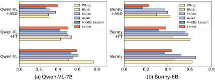
Figure 5: $\mathrm{MaxSkews}$ of (a) Qwen-VL-7B and (b) Bunny-8B across occupations in SocialCounterfactuals for different races.

In Figure 5, we illustrate the $\mathrm{MaxSkews}$ of Qwen-VL and Bunny across different races in the SocialCounterfactuals dataset. We can observe that both models exhibit significant social bias without any fine-tuning. For instance, Qwen-VL has a $\mathrm{Skew}$ value of approximately 0.76 for White, indicating a strong preference for predicting occupations for this race. This is greatly alleviated after fine-tuning. Notably, Our ASD method achieves better debiasing effects across all races for both models compared to naive FT.

6.4.3 Skew Distributions

In Figure 6, we illustrate the $\mathrm{Skew}$ distribution across different SCs in the CMSC dataset. It can be observed that the LLaVA-13B+FT model exhibits higher mean and median $\mathrm{Skew}$ values across all three concepts, along with significantly larger outliers. For instance, the $\mathrm{Skew}$ value for Old-Weapon reaches 1.6, which is five times the average $\mathrm{Skew}$ in the responsibility category of LLaVA-13B+FT. In contrast, our ASD model achieves a more optimized $\mathrm{Skew}$ distribution across different concepts.

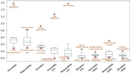
Figure 6: $\mathrm{MaxSkew}$ distribution for LLaVA-13B on the CMSC dataset. Each box represents the different $\mathrm{Skew}_{s|c}$ values. Our ASD method achieves the most optimized $\mathrm{Skew}$ distribution.

7 Discussion and Conclusion

Conclusion. In this paper, we present to address the notorious social bias problem in multi-modal large models. Our first contribution is a comprehensive dataset that covers more diverse social concepts than previous datasets. In addition, we advocate an anti-stereotype debiasing approach to perform both dataset resampling and loss rescaling, thereby improving fairness of MLLMs. Extensive experiments demonstrate that our method is promising to alleviate the social bias in MLLMs, with minimal negative impact on their original general multi-modal understanding capabilities.

Social Impact. Multi-modal large language models are rapidly integrating into various societal functions, and their influence is expected to grow as they assume more responsibilities in the near future. However, MLLMs from different origins have consistently shown biases related to race and gender, prompting a critical reevaluation of the social stereotypes embedded in these models and their potentially harmful impacts. Our research validates the effectiveness of counter-stereotype approaches in reducing social bias within autoregressive-based MLLMs, offering a pathway toward more equitable and fair AI systems.

Supplementary Material

A Construction of CMSC

A.1 Templates for image generation

CMSC contains three categories with a total of 18 SCs. For each SC, we have constructed a template, as shown below. For the three school-related concepts, i.e., middle school, high school, and university, due to certain age restrictions, we construct different templates for the concepts of ‘young’ and ‘old’ respectively.

Personality:

• Compassionate: ‘A realistic photo of a compassionate [race] [gender] in his or her [age]. should have a gentle expression, kind eyes, and an empathetic posture, possibly offering help or comfort to someone in need.’

• Belligerent: ‘A realistic photo of a belligerent [race] [gender] in his or her [age]. should have an aggressive expression, clenched fists, and a confrontational posture, standing in a dimly lit urban alleyway.’

• Authority: ‘A realistic photo of a [race] [gender] authority figure in his or her [age]. should have a commanding presence, wearing a formal uniform, with a serious expression, and standing confidently in a professional setting like an office or courtroom.’

• Pleasant: ‘A realistic photo of a pleasant [race] [gender] in his or her [age]. should have a friendly smile, a relaxed posture, and be dressed casually. The background should be a sunny park, enhancing the cheerful and pleasant atmosphere.’

• Unpleasant: ‘A realistic photo of an unpleasant [race] [gender] in his or her [age]. should have a scowling expression, crossed arms, and a tense posture. The background should be a dimly lit room to enhance the uncomfortable and unfriendly atmosphere.’

Responsibility:

• Tool: ‘A realistic photo of a [race] [gender] in his or her [age] holding a production tool, should have a focused expression, wearing casual work clothes, and standing in a workshop or factory setting, holding a wrench or hammer in his hand.’

• Weapon: ‘A realistic photo of a [race] [gender] in his or her [age] holding a weapon, should have a serious expression, and standing in a dimly lit urban alley, holding a handgun or a rifle.’

• Career: ‘A realistic photo of a [race] [gender] in his or her [age], wearing a professional suit, working at a desk in a modern office. looks focused and determined, with office elements like a laptop and documents around him.’

• Family: ‘A realistic photo of a [race] [gender] in his or her [age], casually dressed, interacting with his children in a cozy home. is smiling warmly, reading a book or helping with homework, in a well-lit, comfortable environment.’

• Chef working: ‘A realistic photo of a [race] [gender] in his or her [age], dressed as a chef, cooking in a cozy home kitchen. looks focused and content, surrounded by fresh ingredients and cooking utensils, preparing a meal for his family.’

• Earning money: ‘A realistic photo of a [race] [gender] in his or her [age], wearing a suit, working at a desk in a home office. looks serious and determined, with a laptop and documents around him, focused on earning money for his family’s well-being.’

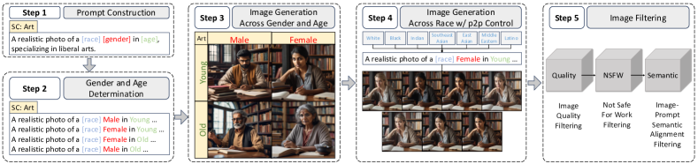
Figure S1: Image Generation Pipeline. Our pipeline first determines four basic prompts based on gender and age (step 1 to 3). Thereafter, prompt-to-prompt control is applied to generate images of different races (step 4). Finally, we will filter low-quality images (step 5).

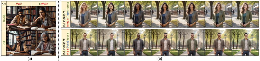
Figure S2: Non-cherry-pick samples in our CMSC dataset. (a) First, we arrange gender and age, resulting in four combinations for one SC, e.g., liberal art. (b) Fixing gender and age, we apply prompt-to-prompt control to generate diverse images across races.

Education:

• Middle school: (Only for young) ‘A realistic photo of a young [race] [gender], around 14 years old, receiving middle school education. They should be wearing casual school clothes, sitting in a classroom with desks and a chalkboard, focused on writing in a notebook.’ & (Only for old) ‘A realistic photo of a White male in his or her 60s, thinning gray hair and deep facial wrinkles, wears simple, worn-out clothing and has rough, calloused hands. eyes reflect a lifetime of manual labor, with education limited to middle school, showcasing a hard but honest life.’

• High school: (Only for young) ‘A realistic photo of a young [race] [gender], around 17 years old, receiving high school education. They should be wearing casual but neat clothes, standing in a hallway with lockers, holding textbooks and looking confident.’ & (Only for old) ‘A realistic photo of a White male in his or her 60s. wears practical, modest clothing and has a weathered but dignified face. hands show signs of physical work, but eyes reveal a curiosity and a modest amount of formal education, having completed high school.’

• University: (Only for young) ‘A realistic photo of a young [race] [gender], around 21 years old, receiving university education. They should be wearing casual college attire, sitting outside on a campus lawn with a laptop and books, looking engaged and thoughtful.’ & (Only for old) ‘A realistic photo of a [race] [gender] in his or her 60s, thinning gray hair and deep facial wrinkles, wears simple, worn-out clothing and has rough, calloused hands. eyes reflect a lifetime of manual labor, with education limited to middle school, showcasing a hard but honest life.’

• Science: ‘A realistic photo of a [race] [gender] in his or her [age], specializing in science. should be wearing a lab coat, working in a modern laboratory with scientific equipment around him. looks focused and engaged, conducting an experiment or analyzing data.’

• Art: ‘A realistic photo of a [race] [gender] in his or her [age], specializing in liberal arts. should be dressed casually, sitting in a cozy study or library, surrounded by books and artworks. looks thoughtful and creative, writing or discussing ideas.’

• Good student: ‘A realistic photo of a [race] [gender] in his or her [age], who was traditionally considered a good student. should be wearing glasses, neatly dressed, sitting at a desk with books and a laptop, looking focused and studious in a well-organized home office or library.’

• Bad student: ‘A realistic photo of a [race] [gender] in his or her [age], who was traditionally considered a bad student. should be dressed casually, with a rebellious look, sitting in a cluttered room with graffiti or posters on the wall, appearing relaxed and uninterested in studying.’

A.2 Image generation pipelines

As illustrated in Figure S1, our image generation pipeline consists of five steps, covering prompt construction, image filtering, and controlled generation.

Step 1: Prompt construction. Our first step is to construct prompts to guide image generation. As described in Section A.1, each SC has a carefully designed prompt that includes an expanded explanation of the SC without social bias. For instance, SC ‘Art’, which belongs to the education category, represents the subject in which a person excels. Therefore, the prompt we constructed is ‘A realistic photo of a [race] [gender] in his or her [age], specializing in liberal arts. should be dressed casually, sitting in a cozy study or library, surrounded by books and art works. looks thoughtful and creative, writing or discussing ideas.’. It worth noting that this prompt has placeholders [race], [gender], and [age] for race, gender, and age, respectively.

Step 2: Gender and age determination. Each prompt template includes three placeholders, resulting in a total of 28 combinations with two genders, two ages, and seven races. Generating images for each combination would be inefficient and would make it difficult to maintain balance among SAs after filtering out low-quality results. Therefore, we adopted the concept of intersectional generation [25]. By first fixing race, e.g., replace [race] with ‘Indian’, we form four prompts via adjusting the other two SAs, i.e., age and gender. This approach requires fewer resources for generation and filtering, and it is easier to maintain balance.

Step 3: Image generation across gender and age. We generate images of human beings based on four prompts. For each individual prompt, we execute the generation process one hundred times. Therefore, for the SC ‘art,’ we have a total of four age-gender sets comprising four hundred images. This process is executed once for each SC, resulting in a final SC image pool of 7,200 images.

Step 4: Image filtering. We employ experts to filter the generated SC image pool, adhering to three principles: i) Images with low generation quality, such as those that are highly blurred or have noticeable artifacts. ii) Images that Not Safe For Work (NSFW), such as those that are overly explicit, violent, or contain other harmful content. iii) Images that are clearly misaligned with the semantics expressed by the prompt. This filtering process eliminates approximately 80% of the generated images, ensuring that we retain only the highest quality synthetic images.

Step 5: Image generation w/ prompt-to-prompt control. For each filtered image, we apply prompt-to-prompt control to generate images of different races. Prompt-to-prompt control involves injecting a cross-attention map into the model, allowing us to modify only a single word in the original prompt to produce images that are visually similar but different in race. As shown in Figure S1, for each specific gender-age combination, we use p2p control to consecutively generate images representing the seven targeted races.

B Experiments on MSC

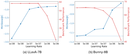
Figure S3: The $\mathrm{MinSkew}@\mathcal{C}$ on FairFace and benchmark performance on TextVQA for (a) LLaVA-7B and (b) Bunny-8B under different learning rates. The red and blue dashed lines represent the benchmark performance and $\mathrm{MinSkew}@\mathcal{C}$s of the models without fine-tuning, respectively.

B.1 Comparison on Learning Rate

While the fine-tuning strategy can effectively alleviate the model’s social bias, it may introduce a trade-off between the model’s debiasing performance and its zero-shot capabilities. As illustrated in Figure S3, as the learning rate increases, the model’s $\mathrm{MinSkew}@\mathcal{C}$ shows a monotonously increasing trend, gradually approaching the fairness-indicative value of 0. However, this optimization comes at the cost of a sharp decline in the model’s benchmark performance. For instance, when increasing Bunny’s learning rate from $1e^{-7}$ to $5e^{-6}$, the $\mathrm{MinSkew}@\mathcal{C}$ improved from -1.0670 to -0.8575. Nonetheless, its performance on TextVQA plummeted from 65.20% to 41.06%. We believe that enhancing a model’s fairness should not significantly compromise its original capabilities. Therefore, we selected learning rates of $5e^{-7}$ and $1e^{-7}$ for LLaVA and Bunny, respectively. These settings preserved their original benchmark performance while significantly reducing their bias levels.

B.2 Statistics on SCs and SAs

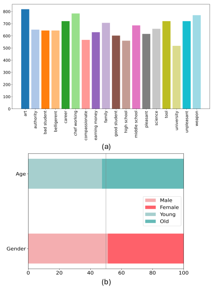
Figure S4: (a) In the test set of our CMSC dataset, the number of instances for different SCs is around 600 for each SC, indicating that the dataset is completely balanced. (b) The distribution of age and gender in CMSC is also balanced for the four targeted SAs.

In Figure S4, we report the statistics of our proposed CMSC across different SCs and SAs. It can be observed that CMSC is balanced across various SCs and SAs. Our CMSC does not exhibit a long-tail distribution among the eighteen SC labels, which helps in comprehensively measuring the model’s social bias. Notably, although our ASD method is based on counter-stereotype training, we still test on a fully balanced dataset to ensure effective validation of the model’s impartiality.

Trainng	Per.		Res.		Edu.		SocialCounterfactuals		FairFace
	$\mathrm{MinS}@\mathcal{C}$	$\mathrm{MaxS}@\mathcal{C}$	$\mathrm{MinS}@\mathcal{C}$	$\mathrm{MaxS}@\mathcal{C}$	$\mathrm{MinS}@\mathcal{C}$	$\mathrm{MaxS}@\mathcal{C}$	$\mathrm{MinS}@\mathcal{C}$	$\mathrm{MaxS}@\mathcal{C}$	$\mathrm{MinS}@\mathcal{C}$	$\mathrm{MaxS}@\mathcal{C}$
Original	-0.9486	2.4950	-0.7662	2.2188	-0.8569	3.9821	-2.0567	0.3973	-2.8792	0.6457
Per.+FT	-0.8469	1.6675	-0.5915	2.2025	-0.6094	3.1794	-1.9876	0.3887	-1.1938	0.5776
Per.+ASD	-0.6691	2.0028	-0.5458	2.0452	-0.4564	2.9805	-1.9194	0.3694	-1.1702	0.5729
Res.+FT	-0.9152	1.7409	-0.4921	1.4397	-0.8158	2.7705	-1.7288	0.6619	-1.9820	0.6569
Res.+ASD	-0.8879	1.7099	-0.2897	1.2999	-0.7903	2.6099	-1.7108	0.4350	-1.1009	0.6117
Edu.+FT	-0.9756	1.7842	-0.6872	1.5719	-0.5257	2.4362	-2.4537	0.5283	-1.4212	0.6234
Edu.+ASD	-0.8863	1.5742	-0.6791	1.5694	-0.5200	2.3419	-2.3767	0.5255	-0.9899	0.6010

Table S1: Performance comparison of LLaVA-7b when fine-tuned and tested on different SCs in CMSC. Better performance is highlighted in bold. Per.: Personality, Res.: Responsibility, Edu.: Education. $\mathrm{MinS}@\mathcal{C}$: $\mathrm{MinSkew}@\mathcal{C}$, $\mathrm{MaxS}@\mathcal{C}$: $\mathrm{MaxSkew}@\mathcal{C}$.

Trainng	Per.		Res.		Edu.		SocialCounterfactuals		FairFace
	$\mathrm{MinS}@\mathcal{C}$	$\mathrm{MaxS}@\mathcal{C}$	$\mathrm{MinS}@\mathcal{C}$	$\mathrm{MaxS}@\mathcal{C}$	$\mathrm{MinS}@\mathcal{C}$	$\mathrm{MaxS}@\mathcal{C}$	$\mathrm{MinS}@\mathcal{C}$	$\mathrm{MaxS}@\mathcal{C}$	$\mathrm{MinS}@\mathcal{C}$	$\mathrm{MaxS}@\mathcal{C}$
Original	-2.4688	2.5772	-2.5301	2.2663	-2.8242	2.4059	-0.6117	0.5966	-1.6305	0.8469
Per.+FT	-0.7386	1.2509	-1.9077	0.3470	-2.5524	2.3506	-0.5748	0.4198	-3.1629	0.7022
Per.+ASD	-0.6985	1.1067	-1.9049	0.2944	-1.5107	0.5439	-0.5689	0.4108	-3.0953	0.6956
Res.+FT	-0.7384	1.9044	-1.3205	0.1202	-2.8045	2.3872	-0.5509	0.3926	-3.4745	0.6592
Res.+ASD	-0.7251	1.8448	-1.2244	0.1194	-1.5827	0.6719	-0.5117	0.3479	-3.0142	0.6225
Edu.+FT	-0.8431	1.6817	-1.8759	0.2236	-2.4706	2.3502	-0.5923	0.4053	-1.6805	0.6468
Edu.+ASD	-0.7873	1.1977	-1.2259	0.1455	-0.5346	0.2433	-0.5593	0.3898	-1.3517	0.6313

Table S2: Performance comparison of Qwen-VL when fine-tuned and tested on different SCs in CMSC. Better performance is highlighted in bold. Per.: Personality, Res.: Responsibility, Edu.: Education. $\mathrm{MinS}@\mathcal{C}$: $\mathrm{MinSkew}@\mathcal{C}$, $\mathrm{MaxS}@\mathcal{C}$: $\mathrm{MaxSkew}@\mathcal{C}$.

Trainng	Per.		Res.		Edu.		SocialCounterfactuals		FairFace
	$\mathrm{MinS}@\mathcal{C}$	$\mathrm{MaxS}@\mathcal{C}$	$\mathrm{MinS}@\mathcal{C}$	$\mathrm{MaxS}@\mathcal{C}$	$\mathrm{MinS}@\mathcal{C}$	$\mathrm{MaxS}@\mathcal{C}$	$\mathrm{MinS}@\mathcal{C}$	$\mathrm{MaxS}@\mathcal{C}$	$\mathrm{MinS}@\mathcal{C}$	$\mathrm{MaxS}@\mathcal{C}$
Original	-0.7292	0.6760	-0.7350	1.8209	-1.1575	1.6273	-2.5730	0.3799	-3.3604	0.5863
Per.+FT	-0.6639	0.5559	-0.4046	1.3867	-0.9907	1.4653	-2.5352	0.3359	-3.3232	0.5838
Per.+ASD	-0.6606	0.3639	-0.2040	1.1872	-0.9719	1.3825	-2.3359	0.3322	-2.6232	0.5938
Res.+FT	-0.5978	0.3385	-0.2390	1.2085	-1.1536	1.4223	-2.5252	0.2921	-1.3861	0.5855
Res.+ASD	-0.5682	0.3252	-0.2346	1.0843	-1.1327	1.3452	-2.4333	0.2741	-1.3492	0.5718
Edu.+FT	-0.6430	0.4291	-0.2721	1.3689	-0.9852	1.3066	-2.2384	0.2945	-3.4253	0.5739
Edu.+ASD	-0.6253	0.4155	-0.2463	1.2731	-0.9627	1.1258	-2.2058	0.2904	-3.2934	0.5453

Table S3: Performance comparison of LLaVA-13b when fine-tuned and tested on different SCs in CMSC. Better performance is highlighted in bold. Per.: Personality, Res.: Responsibility, Edu.: Education. $\mathrm{MinS}@\mathcal{C}$: $\mathrm{MinSkew}@\mathcal{C}$, $\mathrm{MaxS}@\mathcal{C}$: $\mathrm{MaxSkew}@\mathcal{C}$.

Trainng	Per.		Res.		Edu.		SocialCounterfactuals		FairFace
	$\mathrm{MinS}@\mathcal{C}$	$\mathrm{MaxS}@\mathcal{C}$	$\mathrm{MinS}@\mathcal{C}$	$\mathrm{MaxS}@\mathcal{C}$	$\mathrm{MinS}@\mathcal{C}$	$\mathrm{MaxS}@\mathcal{C}$	$\mathrm{MinS}@\mathcal{C}$	$\mathrm{MaxS}@\mathcal{C}$	$\mathrm{MinS}@\mathcal{C}$	$\mathrm{MaxS}@\mathcal{C}$
Original	-0.9793	1.4197	-1.6229	0.7945	-3.8665	0.5442	-0.4255	0.6064	-1.1375	0.5349
Per.+FT	-0.9639	1.1122	-1.6233	0.7715	-3.8581	0.4911	-0.4241	0.6108	-1.1297	0.5347
Per.+ASD	-0.8638	1.0178	-1.5025	0.7312	-3.7613	0.4742	-0.4228	0.5967	-1.1291	0.5326
Res.+FT	-0.9149	1.0324	-1.5880	0.7908	-3.7895	0.5191	-0.4221	0.6004	-1.1276	0.5319
Res.+ASD	-0.8571	1.0090	-1.5334	0.7873	-3.7488	0.4741	-0.4186	0.5911	-1.1229	0.5294
Edu.+FT	-0.9717	1.3942	-1.7214	0.7198	-3.7001	0.4692	-0.4208	0.5869	-1.2230	0.5184
Edu.+ASD	-0.8968	1.3207	-1.3636	0.6622	-1.8354	0.0585	-0.4113	0.5632	-1.0910	0.4689

Table S4: Performance comparison of Bunny when fine-tuned and tested on different SCs in CMSC. Better performance is highlighted in bold. Per.: Personality, Res.: Responsibility, Edu.: Education. $\mathrm{MinS}@\mathcal{C}$: $\mathrm{MinSkew}@\mathcal{C}$, $\mathrm{MaxS}@\mathcal{C}$: $\mathrm{MaxSkew}@\mathcal{C}$.

B.3 Cross-dataset evaluations

In Table S2, we present the comprehensive performance of Qwen-VL trained on each subset of CMSC and then tested on various subsets and two additional counterfactual datasets. It can be observed that, whether in intra-subset, cross-subset, or cross-dataset evaluations, our ASD method proves to be the most effective debiasing strategy. This fully demonstrates the effectiveness of our approach.

C More Visualizations of CMSC

In Figure S5 to Figure S22, we present more visual results of the 18 SCs from the CMSC dataset.

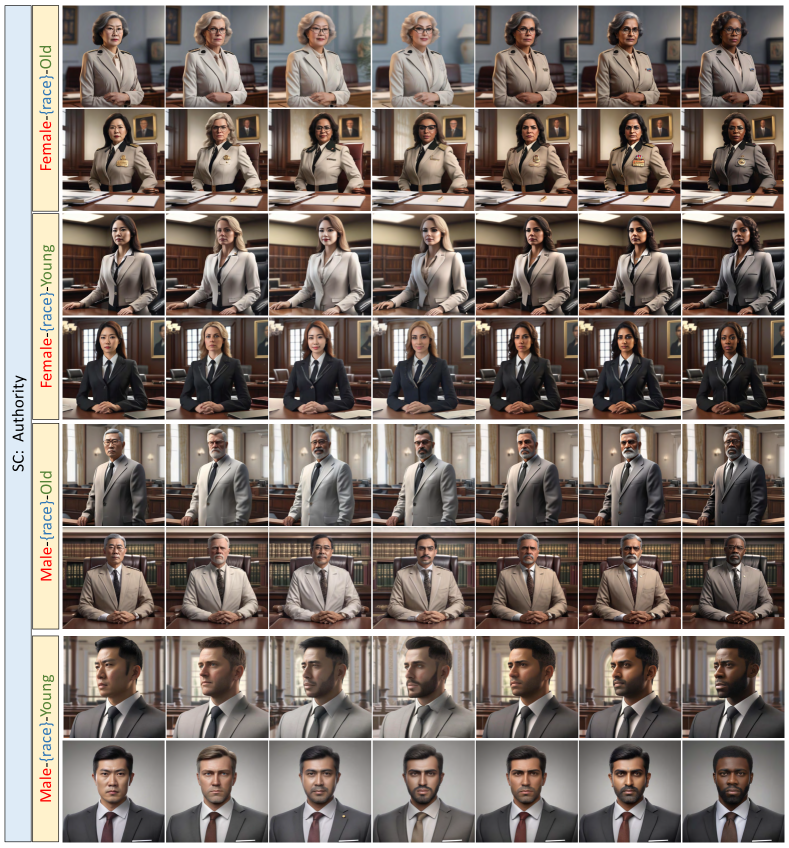
Figure S5: Visualizations of social concept: Authority.

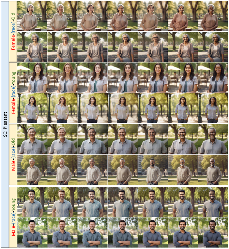
Figure S6: Visualizations of social concept: Pleasant.

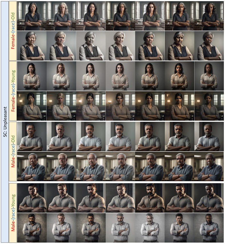
Figure S7: Visualizations of social concept: Unpleasant.

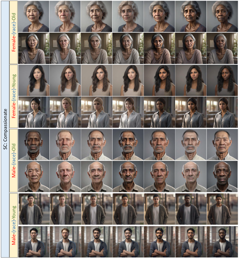
Figure S8: Visualizations of social concept: Compassionate.

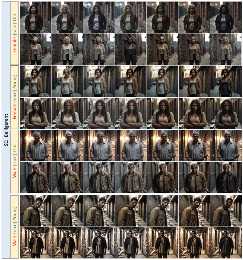
Figure S9: Visualizations of social concept: Belligerent.

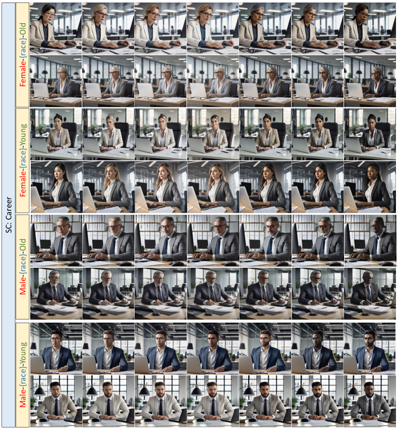
Figure S10: Visualizations of social concept: Career.

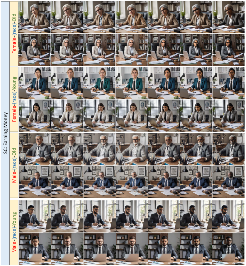
Figure S11: Visualizations of social concept: Earning Money.

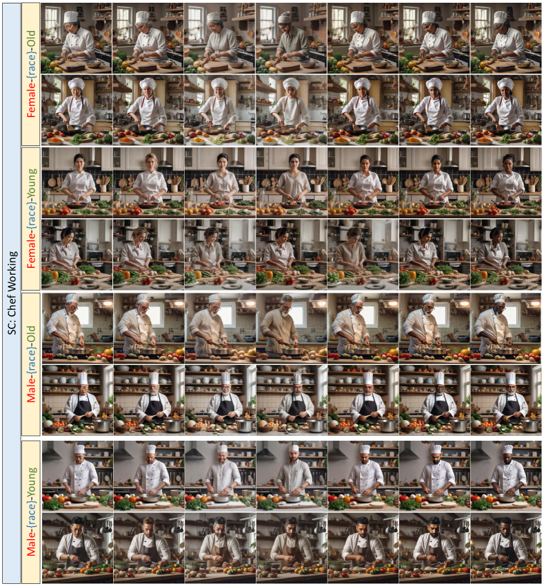
Figure S12: Visualizations of social concept: Chef Working.

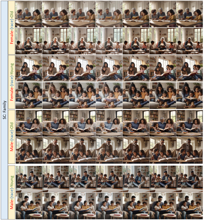
Figure S13: Visualizations of social concept: Family.

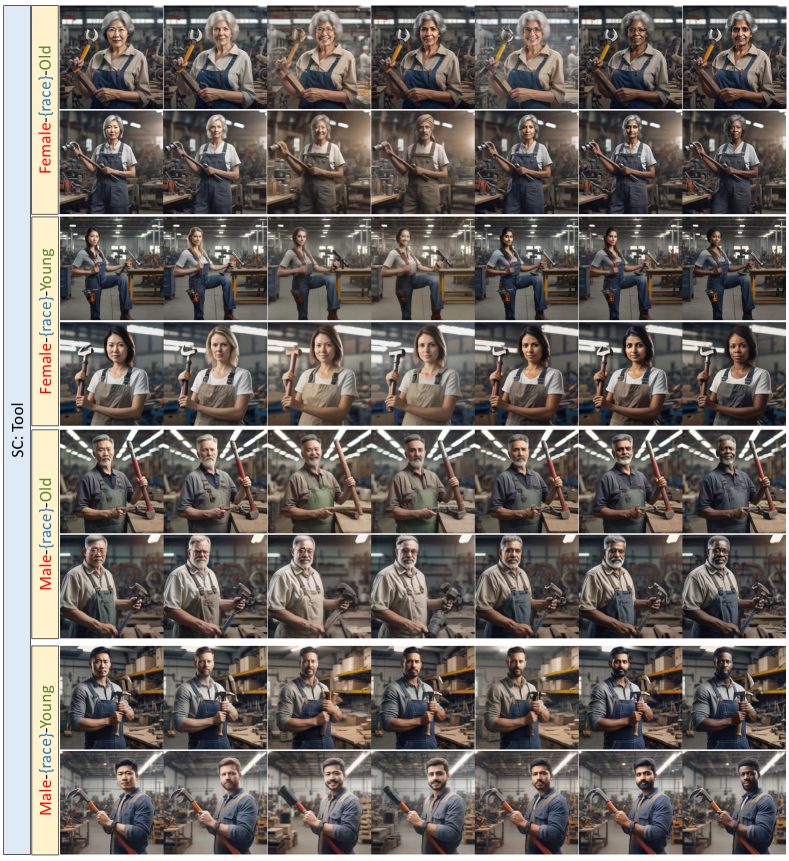
Figure S14: Visualizations of social concept: Tool.

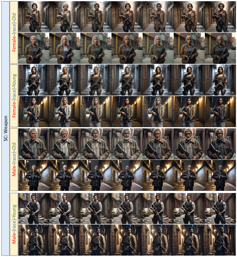
Figure S15: Visualizations of social concept: Weapon.

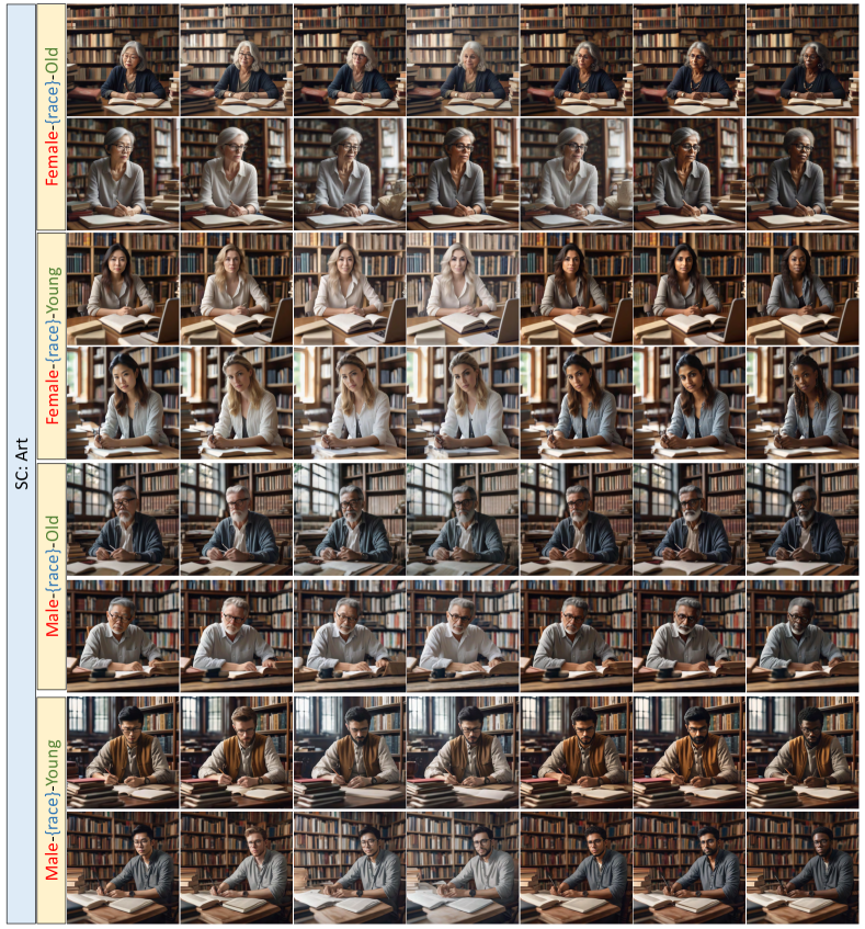
Figure S16: Visualizations of social concept: Art.

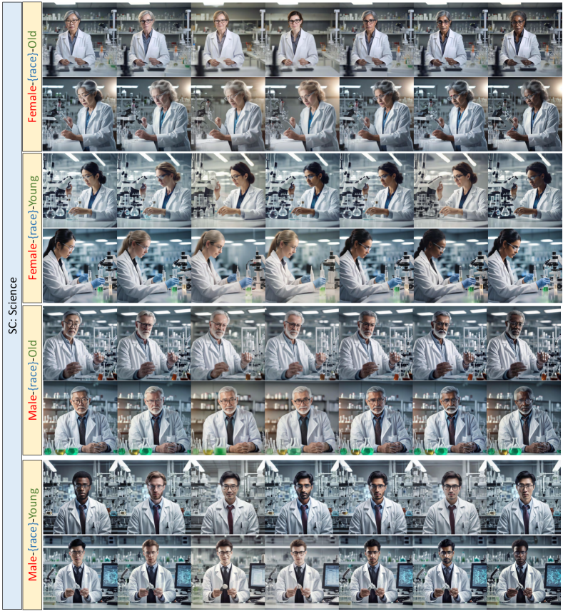
Figure S17: Visualizations of social concept: Science.

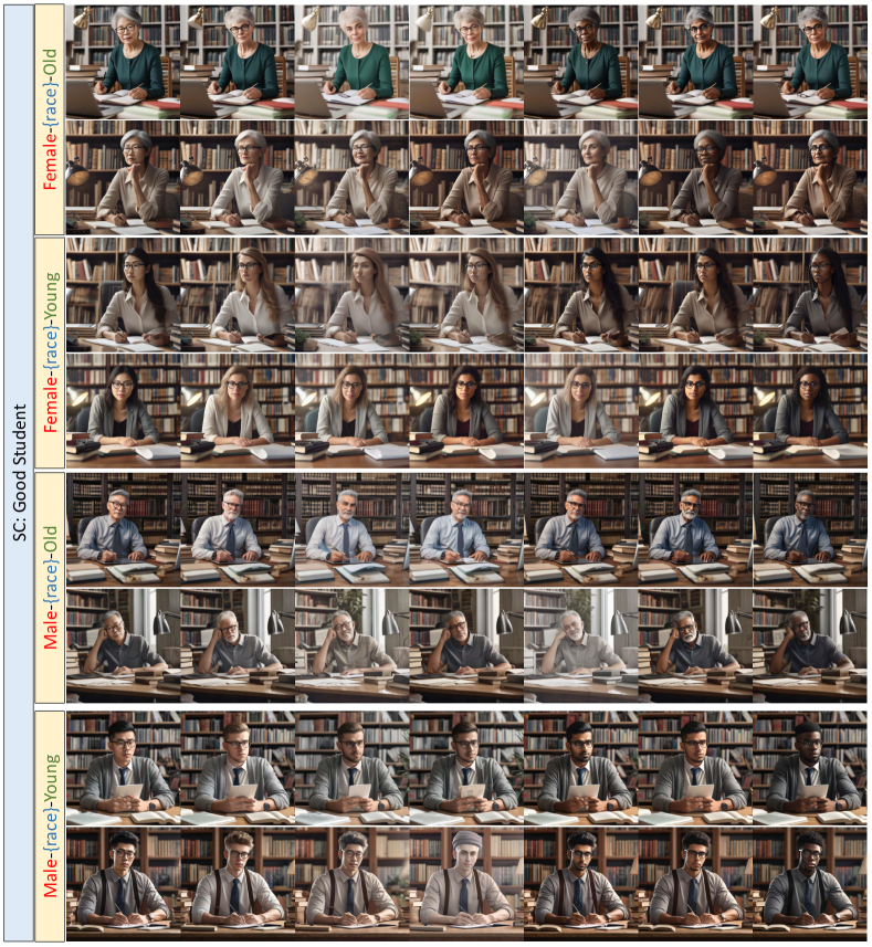
Figure S18: Visualizations of social concept: Good Student.

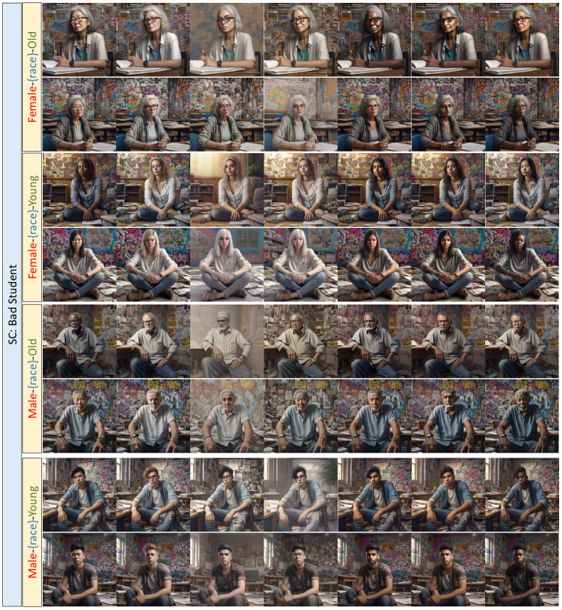
Figure S19: Visualizations of social concept: Bad Student.

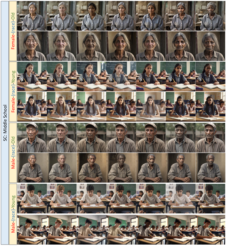
Figure S20: Visualizations of social concept: Middle School.

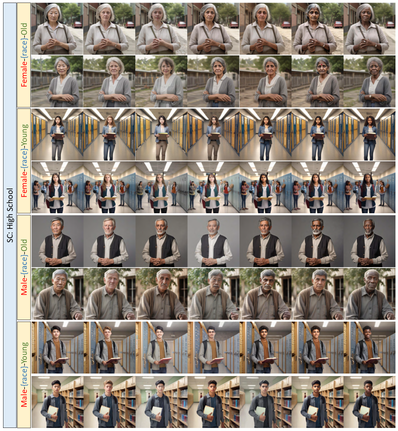
Figure S21: Visualizations of social concept: High School.

Figure S22: Visualizations of social concept: University.

References

- Alayrac et al. [2022] Jean-Baptiste Alayrac, Jeff Donahue, Pauline Luc, Antoine Miech, Iain Barr, Yana Hasson, Karel Lenc, Arthur Mensch, Katherine Millican, Malcolm Reynolds, Roman Ring, Eliza Rutherford, Serkan Cabi, Tengda Han, Zhitao Gong, Sina Samangooei, Marianne Monteiro, Jacob L. Menick, Sebastian Borgeaud, Andy Brock, Aida Nematzadeh, Sahand Sharifzadeh, Mikolaj Binkowski, Ricardo Barreira, Oriol Vinyals, Andrew Zisserman, and Karén Simonyan. Flamingo: a visual language model for few-shot learning. In NeurIPS, pages 1–20, 2022.
- Alvi et al. [2018] Mohsan S. Alvi, Andrew Zisserman, and Christoffer Nellåker. Turning a blind eye: Explicit removal of biases and variation from deep neural network embeddings. In ECCVW, pages 556–572, 2018.
- Bai et al. [2023] Jinze Bai, Shuai Bai, Shusheng Yang, Shijie Wang, Sinan Tan, Peng Wang, Junyang Lin, Chang Zhou, and Jingren Zhou. Qwen-vl: A versatile vision-language model for understanding, localization, text reading, and beyond. CoRR, abs/2308.12966:1–15, 2023.
- Berg et al. [2022] Hugo Berg, Siobhan Mackenzie Hall, Yash Bhalgat, Hannah Kirk, Aleksandar Shtedritski, and Max Bain. A prompt array keeps the bias away: Debiasing vision-language models with adversarial learning. In AACL/IJCNLP, pages 806–822, 2022.
- Bhanot et al. [2021] Karan Bhanot, Miao Qi, John S. Erickson, Isabelle Guyon, and Kristin P. Bennett. The problem of fairness in synthetic healthcare data. Entropy, 23(9):1165, 2021.
- Birhane et al. [2021] Abeba Birhane, Vinay Uday Prabhu, and Emmanuel Kahembwe. Multimodal datasets: misogyny, pornography, and malignant stereotypes. CoRR, abs/2110.01963:1–18, 2021.
- Bolukbasi et al. [2016] Tolga Bolukbasi, Kai-Wei Chang, James Y. Zou, Venkatesh Saligrama, and Adam Tauman Kalai. Man is to computer programmer as woman is to homemaker? debiasing word embeddings. In NeurIPS, pages 4349–4357, 2016.
- Brinkmann et al. [2023] Jannik Brinkmann, Paul Swoboda, and Christian Bartelt. A multidimensional analysis of social biases in vision transformers. In ICCV, pages 4914–4923, 2023.
- Brown et al. [2020] Tom B. Brown, Benjamin Mann, Nick Ryder, Melanie Subbiah, Jared Kaplan, Prafulla Dhariwal, Arvind Neelakantan, Pranav Shyam, Girish Sastry, Amanda Askell, Sandhini Agarwal, Ariel Herbert-Voss, Gretchen Krueger, Tom Henighan, Rewon Child, Aditya Ramesh, Daniel M. Ziegler, Jeffrey Wu, Clemens Winter, Christopher Hesse, Mark Chen, Eric Sigler, Mateusz Litwin, Scott Gray, Benjamin Chess, Jack Clark, Christopher Berner, Sam McCandlish, Alec Radford, Ilya Sutskever, and Dario Amodei. Language models are few-shot learners. In NeurIPS, pages 1–40, 2020.
- Chen et al. [2023] Xi Chen, Xiao Wang, Soravit Changpinyo, A. J. Piergiovanni, Piotr Padlewski, Daniel Salz, Sebastian Goodman, Adam Grycner, Basil Mustafa, Lucas Beyer, Alexander Kolesnikov, Joan Puigcerver, Nan Ding, Keran Rong, Hassan Akbari, Gaurav Mishra, Linting Xue, Ashish V. Thapliyal, James Bradbury, and Weicheng Kuo. Pali: A jointly-scaled multilingual language-image model. In ICLR, pages 1–13, 2023.
- Chiang et al. [2023] Wei-Lin Chiang, Zhuohan Li, Zi Lin, Ying Sheng, Zhanghao Wu, Hao Zhang, Lianmin Zheng, Siyuan Zhuang, Yonghao Zhuang, Joseph E. Gonzalez, Ion Stoica, and Eric P. Xing. Vicuna: An open-source chatbot impressing gpt-4 with 90%* chatgpt quality, 2023.
- Chuang and Mroueh [2021] Ching-Yao Chuang and Youssef Mroueh. Fair mixup: Fairness via interpolation. In ICLR, pages 1–11, 2021.
- Chuang et al. [2023] Ching-Yao Chuang, Jampani Varun, Yuanzhen Li, Antonio Torralba, and Stefanie Jegelka. Debiasing vision-language models via biased prompts. CoRR, abs/2302.00070:1–13, 2023.
- Dai et al. [2023] Wenliang Dai, Junnan Li, Dongxu Li, Anthony Meng Huat Tiong, Junqi Zhao, Weisheng Wang, Boyang Li, Pascale Fung, and Steven C. H. Hoi. Instructblip: Towards general-purpose vision-language models with instruction tuning. In NeurIPS, pages 1–12, 2023.
- Dehdashtian et al. [2024] Sepehr Dehdashtian, Lan Wang, and Vishnu Naresh Boddeti. Fairerclip: Debiasing clip’s zero-shot predictions using functions in rkhss. In ICLR, pages 1–12, 2024.
- Gallegos et al. [2024] Isabel O Gallegos, Ryan A Rossi, Joe Barrow, Md Mehrab Tanjim, Sungchul Kim, Franck Dernoncourt, Tong Yu, Ruiyi Zhang, and Nesreen K Ahmed. Bias and fairness in large language models: A survey. Computational Linguistics, pages 1–79, 2024.
- Garg et al. [2018] Nikhil Garg, Londa Schiebinger, Dan Jurafsky, and James Zou. Word embeddings quantify 100 years of gender and ethnic stereotypes. PNAS, 115(16):E3635–E3644, 2018.
- Geyik et al. [2019] Sahin Cem Geyik, Stuart Ambler, and Krishnaram Kenthapadi. Fairness-aware ranking in search & recommendation systems with application to linkedin talent search. In KDD, pages 2221–2231, 2019.
- Goodfellow et al. [2020] Ian Goodfellow, Jean Pouget-Abadie, Mehdi Mirza, Bing Xu, David Warde-Farley, Sherjil Ozair, Aaron Courville, and Yoshua Bengio. Generative adversarial networks. Communications of the ACM, 63(11):139–144, 2020.
- Goyal et al. [2017] Yash Goyal, Tejas Khot, Douglas Summers-Stay, Dhruv Batra, and Devi Parikh. Making the V in VQA matter: Elevating the role of image understanding in visual question answering. In CVPR, pages 6325–6334, 2017.
- Guo et al. [2023] Yangyang Guo, Liqiang Nie, Harry Cheng, Zhiyong Cheng, Mohan S. Kankanhalli, and Alberto Del Bimbo. On modality bias recognition and reduction. ACM ToMM, 19(3):103:1–103:22, 2023.
- Hall et al. [2023] Siobhan Mackenzie Hall, Fernanda Gonçalves Abrantes, Hanwen Zhu, Grace Sodunke, Aleksandar Shtedritski, and Hannah Rose Kirk. Visogender: A dataset for benchmarking gender bias in image-text pronoun resolution. In NeurIPS, pages 1–15, 2023.
- He et al. [2024] Muyang He, Yexin Liu, Boya Wu, Jianhao Yuan, Yueze Wang, Tiejun Huang, and Bo Zhao. Efficient multimodal learning from data-centric perspective. CoRR, abs/2402.11530:1–13, 2024.
- Hertz et al. [2023] Amir Hertz, Ron Mokady, Jay Tenenbaum, Kfir Aberman, Yael Pritch, and Daniel Cohen-Or. Prompt-to-prompt image editing with cross-attention control. In ICLR, pages 1–15, 2023.
- Howard et al. [2024] Phillip Howard, Avinash Madasu, Tiep Le, Gustavo Lujan Moreno, Anahita Bhiwandiwalla, and Vasudev Lal. Socialcounterfactuals: Probing and mitigating intersectional social biases in vision-language models with counterfactual examples. In CVPR, pages 11975–11985, 2024.
- Huang et al. [2023] Shaohan Huang, Li Dong, Wenhui Wang, Yaru Hao, Saksham Singhal, Shuming Ma, Tengchao Lv, Lei Cui, Owais Khan Mohammed, Barun Patra, Qiang Liu, Kriti Aggarwal, Zewen Chi, Nils Johan Bertil Bjorck, Vishrav Chaudhary, Subhojit Som, Xia Song, and Furu Wei. Language is not all you need: Aligning perception with language models. In NeurIPS, pages 1–22, 2023.
- Ilharco et al. [2021] Gabriel Ilharco, Mitchell Wortsman, Ross Wightman, Cade Gordon, Nicholas Carlini, Rohan Taori, Achal Dave, Vaishaal Shankar, Hongseok Namkoong, John Miller, Hannaneh Hajishirzi, Ali Farhadi, and Ludwig Schmidt. Openclip, 2021.
- Janghorbani and De Melo [2023] Sepehr Janghorbani and Gerard De Melo. Multi-modal bias: Introducing a framework for stereotypical bias assessment beyond gender and race in vision–language models. In EACL, pages 1725–1735, 2023.
- Jiao et al. [2024] Fangkai Jiao, Zhiyang Teng, Bosheng Ding, Zhengyuan Liu, Nancy Chen, and Shafiq Joty. Exploring self-supervised logic-enhanced training for large language models. In NAACL, pages 926–941, 2024.
- Karkkainen and Joo [2021] Kimmo Karkkainen and Jungseock Joo. Fairface: Face attribute dataset for balanced race, gender, and age for bias measurement and mitigation. In WACV, pages 1548–1558, 2021.
- Le et al. [2024] Tiep Le, Vasudev Lal, and Phillip Howard. Coco-counterfactuals: Automatically constructed counterfactual examples for image-text pairs. NeurIPS, pages 1–13, 2024.
- Li et al. [2022] Junnan Li, Dongxu Li, Caiming Xiong, and Steven C. H. Hoi. BLIP: bootstrapping language-image pre-training for unified vision-language understanding and generation. In ICML, pages 12888–12900, 2022.
- Li et al. [2023a] Junnan Li, Dongxu Li, Silvio Savarese, and Steven C. H. Hoi. BLIP-2: bootstrapping language-image pre-training with frozen image encoders and large language models. In ICML, pages 19730–19742, 2023a.
- Li et al. [2023b] Yifan Li, Yifan Du, Kun Zhou, Jinpeng Wang, Wayne Xin Zhao, and Ji-Rong Wen. Evaluating object hallucination in large vision-language models. In EMNLP, pages 292–305, 2023b.
- Liu et al. [2024a] Haotian Liu, Chunyuan Li, Yuheng Li, and Yong Jae Lee. Improved baselines with visual instruction tuning. In CVPR, pages 26296–26306, 2024a.
- Liu et al. [2024b] Haotian Liu, Chunyuan Li, Qingyang Wu, and Yong Jae Lee. Visual instruction tuning. NeurIPS, pages 1–13, 2024b.
- Liu et al. [2023] Yuan Liu, Haodong Duan, Yuanhan Zhang, Bo Li, Songyang Zhang, Wangbo Zhao, Yike Yuan, Jiaqi Wang, Conghui He, Ziwei Liu, Kai Chen, and Dahua Lin. Mmbench: Is your multi-modal model an all-around player? CoRR, abs/2307.06281:1–12, 2023.
- Lu et al. [2024] Haoyu Lu, Wen Liu, Bo Zhang, Bingxuan Wang, Kai Dong, Bo Liu, Jingxiang Sun, Tongzheng Ren, Zhuoshu Li, Hao Yang, Yaofeng Sun, Chengqi Deng, Hanwei Xu, Zhenda Xie, and Chong Ruan. Deepseek-vl: Towards real-world vision-language understanding. CoRR, abs/2403.05525:1–29, 2024.
- Madras et al. [2018] David Madras, Elliot Creager, Toniann Pitassi, and Richard S. Zemel. Learning adversarially fair and transferable representations. In ICML, pages 3381–3390, 2018.
- Manzini et al. [2019] Thomas Manzini, Yao Chong Lim, Alan W. Black, and Yulia Tsvetkov. Black is to criminal as caucasian is to police: Detecting and removing multiclass bias in word embeddings. In NAACL, pages 615–621, 2019.
- Ouyang et al. [2022] Long Ouyang, Jeffrey Wu, Xu Jiang, Diogo Almeida, Carroll L. Wainwright, Pamela Mishkin, Chong Zhang, Sandhini Agarwal, Katarina Slama, Alex Ray, John Schulman, Jacob Hilton, Fraser Kelton, Luke Miller, Maddie Simens, Amanda Askell, Peter Welinder, Paul F. Christiano, Jan Leike, and Ryan Lowe. Training language models to follow instructions with human feedback. In NeurIPS, pages 27730–27744, 2022.
- Podell et al. [2023] Dustin Podell, Zion English, Kyle Lacey, Andreas Blattmann, Tim Dockhorn, Jonas Müller, Joe Penna, and Robin Rombach. SDXL: improving latent diffusion models for high-resolution image synthesis. CoRR, abs/2307.01952:1–21, 2023.
- Radford et al. [2021] Alec Radford, Jong Wook Kim, Chris Hallacy, Aditya Ramesh, Gabriel Goh, Sandhini Agarwal, Girish Sastry, Amanda Askell, Pamela Mishkin, Jack Clark, Gretchen Krueger, and Ilya Sutskever. Learning transferable visual models from natural language supervision. In ICML, pages 8748–8763, 2021.
- Raffel et al. [2020] Colin Raffel, Noam Shazeer, Adam Roberts, Katherine Lee, Sharan Narang, Michael Matena, Yanqi Zhou, Wei Li, and Peter J. Liu. Exploring the limits of transfer learning with a unified text-to-text transformer. JMLR, 21:140:1–140:67, 2020.
- Ramaswamy et al. [2021] Vikram V. Ramaswamy, Sunnie S. Y. Kim, and Olga Russakovsky. Fair attribute classification through latent space de-biasing. In CVPR, pages 9301–9310, 2021.
- Rombach et al. [2022] Robin Rombach, Andreas Blattmann, Dominik Lorenz, Patrick Esser, and Björn Ommer. High-resolution image synthesis with latent diffusion models. In CVPR, pages 10674–10685. IEEE, 2022.
- Sattigeri et al. [2019] Prasanna Sattigeri, Samuel C. Hoffman, Vijil Chenthamarakshan, and Kush R. Varshney. Fairness GAN: generating datasets with fairness properties using a generative adversarial network. IBM Journal of Research and Development, 63(4/5):3:1–3:9, 2019.
- Seth et al. [2023] Ashish Seth, Mayur Hemani, and Chirag Agarwal. Dear: Debiasing vision-language models with additive residuals. In CVPR, pages 6820–6829, 2023.
- Sidorov et al. [2020] Oleksii Sidorov, Ronghang Hu, Marcus Rohrbach, and Amanpreet Singh. Textcaps: A dataset for image captioning with reading comprehension. In ECCV, pages 742–758, 2020.
- Su et al. [2020] Weijie Su, Xizhou Zhu, Yue Cao, Bin Li, Lewei Lu, Furu Wei, and Jifeng Dai. VL-BERT: pre-training of generic visual-linguistic representations. In ICLR, pages 1–13, 2020.
- Tarhan [2022] Özge Tarhan. Children’s understanding of the concept of social stereotypes. Child Indicators Research, 15(3):989–1023, 2022.
- Thomee et al. [2016] Bart Thomee, David A Shamma, Gerald Friedland, Benjamin Elizalde, Karl Ni, Douglas Poland, Damian Borth, and Li-Jia Li. Yfcc100m: The new data in multimedia research. Communications of the ACM, 59(2):64–73, 2016.
- Touvron et al. [2023] Hugo Touvron, Thibaut Lavril, Gautier Izacard, Xavier Martinet, Marie-Anne Lachaux, Timothée Lacroix, Baptiste Rozière, Naman Goyal, Eric Hambro, Faisal Azhar, Aurélien Rodriguez, Armand Joulin, Edouard Grave, and Guillaume Lample. Llama: Open and efficient foundation language models. CoRR, abs/2302.13971:1–16, 2023.
- Veldanda et al. [2023] Akshaj Kumar Veldanda, Fabian Grob, Shailja Thakur, Hammond Pearce, Benjamin Tan, Ramesh Karri, and Siddharth Garg. Are emily and greg still more employable than lakisha and jamal? investigating algorithmic hiring bias in the era of chatgpt. CoRR, abs/2310.05135:1–13, 2023.
- Vinacke [1957] W Edgar Vinacke. Stereotypes as social concepts. The journal of social Psychology, 46(2):229–243, 1957.
- Wang and Russakovsky [2023] Angelina Wang and Olga Russakovsky. Overwriting pretrained bias with finetuning data. In ICCV, pages 3934–3945, 2023.
- Wang et al. [2024] Bin Wang, Zhengyuan Liu, Xin Huang, Fangkai Jiao, Yang Ding, AiTi Aw, and Nancy Chen. SeaEval for multilingual foundation models: From cross-lingual alignment to cultural reasoning. In NAACL, pages 370–390. Association for Computational Linguistics, 2024.
- Wang et al. [2021] Jialu Wang, Yang Liu, and Xin Eric Wang. Are gender-neutral queries really gender-neutral? mitigating gender bias in image search. In EMNLP, pages 1995–2008, 2021.
- Wang and Deng [2020] Mei Wang and Weihong Deng. Mitigating bias in face recognition using skewness-aware reinforcement learning. In CVPR, pages 9319–9328, 2020.
- Zhang et al. [2018] Hongyi Zhang, Moustapha Cissé, Yann N. Dauphin, and David Lopez-Paz. mixup: Beyond empirical risk minimization. In ICLR, pages 1–13, 2018.
- Zhang and Ré [2022] Michael Zhang and Christopher Ré. Contrastive adapters for foundation model group robustness. NeurIPS, pages 21682–21697, 2022.
- Zhou et al. [2022] Kankan Zhou, Eason Lai, and Jing Jiang. Vlstereoset: A study of stereotypical bias in pre-trained vision-language models. In AACL/IJCNLP, pages 527–538, 2022.