Resonant Forbidden CP Asymmetry from Soft Leptons

Abstract

To explain the baryon asymmetry in the early universe via leptogenesis, quantum corrections to new particles are commonly invoked to generate the necessary CP asymmetry. We demonstrate, however, that a large CP asymmetry can already arise from Standard Model leptons. The mechanism relies on resummation of soft leptons at finite temperatures. The CP asymmetry, which is kinetically forbidden in vacuum, can be resonantly enhanced from thermally resummed leptons by seven orders of magnitude. Contrary to the resonance from exotic particles, we show that the resonant enhancement from soft leptons is protected by controlled widths under finite-temperature perturbation theory. We quantify such CP asymmetries in leptogenesis with secluded flavor effects and comment on the significance and application. The mechanism exploits the maximal role of leptons themselves, featuring low-scale leptogenesis, minimal model buildings and dark matter cogenesis.

Introduction.— The baryon asymmetry in the universe (BAU) remains a fundamental question in the Standard Model (SM) of particle physics and cosmology Planck:2018vyg . Baryogenesis via leptogenesis is a simple mechanism to create a baryon asymmetry in the early universe Fukugita:1986hr ; Luty:1992un ; Covi:1996wh . A common ingredient of CP asymmetries necessary for the BAU problem is the onshell cuts arising from quantum loop diagrams of mixed particles. This underlies current leptogenesis, where onshell cuts are present in loop diagrams of flavored neutrinos Giudice:2003jh ; Buchmuller:2004nz ; Davidson:2008bu ; Fong:2012buy or mixed scalars Covi:1996fm ; Ma:1998dx ; Dick:1999je ; Murayama:2002je .

While the SM leptons are the basic container for lepton-baryon processing via sphaleron at high temperatures Kuzmin:1985mm , the requisite amount of CP asymmetries for sphaleron processing insofar is not induced by lepton mixing itself but is instead generated by new particle mixing. Given that new physics (NP) interactions in leptogenesis unavoidably induce certain mixing for lepton flavors, onshell cuts from lepton loop diagrams may also generate CP asymmetries. In vacuum, however, there is no kinetic cut making particles onshell from lepton loop diagrams, since the loop particles are massive while the SM lepton doublets are massless.

Nevertheless, particles in a thermal plasma are of statistical nature. Loop particles being onshell can correspond not only to emission processes but also to absorption from the plasma, with the probability proportional to distribution functions Weldon:1983jn . Such plasma-induced effects have been considered in loop diagrams of neutrinos and scalars by using the Schwinger–Keldysh Closed-Time-Path (CTP) formalism Chou:1984es ; Calzetta:1986cq ; Berges:2004yj , such as unflavored leptogenesis Garny:2009qn ; Beneke:2010wd ; Garbrecht:2010sz ; Garny:2010nj , flavored leptogenesis Beneke:2010dz ; Drewes:2012ma , resonant leptogenesis Garbrecht:2011aw ; Garny:2011hg ; BhupalDev:2014oar and scalar decay Frossard:2012pc ; Garbrecht:2012qv ; Hambye:2016sby . Noticeably, some of these plasma-induced CP asymmetries can work as the only CP-violating source at finite temperatures, which is otherwise forbidden in vacuum.

While plasma-induced CP asymmetries may already arise from leptons at finite temperatures, there is a dearth of investigations into how such CP asymmetries arise from leptons, and particularly to what extent the CP asymmetry can be generated. One difficulty comes from applying the Kadanoff-Baym (KB) mixing equations Prokopec:2003pj ; Prokopec:2004ic to SM lepton flavors Garbrecht:2012pq . It is known that the unmixed KB equation is much more difficult to manage than the conventional Boltzmann equation used in most leptogenesis. The intrinsic complexity of lepton KB mixing equations further makes the generation and evolution of CP asymmetries more challenging to compute. Moreover, the KB mixing equations introduce nontrivial time-dependent matrix structures, making the plasma-induced CP asymmetry from lepton mixing difficult to trace.

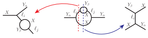
Figure 1: Left: an $S$-matrix glimpse of the resonant forbidden CP asymmetry from the cuts of lepton self-energy diagram. Middle: a two-loop diagram for CP violation in the CTP formalism, where the red cutting line has a qualitative correspondence to the left diagram. Right: a $t$-channel scattering process mediated by massless leptons, which can be induced by the blue cutting line of the two-loop diagram.

In this Letter, we introduce the concept of forbidden CP asymmetries from soft-lepton mixing and provide a simple approach to calculate the forbidden CP asymmetries. This approach circumvents the lepton KB mixing equations and focuses on the accompanying asymmetries in the NP sector. While indirect, the approach offers a simple picture of how the CP asymmetry is generated after resumming leptons at finite temperatures and how resonant enhancement appear. It also allows easy implementation and generalization in leptogenesis. The resonant forbidden CP asymmetries can either work as a new mechanism for leptogenesis where no vacuum cuts exist, or contribute as an irreducible source to leptogenesis where cuts already exist in vacuum.

The $\boldsymbol{S}$-matrix picture.— Let us first present a simple picture of how CP asymmetries arise from thermally corrected leptons, and get a glimpse of the resonantly enhanced forbidden CP asymmetry. In the $S$-matrix formalism, an onshell cut from SM lepton self-energy can be described by the left diagram in Fig. 1. Consider the prototype of Yukawa interactions in leptogenesis: $y^{\prime}_{i\alpha}\bar{\ell}_{i}XY_{\alpha}+\rm h.c.$, with a single fermion (scalar) $X$, multi-flavor scalars (fermions) $Y_{\alpha}$, and the SM leptons $\ell$. The Yukawa couplings $y^{\prime}_{i\alpha}$ introduce one of the necessary CP-violating phases (Yukawa phase) from the NP sector. For massive $X$ and $Y$, it is straightforward to check that no kinetic phase (onshell $X$ and $Y_{\beta}$) can arise from the loop diagram in vacuum. At finite temperatures, however, the emission and absorption of $X$ and $Y_{\beta}$ carry statistic distributions. Particles $X,Y_{\beta}$ in the lepton loop diagram have certain probability to be onshell, depending on the distributions of $X$ and $Y_{\beta}$. Following the standard calculation of the $S$-matrix amplitude between $X\to Y_{\alpha}+\ell_{j}$ and its CP-conjugated process up to the order shown in the left diagram of Fig. 1, a $Y_{\alpha}$ asymmetry will be generated.

When computing the decay and $t$-scattering channels mediated by the massless propagator $\ell_{i}$ via the vacuum $S$-matrix formalism, we will encounter infrared (IR) divergence in the limit $p_{\ell}\to 0$. Such IR divergence arises from massless leptons at high temperatures, which usually indicates the breakdown of perturbation expansion. One known technique to cure this IR divergence is the Hard-Thermal-Loop (HTL) resummation Braaten:1989mz ; Carrington:1997sq ; Bellac2000 , where thermal emission, propagation and absorption with soft momentum $p\sim gT$ or $p_{0}^{2}-|\vec{p}|^{2}\sim g^{2}T^{2}$ should be resummed over one-particle-irreducible (1PI) self-energy diagrams. Here $g$ denotes the weak coupling in the theory and $T$ the background temperature. The HTL resummation induces a temperature-dependent mass, which works as an effective regulator to remove the IR divergence. This serves as the first motivation for soft-lepton resummation.

If we simply treat the resummation of leptons by inserting the thermal masses with the modified dispersion relation $p^{2}\sim\tilde{m}^{2}$ into the propagator $\ell_{i}$ and the external state $\ell_{j}$, we will obtain an asymmetry of the $Y_{\alpha}$ number density scaling like

$$n_{Y_{\alpha}}-n_{\bar{Y}_{\alpha}}\propto\mathcal{O}(y^{\prime 4})\times\frac{m_{X}^{2}}{\tilde{m}_{j}^{2}-\tilde{m}_{i}^{2}}\,.$$ (1)

Such scaling is generically expected from self-energy cuts in conventional leptogenesis Giudice:2003jh ; Buchmuller:2004nz ; Davidson:2008bu ; Fong:2012buy . Here the asymmetry is generated at quartic order of Yukawa couplings, the vacuum mass $m_{X}$ is introduced by dimensional arguments, and Weldon:1982bn

$$\tilde{m}_{i}^{2}=\left(\frac{3}{32}g_{2}^{2}+\frac{1}{32}g_{1}^{2}+\frac{1}{16}y_{i}^{2}\right)T^{2}\,,$$ (2)

denotes the squared thermal mass of lepton flavor $i$ with gauge couplings $g_{2},g_{1}$ and the charged-lepton Yukawa coupling $y_{i}$. The difference in the denominator of Eq. (1) cancels the dependence on gauge couplings, giving rise to a maximal enhancement $1/(y_{\mu}^{2}-y_{e}^{2})\gtrsim 4.4\times 10^{7}$ at $T\lesssim m_{X}$. The enhancement mimics the mass degeneracy between two neutrinos or scalars in resonant leptogenesis Pilaftsis:2003gt ; Pilaftsis:2005rv . We will show in this Letter that the enhancement is protected by a controlled cancellation even after the thermal widths of leptons are included in finite-temperature perturbation theory.

The evolution of the CP asymmetry generated from the left diagram of Fig. 1 may be quantified by Boltzmann equations with $S$-matrix amplitudes. However, since the CP asymmetry is a thermal quantum-statistical effect, using the the semi-classical Boltzmann equations can lead to inconsistent conclusions. This can be inferred from the two-loop diagram in the middle of Fig. 1, where decay on the left of Fig. 1 originates from the red cutting line and $t$-channel scattering on the right is induced by the blue cutting line. The scattering channel inherited from the middle diagram contains both onshell and offshell lepton propagation. The CP asymmetry from the onshell mode is essential to guarantee CPT invariance and unitarity Giudice:2003jh ; Frossard:2012pc . This cancellation avoids the double-counting issue which, in contrast, occurs in Boltzmann equations if one only considers decay and inverse decay from the left diagram Kolb:1979qa .

For practical calculations, the optical theorem may be formulated in finite-temperature field theory so that one can insert proper Green’s functions in the left diagram to estimate the forbidden CP asymmetry Kobes:1990ua ; Garny:2010nj ; Frossard:2012pc ; Hambye:2016sby ; Li:2020ner ; Li:2021tlv . Nevertheless, the optical theorem in finite-temperature field theory, also known as thermal cutting/circling rules Kobes:1985kc ; Kobes:1986za , does not always provide simpler ways to calculate the CP asymmetry, and these calculations could still miss the contribution from onshell scattering that has a canceling effect on the decay-induced CP asymmetry. An important feature in this respect is that the out-of-equilibrium condition provided by the decay product $Y_{\alpha}$ is not sufficient to generate a nonzero forbidden CP asymmetry, as will be shown below by using the 2-loop diagram in the CTP formalism.

CP asymmetry in the CTP formalism— The resummation of soft leptons discussed above is not only motivated by IR divergence and the associated perturbation issue, but also the built-in procedure in the CTP formalism. The collision rates in the KB equation come from the functional derivative of the two-particle-irreducible (2PI) effective action Calzetta:1986cq ; Berges:2004yj , which is formed by closed loops with full propagators. As shown in Fig. 2, the resummation of leptons includes the 1PI diagrams from flavor-conserving SM contributions and flavor-changing NP corrections.

To proceed, let us consider for definiteness a simple Yukawa interaction $y^{\prime}_{ij}\bar{\ell}_{i}\tilde{\phi}P_{R}\chi_{j}+\rm h.c.$ added to the SM, where $\tilde{\phi}\equiv i\sigma_{2}\phi^{*}$ is a gauge $SU(2)_{L}$ scalar doublet and two fermion flavors $P_{R}\chi_{j}\equiv(1+\gamma_{5})\chi_{j}/2$ are attached. In the basis where the charged-lepton Yukawa and $\chi$-mass matrices are diagonal, the Yukawa interactions above induce lepton flavor mixing. To quantify the impacts of the forbidden CP asymmetry in leptogenesis, we consider an example where the total lepton number $L_{\rm tot}=L_{\rm SM}+L_{\chi}$ is conserved or approximately conserved during the main epoch of leptogenesis. In this example, leptogenesis is triggered via the $B+L_{\rm SM}$ violating but $B-L_{\rm SM}$ conserving sphaleron process, once an asymmetry is generated and secluded in the $\chi$ sector that satisfies $B-L_{\rm SM}\approx L_{\chi}$. This realization mimics the idea of hiding lepton (or baryon) numbers in the dark sector, where dark/secluded flavor effects can retain a net asymmetry from lepton- (baryon-) number conserving processes Akhmedov:1998qx ; Dick:1999je ; Davoudiasl:2010am ; Cheung:2011if ; Elor:2018twp .

Consider the situation where $\chi_{1}$ is out of equilibrium while $\chi_{2}$ keeps in thermal equilibrium with the SM plasma. The equilibrium condition of $\chi_{2}$ indicates that no CP asymmetry in $\chi_{2}$ will be generated, and the final baryon asymmetry is determined by the unmixed KB equation of $\chi_{1}$ through the relation Harvey:1990qw

$$Y_{B}\equiv\frac{n_{B}-n_{\bar{B}}}{s}\approx 0.35Y_{\chi_{1}}\,,$$ (3)

where $Y_{\chi_{1}}\equiv(n_{\chi_{1}}-n_{\bar{\chi}_{1}})/s$ with $s\approx 46.83T^{3}$ the SM entropy density, and $Y_{B}\approx 8.75\times 10^{-11}$ is the observed baryon asymmetry in the universe Planck:2018vyg .

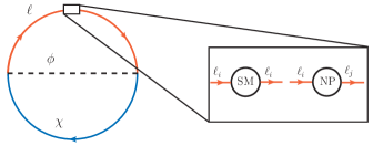
Figure 2: The 2PI effective action $\Gamma_{2}$ at two-loop order in the CTP formalism. The propagators in the closed loop are in their full forms. In particular, the resummed lepton propagator includes 1PI diagrams from the SM flavor-conserving gauge and Yukawa interactions, and the NP flavor-violating Yukawa interactions. The self-energy amplitudes of $\chi$ are obtained by opening the $\chi$ line, corresponding to the functional derivative of $\Gamma_{2}$: $i\not{\Sigma}_{\chi}^{ab}=ab\,\delta\Gamma_{2}/\delta\not{S}_{\chi}^{ba}$ with thermal indices $a,b=\pm$.

In a spatially homogeneous background, the KB equation of $\chi_{1}$ can be formally written as SM

$$\frac{d(sY_{\chi_{1}})}{dt}=\mathcal{W}+\mathcal{S}_{\rm CP}\,,$$ (4)

where $\mathcal{W}$ denotes the washout rate and $\mathcal{S}_{\rm CP}$ the CP-violating source

$$\mathcal{S}_{\rm CP}=\frac{1}{2}\int\frac{d^{4}p}{(2\pi)^{4}}\text{Tr}\left[i\not{\Sigma}_{\chi_{1}}^{>}i\not{S}_{\chi_{1}}^{<}-i\not{\Sigma}_{\chi_{1}}^{<}i\not{S}_{\chi_{1}}^{>}\right],$$ (5)

with $-i\not{\Sigma}_{\chi_{1}}^{>,<}$ the self-energy amplitudes of $\chi_{1}$, $i\not{S}_{\chi_{1}}^{<,>}$ the Wightman functions and $\rm Tr$ the Dirac trace. In full thermal equilibrium, the Kubo–Martin–Schwinger (KMS) relations hold: $\not{\Sigma}_{\chi_{1}}^{>}(p)=-e^{p_{0}/T}\not{\Sigma}_{\chi_{1}}^{<}(p),\not{S}_{\chi_{1}}^{>}(p)=-e^{p_{0}/T}\not{S}^{<}_{\chi_{1}}(p)$, such that the source term vanishes and no $\chi_{1}$ asymmetry will be generated. The leading contribution to the washout rate $\mathcal{W}$ is determined by the one-loop self-energy diagram of $\chi_{1}$ without resummation, while the forbidden CP asymmetry of $\chi_{1}$ comes from the middle diagram of Fig. 1, with the resummed lepton propagators and the inner loop shown in Fig. 2. The calculation of $\mathcal{S}_{\rm CP}$ constitutes one of the main difficulties in the KB equation, but we find that it can be greatly simplified after exploiting the integral symmetries and reasonable approximations. The final result succinctly reads SM

$$\mathcal{S}_{\rm CP} =\frac{\text{Im}(y^{\prime 4})m_{\phi}^{4}}{256\pi^{4}(\tilde{m}_{j}^{2}-\tilde{m}_{i}^{2})}\mathcal{I}\,,$$ (6)

where $\text{Im}(y^{\prime 4})\equiv\text{Im}[y^{\prime}_{i1}y^{\prime*}_{j1}y^{\prime*}_{i2}y^{\prime}_{j2}]$ and $i\neq j$ are summed over three lepton flavors. $\mathcal{I}$ represents the statistic nature of the forbidden CP asymmetry:

$$\mathcal{I} =\int_{0}^{\infty}\frac{dp_{\ell}}{p_{\ell}}\int^{\infty}_{p_{\ell}+m_{\phi}^{2}/(4p_{\ell})}dE_{\phi}\int^{\infty}_{p_{\ell}+m_{\phi}^{2}/(4p_{\ell})}dE^{\prime}_{\phi}$$

$$\times f_{\phi}^{\rm eq}(E_{\phi})\delta f_{\phi}(E^{\prime}_{\phi})\left[f^{\rm eq}_{\chi_{2}}(E_{\phi}^{\prime}-p_{\ell})+f^{\rm eq}_{\ell}(p_{\ell})-1\right],$$ (7)

where $\delta f_{\phi}\equiv f_{\phi}-f_{\phi}^{\rm eq}$, $E_{\phi}^{(\prime)}$ is the scalar energy in the outer (inner) loop, and we used the thermal distribution functions for $\chi_{2},\ell$.

From Eq. (Resonant Forbidden CP Asymmetry from Soft Leptons), we can infer the underlying nature of the forbidden CP asymmetry from the dependence of $\delta f_{\phi}(E^{\prime}_{\phi})$: the generation rate of forbidden CP asymmetries must be scaled with the distribution functions of the inner loop particles. This is understood if we omit the statistics of $\phi$ in the inner loop: $f_{\phi}^{(\rm eq)}(E^{\prime}_{\phi})=0$, which gives rise to $\mathcal{S}_{\rm CP}=0$. Thus, we quantitatively confirm the expectation outlined at the beginning of this Letter that the probability of the forbidden CP asymmetry is proportional to distribution functions of the inner onshell particles. Note that $\mathcal{S}_{\rm CP}$ exhibits a scaling similar to Eq. (1), and the complex Yukawa couplings at quartic order provide the necessary CP-violating phase.

Using Eq. (2), we can estimate the CP-violating source at $T\simeq m_{\phi}$ as $\mathcal{S}_{\rm CP}\propto\text{Im}(y^{\prime 4})/(y_{j}^{2}-y_{i}^{2})$, where the flavor-universal gauge couplings are canceled and the survived charged-lepton Yukawa couplings cause an enhancement. Note that thermal widths of leptons are not included in Eq. (6). Actually, the quasiparticle nature of a thermal lepton flavor $i$ not only has a flavor-dependent pole: $p_{0}^{2}-|\vec{p}|^{2}\approx 2\tilde{m}_{i}^{2}$ Weldon:1982bn ; Kiessig:2010pr ; Li:2023ewv , but also predicts a thermal width at $\mathcal{O}(g^{4})$ SM . Since $g^{4}\gg y_{i}^{2}$ for all lepton flavors, inserting the width to the denominator of Eq. (6) seems to reduce the strong resonance.

However, the insertion is not a consistent treatment under finite-temperature perturbation theory. The underlying reason is that the leading thermal widths are at the same order in gauge couplings for all lepton flavors, which dictates that the thermal widths at a given order should be kept or neglected universally for all leptons. A demonstration is presented in SM with the Cauchy’s residue theorem. Here we consider a simpler way to see this. The scaling $1/(y_{j}^{2}-y_{i}^{2})$ comes from the product $S^{R}_{i}\times S^{<}_{j}$ in $\mathcal{S}_{\rm CP}$, with $S^{R}_{i},S^{<}_{j}$ the resummed retarded propagator and the Wightman function

$${S}^{R}_{i}\propto\frac{1}{\text{Re}\Delta_{i}+i\text{Im}\Delta_{i}},~{}{S}^{<}_{j}\propto\frac{\text{Im}\Delta_{j}}{(\text{Re}\Delta_{j})^{2}+(\text{Im}\Delta_{j})^{2}}\,.$$ (8)

The real part $\text{Re}\Delta$ determines the modified dispersion relation while the imaginary part $\text{Im}\Delta$ represents a finite width. At the pole $p^{2}\approx 2\tilde{m}_{j}^{2}$, the leading-order dependence of both $\text{Im}\Delta_{i}$ and $\text{Im}\Delta_{j}$ on the flavor-universal gauge couplings is at $\mathcal{O}(g^{4})$, so that $S^{R}_{i}(p)\times S^{<}_{j}(p)\propto(\tilde{m}_{j}^{2}-\tilde{m}_{i}^{2})^{-1}\times\delta(p^{2}-2\tilde{m}_{j}^{2})$ holds up to $\mathcal{O}(g^{2})$. This is different from vacuum mass degeneracy invoked in resonant leptogenesis, where two neutrino/scalar flavors having vacuum mass degeneracy do not have guaranteed decay widths at the same order of couplings. Going to $\mathcal{O}(g^{4})$, we may write $S^{<}_{j}(p)\propto\delta[p^{2}-2\tilde{m}_{j}^{2}-g^{4}q_{1}-ig^{4}q_{2}]$, with $q_{1,2}$ the functions of momentum and temperature SM . It is straightforward to check $S^{R}_{i}(p)\times S^{<}_{j}(p)\propto(\tilde{m}_{j}^{2}-\tilde{m}_{i}^{2})^{-1}\times\delta(p^{2}-2\tilde{m}_{j}^{2}-g^{4}q_{1}-ig^{4}q_{2})$, where the $\mathcal{O}(g^{4})$ terms from $S^{R}_{i}$ and $S^{<}_{j}$ cancel in the denominator. We can further go to higher orders of gauge couplings and repeat the above perturbation analysis. Generically, all the flavor-universal terms will be canceled in the product $S^{R}_{i}\times S^{<}_{j}$, leaving $g^{2}y_{i}^{2}$ and $g^{2}y_{j}^{2}$ as the next-to-leading-order flavor-dependent terms in the denominator of Eq. (6).

To proceed with the numerical computation of Eq. (4), we will work in the weak washout regime, where $\chi_{1}$ is not initially present in the SM plasma and $\mathcal{W}$ can be neglected. The weak washout regime can be characterized by the ratio of the decay width to Hubble expansion rate $R_{w}\equiv\Gamma_{\phi\to\ell+\chi_{1}}/H$ evaluated at $T=m_{\phi}$. Numerically, we apply Buchmuller:2004nz

$$R_{w}=\frac{y_{1}^{\prime 2}m^{*}_{\rm Pl}}{16\pi m_{\phi}}\lesssim 1\,,$$ (9)

where $y_{j}^{\prime 2}\equiv\sum_{i}|y^{\prime}_{ij}|^{2}$, and $m^{*}_{\rm Pl}\approx 7.11\times 10^{17}$ GeV is a reduced Planck mass. In this regime, Eq. (4) reduces to

$$\frac{\partial Y_{\chi_{1}}}{\partial T}=-\frac{\mathcal{S}_{\rm CP}}{sHT}\,,$$ (10)

after the replacement $d/dt\to\partial/\partial t+3HsY_{\chi_{1}}$. The source term depends on the scalar distribution function $f_{\phi}$ that should be solved first. To this aim, we use a Yukawa coupling $y^{\prime}_{2}=0.05$ to simplify the scalar evolution via $\phi\leftrightharpoons\ell+\chi_{2}$, which indicates that the decay/inverse decay will dominate the gauge-scalar scattering at the leptogenesis epoch. The leading scalar KB equation gives SM

$$\frac{df_{\phi}}{dt}=-\delta f_{\phi}\frac{|y^{\prime}_{2}|^{2}m_{\phi}^{2}T}{8\pi E_{\phi}p_{\phi}}\ln\left(\frac{\cosh p_{1}}{\cosh p_{2}}\right)\,,$$ (11)

where $d/dt=\partial/\partial t-Hp_{\phi}\partial/\partial p_{\phi}$, $p_{1,2}=(E_{\phi}\pm p_{\phi})/(4T)$ and $p_{\phi}\equiv|\vec{p}_{\phi}|$. Substituting the solution $f_{\phi}$ into $\mathcal{S}_{\rm CP}$ with an initial condition $f_{\phi}=f_{\phi}^{\rm eq}$ set at $z_{0}\equiv m_{\phi}/T_{0}=10^{-5}$, we show in Fig. 3 the evolution of $Y_{\chi_{1}}$, with the maximal enhancement from the muon flavor, i.e., $\mathcal{S}_{\rm CP}(j=2,i=1)$ and a maximal CP-violating Yukawa combination: $\text{Im}(y^{\prime 4})=-y^{\prime 2}_{1}y^{\prime 2}_{2}$.

We see from Fig. 3 that the scalar as low as 3.5 TeV is feasible to generate the baryon asymmetry via the secluded flavor effect (3). Fixing $R_{w}=1$, a heavier scalar $\phi$ will enhance the prefactor of Eq. (6) and hence the secluded asymmetry $Y_{\chi_{1}}$. Fixing $m_{\phi}$, $Y_{\chi_{1}}$ will increase as $R_{w}$ goes to higher values. For $R_{w}\gg 1$, however, leptogenesis will enter the strong washout regime, where $f_{\chi_{1}},f_{\bar{\chi}_{1}}$ and $\mathcal{W}$ cannot be neglected. In this regime, we expect that the resonant forbidden CP asymmetry still works with a larger Yukawa coupling $y^{\prime}_{1}$, depending on the competition between $\mathcal{W}$ and $\mathcal{S}_{\rm CP}$.

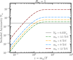
Figure 3: The secluded $\chi_{1}$ asymmetry with the maximally resonant enhancement: $\mathcal{S}_{\rm CP}(j=2,i=1)$ and $\text{Im}[y^{\prime}_{11}y^{\prime*}_{21}y^{\prime*}_{12}y^{\prime}_{22}]\approx-y^{\prime 2}_{1}y^{\prime 2}_{2}$. The horizontal line corresponds to the observed baryon asymmetry that would be created via the secluded flavor effect.

Working regimes.— The resonant enhancement relies on the lepton thermal mass given by Eq. (2), which assumes all charged-lepton Yukawa interactions are in thermal equilibrium. Particularly, the maximal enhancement requires the muon Yukawa interaction should be stronger than the Hubble expansion rate, which occurs at $T<10^{9}$ GeV. Therefore, the resonant forbidden CP asymmetry favors low-scale leptogenesis.

In deriving Eq. (6), we did not include the NP contribution to $\tilde{m}^{2}$. This is reasonable since Eq. (2) is derived with thermal and massless SM particles, while including the $\phi$-$\chi_{2}$ coupling in Eq. (2) depends on the nonthermal scalar distribution $f_{\phi}$ and introduce an exponential scaling $e^{-m_{\phi}/T}$. As leptogenesis culminates at $T<m_{\phi}$, the NP contribution to $\tilde{m}^{2}$ would be exponentially suppressed. Note that if the NP contribution happens to be comparable to the $y_{i}$ term, we can infer from Eq. (6) that $Y_{\chi_{1}}\propto\mathcal{O}(y^{\prime 2})$ instead of the more conventional situation $Y_{\chi_{1}}\propto\mathcal{O}(y^{\prime 4})$. This is an interesting possibility but it requires solving the time evolution of $\tilde{m}^{2}$ due to the $f_{\phi}$ dependence.

The exemplary scalar has gauge interaction, e.g., via contact scattering with $SU(2)_{L}$ gauge bosons $W_{\mu}^{i}$: $\phi+\phi^{\dagger}\leftrightharpoons W_{\mu}^{i}+W^{\mu i}$. The scalar via such gauge interaction must freeze out before sphaleron decoupling at $T_{\rm sph}\approx 132$ GeV DOnofrio:2014rug . Otherwise the scalar would still be in thermal equilibrium and Eq. (6) would vanish. Given that the weak interaction typically implies a freeze-out temperature $T_{\rm fo}\approx m_{\phi}/25$ Kolb:1990vq , we obtain a lower mass bound on the nonthermal scalar through $T_{\rm fo}>T_{\rm sph}$, leading to

$$m_{\phi}\gtrsim 3.3~{}\rm TeV\,.$$ (12)

Note that, however, the scalar doublet being in thermal equilibrium can still work to generate a nonzero forbidden CP asymmetry if the nonthermal condition comes from $\chi_{2}$ SM . Besides, the exemplary scalar decay shown in this Letter can also be switched to $\chi_{1}$ decay if $m_{\chi_{1}}>m_{\phi}$. For both cases, Eq. (12) does not apply. Therefore, low-scale leptogenesis from the forbidden CP asymmetry allows a decaying $\phi$ at the electroweak scale and much lighter fermion products $\chi$, making production attainable from low-energy experiments such as LHC and future Higgs factories. The present example also demonstrates that mixing from scalars is not necessary to induce CP asymmetry in scalar decay. Therefore, it allows minimal model buildings, e.g., in Dirac leptogenesis Dick:1999je ; Murayama:2002je and seesaw type-II leptogenesis Ma:1998dx .

The main results in this Letter exploit the maximal role of resummed leptons in generating CP asymmetries, but we do not intend to specify $\phi,\chi$. Actually, the mechanism works for a wide class of particles $\phi,\chi$. For example, the particle set $(\phi,\chi)$ may be identified as (scalar triplet, SM charged leptons) or (scalar doublet, sterile neutrinos). $(\phi,\chi)$ could also be specified as dark matter candidates, thereby featuring a novel cogenesis mechanism for dark matter and the BAU.

When $(\phi,\chi)$ is identified as the SM Higgs and Majorana neutrinos, it reduces to the prototype of the canonical type-I seesaw leptogenesis Fukugita:1986hr ; Luty:1992un ; Covi:1996wh . The contribution from the resonant forbidden CP asymmetry may be noticeable in low-scale type-I leptogenesis, but the $\chi_{1}$ asymmetry computed here cannot be directly applied if the lepton number is violently broken in the leptogenesis epoch. In this case, one should build upon the mixed KB kinetic equations, which goes beyond the unmixed KB equation used in this Letter but deserves full considerations.

Nevertheless, the resonantly enhanced $\chi_{1}$ asymmetry is valid if the lepton-number breaking effect is negligible at the leptogenesis epoch, which is the case for pseudo-Dirac neutrinos Wyler:1982dd in low-scale seesaw frameworks Mohapatra:1986bd ; Branco:1988ex ; Shaposhnikov:2006nn ; Kersten:2007vk ; Abada:2017ieq , or for relativistic Majorana neutrinos having approximately conserved helicity numbers at leptogenesis temperatures Akhmedov:1998qx ; Abada:2018oly . In particular, the BAU can be generated by SM Higgs decay to GeV-scale Majorana neutrinos. It was pointed out that a minimal neutrino mass degeneracy at level of $10^{-5}$ is needed to enhance the CP asymmetry in SM Higgs decay Hambye:2016sby . However, the thermal mass degeneracy from resummed leptons implies that an enhancement larger than $10^{5}$ is feasible without neutrino mass degeneracy.

In conclusion, SM leptons at high temperatures can give rise to a large plasma-induced (forbidden in vacuum) CP asymmetry, which will work as an irreducible contribution to low-scale leptogenesis. The resonant forbidden CP asymmetry also provides a new mechanism for leptogenesis where vacuum cuts or vacuum mass degeneracy are absent in the NP sector, allowing minimal and testable model exploitation.

Acknowledgements.— We would like to thank Yushi Mura for frequent discussions during this project and Ke-Pan Xie for useful comments. This project is supported by JSPS Grant-in-Aid for JSPS Research Fellows No. 24KF0060. SK is also supported in part by Grants-in-Aid for Scientific Research (KAKENHI) Nos. 23K17691 and 20H00160.

Supplemental Material

Resonant Forbidden CP Asymmetry from Soft Leptons

Shinya Kanemura and Shao-Ping Li

Appendix A CTP formalism and HTL resummation

In the Closed-Timed-Path (CTP) formalism, free propagators in a spatially homogeneous and close-to-equilibrium plasma can be formulated by

$$i\not{S}^{+-}(p) \equiv i\not{S}^{<}(p)=-2\pi\delta(p^{2}-m^{2})(\not{p}+m)\left[\theta(p_{0})f(p_{0})-\theta(-p_{0})(1-\bar{f}(-p_{0}))\right],$$ (13)

$$i\not{S}^{-+}(p) \equiv i\not{S}^{>}(p)=-2\pi\delta(p^{2}-m^{2})(\not{p}+m)\left[-\theta(p_{0})(1-f(p_{0})+\theta(-p_{0})\bar{f}(-p_{0})\right],$$ (14)

$$i\not{S}^{++}(p) \equiv i\not{S}^{T}(p)=\frac{i(\not{p}+m)}{p^{2}-m^{2}+i\epsilon}-2\pi\delta(p^{2}-m^{2})(\not{p}+m)\left[\theta(p_{0})f(p_{0})+\theta(-p_{0})\bar{f}(-p_{0})\right],$$ (15)

$$i\not{S}^{--}(p) \equiv i\not{S}^{\bar{T}}(p)=-\frac{i(\not{p}+m)}{p^{2}-m^{2}-i\epsilon}-2\pi\delta(p^{2}-m^{2})(\not{p}+m)\left[\theta(p_{0})f(p_{0})+\theta(-p_{0})\bar{f}(-p_{0})\right],$$ (16)

for massive Dirac fermions, and

$$iG^{+-}(p) \equiv iG^{<}(p)=2\pi\delta(p^{2}-m^{2})\left[\theta(p_{0})f(p_{0})+\theta(-p_{0})(1+\bar{f}(-p_{0}))\right],$$ (17)

$$iG^{-+}(p) \equiv iG^{>}(p)=2\pi\delta(p^{2}-m^{2})\left[\theta(p_{0})(1+f(p_{0}))+\theta(-p_{0})\bar{f}(-p_{0})\right],$$ (18)

$$iG^{++}(p) \equiv iG^{T}(p)=\frac{i}{p^{2}-m^{2}+i\epsilon}+2\pi\delta(p^{2}-m^{2})\left[\theta(p_{0})f(p_{0})+\theta(-p_{0})\bar{f}(-p_{0})\right],$$ (19)

$$iG^{--}(p) \equiv iG^{\bar{T}}(p)=-\frac{i}{p^{2}-m^{2}-i\epsilon}+2\pi\delta(p^{2}-m^{2})\left[\theta(p_{0})f(p_{0})+\theta(-p_{0})\bar{f}(-p_{0})\right],$$ (20)

for massive scalars. Here, $\pm$ denote the thermal indices, $\lessgtr$ represent the Wightman functions and $T(\bar{T})$ the (anti) time-ordered propagators. $f,\bar{f}$ are the distribution functions of particles and antiparticles with $\bar{f}(p_{0})=1-f(-p_{0})$ for fermions and $\bar{f}(p_{0})=-1-f(-p_{0})$ for scalars Prokopec:2003pj ; Prokopec:2004ic . Note that for SM lepton doublets being left-handed and massless, we should insert the chirality projection operators $P_{L,R}\equiv(1\mp\gamma_{5})/2$ into $\not{S}^{ab}$ via $(\not{p}+m)\to P_{L}\not{p}P_{R}$. In thermal equilibrium, we have

$$f(p_{0})=\bar{f}(p_{0})=\frac{1}{e^{p_{0}/T}\pm 1}\,$$ (21)

for fermions ($+$) and bosons ($-$). Besides, the Kubo–Martin–Schwinger (KMS) relations hold $\not{S}^{>}(p)=-e^{p_{0}/T}\not{S}^{<},G^{>}(p)=e^{p_{0}/T}G^{<}(p)$.

The resummed scalar propagator concerned in this Letter can be described by adding the thermal mass effect to the vacuum mass, which is nevertheless subdominant. For SM singlets $\chi_{1,2}$, the thermal mass effects arise from the small Yukawa couplings $y^{\prime}$ and we also treat them as subdominant thermal corrections to vacuum masses. To derive the resummed lepton propagators, we use the approximation that leptons are in thermal equilibrium during the leptogenesis epoch. The resummed Wightman functions are written as

$$\not{S}^{<}(p) =-f(p_{0})\left(\not{S}^{R}-\not{S}^{A}\right),$$ (22)

$$\not{{S}}^{>}(p) =\left[1-f(p_{0})\right]\left(\not{{S}}^{R}-\not{{S}}^{A}\right),$$ (23)

where $\not{{S}}^{R}$ and $\not{{S}}^{A}$ are the resummed retarded and advanced propagators satisfying

$$\not{{S}}^{T}-\not{{S}}^{\bar{T}}=\not{{S}}^{R}+\not{{S}}^{A},\quad\not{{S}}^{>}-\not{{S}}^{<}=\not{{S}}^{R}-\not{{S}}^{A}\,.$$ (24)

The resummed retarded propagator is generally written as Weldon:1982bn ; Li:2023ewv

$$\not{{S}}^{R}(p) =P_{L}\frac{(1+a)\not{p}+b\not{u}}{\left[(1+a)p_{0}+b\right]^{2}-\left[(1+a)|\vec{p}|\right]^{2}}P_{R}$$ (25)

$$\equiv\sum_{\pm}\frac{1}{\text{Re}\Delta_{\pm}+i\text{Im}\Delta_{\pm}}{P}_{\pm}\,,$$ (26)

where $u_{\mu}$ is the four-velocity of the plasma normalized by $u_{\mu}u^{\mu}=1$ with $u_{\mu}=(1,0,0,0)$ in the rest frame. Note that we have omitted the $i\text{sign}(p_{0})\epsilon$ prescription for resummed propagators. The modified dispersion relation and thermal width are determined by the real and imaginary parts, respectively:

$$\text{Re}\Delta_{\pm}(p) \equiv(1+\text{Re}a)(p_{0}\pm|\vec{p}|)+\text{Re}b\,,$$ (27)

$$\text{Im}\Delta_{\pm}(p) \equiv\text{Im}a(p_{0}\pm|\vec{p}|)+\text{Im}b\,,$$ (28)

and $P_{\pm}$ denotes the decomposition of helicity eigenstates Braaten:1990wp

$$P_{\pm}\equiv P_{L}\frac{\gamma^{0}\pm\vec{e}_{p}\cdot\vec{\gamma}}{2}P_{R}\,,$$ (29)

with $\vec{e}_{p}\equiv\vec{p}/|\vec{p}|$. The resummed advanced propagator can be obtained via $a,b\to a^{*},b^{*}$, giving rise to

$$\not{{S}}^{R}-\not{{S}}^{A}=\sum_{\pm}\frac{-2i\text{Im}\Delta_{\pm}}{(\text{Re}\Delta_{\pm})^{2}+(\text{Im}\Delta_{\pm})^{2}}P_{\pm}\,.$$ (30)

The real coefficients $\text{Re}a,\text{Re}b$ are well known in the HTL approximation Weldon:1982bn ; Li:2023ewv

$$\text{Re}a_{i} =\frac{\tilde{m}^{2}_{i}}{|\vec{p}|^{2}}\left[1+\frac{p_{0}}{2|\vec{p}|}\ln\left(\frac{p_{0}-|\vec{p}|}{p_{0}+|\vec{p}|}\right)\right],$$ (31)

$$\text{Re}b_{i} =-\frac{\tilde{m}^{2}_{i}}{|\vec{p}|}\left[\frac{p_{0}}{|\vec{p}|}-\frac{1}{2}\left(1-\frac{p_{0}^{2}}{|\vec{p}|^{2}}\right)\ln\left(\frac{p_{0}-|\vec{p}|}{p_{0}+|\vec{p}|}\right)\right]\,,$$ (32)

with the properties $\text{Re}a_{i}(p_{0})=\text{Re}a_{i}(-p_{0}),\text{Re}b_{i}(p_{0})=-\text{Re}b_{i}(-p_{0})$, and the thermal masses of leptons:

$$\tilde{m}_{i}^{2}=\left(\frac{3}{32}g_{2}^{2}+\frac{1}{32}g_{1}^{2}+\frac{1}{16}y_{i}^{2}\right)T^{2}\,.$$ (33)

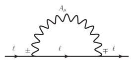
Figure 4: Contributions to thermal widths of leptons from gauge interactions, where $A_{\mu}=W_{\mu},B_{\mu}$ denote gauge $SU(2)_{L}$ and $U(1)_{Y}$ bosons and $\pm$ the thermal indices.

In the zero-width approximation, $\text{Im}\Delta_{\pm}\to 0$, the pole of both $\not{{S}}^{R}$ and $\not{{S}}^{R}-\not{{S}}^{A}$ (hence $\not{{S}}^{<,>}$) is determined by $\text{Re}\Delta_{\pm}=0$, which gives

$$p_{0}=\mp\left[|\vec{p}|+\frac{\tilde{m}^{2}}{|\vec{p}|}-\frac{\tilde{m}^{4}}{2|\vec{p}|^{3}}\log\left(\frac{2|\vec{p}|^{2}}{\tilde{m}^{2}}\right)+\mathcal{O}(\tilde{m}^{6})\right].$$ (34)

At $\mathcal{O}(\tilde{m}^{2})$, the dispersion relations can be well approximated by two modes: $p_{0}^{2}-|\vec{p}|^{2}\approx 0$ and $p_{0}^{2}-|\vec{p}|^{2}\approx 2\tilde{m}^{2}$ Kiessig:2010pr ; Drewes:2013iaa ; Li:2023ewv . The first mode is flavor blind and will not give rise to the forbidden CP asymmetry that is lepton-flavor dependent. Neglecting $\mathcal{O}(g^{4})$ contributions to the pole, we would arrive at the onshell propagation from the second mode:

$$i\not{{S}}^{R}_{i}(p)\Big{|}_{\rm onshell} \approx\pi\text{sign}(p_{0})\delta(p^{2}-2\tilde{m}_{i}^{2})P_{L}\not{p}P_{R}\,,$$ (35)

$$i\not{{S}}_{i}^{<}(p)\Big{|}_{\rm onshell} \approx-2\pi\text{sign}(p_{0})f(p_{0})\delta(p^{2}-2\tilde{m}_{i}^{2})P_{L}\not{p}P_{R}\,,$$ (36)

$$i\not{{S}}_{i}^{>}(p)\Big{|}_{\rm onshell} \approx 2\pi\text{sign}(p_{0})\left[1-f(p_{0})\right]\delta(p^{2}-2\tilde{m}_{i}^{2})P_{L}\not{p}P_{R}\,,$$ (37)

where the resummed Wightman functions have the same form as in the free case.

To see the consequence of including $\text{Im}\Delta_{\pm}$ at higher orders of gauge couplings, which is important to check the stability of the resonant forbidden CP asymmetry, we next go beyond the zero-width approximation by including the finite width from $\text{Im}\Delta_{\pm}$ perturbatively. To this aim, we first calculate the imaginary coefficients $\text{Im}a,\text{Im}b$. Consider the leading-order contribution from the gauge 1PI diagrams shown in Fig. 4. The imaginary part of the retarded amplitude for the SM leptons can be calculated via

$$\text{Im}\Sigma^{R}=-\frac{i}{2}\left(\Sigma^{>}-\Sigma^{<}\right)\,,$$ (38)

and the imaginary coefficients $\text{Im}a,\text{Im}b$ read

$$\text{Im}a =\frac{1}{2|\vec{p}|^{2}}\left(\text{Tr}[\not{p}\text{Im}\Sigma^{R}(p)]-p_{0}\text{Tr}[\not{u}\text{Im}\Sigma^{R}(p)]\right),$$ (39)

$$\text{Im}b =-\frac{1}{2|\vec{p}|^{2}}\left(p_{0}\text{Tr}[\not{p}\text{Im}\Sigma^{R}(p)]-p^{2}\text{Tr}[\not{u}\text{Im}\Sigma^{R}(p)]\right).$$ (40)

A straightforward calculation of Fig. 4 at $\text{Re}\Delta_{\pm}=0$ gives

$$\text{Im}\Delta_{\pm}=\kappa g^{2}\frac{\tilde{m}^{2}}{|\vec{p}|}\,,$$ (41)

where $g^{2}\equiv 3g_{2}^{2}+g_{1}^{2}$ includes the contributions from $SU(2)_{L}$ and $U(1)_{Y}$ gauge bosons, and for simplicity we have taken $T=|\vec{p}|$ to turn the loop integration into a numerical coefficient $\kappa\approx 4\times 10^{-3}$. We see that the leading dependence of $\text{Im}\Delta_{\pm}$ on gauge couplings is at $\mathcal{O}(g^{4})$, which is indeed a higher-order effect for Eqs. (35)-(37).

As will be shown in Appendix C, the product ${S}_{i}^{R}\times{S}^{<}_{j}$ contributes to the resonance. Besides, the kinetics shown in Appendix C selects one of the poles from Eq. (34), so only the $P_{+}\times P_{+}$ or $P_{-}\times P_{-}$ component in the product ${S}_{i}^{R}\times{S}^{<}_{j}$ will contribute to the resonance. Here, the unslashed propagators denote the c-numbers from the slashed propagators, e.g., the $P_{+}$ component of $S^{R}$ is defined as: $[S^{R}]_{+}\equiv 1/(\text{Re}\Delta_{+}+i\text{Im}\Delta_{+})$. Let us consider the $P_{+}\times P_{+}$ component at $\mathcal{O}(g^{2})$, though the analysis for the $P_{-}\times P_{-}$ component is essentially the same. Using Eq. (36) and (26), and factoring out the distribution functions, we arrive at

$$\left[S_{i}^{R}(p)\times S^{<}_{j}(p)\right]_{++}=2\pi i\frac{\delta(\text{Re}\Delta_{+j})}{\text{Re}\Delta_{+i}}=2\pi i\frac{|\vec{p}|}{\tilde{m}_{i}^{2}-\tilde{m}_{j}^{2}}\delta(p_{0}+\omega_{j})\,,$$ (42)

where $\omega_{j}=(|\vec{p}|^{2}+2\tilde{m}_{j}^{2})^{1/2}$ corresponds to the pole given in Eq. (34) up to $\mathcal{O}(g^{2})$. Equation (42) demonstrates the origin of the resonant enhancement at $\mathcal{O}(g^{2})$.

When including $\text{Im}\Delta_{\pm}$ at $\mathcal{O}(g^{4})$, we can analyze the resonance by using the Cauchy’s residue theorem. The $P_{+}\times P_{+}$ component of the $S_{i}^{R}\times S^{<}_{j}$ product now has a pole from $[S^{<}_{j}]_{+}$:

$$p_{0}=-\left[|\vec{p}|+\frac{\tilde{m}_{j}^{2}}{p}-\frac{\tilde{m}_{j}^{4}}{2|\vec{p}|^{3}}\log\left(\frac{2|\vec{p}|^{2}}{\tilde{m}_{j}^{2}}\right)+i\kappa g^{2}\frac{\tilde{m}_{j}^{2}}{|\vec{p}|}\right].$$ (43)

Choosing the lower half-plane contour that encloses the above pole would give rise to

$$\left[{S}_{i}^{R}(p)\times{S}^{<}_{j}(p)\right]_{++}\xrightarrow{\oint_{c}}2\pi i\frac{|\vec{p}|}{\tilde{m}_{i}^{2}-\tilde{m}_{j}^{2}+i\kappa g^{2}(\tilde{m}_{i}^{2}-\tilde{m}_{j}^{2})}\,.$$ (44)

Here $\xrightarrow{\oint_{c}}$ indicates that the right-hand side is the result that would be obtained after performing the contour integration, with a factor of $-2\pi i$ from the residue theorem. We see that the next-to-leading-order contribution beyond $\tilde{m}_{i}^{2}-\tilde{m}_{j}^{2}$ is $\kappa g^{2}(\tilde{m}_{i}^{2}-\tilde{m}_{j}^{2})$, which is at $\mathcal{O}(g^{2}y^{2})$. Given $\kappa g^{2}(\tilde{m}_{i}^{2}-\tilde{m}_{j}^{2})\ll\tilde{m}_{i}^{2}-\tilde{m}_{j}^{2}$, the result shown in Eq. (44) will approximately reduce to that in Eq. (42) after the full momentum integration. Therefore, including the $\mathcal{O}(g^{4})$ contribution both in the dispersion relation and thermal width will not destroy the resonance, since the dependence on the flavor-universal gauge couplings is canceled. In fact, going to $\mathcal{O}(g^{n>4})$, one can repeat the above perturbative analysis, and the gauge-coupling dependence will be canceled in the denominator order by order, leaving terms involving the mixed couplings $g^{a}y^{b}$ with $a+b=n$.

Note that there is another pole in the $P_{+}\times P_{+}$ component of ${S}_{i}^{R}\times{S}^{<}_{j}$, which comes from $[S^{R}_{i}]_{+}$. However, the contribution from this pole does not exhibit a resonance enhanced by $\mathcal{O}(y^{-2})$. One can check this by applying the residue theorem with the pole of $[S^{R}_{i}]_{+}$, which is given by Eq. (43) with the replacement $\tilde{m}_{j}\to\tilde{m}_{i}$.

The above derivation shows that we should take the thermal widths of lepton flavors in a way consistent with the HTL perturbative expansion. Using the zero-width approximation for the Wightman functions but inserting the thermal width in the retarded propagator is not a consistent treatment, since the former is not valid when keeping the $\mathcal{O}(g^{4})$ terms. The identical dependence on gauge couplings of different lepton flavors ensures that the resonance from $1/(\tilde{m}_{i}^{2}-\tilde{m}_{j}^{2})$ is stable under higher-order gauge corrections to lepton dispersion relations and thermal widths.

Appendix B Kadanoff-Baym equations

The KB equation (4) is derived from the full kinetic equation, which in Wigner space is given by Prokopec:2003pj

$$(\not{p}+\frac{i}{2}\not{\partial}_{x}-m_{\chi_{1}}e^{-i\overleftarrow{\partial_{x}}\cdot\partial_{p}/2})\not{S}_{\chi_{1}}^{<,>}-e^{-i\diamond/2}\{\not{\Sigma}_{h}\}\{\not{S}_{\chi_{1}}^{<,>}\}-e^{-i\diamond/2}\{\not{\Sigma}_{\chi_{1}}^{<,>}\}\{\not{S}_{h}\}=\mathcal{C}_{\chi_{1}}\,,$$ (45)

where $\partial_{x}\equiv\partial/\partial x,\partial_{p}\equiv\partial/\partial p$ are the spacetime and 4-momentum derivatives, and the symbol $\diamond$ denotes the so-called diamond operator with $\diamond\{A\}\{B\}=(\partial_{x}A)(\partial_{p}B)-(\partial_{p}A)(\partial_{x}B)$. The propagator $\not{S}_{h}$ and the self-energy amplitude $\not{\Sigma}_{h}$ can be written in terms of time and anti-time ordered quantities:

$$\not{S}_{h}\equiv\frac{1}{2}(\not{S}_{\chi_{1}}^{T}-\not{S}_{\chi_{1}}^{\bar{T}})\,,\quad\not{\Sigma}_{h}\equiv\frac{1}{2}(\not{\Sigma}_{\chi_{1}}^{T}-\not{\Sigma}_{\chi_{1}}^{\bar{T}})\,.$$ (46)

$\mathcal{C}_{\chi_{1}}$ is the collision term accounting for gain and loss rates of $\chi_{1}$:

$$\mathcal{C}_{\chi_{1}}=\frac{1}{2}e^{-i\diamond/2}\left(\{\not{\Sigma}_{\chi_{1}}^{>}\}\{\not{S}_{\chi_{1}}^{<}\}-\{\not{\Sigma}_{\chi_{1}}^{<}\}\{S_{\chi_{1}}^{>}\}\right).$$ (47)

At zeroth order of gradient expansion: $e^{-i\diamond/2}\approx 1$, the kinetic equation with a constant mass reduces to

$$(\not{p}+\frac{i}{2}\not{\partial}_{x}-\tilde{m}_{\chi_{1}})\not{S}_{\chi_{1}}^{<,>}-\not{\Sigma}_{\chi_{1}}^{<,>}\times\not{S}_{h}=\frac{1}{2}\left(\not{\Sigma}_{\chi_{1}}^{>}\times\not{S}_{\chi_{1}}^{<}-\not{\Sigma}_{\chi_{1}}^{<}\times\not{S}_{\chi_{1}}^{>}\right),$$ (48)

where $\tilde{m}_{\chi_{1}}\equiv m_{\chi_{1}}+\not{\Sigma}_{h}$ includes vacuum and finite-temperature self-energy corrections to the dispersion relation of $\chi_{1}$. In the KB ansatz followed by the onshell quasiparticle approximation, we have $(\not{p}-\tilde{m}_{\chi_{1}})\not{S}_{\chi_{1}}^{<,>}=\not{\Sigma}_{\chi_{1}}^{<,>}\times\not{S}_{h}\approx 0$. Therefore, the KB kinetic equation reduces to

$$\gamma^{0}\frac{d}{dt}(i\not{S}_{\chi_{1}}^{<,>})=(-i\not{\Sigma}_{\chi_{1}}^{>})(i\not{S}_{\chi_{1}}^{<})-(-i\not{\Sigma}_{\chi_{1}}^{<})(i\not{S}_{\chi_{1}}^{>})\,,$$ (49)

where $-i$ attached to $\not{\Sigma}^{<,>}$ highlights the convention for self-energy amplitudes. Using Eqs. (13)-(14) for $\not{S}_{\chi_{1}}^{<,>}$, taking the Dirac trace on both sides of the above equation, and integrating over $d^{4}p_{\chi_{1}}/(2\pi)^{4}$, we will arrive at Eq. (4).

Note that the KB ansatz with the quasiparticle approximation is consistent with the pole equation Prokopec:2003pj ; Berges:2004yj

$$(\not{p}+\frac{i}{2}\not{\partial}_{x}-m_{\chi_{1}}e^{-i\overleftarrow{\partial_{x}}\cdot\partial_{p}/2})\not{S}_{\chi_{1}}^{r,a}-e^{-i\diamond/2}\{\not{\Sigma}_{\chi_{1}}^{r,a}\}\{\not{S}_{\chi_{1}}^{r,a}\}=\bf{1}\,,$$ (50)

where

$$\not{S}_{\chi_{1}}^{r,a} =\frac{1}{2}\left[\not{S}_{\chi_{1}}^{T}-\not{S}_{\chi_{1}}^{\bar{T}}\pm\left(\not{S}_{\chi_{1}}^{>}-\not{S}_{\chi_{1}}^{<}\right)\right]=\not{S}_{h}\pm\frac{1}{2}\left(\not{S}_{\chi_{1}}^{>}-\not{S}_{\chi_{1}}^{<}\right),$$ (51)

$$\not{\Sigma}_{\chi_{1}}^{r,a} =\frac{1}{2}\left[\not{\Sigma}_{\chi_{1}}^{T}-\not{\Sigma}_{\chi_{1}}^{\bar{T}}\pm\left(\not{\Sigma}_{\chi_{1}}^{>}-\not{\Sigma}^{<}\right)\right]=\not{\Sigma}_{h}\pm\frac{1}{2}\left(\not{\Sigma}_{\chi_{1}}^{>}-\not{\Sigma}_{\chi_{1}}^{<}\right).$$ (52)

To check this, we take the difference $\not{S}^{r}-\not{S}^{a}$ via Eq. (50) in the onshell limit: $\not{S}_{h}=0$, which at zeroth order of gradient expansion gives rise to

$$(\not{p}+\frac{i}{2}\not{\partial}_{x}-\tilde{m}_{\chi_{1}})(\not{S}_{\chi_{1}}^{>}-\not{S}_{\chi_{1}}^{<})=0\,.$$ (53)

Further using the onshell limit $(\not{p}-\tilde{m}_{\chi_{1}})\not{S}_{\chi_{1}}^{<,>}=0$, we see that $\not{\partial}_{x}\not{S}_{\chi_{1}}^{>}=\not{\partial}_{x}\not{S}_{\chi_{1}}^{<}$, which is consistent with Eq. (49).

The full KB equation for scalar $\phi$ reads Prokopec:2003pj

$$e^{-i\diamond/2}\{p^{2}-\tilde{m}_{\phi}^{2}\}\{G_{\phi}^{<,>}\}-e^{-i\diamond/2}\{\Pi_{\phi}^{<,>}\}\{G_{h}\}=\frac{1}{2}e^{-i\diamond/2}\left(\{\Pi_{\phi}^{>}\}\{G_{\phi}^{<}\}-\{\Pi_{\phi}^{<}\}\{G_{\phi}^{>}\}\right),$$ (54)

where $\tilde{m}_{\phi}^{2}\equiv m_{\phi}^{2}+\Pi_{h}$ with

$$\Pi_{h}\equiv\frac{1}{2}(\Pi_{\phi}^{T}-\Pi_{\phi}^{\bar{T}})\,,\quad G_{h}=\frac{1}{2}(G_{\phi}^{T}-G_{\phi}^{\bar{T}})\,.$$ (55)

Similar to the fermion case, we have $(p^{2}-\tilde{m}_{\phi}^{2})G_{\phi}^{<,>}=\Pi_{\phi}^{<,>}\times G_{h}\approx 0$ in the onshell limit. Then expanding the gradient up to first order and neglecting the spacetime/4-momentum derivatives of loop amplitudes, we arrive at the Boltzmann equation given by Eq. (11), with the decay and inverse decay rates equivalent to what would be derived from the $S$-matrix formalism.

Note that the onshell approximation $(p^{2}-\tilde{m}_{\phi}^{2})G_{\phi}^{<,>}\approx 0$ is equivalent to $\Pi_{\phi}^{<,>}\times G_{h}\approx 0$ at zeroth order. To see this, we can derive the Hermitian part of Eq. (54),

$$e^{i\diamond/2}\{p^{2}-\tilde{m}_{\phi}^{2}\}\{G_{\phi}^{<,>}\}-e^{i\diamond/2}\{\Pi_{\phi}^{<,>}\}\{G_{h}\}=-\frac{1}{2}e^{i\diamond/2}\left(\{\Pi_{\phi}^{>}\}\{G_{\phi}^{<}\}-\{\Pi_{\phi}^{<}\}\{G_{\phi}^{>}\}\right),$$ (56)

where we have used the Hermitian conditions $(iG_{\phi}^{<,>})^{\dagger}=iG_{\phi}^{<,>}$, $(i\Pi_{\phi}^{<,>})^{\dagger}=i\Pi_{\phi}^{<,>}$ and $G_{h}^{\dagger}=G_{h}$. Then taking the sum of Eq. (54) and Eq. (56) and expanding to the first-order gradient, we arrive at the so-called constraint equation:

$$(p^{2}-\tilde{m}_{\phi}^{2})G_{\phi}^{<,>}+\frac{i}{4}\diamond\left(\{\Pi_{\phi}^{>}\}\{G_{\phi}^{<}\}-\{\Pi_{\phi}^{<}\}\{G_{\phi}^{>}\}\right)=\Pi_{\phi}^{<,>}\times G_{h}\,.$$ (57)

Therefore, the onshell limit $(p^{2}-\tilde{m}_{\phi}^{2})G_{\phi}^{<,>}=0$ indicates $\Pi_{\phi}^{<,>}\times G_{h}=0$ at zeroth order. Alternatively, the dissipative term $\Pi_{\phi}^{<,>}\times G_{h}$ is of the same order as the spacetime/4-momentum derivatives of loop amplitudes in the onshell limit, such that the kinetic equation for the scalar distribution function will reduce to the Boltzmann equation.

Appendix C CP-violating source

The discussion in Appendix A demonstrated that the thermal widths of resummed leptons are smaller than the thermal mass effects near the quasiparticle pole, and the resonance due to the thermal mass difference is insensitive to higher-order gauge coupling corrections. Given this, we will calculate the CP-violating source by neglecting contributions from $\mathcal{O}(g^{4})$.

The self-energy diagram of $\chi_{1}$ that contributes to the forbidden CP asymmetry is shown in Fig. 5, with the following amplitudes

$$i\not{\Sigma}_{\chi_{1}}^{<}(p) =2y^{\prime}_{i1}y_{j1}^{\prime*}\int\frac{d^{4}p_{\ell}}{(2\pi)^{4}}\frac{d^{4}p_{\phi}}{(2\pi)^{4}}(2\pi)^{4}\delta^{4}(p-p_{\ell}+p_{\phi})P_{L}i\not{{S}}^{<}_{\ell_{ij}}P_{R}iG_{\phi}^{>}\,,$$ (58)

$$i\not{\Sigma}_{\chi_{1}}^{>}(p) =2y^{\prime}_{i1}y^{\prime*}_{j1}\int\frac{d^{4}p_{\ell}}{(2\pi)^{4}}\frac{d^{4}p_{\phi}}{(2\pi)^{4}}(2\pi)^{4}\delta^{4}(p-p_{\ell}+p_{\phi})P_{L}i\not{{S}}^{>}_{\ell_{ij}}P_{R}iG_{\phi}^{<}\,,$$ (59)

where $p$ denotes the $\chi_{1}$ momentum. We have used the convention $-i\Sigma$ for the loop amplitudes, and the factor of 2 comes from the gauge $SU(2)_{L}$ degeneracy. It is worth mentioning that since the KB equation is derived by the 2PI effective action, where

$$i\not{\Sigma}^{ab}=ab\frac{\delta\Gamma_{2}}{\delta\not{S}^{ba}}\,,$$ (60)

the minus sign from the Feynman rule of the negative thermal vertex is compensated by the factor $ab$ from the above functional derivative. Therefore, when we use Feynman rules to write down the amplitudes $i\not{\Sigma}^{<,>}$ on the right-hand side of the KB equation, there is no minus sign from the negative thermal vertex, but amplitudes from the inner loop do carry such minus signs. Under this convention, the Schwinger-Dyson equation indicates

$$\not{S}^{T}+\not{S}^{\bar{T}}=\not{S}^{<}+\not{S}^{>}\,,\quad\not{\Sigma}^{T}+\not{\Sigma}^{\bar{T}}=\not{\Sigma}^{<}+\not{\Sigma}^{>}\,,$$ (61)

which will be used to simplify the collision rates in the KB equation.

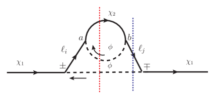
Figure 5: The two-loop self-energy diagram of $\chi_{1}$ contributing to the forbidden CP asymmetry. The outer vertices are fixed (from left to right) by $+-$ and $-+$ while the inner vertices $a,b$ are summed over thermal indices $\pm$. The arrows for the scalar propagators denote the momentum flow, and the fermion arrows align with the momentum flow. Qualitatively, the red cutting line induces scattering processes mediated by leptons, and the blue cutting line corresponds to scalar decay and inverse decay if $m_{\phi}>m_{\chi_{1}},m_{\chi_{2}}$.

In Eqs. (58)-(59), $i\not{S}^{<}_{\ell_{ij}}$ denotes the resummed lepton propagators. Summing over the thermal indices $\pm$ for $a,b$ in Fig. 5, we can write

$$i\not{{S}}^{<}_{\ell_{ij}} =(i\not{{S}}^{R}_{\ell_{i}})(-i\not{\Sigma}^{T}_{\ell_{ij}})(i\not{{S}}^{<}_{\ell_{j}})+(i\not{{S}}^{R}_{\ell_{i}})(-i\not{\Sigma}^{<}_{\ell_{ij}})(i\not{{S}}^{R}_{\ell_{j}})+(i\not{{S}}^{<}_{\ell_{i}})(-i\not{\Sigma}^{<}_{\ell_{ij}})(i\not{{S}}^{R}_{\ell_{j}})$$

$$-(i\not{{S}}^{R}_{\ell_{i}})(-i\not{\Sigma}^{<}_{\ell_{ij}})(i\not{{S}}^{>}_{\ell_{j}})-(i\not{{S}}^{<}_{\ell_{i}})(-i\not{\Sigma}^{\bar{T}}_{\ell_{ij}})(i\not{{S}}^{R}_{\ell_{j}})\,,$$ (62)

$$i\not{{S}}^{>}_{\ell_{ij}} =(i\not{{S}}^{>}_{\ell_{i}})(-i\not{\Sigma}^{T}_{\ell_{ij}})(i\not{{S}}^{R}_{\ell_{j}})+(i\not{{S}}^{R}_{\ell_{i}})(-i\not{\Sigma}^{>}_{\ell_{ij}})(i\not{{S}}^{R}_{\ell_{j}})+(i\not{{S}}^{R}_{\ell_{i}})(-i\not{\Sigma}^{>}_{\ell_{ij}})(i\not{{S}}^{<}_{\ell_{j}})$$

$$-(i\not{{S}}^{>}_{\ell_{i}})(-i\not{\Sigma}^{>}_{\ell_{ij}})(i\not{{S}}^{R}_{\ell_{j}})-(i\not{{S}}^{R}_{\ell_{i}})(-i\not{\Sigma}^{\bar{T}}_{\ell_{ij}})(i\not{{S}}^{>}_{\ell_{j}})\,,$$ (63)

where Eqs. (24) and (61) have been used and the minus sign from thermal index $a$ or $b$ being of the negative type has been included. In addition, we have applied Eqs. (36)-(37) such that $i{{S}}^{<}_{\ell_{i}}(p)\times i{{S}}^{>}_{\ell_{j}}(p)\propto\delta(p^{2}-2\tilde{m}_{i}^{2})\delta(p^{2}-2\tilde{m}_{j}^{2})=0$. Given $\not{{S}}^{>}_{\ell_{ij}}\propto y_{i2}^{\prime*}y^{\prime}_{j2}$, we play the trick of interchanging dummy indices $i,j$, so that Eq. (59) becomes

$$i\not{\Sigma}_{\chi_{1}}^{>}(p)=2(y^{\prime}_{i1}y^{\prime*}_{j1}y_{i2}^{\prime*}y^{\prime}_{j2})^{*}\int\frac{d^{4}p_{\ell}}{(2\pi)^{4}}\frac{d^{4}p_{\phi}}{(2\pi)^{4}}(2\pi)^{4}\delta^{4}(p-p_{\ell}+p_{\phi})P_{L}i\not{\tilde{S}}^{>}_{\ell_{ji}}P_{R}iG_{\phi}^{<}\,,$$ (64)

where the Yukawa couplings are factored out from $-i\not{\Sigma}_{\ell_{ij}}\equiv y^{\prime*}_{i2}y^{\prime}_{j2}\times(-i\not{\Sigma}_{\ell})$, with

$$i\not{{S}}^{>}_{\ell_{ji}} =(i\not{{S}}^{R}_{\ell_{i}})(-i\not{\Sigma}^{T}_{\ell})(i\not{{S}}^{>}_{\ell_{j}})+(i\not{{S}}^{R}_{\ell_{i}})(-i\not{\Sigma}^{>}_{\ell})(i\not{{S}}^{R}_{\ell_{j}})+(i\not{{S}}^{<}_{\ell_{i}})(-i\not{\Sigma}^{>}_{\ell})(i\not{{S}}^{R}_{\ell_{j}})$$

$$-(i\not{{S}}^{R}_{\ell_{i}})(-i\not{\Sigma}^{>}_{\ell})(i\not{{S}}^{>}_{\ell_{j}})-(i\not{{S}}^{>}_{\ell_{i}})(-i\not{\Sigma}^{\bar{T}}_{\ell})(i\not{{S}}^{R}_{\ell_{j}})\,.$$ (65)

Note that we have used the following relations:

$$(i\not{{S}}^{R}_{\ell_{i}})(-i\not{\Sigma}_{\ell})(i\not{{S}}^{<,>}_{\ell_{j}}) =(i\not{{S}}^{<,>}_{\ell_{j}})(-i\not{\Sigma}_{\ell})(i\not{{S}}^{R}_{\ell_{i}})\,,$$ (66)

$$(i\not{{S}}^{R}_{\ell_{i}})(-i\not{\Sigma}_{\ell})(i\not{{S}}^{R}_{\ell_{j}}) =(i\not{{S}}^{R}_{\ell_{j}})(-i\not{\Sigma}_{\ell})(i\not{{S}}^{R}_{\ell_{i}})\,,$$ (67)

since the resummed retarded propagator and Wightman functions depend on the same helicity operator $P_{\pm}$.

In the weak washout regime where the distribution functions of $\chi_{1},\bar{\chi}_{1}$ can be neglected, we can write down the CP-violating source $\mathcal{S}_{\rm CP}$ from Eq. (49) as

$$\mathcal{S}_{\rm CP}(p)=\frac{1}{2}\int\frac{d^{4}p}{(2\pi)^{4}}(2\pi)\delta(p^{2}-m_{\chi_{1}}^{2})\text{Tr}[\not{K}\not{p}]\,,$$ (68)

where $\not{K}$ is defined as $\not{K}(p)\equiv\theta(-p_{0})i\not{\Sigma}_{\chi_{1}}^{>}-\theta(p_{0})i\not{\Sigma}_{\chi_{1}}^{<}$ and is given by

$$\not{K}(p) =-2\int\frac{d^{4}p_{\ell}}{(2\pi)^{4}}\frac{d^{4}p_{\phi}}{(2\pi)^{4}}(2\pi)^{4}\delta^{4}(p-p_{\ell}+p_{\phi})\sum_{i=1}^{5}\mathcal{I}_{i}\,,$$ (69)

with the five $\mathcal{I}_{i}$ functions from the difference of Eq. (C) and (C):

$$\mathcal{I}_{1} =i\not{{S}}^{R}_{\ell_{i}}\left[Y_{4}^{*}\theta(-p_{0})e^{p_{\ell 0}/T}iG_{\phi}^{<}(-i\not{\Sigma}^{T}_{\ell})+Y_{4}\theta(p_{0})iG_{\phi}^{>}(-i\not{\Sigma}^{T}_{\ell})\right]i\not{{S}}^{<}_{\ell_{j}}\,,$$ (70)

$$\mathcal{I}_{2} =-i\not{{S}}^{R}_{\ell_{i}}\left[Y_{4}^{*}\theta(-p_{0})iG_{\phi}^{<}(-i\not{\Sigma}^{>}_{\ell})-Y_{4}\theta(p_{0})iG_{\phi}^{>}(-i\not{\Sigma}^{<}_{\ell})\right]i\not{{S}}^{R}_{\ell_{j}}\,,$$ (71)

$$\mathcal{I}_{3} =-i\not{{S}}^{<}_{\ell_{i}}\left[Y_{4}^{*}\theta(-p_{0})iG_{\phi}^{<}(-i\not{\Sigma}^{>}_{\ell})-Y_{4}\theta(p_{0})iG_{\phi}^{>}(-i\not{\Sigma}^{<}_{\ell})\right]i\not{{S}}^{R}_{\ell_{j}}\,,$$ (72)

$$\mathcal{I}_{4} =-i\not{{S}}^{R}_{\ell_{i}}\left[Y_{4}^{*}\theta(-p_{0})e^{p_{\ell 0}/T}iG_{\phi}^{<}(-i\not{\Sigma}^{>}_{\ell})-Y_{4}\theta(p_{0})e^{p_{\ell 0}/T}iG_{\phi}^{>}(-i\not{\Sigma}^{<}_{\ell})\right]i\not{{S}}^{<}_{\ell_{j}}\,,$$ (73)

$$\mathcal{I}_{5} =-i\not{{S}}^{<}_{\ell_{i}}\left[Y_{4}^{*}\theta(-p_{0})e^{p_{\ell 0}/T}iG_{\phi}^{<}(-i\not{\Sigma}^{\bar{T}}_{\ell})+Y_{4}\theta(p_{0})iG_{\phi}^{>}(-i\not{\Sigma}^{\bar{T}}_{\ell})\right]i\not{{S}}^{R}_{\ell_{j}}\,.$$ (74)

Note that in Eq. (68), $m_{\chi_{2}}$ will not contribute in the Dirac trace since there is no chirality flip in the inner loop of Fig. 5. Besides, $\text{Tr}[\not{K}m_{\chi_{1}}]=0$ since $\not{K}$ contains an odd number of Dirac $\gamma$-matrices. The factor of $e^{p_{\ell 0}/T}$ in $\mathcal{I}_{1},\mathcal{I}_{4},\mathcal{I}_{5}$ arises from the KMS relation $\not{{S}}^{>}_{\ell}(p)=-e^{p_{0}/T}\not{S}_{\ell}^{<}(p)$, and we have defined

$$Y_{4}\equiv y^{\prime}_{i1}y^{\prime*}_{j1}y_{i2}^{\prime*}y^{\prime}_{j2}\,.$$ (75)

$\mathcal{I}_{3}$ and $\mathcal{I}_{5}$ can be rewritten as a product of $i{S}^{R}_{\ell_{i}}\times i{S}^{<}_{\ell_{j}}$ similar to $\mathcal{I}_{1}$ and $\mathcal{I}_{4}$. To this end, we interchange the dummy indices $i,j$ and use $Y_{4}(i\leftrightharpoons j)=Y_{4}^{*}$ as well as Eq. (66), resulting in

$$\mathcal{I}_{3} =-i\not{{S}}^{R}_{\ell_{i}}\left[Y_{4}\theta(-p_{0})iG_{\phi}^{<}(-i\not{\Sigma}^{>}_{\ell})-Y_{4}^{*}\theta(p_{0})iG_{\phi}^{>}(-i\not{\Sigma}^{<}_{\ell})\right]i\not{{S}}^{<}_{\ell_{j}}\,,$$ (76)

$$\mathcal{I}_{5} =-i\not{{S}}^{R}_{\ell_{i}}\left[Y_{4}\theta(-p_{0})e^{p_{\ell 0}/T}iG_{\phi}^{<}(-i\not{\Sigma}^{\bar{T}}_{\ell})+Y_{4}^{*}\theta(p_{0})iG_{\phi}^{>}(-i\not{\Sigma}^{\bar{T}}_{\ell})\right]i\not{{S}}^{<}_{\ell_{j}}\,.$$ (77)

After this performance, Eq. (69) will only contain products of $i{S}^{R}_{\ell_{i}}\times i{S}^{<}_{\ell_{j}}$ and $i{S}^{R}_{\ell_{i}}\times i{S}^{R}_{\ell_{j}}$.

The term $i{S}^{R}_{\ell_{i}}\times i{S}^{<}_{\ell_{j}}$ corresponds to making the lepton propagator of flavor $j$ onshell, i.e., the decay and inverse decay channels induced from the blue cutting line in Fig. 5, while the term $i{S}^{R}_{\ell_{i}}\times i{S}^{R}_{\ell_{j}}$ represents the scattering processes mediated by onshell and offshell lepton propagators induced from the red cutting line. The onshell scattering contribution is crucial to ensure that no CP asymmetry can arise from full thermal equilibrium, and hence to guarantee CPT theorem and unitarity. This contribution also corresponds to the effect that should be carefully subtracted in the Boltzmann equation, known as the real-intermediate-state subtraction Kolb:1979qa ; Giudice:2003jh . In the following calculation, we will take into account the onshell scattering effect but neglect the offshell contribution. It should be mentioned, however, in the strong washout regime, the offshell scattering contribution could be important to erase the CP asymmetry generated at earlier epochs.

To proceed, let us rewrite the CP-violating source in a compact form:

$$\mathcal{S}_{\rm CP}(p)=-\int\frac{d^{4}p}{(2\pi)^{4}}\int\frac{d^{4}p_{\ell}}{(2\pi)^{4}}\int\frac{d^{4}p_{\phi}}{(2\pi)^{4}}(2\pi)^{5}\delta^{4}(p-p_{\ell}+p_{\phi})\delta(p^{2}-m_{\chi_{1}}^{2})\sum_{i=1}^{5}\mathcal{S}_{\text{CP}i}\,,$$ (78)

where $\mathcal{S}_{\text{CP}i}\equiv\text{Tr}[\mathcal{I}_{i}\not{p}]$. For the moment, we take the thermal distribution for leptons, but allow nonthermal distributions for scalar $\phi$ and fermion $\chi_{2}$. As will be shown below, the distributions of $\phi$ and $\chi_{2}$ in the inner loop of Fig. 5 determine if the forbidden CP asymmetry can arise. In particular, for $\phi$ and $\chi_{2}$ in full thermal equilibrium, there is no forbidden CP asymmetry of $\chi_{1}$. To parameterize the departure from thermal equilibrium, we define $f_{i}=f_{i}^{\rm eq}+\delta f_{i}$ for $i=\phi,\chi_{2}$, with the approximation $\delta f_{i}=\delta\bar{f}_{i}$. This treatment assumes that there are no large initial asymmetries of $\phi,\chi_{2}$. For example, both $\phi$ and $\chi_{2}$ are initially in thermal equilibrium ($T>m_{\phi}$) prior to the onset of the leptogenesis epoch ($T\lesssim m_{\phi}$). Accordingly, we can write the propagators and self-energy amplitudes as

$$iG^{ab}_{\phi}(p) =iG^{ab,\rm eq}_{\phi}(p)+i\delta G_{\phi}(p)\,,$$ (79)

$$i\not{S}^{ab}_{\chi_{2}}(p) =i\not{S}^{ab,\rm eq}_{\chi_{2}}(p)+i\delta\not{S}_{\chi_{2}}(p)\,,$$ (80)

$$i\not{\Sigma}_{\ell}^{ab}(p) =i\not{\Sigma}_{\ell}^{ab,\rm eq}(p)+i\delta\not{\Sigma}_{\ell}^{ab}(p)\,,$$ (81)

where $a,b=\pm$, and

$$i\delta G_{\phi}(p) =2\pi\delta(p^{2}-m_{\phi}^{2})\delta f_{\phi}(|p_{0}|)\,,$$ (82)

$$i\delta\not{S}_{\chi_{2}}(p) =-2\pi\delta(p^{2}-m_{\chi_{2}}^{2})(\not{p}+m_{\chi_{2}})\delta f_{\chi_{2}}(|p_{0}|)\,,$$ (83)

$$i\not{\Sigma}_{\ell}^{ab,\rm eq}(p_{\ell}) =\int\frac{d^{4}q}{(2\pi)^{4}}\frac{d^{4}q_{\phi}}{(2\pi)^{4}}(2\pi)^{4}\delta^{4}(q-q_{\phi}-p_{\ell})P_{R}i\not{S}_{\chi_{2}}^{ab,\rm eq}P_{L}iG_{\phi}^{ba,\rm eq}\,,$$ (84)

$$i\delta\not{\Sigma}_{\ell}^{ab}(p_{\ell}) =\int\frac{d^{4}q}{(2\pi)^{4}}\frac{d^{4}q_{\phi}}{(2\pi)^{4}}(2\pi)^{4}\delta^{4}(q-q_{\phi}-p_{\ell})\left(P_{R}i\not{S}_{\chi_{2}}^{ab,\rm eq}P_{L}i\delta G_{\phi}+P_{R}i\delta\not{S}_{\chi_{2}}P_{L}iG^{ba,\rm eq}_{\phi}\right)\,,$$ (85)

with $q,q_{\phi}$ the inner loop momenta of $\chi_{2}$ and $\phi$. Note that we have only kept the linear deviation of thermal distributions in $i\delta\not{\Sigma}_{\ell}^{ab}$.

There are two terms in each $\mathcal{S}_{\text{CP}i}$, corresponding to positive and negative frequencies of $\chi_{1}$. Note that the presence of $iG_{\phi}^{<,>}$ from the outer loop dictates the kinetic threshold via $\delta(p_{\phi}^{2}-m_{\phi}^{2})$. For $m_{\chi_{1}}^{2}+2\tilde{m}_{i}^{2}<m_{\phi}^{2}$ we obtain two kinetic regions:

$$\theta(-p_{0})\theta(p_{\ell 0})\,,\quad\theta(p_{0})\theta(-p_{\ell 0})\,.$$ (86)

Using these regions and the symmetries of the full momentum integration, we can simplify the $\theta(-p_{0})$ and $\theta(p_{0})$ terms in each $\mathcal{S}_{\text{CP}i}$. Starting with $\mathcal{S}_{\text{CP}1}$, we see that for the $\theta(-p_{0})$ term, only the positive lepton frequency from $i\not{S}_{\ell_{j}}^{<}$ is selected, and the resonance would appear in the $P_{-}$ component of $\not{S}^{R}_{\ell_{i}}$. Analogously, the negative lepton frequency from $i\not{S}_{\ell_{j}}^{<}$ is selected in the $\theta(p_{0})$ term and the resonance would appear in the $P_{+}$ component of $\not{S}^{R}_{\ell_{i}}$. Consequently, we obtain the $\theta(-p_{0})$ and $\theta(p_{0})$ terms of $\mathcal{S}_{\text{CP}1}$:

$$\mathcal{S}_{\text{CP}1}[\theta(-p_{0})] =\frac{-i\pi Y_{4}^{*}}{2(\tilde{m}_{j}^{2}-\tilde{m}_{i}^{2})}\theta(-p_{0})e^{p_{\ell 0}/T}iG_{\phi}^{<}(-i\Sigma^{T}_{\ell})\text{sign}(p_{\ell 0})f_{\ell}(p_{\ell 0})\frac{\delta(p_{\ell 0}-\omega_{j})}{\omega_{j}}\text{Tr}\left[P_{L}\not{p}_{\ell}P_{R}\not{q}P_{L}\not{p}_{\ell}P_{R}\not{p}\right],$$ (87)

$$\mathcal{S}_{\text{CP}1}[\theta(p_{0})] =\frac{-i\pi Y_{4}}{2(\tilde{m}_{j}^{2}-\tilde{m}_{i}^{2})}\theta(p_{0})iG_{\phi}^{>}(-i\Sigma^{T}_{\ell})\text{sign}(p_{\ell 0})f_{\ell}(p_{\ell 0})\frac{\delta(p_{\ell 0}+\omega_{j})}{\omega_{j}}\text{Tr}\left[P_{L}\not{p}_{\ell}P_{R}\not{q}P_{L}\not{p}_{\ell}P_{R}\not{p}\right],$$ (88)

where we have factored out the Dirac matrices from $-i\not{\Sigma}^{T}_{\ell}$ via $-i\not{\Sigma}^{T}_{\ell}=-i\Sigma^{T}_{\ell}\times(P_{R}\not{q}P_{L})$. By applying $p_{i}\to-p_{i}$ for all momenta to Eq. (87) and using

$$G_{\phi}^{<}(-p)=G_{\phi}^{>}(p)\,,\quad\Sigma^{T}_{\ell}(-p)=\Sigma^{T}_{\ell}(p)\,,\quad e^{-p_{\ell 0}/T}f_{\ell}(-p_{\ell 0})=f_{\ell}(p_{\ell 0})\,,$$ (89)

we obtain a simplified $\mathcal{S}_{\text{CP}1}$:

$$\mathcal{S}_{\text{CP}1} =\frac{\pi\text{Im}(Y_{4})}{\tilde{m}_{j}^{2}-\tilde{m}_{i}^{2}}\theta(p_{0})iG_{\phi}^{>}(-i\Sigma^{T}_{\ell})\text{sign}(p_{\ell 0})f_{\ell}(p_{\ell 0})\frac{\delta(p_{\ell 0}+\omega_{j})}{\omega_{j}}\text{Tr}\left[P_{L}\not{p}_{\ell}P_{R}\not{q}P_{L}\not{p}_{\ell}P_{R}\not{p}\right].$$ (90)

The above analysis can be directly applied to $\mathcal{S}_{\text{CP}5}$ with $\mathcal{I}_{5}$ given by Eq. (77). We obtain the same expression for $\mathcal{S}_{\text{CP}5}$ except for the $\Sigma_{\ell}$ dependence:

$$\mathcal{S}_{\text{CP}5} =\frac{\pi\text{Im}(Y_{4})}{\tilde{m}_{j}^{2}-\tilde{m}_{i}^{2}}\theta(p_{0})iG_{\phi}^{>}(-i\Sigma^{\bar{T}}_{\ell})\text{sign}(p_{\ell 0})f_{\ell}(p_{\ell 0})\frac{\delta(p_{\ell 0}+\omega_{j})}{\omega_{j}}\text{Tr}\left[P_{L}\not{p}_{\ell}P_{R}\not{q}P_{L}\not{p}_{\ell}P_{R}\not{p}\right].$$ (91)

Next, let us turn to $\mathcal{S}_{\text{CP}3}$ with $\mathcal{I}_{3}$ given by Eq. (76). We can analogously write the $\theta(-p_{0})$ and $\theta(p_{0})$ terms as

$$\mathcal{S}_{\text{CP}3}[\theta(-p_{0})] =\frac{i\pi Y_{4}}{2(\tilde{m}_{j}^{2}-\tilde{m}_{i}^{2})}\theta(-p_{0})iG_{\phi}^{<}(-i\Sigma_{\ell}^{>})\text{sign}(p_{\ell 0})f_{\ell}(p_{\ell 0})\frac{\delta(p_{\ell 0}-\omega_{j})}{\omega_{j}}\text{Tr}\left[P_{L}\not{p}_{\ell}P_{R}\not{q}P_{L}\not{p}_{\ell}P_{R}\not{p}\right],$$ (92)

$$\mathcal{S}_{\text{CP}3}[\theta(p_{0})] =\frac{-i\pi Y_{4}^{*}}{2(\tilde{m}_{j}^{2}-\tilde{m}_{i}^{2})}\theta(p_{0})iG_{\phi}^{>}(-i\Sigma_{\ell}^{<})\text{sign}(p_{\ell 0})f_{\ell}(p_{\ell 0})\frac{\delta(p_{\ell 0}+\omega_{j})}{\omega_{j}}\text{Tr}\left[P_{L}\not{p}_{\ell}P_{R}\not{q}P_{L}\not{p}_{\ell}P_{R}\not{p}\right].$$ (93)

By applying $p_{i}\to-p_{i}$ to Eq. (92) and using Eq. (89) as well as

$$i\Sigma_{\ell}^{>}(-p)=i\Sigma_{\ell}^{<}(p)\,,\quad f_{\ell}(-p_{\ell 0})+f_{\ell}(p_{\ell 0})=1\,,$$ (94)

we arrive at

$$\mathcal{S}_{\text{CP}3} =\frac{-i\pi Y_{4}}{2(\tilde{m}_{j}^{2}-\tilde{m}_{i}^{2})}\theta(p_{0})iG_{\phi}^{>}(-i\Sigma_{\ell}^{<})\text{sign}(p_{\ell 0})\frac{\delta(p_{\ell 0}+\omega_{j})}{\omega_{j}}\text{Tr}\left[P_{L}\not{p}_{\ell}P_{R}\not{q}P_{L}\not{p}_{\ell}P_{R}\not{p}\right]$$

$$-\frac{\pi\text{Im}(Y_{4})}{\tilde{m}_{j}^{2}-\tilde{m}_{i}^{2}}\theta(p_{0})iG_{\phi}^{>}(-i\Sigma_{\ell}^{<})\text{sign}(p_{\ell 0})f_{\ell}(p_{\ell 0})\frac{\delta(p_{\ell 0}+\omega_{j})}{\omega_{j}}\text{Tr}\left[P_{L}\not{p}_{\ell}P_{R}\not{q}P_{L}\not{p}_{\ell}P_{R}\not{p}\right].$$ (95)

Using the same trick, we find that

$$\mathcal{S}_{\text{CP}4}=\mathcal{S}_{\text{CP}3}\,.$$ (96)

The simplified $\mathcal{S}_{\text{CP}1},\mathcal{S}_{\text{CP}3},\mathcal{S}_{\text{CP}4},\mathcal{S}_{\text{CP}5}$ all have the same correspondence to the decay and inverse decay processes, which are induced by the blue cutting line shown in Fig. 5. The remaining $\mathcal{S}_{\text{CP}2}$ has a different structure, which is characterized by the product of two retarded propagators. This term has two scattering channels mediated by resummed leptons of flavor $i$ and $j$, which corresponds to onshell $\not{S}^{R}_{\ell_{i}}$ and onshell $\not{S}^{R}_{\ell_{j}}$ respectively. Using Eq. (35) for flavor $i$ and $j$ separately and then interchanging the dummy indices $i,j$ for onshell flavor $i$, we arrive at

$$\mathcal{S}_{\text{CP}2}=\frac{i\pi(Y_{4}^{*}+Y_{4})}{2(\tilde{m}_{j}^{2}-\tilde{m}_{i}^{2})}\theta(p_{0})iG_{\phi}^{>}(-i\Sigma_{\ell}^{<})\text{sign}(p_{\ell 0})\frac{\delta(p_{\ell 0}+\omega_{j})}{\omega_{j}}\text{Tr}\left[P_{L}\not{p}_{\ell}P_{R}\not{q}P_{L}\not{p}_{\ell}P_{R}\not{p}\right].$$ (97)

We see that the $Y_{4}$ dependence of $\mathcal{S}_{\text{CP}2}$ is to be combined with that of $\mathcal{S}_{\text{CP}3},\mathcal{S}_{\text{CP}4}$, leading to a CP-violating source that depends only on the imaginary part of Yukawa couplings: $\text{Im}(Y_{4})$.

Assembling the five $\mathcal{S}_{\text{CP}i}$, we arrive at

$$\mathcal{S}_{\rm CP}(p) =\frac{\pi\text{Im}(Y_{4})}{\tilde{m}_{j}^{2}-\tilde{m}_{i}^{2}}\int\frac{d^{4}p}{(2\pi)^{4}}\int\frac{d^{4}p_{\ell}}{(2\pi)^{4}}\int\frac{d^{4}p_{\phi}}{(2\pi)^{4}}(2\pi)^{5}\delta^{4}(p-p_{\ell}+p_{\phi})\delta(p^{2}-m_{\chi_{1}}^{2})\theta(p_{0})\text{sign}(p_{\ell 0})$$

$$\times iG_{\phi}^{>}\left\{\left(i\Sigma_{\ell}^{>}-i\Sigma_{\ell}^{<}\right)f_{\ell}(p_{\ell 0})+i\Sigma_{\ell}^{<}\right\}\frac{\delta(p_{\ell 0}+\omega_{j})}{\omega_{j}}\text{Tr}\left[P_{L}\not{p}_{\ell}P_{R}\not{q}P_{L}\not{p}_{\ell}P_{R}\not{p}\right].$$ (98)

We see that for thermal $\phi$ and $\chi_{2}$, the KMS relation holds $\Sigma_{\ell}^{>}(p)=-e^{p_{0}/T}\Sigma_{\ell}^{<}(p)$. Consequently, the terms in the curly bracket sum to zero:

$$\left[i\Sigma_{\ell}^{>,\rm eq}(p_{\ell})-i\Sigma_{\ell}^{<,\rm eq}(p_{\ell})\right]f_{\ell}(p_{\ell 0})+i\Sigma_{\ell}^{<,\rm eq}(p_{\ell})=0\,.$$ (99)

Therefore, a nonthermal $\chi_{1}$ is not sufficient to generate a nonzero forbidden CP asymmetry and at least $\phi$ or $\chi_{2}$ should additionally be out of equilibrium during the leptogenesis epoch.

For $m_{\phi}\gg m_{\chi_{2}}$, the scalar starts to significantly depart from thermal equilibrium at $T<m_{\phi}$. In this epoch, $\chi_{2}$ is still relativistic, such that scattering between $\chi_{2}$ and the SM plasma is strong enough to keep $\chi_{2}$ in thermal equilibrium, provided the Yukawa coupling is not too small. Therefore, we will take the thermal distribution for $\chi_{2}$ to evaluate Eq. (C). Substituting Eqs. (79) and (81) into Eq. (C) and using Eq. (99), we obtain the $iG_{\phi}^{>}\times\{...\}$ term of Eq. (C) at linear order of nonthermal distribution functions:

$$iG_{\phi}^{>,\rm eq}\left\{(i\delta\Sigma_{\ell}^{>}-i\delta\Sigma_{\ell}^{<})f_{\ell}(p_{\ell 0})+i\delta\Sigma_{\ell}^{<}\right\},$$ (100)

where the curly bracket term reads

$$\{...\}=\int\frac{d^{4}q_{\phi}}{(2\pi)^{4}}d^{4}q\delta^{4}(q-q_{\phi}-p_{\ell})\delta(q^{2}-m_{\chi_{2}}^{2})\delta(q_{\phi}^{2}-m_{\phi}^{2})\delta f_{\phi}(|q_{\phi 0}|)\left[\text{sign}(q_{0})f_{\ell}(p_{\ell 0})-f_{\chi_{2}}(|q_{0}|)+\theta(-q_{0})\right].$$ (101)

The Dirac $\delta$-functions dictate the kinetic regions. From $\delta(q^{2}-m_{\chi_{2}}^{2})$ and $\delta(q_{\phi}^{2}-m_{\phi}^{2})$, together with the second kinetic region given in Eq. (86), we obtain

$$q_{\phi 0}>0,\quad q_{0}>0\,,$$ (102)

and Eq. (101) reduces to

$$\{...\}=\frac{1}{4(2\pi)^{3}p_{\ell}}\int^{\infty}_{\frac{m_{\phi}^{2}}{4p_{\ell}}+p_{\ell}}dE^{\prime}_{\phi}\delta_{\phi}(E^{\prime}_{\phi})\left[1-f_{\chi_{2}}(E^{\prime}_{\phi}-p_{\ell})-f_{\ell}(p_{\ell})\right],$$ (103)

where $E^{\prime}_{\phi}=|q_{\phi 0}|$, the lower integration limit comes from the angular integration with $\delta(m_{\phi}^{2}-2E^{\prime}_{\phi}p_{\ell}+2p_{\ell}q_{\phi}\cos\theta)$, and we have used $f_{\ell}(p_{\ell 0})=1-f_{\ell}(-p_{\ell 0})$ for $p_{\ell 0}=-\omega_{j}$ with the approximation $\omega_{j}\approx|\vec{p}_{\ell}|\equiv p_{\ell}$.

Integrating over $d^{4}p$ via $\delta^{4}(p-p_{\ell}+p_{\phi})$ in Eq. (C), $dp_{\ell 0}$ via $\delta(p_{\ell 0}+\omega_{j})$, and $dp_{\phi 0}$ via $\delta(p_{\phi 0}+E_{\phi})$ (from $iG_{\phi}^{>,\rm eq}$), we finally arrive at the result presented in the main text:

$$S_{\rm CP}=-\frac{\text{Im}(Y_{4})m_{\phi}^{4}}{256\pi^{4}(\tilde{m}_{j}^{2}-\tilde{m}_{i}^{2})}\int^{\infty}_{0}\frac{dp_{\ell}}{p_{\ell}}\int^{\infty}_{\frac{m_{\phi}^{2}}{4p_{\ell}}+p_{\ell}}dE_{\phi}\int^{\infty}_{\frac{m_{\phi}^{2}}{4p_{\ell}}+p_{\ell}}dE^{\prime}_{\phi}f_{\phi}(E_{\phi})\delta f_{\phi}(E^{\prime}_{\phi})\left[1-f_{\chi_{2}}(E^{\prime}_{\phi}-p_{\ell})-f_{\ell}(p_{\ell})\right],$$ (104)

where $E_{\phi}=|p_{\phi 0}|$, $\text{Tr}[P_{L}\not{p}_{\ell}P_{R}\not{q}P_{L}\not{p}_{\ell}P_{R}\not{p}]=4(p\cdot p_{\ell})(q\cdot p_{\ell})-2p_{\ell}^{2}(p\cdot q)\approx m_{\phi}^{4}$ was used in the limit $m_{\phi}^{2}\gg\tilde{m}_{j}^{2},m_{\chi_{1}}^{2},m_{\chi_{2}}^{2}$, and the lower integration limit of $E_{\phi}$ comes from the angular integration with $\delta(m_{\phi}^{2}-2E_{\phi}p_{\ell}+2p_{\ell}p_{\phi}\cos\theta)$. It is worth mentioning that the scaling $1/p_{\ell}$ in the $p_{\ell}$ integration will not lead to IR divergence. This can be seen by taking $p_{\ell}\to 0$ in the lower $E_{\phi},E^{\prime}_{\phi}$ integration limits, which makes the integration turn to zero.

References

(1)Planck Collaboration, N. Aghanim et al., Planck 2018 results. VI.
Cosmological parameters, Astron. Astrophys.641 (2020) A6,
[arXiv:1807.06209]. [Erratum:
Astron.Astrophys. 652, C4 (2021)].
(2)
M. Fukugita and T. Yanagida, Baryogenesis Without Grand Unification,
Phys. Lett. B174 (1986) 45–47.
(3)
M. A. Luty, Baryogenesis via leptogenesis, Phys. Rev. D45
(1992) 455–465.
(4)
L. Covi, E. Roulet, and F. Vissani, CP violating decays in leptogenesis
scenarios, Phys. Lett. B384 (1996) 169–174,
[hep-ph/9605319].
(5)
G. F. Giudice, A. Notari, M. Raidal, A. Riotto, and A. Strumia, Towards a
complete theory of thermal leptogenesis in the SM and MSSM, Nucl.
Phys. B685 (2004) 89–149,
[hep-ph/0310123].
(6)
W. Buchmuller, P. Di Bari, and M. Plumacher, Leptogenesis for
pedestrians, Annals Phys.315 (2005) 305–351,
[hep-ph/0401240].
(7)
S. Davidson, E. Nardi, and Y. Nir, Leptogenesis, Phys. Rept.466 (2008) 105–177, [arXiv:0802.2962].
(8)
C. S. Fong, E. Nardi, and A. Riotto, Leptogenesis in the Universe,
Adv. High Energy Phys.2012 (2012) 158303,
[arXiv:1301.3062].
(9)
L. Covi and E. Roulet, Baryogenesis from mixed particle decays, Phys. Lett. B399 (1997) 113–118,
[hep-ph/9611425].
(10)
E. Ma and U. Sarkar, Neutrino masses and leptogenesis with heavy Higgs
triplets, Phys. Rev. Lett.80 (1998) 5716–5719,
[hep-ph/9802445].
(11)
K. Dick, M. Lindner, M. Ratz, and D. Wright, Leptogenesis with Dirac
neutrinos, Phys. Rev. Lett.84 (2000) 4039–4042,
[hep-ph/9907562].
(12)
H. Murayama and A. Pierce, Realistic Dirac leptogenesis, Phys.
Rev. Lett.89 (2002) 271601,
[hep-ph/0206177].
(13)
V. A. Kuzmin, V. A. Rubakov, and M. E. Shaposhnikov, On the Anomalous
Electroweak Baryon Number Nonconservation in the Early Universe, Phys. Lett. B155 (1985) 36.
(14)
H. A. Weldon, Simple Rules for Discontinuities in Finite Temperature
Field Theory, Phys. Rev. D28 (1983) 2007.
(15)
K.-c. Chou, Z.-b. Su, B.-l. Hao, and L. Yu, Equilibrium and
Nonequilibrium Formalisms Made Unified, Phys. Rept.118 (1985)
1–131.
(16)
E. Calzetta and B. L. Hu, Nonequilibrium Quantum Fields: Closed Time Path
Effective Action, Wigner Function and Boltzmann Equation, Phys. Rev.
D37 (1988) 2878.
(17)
J. Berges, Introduction to nonequilibrium quantum field theory, AIP Conf. Proc.739 (2004), no. 1 3–62,
[hep-ph/0409233].
(18)
M. Garny, A. Hohenegger, A. Kartavtsev, and M. Lindner, Systematic
approach to leptogenesis in nonequilibrium QFT: Self-energy contribution to
the CP-violating parameter, Phys. Rev. D81 (2010) 085027,
[arXiv:0911.4122].
(19)
M. Beneke, B. Garbrecht, M. Herranen, and P. Schwaller, Finite Number
Density Corrections to Leptogenesis, Nucl. Phys. B838 (2010)
1–27, [arXiv:1002.1326].
(20)
B. Garbrecht, Leptogenesis: The Other Cuts, Nucl. Phys. B847 (2011) 350–366, [arXiv:1011.3122].
(21)
M. Garny, A. Hohenegger, and A. Kartavtsev, Medium corrections to the
CP-violating parameter in leptogenesis, Phys. Rev. D81 (2010)
085028, [arXiv:1002.0331].
(22)
M. Beneke, B. Garbrecht, C. Fidler, M. Herranen, and P. Schwaller, Flavoured Leptogenesis in the CTP Formalism, Nucl. Phys. B843 (2011) 177–212, [arXiv:1007.4783].
(23)
M. Drewes and B. Garbrecht, Leptogenesis from a GeV Seesaw without Mass
Degeneracy, JHEP03 (2013) 096,
[arXiv:1206.5537].
(24)
B. Garbrecht and M. Herranen, Effective Theory of Resonant Leptogenesis
in the Closed-Time-Path Approach, Nucl. Phys. B861 (2012)
17–52, [arXiv:1112.5954].
(25)
M. Garny, A. Kartavtsev, and A. Hohenegger, Leptogenesis from first
principles in the resonant regime, Annals Phys.328 (2013)
26–63, [arXiv:1112.6428].
(26)
P. S. Bhupal Dev, P. Millington, A. Pilaftsis, and D. Teresi, Kadanoff–Baym approach to flavour mixing and oscillations in
resonant leptogenesis, Nucl. Phys. B891 (2015) 128–158,
[arXiv:1410.6434].
(27)
T. Frossard, M. Garny, A. Hohenegger, A. Kartavtsev, and D. Mitrouskas, Systematic approach to thermal leptogenesis, Phys. Rev. D87
(2013), no. 8 085009, [arXiv:1211.2140].
(28)
B. Garbrecht, Leptogenesis from Additional Higgs Doublets, Phys.
Rev. D85 (2012) 123509, [arXiv:1201.5126].
(29)
T. Hambye and D. Teresi, Higgs doublet decay as the origin of the baryon
asymmetry, Phys. Rev. Lett.117 (2016), no. 9 091801,
[arXiv:1606.00017].
(30)
T. Prokopec, M. G. Schmidt, and S. Weinstock, Transport equations for
chiral fermions to order h bar and electroweak baryogenesis. Part 1, Annals Phys.314 (2004) 208–265,
[hep-ph/0312110].
(31)
T. Prokopec, M. G. Schmidt, and S. Weinstock, Transport equations for
chiral fermions to order h-bar and electroweak baryogenesis. Part II, Annals Phys.314 (2004) 267–320,
[hep-ph/0406140].
(32)
B. Garbrecht, Baryogenesis from Mixing of Lepton Doublets, Nucl.
Phys. B868 (2013) 557–576,
[arXiv:1210.0553].
(33)
E. Braaten and R. D. Pisarski, Soft Amplitudes in Hot Gauge Theories: A
General Analysis, Nucl. Phys. B337 (1990) 569–634.
(34)
M. E. Carrington, D.-f. Hou, and M. H. Thoma, Equilibrium and
nonequilibrium hard thermal loop resummation in the real time formalism,
Eur. Phys. J. C7 (1999) 347–354,
[hep-ph/9708363].
(35)
M. Bellac, Thermal Field Theory.
Cambridge University Press, 2000.
(36)
H. A. Weldon, Effective Fermion Masses of Order gT in High Temperature
Gauge Theories with Exact Chiral Invariance, Phys. Rev. D26
(1982) 2789.
(37)
A. Pilaftsis and T. E. J. Underwood, Resonant leptogenesis, Nucl.
Phys. B692 (2004) 303–345,
[hep-ph/0309342].
(38)
A. Pilaftsis and T. E. J. Underwood, Electroweak-scale resonant
leptogenesis, Phys. Rev. D72 (2005) 113001,
[hep-ph/0506107].
(39)
E. W. Kolb and S. Wolfram, Baryon Number Generation in the Early
Universe, Nucl. Phys. B172 (1980) 224. [Erratum: Nucl.Phys.B
195, 542 (1982)].
(40)
R. Kobes, Retarded functions, dispersion relations, and Cutkosky rules at
zero and finite temperature, Phys. Rev. D43 (1991)
1269–1282.
(43)
R. L. Kobes and G. W. Semenoff, Discontinuities of Green Functions in
Field Theory at Finite Temperature and Density, Nucl. Phys. B260 (1985) 714–746.
(44)
R. L. Kobes and G. W. Semenoff, Discontinuities of Green Functions in
Field Theory at Finite Temperature and Density. 2, Nucl. Phys. B272 (1986) 329–364.
(45)
E. K. Akhmedov, V. A. Rubakov, and A. Y. Smirnov, Baryogenesis via
neutrino oscillations, Phys. Rev. Lett.81 (1998) 1359–1362,
[hep-ph/9803255].
(46)
H. Davoudiasl, D. E. Morrissey, K. Sigurdson, and S. Tulin, Hylogenesis:
A Unified Origin for Baryonic Visible Matter and Antibaryonic Dark Matter,
Phys. Rev. Lett.105 (2010) 211304,
[arXiv:1008.2399].
(47)
C. Cheung and K. M. Zurek, Affleck-Dine Cogenesis, Phys. Rev. D84 (2011) 035007, [arXiv:1105.4612].
(48)
G. Elor, M. Escudero, and A. Nelson, Baryogenesis and Dark Matter from
Mesons, Phys. Rev. D99 (2019), no. 3 035031,
[arXiv:1810.00880].
(49)
J. A. Harvey and M. S. Turner, Cosmological baryon and lepton number in
the presence of electroweak fermion number violation, Phys. Rev. D42 (1990) 3344–3349.
(50)
See more details in the Supplemental Material.
(51)
C. P. Kiessig, M. Plumacher, and M. H. Thoma, Decay of a Yukawa fermion
at finite temperature and applications to leptogenesis, Phys. Rev. D82 (2010) 036007, [arXiv:1003.3016].
(52)
S.-P. Li, Dark matter freeze-in via a light fermion mediator: forbidden
decay and scattering, JCAP05 (2023) 008,
[arXiv:2301.02835].
(53)
M. D’Onofrio, K. Rummukainen, and A. Tranberg, Sphaleron Rate in the
Minimal Standard Model, Phys. Rev. Lett.113 (2014), no. 14
141602, [arXiv:1404.3565].
(54)
E. W. Kolb, The Early Universe, vol. 69.
Taylor and Francis, 5, 2019.
(55)
D. Wyler and L. Wolfenstein, Massless Neutrinos in Left-Right Symmetric
Models, Nucl. Phys. B218 (1983) 205–214.
(56)
R. N. Mohapatra and J. W. F. Valle, Neutrino Mass and Baryon Number
Nonconservation in Superstring Models, Phys. Rev. D34 (1986)
1642.
(57)
G. C. Branco, W. Grimus, and L. Lavoura, The Seesaw Mechanism in the
Presence of a Conserved Lepton Number, Nucl. Phys. B312
(1989) 492–508.
(58)
M. Shaposhnikov, A Possible symmetry of the nuMSM, Nucl. Phys. B763 (2007) 49–59, [hep-ph/0605047].
(59)
J. Kersten and A. Y. Smirnov, Right-Handed Neutrinos at CERN LHC and the
Mechanism of Neutrino Mass Generation, Phys. Rev. D76 (2007)
073005, [arXiv:0705.3221].
(60)
A. Abada, G. Arcadi, V. Domcke, and M. Lucente, Neutrino masses,
leptogenesis and dark matter from small lepton number violation?, JCAP12 (2017) 024, [arXiv:1709.00415].
(61)
A. Abada, G. Arcadi, V. Domcke, M. Drewes, J. Klaric, and M. Lucente, Low-scale leptogenesis with three heavy neutrinos, JHEP01
(2019) 164, [arXiv:1810.12463].
(62)
E. Braaten, R. D. Pisarski, and T.-C. Yuan, Production of Soft Dileptons
in the Quark - Gluon Plasma, Phys. Rev. Lett.64 (1990) 2242.
(63)
M. Drewes and J. U. Kang, The Kinematics of Cosmic Reheating, Nucl. Phys. B875 (2013) 315–350,
[arXiv:1305.0267]. [Erratum:
Nucl.Phys.B 888, 284–286 (2014)].