3-loop Feynman Integral Extrapolations for the Baseball Diagram

Abstract

We focus on numerical techniques for expanding 3-loop Feynman integrals with respect to the dimensional regularization parameter $\varepsilon,$ which is related to the space-time dimension as $\nu=4-2\varepsilon,$ and describes underlying UV singularities located at the boundaries of the integration domain. As a function of the squared momentum $s,$ the expansion coefficients exhibit thresholds that generally delineate regions for their computational techniques. For the problem at hand, a sequence of integrations with a linear extrapolation as $\varepsilon\rightarrow 0$ may be performed to determine leading coefficients of the $\varepsilon$-expansion numerically. For the “baseball” Feynman diagram, we have used extrapolation with respect to an additional parameter to improve the accuracy of the $\varepsilon$-expansion coefficients in case of singularities internal to the domain.

1 Introduction and Background

Higher order corrections are required for accurate theoretical prediction improvements in the technology of high energy physics experiments. Feynman loop integrals arise in the calculations of the Feynman diagrammatic approach, which is commonly used to address higher order corrections. Loop integrals may suffer from integrand singularities or irregularities at the boundaries and/or in the interior of the integration domain.

We recently explored methods for higher-order corrections to 2-loop Feynman integrals in the Euclidean or physical kinematical region [1], using numerical extrapolation and adaptive iterated integration. Our current goal is to address a 3-loop two-point integral for the “baseball” diagram of Figure 1 with six internal lines.

A representation of an $L$-loop Feynman integral with $N$ internal lines is given by (e.g., [2, 3, 4, 5])

$${\mathcal{F}}={\Gamma(N-\frac{\nu L}{2})}\,(-1)^{N}\int_{{\mathcal{C}}_{N}}\prod_{r=1}^{N}dx_{r}\,\delta(1-\sum x_{r})\,U^{-\nu/2}(V-i\varrho)^{\nu L/2-N}$$ (1)

$$\leavevmode\nobreak\ \leavevmode\nobreak\ \leavevmode\nobreak\ \leavevmode\nobreak\ \leavevmode\nobreak\ \mbox{or,\leavevmode\nobreak\ for\leavevmode\nobreak\ }L=3,N=6:$$

$${\mathcal{F}}={\Gamma(3\varepsilon)}\,\int_{{\mathcal{C}}_{6}}\prod_{r=1}^{6}dx_{r}\,\delta(1-\sum x_{r})\,U^{\leavevmode\nobreak\ \varepsilon-2}(V-i\varrho)^{-3\varepsilon}$$ (2)

where $V=M^{2}-W/U,\leavevmode\nobreak\ \leavevmode\nobreak\ M^{2}=\sum_{r}m_{r}^{2}x_{r}$;   $U$ and $W$ are polynomials determined by the topology of the corresponding diagram and physical parameters;  $\nu=4-2\varepsilon$ is the space-time dimension; $\varrho$ is a regularization parameter and we can set $\varrho=0$ unless $V$ vanishes in the domain;  ${\mathcal{C}}_{N}$ is the $N$-dimensional unit hypercube. We consider the integral without the prefactor $\Gamma(3\varepsilon).$

We use automatic integration, which is a black-box approach for producing (as outputs) an approximation $Qf$ to an integral $\mathcal{I}=\int_{\mathcal{D}}f(\vec{x})\leavevmode\nobreak\ d\vec{x}$ and an estimate ${\mathcal{E}}f$ of the actual error $Ef=|Qf-\mathcal{I}|,$ with the goal of satisfying an accuracy requirement of the form $|\,Qf-\mathcal{I}\,|\leavevmode\nobreak\ \leq\leavevmode\nobreak\ {\mathcal{E}}f\leavevmode\nobreak\ \leq\leavevmode\nobreak\ \max\,\{\,t_{a}\,,\,t_{r}\,|\mathcal{I}|\,\},$ where the integrand function $f,$ $d$-dimensional region $\mathcal{D}$ and (absolute/relative) error tolerances $t_{a}$ and $t_{r},$ respectively, are specified as part of the input.

For ultra-violet (UV) singularities at the boundaries of the domain, we make use of lattice rules for Quasi-Monte Carlo (QMC) integration [6] with a boundary transformation that is capable of smoothing singularities [7, 8]. Another non-adaptive approach is based on a double-exponential (DE) formula [9, 10, 11, 12]. Adaptive integration may be useful in fairly low dimensions to treat interior singularities by intensive region partitioning around hot spots [13, 14, 15]. We give results obtained with 1D iterated adaptive integration by the program Dqagse from the Quadpack package [13, 16]. In [1] we applied adaptive integration with an extrapolation on the parameter $\varrho$ that adjusts the factor in $V$ in the integrand denominator of Eq. (1). We termed the combined extrapolations in $\varepsilon$ and $\varrho$ as a “double extrapolation.”

Subsequently, Section 2 defines the baseball integral; linear extrapolation and double extrapolation methods are covered in Section 3; results are given in Section 4 and conclusions in Section 5.

2 Baseball integral

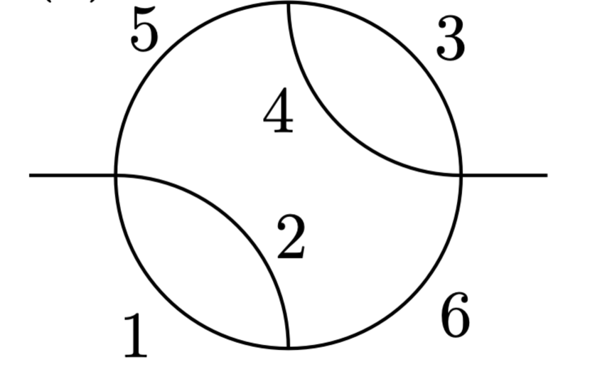
Figure 1: 3-loop baseball diagram with $N=6$ lines

A set of 3-loop diagrams with six internal lines, and their associated integrals are calculated by the authors after separating the ultra-violet divergence  [17]. It is our goal to demonstrate our techniques for numerical integration and extrapolation using another 3-loop diagram in the massive case. Hereafter, we assume that all masses of the internal lines equal 1. The derivation is based on a sector decomposition in 5D parameter space; thus the integrals are labeled by permutations of the 5-tuple $(1,2,3,4,5).$ There are $5!=120$ integrals, whereas many of the integrals may coincide through symmetries and the number of integrals to be computed is reduced. We deal with the baseball diagram shown in Figure 1. Then after assuming equal masses, 15 integrals remain. In this paper, we will study the ${\mathcal{I}}_{51234}$ integral of the baseball diagram, which is the integral that has the most singular UV divergence among the 15, with an ${\mathcal{O}}(\frac{1}{\varepsilon^{2}})$ term, and the rest start at the ${\mathcal{O}}(\frac{1}{\varepsilon})$ or ${\mathcal{O}}(1)$ order.

The integral is given by

$${\mathcal{I}_{51234}} = \int d\Gamma_{X}\leavevmode\nobreak\ t^{-1+2\varepsilon}v^{-1+\varepsilon}u^{\varepsilon}\,G^{-3\varepsilon}f^{-2+\varepsilon}=I_{00}+I_{01}+I_{10}+I_{11}$$ (3)

$$I_{00} = \frac{1}{\varepsilon^{2}}\frac{1}{2}\int d\Gamma_{0}\leavevmode\nobreak\ u^{\varepsilon}G_{0}^{-3\varepsilon}f_{0}^{-2+\varepsilon}$$ (4)

$$I_{01} = \frac{1}{\varepsilon}\frac{1}{2}\int d\Gamma_{a}\leavevmode\nobreak\ v^{-1+\varepsilon}u^{\varepsilon}\left(G_{a}^{-3\varepsilon}f_{a}^{-2+\varepsilon}-G_{0}^{-3\varepsilon}f_{0}^{-2+\varepsilon}\right)$$ (5)

$$I_{10} = \frac{1}{\varepsilon}\int d\Gamma_{b}\leavevmode\nobreak\ t^{-1+2\varepsilon}u^{\varepsilon}\left(G_{b}^{-3\varepsilon}f_{b}^{-2+\varepsilon}-G_{0}^{-3\varepsilon}f_{0}^{-2+\varepsilon}\right)$$ (6)

$$I_{11} = \int d\Gamma_{X}\leavevmode\nobreak\ t^{-1+2\varepsilon}v^{-1+\varepsilon}u^{\varepsilon}\times$$ (7)

$$\left(G^{-3\varepsilon}f^{-2+\varepsilon}-G_{a}^{-3\varepsilon}f_{a}^{-2+\varepsilon}-G_{b}^{-3\varepsilon}f_{b}^{-2+\varepsilon}+G_{0}^{-3\varepsilon}f_{0}^{-2+\varepsilon}\right)$$

$$= \int d\Gamma_{X}\leavevmode\nobreak\ t^{-1+2\varepsilon}v^{-1+\varepsilon}u^{\varepsilon}\left(G^{-3\varepsilon}f^{-2+\varepsilon}-G_{b}^{-3\varepsilon}f_{b}^{-2+\varepsilon}\right)$$

where

$$f = 1+w+u+uw+tu+tuw+tuvw+tu^{2}vw$$ (8)

$$f_{0} = f|_{t=0,v=0},\leavevmode\nobreak\ \leavevmode\nobreak\ f_{a}=f|_{t=0},\leavevmode\nobreak\ \leavevmode\nobreak\ f_{b}=f|_{v=0}$$ (9)

$$q = z(1-z)+wz(1-z)+uz(1-z)+uwz(1-z)+tuz+tuwz+tuvw(1-z)$$

$$+tu^{2}vw(1-z)+t^{2}u^{2}vw$$

$$q_{0} = q|_{t=0,v=0},\leavevmode\nobreak\ \leavevmode\nobreak\ q_{a}=q|_{t=0},\leavevmode\nobreak\ \leavevmode\nobreak\ q_{b}=q|_{v=0}$$ (10)

$$G = (1+t(1+u(1+v(1+w))))-s\frac{q}{f}$$ (11)

$$G_{0} = G|_{t=0,v=0},\leavevmode\nobreak\ \leavevmode\nobreak\ G_{a}=G|_{t=0},\leavevmode\nobreak\ \leavevmode\nobreak\ G_{b}=G|_{v=0}$$ (12)

and

$$\int d\Gamma_{X}=\int_{0}^{1}dz\int_{0}^{1}dt\int_{0}^{1}du\int_{0}^{1}dv\int_{0}^{1}dw,\leavevmode\nobreak\ \leavevmode\nobreak\ \leavevmode\nobreak\ \leavevmode\nobreak\ \leavevmode\nobreak\ \leavevmode\nobreak\ \int d\Gamma_{0}=\int_{0}^{1}dz\int_{0}^{1}du\int_{0}^{1}dw$$

$$\int d\Gamma_{a}=\int_{0}^{1}dz\int_{0}^{1}du\int_{0}^{1}dv\int_{0}^{1}dw,\leavevmode\nobreak\ \leavevmode\nobreak\ \leavevmode\nobreak\ \leavevmode\nobreak\ \leavevmode\nobreak\ \leavevmode\nobreak\ \leavevmode\nobreak\ \int d\Gamma_{b}=\int_{0}^{1}dz\int_{0}^{1}dt\int_{0}^{1}du\int_{0}^{1}dw$$

Note that $f_{0}=f_{a},$ $q_{0}=q_{a}$ and $G_{0}=G_{a};$ thus the integrand of Eq. (5) is zero, and $I_{11}$ simplifies to Eq. (7). Here, $s$ equals $s=P^{2}$, where $P$ is the external momentum; $s$ is measured in units of $m^{2}$.

3 Methods

3.1 Integration rules

The double-exponential method (DE) [10, 11, 12] transforms the one-dimensional integral  $\int_{0}^{1}f(x)\,dx=\int_{-\infty}^{\infty}f\,(\phi(t))\,\phi^{\prime}(t)\,dt$  using $x=\phi\,(t)=\frac{1}{2}(\rm{tanh}\,(\frac{\pi}{2}\rm{sinh}\,(t))+1),$ with $\phi^{\prime}(t)=\frac{\pi\,\rm{cosh}\,(t)}{4\,\rm{cosh}^{2}(\frac{\pi}{2}\rm{sinh}\,(t))}.$
DE involves a truncation of the infinite range and an iterated application of the trapezoidal rule.

For QMC we apply a lattice rule with $\approx 10$M points, for which we previously computed the generators (see, e.g., [18]) using the component-by-component (CBC) algorithm [19, 20]. For increased accuracy, we apply $m^{d}$-copy rules $Q^{(m)}$ of a basic rank-1 lattice rule [6] $Q$ with $m=2$, which corresponds to subdividing the $[0,1]$-range into $m$ equal parts in each coordinate direction and scaling the basic rule to each subcube. An error estimate is also given. The regular nature of the rule allows for an efficient implementation on GPUs.

3.2 Linear extrapolation and double extrapolation methods

Linear extrapolation for an integral $\mathcal{I}$ is based on an asymptotic expansion of the form

$${\mathcal{I}}(\varepsilon)\sim\sum_{k\geq\kappa}C_{k}\,\varphi_{k}(\varepsilon),\leavevmode\nobreak\ \leavevmode\nobreak\ \leavevmode\nobreak\ \leavevmode\nobreak\ \leavevmode\nobreak\ \leavevmode\nobreak\ \mbox{as\leavevmode\nobreak\ \leavevmode\nobreak\ }\varepsilon\rightarrow 0$$

where the sequence of $\varphi_{k}(\varepsilon)$ is known. For the integrals at hand, $\kappa=-2$ and $\varphi_{k}(\varepsilon)=\varepsilon^{k}$ for $I_{00},$ $\kappa=-1$ for $I_{10},$ and $\kappa=0$ for $I_{11}.$ The expansion is truncated after $2,3,\ldots,n$ terms to form linear systems of increasing size in the $C_{k}$ variables. This is a generalized form of Richardson extrapolation [21, 7].

For fixed $\varepsilon=\varepsilon_{\ell},$ the integrand may have a vanishing denominator in the interior of the domain, say due to the factor $V^{-3\varepsilon}$ in Eq. (2). Then $V$ can be replaced by $V-i\varrho.$ Since the structure of an expansion in the parameter $\varrho$ is unknown, we apply a nonlinear extrapolation with the $\epsilon$-algorithm [22] to a sequence of ${\mathcal{I}}(\varepsilon_{\ell},\varrho)$ as $\varrho\rightarrow 0$. The combined $\varepsilon$ and $\varrho$ extrapolations constitute a double extrapolation [23, 24, 25].

As a simple example, it can be seen that the integrand of $I_{00}$ in Eq. (4) is singular within the domain ${\mathcal{C}}_{3}$ when $s\geq 4.$ Following Eqs. (8)-(12), we have that

$$f_{0}=1+w+u+uw>0$$

$$q_{0}=z(1-z)(1+w+u+uw)=z(1-z)f_{0}$$

$$G_{0}=1-s\frac{q_{0}}{f_{0}}=1-sz(1-z)=sz^{2}-sz+1$$

Thus, $G_{0}=sz^{2}-sz+1=0$ has real solutions when the discriminant $D=s^{2}-4s=s(s-4)\geq 0,$ and $z=(s\pm\sqrt{s^{2}-4s})/(2s)=\frac{1}{2}\pm\frac{1}{2}\sqrt{\frac{s-4}{s}}=\frac{1}{2}(1\pm\sqrt{\frac{s-4}{s}}).$

Nevertheless, in view of the weak nature of the singularity, it is possible to obtain solutions for $s\geq 4$ using single extrapolations. However, in Section 4, we illustrate a case where double extrapolation achieves more accuracy than single extrapolation with regard to $\varepsilon$.

4 Numerical results

Table 1: Results for $s=1$ and $s=4$ with QMC and $\varepsilon$-extrapolation

$s=1$	$C_{-2}$	$C_{-1}$	$C_{0}$	$C_{1}$
$I_{00}$	0.125	-0.026748351868	0.1229976127	-0.087710974
NI	0.124999999999962	-0.026748351855	0.1229976114	-0.087710933
$I_{10}$	-	-0.10136627702704	-0.5057851162	1.89367438
NI		-0.10136627702762	-0.5057851170	1.89367429
$I_{11}$	-	-	-0.03011542756	-0.045488315
NI	-	-	-0.03011542740	-0.045488308
sum	0.125	-0.128114628895	-0.4129029311	1.760475099
sum NI	0.124999999999962	-0.128114628883	-0.4129029330	1.760475139

$s=4$	$C_{-2}$	$C_{-1}$	$C_{0}$	$C_{1}$
$I_{00}$	0.125	0.65342641	4.073701	24.2815
NI	0.1250000000010	0.65342699	4.073760	24.2839
$I_{10}$	-	-0.1013662770270	-4.003001	-21.4910
NI		-0.1013662770283	-4.002911	-21.4873
$I_{11}$	-	-	-0.030115427558	-0.415010
NI	-	-	-0.030115427509	-0.415361
sum	0.125	0.55206013	0.040585	2.375546
sum NI	0.1250000000010	0.55206071	0.040733	2.381239

Results for $s=1$ and $s=4$ are summarized in Table 1, showing leading coefficients of the Laurent series expansion of the integrals $I_{00},I_{!0}$ and $I_{11}.$ The integration uses a lattice rule with $\leavevmode\nobreak\ 10M$ points, with two copies in each coordinate direction, and the Sidi $\Psi_{6}$ transformation [8]. The expansion with respect to $\varepsilon$ is performed with a linear (single) extrapolation. “NI” refers to our “Numerical Integration.”

The “exact” values listed for comparison were obtained analytically and with the Mathematica functions Integrate and NIntegrate. Analytic exact values are given for $C_{-2},$ $C_{-1}$ and $C_{0},$ and numerical values for $C_{1}.$ The $C_{-2}$ term appears only in $I_{00}$ and is $s$-independent. Similarly, $C_{-1}$ of $I_{10}$ is $s$-independent. When the Mathematica Integrate function fails at the evaluation of $C_{0}$ and $C_{1}$ for $I_{10}$ and $I_{11}$ for $s=1$ and 4, NIntegrate is used. The lattice rule integrations were carried out on an Nvidia Quadro GV100 GPU, each taking time of a fraction of a second for about 20 integrations per problem, although less were used.

Table 2: Above threshold results with iterated adaptive integration and double extrapolation for $I_{00}$

s	$C_{-2}$	$C_{-1}$	$C_{0}$	$C_{1}$	#$\varepsilon$-ext.
					T[s]
4.5	0.1249999983	0.56678339	0.4463330	-6.00525	8
	$\pm 8.8$e-9	$\pm 1.3$e-6	$\pm 8.0$e-5	$\pm 2.5$e-3	33
5	0.1249999999989	0.4920230573484	-0.74245949112	-7.754615366	10
	$\pm 7.9$e-14	$\pm 2.5$e-11	$\pm 3.1$e-9	$\pm 2.1$e-7	46
7	0.124999999999963	0.2687848328350	-2.744283992	-4.54297095	12
	$\pm 7.4$e-14	$\pm 4.7$e-11	$\pm 1.2$e-8	$\pm 1.7$e-6	61
10	0.12500000000016	0.054052104327	-3.6553766977	1.92828020	12
	$\pm 3.5$e-13	$\pm 2.2$e-10	$\pm 5.8$e-8	$\pm 8.1$e-6	66

Sample results using double extrapolations are further given in Table 2 for $I_{00}$ with $s=4.5,\,5,\,7$ and 10. The $\varrho$ values for the extrapolation follow a geometric sequence $\varrho_{j}=2^{-j}$ for $j=1,2,\ldots,11,$ whereas the $\varepsilon$ values form a Bulirsch type sequence [26], $\varepsilon_{\ell}=1/4,1/6,1/8,1/12,1/16,1/24,\ldots.$ The $\varepsilon$ results listed in Table 2 are incurred when the estimated error (based on successive differences) no longer decreases. $\varepsilon$-ext denotes the number of $\varepsilon$ extrapolations to obtain the result for this value of $s.$ T[s] denotes the corresponding time (for integration) incurred through this number of $\varepsilon$-ext (not including the iteration where the accuracy stops improving). The integration time dominates the overall time. The larger values of $s$ require more extrapolations for convergence, hence utilize more time. These computations were performed (sequentially) on an x86_64 machine under GNU/ Linux. The method is also effective for $I_{10}$ (4D), but needs parallelization for $I_{11}$ (5D).

As part of our discussion, let’s compare the performance of single and double extrapolations for the same problem. To conclude initially, we observed that double extrapolation may be justified to achieve better accuracy. This is illustrated for $I_{00}$ with $s=7.$ The integrations are done by iterated adaptive integration using the routine Dqagse from Quadpack [13, 16] with a maximum of 50 subdivisions in each coordinate direction, relative error tolerance $10^{-9}$ in the outer coordinate and $5\times 10^{-10}$ in subsequent directions.

A double extrapolation with $\varepsilon=1/1.15^{\ell},\leavevmode\nobreak\ \varrho=1/1.2^{k},25\leq\ell\leq 30,\leavevmode\nobreak\ 10\leq k\leq 20$ yields for $C_{-2},C_{-1},C_{0}$ and $C_{1}$ at the $5^{th}$ linear system: 0.1250000066$\pm$7.5e-08, 0.2687828385$\pm$1.7e-05,
-2.7440527816$\pm$1.5e-03, -4.5561503884. The time for all six $\varepsilon$-cycles is 18.1 seconds. For the same problem, a single extrapolation with  $\varepsilon=1/1.15^{\ell},\ell\geq 25,\leavevmode\nobreak\ \leavevmode\nobreak\ \varrho=0$   gives as the best result observed (at system 4): 0.1249996422$\pm$4.7e-06, 0.2688439263$\pm$7.8e-04, -2.7476802260$\pm$4.8e-02, -4.4743466989. In order to compare the time with the double extrapolation, the result for $C_{-2},C_{-1},C_{0},C_{1}$ at system 5 is: 0.1250017027$\pm$2.1e-06, 0.2683866114$\pm$4.6e-04, -2.7074720045$\pm$1.5e-02, -6.2248242790, with a total time (for integrations 1 to 6) of 4.9 seconds.

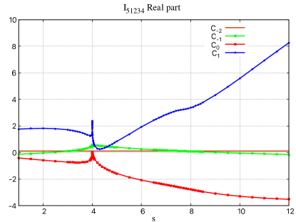
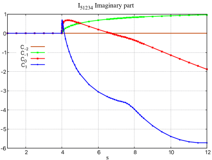
Figure 2: Real and imaginary part of integral ${\mathcal{I}}_{51234}$ as a function of $s$ with DE integrattoin

Finally, graphs are displayed in Figure 2 for the real and imaginary part of the total integral ${\mathcal{I}}_{51234}$ of Eq. (2), where the data were obtained using DE integration and single extrapolation with regard to $\rho$ after an expansion in $\varepsilon$  [17].   

5 Conclusions

Whereas symbolic or symbolic/numerical calculations are performed for some challenging problems using existing software packages, we focus on the development of fully numerical methods for the evaluation of Feynman loop integrals. The integration strategies adhere to black-box approaches for generating an approximation, assuming little or no knowledge of the problem, apart from the specification of the integrand function. We demonstrated efficient strategies based on lattice rules evaluated on GPUs and double-exponential integration, as well as iterated adaptive integration.

We acknowledge the support by JSPS KAKENHI Grant Number JP20K11858, JP20K03941 and JP21K03541, and the National Science Foundation Award Number 1126438 that funded work on multivariate integration.

References

References

- [1] de Doncker E, Yuasa F, Ishikawa T and Kato K 2022 Loop integral computation in the Euclidean or physical kinematical region using numerical integration and extrapolation Proceedings of ACAT 2022 To appear, https://indico.cern.ch/event/1106990/contributions/4997231/
- [2] Nakanishi N 1957 Prog. Theor. Phys. 17 401–418
- [3] Cvitanović P and Kinoshita T 1974 Phys. Rev. D10 3978
- [4] Cvitanović P and Kinoshita T 1974 Phys. Rev. D10 3991
- [5] Cvitanović P and Kinoshita T 1974 Phys. Rev. D10 4007
- [6] Sloan I and Joe S 1994 Lattice Methods for Multiple Integration (Oxford University Press)
- [7] Sidi A 2003 Practical Extrapolation Methods - Theory and Applications (Cambridge Univ. Press) iSBN 0-521-66159-5
- [8] Sidi A 2005 Math. Comp. 75 327–343
- [9] Mori M 1978 Publ. RIMS Kyoto Univ. 14 713–729 https://doi.org/10.2977/prims/1195188835
- [10] Takahasi H and Mori M 1974 Publications of the Research Institute for Mathematical Sciences 9 721–741
- [11] Sugihara M 1997 Numerische Mathematik 75 379–395
- [12] de Doncker E and Yuasa F 2022 Springer Lecture Notes in Computer Science (LNCS) 13378 388–405
- [13] Piessens R, de Doncker E, Überhuber C W and Kahaner D K 1983 QUADPACK, A Subroutine Package for Automatic Integration (Springer Series in Computational Mathematics vol 1) (Springer-Verlag)
- [14] ParInt http://www.cs.wmich.edu/parint
- [15] Olagbemi O E and de Doncker E 2019 Scalable algorithms for multivariate integration with ParAdapt and CUDA Proc. 2019 Int. Conf. on Comp. Science and Comp. Intelligence (IEEE Computer Society) https:doi.org/10.1109/CSCI49370.2019.00093
- [16] de Doncker E, Fujimoto J, Hamaguchi N, Ishikawa T, Kurihara Y, Shimizu Y and Yuasa F 2011 Journal of Computational Science (JoCS) 3 102–112 DOI:10.1016/j.jocs.2011.06.003
- [17] de Doncker E, Ishikawa T, Kato K and Yuasa F 2024 Prog. Theor. Exp. Phys. https://doi.org/10.1093/ptep/ptae122
- [18] Almulihi A and de Doncker E 2017 Accelerating high-dimensional integration using lattice rules on GPUs Proc. 2017 Int. Conf. on Computational Science and Computational Intelligence (CSCI’17) (CPS IEEE)
- [19] Nuyens D and Cools R 2006 Math. Comp. 75 903–920
- [20] Nuyens D and Cools R 2006 Journal of Complexity 22 4–28
- [21] Brezinski C 1980 Numerische Mathematik 35 175–187
- [22] Wynn P 1956 Mathematical Tables and Aids to Computing 10 91–96
- [23] de Doncker E, Fujimoto J, Hamaguchi N, Ishikawa T, Kurihara Y, Ljucovic M, Shimizu Y and Yuasa F 2010 Extrapolation algorithms for infrared divergent integrals arXiv:1110.3587
- [24] de Doncker E, Yuasa F and Kurihara Y 2012 Journal of Physics: Conf. Ser. 368 doi:10.1088/1742-6596/368/1/012060
- [25] Yuasa F, de Doncker E, Ishikawa T, Kato K, Daisaka H and Nakasato N 2022 Numerical method for Feynman integrals: Electroweak high-order correction calculation by DCM IV Fall Meeting of the Physical Society of Japan, 8aA133-6
- [26] Bulirsch R 1964 Numerische Mathematik 6 6–16