Adaptive Multilevel Stochastic Approximation of the Value-at-Risk

Abstract

[13] (CFL23) introduced a multilevel stochastic approximation scheme to compute the value-at-risk of a financial loss that is only simulatable by Monte Carlo. The optimal complexity of the scheme is in $\mathrm{O}(\varepsilon^{-\frac{5}{2}})$, $\varepsilon>0$ being a prescribed accuracy, which is suboptimal when compared to the canonical multilevel Monte Carlo performance. This suboptimality stems from the discontinuity of the Heaviside function involved in the biased stochastic gradient that is recursively evaluated to derive the value-at-risk. To mitigate this issue, this paper proposes and analyzes a multilevel stochastic approximation algorithm that adaptively selects the number of inner samples at each level, and proves that its optimal complexity is in $\mathrm{O}(\varepsilon^{-2}\left|\ln{\varepsilon}\right|^{\frac{5}{2}})$. Our theoretical analysis is exemplified through numerical experiments.

Keywords.  stochastic approximation, value-at-risk, nested Monte Carlo, multilevel Monte Carlo, adaptive Monte Carlo.

MSC. 65C05, 62L20, 62G32, 91Gxx.

Introduction

The value-at-risk (VaR) is the predominant regulatory risk metric in finance [6]. It stands for the quantile, at some confidence level, of the loss on a portfolio. The probability that a loss exceeds the VaR expresses the chances of occurrence of large portfolio losses. Evaluating a portfolio’s VaR is thus paramount to assess its risk. However, a large class of financial portfolios can only be valued by Monte Carlo. This introduces a bias in the loss estimation, thereby increasing the complexity of VaR calculation. Determining a portfolio’s future VaR is thus regarded as a challenging task.

Following the celebrated works on VaR convexification [32, 8, 4], a nascent line of research has adopted a stochastic approximation (SA) viewpoint to estimate the VaR [4, 2, 3, 12, 9]. Recent developments [5, 13, 14] have focused on the nested nature of the problem. Notably, [5] proposes a nested SA (NSA) method that couples an outer SA scheme with an inner nested Monte Carlo scheme to compute the VaR. It is shown in [13] that such a scheme runs optimally in $\mathrm{O}(\varepsilon^{-3})$ time, $\varepsilon>0$ being a prescribed accuracy. Meanwhile, subsequently to the wide success of multilevel Monte Carlo (MLMC) methods [29, 30, 23, 15, 11], multilevel stochastic approximation (MLSA) algorithms [20, 16] have emerged as a means to accelerate biased SA schemes such as NSA. While the latter injects biased nested simulations directly into an iterative SA scheme, MLSA telescopes a sequence of correlated estimate pairs of lower and lower biases, reducing the complexity by an order of magnitude. [13] leverages this multilevel acceleration [20] to reduce the complexity of the VaR NSA scheme of [5] to $\mathrm{O}(\varepsilon^{-2-\delta})$, $\frac{1}{2}\leq\delta<1$ being a small number governed by the integrability degree of the loss. They also identify a parametrization for their MLSA algorithm that achieves a complexity for the estimation of the expected shortfall (ES), a risk measure closely linked to the VaR, in $\mathrm{O}(\varepsilon^{-2}\left|\ln{\varepsilon}\right|^{2})$. [14] further obtains central limit theorems for VaR and ES NSA and MLSA schemes, as well as their Polyak-Ruppert versions that enjoy stronger numerical stability properties.

Albeit significant, the performance gain achieved by MLSA over NSA in estimating the VaR [13] is to be nuanced. The canonical optimal complexity for multilevel techniques is of order $\varepsilon^{-2}$ [23, 20]. The suboptimality of the VaR MLSA scheme arises from its inner recursions relying on the evaluation of a discontinuous gradient that is similar to a Heaviside ($x\mapsto\mathds{1}_{x>0}$). When a biased simulation of the loss falls on the opposite side of the discontinuity relative to the exact target loss, the multilevel recursion incurs an $\mathrm{O}(1)$ update error. The accumulation of these errors propagates to the final estimator, leading to the suboptimality.

Motivated by valuing a digital option with Heaviside payoff in a local volatility model, [22] surveys multiple approaches to the above discontinuity issue in a multilevel Monte Carlo (MLMC) context. Most techniques described therein emanate from the derivative sensitivity computation literature and their common goal is to lower the variance of the paired estimators at each level of the multilevel simulation. We retain three ideas that may apply to our nested SA setting. Firstly, a natural idea is to smoothen the Heaviside payoff, but this only attains a complexity in $\mathrm{O}(\varepsilon^{-2-\frac{1}{4}})$ due to a large smoothing Lipschitz constant. Secondly, Malliavin calculus could be used in conjunction with a cubic spline interpolation, which however propagates regression noises to the final estimator. Finally, levelwise adaptive refinement of inner Monte Carlo samplings seems to be a versatile technique that achieves the desired performance gain. It advocates to dynamically refine the biased simulations in order to deal with the discontinuity issue [24, 28, 25]. We quickly overview this technique below.

An early example of adaptive nested Monte Carlo simulation can be traced back to [10], who endeavor to accelerate the nested Monte Carlo root-finding algorithm of [27] for approximating the VaR. The latter algorithm combines an outer bisection method with an inner Monte Carlo sampling of the probability that the loss exceed the VaR, and involves the evaluation of a Heaviside centered at the VaR itself. Such a method proves however to be computationally more demanding than the aforementioned SA approaches. The adaptive strategy of [10] involves refining simulations for risk scenarios that are too close to the VaR, thereby reducing their probability of falling on the wrong side of the VaR threshold. Evaluating the Heaviside function at the biased loss becomes almost equivalent to evaluating it at the true loss. [24] revisits the same concept as [10], extending their method to the nested MLMC paradigm by adapting the number of inner simulations at each level. [28] generalizes this methodology to a broader class of MLMC problems.

[17] has led to similar adaptive ideas in a partial differential equation Monte Carlo approximation setting, where the Monte Carlo estimation error is assumed to be almost surely bounded. Note that the terminology “adaptive MLMC” has also been employed in different meanings, for adaptive path simulation [31] and importance sampling [7].

In this article, we develop an adaptive refinement strategy to efficiently estimate the VaR using the MLSA algorithm derived in [13]. As in MLMC, our adaptive strategy prioritizes aligning the innovations with their target samplings relative to the discontinuities of the update functions at the SA iterates. However, the strategy that was developed for Monte Carlo in [24, 28] does not directly apply to our SA setting, since refining the innovations that drive an SA scheme shifts their distributions relatively to the SA iterates, which themselves evolve from one recursion to the next. On the one hand, this increases the risk of steering the iterates away from the target VaR. On the other hand, it affects the original SA problem formulation, rendering it possibly non-convex and possessing multiple stationary points. To address this issue, we carefully incorporate a saturation factor, varying throughout the iterations, to prevent the potential deviation of the iterates from the target VaR.

We apply our strategy to both NSA and MLSA paradigms and provide sharp $L^{2}(\mathbb{P})$-controls. For a prescribed accuracy $\varepsilon>0$, their optimal complexities are shown to be $\mathrm{O}(\varepsilon^{-\frac{5}{2}}\left|\ln{\varepsilon}\right|^{\frac{1}{2}})$ and $\mathrm{O}(\varepsilon^{-2}\left|\ln{\varepsilon}\right|^{\frac{5}{2}})$ respectively, resulting in an order of magnitude $\varepsilon^{\frac{1}{2}}$ speed-up on their non-adaptive counterparts, up to a logarithmic factor. The adaptive MLSA algorithm largely attains a comparable complexity order to the standard unbiased Robbins-Monro algorithm, thus demonstrating the narrowing of the performance gap between nested MLSA schemes and Robbins-Monro schemes in the context of Heaviside-type update functions. Our numerical analyses, conducted on a toy model as well as a more concrete financial setup, strongly support our theoretical findings.

The paper is structured as follows. Section 1 recalls the problem and main results in [13] regarding the estimation of the VaR using MLSA. Section 2 develops an adaptive refinement strategy to enhance the efficiency of the Monte Carlo sampling that is nested within the MLSA approach. Sections 3 and 4 exploit this strategy to reduce the complexities of NSA and MLSA and provide subsequent $L^{2}(\mathbb{P})$-controls and complexity rates. Section 5 presents numerical studies to demonstrate the performance improvement resulting from the adaptive strategy.

1 Stochastic Approximation Approach

This section recalls the setting and main results in [13] on the stochastic approximation of the VaR. They will serve as a baseline for the adaptive strategy that we develop in Section 2.

1.1 Unbiased Stochastic Approximation Algorithm

Let $(\Omega,\mathcal{F},\mathbb{P})$ be a probability space accommodating all of the subsequent random variables. Let $X_{0}\in L^{1}(\mathbb{P})$ be an $\mathbb{R}$-valued random loss of a portfolio, defined at some time horizon $\tau>0$. Following [1, 19], the VaR of $X_{0}$ at some confidence level $\alpha\in(0,1)$, denoted $\xi^{0}_{\star}$, is defined as

$$\xi^{0}_{\star}\coloneqq\inf{\big{\{}\xi\in\mathbb{R}\colon\mathbb{P}(X_{0}\leq\xi)\geq\alpha\big{\}}}.$$ (1.1)

As stated in [32, 8, 4], if the cdf $F_{X_{0}}$ of $X_{0}$ is continuous, then $\xi^{0}_{\star}$ is the left-end solution to

$$\operatorname*{argmin}_{\xi\in\mathbb{R}}{V_{0}(\xi)},\quad\mbox{ where }\quad V_{0}(\xi)\coloneqq\xi+\frac{1}{1-\alpha}\mathbb{E}[(X_{0}-\xi)^{+}].$$ (1.2)

Moreover, $V_{0}$ is convex and continuously differentiable on $\mathbb{R}$, with $V_{0}^{\prime}(\xi)=\frac{1}{1-\alpha}(F_{X_{0}}(\xi)-\alpha)=\mathbb{E}[H(\xi,X_{0})]$, $\xi\in\mathbb{R}$, where

$$H(\xi,x)=1-\frac{1}{1-\alpha}\mathds{1}_{x\geq\xi},\quad\xi,x\in\mathbb{R}.$$ (1.3)

If $F_{X_{0}}$ is additionally increasing, then $V_{0}$ is strictly convex and $\xi^{0}_{\star}$ is the unique minimizer of $V_{0}$:

$$\xi^{0}_{\star}=\operatorname*{argmin}{V_{0}}.$$ (1.4)

Besides, if $X_{0}$ admits a continuous pdf $f_{X_{0}}$, then $V_{0}$ is twice continuously differentiable on $\mathbb{R}$, with $V_{0}^{\prime\prime}(\xi)=\frac{1}{1-\alpha}f_{X_{0}}(\xi)$, $\xi\in\mathbb{R}$.

When iid samples of $X_{0}$ are available, [4] proposes to estimate $\xi^{0}_{\star}$ using the unbiased SA scheme of dynamics

$$\xi^{0}_{n+1}=\xi^{0}_{n}-\gamma_{n+1}H(\xi^{0}_{n},X_{0}^{(n+1)}),\quad n\in\mathbb{N},$$ (SA)

where $(X_{0}^{(n)})_{n\geq 1}\stackrel{{\scriptstyle\text{\tiny\rm iid}}}{{\sim}}X_{0}$, $\xi^{0}_{0}$ is a real-valued random initialization independent of the innovations $(X_{0}^{(n)})_{n\geq 1}$, and $(\gamma_{n})_{n\geq 1}$ is a positive non-increasing sequence such that $\sum_{n\geq 1}\gamma_{n}=\infty$ and $\lim_{n\to\infty}\gamma_{n}=0$.

We are interested in the setting where $X_{0}$ writes as a conditional expectation:

$$X_{0}=\mathbb{E}[\varphi(Y,Z)|Y].$$ (1.5)

Here, $Y$ and $Z$ are two independent random variables taking values in $\mathbb{R}^{d}$ and $\mathbb{R}^{q}$ respectively, and $\varphi\colon\mathbb{R}^{d}\times\mathbb{R}^{q}\to\mathbb{R}$ is a measurable function such that $\varphi(Y,Z)\in L^{1}(\mathbb{P})$. From a financial standpoint, $Y$ typically models the dynamics of the portfolio’s risk factors up to the time horizon $\tau$ of the loss, $Z$ their dynamics beyond $\tau$ and $\varphi(Y,Z)$ the subsequent future cash flows. Generally, the risk factors $Y$ and $Z$ can be sampled from a model and the cash flow structure $\varphi$ is known.

In the case that $X_{0}$ cannot be sampled exactly, one must leverage its nested formulation to produce suitable simulations for the SA approach.

1.2 Nested Stochastic Approximation Algorithm

Let $\mathbb{N}_{0}\coloneqq\mathbb{N}\setminus\{0\}$. A natural idea is to approximate $X_{0}$ by the nested Monte Carlo estimator

$$X_{h}\coloneqq\frac{1}{K}\sum_{k=1}^{K}\varphi(Y,Z^{(k)}),\quad\mbox{ where }\quad h\coloneqq\frac{1}{K}\in\mathcal{H}=\Big{\{}\frac{1}{K^{\prime}},K^{\prime}\in\mathbb{N}_{0}\Big{\}}$$ (1.6)

and $Y$ and $(Z^{(k)})_{1\leq k\leq K}\stackrel{{\scriptstyle\text{\tiny\rm iid}}}{{\sim}}Z$ are independent. $h$ is termed the bias parameter since it helps control the VaR estimation bias as we clarify next. We swap $X_{0}$ by $X_{h}$, $h\in\mathcal{H}$, in the original problem (1.2) and obtain the approximate problem

$$\operatorname*{argmin}_{\xi\in\mathbb{R}}{V_{h}(\xi)},\quad\mbox{ where }\quad V_{h}(\xi)\coloneqq\xi+\frac{1}{1-\alpha}\mathbb{E}[(X_{h}-\xi)^{+}].$$ (1.7)

Again, assuming that $\varphi(Y,Z)\in L^{1}(\mathbb{P})$, if the cdf $F_{X_{h}}$ of $X_{h}$ is continuous, then $V_{h}$ is convex and continuously differentiable on $\mathbb{R}$, with $V_{h}^{\prime}(\xi)=\frac{1}{1-\alpha}(F_{X_{h}}(\xi)-\alpha)=\mathbb{E}[H(\xi,X_{h})]$, $\xi\in\mathbb{R}$, recalling the definition (1.3). If $F_{X_{h}}$ is additionally increasing, then $V_{h}$ is strictly convex and

$$\xi^{h}_{\star}=\operatorname*{argmin}{V_{h}}$$ (1.8)

is well defined and constitutes a biased estimator of $\xi^{0}_{\star}$. Finally, If $X_{h}$ admits a continuous pdf $f_{X_{h}}$, then $V_{h}$ is twice continuously differentiable on $\mathbb{R}$, with $V_{h}^{\prime\prime}(\xi)=(1-\alpha)^{-1}f_{X_{h}}(\xi)$, $\xi\in\mathbb{R}$.

Assuming $F_{X_{h}}$ continuous and increasing, $\xi^{0}_{\star}$ can be estimated with a bias $h\in\mathcal{H}$ using the NSA scheme of dynamics

$$\xi^{h}_{n+1}=\xi^{h}_{n}-\gamma_{n+1}H(\xi^{h}_{n},X_{h}^{(n+1)}),\quad n\in\mathbb{N},$$ (NSA)

where $(X_{h}^{(n)})_{n\geq 1}\stackrel{{\scriptstyle\text{\tiny\rm iid}}}{{\sim}}X_{h}$, $\xi^{h}_{0}$ is a real-valued random initialization independent of the innovations $(X_{h}^{(n)})_{n\geq 1}$ and $(\gamma_{n})_{n\geq 1}$ is a positive non-increasing sequence such that $\sum_{n\geq 1}\gamma_{n}=\infty$ and $\lim_{n\to\infty}\gamma_{n}=0$.

Convergence Analysis.

Let $\overline{\mathcal{H}}\coloneqq\mathcal{H}\cup\{0\}$. The global error of (NSA) writes as a sum of a statistical and a bias errors:

$$\xi^{h}_{n}-\xi^{0}_{\star}=\big{(}\xi^{h}_{n}-\xi^{h}_{\star}\big{)}+(\xi^{h}_{\star}-\xi^{0}_{\star}),$$ (1.9)

Assumption 1.1 ([13, Assumptions 2.2 & 2.5]).

1. For any $h\in\mathcal{H}$, $F_{X_{h}}$ admits the first order Taylor expansion

   $$F_{X_{h}}(\xi)-F_{X_{0}}(\xi)=v(\xi)h+w(\xi,h)h,\quad\xi\in\mathbb{R},$$

   for some functions $v,w(\,\cdot\,,h)\colon\mathbb{R}\to\mathbb{R}$ satisfying, for any $\xi^{0}_{\star}\in\operatorname*{Argmin}{V_{0}}$,

   $$\int^{\infty}_{\xi^{0}_{\star}}v(\xi)\mathrm{d}\xi<\infty,\qquad\lim_{\mathcal{H}\ni h\downarrow 0}w(\xi^{0}_{\star},h)=\lim_{\mathcal{H}\ni h\downarrow 0}\int^{\infty}_{\xi^{0}_{\star}}w(\xi,h)\mathrm{d}\xi=0.$$

2. For any $h\in\overline{\mathcal{H}}$, the law of $X_{h}$ admits a continuous pdf $f_{X_{h}}$ with respect to the Lebesgue measure. Moreover, the pdfs $(f_{X_{h}})_{h\in\mathcal{H}}$ converge locally uniformly to $f_{X_{0}}$.

3. For any $R>0$,

   $$\inf_{h\in\overline{\mathcal{H}},\,\xi\in B(\xi^{0}_{\star},R)}{f_{X_{h}}(\xi)}>0.$$

4. The pdfs $(f_{X_{h}})_{h\in\overline{\mathcal{H}}}$ are uniformly bounded and uniformly Lipschitz, namely,

   $$\sup_{h\in\overline{\mathcal{H}}}{(\|f_{X_{h}}\|_{\infty}+[f_{X_{h}}]_{\text{\rm Lip}})}<\infty,$$

   where $[f_{X_{h}}]_{\text{\rm Lip}}$ denotes the Lipschitz constant of $f_{X_{h}}$, $h\in\overline{\mathcal{H}}$.

Remark 1.1 ([14, Remark 1.1]).

[26, Propositions 5.1(a,​​b)] guarantee Assumptions 1.1(i,ii). The last part of Assumption 1.1(i) reads $w(\xi^{0}_{\star},h)=\int_{\xi^{0}_{\star}}^{\infty}w(\xi,h)\mathrm{d}\xi=\mathrm{o}(1)$ as $\mathcal{H}\ni h\downarrow 0$, $\xi^{0}_{\star}\in\operatorname*{Argmin}{V_{0}}$. Assumptions 1.1(iii,iv) are natural in view of Assumption 1.1(ii) and the increasing nature of $F_{X_{0}}$. By Assumptions 1.1(ii,iii), for any $h\in\overline{\mathcal{H}}$ and any $\xi^{h}_{\star}\in\operatorname*{Argmin}{V_{h}}$, $V_{h}^{\prime\prime}(\xi^{h}_{\star})=(1-\alpha)^{-1}f_{X_{h}}(\xi^{h}_{\star})>0$, subsequently reducing $\operatorname*{Argmin}{V_{h}}$ to a singleton $\{\xi^{h}_{\star}\}$.

For any positive integer $q$, we let

$$\bar{\lambda}_{q}\coloneqq\inf_{h\in\overline{\mathcal{H}}}{\bar{\lambda}_{h,q}},$$ (1.10)

where $(\bar{\lambda}_{h,q})_{h\in\overline{\mathcal{H}},q\geq 1}$ are defined in Lemma A.2(iii).

Lemma 1.2 ([13, Proposition 2.4 & Theorem 2.7(i)]).

1. Suppose that $\varphi(Y,Z)\in L^{1}(\mathbb{P})$, that Assumptions 1.1(i,ii) hold, and that the pdf $f_{X_{0}}$ is positive. Then, as $\mathcal{H}\ni h\downarrow 0$, for any $\xi^{h}_{\star}\in\operatorname*{Argmin}{V_{h}}$,

   $$\xi^{h}_{\star}-\xi^{0}_{\star}=-\frac{v(\xi^{0}_{\star})}{f_{X_{0}}(\xi^{0}_{\star})}h+\mathrm{o}(h).$$

2. Suppose that $\varphi(Y,Z)\in L^{2}(\mathbb{P})$, that Assumption 1.1 holds, and that

   $$\sup_{h\in\overline{\mathcal{H}}}{\mathbb{E}\Big{[}|\xi^{h}_{0}|^{2}\exp\Big{(}\frac{4}{1-\alpha}k_{\alpha}\sup_{h\in\overline{\mathcal{H}}}\|f_{X_{h}}\|_{\infty}|\xi_{0}^{h}|\Big{)}\Big{]}}<\infty,$$ (1.11)

   where $k_{\alpha}=1\vee\frac{\alpha}{1-\alpha}$. If $\gamma_{n}=\gamma_{1}n^{-\beta}$, $\beta\in(0,1]$, with $\bar{\lambda}_{1}\gamma_{1}>1$ if $\beta=1$, then there exists a positive constant $C<\infty$ such that, for any positive integer $n$,

   $$\sup_{h\in\mathcal{H}}\mathbb{E}[(\xi^{h}_{n}-\xi^{h}_{\star})^{2}]\leq C\gamma_{n}.$$

Complexity Analysis.

The controls of Lemma 1.2 on the bias and statistical errors in (1.9) result in the following complexities.

Proposition 1.3 ([13, Theorem 2.8]).

Let $\varepsilon\in(0,1)$ be a prescribed accuracy. Within the framework of Lemma 1.2(ii), setting

$$h=\frac{1}{\lceil\varepsilon^{-1}\rceil}\sim\varepsilon\quad\mbox{ and }\quad n=\big{\lceil}\varepsilon^{-\frac{2}{\beta}}\big{\rceil}$$

yields a global $L^{1}(\mathbb{P})$ error for (NSA) of order $\varepsilon$ as $\varepsilon\downarrow 0$. The corresponding computational cost satisfies

$$\operatorname{Cost}^{\beta}_{\text{\tiny\rm NSA}}\leq Cnh^{-1}\sim C\varepsilon^{-\frac{2}{\beta}-1}\quad\mbox{ as }\quad\varepsilon\downarrow 0,$$

for some positive constant $C<\infty$ independent of $\varepsilon$. The minimal computational cost satisfies

$$\operatorname{Cost}^{1}_{\text{\tiny\rm NSA}}\leq C\varepsilon^{-3}\quad\mbox{ as }\quad\varepsilon\downarrow 0,$$

and is attained for $\gamma_{n}=\gamma_{1}n^{-1}$, i.e. for $\beta=1$ under the constraint $\bar{\lambda}_{1}\gamma_{1}>1$.

1.3 Multilevel Stochastic Approximation Algorithm

With a complexity ceiling for nested VaR estimation at $\mathrm{O}(\varepsilon^{-3})$ as achieved by (NSA), a multilevel approach is proposed in [13] to accelerate the latter scheme. We recall below the MLSA scheme and the associated $L^{2}(\mathbb{P})$-control and complexity.

Take $h_{0}\coloneqq\frac{1}{K}\in\mathcal{H}$, $M\geq 2$ an integer and $L\in\mathbb{N}_{0}$ a number of levels, and let

$$h_{\ell}\coloneqq\frac{h_{0}}{M^{\ell}}=\frac{1}{KM^{\ell}}\in\mathcal{H},\quad\ell=0,\dots,L.$$ (1.12)

To each bias parameter $h_{\ell}$, $\ell=0,\dots,L$, corresponds an approximate problem $\operatorname*{argmin}_{\xi\in\mathbb{R}}{V_{h_{\ell}}(\xi)}$ to (1.2) of unique solution $\xi^{h_{\ell}}_{\star}$. These solutions can be telescoped into

$$\xi^{h_{L}}_{\star}=\xi^{h_{0}}_{\star}+\sum_{\ell=1}^{L}\xi^{h_{\ell}}_{\star}-\xi^{h_{\ell-1}}_{\star}.$$ (1.13)

By denoting $\mathbf{N}\coloneqq(N_{\ell})_{0\leq\ell\leq L}$ a sequence of iterations amounts, the multilevel SA scheme [13, 20] consists in approximating $\xi^{0}_{\star}\approx\xi^{h_{L}}_{\star}$ with

$$\xi^{\text{\tiny\rm ML}}_{\mathbf{N}}=\xi^{h_{0}}_{N_{0}}+\sum_{\ell=1}^{L}\xi^{h_{\ell}}_{N_{\ell}}-\xi^{h_{\ell-1}}_{N_{\ell}},$$ (MLSA)

where each level $\ell=0,\dots,L$ is simulated independently. More precisely, once $\xi^{h_{0}}_{N_{0}}$ is simulated using $N_{0}$ iterations of (NSA) with bias $h_{0}$, at each level $\ell=1,\dots,L$, for $j\in\{(\ell-1),\ell\}$, $\xi^{h_{j}}_{N_{\ell}}$ is obtained by iterating

$$\xi^{h_{j}}_{n+1}=\xi^{h_{j}}_{n}-\gamma_{n+1}H(\xi^{h_{j}}_{n},X_{h_{j}}^{(n+1)}),\quad n\in\{0,\dots,N_{\ell}-1\},$$ (1.14)

where $(X_{h_{\ell-1}}^{(n)},X_{h_{\ell}}^{(n)})_{1\leq n\leq N_{\ell}}\stackrel{{\scriptstyle\text{\tiny\rm iid}}}{{\sim}}(X_{h_{\ell-1}},X_{h_{\ell}})$ and $\xi^{h_{\ell-1}}_{0}$ and $\xi^{h_{\ell}}_{0}$ are real-valued random initializations independent of the innovations $(X_{h_{\ell-1}}^{(n)},X_{h_{\ell}}^{(n)})_{1\leq n\leq N_{\ell}}$. Crucially, at each level $\ell\in\{1,\dots,L\}$, $X_{h_{\ell}}$ and $X_{h_{\ell-1}}$ are perfectly correlated, in the sense that

$$X_{h_{\ell-1}}=\frac{1}{KM^{\ell-1}}\sum_{k=1}^{KM^{\ell-1}}\varphi(Y,Z^{(k)}),\quad X_{h_{\ell}}=\frac{1}{M}X_{h_{\ell-1}}+\frac{1}{KM^{\ell}}\sum_{k=KM^{\ell-1}+1}^{KM^{\ell}}\varphi(Y,Z^{(k)}),$$ (1.15)

where $(Z^{(k)})_{1\leq k\leq KM^{\ell}}\stackrel{{\scriptstyle\text{\rm\tiny iid}}}{{\sim}}Z$ are independent of $Y$.

At each level $\ell=1,\dots,L$, $\xi^{h_{\ell}}_{N_{\ell}}$ and $\xi^{h_{\ell-1}}_{N_{\ell}}$ are referred to as the fine and coarse approximations. $\xi^{h_{0}}_{N_{0}}$ is referred to as the initial (or level $0$) approximation. We can infer from (1.14) that (MLSA) correlates multiple (NSA) pairs, each pair being set with consecutive bias parameters on the geometric scale $\mathcal{H}_{0}\coloneqq\{h_{\ell},\ell\geq 0\}$. The produced effect is an incremental bias correction of the level $0$ approximation of bias $h_{0}$. Conversely, (NSA) can be viewed as an (MLSA) instance with $0$ (higher) levels.

Convergence Analysis.

The following lemma delimits three frameworks under which we later derive $L^{2}(\mathbb{P})$-controls and complexities for (MLSA).

Lemma 1.4 ([13, Proposition 3.2]).

1. Assume that the real-valued random variables $X_{h}$ admit pdfs $f_{X_{h}}$ that are bounded uniformly in $h\in\overline{\mathcal{H}}$.

   1. If

      $$\mathbb{E}\big{[}\big{|}\varphi(Y,Z)-\mathbb{E}[\varphi(Y,Z)|Y]\big{|}^{p_{\star}}\big{]}<\infty\quad\mbox{for some $p_{\star}>1$},$$ (1.16)

      then, for any $h,h^{\prime}\in\overline{\mathcal{H}}$ such that $0\leq h\leq h^{\prime}$ and any $\xi\in\mathbb{R}$,

      $$\mathbb{E}\big{[}\big{|}\mathds{1}_{X_{h}>\xi}-\mathds{1}_{X_{h^{\prime}}>\xi}\big{|}\big{]}\leq C(h^{\prime}-h)^{\frac{p_{\star}}{2(p_{\star}+1)}},$$

      where $C\coloneqq B_{p_{\star}}\mathbb{E}\big{[}\big{|}\varphi(Y,Z)-\mathbb{E}[\varphi(Y,Z)|Y]\big{|}^{p_{\star}}\big{]}^{\frac{1}{p_{\star}+1}}(\sup_{h\in\overline{\mathcal{H}}}\|f_{X_{h}}\|_{\infty})^{\frac{p_{\star}}{p_{\star}+1}}$, with $B_{p_{\star}}$ a positive constant that depends only upon $p_{\star}$.

   2. Assume that there exists a non-negative constant $C_{g}<\infty$ such that, for all $u\in\mathbb{R}$,

      $$\mathbb{E}\big{[}\exp\big{(}u\big{(}\varphi(Y,Z)-\mathbb{E}[\varphi(Y,Z)|Y]\big{)}\big{)}\big{|}Y\big{]}\leq\mathrm{e}^{C_{g}u^{2}}\quad\mathbb{P}\text{\rm-as}.$$ (1.17)

      Then, for any $h,h^{\prime}\in\overline{\mathcal{H}}$ such that $0\leq h<h^{\prime}$ and any $\xi\in\mathbb{R}$,

      $$\mathbb{E}\big{[}\big{|}\mathds{1}_{X_{h}>\xi}-\mathds{1}_{X_{h^{\prime}}>\xi}\big{|}\big{]}\leq 2\sqrt{C_{g}(h^{\prime}-h)}\Big{(}1+\sup_{h^{\prime\prime}\in\overline{\mathcal{H}}}\|f_{X_{h^{\prime\prime}}}\|_{\infty}\sqrt{2\left|\ln\big{(C_{g}(h^{\prime}-h)\big{)}}\right|}\Big{)}.$$

2. Let $G_{\ell}\coloneqq h_{\ell}^{-\frac{1}{2}}(X_{h_{\ell}}-X_{h_{\ell-1}})$, define $F_{X_{h_{\ell-1}}\,|\,G_{\ell}=g}\colon x\mapsto\mathbb{P}(X_{h_{\ell-1}}\leq x\,|\,G_{\ell}=g)$, $g\in\mathrm{supp}(\mathbb{P}_{G_{\ell}})$, $\ell\geq 1$, and consider the sequence of random variables $(K_{\ell})_{\ell\geq 1}$ given by $K_{\ell}\coloneqq K_{\ell}(G_{\ell})$, where

   $$K_{\ell}(g)\coloneqq\sup_{x\neq y}\,\frac{\big{|}F_{X_{h_{\ell-1}}\,|\,G_{\ell}=g}(x)-F_{X_{h_{\ell-1}}\,|\,G_{\ell}=g}(y)\big{|}}{|x-y|},\quad\ell\geq 1,g\in\mathrm{supp}(\mathbb{P}_{G_{\ell}}).$$

   Assume that $(K_{\ell})_{\ell\geq 1}$ satisfies

   $$\sup_{\ell\geq 1}\,\mathbb{E}[|G_{\ell}|K_{\ell}]<\infty.$$ (1.18)

   Then,

   $$\sup_{\ell\geq 1,\xi\in\mathbb{R}}\,h_{\ell}^{-\frac{1}{2}}\mathbb{E}\big{[}\big{|}\mathds{1}_{X_{h_{\ell}}>\xi}-\mathds{1}_{X_{h_{\ell-1}}>\xi}\big{|}\big{]}<\infty.$$

Remark 1.2 ([13, Remark 3.3]).

Lemma 1.4’s frameworks are ordered by strength. The Gaussian concentration framework (1.17) holds if $\mathbb{E}[\exp(u_{0}\varphi(Y,Z)^{2})|Y]$ is bounded for some $u_{0}>0$ [21, 18]. It entails (1.16) for any $p_{\star}>1$ via an exponential series expansion. The framework (1.18) relaxes [27, Assumption 1] and is computationally optimal (c.f. Proposition 1.7(iii)). It holds for instance if $F_{X_{h_{\ell-1}}\,|\,G_{\ell}=g}$ is uniformly Lipschitz in $g$ and $\ell$.

Assumption 1.5 ([13, Assumption 3.4]).

There exist positive constants $C,\delta_{0}<\infty$ such that, for any $h\in\mathcal{H}$ and any compact set $\mathcal{K}\subset\mathbb{R}$,

$$\sup_{\xi\in\mathcal{K}}{|f_{X_{h}}(\xi)-f_{X_{0}}(\xi)|}\leq Ch^{\frac{1}{4}+\delta_{0}}.$$

Remark 1.3 ([13, Remark 3.5]).

Assumption 1.5 holds within the framework of [26, Proposition 5.1(a)].

Theorem 1.6 ([13, Theorem 3.6]).

Suppose that $\varphi(Y,Z)\in L^{2}(\mathbb{P})$, that Assumptions 1.1 and 1.5 hold, and that

$$\sup_{h\in\overline{\mathcal{H}}}{\mathbb{E}\Big{[}|\xi^{h}_{0}|^{4}\exp\Big{(}\frac{16}{1-\alpha}k_{\alpha}\sup_{h\in\overline{\mathcal{H}}}\|f_{X_{h}}\|_{\infty}|\xi_{0}^{h}|\Big{)}\Big{]}}<\infty.$$

Within the frameworks of Lemma 1.4, if $\gamma_{n}=\gamma_{1}n^{-\beta}$, $\beta\in(0,1]$, with $\bar{\lambda}_{2}\gamma_{1}>2$ if $\beta=1$, then, there exists some constant $K<\infty$ such that, for any positive integer $L$ and any $\mathbf{N}=(N_{0},\dots,N_{L})\in\mathbb{N}_{0}^{L+1}$,

$$\mathbb{E}\big{[}\big{(}\xi^{\text{\tiny\rm ML}}_{\mathbf{N}}-\xi_{\star}^{h_{L}}\big{)}^{2}\big{]}\leq K\bigg{(}\gamma_{N_{0}}+\bigg{(}\sum_{\ell=1}^{L}\gamma_{N_{\ell}}\bigg{)}^{2}+\sum_{\ell=1}^{L}\gamma_{N_{\ell}}^{\frac{3}{2}}+\sum_{\ell=1}^{L}\gamma_{N_{\ell}}\epsilon(h_{\ell})\bigg{)},$$ (1.19)

where

$$\epsilon(h)\coloneqq\begin{cases}h^{\frac{p_{*}}{2(1+p_{*})}}&\text{if\leavevmode\nobreak\ \eqref{assumption:finite:Lp:moment} holds,}\\ h^{\frac{1}{2}}\left|\ln{h_{\ell}}\right|^{\frac{1}{2}}&\text{if\leavevmode\nobreak\ \eqref{assumption:conditional:gaussian:concentration} holds,}\\ h^{\frac{1}{2}}&\text{if\leavevmode\nobreak\ \eqref{assump:unif:lipschitz:integrability:conditional:cdf} holds,}\end{cases}\quad h\in\mathcal{H}.$$ (1.20)

Complexity Analysis.

The global error of (MLSA) can be decomposed into a statistical and a bias errors:

$$\xi^{\text{\tiny ML}}_{\mathbf{N}}-\xi^{0}_{\star}=\big{(}\xi^{\text{\tiny ML}}_{\mathbf{N}}-\xi^{h_{L}}_{\star}\big{)}+(\xi^{h_{L}}_{\star}-\xi^{0}_{\star}).$$ (1.21)

Proposition 1.7 ([13, Proposition 3.7, Lemma 3.8 & Theorem 3.9]).

1. Suppose that Assumption 1.1(i) is satisfied. Let $\varepsilon\in(0,1)$ be a prescribed accuracy. If $h_{0}>\varepsilon$, then, setting

   $$L=\bigg{\lceil}\frac{\ln{h_{0}\varepsilon^{-1}}}{\ln{M}}\bigg{\rceil}$$ (1.22)

   achieves a bias error for (MLSA) of order $\varepsilon$.

2. The computational cost of (MLSA) satisfies

   $$\operatorname{Cost}_{\text{\tiny\rm MLSA}}^{\beta}\leq C\sum_{\ell=0}^{L}\frac{N_{\ell}}{h_{\ell}},$$

   for some positive constant $C<\infty$.

3. Let $\varepsilon\in(0,1)$ be a prescribed accuracy. Within the framework of Theorem 1.6, setting

   $$N_{\ell}=\bigg{\lceil}(K\gamma_{1})^{\frac{1}{\beta}}\varepsilon^{-\frac{2}{\beta}}\bigg{(}\sum_{\ell^{\prime}=0}^{L}h_{\ell^{\prime}}^{-\frac{\beta}{1+\beta}}\epsilon(h_{\ell^{\prime}})^{\frac{1}{1+\beta}}\bigg{)}^{\frac{1}{\beta}}h_{\ell}^{\frac{1}{1+\beta}}\epsilon(h_{\ell})^{\frac{1}{1+\beta}}\bigg{\rceil},\quad\ell=0,\dots,L,$$

   i.e.

   $$N_{\ell}=\begin{cases}\Big{\lceil}(K\gamma_{1})^{\frac{1}{\beta}}\varepsilon^{-\frac{2}{\beta}}h_{\ell}^{\frac{1}{1+\beta}(1+\frac{p_{*}}{2(1+p_{*})})}\Big{(}\sum_{\ell^{\prime}=0}^{L}h_{\ell^{\prime}}^{\frac{1}{1+\beta}(-\beta+\frac{p_{*}}{2(1+p_{*})})}\Big{)}^{\frac{1}{\beta}}\Big{\rceil}&\text{if\leavevmode\nobreak\ \eqref{assumption:finite:Lp:moment} holds,}\\ \Big{\lceil}(K\gamma_{1})^{\frac{1}{\beta}}\varepsilon^{-\frac{2}{\beta}}h_{\ell}^{\frac{3}{2(1+\beta)}}\left|\ln{h_{\ell}}\right|^{\frac{1}{2(1+\beta)}}\Big{(}\sum_{\ell^{\prime}=0}^{L}h_{\ell^{\prime}}^{\frac{1-2\beta}{2(1+\beta)}}\left|\ln{h_{\ell^{\prime}}}\right|^{\frac{1}{2(1+\beta)}}\Big{)}^{\frac{1}{\beta}}\Big{\rceil}&\text{if\leavevmode\nobreak\ \eqref{assumption:conditional:gaussian:concentration} holds,}\\ \Big{\lceil}(K\gamma_{1})^{\frac{1}{\beta}}\varepsilon^{-\frac{2}{\beta}}h_{\ell}^{\frac{3}{2(1+\beta)}}\Big{(}\sum_{\ell^{\prime}=0}^{L}h_{\ell^{\prime}}^{\frac{1-2\beta}{2(1+\beta)}}\Big{)}^{\frac{1}{\beta}}\Big{\rceil}&\text{if\leavevmode\nobreak\ \eqref{assump:unif:lipschitz:integrability:conditional:cdf} holds,}\end{cases}$$

   where $K$ is the constant on the right hand side of (1.19), achieves a statistical error on the estimation of $\xi^{0}_{\star}$ of order $\varepsilon$. The optimal computational cost is attained when $\beta=1$ under the constraint $\bar{\lambda}_{2}\gamma_{1}>2$, in which case

   $$\operatorname{Cost}_{\text{\tiny\rm MLSA}}^{1}\leq C\begin{cases}\varepsilon^{-3+\frac{p_{*}}{2(1+p_{*})}}&\text{if\leavevmode\nobreak\ \eqref{assumption:finite:Lp:moment} holds,}\\ \varepsilon^{-\frac{5}{2}}\left|\ln{\varepsilon}\right|^{\frac{1}{2}}&\text{if\leavevmode\nobreak\ \eqref{assumption:conditional:gaussian:concentration} holds,}\\ \varepsilon^{-\frac{5}{2}}&\text{if\leavevmode\nobreak\ \eqref{assump:unif:lipschitz:integrability:conditional:cdf} holds.}\end{cases}$$

Remark 1.4.

The advantageous framework described by (1.18) results in an optimal computational cost in $\mathrm{O}(\varepsilon^{-\frac{5}{2}})$, which remains suboptimal compared to the canonical optimum of $\mathrm{O}(\varepsilon^{-2})$ that is achievable by multilevel techniques [23, 20].

The next section devises a strategy to adaptively refine the inner Monte Carlo innovations of (NSA) and (MLSA).

2 Adaptive Refinement Strategy

The suboptimality of (MLSA) is linked to the discontinuity of the gradient $H$ (1.3) intervening in the VaR recursion (1.14). Indeed, for $n\in\mathbb{N}_{0}$, if the simulated loss

$$X_{h}^{(n)}=\frac{1}{K}\sum_{k=1}^{K}\varphi(Y^{(n)},Z^{(k,n)})$$

is too close to the estimate $\xi^{h}_{n-1}$ but falls on the opposite side of the discontinuity of $H(\xi^{h}_{n-1},\,\cdot\,)$ with respect to its sampling target

$$X_{0}^{(n)}\coloneqq\mathbb{E}[\varphi(y,Z)]_{|y=Y^{(n)}},$$ (2.1)

an $\mathrm{O}(1)$ error is registered, lowering the overall performance of the multilevel algorithm. To address this issue, we investigate the incorporation an adaptive refinement layer into (MLSA).

The following steps elucidate the intuition underlying the development of our adaptive refinement strategy. For simplicity, we consider a nested simulation $X_{h_{\ell}}$, targeting an unbiased simulation $X_{0}$, that we want to adaptively refine given a current iterate $\xi$ at the recursion rank $n$. Assuming that $Y$ and $Z^{(1)},\dots,Z^{(KM^{\ell})}\stackrel{{\scriptstyle\text{\tiny\rm iid}}}{{\sim}}Z$ were used to simulate $X_{h_{\ell}}$ according to (1.6), refining the latter to $X_{h_{\ell+1}}$ consists in simulating additional $Z^{(KM^{\ell}+1)},\dots,Z^{(KM^{\ell+1})}\stackrel{{\scriptstyle\text{\tiny\rm iid}}}{{\sim}}Z$ independently from $Y$ and $Z^{(1)},\dots,Z^{(KM^{\ell})}$ and setting

$$X_{h_{\ell+1}}=\frac{1}{M}X_{h_{\ell}}+\frac{1}{KM^{\ell+1}}\sum_{k=KM^{\ell}+1}^{KM^{\ell+1}}\varphi(Y,Z^{(k)}).$$ (2.2)

A confidence based heuristic strategy.
We loosely adapt the reasonings employed in [24, Section 2.3.1] and [28, Section 3] to derive a preliminary strategy. Roughly speaking, considering a refinement amount $\eta$ and an iterate $\xi$, we want to ensure that $H(\xi,X_{h_{\ell+\eta}})=H(\xi,X_{0})$ with high probability by aligning $X_{h_{\ell+\eta}}$ with $X_{0}$ on the same side of the discontinuity of $H(\xi,\,\cdot\,)$ at $\xi$. Using a conditional CLT,

$$X_{h_{\ell+\eta}}\approx\mathcal{N}\big{(}X_{0},h_{\ell+\eta}\mathbb{V}\mathrm{ar}(\varphi(Y,Z)|Y)\big{)}.$$

To achieve the desired alignment, we consider a critical value $C_{a}$ corresponding to a confidence level $p\in(0,1)$ and choose $\eta\in\mathbb{N}$ minimal such that $|X_{h_{\ell+\eta}}-X_{0}|\leq|X_{0}-\xi|$ with confidence $p$, which can be expressed as

$$C_{a}\sqrt{h_{\ell+\eta}\mathbb{V}\mathrm{ar}(\varphi(Y,Z)|Y)}\leq|X_{0}-\xi|,\quad\mbox{ or }\quad|X_{0}-\xi|\geq C_{a}h_{\ell+\eta}^{\frac{1}{2}},$$ (2.3)

up to a modification of $C_{a}$ conditionally on $Y$. However, this approach is impractical as $X_{0}$ is inaccessible.

We thus switch perspective and require instead that $|X_{h_{\ell+\eta}}-X_{0}|\leq|X_{h_{\ell+\eta}}-\xi|$ with confidence $p$, to ensure that $X_{0}$ and $X_{h_{\ell+\eta}}$ are on the same side relative to $\xi$. We then select $\eta$ minimal such that

$$C_{a}\sqrt{h_{\ell+\eta}\mathbb{V}\mathrm{ar}(\varphi(Y,Z)|Y)}\leq|X_{h_{\ell+\eta}}-\xi|,\quad\mbox{ i.e. }\quad|X_{h_{\ell+\eta}}-\xi|\geq C_{a}h_{\ell+\eta}^{\frac{1}{2}},$$ (2.4)

allowing for a modification of $C_{a}$ conditional on $Y$. In effect, we augment the number of inner simulations of $X_{h_{\ell}}$ by $\eta$ refinements until the threshold $C_{a}h_{\ell+\eta}^{\frac{1}{2}}$ around $\xi$ is crossed. [24] views this process as estimating $X_{0}$ by $X_{h_{\ell+\eta}}$ in the original strategy (2.3). [25] interprets the evaluation of the criterion (2.4) as performing a Student t-test on the null hypothesis “$X_{h_{\ell+\eta}}=\xi$”.

For more flexibility, we introduce two parameters $r$ and $\theta$ that respectively control the strictness and budgeting of the refinement strategy.

Refinement strictness.
We set $r>1$ and redefine the refinement strategy as choosing $\eta$ minimal such that

$$|X_{h_{\ell+\eta}}-\xi|\geq C_{a}h_{\ell+\eta}^{\frac{1}{r}}.$$ (2.5)

The parameter $r$ allows to adjust the tendency of the strategy to refine. Larger $r$ values impose more strictness. Setting $r=2$ retrieves the previous baseline strategy.

Refinement budgeting.
The strategy outlined above may be risky, as the refinement amount $\eta$ required to satisfy (2.5) could be excessively large, hence increasing the associated complexity. To address this, we impose an upper limit on $\eta$ at $\lceil\theta\ell\rceil$:

$$\eta(\xi)=\lceil\theta\ell\rceil\wedge\min\{k\colon|X_{h_{\ell+k}}-\xi|\geq C_{a}h_{\ell+k}^{\frac{1}{r}}\}.$$ (2.6)

Note importantly the dependency of $\eta$ on $\xi$. For the strategy to be computationally efficient, the entailed number of inner simulations should, on average, be comparable to the number of inner simulations absent the strategy. To ensure this, we relax the constant $C_{a}$ to a normalization factor $c(h_{\ell})$ that is calibrated such that $\mathbb{E}[h_{\ell+\eta(\xi)}^{-1}]=\mathrm{O}(h_{\ell}^{-1})$. We have

$$\mathbb{E}[h_{\ell+\eta(\xi)}^{-1}]=\sum_{k=0}^{\lceil\theta\ell\rceil}h_{\ell+k}^{-1}\mathbb{P}(\eta(\xi)=k)\leq h_{\ell}^{-1}+\sum_{k=1}^{\lceil\theta\ell\rceil}h_{\ell+k}^{-1}\mathbb{P}(\eta(\xi)=k).$$

From (2.6) and Assumption 1.1(iv),

$$\mathbb{P}(\eta(\xi)=k)\leq\mathbb{P}\big{(}|X_{h_{\ell+k-1}}-\xi|<c(h_{\ell})h_{\ell+k-1}^{\frac{1}{r}}\big{)}\leq 2M^{\frac{1}{r}}\sup_{h\in\overline{H}}\|f_{X_{h}}\|_{\infty}c(h_{\ell})h_{\ell+k}^{\frac{1}{r}}.$$

Extending the definition of $s\mapsto h_{s}$ to $\mathbb{R}$ with $h_{s}\coloneqq\frac{h_{0}}{M^{s}}$ for $s\in\mathbb{R}$, we obtain

$$\mathbb{E}[h_{\ell+\eta(\xi)}^{-1}]\leq C\bigg{(}h_{\ell}^{-1}+c(h_{\ell})\sum_{k=1}^{\lceil\theta\ell\rceil}h_{\ell+k}^{\frac{1}{r}}\bigg{)}\leq C\big{(}h_{\ell}^{-1}+c(h_{\ell})h_{(1+\theta)\ell(\frac{1}{r}-1)}\big{)}.$$

for some positive constant $C<\infty$. To balance the terms on the right-hand side, we normalize with $c(h_{\ell})=h_{\theta\ell(r-1)-\ell}^{\frac{1}{r}}$, yielding the refinement strategy

$$\eta(\xi)=\lceil\theta\ell\rceil\wedge\min\{k\colon|X_{h_{\ell+k}}-\xi|\geq C_{a}h_{\theta\ell(r-1)+k}^{\frac{1}{r}}\}.$$

This approach is essentially the same as that in [28]. The amount of inner simulations is increased until the varying threshold $C_{a}h_{\theta\ell(r-1)+k}^{\frac{1}{r}}$ around $\xi$ is crossed.

Refinement saturation.
To illustrate the strategy so far, we test it along a single dynamic (NSA) of bias $h_{\ell}$:

$$\xi^{h_{\ell}}_{n+1}=\xi^{h_{\ell}}_{n}-\gamma_{n+1}H\big{(}\xi^{h_{\ell}}_{n},X_{h_{\ell+\eta(\xi^{h_{\ell}}_{n})}}^{(n+1)}\big{)}.$$

Unlike the Monte Carlo setting [28] where the iterate $\xi$ remains constant across the recursions, the iterates $(\xi^{h_{\ell}}_{n})_{n\geq 1}$ above change from one step to the next. This causes the innovations $(X_{h_{\ell}}^{(n)})_{n\geq 1}$ to refine to $\big{(}X_{h_{\ell+\eta(\xi^{h_{\ell}}_{n-1})}}^{(n)}\big{)}_{n\geq 1}$, de facto solving the root finding program $\xi\colon\mathbb{E}[H(\xi,X_{h_{\ell+\eta(\xi)}})]$, or equivalently, $\xi\colon\mathbb{E}[\mathds{1}_{X_{h_{\ell+\eta(\xi)}}<\xi}]-\alpha$. Since $\eta(\xi)$ evolves with $\xi$, $\xi\mapsto\mathbb{E}[\mathds{1}_{X_{h_{\ell+\eta(\xi)}}<\xi}]$ is no longer given by a cdf as it may not be monotone and could have several roots.

To address this issue, we saturate the refinement amount $\eta$ for large recursion ranks $n$ (corresponding to terminal SA phases) to the maximum allowed $\lceil\theta\ell\rceil$, allowing to veer into the convex program $\min_{\xi}V_{h_{\ell+\lceil\theta\ell\rceil}}(\xi)$ for $n$ large. This is achieved by incorporating an increasing dependency upon $n$ into the strategy’s threshold. We refer to the definitive strategy described below and additional comments in Remark 3.1.

The following lemma revisits the framework (1.18) to grant a flexible basis for our adaptive refinement strategy.

Lemma 2.1.

Let $0\leq h<h^{\prime}\in\overline{\mathcal{H}}$. Define $G_{h}^{h^{\prime}}\coloneqq(h^{\prime})^{-\frac{1}{2}}(X_{h^{\prime}}-X_{h})$ and the function $F_{X_{h}\,|\,G_{h}^{h^{\prime}}=g}\colon x\mapsto\mathbb{P}(X_{h}\leq x\,|\,G_{h}^{h^{\prime}}=g)$, $g\in\mathrm{supp}(\mathbb{P}_{G_{h}^{h^{\prime}}})$. Assume that the sequence of random variables $(K_{h}^{h^{\prime}})_{0\leq h<h^{\prime}\in\overline{\mathcal{H}}}$, defined by $K_{h}^{h^{\prime}}\coloneqq K_{h}^{h^{\prime}}(G_{h}^{h^{\prime}})$, where

$$K_{h}^{h^{\prime}}(g)\coloneqq\sup_{x\neq y}\,\frac{\big{|}F_{X_{h}\,|\,G_{h}^{h^{\prime}}=g}(x)-F_{X_{h}\,|\,G_{h}^{h^{\prime}}=g}(y)\big{|}}{|x-y|},\quad g\in\mathrm{supp}(\mathbb{P}_{G_{h}^{h^{\prime}}}),$$

satisfies

$$\sup_{0\leq h<h^{\prime}\in\overline{\mathcal{H}}}\,\mathbb{E}[K_{h}^{h^{\prime}}|G_{h}^{h^{\prime}}|]<\infty.$$ (2.7)

Then

$$\sup_{0\leq h<h^{\prime}\in\overline{\mathcal{H}}}{(h^{\prime})}^{-\frac{1}{2}}\,\mathbb{E}[|\mathds{1}_{X_{h^{\prime}}>\xi}-\mathds{1}_{X_{h}>\xi}|]<\infty.$$

Remark 2.1.

The framework (1.18) can be viewed as a special case of (2.7) for consecutive bias pairs on the geometric scale $\mathcal{H}_{0}=\{h_{\ell},\ell\geq 0\}\subset\mathcal{H}$. In (MLSA), the fine and coarse approximations at each level are controlled by consecutive bias parameters in $\mathcal{H}_{0}$. If one is to refine either approximation separately, the refined fine and coarse approximations are no longer controlled by consecutive bias parameters in $\mathcal{H}_{0}$, hence the need for the generalized framework above.

Following the roadmap of [24, 28, 25], we define

$$\eta_{\ell}^{n}(\xi)\coloneqq\lceil\theta\ell\rceil\wedge\min{\big{\{}k\in[\![0,\lceil\theta\ell\rceil]\!]:|X_{h_{\ell+k}}-\xi|\geq C_{a}\psi_{k,\ell}^{n}\big{\}}},\quad\ell,\,n\in\mathbb{N}_{0},$$ (2.8)

with the convention $\min\varnothing=+\infty$, where $C_{a}>0$, $r>1$, $0<\theta\leq 1$,

$$\psi_{k,\ell}^{n}\coloneqq\begin{cases}u_{n}^{-\frac{1}{p_{\star}}}h_{\theta\ell(r-1)+k}^{\frac{1}{r}}&\mbox{if\leavevmode\nobreak\ \eqref{assumption:finite:Lp:moment} holds,}\\ \big{(}\ln{\gamma_{n}^{-\frac{1}{2}}h^{-\frac{1}{2}(1+\theta)}_{\ell+k}}\big{)}^{\frac{1}{2}}h_{\theta\ell(r-1)+k}^{\frac{1}{r}}&\mbox{if\leavevmode\nobreak\ \eqref{assumption:conditional:gaussian:concentration} or\leavevmode\nobreak\ \eqref{assump:unif:lipschitz:integrability:conditional:cdf:bis} holds,}\end{cases}$$ (2.9)

and

$$u_{n}=\gamma_{1}n^{-\delta},\quad\delta\in(0,1].$$ (2.10)

Note the property $\sum_{k=0}^{\lceil\theta\ell\rceil}\psi_{k,\ell}^{n}\leq C\psi_{0,\ell}^{n}$, for some positive constant $C<\infty$.

The constant $C_{a}$ is referred to as the confidence constant [24, 28], $r$ the refinement strictness parameter [28, 25], $\theta$ the budgeting parameter, the $n$-dependent factor in (2.9) the saturation factor, and the quantity $\frac{|X_{h_{\ell+k}}-\xi|}{\psi_{k,\ell}^{n}}$, that our adaptive strategy seeks greedily to make large enough, the error margin [10].

Algorithm 2.1 Adaptive refinement strategy

1:An innovation $X_{h_{\ell}}$, an iterate $\xi$, adaptive refinement parameters $C_{a}>0$, $r>1$ and $0<\theta\leq 1$, a level $\ell\geq 1$, a recursion rank $n\in\mathbb{N}_{0}$

2:$\eta\leftarrow 0$

3:while $\eta<\lceil\theta\ell\rceil$ and $|X_{h_{\ell+\eta}}-\xi|<C_{a}\psi_{\eta,\ell}^{n}$ do

4:     Refine $X_{h_{\ell+\eta}}$ to $X_{h_{\ell+\eta+1}}$

5:     $\eta\leftarrow\eta+1$

6:end while

7:return $X_{h_{\ell+\eta}}$

We refer to [28, Algorithm 3.1] for an analogous refinement strategy in a MLMC setting, that is independent of the recursion rank $n$.

Remark 2.2.

1. At each level $\ell$ and recursion rank $n$, the adaptive strategy refines the simulation $X_{h_{\ell}}^{(n)}$ used in (1.14) to $X_{h_{\ell+\eta}}^{(n)}$, with the aim of escaping the region $[\xi\pm C_{a}\psi_{\eta,\ell}^{n}]$ around the discontinuity of $x\mapsto H(\xi,x)$ at $x=\xi$.

2. No refinement is applied at the level $\ell=0$, as $\eta^{n}_{0}=0$ for all $n\geq 1$.

3. The threshold $\psi_{k,\ell}^{n}$ depends on the hyperparameters $r>1$ and $0<\theta\leq 1$. The parameter $r$ controls the refinement strictness and $\theta$ its budgeting on the allowed refinement amount. The threshold decreases for $r$ and $\theta$ large. It also depends on the level $\ell$ and the recursion rank $n$. Larger $\ell$ values lead to smaller thresholds while larger $n$ values lead to larger thresholds.

4. Recalling the definition (2.1), by virtue of the almost sure convergence of $X_{h_{\ell}}^{(n)}$ to $X_{0}^{(n)}$ as $\ell\uparrow\infty$ (by the conditional law of large numbers, under suitable assumptions), the refined simulation $X_{h_{\ell+\eta^{n}_{\ell}(\xi)}}^{(n)}$ is in theory closer to the actual simulation target $X_{0}^{(n)}$ than $X_{h_{\ell}}^{(n)}$. It is therefore expected that $H(\xi,X^{(n)}_{h_{\ell+\eta^{n}_{\ell}(\xi)}})=H(\xi,X_{0}^{(n)})$ with high probability.

5. In our derivation of the adaptive refinement strategy, the confidence constant $C_{a}$ took in fact the form of $C_{p}\sqrt{\mathbb{V}\mathrm{ar}(\varphi(Y,Z)|Y)}$, where $C_{p}$ is a critical value of the law $\mathcal{N}(0,1)$ at some confidence level $p$ and $\sqrt{\mathbb{V}\mathrm{ar}(\varphi(Y,Z)|Y)}$ is the sampling standard deviation. For a $99\%$-confidence level, a natural choice for $C_{a}$ is three standard deviations, i.e. $C_{p}=3$. The standard deviation can be estimated empirically. However, the ensuing convergence and complexity analyses show that our choice of $C_{a}$ constant for the adaptive strategy (2.8) accomplishes the desired performance gain. In practice, $C_{a}$ should be fine-tuned to avoid over- or under-adapting.

3 Adaptive Nested Stochastic Approximation Algorithm

Before delving into the adaptive refinement of (MLSA), let us first investigate the influence of our refinement strategy on (NSA), which we recall can be considered an instance of $0$ level (MLSA).

Consider a bias parameter $h_{\ell}$, $\ell\geq 1$, on the geometric scale $\mathcal{H}_{0}=\{h_{\ell^{\prime}},\ell^{\prime}\geq 0\}$, which allows resorting to single-echelon refinements (2.2). The adaptively refined nested SA algorithm for estimating the VaR writes

$$\widetilde{\xi}^{h_{\ell}}_{n+1}=\widetilde{\xi}^{h_{\ell}}_{n}-\gamma_{n+1}H(\widetilde{\xi}_{n}^{h_{\ell}},\widetilde{X}^{(n+1)}_{h_{\ell}}),$$ (adNSA)

where

$$\widetilde{X}^{(n+1)}_{h_{\ell}}\coloneqq X^{(n+1)}_{h_{\ell+\eta^{(n+1)}_{\ell}}},\quad\eta_{\ell}^{(n+1)}\coloneqq\eta_{\ell}^{n+1}(\widetilde{\xi}^{h_{\ell}}_{n}),\quad n\in\mathbb{N},$$ (3.1)

and $\widetilde{\xi}^{h_{\ell}}_{0}$ is a random real-valued initialization that is independent of the innovations $\big{(}\widetilde{X}^{(n)}_{h_{\ell}}\big{)}_{n\geq 1}$.

Algorithm 3.1 Adaptive Nested SA for estimating the VaR

1:$K,N\in\mathbb{N}_{0}$, a positive non-increasing sequence $(\gamma_{n})_{n\geq 1}$ such that $\sum_{n=1}^{\infty}\gamma_{n}=\infty$ and $\lim_{n\to\infty}\gamma_{n}=0$, refinement parameters $C_{a}>0$, $r>1$ and $0<\theta\leq 1$

2:Sample $\widetilde{\xi}^{h_{\ell}}_{0}$ randomly

3:for $n=0\mathrel{.\,.}N-1$ do

4:     Simulate $Y^{(n+1)}\sim Y$ and $Z^{(n+1,1)},\dots,Z^{(n+1,KM^{\ell})}\stackrel{{\scriptstyle[}}{{]}}{\text{\rm\tiny iid}}{\sim}Z$ independently of $Y^{(n+1)}$

5:     $X_{h_{\ell}}^{(n+1)}\leftarrow\frac{1}{KM^{\ell}}\sum_{k=1}^{KM^{\ell}}\varphi(Y^{(n+1)},Z^{(n+1,k)})$

6:     $\widetilde{X}^{(n+1)}_{h_{\ell}}\leftarrow\operatorname*{Refine}_{\theta,r,C_{a},\ell,n}(X_{h_{\ell}}^{(n+1)},\widetilde{\xi}^{h_{\ell}}_{n})$

7:     $\widetilde{\xi}^{h_{\ell}}_{n+1}\leftarrow\widetilde{\xi}^{h_{\ell}}_{n}-\gamma_{n+1}H(\widetilde{\xi}^{h_{\ell}}_{n},\widetilde{X}_{h_{\ell}}^{(n+1)})$

8:end for

9:return $\widetilde{\xi}^{h_{\ell}}_{N}$

Remark 3.1.

Unlike [24, 28, 25], the adaptive refinement (2.8) depends on the recursion rank $n$. As previously discussed, using an adaptive refinement independent of $n$ can be viewed as seeking a root of $\xi\mapsto\mathbb{E}[H(\xi,X_{h_{\ell+\eta_{\ell}(\xi)}})]$, which is not guaranteed to retrieve a problem like (1.7), as it could have multiple roots. The introduced dependency upon $n$ saturates the refinement amount to $\lceil\theta\ell\rceil$ for large $n$, aligning $X_{h_{\ell+\eta^{n}_{\ell}(\xi)}}^{(n)}$ with $X_{h_{\ell+\lceil\theta\ell\rceil}}^{(n)}$ with high probability and practically solving the strictly convex nested SA problem $\min_{\xi}V_{h_{\ell+\lceil\theta\ell\rceil}}(\xi)$ of bias parameter $h_{\ell+\lceil\theta\ell\rceil}$.

This behavior can be verified by calculation. Assuming that $\varphi(Y,Z)\in L^{1}(\mathbb{P})$, by Markov’s inequality,

$$\mathbb{P}(\eta^{n}_{\ell}(\xi)<\lceil\theta\ell\rceil) =\mathbb{P}\big{(}\exists k\in[\![0,\lceil\theta\ell\rceil-1]\!],|X_{h_{\ell+k}}-\xi|\geq C_{a}\psi_{k,\ell}^{n}\big{)}$$

$$\leq\sum_{k=0}^{\lceil\theta\ell\rceil-1}\mathbb{P}\big{(}|X_{h_{\ell+k}}-\xi|\geq C_{a}\psi_{k,\ell}^{n}\big{)}$$

$$\leq\sum_{k=0}^{\lceil\theta\ell\rceil-1}\frac{\mathbb{E}\big{[}|X_{h_{\ell+k}}-\xi|\big{]}}{C_{a}\psi_{k,\ell}^{n}}\to 0\quad\mbox{ as }\quad n\uparrow\infty.$$

Since $\eta^{n}_{\ell}(\xi)$ is a discrete random variable taking values in $[\![0,\lceil\theta\ell\rceil]\!]$, there exists $n_{0}(\ell,\xi)$ such that, for $n\geq n_{0}$, $\eta^{n}_{\ell}(\xi)=\lceil\theta\ell\rceil$ $\mathbb{P}\text{\rm-as}$. Thus the desired saturation effect for $n$ large.

Of course, the iterate $\xi$ depends on the recursion rank $n$. The boundedness of the iterates in some $L^{p}(\mathbb{P})$ space, $0<p\leq 2$, is hence essential to retrieve the asymptotic behavior described above. Such boundedness is established in Proposition 3.2.

3.1 Convergence Analysis

In the following, $C<\infty$ designates a positive constant that may change from line to line but does not depend on $\ell$ or $n$. The proofs of the ensuing results are postponed to Appendix B.

Lemma 3.1.

Let $\gamma_{n}=\gamma_{1}n^{-\beta}$, $\beta\in(0,1]$.

1. Assume that the real-valued random variables $X_{h}$ admit pdfs $f_{X_{h}}$ that are bounded uniformly in $h\in\overline{\mathcal{H}}$.

   1. If (1.16) is satisfied, with

      $$p_{\star}>2,\quad r<2\quad\mbox{ and }\quad\theta\leq\frac{\frac{p_{\star}}{2}-1}{\frac{p_{\star}}{2}+1},$$ (3.2)

      then

      $$\Big{|}\mathbb{E}\Big{[}\mathds{1}_{X_{h_{\ell+\eta_{\ell}^{n}(\xi)}}>\xi}-\mathds{1}_{X_{h_{\ell+\lceil\theta\ell\rceil}}>\xi}\Big{]}\Big{|}\leq Ch_{\ell}^{1+\theta}u_{n},\quad\ell,\,n\geq 1.$$

   2. If (1.17) is satisfied for some $C_{g}>0$, with

      $$h_{0}\geq\Big{(}\frac{8C_{g}}{C_{a}^{2}}\Big{)}^{\frac{1}{\frac{2}{r}-1}},\quad r\leq 2\quad\mbox{ and }\quad\theta\leq 1,$$ (3.3)

      then

      $$\Big{|}\mathbb{E}\Big{[}\mathds{1}_{X_{h_{\ell+\eta_{\ell}^{n}(\xi)}}>\xi}-\mathds{1}_{X_{h_{\ell+\lceil\theta\ell\rceil}}>\xi}\Big{]}\Big{|}\leq Ch_{\ell}^{1+\theta}\gamma_{n},\quad\ell,\,n\geq 1.$$

2. If (2.7) is satisfied with, for some $\upsilon_{0}>0$,

   $$\sup_{0\leq h<h^{\prime}\in\overline{\mathcal{H}}}\!\mathbb{E}\big{[}\exp(\upsilon_{0}|G_{h}^{h^{\prime}}|^{2})\big{]}<\infty,\quad h_{0}\geq\Big{(}\frac{2}{\upsilon_{0}C_{a}^{2}}\Big{)}^{\frac{1}{\frac{2}{r}-1}},\quad r\leq 2\quad\mbox{ and }\quad\theta\leq 1,$$ (3.4)

   then

   $$\Big{|}\mathbb{E}\Big{[}\mathds{1}_{X_{h_{\ell+\eta_{\ell}^{n}(\xi)}}>\xi}-\mathds{1}_{X_{h_{\ell+\lceil\theta\ell\rceil}}>\xi}\Big{]}\Big{|}\leq Ch_{\ell}^{1+\theta}\gamma_{n},\quad\ell,\,n\geq 1.$$

Ultimately, within the framework of either (i)a, (i)b or (ii),

$$\Big{|}\mathbb{E}\Big{[}\mathds{1}_{X_{h_{\ell+\eta_{\ell}^{n}(\xi)}}>\xi}-\mathds{1}_{X_{0}>\xi}\Big{]}\Big{|}\leq Ch_{\ell}^{1+\theta},\quad\ell,\,n\geq 1.$$

Remark 3.2.

Unlike [28, Lemma 3.9], the bias controls above display a dependence on $n$ that decays roughly in the order of the step size $\gamma_{n}$. This property will prove useful to control the numerical error induced by the refinement strategy (2.8) in the adaptive nested scheme (adNSA).

Recalling the definition of $(\bar{\lambda}_{q})_{q\geq 1}$ in (1.10), the next lemma provides an adaptive counterpart to Lemma 1.2(ii).

Proposition 3.2.

Suppose that Assumption 1.1 holds. Within the frameworks of Lemma 3.1, define

$$\widetilde{\gamma}_{n}^{\ell}=\begin{cases}\gamma_{n}\vee u_{n}h_{\ell}^{1+\theta}&\text{if\leavevmode\nobreak\ \eqref{assumption:finite:Lp:moment:bias} holds,}\\ \gamma_{n}&\text{if\leavevmode\nobreak\ \eqref{assumption:conditional:gaussian:concentration:bias} or\leavevmode\nobreak\ \eqref{assump:unif:lipschitz:integrability:conditional:cdf:bias} holds,}\end{cases}\quad n\geq 1,\ell\geq 1.$$ (3.5)

1. If $\bar{\lambda}_{1}\gamma_{1}>1$ when $\beta=1$, and

   $$\sup_{\ell\geq 0}{\mathbb{E}\Big{[}|\widetilde{\xi}^{h_{\ell}}_{0}|^{2}\exp\Big{(}\frac{4}{1-\alpha}k_{\alpha}\sup_{\ell\geq 0}\|f_{X_{h_{\ell}}}\|_{\infty}|\widetilde{\xi}_{0}^{h_{\ell}}|\Big{)}\Big{]}}<\infty,$$

   then, there exist positive constants $(K_{\ell})_{\ell\geq 1}$ such that $\sup_{\ell\geq 1}K_{\ell}<\infty$ and, for any positive integers $\ell$ and $n$,

   $$\mathbb{E}[(\widetilde{\xi}^{h_{\ell}}_{n}-\xi^{h_{\ell+\lceil\theta\ell\rceil}}_{\star})^{2}]\leq K_{\ell}\widetilde{\gamma}_{n}^{\ell}.$$

2. If $\bar{\lambda}_{2}\gamma_{1}>2$ when $\beta=1$, and

   $$\sup_{\ell\geq 0}{\mathbb{E}\Big{[}|\widetilde{\xi}^{h_{\ell}}_{0}|^{4}\exp\Big{(}\frac{16}{1-\alpha}k_{\alpha}\sup_{\ell\geq 0}\|f_{X_{h_{\ell}}}\|_{\infty}|\widetilde{\xi}_{0}^{h_{\ell}}|\Big{)}\Big{]}}<\infty,$$

   then, there exist positive constants $(K_{\ell})_{\ell\geq 1}$ such that $\sup_{\ell\geq 1}K_{\ell}<\infty$ and, for any positive integers $\ell$ and $n$,

   $$\mathbb{E}[(\widetilde{\xi}^{h_{\ell}}_{n}-\xi^{h_{\ell+\lceil\theta\ell\rceil}}_{\star})^{4}]\leq K_{\ell}(\widetilde{\gamma}_{n}^{\ell})^{2}.$$

Remark 3.3.

The above results are comparable to the non-adaptive case in Lemma 1.2(ii). The $L^{4}(\mathbb{P})$-control is necessary to our study of the adaptive MLSA scheme in Section 4.

3.2 Complexity Analysis

Proposition 3.2(i) provides insight into the behavior of (adNSA). Fixing $\ell\geq 1$ and running (adNSA) $n$ times results in a global error

$$\widetilde{\xi}^{h_{\ell}}_{n}-\xi^{0}_{\star}=\big{(}\widetilde{\xi}^{h_{\ell}}_{n}-\xi^{h_{\ell+\lceil\theta\ell\rceil}}_{\star}\big{)}+(\xi^{h_{\ell+\lceil\theta\ell\rceil}}_{\star}-\xi^{0}_{\star}),$$

where the first term represents the statistical error and the second the bias error.

Proposition 3.3.

Suppose that Assumption 1.1(i) holds. Let $\varepsilon\in(0,1)$ be a fixed prescribed accuracy. If $h_{0}>\varepsilon$, then setting

$$\ell=\bigg{\lceil}\frac{\ln{h_{0}\varepsilon^{-1}}}{(1+\theta)\ln{M}}\bigg{\rceil}$$ (3.6)

achieves a bias error for (adNSA) of order $\varepsilon$.

Proof.

By Lemma 1.2(i), the bias error of (adNSA) is of order $h_{\ell+\lceil\theta\ell\rceil}$. Hence, to achieve a bias error of order $\varepsilon$, we have to take $\ell$ such that $h_{\ell+\lceil\theta\ell\rceil}\leq\frac{h_{0}}{M^{\ell(1+\theta)}}\leq\varepsilon$. ∎

Remark 3.4.

According to the decomposition (1.9), if using (NSA) with a bias $h_{\ell}$ on the geometric scale $\mathcal{H}_{0}=\{h_{\ell^{\prime}},\ell^{\prime}\geq 0\}$, one must set

$$\ell=\bigg{\lceil}\frac{\ln{h_{0}\varepsilon^{-1}}}{\ln{M}}\bigg{\rceil}$$

to achieve a bias error of order $\varepsilon$. (adNSA) requires by comparison a smaller $\ell$, which in turn translates into a less expensive, albeit biased, simulation $X_{h_{\ell}}$ that is subsequently refined. This adjustment contributes to a reduction in the complexity of (adNSA).

The next lemma quantifies the average simulation amounts performed per iteration under the adaptive strategy.

Lemma 3.4.

Under Assumptions 1.1(ii,iv), for any positive integers $n$ and $\ell$, setting $r>1$, it holds

$$\mathbb{E}\Big{[}h_{\ell+\eta_{\ell}^{(n)}}^{-1}\Big{]}\leq C\begin{cases}h_{\ell}^{-1}n^{\frac{\delta}{p_{\star}}}&\mbox{if\leavevmode\nobreak\ \eqref{assumption:finite:Lp:moment} holds,}\\ h_{\ell}^{-1}\sqrt{1+\ln{n}+\ell}&\mbox{if\leavevmode\nobreak\ \eqref{assumption:conditional:gaussian:concentration} or\leavevmode\nobreak\ \eqref{assump:unif:lipschitz:integrability:conditional:cdf:bis} holds.}\end{cases}$$

Proof.

For $n,\ell\in\mathbb{N}_{0}$, one has

$$\mathbb{E}\Big{[}h_{\ell+\eta_{\ell}^{(n)}}^{-1}\Big{]}=\sum_{k=0}^{\lceil\theta\ell\rceil}h_{\ell+k}^{-1}\,\mathbb{P}\big{(}\eta_{\ell}^{(n)}=k\big{)}\leq h_{\ell}^{-1}+\sum_{k=1}^{\lceil\theta\ell\rceil}h_{\ell+k}^{-1}\,\mathbb{P}\big{(}\eta_{\ell}^{(n)}=k\big{)}.$$

Let $k\in[\![1,\lceil\theta\ell\rceil]\!]$. By the definition (2.8) and Assumption 1.1(iv),

$$\mathbb{P}(\eta_{\ell}^{(n)}=k)\leq\mathbb{P}\Big{(}\big{|}X_{h_{\ell+k-1}}^{(n)}-\widetilde{\xi}^{h_{\ell}}_{n-1}\big{|}<C_{a}\psi_{k-1,\ell}^{n}\Big{)}\leq 2C_{a}\big{(}\!\sup_{h\in\overline{\mathcal{H}}}{\|f_{X_{h}}\|_{\infty}}\big{)}\psi_{k-1,\ell}^{n}.$$

Thus, recalling that $r>1$,

$$\mathbb{E}\Big{[}h_{\ell+\eta_{\ell}^{(n)}}^{-1}\Big{]} \leq C\bigg{(}h_{\ell}^{-1}+\sum_{k=1}^{\lceil\theta\ell\rceil}h_{\ell+k}^{-1}\psi_{k-1,\ell}^{n}\bigg{)}$$

$$\leq C\begin{cases}h_{\ell}^{-1}\Big{(}1+n^{\frac{\delta}{p_{\star}}}h_{\theta\ell(r-1)}^{\frac{1}{r}}\sum_{k=1}^{\lceil\theta\ell\rceil}h_{k(1-\frac{1}{r})}^{-1}\Big{)}&\mbox{if\leavevmode\nobreak\ \eqref{assumption:finite:Lp:moment} holds,}\\ h_{\ell}^{-1}\Big{(}1+\sqrt{1+\ln{n}+\ell}\;h_{\theta\ell(r-1)}^{\frac{1}{r}}\ell^{\frac{1}{2}}\sum_{k=1}^{\lceil\theta\ell\rceil}h_{k(1-\frac{1}{r})}^{-1}\Big{)}&\mbox{if\leavevmode\nobreak\ \eqref{assumption:conditional:gaussian:concentration} or\leavevmode\nobreak\ \eqref{assump:unif:lipschitz:integrability:conditional:cdf:bis} holds.}\end{cases}$$

$$\leq C\begin{cases}n^{\frac{\delta}{p_{\star}}}h_{\ell}^{-1}&\mbox{if\leavevmode\nobreak\ \eqref{assumption:finite:Lp:moment} holds,}\\ \sqrt{1+\ln{n}+\ell}\;h_{\ell}^{-1}&\mbox{if\leavevmode\nobreak\ \eqref{assumption:conditional:gaussian:concentration} or\leavevmode\nobreak\ \eqref{assump:unif:lipschitz:integrability:conditional:cdf:bis} holds.}\end{cases}$$

∎

Remark 3.5.

Note the analogous [28, Proposition 3.1] for adaptive Monte Carlo, independent nonetheless of the recursion rank $n$. The average amount of inner simulations therein is in the order of $h_{\ell}^{-1}$. The saturation of our adaptive strategy for $n$ large is responsible for expanding these amounts by a small order depending on $n$. We refer to Remark 3.1 for further comments on this dependence on $n$.

Proposition 3.5.

Let $\varepsilon\in(0,1)$ be a prescribed accuracy.Within the frameworks of Lemma 3.1, setting

$$n=\begin{cases}\lceil\varepsilon^{-\frac{1}{\delta}}\rceil&\mbox{if\leavevmode\nobreak\ \eqref{assumption:finite:Lp:moment:bias} holds with $\delta\leq\beta/2$,}\\ \lceil\varepsilon^{-\frac{2}{\beta}}\rceil&\mbox{if\leavevmode\nobreak\ \eqref{assumption:finite:Lp:moment:bias} holds with $\delta\geq\beta/2$, or if\leavevmode\nobreak\ \eqref{assumption:conditional:gaussian:concentration:bias} or\leavevmode\nobreak\ \eqref{assump:unif:lipschitz:integrability:conditional:cdf:bias} holds,}\end{cases}$$

yields a statistical $L^{1}(\mathbb{P})$ error for (adNSA) of order $\varepsilon$, as $\varepsilon\downarrow 0$. The corresponding computational cost satisfies

$$\operatorname{Cost}_{\text{\rm adNSA}}\leq Cn\mathbb{E}\Big{[}h_{\ell+\eta_{\ell}^{(n)}}^{-1}\Big{]}\sim C\begin{cases}\varepsilon^{-\frac{p_{\star}+\delta}{p_{\star}\delta}-\frac{1}{1+\theta}}&\mbox{if\leavevmode\nobreak\ \eqref{assumption:finite:Lp:moment:bias} holds with $\delta\leq\beta/2$,}\\ \varepsilon^{-\frac{2(\delta+p_{\star})}{\beta p_{\star}}-\frac{1}{1+\theta}}&\mbox{if\leavevmode\nobreak\ \eqref{assumption:finite:Lp:moment:bias} holds with $\delta\geq\beta/2$,}\\ \varepsilon^{-\frac{2}{\beta}-\frac{1}{1+\theta}}\left|\ln{\varepsilon}\right|^{\frac{1}{2}}&\mbox{if\leavevmode\nobreak\ \eqref{assumption:conditional:gaussian:concentration:bias} or\leavevmode\nobreak\ \eqref{assump:unif:lipschitz:integrability:conditional:cdf:bias} holds,}\end{cases}\quad\mbox{ as }\quad\varepsilon\downarrow 0,$$

for some positive constant $C<\infty$ independent of $\varepsilon$. The minimal computational cost is attained under the constraint $\bar{\lambda}_{1}\gamma_{1}>1$, with

$$\operatorname{Cost}_{\text{\rm adNSA}}\leq C\begin{cases}\varepsilon^{-\frac{5p_{\star}+4}{2p_{\star}}}&\mbox{if\leavevmode\nobreak\ \eqref{assumption:finite:Lp:moment:bias} holds, $\beta=1$, $\delta=\frac{\beta}{2}=\frac{1}{2}$ and $\theta=\frac{p_{\star}/2-1}{p_{\star}/2+1}$,}\\ \varepsilon^{-\frac{5}{2}}\left|\ln{\varepsilon}\right|^{\frac{1}{2}}&\mbox{if\leavevmode\nobreak\ \eqref{assumption:conditional:gaussian:concentration:bias} or\leavevmode\nobreak\ \eqref{assump:unif:lipschitz:integrability:conditional:cdf:bias} holds and $\beta=\theta=1$.}\end{cases}$$

Proof.

The results of the proposition are a direct consequence of Proposition 3.2(i). The complexity computations are standard and are therefore skipped. ∎

Remark 3.6.

The (adNSA) framework (3.2) scores a speed-up on (NSA) when $p_{\star}>4$. By comparison to Proposition 1.3, the complexities outlined above are an order of magnitude of $\varepsilon^{\frac{1}{2}}$ lower than those of (NSA) for large $p_{\star}$ under the framework (3.2) and up to a logarithmic factor under the frameworks (3.3) and (3.4). As we will see in the next section, (adNSA) serves as a fundamental component of the adaptive MLSA scheme. Consequently, the performance improvements noted on the former scheme should result in an acceleration of the latter.

The table below recaps the differences between (NSA) and (adNSA).

Algorithm	NSA	adNSA
Bias parameter	$h\sim\varepsilon$	$h_{\ell}\sim\varepsilon^{\frac{1}{1+\theta}}\Leftrightarrow\ell\sim\dfrac{\left|\ln{\varepsilon}\right|}{(1+\theta)\ln{M}}$
Iterations amount	$n\sim\varepsilon^{-\frac{2}{\beta}}$	$n\sim\begin{cases}\varepsilon^{-\frac{1}{\delta}}&\mbox{if\leavevmode\nobreak\ \eqref{assumption:finite:Lp:moment:bias} holds with $\delta\leq\beta/2$,}\\ \varepsilon^{-\frac{2}{\beta}}&\mbox{if\leavevmode\nobreak\ \eqref{assumption:finite:Lp:moment:bias} holds with $\delta\geq\beta/2$,}\\ &\mbox{\;or if\leavevmode\nobreak\ \eqref{assumption:conditional:gaussian:concentration:bias} or\leavevmode\nobreak\ \eqref{assump:unif:lipschitz:integrability:conditional:cdf:bias} holds,}\end{cases}$
Optimal complexity	$\operatorname{Cost}_{\text{\tiny\rm NSA}}\leq C\varepsilon^{-3}$	$\operatorname{Cost}_{\text{\tiny\rm adNSA}}\leq$
		$C\begin{cases}\varepsilon^{-\frac{5p_{\star}+4}{2p_{\star}}}&\mbox{if\leavevmode\nobreak\ \eqref{assumption:finite:Lp:moment:bias} holds,}\\ \varepsilon^{-\frac{5}{2}}\left|\ln{\varepsilon}\right|^{\frac{1}{2}}&\mbox{if\leavevmode\nobreak\ \eqref{assumption:conditional:gaussian:concentration:bias} or\leavevmode\nobreak\ \eqref{assump:unif:lipschitz:integrability:conditional:cdf:bias} holds.}\end{cases}$

Table 3.1: Comparison of (NSA) and (adNSA). $\varepsilon\in(0,1)$ designates the prescribed accuracy. The postulates refer to Propositions 1.3 and 3.5.

4 Adaptive Multilevel Stochastic Approximation Algorithm

Recalling that (MLSA) telescopes multiple paired (NSA) schemes, the previous development on (adNSA) provides a framework for the extension of the adaptive refinement strategy to the multilevel paradigm. We define the adaptive multilevel SA (adMLSA) estimator for the VaR as

$$\widetilde{\xi}^{\text{\rm\tiny ML}}_{\mathbf{N}}=\xi^{h_{0}}_{N_{0}}+\sum_{\ell=1}^{L}\widetilde{\xi}^{h_{\ell}}_{N_{\ell}}-\widetilde{\xi}^{h_{\ell-1}}_{N_{\ell}},$$ (adMLSA)

where $\mathbf{N}\coloneqq(N_{0},\dots,N_{L})\in\mathbb{N}_{0}^{L+1}$ represents the number of iterations at each level. Each level $\ell=0,\dots,L$ is simulated independently. As detailed in Remark 2.2(ii), the level $0$ estimator is not refined, resulting in $N_{0}$ iterations of (NSA). Each of the remaining levels $\ell=1,\dots,L$ is obtained as follows: after initializing $(\widetilde{\xi}^{h_{\ell-1}}_{0}\widetilde{\xi}^{h_{\ell}}_{0})$, for each $n=0,\dots,N_{\ell}-1$, once the components of $(X_{h_{\ell-1}}^{(n+1)},X_{h_{\ell}}^{(n+1)})$ have been simulated according to (1.15), $X_{h_{\ell-1}}^{(n+1)}$ and $X_{h_{\ell}}^{(n+1)}$ are separately refined as in (3.1), relative to the fine and coarse iterates $\widetilde{\xi}^{h_{\ell-1}}_{n}$ and $\widetilde{\xi}^{h_{\ell}}_{n}$, into $\widetilde{X}_{h_{\ell-1}}^{(n+1)}$ and $\widetilde{X}_{h_{\ell}}^{(n+1)}$ respectively. These refined innovations are then injected into separate single updates of (adNSA) to obtain the next iterates $(\widetilde{\xi}^{h_{\ell-1}}_{n+1},\widetilde{\xi}^{h_{\ell}}_{n+1})$.

Algorithm 4.1 Adaptive Multilevel SA for estimating the VaR

1:A number of levels $L\geq 1$, a bias parameter $h_{0}=\frac{1}{K}\in\mathcal{H}$, $M\geq 2$, $N_{0},\dots,N_{L}\in\mathbb{N}_{0}$, a positive non-increasing sequence $(\gamma_{n})_{n\geq 1}$ such that $\sum_{n=1}^{\infty}\gamma_{n}=\infty$ and $\lim_{n\to\infty}\gamma_{n}=0$, refinement parameters $C_{a}>0$, $r>1$ and $0<\theta\leq 1$

2:Sample $\xi^{h_{0}}_{0}$ randomly

3:$\xi^{h_{0}}_{N_{0}}\leftarrow\mathrm{NSA}(h_{0},N_{0})$

4:for $\ell=1\mathrel{.\,.}L$ do

5:     Set $h_{\ell}\leftarrow\frac{h_{0}}{M^{\ell}}$

6:     Sample $(\widetilde{\xi}^{h_{\ell-1}}_{0},\widetilde{\xi}^{h_{\ell}}_{0})$ randomly

7:     for $n=0\mathrel{.\,.}N_{\ell}-1$ do

8:         Simulate $Y^{(n+1)}\sim Y$ and $Z^{(n+1,1)},\dots,Z^{(n+1,KM^{\ell})}\stackrel{{\scriptstyle[}}{{]}}{\text{\rm\tiny iid}}{\sim}Z$ independently of $Y^{(n+1)}$

9:         $X_{h_{\ell-1}}^{(n+1)}\leftarrow\frac{1}{KM^{\ell-1}}\sum_{k=1}^{KM^{\ell-1}}\varphi(Y^{(n+1)},Z^{(n+1,k)})$

10:         $X_{h_{\ell}}^{(n+1)}\leftarrow\frac{1}{M}X^{(n+1)}_{h_{\ell-1}}+\frac{1}{KM^{\ell}}\sum_{k=KM^{\ell-1}+1}^{KM^{\ell}}\varphi(Y^{(n+1)},Z^{(n+1,k)})$

11:         for $j=\ell-1\mathrel{.\,.}\ell$ do

12:              $\widetilde{X}^{(n+1)}_{h_{j}}\leftarrow\operatorname*{Refine}_{\theta,r,C_{a},j,n}(X_{h_{j}}^{(n+1)},\widetilde{\xi}^{h_{j}}_{n})$

13:              $\widetilde{\xi}^{h_{j}}_{n+1}\leftarrow\widetilde{\xi}^{h_{j}}_{n}-\gamma_{n+1}H(\widetilde{\xi}^{h_{j}}_{n},\widetilde{X}_{h_{j}}^{(n+1)})$

14:         end for

15:     end for

16:end for

17:$\widetilde{\xi}^{\text{\tiny\rm ML}}_{\mathbf{N}}\leftarrow\xi^{h_{0}}_{N_{0}}+\sum_{\ell=1}^{L}\widetilde{\xi}^{h_{\ell}}_{N_{\ell}}-\widetilde{\xi}^{h_{\ell-1}}_{N_{\ell}}$

18:return $\widetilde{\xi}^{\text{\tiny\rm ML}}_{\mathbf{N}}$

4.1 Convergence Analysis

Below, $C<\infty$ designates a positive constant that may change from line to line but does not depend on $L$. The proofs of the following results are postponed to Appendix B.

The next result guarantees stronger error controls for (adMLSA) comparatively with its non-adaptive counterpart, Lemma 1.4, for (MLSA).

Lemma 4.1.

Let $\gamma_{n}=\gamma_{1}n^{-\beta}$, $\beta\in(0,1]$.

1. Assume that the real-valued random variables $X_{h}$ admit pdfs $f_{X_{h}}$ that are bounded uniformly in $h\in\overline{\mathcal{H}}$.

   1. If (1.16) is satisfied, with

      $$r<2\quad\mbox{ and }\quad\theta\leq\frac{1-\frac{1}{p_{\star}+1}}{1+\frac{1}{p_{\star}+1}},$$ (4.1)

      then

      $$\mathbb{E}\Big{[}\Big{|}\mathds{1}_{X_{h_{\ell+\eta_{\ell}^{n}(\xi)}}>\xi}-\mathds{1}_{X_{0}>\xi}\Big{|}\Big{]}\leq Ch_{\ell}^{(1+\theta)\frac{p_{\star}}{2(p_{\star}+1)}}.$$

   2. If (1.17) is satisfied for $C_{g}>0$, with

      $$h_{0}\geq\Big{(}\frac{4C_{g}}{C_{a}^{2}}\Big{)}^{\frac{1}{\frac{2}{r}-1}},\quad r\leq 2\quad\mbox{ and }\quad\theta\leq 1,$$ (4.2)

      then

      $$\mathbb{E}\Big{[}\Big{|}\mathds{1}_{X_{h_{\ell+\eta^{n}_{\ell}(\xi)}}>\xi}-\mathds{1}_{X_{0}>\xi}\Big{|}\Big{]}\leq C\sqrt{h_{\ell}}^{1+\theta}\big{(}1\vee\sqrt{\left|\ln{h_{\ell}}\right|}\big{)}.$$

2. if (2.7) is satisfied with, for some $\upsilon_{0}>0$,

   $$\sup_{h\in\mathcal{H}}\!\mathbb{E}\big{[}\exp(\upsilon_{0}|G_{0}^{h}|^{2})\big{]}<\infty,\quad h_{0}\geq\Big{(}\frac{1}{\upsilon_{0}C_{a}^{2}}\Big{)}^{\frac{1}{\frac{2}{r}-1}},\quad r\leq 2\quad\mbox{ and }\quad\theta\leq 1,$$ (4.3)

   then

   $$\mathbb{E}\Big{[}\Big{|}\mathds{1}_{X_{h_{\ell+\eta^{n}_{\ell}(\xi)}}>\xi}-\mathds{1}_{X_{0}>\xi}\Big{|}\Big{]}\leq C\sqrt{h_{\ell}}^{1+\theta}.$$

Remark 4.1.

1. Although the frameworks of Lemmas 3.1 and 4.1 are similar, Lemma 3.1’s are stronger.

2. Comparatively with the non-adaptive frameworks of Lemma 1.4, the variance controls for (adMLSA) display an extra exponentiation in $1+\theta$, which should bring the algorithm’s statistical error faster to $0$.

The main convergence result follows. Its proof is deferred to Appendix C.

Theorem 4.2.

Suppose that $\varphi(Y,Z)\in L^{2}(\mathbb{P})$, that Assumptions 1.1 and 1.5 hold, and that

$$\sup_{\ell\geq 0}{\mathbb{E}\Big{[}|\widetilde{\xi}^{h_{\ell}}_{0}|^{4}\exp\Big{(}\frac{16}{1-\alpha}k_{\alpha}\sup_{\ell\geq 0}\|f_{X_{h_{\ell}}}\|_{\infty}|\widetilde{\xi}_{0}^{h_{\ell}}|\Big{)}\Big{]}}<\infty.$$

Within the frameworks of Lemma 3.1, if $\gamma_{n}=\gamma_{1}n^{-\beta}$, $\beta\in(0,1]$, with $\bar{\lambda}_{2}\gamma_{1}>2$ if $\beta=1$, then there exists a positive constant $K<\infty$ such that, for any positive integer $L$ and any $\mathbf{N}=(N_{0},\dots,N_{L})\in\mathbb{N}_{0}^{L+1}$,

$$\mathbb{E}\big{[}\big{(}\widetilde{\xi}^{\text{\tiny\rm ML}}_{\mathbf{N}}-\xi^{h_{L+\lceil\theta L\rceil}}_{\star}\big{)}^{2}\big{]}\leq K\bigg{(}\gamma_{N_{0}}+\bigg{(}\sum_{\ell=1}^{L}\widetilde{\gamma}_{N_{\ell}}^{\ell}\bigg{)}^{2}+\sum_{\ell=1}^{L}\gamma_{N_{\ell}}(\widetilde{\gamma}_{N_{\ell}}^{\ell})^{\frac{1}{2}}+\sum_{\ell=1}^{L}\widetilde{\gamma}_{N_{\ell}}^{\ell}\widetilde{\epsilon}(h_{\ell})^{1+\theta}\bigg{)},$$ (4.4)

where $(\widetilde{\gamma}_{n}^{\ell})_{\ell\geq 1,n\geq 1}$ are defined in (3.5) and

$$\widetilde{\epsilon}(h)\coloneqq\begin{cases}h^{\frac{p_{\star}}{2(1+p_{\star})}}&\text{if\leavevmode\nobreak\ \eqref{assumption:finite:Lp:moment:bias} holds,}\\ h^{\frac{1}{2}}\left|\ln{h}\right|^{\frac{1}{2}}&\text{if\leavevmode\nobreak\ \eqref{assumption:conditional:gaussian:concentration:bias} holds,}\\ h^{\frac{1}{2}}&\text{if\leavevmode\nobreak\ \eqref{assump:unif:lipschitz:integrability:conditional:cdf:bias} holds,}\end{cases}\quad h\in\mathcal{H}.$$ (4.5)

Remark 4.2.

Similarly to Theorem 1.6, the upper $L^{2}(\mathbb{P})$ estimate for the statistical error of (adMLSA) contains four terms: the first term governs the level $0$ simulation and the remaining three control the drifts and martingales arising in the multilevel linearization (C.7). The first difference with (MLSA) lies in the inclusion of $\widetilde{\gamma}_{n}^{\ell}$, which stems from the controls of Proposition 3.2. Additionally, the final term exhibits an extra exponentiation in $1+\theta$, resulting in an accelerated convergence rate compared to (MLSA).

The convergence rate speed-up, shown in the previous theorem, translates a significant performance gain that should reflect in the complexity of (adMLSA), as we clarify next.

4.2 Complexity Analysis

Throughout, $C<\infty$ denotes a positive constant that may change from line to line but remains independent of $L$. We consider $\varepsilon\in(0,1)$ a prescribed accuracy for (adMLSA).

Approximating $\xi^{0}_{\star}$ by $\widetilde{\xi}^{\text{\tiny\rm ML}}_{\mathbf{N}}$ results in a global error that decomposes into a statistical and a bias errors:

$$\widetilde{\xi}^{\text{\tiny\rm ML}}_{\mathbf{N}}-\xi^{0}_{\star}=\big{(}\widetilde{\xi}^{\text{\tiny\rm ML}}_{\mathbf{N}}-\xi^{h_{L+\lceil\theta L\rceil}}_{\star}\big{)}+(\xi^{h_{L+\lceil\theta L\rceil}}_{\star}-\xi^{0}_{\star}).$$ (4.6)

Proposition 4.3.

Suppose that Assumption 1.1(i) holds. Let $\varepsilon\in(0,1)$ be a fixed prescribed accuracy. If $h_{0}>\varepsilon$, then setting the number of levels to

$$L=\bigg{\lceil}\frac{\ln{h_{0}\varepsilon^{-1}}}{(1+\theta)\ln{M}}\bigg{\rceil}$$ (4.7)

achieves a bias error for (adMLSA) of order $\varepsilon$.

Proof.

Lemma 1.2(i) guarantees that the bias error is of order $h_{L+\lceil\theta L\rceil}$, thus we must choose $L$ so that $h_{L+\lceil\theta L\rceil}\leq\frac{h_{0}}{M^{L(1+\theta)}}\leq\varepsilon$. ∎

Remark 4.3.

In view of Propositions 4.3 and 1.7(i), to achieve an identical bias error order, (adMLSA) requires significantly less levels than (MLSA). In fact, for $\theta=1$, (adMLSA) requires half as many levels as (MLSA) to achieve a bias error of order $\varepsilon$. This property alone makes (adMLSA) much faster than (MLSA). It is linked to the fact that, for a given number of levels $L$, (adMLSA) achieves a bias error of order $h_{L}^{1+\theta}$, an order of magnitude $h_{L}^{\theta}$ lower than (MLSA) that scores an order of $h_{L}$.

Proposition 4.4.

Suppose that Assumptions 1.1(ii,iv) hold. By setting $r>1$, the average complexity of (adMLSA) satisfies

$$\operatorname{Cost}_{\text{adMLSA}}\leq C\begin{cases}\sum_{\ell=0}^{L}\frac{N_{\ell}^{1+\frac{\delta}{p_{\star}}}}{h_{\ell}}&\mbox{if\leavevmode\nobreak\ \eqref{assumption:finite:Lp:moment} holds,}\\ \sqrt{L}\sum_{\ell=0}^{L}\frac{N_{\ell}}{h_{\ell}}+\sum_{\ell=0}^{L}\frac{N_{\ell}\sqrt{\ln{N_{\ell}}}}{h_{\ell}}&\mbox{if\leavevmode\nobreak\ \eqref{assumption:conditional:gaussian:concentration} or\leavevmode\nobreak\ \eqref{assump:unif:lipschitz:integrability:conditional:cdf:bis} holds.}\end{cases}$$

Proof.

The average complexity of the adaptive multilevel SA algorithm satisfies

$$\operatorname{Cost}_{\text{adMLSA}}\leq C\,\mathbb{E}\bigg{[}\sum_{n=1}^{N_{0}}\frac{1}{h_{\eta_{0}^{(n)}}}+\sum_{\ell=1}^{L}\sum_{n=1}^{N_{\ell}}\frac{1}{h_{\ell+\eta_{\ell}^{(n)}}}\vee\frac{1}{h_{\ell-1+\eta_{\ell-1}^{(n)}}}\bigg{]}.$$

Invoking Lemma 3.4 concludes the proof. ∎

Remark 4.4.

Without the saturation factor in the refinement strategy, the computational cost would be lowered to $\mathrm{O}\big{(}\sum_{\ell=0}^{N}\frac{N_{\ell}}{h_{\ell}}\big{)}$, similar to both (MLSA) and the adaptive MLMC algorithm [28]. However, omitting the saturation factor would adversely affect the convergence of the statistical error (4.4). See Remark 3.1 for further comments on the necessity to saturate the refinements.

Theorem 4.5.

Let $C_{a}>0$, $r>1$ and $0<\theta\leq 1$ and suppose that Assumptions 1.1 and 1.5 hold. Let $\varepsilon\in(0,1)$ be a prescribed accuracy.

1. If (3.2) holds, then setting $N_{\ell}=$

   $$\begin{cases}\Big{\lceil}(K\gamma_{1})^{\frac{1}{\delta}}\varepsilon^{-\frac{2}{\delta}}\Big{(}\sum_{\ell^{\prime}=0}^{L}h_{\ell^{\prime}}^{\frac{(3(1+\theta)-2\delta)p_{\star}^{2}+(2(1+\theta)+\delta(1+3\theta))p_{\star}+2\delta(1+\theta)}{2(1+p_{\star})(\delta+(1+\delta)p\star)}}\Big{)}^{\frac{1}{\delta}}h_{\ell}^{\frac{((5+3\theta)p_{\star}+4+2\theta)p_{\star}}{2(1+p_{\star})(\delta+(1+\delta)p_{\star})}}\Big{\rceil}&\mbox{if $\delta<\beta$,}\\ \Big{\lceil}(K\gamma_{1})^{\frac{1}{\beta}}\varepsilon^{-\frac{2}{\beta}}\Big{(}\sum_{\ell^{\prime}=0}^{L}h_{\ell^{\prime}}^{-\frac{(2\beta-(1+\theta))p_{\star}+(2\beta-(1+\theta)\delta)}{2(1+p_{\star})(\delta+(1+\beta)p_{\star})}p_{\star}}\Big{)}^{\frac{1}{\beta}}h_{\ell}^{\frac{(2+(3+\theta)p_{\star})p_{\star}}{2(1+p_{\star})(\delta+(1+\beta)p_{\star})}}\Big{\rceil}&\mbox{if $\delta\geq\beta$,}\end{cases}$$ (4.8)

   $0\leq\ell\leq L$, where $K$ is the constant on the right-hand side of (4.4), yields an average complexity satisfying

   $$\operatorname{Cost}_{\text{adMLSA}}^{\beta,\delta,\theta}\leq C\begin{cases}\varepsilon^{-\frac{2(\delta+p_{\star})}{\delta p_{\star}}}\Big{(}\sum_{\ell=0}^{L}h_{\ell}^{\frac{(3(1+\theta)-2\delta)p_{\star}^{2}+(2(1+\theta)+\delta(1+3\theta))p_{\star}+2\delta(1+\theta)}{2((1+\delta)p_{\star}+\delta)(1+p_{\star})}}\Big{)}^{\frac{p_{\star}+\delta+p_{\star}\delta}{p_{\star}\delta}}&\mbox{if $\delta<\beta$,}\\ \varepsilon^{-\frac{2(\delta+p_{\star})}{\beta p_{\star}}}\Big{(}\sum_{\ell=0}^{L}h_{\ell}^{-\frac{(2\beta-(1+\theta))p_{\star}+(2\beta-(1+\theta)\delta)}{2(1+p_{\star})(\delta+(1+\beta)p_{\star})}}\Big{)}^{\frac{p_{\star}+\delta+p_{\star}\beta}{p_{\star}\beta}}&\mbox{if $\delta\geq\beta$.}\end{cases}$$

   This complexity is optimal if $\delta<\beta$, for all $\theta\in\big{(}0,\frac{p_{\star}/2-1}{p_{\star}/2+1}\big{]}$, as long as $\delta\to\beta=1$:

   $$\operatorname{Cost}_{\text{adMLSA}}^{1,\to 1,\theta}\leq C\varepsilon^{-2-\frac{2}{p_{\star}}}.$$

2. If (3.3) holds, then setting

   $$N_{\ell}=\bigg{\lceil}(K\gamma_{1})^{\frac{1}{\beta}}\varepsilon^{-\frac{2}{\beta}}\bigg{(}\sum_{\ell^{\prime}=0}^{L}h_{\ell^{\prime}}^{-\frac{2\beta-(1+\theta)}{2(1+\beta)}}\left|\ln{h_{\ell^{\prime}}}\right|^{\frac{1+\theta}{2(1+\beta)}}\bigg{)}^{\frac{1}{\beta}}h_{\ell}^{\frac{3+\theta}{2(1+\beta)}}\left|\ln{h_{\ell}}\right|^{\frac{1+\theta}{2(1+\beta)}}\bigg{\rceil},\quad 0\leq\ell\leq L,$$

   where $K$ is the constant on the right-hand side of (4.4), leads to an average complexity satisfying

   $$\operatorname{Cost}_{\text{adMLSA}}^{\beta,\theta}\leq C\varepsilon^{-\frac{2}{\beta}}\left|\ln{\varepsilon}\right|^{\frac{1}{2}}\bigg{(}\sum_{\ell=0}^{L}h_{\ell}^{-\frac{2\beta-(1+\theta)}{2(1+\beta)}}\left|\ln{h_{\ell}}\right|^{\frac{1+\theta}{2(1+\beta)}}\bigg{)}^{\frac{1+\beta}{\beta}},$$

   which is minimized for $\beta=\theta=1$, in which case

   $$\operatorname{Cost}_{\text{adMLSA}}^{1,1}\leq C\varepsilon^{-2}\left|\ln{\varepsilon}\right|^{\frac{7}{2}}.$$

3. If (3.4) holds, then setting

   $$N_{\ell}=\bigg{\lceil}(K\gamma_{1})^{\frac{1}{\beta}}\varepsilon^{-\frac{2}{\beta}}\bigg{(}\sum_{\ell^{\prime}=0}^{L}h_{\ell^{\prime}}^{-\frac{2\beta-(1+\theta)}{2(1+\beta)}}\bigg{)}^{\frac{1}{\beta}}h_{\ell}^{\frac{3+\theta}{2(1+\beta)}}\bigg{\rceil},\quad 0\leq\ell\leq L,$$

   where $K$ is the constant on the right-hand side of (4.4), gives an average complexity of

   $$\operatorname{Cost}_{\text{adMLSA}}^{\beta,\theta}\leq C\varepsilon^{-\frac{2}{\beta}}\left|\ln{\varepsilon}\right|^{\frac{1}{2}}\bigg{(}\sum_{\ell=0}^{L}h_{\ell}^{-\frac{2\beta-(1+\theta)}{2(1+\beta)}}\bigg{)}^{\frac{1+\beta}{\beta}},$$

   which is minimized for $\beta=\theta=1$, whereby

   $$\operatorname{Cost}_{\text{adMLSA}}^{1,1}\leq C\varepsilon^{-2}\left|\ln{\varepsilon}\right|^{\frac{5}{2}}.$$

Proof.

Define

$$\phi_{L}(N_{\ell})\coloneqq\begin{cases}N_{\ell}^{1+\frac{\delta}{p_{\star}}}&\mbox{if\leavevmode\nobreak\ \eqref{assumption:finite:Lp:moment:bias} holds,}\\ N_{\ell}(\sqrt{L}+\sqrt{\ln{N_{\ell}}})&\mbox{if\leavevmode\nobreak\ \eqref{assumption:conditional:gaussian:concentration:bias} or\leavevmode\nobreak\ \eqref{assump:unif:lipschitz:integrability:conditional:cdf:bias} holds.}\end{cases}$$

Following [24, 13], a heuristic proxy for the upper estimate in (4.4) is $K\sum_{\ell=1}^{L}\widetilde{\gamma}_{N_{\ell}}^{\ell}\widetilde{\epsilon}(h_{\ell})^{1+\theta}$. To determine the optimal number of iterations $N_{0},\dots,N_{L}$, we optimize the complexity while constraining the aforementioned term to $\varepsilon^{2}$:

$$\begin{array}[]{ll}\operatorname*{minimize}_{N_{0},\dots,N_{L}>0}&\sum_{\ell=0}^{L}\phi_{L}(N_{\ell})h_{\ell}^{-1},\\ \operatorname{subject\leavevmode\nobreak\ to}&\sum_{\ell=0}^{L}\widetilde{\gamma}_{N_{\ell}}^{\ell}\widetilde{\epsilon}(h_{\ell})^{1+\theta}=K^{-1}\varepsilon^{2}.\end{array}$$

We can check easily that, with the obtained solutions, the remaining terms in the upper estimate (4.4) are of order $\varepsilon^{2}$.

∎

Remark 4.5.

1. Within the frameworks of Theorems 4.5(ii,iii), (adMLSA) scores a significant performance gain over (MLSA) and retrieves the canonical multilevel performance [23, 20] of order $\varepsilon^{-2}$, up to a logarithmic factor.

2. As for the framework of Theorem 4.5(i), it requires that $p_{\star}>1+\sqrt{5}\approx 3.24$ to be faster than (MLSA). This suggests to take $p_{\star}$ sufficiently large, recalling that a large class of portfolio payoffs are $L^{p_{\star}}(\mathbb{P})$-integrable for any $p_{\star}>2$. Note that, asymptotically as $p_{\star}\uparrow\infty$, $\operatorname{Cost}^{1,\to 1,\theta}_{\text{adMLSA}}=\mathrm{O}(\varepsilon^{-2})$ while $\operatorname{Cost}^{1}_{\text{MLSA}}=\mathrm{O}(\varepsilon^{-\frac{5}{2}})$, retrieving the same overperformance reported above.

The table below compares (MLSA) and (adMLSA).

Algorithm	MLSA	adMLSA
$L^{2}(\mathbb{P})$-control	$h_{L}^{2}+\sum_{\ell=0}^{L}\gamma_{N_{\ell}}\epsilon(h_{\ell})$	$h_{L}^{2(1+\theta)}+\sum_{\ell=0}^{L}\widetilde{\gamma}_{N_{\ell}}^{\ell}\widetilde{\epsilon}(h_{\ell})^{1+\theta}$
	(Decomposition (1.21),	(Decomposition (4.6),
	Lemma 1.2(i) and Theorem 1.6)	Lemma 1.2(i) and Theorem 4.2)
Number of levels	$L=\Big{\lceil}\dfrac{h_{0}\varepsilon^{-1}}{\ln{M}}\Big{\rceil}$	$L=\Big{\lceil}\dfrac{h_{0}\varepsilon^{-1}}{(1+\theta)\ln{M}}\Big{\rceil}$
	(Proposition 1.7(i))	(Proposition 4.3)
Optimal complexity	$\operatorname{Cost}_{\text{\tiny\rm MLSA}}\leq$	$\operatorname{Cost}_{\text{\tiny\rm adMLSA}}\leq$
	$C\begin{cases}\varepsilon^{-3+\frac{p_{*}}{2(1+p_{*})}}&\text{if\leavevmode\nobreak\ \eqref{assumption:finite:Lp:moment} holds,}\\ \varepsilon^{-\frac{5}{2}}\left|\ln{\varepsilon}\right|^{\frac{1}{2}}&\text{if\leavevmode\nobreak\ \eqref{assumption:conditional:gaussian:concentration} holds,}\\ \varepsilon^{-\frac{5}{2}}&\text{if\leavevmode\nobreak\ \eqref{assump:unif:lipschitz:integrability:conditional:cdf} holds.}\end{cases}$	$C\begin{cases}\varepsilon^{-2-\frac{2}{p_{\star}}}&\text{if\leavevmode\nobreak\ \eqref{assumption:finite:Lp:moment:bias} holds,}\\ \varepsilon^{-2}\left|\ln{\varepsilon}\right|^{\frac{7}{2}}&\text{if\leavevmode\nobreak\ \eqref{assumption:conditional:gaussian:concentration:bias} holds,}\\ \varepsilon^{-2}\left|\ln{\varepsilon}\right|^{\frac{5}{2}}&\text{if\leavevmode\nobreak\ \eqref{assump:unif:lipschitz:integrability:conditional:cdf:bias} holds.}\end{cases}$
	(Proposition 1.7(iii))	(Theorem 4.5)

Table 4.1: Comparison of (MLSA) and (adMLSA). $\varepsilon\in(0,1)$ designates a prescribed accuracy.

4.3 Heuristics

In view of Proposition 3.5 and Theorem 4.5, to compute the VaR efficiently, we need to set $\theta=\frac{p_{\star}/2-1}{p_{\star}/2+1}$ within the framework (3.2) and $\theta=1$ within the frameworks (3.3) and (3.4). Note that $\theta\approx 1$ for $p_{\star}$ large enough within the framework (3.2).

The choice $r=1+\frac{1}{\theta}$ together with the assumption $\theta\approx 1$ lead to thresholds (2.9) of the form

$$\psi_{k,\ell}^{n}=h_{\ell+k}^{\frac{\theta}{1+\theta}}w_{n}\approx h_{\ell+k}^{\frac{1}{2}}w_{n},$$

where $w_{n}$ is the saturation factor. Complementing [25], under this choice of $r$ and $\theta$, our strategy can be seen as conducting consecutive Student t-tests on the null hypotheses “$X_{h_{\ell+k}}=\xi$”, $0\leq k\leq\lceil\theta\ell\rceil$, until the earliest rejection.

5 Financial Case Studies

In the ensuing numerical studies, we illustrate the performance gap closure between (MLSA) and (SA) that is made possible by adopting our adaptive refinement strategy. To this end, we revisit the VaR use cases already handled by (SA), (NSA) and (MLSA) in [13, Sections 4 & 5]. The implementations for the below case studies can be found at github.com/azarlouzi/ada_mlsa.

Confidence Constant Estimation.

In the following applications, we tune the confidence constant $C_{a}$ appearing in (2.9) on a grid. Remark 2.2(v) however suggests a different treatment for this constant.

Denote $\sigma=\sqrt{\mathbb{V}\mathrm{ar}(\varphi(Y,Z)|Y)}$ the sampling standard deviation and $\sigma_{h}$, $h=\frac{1}{K}\in\mathcal{H}$, its empirical approximation given by

$$\sigma_{h}=\Big{(}\frac{1}{K}\sum_{k=1}^{K}\varphi(Y,Z^{(k)})^{2}-X_{h}^{2}\Big{)}^{\frac{1}{2}}.$$ (5.1)

An alternative refinement strategy would incorporate an estimation of $C_{a}$ in (2.9) by $C_{p}\sigma_{h_{\ell+k}}$ at the refinement step $k$, where $C_{p}$ is set to $3$ to retrieve a $99\%$-confidence level on the closeness between $X_{h_{\ell+k}}$ and $X_{0}$.

We term $\sigma$-(adNSA) and $\sigma$-(adMLSA) the (adNSA) and (adMLSA) versions where $C_{a}$ is estimated by $(C_{p}\sigma_{h_{\ell+k}})_{0\leq k\leq\lceil\theta\ell\rceil}$. For comparative purposes, these versions are run as well and their performances are reported and discussed in subsequent analyses.

5.1 European Option

We succinctly recall here the setting of [13, Section 4]. We refer to the developments therein for rigorous derivation of the ensuing statements.

Consider a European option of maturity $T=1$ and payoff $x\mapsto-x^{2}$, on an underlying asset following a standard Brownian motion dynamic $(W_{t})_{0\leq t\leq 1}$. The risk-free rate is null and pricing is performed under $\mathbb{P}$. The option’s value at time $t\in[0,1]$ is

$$V_{t}=\mathbb{E}[-W_{1}^{2}|W_{t}],$$

and its associated loss at a horizon $\tau\in(0,1)$ is

$$X_{0}=V_{0}-V_{\tau}.$$

We are interested in retrieving the VaR $\xi^{0}_{\star}$ of this loss at some confidence level $\alpha\in(0,1)$.

Analytical and Simulation Formulas.

Let $\varphi\colon\mathbb{R}^{2}\to\mathbb{R}$,

$$\varphi(y,z)\coloneqq-\big{(}\sqrt{\tau}y+\sqrt{1-\tau}z\big{)}^{2},\quad y,z\in\mathbb{R}.$$

On the one hand,

$$X_{0}\stackrel{{\scriptstyle\mathcal{L}}}{{=}}-1-\mathbb{E}[\varphi(Y,Z)|Y]=\tau(Y^{2}-1),$$

where $Y$ and $Z$ are independent and of law $\mathcal{N}(0,1)$. $X_{0}$ can thus be simulated exactly, hence the benchmarking unbiased SA scheme [4] is applicable to estimate the VaR.

On the other hand, for a bias parameter $h=\frac{1}{K}\in\mathcal{H}$, $X_{0}$ can be approximated by

$$X_{h}=-1-\frac{1}{K}\sum_{k=1}^{K}\varphi(Y,Z^{(k)}),$$

where $Y,Z^{(1)},\dots,Z^{(K)}\stackrel{{\scriptstyle[}}{{]}}{\text{\rm\tiny iid}}{\sim}\mathcal{N}(0,1)$. We can then apply (NSA), (MLSA), (adNSA), $\sigma$-(adNSA), (adMLSA) and $\sigma$-(adMLSA) on this basis to approximate the VaR.

Finally, the VaR $\xi^{0}_{\star}$ at level $\alpha$ has an analytical form:

$$\xi^{0}_{\star}=\tau\Big{(}F^{-1}\Big{(}\frac{1-\alpha}{2}\Big{)}^{2}-1\Big{)},$$ (5.2)

where $F$ is the standard Gaussian cdf. Its evaluation will help assess the estimation errors of the aforementioned SA schemes.

Numerical Results.

We conduct below a performance comparison of the different SA schemes discussed in this paper. We set the confidence level to $\alpha=97.5\%$ and the time horizon to $\tau=0.5$, which yields $\xi^{0}_{\star}\approx 2.012$ via (5.2).

To minimize complexity, all algorithms are run with $\beta=1$ and their respective theoretical optimal iterations amounts. (SA), (NSA), (adNSA) and $\sigma$-(adNSA) are run with $\gamma_{n}=1/(100+n)$. (MLSA), (adMLSA) and $\sigma$-(adMLSA) are run with $M=2$ under the framework (3.2) with $p_{\star}=11$ and $\delta=0.95$. We set $\theta=\frac{p_{\star}/2-1}{p_{\star}/2+1}$ and $r=1+\frac{1}{\theta}$ for the adaptive schemes, as recommended in Section 4.3. Identical $h_{0}$ parametrization was applied to (adNSA), $\sigma$-(adNSA), (MLSA), (adMLSA) and $\sigma$-(adMLSA), and identical $\gamma_{n}$ parametrization was applied to (MLSA), (adMLSA) and $\sigma$-(adMLSA). Further parametrizations of the adaptive and multilevel schemes, obtained via a grid search, are described in Table 5.1. The subsequent level amounts computed via (1.22), (3.6) and (4.7) are reported in columns $L$, $\ell_{\mathrm{ad}}$ and $L_{\mathrm{ad}}$. For (adNSA) and (adMLSA), the iterations amounts scaling factor $C$ (e.g. $C=(K\gamma_{1})^{\frac{1}{\delta}}$ for (adMLSA) as per (4.8)) and the confidence constant $C_{a}$ were jointly optimized by grid search, which led to the choices $C=2$ and $C_{a}=0.5$ for (adNSA) and $C=700$ and $C_{a}=12$ for (adMLSA). As for $\sigma$-(adNSA) and $\sigma$-(adMLSA), we use the critical value $C_{p}=3$ with scaling factors $C=2$ and $C=700$ respectively.

$\varepsilon$ $h_{0}$ $\ell_{\mathrm{ad}}$ $\frac{1}{32}$ $\frac{1}{16}$ $1$ $\frac{1}{64}$ $\frac{1}{32}$ $1$ $\frac{1}{128}$ $\frac{1}{32}$ $2$ $\frac{1}{256}$ $\frac{1}{32}$ $2$ $\frac{1}{512}$ $\frac{1}{32}$ $3$ $\varepsilon$ $h_{0}$ $L$ $\gamma_{n}$ $\frac{1}{32}$ $\frac{1}{16}$ $1$ $\frac{2}{2.5\times 10^{3}+n}$ $\frac{1}{64}$ $\frac{1}{32}$ $1$ $\frac{2}{4\times 10^{3}+n}$ $\frac{1}{128}$ $\frac{1}{32}$ $2$ $\frac{0.75}{9\times 10^{3}+n}$ $\frac{1}{256}$ $\frac{1}{32}$ $3$ $\frac{0.25}{10^{4}+n}$ $\frac{1}{512}$ $\frac{1}{32}$ $4$ $\frac{0.09}{10^{4}+n}$ $\varepsilon$ $h_{0}$ $L_{\mathrm{ad}}$ $\gamma_{n}$ $\frac{1}{32}$ $\frac{1}{16}$ $1$ $\frac{2}{2.5\times 10^{3}+n}$ $\frac{1}{64}$ $\frac{1}{32}$ $1$ $\frac{2}{4\times 10^{3}+n}$ $\frac{1}{128}$ $\frac{1}{32}$ $2$ $\frac{0.75}{9\times 10^{3}+n}$ $\frac{1}{256}$ $\frac{1}{32}$ $2$ $\frac{0.25}{10^{4}+n}$ $\frac{1}{512}$ $\frac{1}{32}$ $3$ $\frac{0.09}{10^{4}+n}$

Table 5.1: Parametrizations of (adNSA) and $\sigma$-(adNSA) (left), (MLSA) (center) and (adMLSA) and $\sigma$-(adMLSA) (right), by prescribed accuracy.

Root-mean-square errors (RMSEs) relative to the true $\xi^{0}_{\star}$ and corresponding average execution times over $200$ runs, for a prescribed accuracy ranging in $\{\frac{1}{32},\frac{1}{64},\frac{1}{128},\frac{1}{256},\frac{1}{512}\}$, are graphed for each algorithm on a logarithmic scale in Figure 5.1. Figure 5.2 plots the average execution times against the prescribed accuracies themselves to illustrate the achieved complexities. The slopes fitted on these curves, shown in dashed lines in Figures 5.1 and 5.2, are reported in Table 5.2.

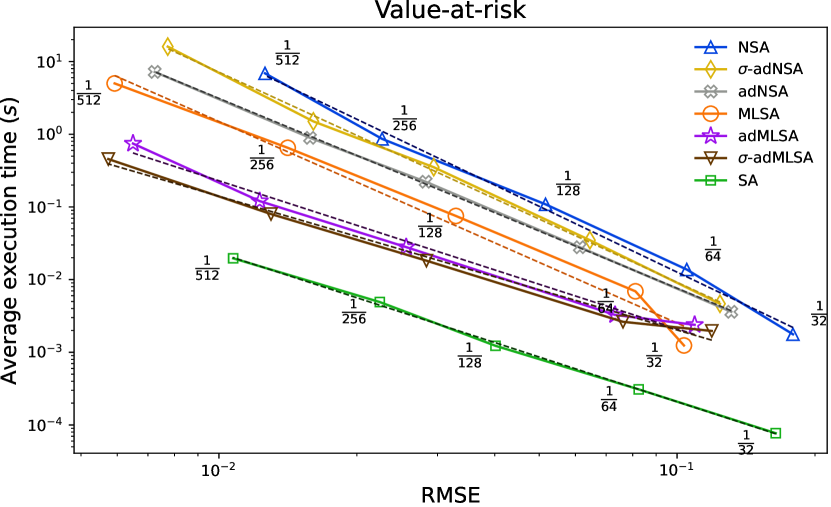
Figure 5.1: Performance comparison of the different SA schemes.

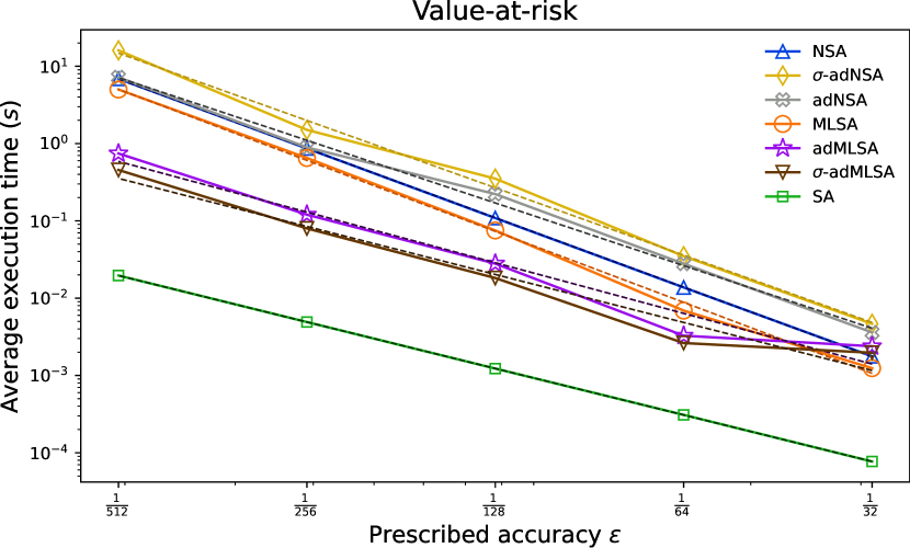
Figure 5.2: Complexity comparison of the different SA schemes.

SA scheme     NSA $\sigma$-adNSA adNSA MLSA adMLSA $\sigma$-adMLSA SA RMSE     $-3.01$ $-2.89$ $-2.61$ $-2.77$ $-2.04$ $-1.84$ $-2.05$ Accuracy $\varepsilon$     $-2.98$ $-2.89$ $-2.69$ $-3.05$ $-2.18$ $-2.06$ $-2.00$

Table 5.2: Reported slopes in Figures 5.1 and 5.2.

[13, Section 4.3] already provides a thorough discussion on (SA), (NSA) and (MLSA). We retain here that (MLSA) scores a partial gain on the performance gap between (SA) and (NSA).

The novelties here are the adaptive schemes. On Figure 5.1, (adNSA) and $\sigma$-(adNSA) achieve comparable performances, outperforming (NSA) by a margin that seems to widen for smaller accuracies. (adNSA) seems to be slightly outperforming $\sigma$-(adNSA), which can be attributed to the overhead computation performed by $\sigma$-(adNSA) to recompute the confidence constant $C_{a}$. (adMLSA) and $\sigma$-(adMLSA) show to be significantly outperforming (MLSA): for a target RMSE of order $10^{-2}$, (adMLSA) and $\sigma$-(adMLSA) run on average in $0.2\mathrm{s}$ while (MLSA) runs in $2\mathrm{s}$, achieving a $10$ fold speed-up over their non-adaptive counterpart. $\sigma$-(adMLSA) seems to slightly outperform (adMLSA), which can be explained by the precision brought by the recomputation of the standard deviation $\sigma$, in spite of the entailed overhead computational time. However, this overperformance remains slim, recalling that the calibrated confidence constant $C_{a}$ for (adMLSA) needs not be readjusted on the whole accuracy range once it has been optimized on a couple of accuracies, thus eliminating any additional upstream fine-tuning.

Eventually, an examination of the fitted slopes highlights that (adNSA) and $\sigma$-(adNSA) achieve the theoretical complexity exponents predicted by Proposition 3.5. It also demonstrates that (adMLSA) and $\sigma$-(adMLSA) achieve the quadratic complexity anticipated by Theorem 4.5(i) for $p_{\star}$ large. The performances of these schemes match that of (SA) that assumes the exact simulatability of the true loss $X_{0}$.

5.2 Interest Rate Swap

The following setting is recapitulated from [13, Section 5].

We consider a swap, of strike $\bar{K}$, maturity $T$ and nominal $\bar{N}$, each leg being worth $1$ at inception, issued at par on some underlying interest (or FX) rate $(S_{t})_{0\leq t\leq T}$ following a Black-Scholes model with risk neutral drift $\bar{\kappa}$ and constant volatility $\bar{\sigma}$. At the coupon dates $0<T_{1}<\dots<T_{d}=T$, the swap remunerates the cash flows $\Delta T_{i}(S_{T_{i-1}}-\bar{K})$, where $\Delta T_{i}=T_{i}-T_{i-1}$, $T_{0}=0$. The risk-free rate is $\bar{r}$ and the risk neutral probability measure is $\mathbb{P}$.

For $t\in[0,T]$, let $i_{t}$ be the integer such that $t\in[T_{i_{t}-1},T_{i_{t}})$ if $t\in[0,T)$, and $+\infty$ otherwise. The fair value of the swap at time $t\in[0,T]$ is

$$P_{t}=\bar{N}\,\mathbb{E}\bigg{[}\sum_{i=i_{t}}^{d}\mathrm{e}^{-\bar{r}(T_{i}-t)}\Delta T_{i}(S_{T_{i-1}}-\bar{K})\bigg{|}S_{t}\bigg{]}.$$

The loss on a short position on the swap at a time horizon $\tau\in(0,T_{1})$ is

$$X_{0}=\mathrm{e}^{-\bar{r}\tau}P_{\tau}.$$

We are interested in computing the VaR $\xi^{0}_{\star}$ of this loss at some confidence level $\alpha\in(0,1)$.

Analytical and Simulation Formulas.

On the one hand,

$$X_{0}\stackrel{{\scriptstyle\mathcal{L}}}{{=}}\bar{N}AS_{0}\Big{(}\exp\Big{(}-\frac{\bar{\sigma}^{2}}{2}\tau+\bar{\sigma}\sqrt{\tau}U\Big{)}-1\Big{)},\quad\mbox{ where }\quad A\coloneqq\sum_{i=2}^{d}\mathrm{e}^{-\bar{r}T_{i}}\Delta_{i}\mathrm{e}^{\bar{\kappa}T_{i-1}}$$

and $U\sim\mathcal{N}(0,1)$. This allows simulating $X_{0}$ exactly, hence the availability of (SA) to approximate the VaR.

On the other hand, $X_{0}$ satisfies

$$X_{0}\stackrel{{\scriptstyle\mathcal{L}}}{{=}}\mathbb{E}[\varphi(Y,Z)|Y],$$ (5.3)

where $Y\in\mathbb{R}$ is independent of $Z=(Z_{1},\dots,Z_{d-1})\in\mathbb{R}^{d-1}$, with

$$Y \coloneqq\exp\Big{(}-\frac{\bar{\sigma}^{2}}{2}\tau+\bar{\sigma}\sqrt{\tau}U_{0}\Big{)},$$

$$Z_{1} \coloneqq\exp\Big{(}-\frac{\bar{\sigma}^{2}}{2}(T_{1}-\tau)+\bar{\sigma}\sqrt{T_{1}-\tau}U_{1}\Big{)},$$

$$Z_{i} \coloneqq\exp\Big{(}-\frac{\bar{\sigma}^{2}}{2}\Delta_{i}+\bar{\sigma}\sqrt{\Delta_{i}}U_{i}\Big{)},\quad 2\leq i\leq d-1,$$

$$\varphi(y,z) \coloneqq\bar{N}S_{0}\sum_{i=2}^{d}\mathrm{e}^{-\bar{r}T_{i}}\Delta_{i}\mathrm{e}^{\bar{\kappa}T_{i-1}}\bigg{(}y\prod_{j=1}^{i-1}z_{j}-1\bigg{)},\quad y\in\mathbb{R},z=(z_{1},\dots,z_{d-1})\in\mathbb{R}^{d-1},$$

and $(U_{i})_{0\leq i\leq d-1}\stackrel{{\scriptstyle\text{\rm\tiny iid}}}{{\sim}}\mathcal{N}(0,1)$. The nested Monte Carlo averaging (1.6) is thus available to approximate (5.3), hence the applicability of (NSA), (adNSA), $\sigma$-(adNSA), (MLSA), (adMLSA) and $\sigma$-(adMLSA) to approximate the VaR.

Finally, the VaR $\xi^{0}_{\star}$ at level $\alpha$ is available analytically:

$$\xi^{0}_{\star}=\bar{N}AS_{0}\Big{(}\exp\Big{(}F^{-1}(\alpha)\bar{\sigma}\sqrt{\tau}-\frac{\bar{\sigma}^{2}}{2}\tau\Big{)}-1\Big{)},$$ (5.4)

where $F$ is the standard Gaussian cdf. The output of this formula will serve as a benchmark for the outcomes of the aforementioned algorithms.

Numerical Results.

For the case study, we set $S_{0}=1\%$, $\bar{r}=2\%$, $\bar{\kappa}=12\%$, $\bar{\sigma}=20\%$, $T=1\,\mathrm{year}$, $\Delta T_{i}=3\,\mathrm{months}$, $\tau=7\,\mathrm{days}$ and $\alpha=85\%$. We use the $30/360$ day count fraction convention. (5.4) yields $\xi^{0}_{\star}\approx 219.64$.

We run all algorithms at their theoretical optimums, with $\beta=1$ and the corresponding optimal iterations amounts. The learning rate $\gamma_{n}=100/n$ is employed for (SA) and $\gamma_{n}=50/n$ for (NSA), (adNSA) and $\sigma$-(adNSA). For (adNSA), $\sigma$-(adNSA), (MLSA), (adMLSA) and $\sigma$-(adMLSA), we adopt the framework (3.2) with the exponent $p_{\star}=8$, the geometric step $M=2$ and the exponent $\delta=0.95$ for $u_{n}$. As suggested in Section 4.3, we set $\theta=\frac{p_{\star}/2-1}{p_{\star}/2+1}$ and $r=1+\frac{1}{\theta}$. For every prescribed accuracy $\varepsilon\in\{\frac{1}{32},\frac{1}{64},\frac{1}{128},\frac{1}{256},\frac{1}{512}\}$, we tune $h_{0}$ (governing the number of levels $L$ for (MLSA), $\ell_{\mathrm{ad}}$ for (adNSA) and $\sigma$-(adNSA), and $L_{\mathrm{ad}}$ for (adMLSA) and $\sigma$-(adMLSA)) and the learning rate $(\gamma_{n})_{n\geq 1}$ for (MLSA), (adMLSA) and $\sigma$-(adMLSA) on suitable grids. Table 5.3 lists these parametrizations by prescribed accuracy. The iterations amounts scaling factor $C$ and adaptive refinement confidence constant $C_{a}$ are tuned on grids. We retain $C=80$ for (adMLSA) and $\sigma$-(adMLSA), $C_{a}=100$ for (adMLSA), $C=2$ for (adNSA) and $\sigma$-(adNSA) and $C_{a}=300$ for (adNSA). We eventually set the critical value $C_{p}=3$ for $\sigma$-(adNSA) and $\sigma$-(adMLSA).

$\varepsilon$ $h_{0}$ $\ell_{\mathrm{ad}}$ $\frac{1}{32}$ $\frac{1}{8}$ $2$ $\frac{1}{64}$ $\frac{1}{16}$ $2$ $\frac{1}{128}$ $\frac{1}{16}$ $2$ $\frac{1}{256}$ $\frac{1}{16}$ $3$ $\frac{1}{512}$ $\frac{1}{16}$ $4$ $\varepsilon$ $h_{0}$ $L$ $\gamma_{n}$ $\frac{1}{32}$ $\frac{1}{8}$ $2$ $\frac{6}{10+n}$ $\frac{1}{64}$ $\frac{1}{16}$ $2$ $\frac{20}{500+n}$ $\frac{1}{128}$ $\frac{1}{16}$ $3$ $\frac{21}{10^{3}+n}$ $\frac{1}{256}$ $\frac{1}{16}$ $4$ $\frac{20}{2\times 10^{3}+n}$ $\frac{1}{512}$ $\frac{1}{16}$ $5$ $\frac{21}{3\times 10^{3}+n}$ $\varepsilon$ $h_{0}$ $L_{\mathrm{ad}}$ $\gamma_{n}$ $\frac{1}{32}$ $\frac{1}{8}$ $2$ $\frac{6}{10+n}$ $\frac{1}{64}$ $\frac{1}{16}$ $2$ $\frac{20}{500+n}$ $\frac{1}{128}$ $\frac{1}{16}$ $2$ $\frac{21}{10^{3}+n}$ $\frac{1}{256}$ $\frac{1}{16}$ $3$ $\frac{20}{2\times 10^{3}+n}$ $\frac{1}{512}$ $\frac{1}{16}$ $4$ $\frac{21}{3\times 10^{3}+n}$

Table 5.3: Parametrizations of (adNSA) and $\sigma$-(adNSA) (left), (MLSA) (center) and (adMLSA) and $\sigma$-(adMLSA) (right), by prescribed accuracy.

The joint evolution of the RMSE and average execution time over $200$ runs of each SA scheme, for an accuracy $\varepsilon$ looping through $\{\frac{1}{32},\frac{1}{64},\frac{1}{128},\frac{1}{256},\frac{1}{512}\}$, are plotted on a logarithmic scale on Figure 5.3. Figure 5.4 showcases the average execution times against the prescribed accuracies. Table 5.4 reports the regressed slopes on these curves as depicted in dashed lines on Figures 5.3 and 5.4.

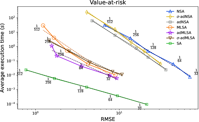
Figure 5.3: Performance comparison of the different SA schemes.

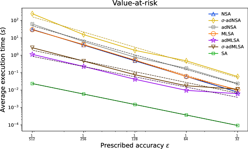
Figure 5.4: Complexity comparison of the different SA schemes.

SA scheme     NSA $\sigma$-adNSA adNSA MLSA adMLSA $\sigma$-adMLSA SA RMSE     $-3.52$ $-4.10$ $-3.86$ $-3.93$ $-2.60$ $-2.75$ $-1.66$ Accuracy $\varepsilon$     $-3.00$ $-2.90$ $-2.78$ $-2.90$ $-1.96$ $-2.05$ $-2.00$

Table 5.4: Reported slopes in Figures 5.3 and 5.4.

We refer to [13, Section 5.3] for extended comments on (SA), (NSA) and (MLSA).

Similar comments to the previous case study are applicable here. For smaller accuracies, (adNSA) and $\sigma$-(adNSA) score a speed-up with respect to (NSA) as do (adMLSA) and $\sigma$-(adMLSA) with respect to (MLSA). The performance margins between (adNSA) and $\sigma$-(adNSA) on the one hand and (adMLSA) and $\sigma$-(adMLSA) on the other hand are rather slim. (adNSA) and (adMLSA) remain preferable as they do not require recomputing $C_{a}$ once it has been fine-tuned on a couple of prescribed accuracies.

Although further fine-tuning may be required, the fitted slopes already indicate that the adaptive multilevel schemes are approaching the desired quadratic complexity.

Conclusion

For a prescribed accuracy $\varepsilon\in(0,1)$, the canonical $\varepsilon^{-2}$ multilevel complexity order is retrieved, up to a logarithmic factor, for an MLSA scheme with a Heaviside-type update function. This is made possible by adopting an adaptive refinement strategy on the innovations driving the multilevel algorithm’s inner nested schemes. Our strategy allows to fulfill the closure of the performance gap that resides between nested MLSA and unbiased Robbins-Monro schemes for Heaviside-type update functions. The performance gain achieved by adaptive MLSA on its regular counterpart is significant in practice, attaining a ten fold speed-up in certain cases and expected to increase exponentially with smaller prescribed accuracies.

A potential future line of research could involve applying a Polyak-Ruppert averaging [14] to (adMLSA) to promote greater numerical stability. We could also explore extending our findings on adaptive refinement to include triply nested X-value adjustment estimations [25].

Appendix A Auxiliary Results

The proof of the following result is included in the preliminary steps of [13, Proposition 3.2] and is therefore omitted.

Lemma A.1.

1. Assume that there exists $p\geq 1$ such that $\mathbb{E}[|\varphi(Y,Z)-\mathbb{E}[\varphi(Y,Z)|Y]|^{p}]<\infty$. Then, for any $h,h^{\prime}\in\overline{\mathcal{H}}$,

   $$\mathbb{E}[|X_{h}-X_{h^{\prime}}|^{p}]\leq C|h-h^{\prime}|^{\frac{p}{2}}.$$

2. Assume that there exists $C_{g}>0$ such that $\mathbb{E}\big{[}\exp\big{(}u\big{(}\varphi(Y,Z)-\mathbb{E}[\varphi(Y,Z)|Y]\big{)}\big{)}\big{|}Y\big{]}\leq\mathrm{e}^{C_{g}u^{2}}$ $\mathbb{P}\text{\rm-as}$ for all $u\in\mathbb{R}$. Then, for any $h,h^{\prime}\in\overline{\mathcal{H}}$ and any $u\in\mathbb{R}$,

   $$\mathbb{E}\big{[}\exp\big{(}u(X_{h}-X_{h^{\prime}})\big{)}\big{|}Y\big{]}\leq\exp\big{(}C_{g}u^{2}|h-h^{\prime}|\big{)}\quad\mbox{ holds $\mathbb{P}\text{\rm-as}$.}$$

Similarly to [13], we define, for $h\in\overline{\mathcal{H}}$, $\mu\geq 0$ and a positive integer $q$, the Lyapunov function $\mathcal{L}^{\mu}_{h,q}\colon\mathbb{R}\to\mathbb{R}_{+}$ by

$$\mathcal{L}^{\mu}_{h,q}(\xi)=\big{(}V_{h}(\xi)-V_{h}(\xi^{h}_{\star})\big{)}^{q}\exp\big{(}\mu\big{(}V_{h}(\xi)-V_{h}(\xi^{h}_{\star})\big{)}\big{)},\quad\xi\in\mathbb{R}.$$ (A.1)

The following lemma states some important properties of $\mathcal{L}^{\mu}_{h,q}$.

Lemma A.2 ([13, Lemma 3.2]).

Denote $k_{\alpha}=1\vee\frac{\alpha}{1-\alpha}$, $\mu_{h,q}=q^{2}\|V_{h}^{\prime\prime}\|_{\infty}$ and $\bar{\mathcal{L}}_{h,q}=\mathcal{L}^{\mu_{h,q}}_{h,q}$, $h\in\overline{\mathcal{H}}$, $q\in\mathbb{N}_{0}$. Under Assumption 1.1, for any $h\in\overline{\mathcal{H}}$, $\mu\geq 0$ and $q\geq 1$,

1. $\mathcal{L}^{\mu}_{h,q}$ is twice continuously differentiable on $\mathbb{R}$ and

   $$(\mathcal{L}^{\mu}_{h,q})^{\prime}(\xi)=qV_{h}^{\prime}(\xi)\mathcal{L}^{\mu}_{h,q-1}(\xi)+\mu V_{h}^{\prime}(\xi)\mathcal{L}^{\mu}_{h,q}(\xi),\quad\xi\in\mathbb{R}.$$ (A.2)

2. for any $\xi\in\mathbb{R}$,

   $$\bar{\mathcal{L}}_{h,q}(\xi)\leq k_{\alpha}^{q}\,|\xi-\xi^{h}_{\star}|^{q}\exp\Big{(}\frac{q^{2}}{1-\alpha}k_{\alpha}\sup_{h\in\overline{\mathcal{H}}}\|f_{X_{h}}\|_{\infty}|\xi-\xi^{h}_{\star}|\Big{)}.$$

3. for any $\xi\in\mathbb{R}$,

   $$V_{h}^{\prime}(\xi)(\mathcal{L}^{\mu}_{h,q})^{\prime}(\xi)\geq\lambda^{\mu}_{h,q}\mathcal{L}^{\mu}_{h,q}(\xi),\quad\mbox{ where }\quad\lambda^{\mu}_{h,q}\coloneqq\frac{3}{8}qV_{h}^{\prime\prime}(\xi^{h}_{\star})\wedge\mu\frac{V_{h}^{\prime\prime}(\xi^{h}_{\star})^{4}}{4[V_{h}^{\prime\prime}]_{\text{\rm Lip}}^{2}}.$$

   Let $\bar{\lambda}_{h,q}\coloneqq\lambda^{\mu_{h,q}}_{h,q}$. Then $\inf_{h\in\overline{\mathcal{H}}}{\bar{\lambda}_{h,q}}>0$.

4. for any $\xi\in\mathbb{R}$,

   $$|(\mathcal{L}^{\mu}_{h,q})^{\prime\prime}(\xi)|\leq\eta^{\mu}_{h,q}\big{(}\mathcal{L}^{\mu}_{h,q}(\xi)+\mathcal{L}^{\mu}_{h,q-1}(\xi)\big{)},$$

   where

   $$\eta^{\mu}_{h,q}\coloneqq(q\vee\mu)\|V_{h}^{\prime\prime}\|_{\infty}+k_{\alpha}^{2}\mu(\mu\vee 2)+q(2\mu\vee(q-1))\Big{(}\frac{3k_{\alpha}^{2}[V_{h}^{\prime\prime}]_{\text{\rm Lip}}^{2}}{V_{h}^{\prime\prime}(\xi^{h}_{\star})^{3}}\vee\frac{3\|V_{h}^{\prime\prime}\|_{\infty}^{2}}{V_{h}^{\prime\prime}(\xi^{h}_{\star})}\Big{)}.$$

   Besides, introducing $\bar{\eta}_{h,q}\coloneqq\eta^{\mu_{h,q}}_{h,q}$, one has $|\bar{\lambda}_{h,q}|^{2}\leq\bar{\eta}_{h,q}$ and $\sup_{h\in\overline{\mathcal{H}}}{\bar{\eta}_{h,q}}<\infty$.

5. for any $\xi\in\mathbb{R}$,

   $$(\xi-\xi^{h}_{\star})^{2q}\leq\kappa_{h,q}\big{(}\mathcal{L}^{\mu}_{h,q}(\xi)+\mathcal{L}^{\mu}_{h,2q}(\xi)\big{)},\quad\mbox{ where }\quad\kappa_{h,q}\coloneqq\frac{3^{q}}{V_{h}^{\prime\prime}(\xi^{h}_{\star})^{q}}\vee\frac{3^{2q}[V_{h}^{\prime\prime}]_{\text{\rm Lip}}^{2q}}{V_{h}^{\prime\prime}(\xi^{h}_{\star})^{4q}}.$$

   Moreover, $\sup_{h\in\overline{\mathcal{H}}}{\kappa_{h,q}}<\infty$.

Appendix B Proofs of the Auxiliary Convergence Results

Throughout, $C<\infty$ denotes a positive constant that may change from line to line but is independent of $n$ and $\ell$.

Proof of Lemma 2.1.

The proof is similar to [13, Proposition 4.2(ii)]. We have

$$\mathbb{E}\big{[}\big{|}\mathds{1}_{X_{h^{\prime}}>\xi} -\mathds{1}_{X_{h}>\xi}\big{|}\big{]}$$

$$=\mathbb{P}(X_{h^{\prime}}\leq\xi<X_{h})+\mathbb{P}(X_{h}\leq\xi<X_{h^{\prime}})$$

$$=\mathbb{P}(X_{h}+{(h^{\prime})}^{\frac{1}{2}}G_{h}^{h^{\prime}}\leq\xi<X_{h})+\mathbb{P}(X_{h}\leq\xi<X_{h}+{(h^{\prime})}^{\frac{1}{2}}G_{h}^{h^{\prime}})$$

$$=\mathbb{P}(X_{h}-{(h^{\prime})}^{\frac{1}{2}}(G_{h}^{h^{\prime}})^{-}\leq\xi<X_{h})+\mathbb{P}(X_{h}\leq\xi<X_{h}+{(h^{\prime})}^{\frac{1}{2}}(G_{h}^{h^{\prime}})^{+})$$

$$=\mathbb{E}\big{[}F_{X_{h}|G_{h}^{h^{\prime}}}(\xi+(h^{\prime})^{\frac{1}{2}}(G_{h}^{h^{\prime}})^{-})-F_{X_{h}|G_{h}^{h^{\prime}}}(\xi)\big{]}$$

$$\qquad+\mathbb{E}\big{[}F_{X_{h}|G_{h}^{h^{\prime}}}(\xi)-F_{X_{h}|G_{h}^{h^{\prime}}}(\xi-(h^{\prime})^{\frac{1}{2}}(G_{h}^{h^{\prime}})^{+})\big{]}$$

$$=\mathbb{E}\big{[}F_{X_{h}|G_{h}^{h^{\prime}}}(\xi+(h^{\prime})^{\frac{1}{2}}(G_{h}^{h^{\prime}})^{-})-F_{X_{h}|G_{h}^{h^{\prime}}}(\xi-(h^{\prime})^{\frac{1}{2}}(G_{h}^{h^{\prime}})^{+})\big{]}$$

$$\leq\big{(}\!\sup_{0\leq h_{1}<h_{2}\in\overline{\mathcal{H}}}{\mathbb{E}[K_{h_{1}}^{h_{2}}|G_{h_{1}}^{h_{2}}|]}\big{)}(h^{\prime})^{\frac{1}{2}}.$$

∎

Proof of Lemma 3.1.

By (2.8) and the law of total probability,

$$\mathbb{P}(X_{h_{\ell+\eta^{n}_{\ell}(\xi)}}\leq\xi) -F_{X_{h_{\ell+\lceil\theta\ell\rceil}}}(\xi)$$ (B.1)

$$=\sum_{k=0}^{\lceil\theta\ell\rceil}\mathbb{P}(X_{h_{\ell+k}}\leq\xi,\eta_{\ell}^{n}(\xi)=k)-\mathbb{P}(X_{h_{\ell+\lceil\theta\ell\rceil}}\leq\xi,\eta_{\ell}^{n}(\xi)=k)$$

$$=\sum_{k=0}^{\lceil\theta\ell\rceil-1}\mathbb{E}\big{[}\big{(}\mathds{1}_{X_{h_{\ell+k}}\leq\xi}-\mathds{1}_{X_{h_{\ell+\lceil\theta\ell\rceil}}\leq\xi}\big{)}\mathds{1}_{\eta_{\ell}^{n}(\xi)=k}\big{]}.$$

(i) a. For $k\in[\![0,\lceil\theta\ell\rceil-1]\!]$, given that

$$\{X_{h_{\ell+k}}\leq\xi<X_{h_{\ell+\lceil\theta\ell\rceil}}\}\sqcup\{X_{h_{\ell+\lceil\theta\ell\rceil}}\leq\xi<X_{h_{\ell+k}}\}\subset\{|X_{h_{\ell+k}}-X_{h_{\ell+\lceil\theta\ell\rceil}}|\geq|X_{h_{\ell+k}}-\xi|\}$$ (B.2)

and that, by (2.8) under the condition (1.16),

$$\{\eta^{n}_{\ell}(\xi)=k\}\subset\big{\{}|X_{h_{\ell+k}}-\xi|\geq C_{a}u_{n}^{-\frac{1}{p_{\star}}}h_{\theta\ell(r-1)+k}^{\frac{1}{r}}\big{\}},$$ (B.3)

by Markov’s inequality and Lemma A.1(i),

$$\big{|}\mathbb{E}\big{[}\big{(}\mathds{1}_{X_{h_{\ell+k}}\leq\xi} -\mathds{1}_{X_{h_{\ell+\lceil\theta\ell\rceil}}\leq\xi}\big{)}\mathds{1}_{\eta^{n}_{\ell}(\xi)=k}\big{]}\big{|}$$

$$\leq\mathbb{E}\Big{[}\Big{(}\mathds{1}_{X_{h_{\ell+k}}\leq\xi<X_{h_{\ell+\lceil\theta\ell\rceil}}}+\mathds{1}_{X_{h_{\ell+\lceil\theta\ell\rceil}}\leq\xi<X_{h_{\ell+k}}}\Big{)}\mathds{1}_{\big{\{}|X_{h_{\ell+k}}-\xi|\geq C_{a}u_{n}^{-\frac{1}{p_{\star}}}h_{\theta\ell(r-1)+k}^{\frac{1}{r}}\big{\}}}\Big{]}$$

$$\leq\mathbb{P}\big{(}|X_{h_{\ell+k}}-X_{h_{\ell+\lceil\theta\ell\rceil}}|\geq|X_{h_{\ell+k}}-\xi|,|X_{h_{\ell+k}}-\xi|\geq C_{a}u_{n}^{-\frac{1}{p_{\star}}}h_{\theta\ell(r-1)+k}^{\frac{1}{r}}\big{)}$$

$$\leq C_{a}^{-p_{\star}}u_{n}h_{\theta\ell(r-1)+k}^{-\frac{p_{\star}}{r}}\,\mathbb{E}[|X_{h_{\ell+k}}-X_{h_{\ell+\lceil\theta\ell\rceil}}|^{p_{\star}}]$$

$$\leq Cu_{n}h_{\theta\ell(r-1)+k}^{-\frac{p_{\star}}{r}}h_{\ell+k}^{\frac{p_{\star}}{2}}.$$

Using the previous inequality, (B.1) and the condition (3.2) on $r$ then on $\theta$,

$$\big{|}\mathbb{P}(X_{h_{\ell+\eta^{n}_{\ell}(\xi)}}\leq\xi) -F_{X_{h_{\ell+\lceil\theta\ell\rceil}}}(\xi)\big{|}$$ (B.4)

$$\leq Cu_{n}h_{\theta\ell(r-1)}^{-\frac{p_{\star}}{r}}h_{\ell}^{\frac{p_{\star}}{2}}\sum_{k=0}^{\lceil\theta\ell\rceil-1}h_{k}^{(\frac{1}{2}-\frac{1}{r})p_{\star}}$$

$$\leq Cu_{n}h_{-\theta\ell p_{\star}(1-\frac{1}{r})+\frac{p_{\star}\ell}{2}+\theta\ell p_{\star}(\frac{1}{2}-\frac{1}{r})}$$

$$\leq Cu_{n}h_{\ell}^{1+\theta}.$$

(i) b. Let $k\in[\![0,\lceil\theta\ell\rceil-1]\!]$ and $\lambda>0$. By (B.2), (B.3), the definition (2.8) in the case of (1.17), Markov’s exponential inequality and Lemma A.1(i),

$$\big{|}\mathbb{E}\big{[}\big{(}\mathds{1}_{X_{h_{\ell+k}}\leq\xi} -\mathds{1}_{X_{h_{\ell+\lceil\theta\ell\rceil}}\leq\xi}\big{)}\mathds{1}_{\eta^{n}_{\ell}(\xi)=k}\big{]}\big{|}$$

$$\leq\mathbb{P}\big{(}|X_{h_{\ell+k}}-X_{h_{\ell+\lceil\theta\ell\rceil}}|\geq|X_{h_{\ell+k}}-\xi|,|X_{h_{\ell+k}}-\xi\big{|}\geq C_{a}h^{\frac{1}{r}}_{\theta\ell(r-1)+k}\big{(}\ln{\gamma_{n}^{-\frac{1}{2}}h^{-\frac{1}{2}(1+\theta)}_{\ell+k}}\big{)}^{\frac{1}{2}}\big{)}$$

$$\leq\exp\big{(}-C_{a}\lambda h^{\frac{1}{r}}_{\theta\ell(r-1)+k}\big{(}\ln{\gamma_{n}^{-\frac{1}{2}}h^{-\frac{1}{2}(1+\theta)}_{\ell+k}}\big{)}^{\frac{1}{2}}\big{)}\mathbb{E}[\exp(\lambda|X_{h_{\ell+k}}-X_{h_{\ell+\lceil\theta\ell\rceil}}|)]$$

$$\leq 2\exp\big{(}-C_{a}\lambda h^{\frac{1}{r}}_{\theta\ell(r-1)+k}\big{(}\ln{\gamma_{n}^{-\frac{1}{2}}h^{-\frac{1}{2}(1+\theta)}_{\ell+k}}\big{)}^{\frac{1}{2}}+C_{g}\lambda^{2}h_{\ell+k}\big{)}.$$

Minimizing the above upper bound with respect to $\lambda$ yields

$$\big{|}\mathbb{E}\big{[}\big{(}\mathds{1}_{X_{h_{\ell+k}}\leq\xi}-\mathds{1}_{X_{h_{\ell+\lceil\theta\ell\rceil}}\leq\xi}\big{)}\mathds{1}_{\eta_{\ell}^{n}(\xi)=k}\big{]}\big{|}\leq 2\exp\bigg{(}-\frac{C_{a}^{2}h^{\frac{2}{r}}_{\theta\ell(r-1)+k}\ln{\gamma_{n}^{-\frac{1}{2}}h^{-\frac{1}{2}(1+\theta)}_{\ell+k}}}{4C_{g}h_{\ell+k}}\bigg{)}.$$

In view of the condition (3.3) on $h_{0}$, $r$ and $\theta$, one gets

$$\big{|}\mathbb{E}\big{[}\big{(}\mathds{1}_{X_{h_{\ell+k}}\leq\xi}-\mathds{1}_{X_{h_{\ell+\lceil\theta\ell\rceil}}\leq\xi}\big{)}\mathds{1}_{\eta_{\ell}^{n}(\xi)=k}\big{]}\big{|}\leq 2\big{(}\gamma_{n}h_{\ell+k}^{1+\theta}\big{)}^{\frac{C_{a}^{2}h_{0}^{2/r-1}}{8C_{g}}M^{-2\theta\ell(1-\frac{1}{r})+\ell}}\leq 2\gamma_{n}h_{\ell+k}^{1+\theta}.$$

Therefore, recalling (B.1),

$$\big{|}\mathbb{P}(X_{h_{\ell+\eta^{n}_{\ell}(\xi)}}\leq\xi)-F_{X_{h_{\ell+\lceil\theta\ell\rceil}}}(\xi)\big{|}\leq C\gamma_{n}h_{\ell}^{1+\theta}.$$ (B.5)

(ii) For $k\in[\![0,\lceil\theta\ell\rceil-1]\!]$, via the definition (2.8) in the case of (2.7), Markov’s exponential inequality and the condition (3.4) on $h_{0}$, $r$ and $\theta$,

$$\big{|}\mathbb{E}\big{[}\big{(}\mathds{1}_{X_{h_{\ell+k}}>\xi} -\mathds{1}_{X_{h_{\ell+\lceil\theta\ell\rceil}}>\xi}\big{)}\mathds{1}_{\eta^{n}_{\ell}(\xi)=k}\big{]}\big{|}$$

$$\leq\mathbb{P}\big{(}|X_{h_{\ell+k}}-X_{h_{\ell+\lceil\theta\ell\rceil}}|\geq|X_{h_{\ell+k}}-\xi|,|X_{h_{\ell+k}}-\xi\big{|}\geq C_{a}h^{\frac{1}{r}}_{\theta\ell(r-1)+k}\big{(}\ln{\gamma_{n}^{-\frac{1}{2}}h_{\ell+k}^{-\frac{1}{2}(1+\theta)}}\big{)}^{\frac{1}{2}}\big{)}$$

$$\leq\mathbb{P}\big{(}\big{|}G_{h_{\ell+\lceil\theta\ell\rceil}}^{h_{\ell+k}}\big{|}\geq C_{a}h^{\frac{1}{r}}_{\theta\ell(r-1)+k}h_{\ell+k}^{-\frac{1}{2}}\big{(}\ln{\gamma_{n}^{-\frac{1}{2}}h_{\ell+k}^{-\frac{1+\theta}{2}}}\big{)}^{\frac{1}{2}}\big{)}$$

$$\leq\exp{\big{(}-\upsilon_{0}C_{a}^{2}h_{\theta\ell(r-1)+k}^{\frac{2}{r}}h_{\ell+k}^{-1}\ln{\gamma_{n}^{-\frac{1}{2}}h_{\ell+k}^{-\frac{1+\theta}{2}}}\big{)}}\mathbb{E}\big{[}\exp\big{(}\upsilon_{0}\big{|}G_{h_{\ell+\lceil\theta\ell\rceil}}^{h_{\ell+k}}\big{|}^{2}\big{)}\big{]}$$

$$\leq\big{(}\!\sup_{0\leq h<h^{\prime}\in\overline{\mathcal{H}}}\mathbb{E}\big{[}\exp(\upsilon_{0}|G_{h}^{h^{\prime}}|^{2})\big{]}\big{)}\big{(}h_{\ell+k}^{1+\theta}\gamma_{n}\big{)}^{\frac{1}{2}\upsilon_{0}C_{a}^{2}h_{0}^{\frac{2}{r}-1}M^{-2\theta\ell(1-\frac{1}{r})+\ell}}$$

$$\leq C\gamma_{n}h_{\ell+k}^{1+\theta}.$$

Thus, by (B.1),

$$\big{|}\mathbb{P}(X_{h_{\ell+\eta^{n}_{\ell}(\xi)}}\leq\xi)-F_{X_{h_{\ell+\lceil\theta\ell\rceil}}}(\xi)\big{|}\leq C\gamma_{n}h_{\ell}^{1+\theta}.$$ (B.6)

Eventually, we decompose

$$\mathbb{P}(X_{h_{\ell+\eta_{\ell}(\xi)}}\leq\xi)-F_{X_{0}}(\xi)=\underbrace{\big{(}\mathbb{P}(X_{h_{\ell+\eta_{\ell}^{n}(\xi)}}\leq\xi)-F_{X_{h_{\ell+\lceil\theta\ell\rceil}}}(\xi)\big{)}}_{\eqqcolon A_{\ell}^{n}}+\underbrace{\big{(}F_{X_{h_{\ell+\lceil\theta\ell\rceil}}}(\xi)-F_{X_{0}}(\xi)\big{)}}_{\eqqcolon B_{\ell}}.$$

By (B.4)–(B.6) and Assumption 1.1(i),

$$|A_{\ell}^{n}|\leq C\gamma_{1}h_{\ell}^{1+\theta},\quad B_{\ell}=-\frac{v(\xi^{0}_{\star})}{f_{X_{0}}(\xi^{0}_{\star})}h_{\ell+\lceil\theta\ell\rceil}+\mathrm{o}(h_{\ell+\lceil\theta\ell\rceil}),$$

hence the final result.

∎

Proof of Proposition 3.2.

In this proof, we omit the superscript $\mu$ from the Lyapunov function $\mathcal{L}^{\mu}_{h,q}$ and denote instead $\mathcal{L}_{h,q}$. For any $\ell\geq 0$, let $(\widetilde{\mathcal{F}}^{h_{\ell}}_{n})_{n\geq 0}$ be the filtration defined by $\widetilde{\mathcal{F}}^{h_{\ell}}_{0}=\sigma(\widetilde{\xi}^{h_{\ell}}_{0})$ and $\widetilde{\mathcal{F}}^{h_{\ell}}_{n}=\sigma(\widetilde{\xi}^{h_{\ell}}_{0},X_{h_{\ell+\lceil\theta\ell\rceil}}^{(1)},\dots,X_{h_{\ell+\lceil\theta\ell\rceil}}^{(n)})$, $n\geq 1$.

For $\ell\geq 1$ and $n\geq 1$, define

$$\mathpzc{v}_{\ell}^{n}(\xi)\coloneqq\mathbb{E}\big{[}H\big{(}\xi,X_{h_{\ell+\eta_{\ell}^{n}(\xi)}}\big{)}\big{]}=1-\frac{1}{1-\alpha}\mathbb{P}\big{(}X_{h_{\ell+\eta_{\ell}^{n}(\xi)}}\geq\xi\big{)},\quad\xi\in\mathbb{R}.$$ (B.7)

The dynamics (adNSA) rewrite

$$\widetilde{\xi}^{h_{\ell}}_{n+1}=\widetilde{\xi}^{h_{\ell}}_{n}-\gamma_{n+1}V_{h_{\ell+\lceil\theta\ell\rceil}}^{\prime}(\widetilde{\xi}^{h_{\ell}}_{n})-\gamma_{n+1}r^{h_{\ell}}_{n+1}-\gamma_{n+1}e^{h_{\ell}}_{n+1},$$ (B.8)

where

$$r^{h_{\ell}}_{n+1} \coloneqq\mathpzc{v}_{\ell}^{n+1}(\widetilde{\xi}^{h_{\ell}}_{n})-V_{h_{\ell+\lceil\theta\ell\rceil}}^{\prime}(\widetilde{\xi}^{h_{\ell}}_{n}),$$ (B.9)

$$e^{h_{\ell}}_{n+1} \coloneqq H(\widetilde{\xi}_{n}^{h_{\ell}},\widetilde{X}^{(n+1)}_{h_{\ell}})-\mathpzc{v}_{\ell}^{n+1}(\widetilde{\xi}^{h_{\ell}}_{n}).$$ (B.10)

By Lemma 3.1,

$$|r_{n+1}^{h_{\ell}}|=\frac{1}{1-\alpha}\big{|}\mathbb{P}(X_{h_{\ell+\eta_{\ell}^{n+1}(\xi)}}\leq\xi)_{|\widetilde{\xi}^{h_{\ell}}_{n}}-\mathbb{P}(X_{h_{\ell+\lceil\theta\ell\rceil}}\leq\xi)_{|\widetilde{\xi}^{h_{\ell}}_{n}}\big{|}\leq Ch_{\ell+\lceil\theta\ell\rceil}\widetilde{u}_{n+1},$$ (B.11)

where

$$\widetilde{u}_{n+1}\coloneqq\begin{cases}u_{n+1}&\text{if\leavevmode\nobreak\ \eqref{assumption:finite:Lp:moment} holds,}\\ \gamma_{n+1}&\text{if\leavevmode\nobreak\ \eqref{assumption:conditional:gaussian:concentration} or\leavevmode\nobreak\ \eqref{assump:unif:lipschitz:integrability:conditional:cdf:bis} holds.}\end{cases}$$ (B.12)

Let $q\geq 1$. In the spirit of [13, Theorem 3.3], we test the Lyapunov $\mathcal{L}_{h_{\ell+\lceil\theta\ell\rceil},q}$ along the dynamics (B.8). Using a second order Taylor expansion,

$$\mathcal{L}_{h_{\ell+\lceil\theta\ell\rceil},q}(\widetilde{\xi}^{h_{\ell}}_{n+1}) =\mathcal{L}_{h_{\ell+\lceil\theta\ell\rceil},q}\big{(}\widetilde{\xi}^{h_{\ell}}_{n}-\gamma_{n+1}V_{h_{\ell+\lceil\theta\ell\rceil}}^{\prime}(\widetilde{\xi}^{h_{\ell}}_{n})-\gamma_{n+1}r^{h_{\ell}}_{n+1}-\gamma_{n+1}e^{h_{\ell}}_{n+1}\big{)}$$ (B.13)

$$=\mathcal{L}_{h_{\ell+\lceil\theta\ell\rceil},q}(\widetilde{\xi}^{h_{\ell}}_{n})-\gamma_{n+1}\mathcal{L}_{h_{\ell+\lceil\theta\ell\rceil},q}^{\prime}(\widetilde{\xi}^{h_{\ell}}_{n})(V_{h_{\ell+\lceil\theta\ell\rceil}}^{\prime}(\widetilde{\xi}^{h_{\ell}}_{n})+r_{n+1}^{h_{\ell}}+e^{h_{\ell}}_{n+1})$$

$$\quad+\gamma_{n+1}^{2}H(\widetilde{\xi}^{h_{\ell}}_{n},\widetilde{X}_{h_{\ell}}^{(n+1)})^{2}\int_{0}^{1}(1-t)\mathcal{L}_{h_{\ell+\lceil\theta\ell\rceil},q}^{\prime\prime}(t\widetilde{\xi}^{h_{\ell}}_{n+1}+(1-t)\widetilde{\xi}^{h_{\ell}}_{n})\,\mathrm{d}t.$$

It follows from Lemmas A.2(iii,iv), (A.2) and (B.11) that

$$\mathcal{L}_{h_{\ell+\lceil\theta\ell\rceil},q} (\widetilde{\xi}^{h_{\ell}}_{n+1})\leq\mathcal{L}_{h_{\ell+\lceil\theta\ell\rceil},q}(\widetilde{\xi}^{h_{\ell}}_{n})\big{(}1-\lambda^{\mu}_{h_{\ell+\lceil\theta\ell\rceil},q}\gamma_{n+1}+C\mu\|V_{h_{\ell+\lceil\theta\ell\rceil}}^{\prime}\|_{\infty}h_{\ell+\lceil\theta\ell\rceil}\gamma_{n+1}\widetilde{u}_{n+1}\big{)}$$ (B.14)

$$-\gamma_{n+1}\mathcal{L}_{h_{\ell+\lceil\theta\ell\rceil},q}^{\prime}(\widetilde{\xi}^{h_{\ell}}_{n})e^{h_{\ell}}_{n+1}+Cq\|V_{h_{\ell+\lceil\theta\ell\rceil}}^{\prime}\|_{\infty}h_{\ell+\lceil\theta\ell\rceil}\gamma_{n+1}\widetilde{u}_{n+1}\mathcal{L}_{h_{\ell+\lceil\theta\ell\rceil},q-1}(\widetilde{\xi}^{h_{\ell}}_{n})$$

$$+\eta^{\mu}_{h_{\ell+\lceil\theta\ell\rceil},q}\gamma_{n+1}^{2}H(\widetilde{\xi}^{h_{\ell}}_{n},\widetilde{X}_{h_{\ell}}^{(n+1)})^{2}$$

$$\quad\times\int_{0}^{1}(1-t)\big{(}\mathcal{L}_{h_{\ell+\lceil\theta\ell\rceil},q}(t\widetilde{\xi}^{h_{\ell}}_{n+1}+(1-t)\widetilde{\xi}^{h_{\ell}}_{n})+\mathcal{L}_{h_{\ell+\lceil\theta\ell\rceil},q-1}(t\widetilde{\xi}^{h_{\ell}}_{n+1}+(1-t)\widetilde{\xi}^{h_{\ell}}_{n})\big{)}\mathrm{d}t.$$

The mean value theorem guarantees that, for any $t\in[0,1]$, there exists $a^{h_{\ell}}_{n}(t)\in\mathbb{R}$ such that

$$V_{h_{\ell+\lceil\theta\ell\rceil}}(t\widetilde{\xi}^{h_{\ell}}_{n+1}+(1-t)\widetilde{\xi}^{h_{\ell}}_{n})=V_{h_{\ell+\lceil\theta\ell\rceil}}(\widetilde{\xi}^{h_{\ell}}_{n})+tV^{\prime}_{h_{\ell+\lceil\theta\ell\rceil}}(a^{h_{\ell}}_{n}(t))(\widetilde{\xi}^{h_{\ell}}_{n+1}-\widetilde{\xi}^{h_{\ell}}_{n}).$$ (B.15)

Besides, from (1.3),

$$|\widetilde{\xi}^{h_{\ell}}_{n+1}-\widetilde{\xi}^{h_{\ell}}_{n}|=\gamma_{n+1}|H(\widetilde{\xi}^{h_{\ell}}_{n},\widetilde{X}_{h_{\ell}}^{(n+1)})|\leq k_{\alpha}\gamma_{n+1},$$ (B.16)

with $k_{\alpha}=\frac{\alpha}{1-\alpha}\vee 1$. Applying the triangle inequality to (B.15) and using (B.16),

$$V_{h_{\ell+\lceil\theta\ell\rceil}}(t\widetilde{\xi}^{h_{\ell}}_{n+1}+(1-t)\widetilde{\xi}^{h_{\ell}}_{n})-V_{h_{\ell+\lceil\theta\ell\rceil}}(\xi^{h_{\ell+\lceil\theta\ell\rceil}}_{\star})\leq V_{h_{\ell+\lceil\theta\ell\rceil}}(\widetilde{\xi}^{h_{\ell}}_{n})-V_{h_{\ell+\lceil\theta\ell\rceil}}(\xi^{h_{\ell+\lceil\theta\ell\rceil}}_{\star})+k_{\alpha}^{2}\gamma_{n+1}.$$ (B.17)

Using the inequality $\mathrm{e}^{x}\leq\mathrm{e}\mathds{1}_{x\leq 1}+x^{q}\mathrm{e}^{x}\mathds{1}_{x>1}\leq\mathrm{e}(1+x^{q}\mathrm{e}^{x})$, $x\in\mathbb{R}$, and the very definition of $\mathcal{L}_{h,q}$,

$$\mathcal{L}_{h,0}^{\mu}(\xi)\leq\mathrm{e}\big{(}1+\mu^{q}\mathcal{L}^{\mu}_{h,q}(\xi)\big{)},\quad\xi\in\mathbb{R},\;h\in\overline{\mathcal{H}},\;\mu\geq 0,\;q\geq 0.$$ (B.18)

Thus, by (B.17) and (B.18),

$$\mathcal{L}_{h_{\ell+\lceil\theta\ell\rceil},q}(t\widetilde{\xi}^{h_{\ell}}_{n+1}+(1-t)\widetilde{\xi}^{h_{\ell}}_{n})$$ (B.19)

$$\quad\leq\big{(}V_{h_{\ell+\lceil\theta\ell\rceil}}(\widetilde{\xi}^{h_{\ell}}_{n})-V_{h_{\ell+\lceil\theta\ell\rceil}}(\xi^{h_{\ell+\lceil\theta\ell\rceil}}_{\star})+k_{\alpha}^{2}\gamma_{n+1}\big{)}^{q}$$

$$\qquad\times\exp\Big{(}\mu\big{(}V_{h_{\ell+\lceil\theta\ell\rceil}}(\widetilde{\xi}^{h_{\ell}}_{n})-V_{h_{\ell+\lceil\theta\ell\rceil}}(\xi^{h_{\ell+\lceil\theta\ell\rceil}}_{\star})+k_{\alpha}^{2}\gamma_{n+1}\big{)}\Big{)}$$

$$\quad\leq 2^{q-1}\exp\big{(}\mu k_{\alpha}^{2}\gamma_{n+1}\big{)}\big{(}\mathcal{L}_{h_{\ell+\lceil\theta\ell\rceil},q}(\widetilde{\xi}^{h_{\ell}}_{n})+k_{\alpha}^{2q}\gamma_{n+1}^{q}\mathcal{L}_{h_{\ell+\lceil\theta\ell\rceil},0}(\widetilde{\xi}^{h_{\ell}}_{n})\big{)}$$

$$\quad\leq\sigma^{\mu}_{q}\big{(}\mathcal{L}_{h_{\ell+\lceil\theta\ell\rceil},q}(\widetilde{\xi}^{h_{\ell}}_{n})+\gamma_{n+1}^{q}\big{)},$$

with

$$\sigma^{\mu}_{q}\coloneqq 2^{q-1}\exp(\mu k_{\alpha}^{2}\gamma_{1})\big{(}(1+\mathrm{e}\mu^{q}k_{\alpha}^{2q}\gamma_{1}^{q})\vee\mathrm{e}k_{\alpha}^{2q}\big{)}\geq 2^{q-1}.$$

Plugging the upper bounds (B.16) and (B.19) into (B.14),

$$\mathcal{L}_{h_{\ell+\lceil\theta\ell\rceil},q} (\widetilde{\xi}^{h_{\ell}}_{n+1})\leq\mathcal{L}_{h_{\ell+\lceil\theta\ell\rceil},q}(\widetilde{\xi}^{h_{\ell}}_{n})$$ (B.20)

$$\quad\times\Big{(}1-\lambda^{\mu}_{h_{\ell+\lceil\theta\ell\rceil},q}\gamma_{n+1}+\big{(}C\mu\|V^{\prime}_{h_{\ell+\lceil\theta\ell\rceil}}\|_{\infty}h_{\ell+\lceil\theta\ell\rceil}\gamma_{n+1}\widetilde{u}_{n+1}+\zeta^{\mu}_{h_{\ell+\lceil\theta\ell\rceil},q}\gamma^{2}_{n+1}\big{)}\Big{)}$$

$$+\big{(}Cq\|V^{\prime}_{h_{\ell+\lceil\theta\ell\rceil}}\|_{\infty}\gamma_{n+1}\widetilde{u}_{n+1}h_{\ell+\lceil\theta\ell\rceil}+\zeta^{\mu_{h_{\ell+\lceil\theta\ell\rceil},q}}_{h_{\ell+\lceil\theta\ell\rceil},q}\gamma_{n+1}^{2}\big{)}\mathcal{L}_{h_{\ell+\lceil\theta\ell\rceil},q-1}(\widetilde{\xi}^{h_{\ell}}_{n})$$

$$-\gamma_{n+1}\mathcal{L}_{h_{\ell+\lceil\theta\ell\rceil},q}^{\prime}(\widetilde{\xi}^{h_{\ell}}_{n})e^{h_{\ell}}_{n+1}+\zeta^{\mu}_{h_{\ell+\lceil\theta\ell\rceil},q}\gamma_{n+1}^{q+1},$$

where

$$\zeta^{\mu}_{h,q}\coloneqq\frac{1}{2}\eta^{\mu}_{h,q}k_{\alpha}^{2}\big{(}(\gamma_{1}\sigma_{h,q}+\sigma_{h,q-1})\vee\sigma_{h,q}\big{)},$$ (B.21)

Via the tower law property,

$$\mathbb{E}[\mathcal{L}_{h_{\ell+\lceil\theta\ell\rceil},q}^{\prime}(\widetilde{\xi}^{h_{\ell}}_{n})e^{h_{\ell}}_{n+1}]=\mathbb{E}\big{[}\mathcal{L}_{h_{\ell+\lceil\theta\ell\rceil},q}^{\prime}(\widetilde{\xi}^{h_{\ell}}_{n})\mathbb{E}[e^{h_{\ell}}_{n+1}|\widetilde{\mathcal{F}}^{h_{\ell}}_{n}]\big{]}$$

and

$$\mathbb{E}[e^{h_{\ell}}_{n+1}|\widetilde{\mathcal{F}}^{h_{\ell}}_{n}] =\mathbb{E}\Big{[}H\Big{(}\widetilde{\xi}^{h_{\ell}}_{n},X^{(n+1)}_{h_{\ell+\eta^{n+1}_{\ell}(\widetilde{\xi}^{h_{\ell}}_{n})}}\Big{)}\Big{|}\widetilde{\mathcal{F}}^{h_{\ell}}_{n}\Big{]}-\mathbb{E}\Big{[}H\Big{(}\xi,X^{(n+1)}_{h_{\ell+\eta^{n+1}_{\ell}(\xi)}}\Big{)}\Big{]}_{|\widetilde{\xi}^{h_{\ell}}_{n}}$$

$$=\mathbb{E}\bigg{[}\sum_{k=1}^{\lceil\theta\ell\rceil}H\big{(}\widetilde{\xi}^{h_{\ell}}_{n},X_{h_{\ell}+k}^{(n+1)}\big{)}\mathds{1}_{\eta^{n+1}_{\ell}(\widetilde{\xi}^{h_{\ell}}_{n})=k}\bigg{|}\widetilde{\mathcal{F}}^{h_{\ell}}_{n}\bigg{]}-\sum_{k=1}^{\lceil\theta\ell\rceil}\mathbb{E}\big{[}H\big{(}\xi,X_{h_{\ell}+k}^{(n+1)}\big{)}\mathds{1}_{\eta^{n+1}_{\ell}(\xi)=k}\big{]}_{|\widetilde{\xi}^{h_{\ell}}_{n}}$$

$$=0,$$

so that $(e^{h_{\ell}}_{n})_{n\geq 1}$ is a $\big{(}(\widetilde{\mathcal{F}}^{h_{\ell}}_{n})_{n\geq 1},\mathbb{P}\big{)}$-martingale increment sequence.

Hence, by taking the expectation on both sides of the inequality (B.20),

$$\mathbb{E}[\mathcal{L}_{h_{\ell+\lceil\theta\ell\rceil},q} (\widetilde{\xi}^{h_{\ell}}_{n+1})]\leq\mathbb{E}[\mathcal{L}_{h_{\ell+\lceil\theta\ell\rceil},q}(\widetilde{\xi}^{h_{\ell}}_{n})]$$ (B.22)

$$\quad\times\Big{(}1-\lambda^{\mu}_{h_{\ell+\lceil\theta\ell\rceil},q}\gamma_{n+1}+\big{(}C\mu\|V^{\prime}_{h_{\ell+\lceil\theta\ell\rceil}}\|_{\infty}h_{\ell+\lceil\theta\ell\rceil}\gamma_{n+1}\widetilde{u}_{n+1}+\zeta^{\mu}_{h_{\ell+\lceil\theta\ell\rceil},q}\gamma^{2}_{n+1}\big{)}\Big{)}$$

$$+\big{(}Cq\|V^{\prime}_{h_{\ell+\lceil\theta\ell\rceil}}\|_{\infty}h_{\ell+\lceil\theta\ell\rceil}\gamma_{n+1}\widetilde{u}_{n+1}+\zeta^{\mu}_{h_{\ell+\lceil\theta\ell\rceil},q}\gamma_{n+1}^{2}\big{)}\mathbb{E}[\mathcal{L}_{h_{\ell+\lceil\theta\ell\rceil},q-1}(\widetilde{\xi}^{h_{\ell}}_{n})]$$

$$+\zeta^{\mu}_{h_{\ell+\lceil\theta\ell\rceil},q}\gamma_{n+1}^{q+1}.$$

(i) In the following steps, we provide sharper upper estimates for $\mathbb{E}[\bar{\mathcal{L}}_{h_{\ell+\lceil\theta\ell\rceil},1}(\widetilde{\xi}^{h_{\ell}}_{n})]$ and $\mathbb{E}[\bar{\mathcal{L}}_{h_{\ell+\lceil\theta\ell\rceil},2}(\widetilde{\xi}^{h_{\ell}}_{n})]$.

Step 1. Inequality on $\mathbb{E}[\bar{\mathcal{L}}_{h_{\ell+\lceil\theta\ell\rceil},1}(\widetilde{\xi}^{h_{\ell}}_{n})]$.
Taking $q=1$ and $\mu=\mu_{h_{\ell+\lceil\theta\ell\rceil},1}$ in (B.22) and (B.18),

$$\mathbb{E}[ \bar{\mathcal{L}}_{h_{\ell+\lceil\theta\ell\rceil},1}(\widetilde{\xi}^{h_{\ell}}_{n+1})]\leq\mathbb{E}[\bar{\mathcal{L}}_{h_{\ell+\lceil\theta\ell\rceil},1}(\widetilde{\xi}^{h_{\ell}}_{n})]$$ (B.23)

$$\times\Big{(}1-\bar{\lambda}_{h_{\ell+\lceil\theta\ell\rceil},1}\gamma_{n+1}+\big{(}C(1+\mathrm{e})\mu_{h_{\ell+\lceil\theta\ell\rceil},1}\|V^{\prime}_{h_{\ell+\lceil\theta\ell\rceil}}\|_{\infty}h_{\ell+\lceil\theta\ell\rceil}\gamma_{n+1}\widetilde{u}_{n+1}+(1+\mathrm{e}\mu_{h_{\ell+\lceil\theta\ell\rceil},1})\bar{\zeta}_{h_{\ell+\lceil\theta\ell\rceil},1}\gamma^{2}_{n+1}\big{)}\Big{)}$$

$$\quad+\big{(}C\mathrm{e}\|V^{\prime}_{h_{\ell+\lceil\theta\ell\rceil}}\|_{\infty}h_{\ell+\lceil\theta\ell\rceil}\gamma_{n+1}\widetilde{u}_{n+1}+(1+\mathrm{e})\bar{\zeta}_{h_{\ell+\lceil\theta\ell\rceil},1}\gamma_{n+1}^{2}\big{)}.$$

Observe now that

$$(\mathrm{e}\mu_{h,q}^{q}+1)\bar{\zeta}_{h,q}\geq\bar{\eta}_{h,q}\bar{c}_{h,q},$$

where, using Lemma A.2(v) and (B.21),

$$c^{\mu}_{h,q}\coloneqq(\mathrm{e}\mu^{q}+1)\frac{\zeta^{\mu}_{h,q}}{\eta^{\mu}_{h,q}}=2^{-1}(\mathrm{e}\mu^{q}+1)(\sigma^{\mu}_{q}\vee(\gamma_{1}\sigma^{\mu}_{q}+\sigma^{\mu}_{q-1}))k_{\alpha}^{2}>\frac{1}{2},\quad\bar{c}_{h,q}\coloneqq c^{\mu_{h,q}}_{h,q}.$$

Therefore, recalling that $|\bar{\lambda}_{h,q}|^{2}\leq\bar{\eta}_{h,q}$ by Lemma A.2(iv), for any integer $n$,

$$1-\bar{\lambda}_{h,q}\gamma_{n+1} +\big{(}C(1+\mathrm{e})\mu_{h,q}\|V^{\prime}_{h}\|_{\infty}h\gamma_{n+1}\widetilde{u}_{n+1}+(1+\mathrm{e}\mu_{h,q}^{q})\bar{\zeta}_{h,q}\gamma^{2}_{n+1}\big{)}$$

$$\geq 1-\bar{\lambda}_{h,q}\gamma_{n+1}+(1+\mathrm{e}\mu_{h,q}^{q})\bar{\zeta}_{h,q}\gamma^{2}_{n+1}$$

$$\geq 1-\sqrt{\bar{\eta}_{h,q}}\gamma_{n+1}+\bar{\eta}_{h,q}\bar{c}_{h,q}\gamma_{n+1}^{2}$$

$$\geq 1-\frac{1}{4\bar{c}_{h,q}}\geq\frac{1}{2}>0.$$

Hence, iterating $n$ times the inequality (B.23),

$$\mathbb{E}[\bar{\mathcal{L}}_{h_{\ell+\lceil\theta\ell\rceil},1} (\widetilde{\xi}^{h_{\ell}}_{n})]\leq\mathbb{E}[\bar{\mathcal{L}}_{h_{\ell+\lceil\theta\ell\rceil},1}(\widetilde{\xi}^{h_{\ell}}_{0})]\Pi_{1:n}^{h_{\ell+\lceil\theta\ell\rceil},1}$$ (B.24)

$$+\big{(}C\mathrm{e}\|V^{\prime}_{h_{\ell+\lceil\theta\ell\rceil}}\|_{\infty}+(1+\mathrm{e})\bar{\zeta}_{h_{\ell+\lceil\theta\ell\rceil},1}\big{)}\sum_{k=1}^{n}(h_{\ell+\lceil\theta\ell\rceil}\widetilde{u}_{k}\gamma_{k}\vee\gamma_{k}^{2})\Pi_{k+1:n}^{h_{\ell+\lceil\theta\ell\rceil},1},$$

where

$$\Pi_{k:n}^{h,q}\coloneqq\prod_{j=k}^{n}\Big{(}1-\bar{\lambda}_{h,q}\gamma_{j}+\big{(}C(1+\mathrm{e})\mu_{h,q}\|V^{\prime}_{h}\|_{\infty}h\gamma_{j}\widetilde{u}_{j}+(1+\mathrm{e}\mu_{h,q}^{q})\bar{\zeta}_{h,q}\gamma^{2}_{j}\big{)}\Big{)},\quad q\geq 1,$$ (B.25)

with the convention $\prod_{\varnothing}=1$.

We employ similar lines of reasoning to those in the proof of [13, Theorem 3.1]. Omitting some technical details,

$$\mathbb{E}[\bar{\mathcal{L}}_{h_{\ell+\lceil\theta\ell\rceil},1}(\widetilde{\xi}^{h_{\ell}}_{n})]\leq K_{\ell,1}\big{(}\gamma_{n}\vee h_{\ell+\lceil\theta\ell\rceil}\widetilde{u}_{n}\big{)},$$ (B.26)

under the constraint $\bar{\lambda}_{1}\gamma_{1}>1$ if $\beta=1$, for some constants $(K_{\ell,1})_{\ell\geq 1}$ satisfying $\sup_{\ell\geq 1}K_{\ell,1}<\infty$.

Step 2. Inequality on $\mathbb{E}[\bar{\mathcal{L}}_{h_{\ell+\lceil\theta\ell\rceil},2}(\widetilde{\xi}^{h_{\ell}}_{n})]$.
We now take $q=2$ and $\mu=\mu_{h_{\ell+\lceil\theta\ell\rceil},2}$ in (B.22) and use (B.26) to obtain

$$\mathbb{E}[\bar{\mathcal{L}}_{h_{\ell+\lceil\theta\ell\rceil},2} (\widetilde{\xi}^{h_{\ell}}_{n+1})]$$

$$\leq\mathbb{E}[\bar{\mathcal{L}}_{h_{\ell+\lceil\theta\ell\rceil},2}(\widetilde{\xi}^{h_{\ell}}_{n})]$$

$$\qquad\times\Big{(}1-\bar{\lambda}_{h_{\ell+\lceil\theta\ell\rceil},2}\gamma_{n+1}+\big{(}C\mu_{h_{\ell+\lceil\theta\ell\rceil},2}\|V^{\prime}_{h_{\ell+\lceil\theta\ell\rceil}}\|_{\infty}h_{\ell+\lceil\theta\ell\rceil}\gamma_{n+1}\widetilde{u}_{n+1}+\bar{\zeta}_{h_{\ell+\lceil\theta\ell\rceil},2}\gamma^{2}_{n+1}\big{)}\Big{)}$$

$$\quad+\big{(}2C\|V^{\prime}_{h_{\ell+\lceil\theta\ell\rceil}}\|_{\infty}h_{\ell+\lceil\theta\ell\rceil}\gamma_{n+1}\widetilde{u}_{n+1}+\bar{\zeta}_{h_{\ell+\lceil\theta\ell\rceil},2}\gamma_{n+1}^{2}\big{)}\mathbb{E}[\mathcal{L}_{h_{\ell+\lceil\theta\ell\rceil},1}(\widetilde{\xi}^{h_{\ell}}_{n})]$$

$$\quad+\bar{\zeta}_{h_{\ell+\lceil\theta\ell\rceil},2}\gamma_{n+1}^{3}$$

$$\leq\mathbb{E}[\bar{\mathcal{L}}_{h_{\ell+\lceil\theta\ell\rceil},2}(\widetilde{\xi}^{h_{\ell}}_{n})]$$

$$\qquad\times\Big{(}1-\bar{\lambda}_{h_{\ell+\lceil\theta\ell\rceil},2}\gamma_{n+1}+\big{(}C\mu_{h_{\ell+\lceil\theta\ell\rceil},2}\|V^{\prime}_{h_{\ell+\lceil\theta\ell\rceil}}\|_{\infty}h_{\ell+\lceil\theta\ell\rceil}\gamma_{n+1}\widetilde{u}_{n+1}+\bar{\zeta}_{h_{\ell+\lceil\theta\ell\rceil},2}\gamma^{2}_{n+1}\big{)}\Big{)}$$

$$\quad+2C\mathrm{e}^{4}K_{\ell,1}\|V^{\prime}_{h_{\ell+\lceil\theta\ell\rceil}}\|_{\infty}\big{(}2^{\beta}h_{\ell+\lceil\theta\ell\rceil}\gamma_{n+1}^{2}\widetilde{u}_{n+1}+2^{\upsilon}h_{\ell+\lceil\theta\ell\rceil}^{2}\gamma_{n+1}\widetilde{u}_{n+1}^{2}\big{)}$$

$$\quad+\zeta_{h_{\ell+\lceil\theta\ell\rceil},2}\big{(}2^{\upsilon}\mathrm{e}^{4}K_{\ell,1}h_{\ell+\lceil\theta\ell\rceil}\gamma_{n+1}^{2}\widetilde{u}_{n+1}+(1+2^{\beta}\mathrm{e}^{4}K_{\ell,1})\gamma_{n+1}^{3}\big{)},$$

where

$$\upsilon\coloneqq\begin{cases}\delta&\text{if\leavevmode\nobreak\ \eqref{assumption:finite:Lp:moment} holds,}\\ \beta&\text{if\leavevmode\nobreak\ \eqref{assumption:conditional:gaussian:concentration} or\leavevmode\nobreak\ \eqref{assump:unif:lipschitz:integrability:conditional:cdf:bis} holds,}\end{cases}$$

Iterating $n$ times the previous inequality yields

$$\mathbb{E}[\bar{\mathcal{L}}_{h_{\ell+\lceil\theta\ell\rceil},2} (\widetilde{\xi}^{h_{\ell}}_{n})]\leq\mathbb{E}[\bar{\mathcal{L}}_{h_{\ell+\lceil\theta\ell\rceil},2}(\widetilde{\xi}^{h_{\ell}}_{0})]\widetilde{\Pi}^{h_{\ell+\lceil\theta\ell\rceil},2}_{1:n}$$ (B.27)

$$+\big{(}2C\mathrm{e}^{4}K_{\ell,1}\|V^{\prime}_{h_{\ell+\lceil\theta\ell\rceil}}\|_{\infty}(2^{\beta}+2^{\upsilon})+\bar{\zeta}_{h_{\ell+\lceil\theta\ell\rceil},2}(1+\mathrm{e}^{4}K_{\ell,1}(2^{\beta}+2^{\upsilon}))\big{)}$$

$$\quad\times\sum_{k=1}^{n}(h_{\ell+\lceil\theta\ell\rceil}\gamma_{k}^{2}\widetilde{u}_{k}\vee h_{\ell+\lceil\theta\ell\rceil}^{2}\gamma_{k}\widetilde{u}_{k}^{2}\vee\gamma_{k}^{3})\widetilde{\Pi}^{h_{\ell+\lceil\theta\ell\rceil},2}_{k+1:n},$$

where

$$\widetilde{\Pi}^{h,q}_{k:n}\coloneqq\prod_{j=k}^{n}\Big{(}1-\bar{\lambda}_{h,q}\gamma_{j}+\big{(}C\mu_{h,q}\|V^{\prime}_{h}\|_{\infty}h\widetilde{u}_{j}\gamma_{j}+\bar{\zeta}_{h,q}\gamma^{2}_{j}\big{)}\Big{)},\quad q\geq 1.$$ (B.28)

Similar computations to those in the proof of [13, Theorem 3.1] yield

$$\mathbb{E}[\bar{\mathcal{L}}_{h_{\ell+\lceil\theta\ell\rceil},2}(\widetilde{\xi}^{h_{\ell}}_{n})]\leq K_{\ell,2}\big{(}\gamma_{n}^{2}\vee h_{\ell+\lceil\theta\ell\rceil}^{2}\widetilde{u}_{n}^{2}\big{)},$$ (B.29)

with $\sup_{\ell\geq 1}K_{\ell,2}<\infty$.

Step 3. Conclusion.
Combining (B.26) and (B.29) with the conclusion of Lemma A.2(v) completes the proof.

(ii) Using similar arguments to the previous point, we obtain the sharp upper estimate

$$\mathbb{E}[\bar{\mathcal{L}}_{h_{\ell+\lceil\theta\ell\rceil},4}(\widetilde{\xi}^{h_{\ell}}_{n})]\leq K_{\ell,4}\big{(}\gamma_{n}^{4}\vee h_{\ell+\lceil\theta\ell\rceil}^{4}\widetilde{u}_{n}^{4}\big{)},$$ (B.30)

with $\sup_{\ell\geq 1}K_{\ell,4}<\infty$. Considering Lemma A.2(v), the inequalities (B.29) and (B.30) yield the sought upper estimate.

∎

Proof of Lemma 4.1.

We calculate

$$\mathbb{E}\Big{[}\Big{|}\mathds{1}_{X_{h_{\ell+\eta^{n}_{\ell}(\xi)}}>\xi}-\mathds{1}_{X_{0}>\xi}\Big{|}\Big{]}=\sum_{k=0}^{\lceil\theta\ell\rceil}\mathbb{E}\big{[}\big{|}\mathds{1}_{X_{h_{\ell+k}}>\xi}-\mathds{1}_{X_{0}>\xi}\big{|}\mathds{1}_{\eta^{n}_{\ell}(\xi)=k}\big{]}\leq A_{\ell}+B_{\ell},$$

where

$$A_{\ell} \coloneqq\mathbb{E}\big{[}\big{|}\mathds{1}_{X_{h_{\ell+\lceil\theta\ell\rceil}}>\xi}-\mathds{1}_{X_{0}>\xi}\big{|}\big{]},$$

$$B_{\ell} \coloneqq\sum_{k=0}^{\lceil\theta\ell\rceil-1}\mathbb{E}\big{[}\big{|}\mathds{1}_{X_{h_{\ell+k}}>\xi}-\mathds{1}_{X_{0}>\xi}\big{|}\mathds{1}_{\eta^{n}_{\ell}(\xi)=k}\big{]}.$$ (B.31)

We analyze $A_{\ell}$ and $B_{\ell}$ separately.

(i) a. Step 1. Study of $A_{\ell}$.
Using Lemma 1.4(i)a,

$$A_{\ell}\leq Ch_{\ell}^{(1+\theta)\frac{p_{\star}}{2(p_{\star}+1)}}.$$

Step 2. Study of $B_{\ell}$.
Letting $k\in[\![0,\lceil\theta\ell\rceil-1]\!]$, one has, via the definition (2.8), Markov’s inequality and Lemma A.1(i),

$$\mathbb{E}\big{[}\big{|}\mathds{1}_{X_{h_{\ell+k}}>\xi} -\mathds{1}_{X_{0}>\xi}\big{|}\mathds{1}_{\eta^{n}_{\ell}(\xi)=k}\big{]}$$

$$\leq\mathbb{P}\big{(}|X_{h_{\ell+k}}-X_{0}|\geq|X_{h_{\ell+k}}-\xi|,|X_{h_{\ell+k}}-\xi|\geq C_{a}u_{n}^{-\frac{1}{p_{\star}}}h_{\theta\ell(r-1)+k}^{\frac{1}{r}}\big{)}$$

$$\leq C_{a}^{-p_{\star}}u_{n}h_{\theta\ell(r-1)+k}^{-\frac{p_{\star}}{r}}\,\mathbb{E}[|X_{h_{\ell+k}}-X_{0}|^{p_{\star}}]$$

$$\leq Cu_{n}h_{\theta\ell(r-1)+k}^{-\frac{p_{\star}}{r}}h_{\ell+k}^{\frac{p_{\star}}{2}}.$$

Thus, by (B.31),

$$B_{\ell}\leq Cu_{n}h_{\theta\ell(r-1)}^{-\frac{p_{\star}}{r}}h_{\ell}^{\frac{p_{\star}}{2}}\sum_{k=0}^{\lceil\theta\ell\rceil-1}h_{k}^{(\frac{1}{2}-\frac{1}{r})p_{\star}}\leq C\gamma_{1}h_{-\theta\ell p_{\star}(1-\frac{1}{r})+\frac{p_{\star}\ell}{2}+\theta\ell p_{\star}(\frac{1}{2}-\frac{1}{r})}\leq Ch_{\ell}^{(1+\theta)\frac{p_{\star}}{2(p_{\star}+1)}},$$

where we used the condition (4.1) on $r$ then on $\theta$.

(i) b. Step 1. Study of $A_{\ell}$.
Lemma 1.4(i)b entails

$$A_{\ell}\leq C\sqrt{h_{\ell}}^{1+\theta}\big{(}1+\sqrt{\left|\ln{h_{\ell}}\right|}\big{)}.$$

Step 2. Study of $B_{\ell}$.
Let $k\in[\![0,\lceil\theta\ell\rceil-1]\!]$ and $\lambda>0$. By the definition (2.8), Markov’s exponential inequality and Lemma A.1(ii),

$$\mathbb{E}\big{[}\big{|}\mathds{1}_{X_{h_{\ell+k}}>\xi} -\mathds{1}_{X_{0}>\xi}\big{|}\mathds{1}_{\eta^{n}_{\ell}(\xi)=k}\big{]}$$

$$\leq\mathbb{P}\big{(}|X_{h_{\ell+k}}-X_{0}|\geq|X_{h_{\ell+k}}-\xi|,|X_{h_{\ell+k}}-\xi\big{|}\geq C_{a}h^{\frac{1}{r}}_{\theta\ell(r-1)+k}\big{(}\ln{\gamma_{n}^{-\frac{1}{2}}h_{\ell+k}^{-\frac{1}{2}(1+\theta)}}\big{)}^{\frac{1}{2}}\big{)}$$

$$\leq\exp\big{(}-C_{a}\lambda h^{\frac{1}{r}}_{\theta\ell(r-1)+k}\big{(}\ln{\gamma_{n}^{-\frac{1}{2}}h_{\ell+k}^{-\frac{1}{2}(1+\theta)}}\big{)}^{\frac{1}{2}}\big{)}\mathbb{E}[\exp(\lambda|X_{h_{\ell+k}}-X_{0}|)]$$

$$\leq 2\exp\big{(}-C_{a}\lambda h^{\frac{1}{r}}_{\theta\ell(r-1)+k}\big{(}\ln{\gamma_{n}^{-\frac{1}{2}}h_{\ell+k}^{-\frac{1}{2}(1+\theta)}}\big{)}^{\frac{1}{2}}+C_{g}\lambda^{2}h_{\ell+k}\big{)},$$

where we used the inequality $\exp(|x|)\leq\exp(x)+\exp(-x)$, $x\in\mathbb{R}$. Minimizing the above upper bound with respect to $\lambda$ yields

$$\mathbb{E}\big{[}\big{|}\mathds{1}_{X_{h_{\ell+k}}>\xi}-\mathds{1}_{X_{0}>\xi}\big{|}\mathds{1}_{\eta^{n}_{\ell}(\xi)=k}\big{]}\leq 2\exp\bigg{(}-\frac{C_{a}^{2}h^{\frac{2}{r}}_{\theta\ell(r-1)+k}\ln{\gamma_{n}^{-\frac{1}{2}}h_{\ell+k}^{-\frac{1}{2}(1+\theta)}}}{4C_{g}h_{\ell+k}}\bigg{)}.$$

In view of the condition (4.2) on $h_{0}$, $r$ and $\theta$,

$$\mathbb{E}\big{[}\big{|}\mathds{1}_{X_{h_{\ell+k}}>\xi}-\mathds{1}_{X_{0}>\xi}\big{|}\mathds{1}_{\eta_{\ell}^{n}(\xi)=k}\big{]}\leq 2(\gamma_{n}h_{\ell+k}^{1+\theta})^{\frac{1}{2}\frac{C_{a}^{2}h_{0}^{2/r-1}}{4C_{g}}M^{-2\theta\ell(1-\frac{1}{r})+\ell}}\leq 2\sqrt{\gamma_{1}h_{\ell+k}^{1+\theta}}.$$

Eventually, (B.31) yields

$$B_{\ell}\leq C\sqrt{h_{\ell}}^{1+\theta}.$$

(ii) Step 1. Study of $A_{\ell}$.
Consequently from Lemma 2.1,

$$A_{\ell}\leq C\sqrt{h_{\ell}}^{1+\theta}.$$

Step 2. Study of $B_{\ell}$.
For simplicity, we denote $G_{h}$ the random variable such that $X_{h}=X_{0}+h^{\frac{1}{2}}G_{h}$. For $k\in[\![0,\lceil\theta\ell\rceil-1]\!]$, via the definition (2.8) and Markov’s exponential inequality and recalling the condition (4.3) on $h_{0}$, $r$ and $\theta$,

$$\mathbb{E}\big{[}\big{|}\mathds{1}_{X_{h_{\ell+k}}>\xi} -\mathds{1}_{X_{0}>\xi}\big{|}\mathds{1}_{\eta^{n}_{\ell}(\xi)=k}\big{]}$$

$$\leq\mathbb{P}\big{(}|X_{h_{\ell+k}}-X_{0}|\geq|X_{h_{\ell+k}}-\xi|,|X_{h_{\ell+k}}-\xi\big{|}\geq C_{a}h^{\frac{1}{r}}_{\theta\ell(r-1)+k}\big{(}\ln{\gamma_{n}^{-\frac{1}{2}}h_{\ell+k}^{-\frac{1}{2}(1+\theta)}}\big{)}^{\frac{1}{2}}\big{)}$$

$$\leq\mathbb{P}\big{(}|G_{h_{\ell+k}}|\geq C_{a}h^{\frac{1}{r}}_{\theta\ell(r-1)+k}h_{\ell+k}^{-\frac{1}{2}}\big{(}\ln{\gamma_{n}^{-\frac{1}{2}}h_{\ell+k}^{-\frac{1+\theta}{2}}}\big{)}^{\frac{1}{2}}\big{)}$$

$$\leq\exp{\big{(}-\upsilon_{0}C_{a}^{2}h_{\theta\ell(r-1)+k}^{\frac{2}{r}}h_{\ell+k}^{-1}\ln{\gamma_{n}^{-\frac{1}{2}}h_{\ell+k}^{-\frac{1+\theta}{2}}}\big{)}}\mathbb{E}\big{[}\exp(\upsilon_{0}G_{h_{\ell+k}}^{2})\big{]}$$

$$\leq\big{(}\!\sup_{h\in\mathcal{H}}\mathbb{E}[\exp(\upsilon_{0}G_{h}^{2})]\big{)}\big{(}h_{\ell+k}^{1+\theta}\gamma_{n}\big{)}^{\frac{1}{2}\upsilon_{0}C_{a}^{2}h_{0}^{\frac{2}{r}-1}M^{-2\theta\ell(1-\frac{1}{r})+\ell}}$$

$$\leq C\sqrt{\gamma_{1}h_{\ell+k}^{1+\theta}}.$$

All in all, via (B.31),

$$B_{\ell}\leq C\sqrt{h_{\ell}}^{1+\theta}.$$

∎

Appendix C Proof of Theorem 4.2

For any $\ell\geq 0$, let $(\widetilde{\mathcal{F}}^{h_{\ell}}_{n})_{n\geq 0}$ be the filtration defined by $\widetilde{\mathcal{F}}^{h_{\ell}}_{0}=\sigma(\widetilde{\xi}^{h_{\ell}}_{0})$ and
$\widetilde{\mathcal{F}}^{h_{\ell}}_{n}=\sigma(\widetilde{\xi}^{h_{\ell}}_{0},X_{h_{\ell+\lceil\theta\ell\rceil}}^{(1)},\dots,X_{h_{\ell+\lceil\theta\ell\rceil}}^{(n)})$, $n\geq 1$.

Following (B.8), the dynamics (adNSA) can be decomposed into

$$\widetilde{\xi}^{h_{\ell}}_{n}-\xi^{h_{\ell+\lceil\theta\ell\rceil}}_{\star}=\big{(}1-\gamma_{n}V_{0}^{\prime\prime}(\xi^{0}_{\star})\big{)}(\widetilde{\xi}^{h_{\ell}}_{n-1}-\xi^{h_{\ell+\lceil\theta\ell\rceil}}_{\star})-\gamma_{n}g^{h_{\ell}}_{n}-\gamma_{n}\rho^{h_{\ell}}_{n}-\gamma_{n}r^{h_{\ell}}_{n}-\gamma_{n}e^{h_{\ell}}_{n},$$ (C.1)

where $(e^{h_{\ell}}_{n})_{n\geq 1}$ and $(r^{h_{\ell}}_{n})_{n\geq 1}$ are defined in (B.9)--(B.10) and

$$g^{h_{\ell}}_{n} \coloneqq\big{(}V_{h_{\ell+\lceil\theta\ell\rceil}}^{\prime\prime}(\xi^{h_{\ell+\lceil\theta\ell\rceil}}_{\star})-V_{0}^{\prime\prime}(\xi^{0}_{\star})\big{)}(\widetilde{\xi}^{h_{\ell}}_{n-1}-\xi^{h_{\ell+\lceil\theta\ell\rceil}}_{\star}),$$ (C.2)

$$\rho^{h_{\ell}}_{n} \coloneqq V_{h_{\ell+\lceil\theta\ell\rceil}}^{\prime}(\widetilde{\xi}^{h_{\ell}}_{n-1})-V_{h_{\ell+\lceil\theta\ell\rceil}}^{\prime\prime}(\xi^{h_{\ell+\lceil\theta\ell\rceil}}_{\star})(\widetilde{\xi}^{h_{\ell}}_{n-1}-\xi^{h_{\ell+\lceil\theta\ell\rceil}}_{\star}).$$ (C.3)

Iterating (C.1),

$$\widetilde{\xi}^{h_{\ell}}_{n}-\xi^{h_{\ell+\lceil\theta\ell\rceil}}_{\star}=(\widetilde{\xi}^{h_{\ell}}_{0} -\xi^{h_{\ell+\lceil\theta\ell\rceil}}_{\star})\Pi_{1:n}-\sum_{k=1}^{n}\gamma_{k}\Pi_{k+1:n}g^{h_{\ell}}_{k}-\sum_{k=1}^{n}\gamma_{k}\Pi_{k+1:n}\rho^{h_{\ell}}_{k}$$ (C.4)

$$-\sum_{k=1}^{n}\gamma_{k}\Pi_{k+1:n}r^{h_{\ell}}_{k}-\sum_{k=1}^{n}\gamma_{k}\Pi_{k+1:n}e^{h_{\ell}}_{k},$$

where

$$\Pi_{k:n}=\prod_{j=k}^{n}\big{(}1-\gamma_{j}V_{0}^{\prime\prime}(\xi^{0}_{\star})\big{)}$$ (C.5)

with the convention $\prod_{\varnothing}=1$.

Given that $\gamma_{k}\downarrow 0$ as $k\uparrow\infty$, there exists $k_{0}\geq 0$ such that for $j\geq k_{0}$, $(1-\gamma_{j}V_{0}^{\prime\prime}(\xi^{0}_{\star}))>0$. Hence, using the inequality $1+x\leq\exp(x)$, $x\in\mathbb{R}$, for $n$ large enough,

$$|\Pi_{k:n}| =|\Pi_{k:k_{0}-1}|\prod_{j=k_{0}\vee k}^{n}\big{(}1-\gamma_{j}V_{0}^{\prime\prime}(\xi^{0}_{\star})\big{)}$$ (C.6)

$$\leq|\Pi_{k:k_{0}-1}|\exp\bigg{(}-V_{0}^{\prime\prime}(\xi^{0}_{\star})\sum_{j=k_{0}\vee k}^{n}\gamma_{j}\bigg{)}$$

$$\leq C\exp\bigg{(}-V_{0}^{\prime\prime}(\xi^{0}_{\star})\sum_{j=k}^{n}\gamma_{j}\bigg{)}$$

where $C=1\vee\max_{1\leq k\leq k_{0}}|\Pi_{k:k_{0}-1}|\exp\big{(}V_{0}^{\prime\prime}(\xi^{0}_{\star})\sum_{j=k_{0}\wedge k}^{k-1}\gamma_{j}\big{)}$, with the convention $\sum_{\varnothing}=0$.

According to (adMLSA) and the decomposition (C.4),

$$\widetilde{\xi}^{\text{\tiny\rm ML}}_{\mathbf{N}}-\xi^{h_{L+\lceil\theta L\rceil}}_{\star} =\widetilde{\xi}^{h_{0}}_{N_{0}}-\xi^{h_{0}}_{\star}+\sum_{\ell=1}^{L}\big{(}\widetilde{\xi}^{h_{\ell}}_{N_{\ell}}-\xi^{h_{\ell+\lceil\theta\ell\rceil}}_{\star}-\big{(}\widetilde{\xi}^{h_{\ell-1}}_{N_{\ell}}-\xi^{h_{\ell-1+\lceil\theta(\ell-1)\rceil}}_{\star}\big{)}\big{)}$$ (C.7)

$$=\widetilde{\xi}^{h_{0}}_{N_{0}}-\xi^{h_{0}}_{\star}+\sum_{\ell=1}^{L}\big{(}\widetilde{\xi}^{h_{\ell}}_{0}-\xi^{h_{\ell+\lceil\theta\ell\rceil}}_{\star}-(\widetilde{\xi}^{h_{\ell-1}}_{0}-\xi^{h_{\ell-1+\lceil\theta(\ell-1)\rceil}}_{\star})\big{)}\Pi_{1:N_{\ell}}$$

$$\quad-\sum_{\ell=1}^{L}\sum_{k=1}^{N_{\ell}}\gamma_{k}\Pi_{k+1:N_{\ell}}(g^{h_{\ell}}_{k}-g^{h_{\ell-1}}_{k})-\sum_{\ell=1}^{L}\sum_{k=1}^{N_{\ell}}\gamma_{k}\Pi_{k+1:N_{\ell}}(\rho^{h_{\ell}}_{k}-\rho^{h_{\ell-1}}_{k})$$

$$\quad-\sum_{\ell=1}^{L}\sum_{k=1}^{N_{\ell}}\gamma_{k}\Pi_{k+1:N_{\ell}}(r^{h_{\ell}}_{k}-r^{h_{\ell-1}}_{k})-\sum_{\ell=1}^{L}\sum_{k=1}^{N_{\ell}}\gamma_{k}\Pi_{k+1:N_{\ell}}(e^{h_{\ell}}_{k}-e^{h_{\ell-1}}_{k}).$$

We study each term in the above decomposition separately.

Step 1. Study of $\widetilde{\xi}^{h_{0}}_{N_{0}}-\xi^{h_{0}}_{\star}$.
Following Remark 2.2(ii), no refinement is applied at level $0$, so that by Lemma 1.2(ii),

$$\mathbb{E}\big{[}\big{(}\widetilde{\xi}^{h_{0}}_{N_{0}}-\xi^{h_{0}}_{\star}\big{)}^{2}\big{]}\leq C\gamma_{N_{0}}.$$

Step 2. Study of $\sum_{\ell=1}^{L}\big{(}\widetilde{\xi}^{h_{\ell}}_{0}-\xi^{h_{\ell+\lceil\theta\ell\rceil}}_{\star}-(\widetilde{\xi}^{h_{\ell-1}}_{0}-\xi^{h_{\ell-1+\lceil\theta(\ell-1)\rceil}}_{\star})\big{)}\Pi_{1:N_{\ell}}$.
By assumption, $\sup_{\ell\geq 0}\mathbb{E}[|\widetilde{\xi}^{h_{\ell}}_{0}|^{2}]<\infty$, and according to Lemma 1.2(i), $(\xi^{h}_{\star})_{h\in\overline{\mathcal{H}}}$ is bounded. Hence $\sup_{\ell\geq 0}{\mathbb{E}[(\widetilde{\xi}^{h_{\ell}}_{0}-\xi^{h_{\ell+\lceil\theta\ell\rceil}}_{\star})^{2}]^{\frac{1}{2}}}\leq\sup_{\ell\geq 0}{\mathbb{E}[|\widetilde{\xi}^{h_{\ell}}_{0}|^{2}]^{\frac{1}{2}}}+\sup_{h\in\mathcal{H}}{|\xi^{h}_{\star}|}<\infty$. Besides, by (C.6) and [14, Lemma A.1(ii)], $\limsup_{n\uparrow\infty}\gamma_{n}^{-1}|\Pi_{1:n}|=0$ under the condition $\bar{\lambda}_{2}\gamma_{1}>2$. Hence,

$$\mathbb{E}\bigg{[}\bigg{(}\sum_{\ell=1}^{L}\big{(}\widetilde{\xi}^{h_{\ell}}_{0}-\xi^{h_{\ell+\lceil\theta\ell\rceil}}_{\star} -(\widetilde{\xi}^{h_{\ell-1}}_{0}-\xi^{h_{\ell-1+\lceil\theta(\ell-1)\rceil}}_{\star})\big{)}\Pi_{1:N_{\ell}}\bigg{)}^{2}\bigg{]}^{\frac{1}{2}}$$

$$\leq 2\sup_{\ell\geq 0}{\mathbb{E}[(\widetilde{\xi}^{h_{\ell}}_{0}-\xi^{h_{\ell+\lceil\theta\ell\rceil}}_{\star})^{2}]^{\frac{1}{2}}}\sum_{\ell=1}^{L}|\Pi_{1:N_{\ell}}|\leq K\sum_{\ell=1}^{L}\gamma_{N_{\ell}}.$$

Step 3. Study of $\sum_{\ell=1}^{L}\sum_{k=1}^{N_{\ell}}\gamma_{k}\Pi_{k+1:N_{\ell}}(g^{h_{\ell}}_{k}-g^{h_{\ell-1}}_{k})$.
Recalling that, by Lemma 1.2(i), $(\xi^{h}_{\star})_{h\in\overline{\mathcal{H}}}$ is bounded, there exists a compact set $\mathcal{K}\subset\mathbb{R}$ such that $\xi^{h_{\ell+\lceil\theta\ell\rceil}}_{\star}\in\mathcal{K}$ for any $\ell\geq 0$. From Lemma 1.2(i) and Assumptions 1.1(iv) and 1.5,

$$\big{|}V_{0}^{\prime\prime}(\xi^{0}_{\star})-V_{h_{\ell+\lceil\theta\ell\rceil}}^{\prime\prime}(\xi_{\star}^{h_{\ell+\lceil\theta\ell\rceil}})\big{|} \leq\frac{1}{1-\alpha}\Big{(}[f_{X_{0}}]_{\text{\rm Lip}}|\xi_{\star}^{h_{\ell+\lceil\theta\ell\rceil}}-\xi^{0}_{\star}|+\sup_{\xi\in\mathcal{K}}{\big{|}f_{X_{0}}(\xi)-f_{X_{h_{\ell+\lceil\theta\ell\rceil}}}(\xi)\big{|}}\Big{)}$$

$$\leq K\big{(}h_{\ell+\lceil\theta\ell\rceil}+h_{\ell+\lceil\theta\ell\rceil}^{\frac{1}{4}+\delta_{0}}\big{)}\leq Kh_{\ell}^{((\frac{1}{4}+\delta_{0})\wedge 1)(1+\theta)}.$$

Consequently from (C.2), Proposition 3.2(ii) and the above inequality,

$$\mathbb{E}\big{[}\big{|}g^{h_{\ell}}_{n}\big{|}^{2}\big{]}^{\frac{1}{2}} \leq|V_{0}^{\prime\prime}(\xi^{0}_{\star})-V_{h_{\ell+\lceil\theta\ell\rceil}}^{\prime\prime}(\xi^{h_{\ell+\lceil\theta\ell\rceil}}_{\star})|\,\mathbb{E}[(\widetilde{\xi}^{h_{\ell}}_{n-1}-\xi^{h_{\ell+\lceil\theta\ell\rceil}}_{\star})^{2}]^{\frac{1}{2}}\leq Kh_{\ell}^{((\frac{1}{4}+\delta_{0})\wedge 1)(1+\theta)}(\widetilde{\gamma}_{n}^{\ell})^{\frac{1}{2}}.$$ (C.8)

Recalling (C.6), under the condition $\bar{\lambda}_{2}\gamma_{1}>2$ if $\beta=1$, by [14, Lemma A.1(i)],

$$\mathbb{E}\bigg{[}\bigg{(}\sum_{\ell=1}^{L}\sum_{k=1}^{N_{\ell}} \gamma_{k}\Pi_{k+1:N_{\ell}}(g^{h_{\ell}}_{k}-g^{h_{\ell-1}}_{k})\bigg{)}^{2}\bigg{]}^{\frac{1}{2}}$$

$$\leq\sum_{\ell=1}^{L}\sum_{k=1}^{N_{\ell}}\gamma_{k}|\Pi_{k+1:N_{\ell}}|\big{(}\mathbb{E}\big{[}\big{|}g^{h_{\ell}}_{k}\big{|}^{2}\big{]}^{\frac{1}{2}}+\mathbb{E}\big{[}\big{|}g^{h_{\ell-1}}_{k}\big{|}^{2}\big{]}^{\frac{1}{2}}\big{)}$$

$$\leq K\sum_{\ell=1}^{L}h_{\ell}^{((\frac{1}{4}+\delta_{0})\wedge 1)(1+\theta)}\sum_{k=1}^{N_{\ell}}\gamma_{k}(\widetilde{\gamma}_{k}^{\ell})^{\frac{1}{2}}|\Pi_{k+1:N_{\ell}}|$$

$$\leq K\sum_{\ell=1}^{L}h_{\ell}^{((\frac{1}{4}+\delta_{0})\wedge 1)(1+\theta)}(\widetilde{\gamma}_{N_{\ell}}^{\ell})^{\frac{1}{2}}.$$

Using that $\sum_{\ell=1}^{\infty}h_{\ell}^{2(1+\theta)\delta_{0}\wedge\frac{3}{4}}<\infty$, the Cauchy-Schwarz inequality and the definition (4.5),

$$\mathbb{E}\bigg{[}\bigg{(}\sum_{\ell=1}^{L}\sum_{k=1}^{N_{\ell}} \gamma_{k}\Pi_{k+1:N_{\ell}}(g^{h_{\ell}}_{k}-g^{h_{\ell-1}}_{k})\bigg{)}^{2}\bigg{]}^{\frac{1}{2}}$$ (C.9)

$$\leq K\bigg{(}\sum_{\ell=1}^{L}\widetilde{\gamma}_{N_{\ell}}^{\ell}h_{\ell}^{\frac{1}{2}(1+\theta)}\bigg{)}^{\frac{1}{2}}\bigg{(}\sum_{\ell=1}^{L}h_{\ell}^{2(1+\theta)\delta_{0}\wedge\frac{3}{4}}\bigg{)}^{\frac{1}{2}}\leq K\bigg{(}\sum_{\ell=1}^{L}\widetilde{\gamma}_{N_{\ell}}^{\ell}\widetilde{\epsilon}(h_{\ell})^{1+\theta}\bigg{)}^{\frac{1}{2}}.$$

Step 4. Study of $\sum_{\ell=1}^{L}\sum_{k=1}^{N_{\ell}}\gamma_{k}\Pi_{k+1:N_{\ell}}(\rho^{h_{\ell}}_{k}-\rho^{h_{\ell-1}}_{k})$.
Taking into account the fact that $V_{h_{\ell+\lceil\theta\ell\rceil}}^{\prime}(\xi^{h_{\ell+\lceil\theta\ell\rceil}}_{\star})=0$ and Assumption 1.1(iv), a first order Taylor expansion yields

$$\big{|}V_{h_{\ell+\lceil\theta\ell\rceil}}^{\prime}( \widetilde{\xi}^{h_{\ell}}_{n-1})-V_{h_{\ell+\lceil\theta\ell\rceil}}^{\prime\prime}(\xi^{h_{\ell+\lceil\theta\ell\rceil}}_{\star})(\widetilde{\xi}^{h_{\ell}}_{n-1}-\xi^{h_{\ell+\lceil\theta\ell\rceil}}_{\star})\big{|}$$

$$=\Big{|}(\widetilde{\xi}^{h_{\ell}}_{n-1}-\xi^{h_{\ell+\lceil\theta\ell\rceil}}_{\star})\int_{0}^{1}\big{(}V_{h_{\ell+\lceil\theta\ell\rceil}}^{\prime\prime}(t\widetilde{\xi}^{h_{\ell}}_{n-1}+(1-t)\xi^{h_{\ell+\lceil\theta\ell\rceil}}_{\star})-V_{h_{\ell+\lceil\theta\ell\rceil}}^{\prime\prime}(\xi^{h_{\ell+\lceil\theta\ell\rceil}}_{\star})\big{)}\mathrm{d}t\Big{|}$$

$$\leq\frac{[f_{X_{h_{\ell}}}]_{\text{Lip}}}{2(1-\alpha)}(\widetilde{\xi}^{h_{\ell}}_{n-1}-\xi^{h_{\ell+\lceil\theta\ell\rceil}}_{\star})^{2}.$$

Hence, by the definition (C.3) and Proposition 3.2(ii) (which applies since $\bar{\lambda}_{2}\gamma_{1}>2$ if $\beta=1$),

$$\mathbb{E}\big{[}\big{|}\rho^{h_{\ell}}_{n}\big{|}^{2}\big{]}^{\frac{1}{2}}\leq\frac{\sup_{h\in\overline{\mathcal{H}}}{[f_{X_{h}}]_{\text{Lip}}}}{2(1-\alpha)}\mathbb{E}[(\widetilde{\xi}^{h_{\ell}}_{n}-\xi^{h_{\ell+\lceil\theta\ell\rceil}}_{\star})^{4}]^{\frac{1}{2}}\leq K\widetilde{\gamma}_{n}^{\ell}.$$

Recalling (C.6) and that $\bar{\lambda}_{2}\gamma_{1}>2$ if $\beta=1$ by assumption, via [14, Lemma A.1(i)]

$$\mathbb{E}\bigg{[}\bigg{(}\sum_{\ell=1}^{L}\sum_{k=1}^{N_{\ell}} \gamma_{k}\Pi_{k+1:N_{\ell}}(\rho^{h_{\ell}}_{k}-\rho^{h_{\ell-1}}_{k})\bigg{)}^{2}\bigg{]}^{\frac{1}{2}}$$

$$\leq\sum_{\ell=1}^{L}\sum_{k=1}^{N_{\ell}}\gamma_{k}|\Pi_{k+1:N_{\ell}}|\,\big{(}\mathbb{E}\big{[}\big{|}\rho^{h_{\ell}}_{k}\big{|}^{2}\big{]}^{\frac{1}{2}}+\mathbb{E}\big{[}\big{|}\rho^{h_{\ell-1}}_{k}\big{|}^{2}\big{]}^{\frac{1}{2}}\big{)}$$

$$\qquad\quad\leq K\sum_{\ell=1}^{L}\sum_{k=1}^{N_{\ell}}\gamma_{k}\widetilde{\gamma}_{k}^{\ell}|\Pi_{k+1:N_{\ell}}|\leq K\sum_{\ell=1}^{L}\widetilde{\gamma}_{N_{\ell}}^{\ell}.$$

Step 5. Study of $\sum_{\ell=1}^{L}\sum_{k=1}^{N_{\ell}}\gamma_{k}\Pi_{k+1:N_{\ell}}(r^{h_{\ell}}_{k}-r^{h_{\ell-1}}_{k})$.
Using the inequalities (B.11) and (C.6) and recalling that $\bar{\lambda}_{2}\gamma_{1}>2$ if $\beta=1$, by [14, Lemma A.1(i)],

$$\mathbb{E}\bigg{[}\bigg{(}\sum_{\ell=1}^{L}\sum_{k=1}^{N_{\ell}} \gamma_{k}\Pi_{k+1:N_{\ell}}(r^{h_{\ell}}_{k}-r^{h_{\ell-1}}_{k})\bigg{)}^{2}\bigg{]}^{\frac{1}{2}}$$

$$\leq\sum_{\ell=1}^{L}\sum_{k=1}^{N_{\ell}}\gamma_{k}|\Pi_{k+1:N_{\ell}}|\,\big{(}\mathbb{E}\big{[}\big{|}r^{h_{\ell}}_{k}\big{|}^{2}\big{]}^{\frac{1}{2}}+\mathbb{E}\big{[}\big{|}r^{h_{\ell-1}}_{k}\big{|}^{2}\big{]}^{\frac{1}{2}}\big{)}$$

$$\qquad\quad\leq K\sum_{\ell=1}^{L}\sum_{k=1}^{N_{\ell}}\gamma_{k}\widetilde{\gamma}_{k}^{\ell}|\Pi_{k+1:N_{\ell}}|\leq K\sum_{\ell=1}^{L}\widetilde{\gamma}_{N_{\ell}}^{\ell}.$$

Step 6. Study of $\sum_{\ell=1}^{L}\sum_{k=1}^{N_{\ell}}\gamma_{k}\Pi_{k+1:N_{\ell}}(e^{h_{\ell}}_{k}-e^{h_{\ell-1}}_{k})$.
Note that the random variables $\big{(}\sum_{k=1}^{N_{\ell}}\gamma_{k}\Pi_{k+1:N_{\ell}}(e^{h_{\ell}}_{k}-e^{h_{\ell-1}}_{k})\big{)}_{\ell\geq 1}$ are independent with zero mean and that, at each level $\ell\geq 1$, $(e^{h_{\ell}}_{k}-e^{h_{\ell-1}}_{k})_{k\geq 1}$ are $\big{(}\widetilde{\mathcal{F}}^{h_{\ell}}_{k}\big{)}_{k\geq 1}$-martingale increments. Therefore

$$\mathbb{E}\bigg{[}\bigg{(}\sum_{\ell=1}^{L}\sum_{k=1}^{N_{\ell}}\gamma_{k}\Pi_{k+1:N_{\ell}}(e^{h_{\ell}}_{k}-e^{h_{\ell-1}}_{k})\bigg{)}^{2}\bigg{]}=\sum_{\ell=1}^{L}\sum_{k=1}^{N_{\ell}}\gamma_{k}^{2}|\Pi_{k+1:n}|^{2}\,\mathbb{E}[(e^{h_{\ell}}_{k}-e^{h_{\ell-1}}_{k})^{2}].$$

From (B.10), (B.7) and (1.3),

$$\mathbb{E}[(e^{h_{\ell}}_{n}-e^{h_{\ell-1}}_{n})^{2}] =\mathbb{E}\big{[}\mathbb{V}\mathrm{ar}\big{(}H(\widetilde{\xi}^{h_{\ell}}_{n},\widetilde{X}^{(n+1)}_{h_{\ell}})-H(\widetilde{\xi}^{h_{\ell-1}}_{n},\widetilde{X}^{(n+1)}_{h_{\ell-1}})\big{|}\widetilde{\mathcal{F}}^{h_{\ell}}_{n}\big{)}\big{]}$$

$$\leq\mathbb{E}\big{[}\big{(}H(\widetilde{\xi}^{h_{\ell}}_{n},\widetilde{X}^{(n+1)}_{h_{\ell}})-H(\widetilde{\xi}^{h_{\ell-1}}_{n},\widetilde{X}^{(n+1)}_{h_{\ell-1}})\big{)}^{2}\big{]}$$

$$\leq\frac{1}{(1-\alpha)^{2}}\Big{(}\mathbb{E}\Big{[}\Big{|}\mathds{1}_{\widetilde{X}^{(n+1)}_{h_{\ell}}>\widetilde{\xi}^{h_{\ell}}_{n}}-\mathds{1}_{X_{0}>\widetilde{\xi}^{h_{\ell}}_{n}}\Big{|}\Big{]}$$

$$\quad\qquad\qquad\qquad+\mathbb{E}\Big{[}\Big{|}\mathds{1}_{X_{0}>\widetilde{\xi}^{h_{\ell}}_{n}}-\mathds{1}_{X_{0}>\widetilde{\xi}^{h_{\ell-1}}_{n}}\Big{|}\Big{]}$$

$$\quad\qquad\qquad\qquad+\mathbb{E}\Big{[}\Big{|}\mathds{1}_{X_{0}>\widetilde{\xi}^{h_{\ell-1}}_{n}}-\mathds{1}_{\widetilde{X}^{(n+1)}_{h_{\ell-1}}>\widetilde{\xi}^{h_{\ell-1}}_{n}}\Big{|}\Big{]}\Big{)}.$$

On the one hand, for $j\in\{\ell-1,\ell\}$, by the tower law property and Lemma 4.1, recalling (4.5),

$$\mathbb{E}\Big{[}\Big{|}\mathds{1}_{\widetilde{X}^{(n+1)}_{h_{j}}>\widetilde{\xi}^{h_{j}}_{n}}-\mathds{1}_{X_{0}>\widetilde{\xi}^{h_{j}}_{n}}\Big{|}\Big{]}=\mathbb{E}\Big{[}\,\mathbb{E}\Big{[}\Big{|}\mathds{1}_{\widetilde{X}^{(n+1)}_{h_{j}}>\widetilde{\xi}^{h_{j}}_{n}}-\mathds{1}_{X_{0}>\widetilde{\xi}^{h_{j}}_{n}}\Big{|}\,\Big{|}\,\widetilde{\mathcal{F}}^{h_{j}}_{n}\Big{]}\Big{]}\\ \leq C\widetilde{\epsilon}(h_{\ell})^{1+\theta}.$$

On the other hand, by Assumption 1.1(iv) and Lemmas 1.2(i) and 3.2, recalling that $\bar{\lambda}_{1}\gamma_{1}=\frac{\bar{\lambda}_{2}}{2}\gamma_{1}>1$,

$$\mathbb{E}\Big{[}\Big{|}\mathds{1}_{X_{0}>\widetilde{\xi}^{h_{\ell}}_{n}} -\mathds{1}_{X_{0}>\widetilde{\xi}^{h_{\ell-1}}_{n}}\Big{|}\Big{]}=\mathbb{E}\Big{[}\mathds{1}_{\widetilde{\xi}^{h_{\ell}}_{n}<X_{0}\leq\widetilde{\xi}^{h_{\ell-1}}_{n}}+\mathds{1}_{\widetilde{\xi}^{h_{\ell-1}}_{n}<X_{0}\leq\widetilde{\xi}^{h_{\ell}}_{n}}\Big{]}$$

$$=\mathbb{E}\big{[}\big{|}F_{X_{0}}(\widetilde{\xi}^{h_{\ell}}_{n})-F_{X_{0}}(\widetilde{\xi}^{h_{\ell-1}}_{n})\big{|}\big{]}\leq\big{(}\!\sup_{h\in\overline{\mathcal{H}}}{\|f_{X_{h}}\|_{\infty}}\big{)}\,\mathbb{E}\big{[}\big{(}\widetilde{\xi}^{h_{\ell}}_{n}-\widetilde{\xi}^{h_{\ell-1}}_{n}\big{)}^{2}]^{\frac{1}{2}}$$

$$\leq K\big{(}\mathbb{E}\big{[}\big{(}\widetilde{\xi}^{h_{\ell}}_{n}-\xi^{h_{\ell+\lceil\theta\ell\rceil}}_{\star}\big{)}^{2}]^{\frac{1}{2}}+\big{|}\xi^{h_{\ell+\lceil\theta\ell\rceil}}_{\star}-\xi^{h_{\ell-1+\lceil\theta(\ell-1)\rceil}}_{\star}\big{|}+\mathbb{E}\big{[}\big{(}\widetilde{\xi}^{h_{\ell-1}}_{n}-\xi^{h_{\ell-1+\lceil\theta(\ell-1)\rceil}}_{\star}\big{)}^{2}]^{\frac{1}{2}}\big{)}$$

$$\leq K\big{(}h_{\ell}^{1+\theta}+(\widetilde{\gamma}_{n}^{\ell})^{\frac{1}{2}}\big{)}.$$

Combining the previous results and invoking [14, Lemma A.1(i)], recalling that $\bar{\lambda}_{2}\gamma_{1}>2$ if $\beta=1$,

$$\mathbb{E}\bigg{[}\bigg{(}\sum_{\ell=1}^{L}\sum_{k=1}^{N_{\ell}} \gamma_{k}\Pi_{k+1:n}(e^{h_{\ell}}_{k}-e^{h_{\ell-1}}_{k})\bigg{)}^{2}\bigg{]}$$

$$\leq K\bigg{(}\sum_{\ell=1}^{L}\sum_{k=1}^{N_{\ell}}\gamma_{k}^{2}(\widetilde{\gamma}_{k}^{\ell})^{\frac{1}{2}}|\Pi_{k+1:n}|^{2}+\sum_{\ell=1}^{L}\widetilde{\epsilon}(h_{\ell})^{1+\theta}\sum_{k=1}^{N_{\ell}}\gamma_{k}^{2}|\Pi_{k+1:n}|^{2}\bigg{)}$$

$$\leq K\bigg{(}\sum_{\ell=1}^{L}\gamma_{N_{\ell}}(\widetilde{\gamma}_{N_{\ell}}^{\ell})^{\frac{1}{2}}+\sum_{\ell=1}^{L}\gamma_{N_{\ell}}\widetilde{\epsilon}(h_{\ell})^{1+\theta}\bigg{)}.$$

References

- [1] C. Acerbi and D. Tasche ‘‘On the coherence of expected shortfall’’ In Journal of Banking & Finance 26.7, 2002, pp. 1487–1503
- [2] O. Bardou, N. Frikha and G. Pagès ‘‘Computing VaR and CVaR using stochastic approximation and adaptive unconstrained importance sampling’’ In Monte Carlo Methods and Applications 15.3, 2009, pp. 173–210 DOI: doi:10.1515/MCMA.2009.011
- [3] O. Bardou, N. Frikha and G. Pagès ‘‘CVaR hedging using quantization-based stochastic approximation algorithm’’ In Mathematical Finance 26.1, 2016, pp. 184–229
- [4] O. Bardou, N. Frikha and G. Pagès ‘‘Recursive computation of value-at-risk and conditional value-at-risk using MC and QMC’’ In Monte Carlo and Quasi-Monte Carlo Methods 2008 Springer, 2009, pp. 193–208
- [5] D. Barrera, S. Crépey, B. Diallo, G. Fort, E. Gobet and U. Stazhynski ‘‘Stochastic approximation schemes for economic capital and risk margin computations’’ In ESAIM: Proceedings and Surveys 65, 2019, pp. 182–218
- [6] Basel Committee on Banking Supervision ‘‘Consultative document: Fundamental Review of the Trading Book: A revised market risk framework’’, 2013 URL: bis.org/publ/bcbs265.pdf
- [7] M. Ben Alaya, K. Hajji and A. Kebaier ‘‘Adaptive importance sampling for multilevel Monte Carlo Euler method’’ In Stochastics 95.2 Taylor & Francis, 2023, pp. 303–327 DOI: 10.1080/17442508.2022.2084338
- [8] A. Ben-Tal and M. Teboulle ‘‘An old-new concept of convex risk measures: the optimized certainty equivalent’’ In Mathematical Finance 17.3, 2007, pp. 449–476 DOI: https://doi.org/10.1111/j.1467-9965.2007.00311.x
- [9] B. Bercu, M. Costa and S. Gadat ‘‘Stochastic approximation algorithms for superquantiles estimation’’ In Electronic Journal of Probability 26 Institute of Mathematical StatisticsBernoulli Society, 2021, pp. 1–29 DOI: 10.1214/21-EJP648
- [10] M. Broadie, Y. Du and C.. Moallemi ‘‘Efficient risk estimation via nested sequential simulation’’ In Management Science 57.6, 2011, pp. 1172–1194 DOI: 10.1287/mnsc.1110.1330
- [11] K. Bujok, B.. Hambly and C. Reisinger ‘‘Multilevel simulation of functionals of Bernoulli random variables with application to basket credit derivatives’’ In Methodology and Computing in Applied Probability 17.3, 2015, pp. 579–604 DOI: 10.1007/s11009-013-9380-5
- [12] M. Costa and S. Gadat ‘‘Non asymptotic controls on a recursive superquantile approximation’’ In Electronic Journal of Statistics 15.2 Institute of Mathematical StatisticsBernoulli Society, 2021, pp. 4718–4769 DOI: 10.1214/21-EJS1908
- [13] S. Crépey, N. Frikha and A. Louzi ‘‘A multilevel stochastic approximation algorithm for value-at-risk and expected shortfall estimation’’, 2023 arXiv:2304.01207
- [14] S. Crépey, N. Frikha, A. Louzi and G. Pagès ‘‘Asymptotic error analysis of multilevel stochastic approximations for the value-at-risk and expected shortfall’’, 2023 arXiv:2311.15333
- [15] S. Dereich ‘‘Multilevel Monte Carlo algorithms for Lévy-driven SDEs with Gaussian correction’’ In The Annals of Applied Probability 21.1 Institute of Mathematical Statistics, 2011, pp. 283–311
- [16] S. Dereich and T. Müller-Gronbach ‘‘General multilevel adaptations for stochastic approximation algorithms of Robbins--Monro and Polyak--Ruppert type’’ In Numerische Mathematik 142.2, 2019, pp. 279–328 DOI: 10.1007/s00211-019-01024-y
- [17] D. Elfverson, F. Hellman and A. Mälqvist ‘‘A multilevel Monte Carlo method for computing failure probabilities’’ In SIAM/ASA Journal on Uncertainty Quantification 4.1, 2016, pp. 312–330 DOI: 10.1137/140984294
- [18] M. Fathi and N. Frikha ‘‘Transport-entropy inequalities and deviation estimates for stochastic approximation schemes’’ In Electronic Journal of Probability 18 Institute of Mathematical StatisticsBernoulli Society, 2013, pp. 1–36 DOI: 10.1214/EJP.v18-2586
- [19] H. Föllmer and A. Schied ‘‘Convex risk measures’’ In Encyclopedia of Quantitative Finance John Wiley & Sons, Ltd, 2010 DOI: 10.1002/9780470061602.eqf15003
- [20] N. Frikha ‘‘Multi-level stochastic approximation algorithms’’ In The Annals of Applied Probability 26.2 Institute of Mathematical Statistics, 2016, pp. 933–985 DOI: 10.1214/15-AAP1109
- [21] N. Frikha and S. Menozzi ‘‘Concentration bounds for stochastic approximations’’ In Electronic Communications in Probability 17 Institute of Mathematical StatisticsBernoulli Society, 2012, pp. 1–15 DOI: 10.1214/ECP.v17-1952
- [22] M.. Giles ‘‘MLMC techniques for discontinuous functions’’, 2023 arXiv: https://arxiv.org/abs/2301.02882
- [23] M.. Giles ‘‘Multilevel Monte Carlo path simulation’’ In Operations Research 56.3, 2008, pp. 607–617 DOI: 10.1287/opre.1070.0496
- [24] M.. Giles and A.-L. Haji-Ali ‘‘Multilevel nested simulation for efficient risk estimation’’ In SIAM/ASA Journal on Uncertainty Quantification 7.2, 2019, pp. 497–525 DOI: 10.1137/18M1173186
- [25] M.. Giles, A.-L. Haji-Ali and J. Spence ‘‘Efficient risk estimation for the credit valuation adjustment’’, 2023 arXiv:2301.05886
- [26] D. Giorgi, V. Lemaire and G. Pagès ‘‘Weak error for nested multilevel Monte Carlo’’ In Methodology and Computing in Applied Probability 22, 2020, pp. 1325–1348 DOI: 10.1007/s11009-019-09751-3
- [27] M.. Gordy and S. Juneja ‘‘Nested simulation in portfolio risk measurement’’ In Management Science 56.10, 2010, pp. 1833–1848
- [28] A.-L. Haji-Ali, J. Spence and A.. Teckentrup ‘‘Adaptive multilevel Monte Carlo for probabilities’’ In SIAM Journal on Numerical Analysis 60.4, 2022, pp. 2125–2149 DOI: 10.1137/21M1447064
- [29] S. Heinrich ‘‘Monte Carlo complexity of global solution of integral equations’’ In Journal of Complexity 14.2, 1998, pp. 151–175 DOI: https://doi.org/10.1006/jcom.1998.0471
- [30] S. Heinrich ‘‘Multilevel Monte Carlo methods’’ In Large-Scale Scientific Computing Springer, 2001, pp. 58–67
- [31] H. Hoel, E. Schwerin, A. Szepessy and R. Tempone ‘‘Implementation and analysis of an adaptive multilevel Monte Carlo algorithm’’ In Monte Carlo Methods and Applications 20.1, 2014, pp. 1–41 DOI: doi:10.1515/mcma-2013-0014
- [32] R.. Rockafellar and S. Uryasev ‘‘Optimization of conditional value-at-risk’’ In Journal of Risk 2.3, 2000, pp. 21–41 DOI: 10.21314/JOR.2000.038