Learned Ranking Function: From Short-term Behavior Predictions to Long-term User Satisfaction

Abstract.

We present the Learned Ranking Function (LRF), a system that takes short-term user-item behavior predictions as input and outputs a slate of recommendations that directly optimizes for long-term user satisfaction. Most previous work is based on optimizing the hyperparameters of a heuristic function. We propose to model the problem directly as a slate optimization problem with the objective of maximizing long-term user satisfaction. We also develop a novel constraint optimization algorithm that stabilizes objective tradeoffs for multi-objective optimization. We evaluate our approach with live experiments and describe its deployment on YouTube.

1. Introduction and Related Work

Large video recommendation systems typically have the following stages:

1. Candidate Generation: The system first generates a short list of video candidates from a large corpus (Chen et al., 2019; Yi et al., 2019).

2. Multitask Model Scoring: A Multitask model makes predictions about user behaviors (such as CTR, watch time after click) for all the candidates (Zhao et al., 2019; Covington et al., 2016).

3. Ranking: Multitask predictions are combined into a single ranking score to sort all candidates (Zhang et al., 2022; Cai et al., 2023; Engineering, 2023; Vorotilov et al., 2023; met, 2020, 2019).

4. Re-ranking: Additional logic is applied to ranking score to ensure other objectives, e.g. diversity (Wilhelm et al., 2018), taking cross-item interaction into consideration.

This paper primarily focuses on the ranking stage, i.e. combining user behavior predictions to optimize long-term user satisfaction.

Most existing deployed solutions (e.g. Meta (met, 2019; Vorotilov et al., 2023; met, 2020), Pinterest (Engineering, 2023) and Kuaishou (Cai et al., 2023)) use a heuristic ranking function to combine multitask model predictions. As an example, given input user behavior predictions $s_{1},s_{2},\ldots,s_{k}$, the ranking formula can be $\sum_{i=1}^{k}w_{i}s_{i}$ with $w_{i}$ being the hyperparameters. Then these systems apply hyperparameter search methods (e.g. Bayesian optimization, policy gradient) to optimize the ranking function. Typically the complexity of optimization grows with the number of hyperparameters, making it hard to change objectives, add input signals, or increase the expressiveness of the combination function.

We formulate the problem as a slate optimization instead. The goal of the optimization is learn a general ranking function to produce a slate that maximizes long-term user satisfaction.

Let us take a look at related work in the area of slate optimization for long-term rewards. In (Ie et al., 2019), the authors propose the SlateQ method, which applies reinforcement learning to solve slate optimization. One limitation of the work is it assumes a simple user interaction model without considering the impact of slate position on the click probability. In (Aggarwal et al., 2008), the authors give an efficient algorithm for the combinatorial optimization problem of reward maximization under the cascade click model (Craswell et al., 2008; Chapelle and Zhang, 2009), assuming the dynamics of the system are given as input.

Existing slate optimization work typically assumes that future rewards are zero when a user abandons a slate, which is unrealistic. Platforms like video streaming services have multiple recommendation systems (e.g., watch page, home page, search page), where users might abandon one and return later through engagement with another. Hence, it is important to model and optimize the lift value of a slate, i.e. its incremental value over the baseline value of the user abandoning the slate.

Another less studied but important issue when applying slate optimization at the ranking stage is the stability of multi-objective optimization. Most recommendation systems need to balance trade-offs among multiple objectives. Stability here refers to maintaining consistent trade-offs among these objectives when orthogonal changes, such as adding a feature or modifying the model architecture, are made to the algorithm. The stability is crucial for system reliability and developer velocity.

To address these existing limitations, we present the Learned Ranking Function (LRF) system. Our main contributions are three-fold:

1. We model the user-slate interaction as a cascade click model (Craswell et al., 2008) and propose an algorithm to optimize slate-wise long-term rewards. We explicitly model the value of abandonment and optimize for the long-term rewards for entire platform.

2. We propose a novel constrained optimization algorithm based on dynamic linear scalarization to ensure the stability of trade-offs for multi-objective optimization.

3. We show how the LRF is fully launched on YouTube and provide empirical evaluation results.

The rest of paper is organized as follows. In Section 2, we define the Markov Decision Process(MDP) for the problem of long-term rewards slate optimization. In Section 3, we propose an optimization algorithm to solve the MDP problem. We show how we deploy the LRF to YouTube with evaluation results in Section 4.

2. Problem Formation

2.1. MDP Formulation

We model the problem of ranking videos using the following MDP:

• state space $\mathcal{S}=\mathcal{U}\times\{V|V\subset\mathcal{V},|V|=n\}$. Here $\mathcal{U}$ is some user state space and $V$ is a set of $n$ candidate videos nominated for ranking from $\mathcal{V}$, the universe of all videos.

• action space $\mathcal{A}$ is all permutations of $n$. The system will rank $V=\{V^{1},V^{2},\ldots,V^{n}\}$ by the order of $V^{\sigma(1)},\ldots,V^{\sigma(n)}$ with action $\sigma\in\mathcal{A}$.

• $\mathcal{P}:\mathcal{S}\times\mathcal{A}\times\mathcal{S}\to[0,1]$ is the state transition probability.

• reward function $r(s,\sigma)\in\mathbb{R}^{m}$ is the immediate reward vector by taking action $\sigma$ on state $s$. We consider the general case that there are $m$ different type of rewards.

• discounting factor $\gamma\in(0,1)$ and initial state distribution $\rho_{0}$.

A policy $\pi$ is a mapping from user state $\mathcal{S}$ to a distribution on $\mathcal{A}$. Applying policy $\pi$ on $\rho_{0}$ gives a distribution on user trajectory $\mathcal{D}({\rho_{0},\pi})$ defined as follows.

Definition 2.1.

We define $\mathcal{D}({\rho_{0},\pi})$ as the distribution of user trajectories when applying policy $\pi$ on initial state distribution $\rho_{0}$. Here each user trajectory is a list of tuples $((s_{0},\sigma_{0},c_{0}),(s_{1},\sigma_{1},c_{1}),\ldots,)$. Here $s_{i}=(u_{i},V_{i})$ is the user state; $\sigma_{i}$ is a permutation action applied on $V$; $c_{i}$ is the user click position (with a value of $0$ indicating no click). We define cumulative reward for $\tau$ starting from timestamp $t$ as

$$Reward(\tau,t)=\sum_{t^{\prime}\geq t}\gamma^{t^{\prime}-t}\cdot r(s_{t},\sigma_{t}).$$

and cumulative reward for policy $\pi$ as

$$J(\pi)=E_{\tau\sim\mathcal{D}(\rho_{0},\pi)}[Reward(\tau,0)].$$

The optimization problem is to maximize cumulative reward for a primary objective subject to constraints on secondary objectives:

Problem 1.

$$\max_{\pi}J^{1}(\pi)$$

subject to $J^{k}(\pi)\geq\beta_{k}\text{ for }k=2,3,\ldots,m$. Here $J^{i}(\pi)$ is the $i$-th element of $J(\pi)$.

2.2. Lift Formulation with Cascade Click model

Let us follow the standard notation in reinforcement learning and define $Q^{\pi}(s,\sigma)$ as the expected cumulative reward taking action $\sigma$ at state $s$ and applying policy $\pi$ afterwards; i.e.,

$$Q^{\pi}(s,\sigma)=r(s,\sigma)+\gamma\mathop{\bf E\/}_{\tau\sim\mathcal{D}(\mathcal{P}(s,\sigma,\cdot),\pi)}[Reward(\tau,0)].$$

Below we will factorize $Q^{\pi}(s,\sigma)$ into user-item-functions; i.e., functions that only depend on user and individual item.

Conditional on click position $c$, we can then rewrite $Q^{\pi}(s,\sigma)$ as

$${\bf Pr}(c=0)\cdot\mathop{\bf E\/}[Q^{\pi}(s,\sigma)|c=0]+\sum_{1\leq i\leq n}{\bf Pr}(c=i)\cdot\mathop{\bf E\/}[Q^{\pi}(s,\sigma)|c=i]$$

As mentioned in Section 1, the reward associated with the user abandoning the slate ($c=0$) can be nonzero.

Notice that $\sum_{0\leq i\leq n}{\bf Pr}(c=i)=1$, so we can further rewrite $Q^{\pi}(s,\sigma)$ as

$$\mathop{\bf E\/}[Q^{\pi}(s,\sigma)|c=0]\\ +\sum_{1\leq i\leq n}{\bf Pr}(c=i)\cdot\left(\mathop{\bf E\/}[Q^{\pi}(s,\sigma)|c=i]-\mathop{\bf E\/}[Q^{\pi}(s,\sigma)|c=0]\right)$$

First, we simplify the term $\mathop{\bf E\/}[Q^{\pi}(s,\sigma)|c=i]$ for $0\leq i\leq n$ with user-item functions. In order to do so, we make the "Reward/transition dependence on selection" assumption from (Ie et al., 2019) which states that future reward only depends on the item the user clicks. In other words for $s=(u,V)$,

1. when $i>0$, $\mathop{\bf E\/}[Q^{\pi}(s,\sigma)|c=i]$ can be written as $R_{clk}^{\pi}(u,V^{\sigma(i)})$ for $R_{clk}^{\pi}$ being a user-item function

2. $\mathop{\bf E\/}[Q^{\pi}(s,\sigma)|c=0]$ can be written as $R_{abd}^{\pi}(u)$ for $R_{abd}^{\pi}$ being a user level function.

We further define $R^{\pi}_{lift}$ as $R^{\pi}_{lift}(u,v)=R_{clk}^{\pi}(u,v)-R^{\pi}_{abd}(u),$ being the difference (i.e., lift) of future rewards associated with the user clicking item $v$ compared to user abandoning the slate.

Next, we simplify the term ${\bf Pr}(c=i)$ with user-item functions by assuming the user interacts with the slate according to a cascade click model (Craswell et al., 2008). To model the behavior of the user abandoning a slate, we consider a variant (Chapelle and Zhang, 2009; Aggarwal et al., 2008) which also allows the user to abandon the slate, in addition to skip and click, when inspecting an item, as illustrated in Figure 1:

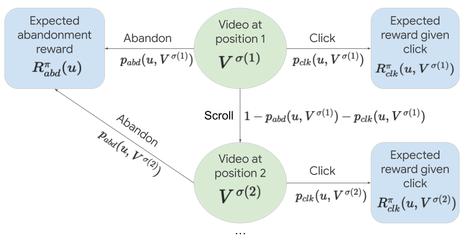
Figure 1. Markov Reward Process with Cascade Click Model

Definition 2.2.

(Cascade Click Model) Given user state $s=(u,V)$, where $u$ represents the user and $V$ represents the set of items, and a ranking order $\sigma$ on $V$, the Cascade model describes how a user interacts with a list of items sequentially. The user’s interaction with the list when inspecting an item is characterized by the following user-item functions:

• $p_{clk}$: A user-item function where $p_{clk}(u,v)$ represents the probability of user $u$ clicking on item $v$ when inspecting it.

• $p_{abd}$: A user-item function where $p_{abd}(u,v)$ represents the probability of user $u$ abandoning the slate when inspecting item $v$.

Taking $(u,V),\sigma,p_{clk},p_{abd}$ as input, the Cascade model defines function $P_{cascade}^{i}$ that outputs the probability the user clicks on the item at the $i$-th position (for $1\leq i\leq n$) with the form:

(1) $$P_{cascade}^{i}(p_{clk},p_{abd},(u,V),\sigma)=\\ \left(\prod_{j=1}^{i-1}(1-p_{clk}(u,V^{\sigma(j)})-p_{abd}(u,V^{\sigma(j)}))\right)\cdot p_{clk}(u,V^{\sigma(i)}).$$

The probability that the user abandons the slate without clicking on any items is defined by the function $P_{cascade}^{0}$ as:

(2) $$P_{cascade}^{0}(p_{clk},p_{abd},(u,V),\sigma)=1-\sum_{i=1}^{n}P_{cascade}^{i}(p_{clk},p_{abd},(u,V),\sigma).$$

Putting everything together, we can rewrite $Q^{\pi}(s,\sigma)$ as

(3) $$R_{abd}^{\pi}(u)+\sum_{i=1}^{n}P_{cascade}^{i}(p_{clk},p_{abd},s,\sigma)\cdot R_{lift}^{\pi}(u,V^{\sigma(i)})$$

We call equation (3) the lift formulation with cascade click model. A natural question is how to order items to maximize $Q^{\pi}(s,\sigma)$ when there is only a single objective. Interestingly, despite the slate nature of this optimization, we prove that the problem can be solved by a user-item ranking function.

Theorem 2.3.

Given user-item functions $p_{clk},p_{abd},R_{abd}^{\pi},R_{lift}^{\pi}$ as input, the optimal ranking for user $u$ on candidate $V$ maximizing $Q^{\pi}((u,V),\sigma)$ for a scalar reward function is to order all items $v\in V$ by $\frac{p_{clk}(u,v)}{p_{clk}(u,v)+p_{abd}(u,v)}\cdot R_{lift}^{\pi}(u,v)$.

Proof.

In equation (3), $R_{abd}^{\pi}(u)$ only depends on users. Therefore, it suffices to optimize $\sum_{i=1}^{n}P_{cascade}^{i}(p_{clk},p_{abd},V,\sigma)\cdot R_{lift}^{\pi}(u,V^{\sigma(i)})$. The rest of the proof follows Theorem 1 in  (Aggarwal et al., 2008). ∎

3. Optimization Algorithm

This section outlines the optimization algorithm for solving Problem 1, initially for the special case of a single objective; i.e., $m=1$ and subsequently extending to multi-objective constraint optimization.

3.1. Single Objective Optimization

Our algorithm employs an on-policy Monte Carlo approach (Sutton and Barto, 2018) which iteratively applies following two steps:

1. Training: Build a function approximation $Q(s,\sigma;\theta)$ for $Q^{\pi}(s,\sigma)$ by separately building function approximations for $R^{\pi}_{abd}$, $R^{\pi}_{clk}$, $p_{clk}$ and $p_{abd}$, using data collected by applying some initial policy $\pi$.

2. Inference: Modify the policy $\pi$ to be $arg\max_{\sigma}Q(s,\sigma;\theta)$ (with exploration).

We outline the main steps in Algorithm 1 and discuss technical details in Section 3.1.1 and  3.1.2.

Algorithm 1 Single objective optimization

  initialize FIFO data buffer $D$

  initialize network $R_{abd}(u,v;\theta)$, $R_{lift}(u,v;\theta)$, $p_{clk}(u,v;\theta)$, $p_{abd}(u,v;\theta)$ parameterized by $\theta$ and initial policy $\pi$

  while 1 do

     Apply $\pi$ to collect $K$ user trajectories and add it into $D$.

     Update $\theta$ by using data $D$ (see Section 3.1.1 for details)

     Update $\pi$ such that for user $u$ with candidate set $V$

1. order $v\in V$ by $\frac{p_{clk}(u,v;\theta)}{p_{clk}(u,v;\theta)+p_{abd}(u,v;\theta)}\cdot R_{lift}(u,v;\theta)$

2. with probability $\epsilon$, promote a random candidate to top

  end while

3.1.1. Training

The training data is collection of user trajectories (see Definition 2.1) stored in $D$. Each user trajectory can be written as $(((u_{0},V_{0}),\sigma_{0},c_{0}),((u_{1},V_{1}),\sigma_{1},c_{1}),\ldots,.)$. We apply gradient updates for $\theta$ with the following loss functions, in sequential order.

Training the abandon reward network

$R_{abd}(u;\theta)$ on abandoned pages with MSE loss function

$$\mathop{\bf E\/}_{\tau\sim D,t\sim[|\tau|]}\left[|R_{abd}(u_{t};\theta)-Reward(\tau,t)|^{2}|c_{t}=0\right]$$

Training the lift reward network

$R_{lift}(u,v;\theta)$ on clicked videos with MSE loss function

$$\mathop{\bf E\/}_{\tau\sim D,t\sim[|\tau|]}[|R_{Lift}(u_{t},V_{t}^{\sigma(c_{t})};\theta)+R_{abd}(u_{t};\theta)-\\ Reward(\tau,t)|^{2}|c_{t}>0]$$

Here we apply the idea from uplift modeling (Gutierrez and Gérardy, 2017) by directly estimating the difference between $R_{clk}^{\pi}(u,v)$ and $R^{\pi}_{abd}(u)$.

Training the click network

on every page with cross-entropy loss function

$$\mathop{\bf E\/}_{\tau\sim D,t\sim[|\tau|]}[-\log(P_{cascade}^{c_{t}}(p_{clk}(\cdot,\cdot;\theta),p_{abd}(\cdot,\cdot;\theta),(u_{t},V_{t}),\sigma_{t}))],$$

using $P_{cascade}^{c_{t}}$ in Definition 2.2.

3.1.2. Inference

Here we simply apply Theorem 2.3 using the function approximation for $p_{clk},p_{abd},R_{abd}^{\pi},R_{lift}^{\pi}$. We randomly promote a candidate to top with small probability as exploration.

3.2. Constraint optimization

When there are multiple objectives, we apply linear scalarization (Roijers et al., 2013) to reduce the constraint optimization problem to a unconstrained optimization problem; i.e., we find weights $w_{2},w_{3},\ldots,w_{m}$ and define the new reward function as $r^{1}+\sum_{i=2}^{m}w_{i}\cdot r^{i}$. With fixed weight combination, we found it often necessary to search new weights when making changes (e.g., add features, change model architecture) to the system, which slows down our iteration velocity. We address the problem by dynamically updating $w$ as part of the training. At a high level, we make the following changes to Algorithm 1:

1. Training: apply Algorithm 1 for $R_{lift}(u,v;\theta)$ as a vector function for all the $m$ objectives separately.

2. Inference: We find a set of weights $w=(1,w_{2},w_{3}\ldots,w_{m})$ and use the following ranking formula at serving time:

   $$\frac{p_{clk}(u,v;\theta)}{p_{clk}(u,v;\theta)+p_{abd}(u,v;\theta)}\cdot\langle R_{lift}(u,v;\theta),w\rangle.$$

   The weights are dynamically updated with offline evaluation.

The algorithm is outlined in Algorithm 2, with details below.

3.2.1. Offline evaluation on exploration candidates

We apply our offline evaluation on a data set consisting of candidates that is randomly promoted as exploration during serving.

Definition 3.1.

We define $D_{eval}$ as

$$\{(u,v,r_{v})|v\in V\text{ and is randomly promoted},((u,V),\sigma,c)\in\tau,\tau\in D,\}$$

Here $r_{v}$ is the reward vector $r((u,V),\sigma)$ if $v$ is clicked and $0^{m}$ otherwise.

We use

$$\mathop{\bf Corr\/}_{(u,v,r_{v})\in D_{eval}}\left(r_{v}^{i},\langle R_{lift}(u,v;\theta),w\rangle\right)$$

as the offline evaluation result for $i$-th objectives. Intuitively, we are computing the correlation between weight-combined lift on $v$ with the immediate rewards from showing $v$. The correlation is computed on exploration candidates to make the evaluation result less biased by the serving policy.

3.2.2. Optimization with correlation constraint

With the offline evaluation defined above, we solve the following problem to update $w$ in Algorithm 2.

Problem 2.

$$\min_{w_{2},w_{3},\ldots,w_{m}}\mathop{\bf E\/}_{(u,v,r)\sim D_{eval}}[\sum_{i=2}^{m}(R_{lift}^{i}(u,v;\theta)\cdot w_{i})^{2}]$$

such that $\mathop{\bf Corr\/}_{(u,v,r_{v})\in D_{eval}}\left(r_{v}^{i},\langle R_{lift}(u,v;\theta),w\rangle\right)\geq\alpha_{i}$ for $i=2,\ldots,m$ and $w=(1,w_{2},\ldots,w_{m})$

Intuitively, we would like to minimize the change to the primary objective while satisfying offline evaluation on secondary objectives.

In the case of a single constraint (i.e., $m=2$), there is a closed-form solution for the problem. To see this, the optimal solution for $w_{2}$ must be either $0$ or be a solution that makes the constraint tight; i.e.,

(4) $$\mathop{\bf Corr\/}\left(r_{v}^{2},R_{lift}^{1}(u,v;\theta)+w_{2}\cdot R_{lift}^{2}(u,v;\theta)\right)=\alpha_{2}.$$

It is not hard to verify that the solution for equation (4) is also the solution for a quadratic equation of $w_{2}$ that can be solved with closed form. Therefore, we can set $w_{2}$ be the best feasible solution from $\{0\}\cup\{\text{solution for equation~{}(\ref{eqn:qudratic}})\}.$

When there is more than one constraint, we found that applying constraints sequentially works well in practice. One can also apply grid search as the offline evaluation can be done efficiently.

Algorithm 2 Constraint Optimization

  initialize FIFO data buffer $D$

  initialize network $R_{abd}(u,v;\theta)$, $R_{lift}(u,v;\theta)$, $p_{clk}(u,v;\theta)$, $p_{abd}(u,v;\theta)$ parameterized by $\theta$ and initial policy $\pi$

  initialize $m$-dimensional weight vectors $w=(1,0,\ldots,0)$.

  while 1 do

     apply $\pi$ and add $K$ user trajectory into $D$.

     update $\theta$ as Algorithm 1

     update $w$ (See Section 3.2.1 and  3.2.2)

     Update $\pi$ such that for user $u$ with candidate set $V$

1. order all $v\in V$ $\frac{p_{clk}(u,v;\theta)}{p_{clk}(u,v;\theta)+p_{abd}(u,v;\theta)}\cdot\langle R_{lift}(u,v;\theta),w\rangle$

2. with probability $\epsilon$, promote a random candidate to top.

  end while

4. Deployment and Evaluation

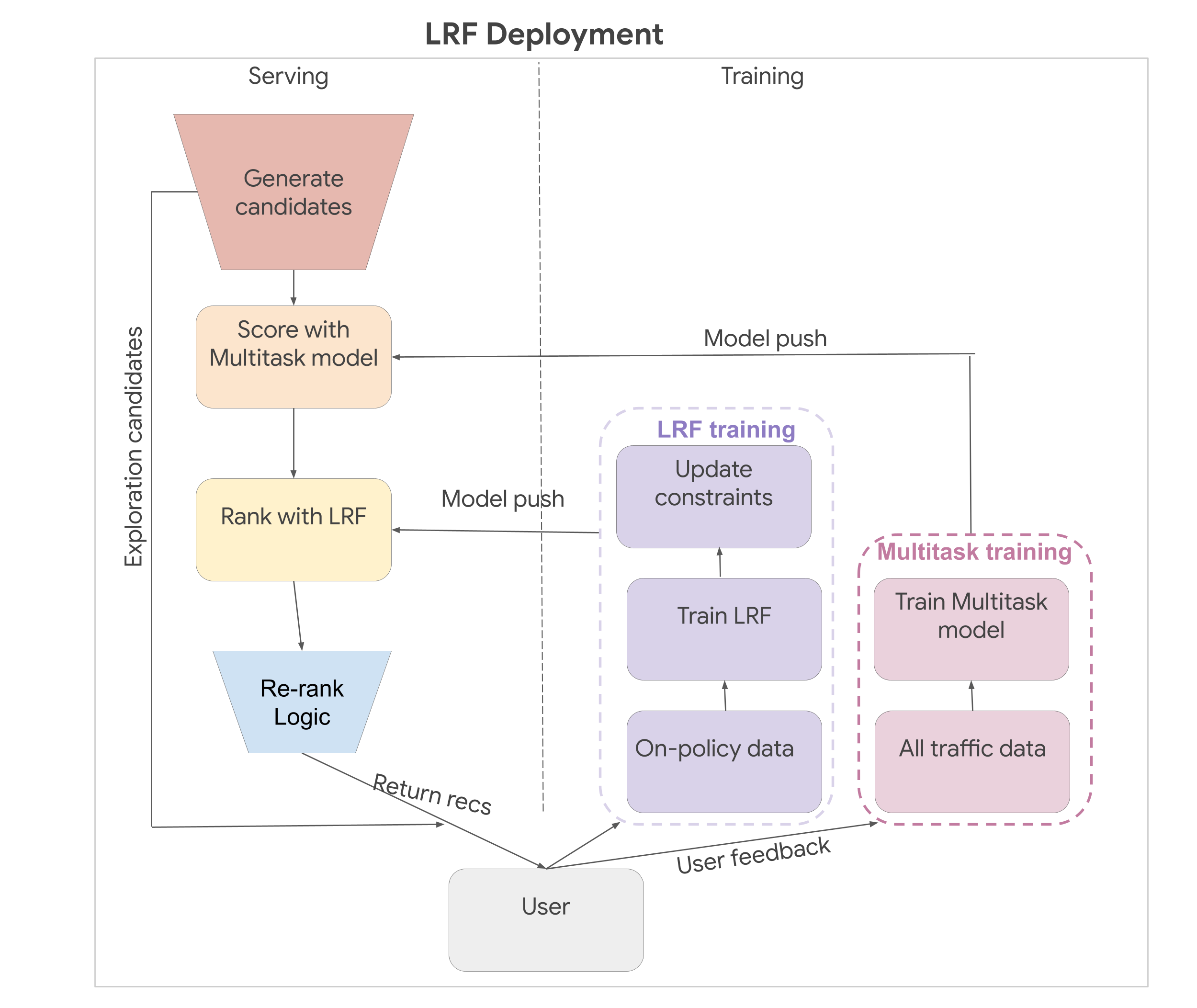
Figure 2. LRF deployment diagram

4.1. Deployment of LRF System

The LRF was initially launched on YouTube’s Watch Page, followed by the Home and Shorts pages. Below we discuss its deployment on Watch Page. Also see illustration in Figure  2.

Lightweight model with on-policy training.

The LRF system applies an on-policy RL algorithm. In order to enable evaluating many different LRF models with on-policy training, we make all LRF model training on a small slice (e.g. 1%) of overall traffic. By doing so,we can compare production and many experimental models that are all trained on-policy together.

Training and Serving.

The LRF system is continuously trained with user trajectories from the past few days. Our primary reward function is defined as the user satisfaction on watches, similar to the metric described in Section 6 of (Christakopoulou et al., 2021). The features include the user behavior predictions from multitask models, user context features (e.g. demographics) and video features (e.g. video topic). We use both continuous features and sparse features with small cardinality. The LRF model comprises small deep neural networks, with roughly $\Theta(10^{4})$ parameters. The inference cost of the model is small due to the size of the model. We use the offline evaluation described in Section 3.2.1 to ensure model quality before pushing to production. At serving time, the LRF takes the aforementioned features as input and outputs a ranking score for all items.

4.2. Evaluation

We conducted A/B experiments for $\Theta(week)$ on YouTube to evaluate the effectiveness of the LRF. Metric trends are shown in Figure 3. Note that first three experiments describe sequential improvements to the production system; the last two experiments ablate certain components of the LRF.

Evaluation Metric

Our primary objective is a metric measuring long-term cumulative user satisfaction; see Sec 6 of (Christakopoulou et al., 2021) for details.

Baseline before LRF Launch:

The previous system uses a heuristic ranking function optimized by Bayesian optimization (Golovin et al., 2017).

Hyperparameters:

We tuned two types of hyperparameters when deploying the LRF: training parameters, such as batch size, are tuned using offline loss; reward parameters, such as constraint weights, are tuned using live experiments.

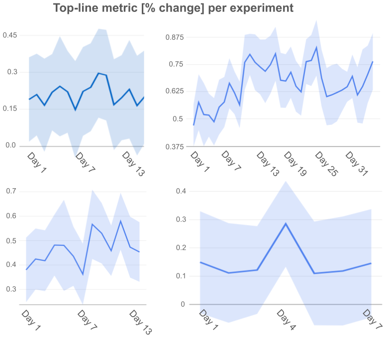
Figure 3. Metrics for experiments in Section 4.2.1(top left), 4.2.2 (top right), 4.2.5 (bottom left), and 4.2.5 (bottom right).

4.2.1. Initial Deployment of LRF

We initially launched a simplified version of the LRF that uses the CTR prediction from the multitask model and ranks all candidates by $CTR\cdot R_{lift}$ . It also uses a set of fixed weights to combine secondary objectives. The control was the previous production system, a heuristic ranking function tuned using Bayesian optimization. The LRF outperformed the production by 0.21% with 95% CI [0.04, 0.38] and was launched to production.

4.2.2. Launch Cascade Click Model

After initial deployment of the LRF, we ran an experiment to determine the efficacy of the cascade click model, i.e., replacing $CTR$ with $\frac{p_{clk}}{p_{clk}+p_{abd}}.$ Adding the cascade click model outperformed the control by 0.66% with 95% CI [0.60, 0.72] in the top-line metric and was launched to production.

4.2.3. Launch Constraint Optimization

We found metric trade-offs between primary and secondary objectives unstable when combining the rewards using fixed weights. To improve stability, we launched the constraint optimization. As an example of the improvement, for the same model architecture change, we saw a $13.15\%$ change in the secondary objective pre-launch, compared to a 1.46% change post-launch. This post-launch fluctuation is considered small for that metric.

4.2.4. Ablating Lift Formulation

To determine the necessity of the lift formula, we ran an experiment that set $R_{abd}$ to be $0$. Such a change regresses top-line metrics by 0.46% with 95% CI [0.43, 0.49]. The metric contributed from watch page recommendations actually increases by $0.2\%$ with 95% CI [0.14, 0.26]. This suggests the importance of lift formulation as it is sub-optimal to only maximize rewards from watch page suggestions.

4.2.5. Two Model Approach

We make separate predictions for $R_{abd}$ and $R_{clk}$. This is also known as the two-model baseline in uplift modelling (Gutierrez and Gérardy, 2017). The ranking formula is then $\frac{p_{clk}}{p_{clk}+p_{abd}}\cdot(R_{click}-R_{abd})$. The experiment results show that our production LRF outperforms this baseline in the top-line metric by 0.12% with 95% CI [0.06, 0.18].

5. Conclusion

We presented the Learned Ranking Function (LRF), a system that combines short-term user-item behavior predictions to optimizing slates for long-term user satisfaction. One future direction is to apply more ideas from Reinforcement Learning such as off-policy training and TD Learning (Sutton and Barto, 2018). Another future direction is to incorporate re-ranking algorithm (e.g., (Wilhelm et al., 2018; Liu et al., 2022)) into the LRF system.

References

- (1)
- met (2019) 2019. Combining online and offline tests to improve News Feed ranking. https://ai.meta.com/blog/online-and-offline-tests-to-improve-news-feed-ranking/
- met (2020) 2020. Efficient tuning of online systems using Bayesian optimization. https://engineering.fb.com/2018/09/17/ml-applications/bayesian-optimization-for-tuning-online-systems-with-a-b-tests/
- Aggarwal et al. (2008) Gagan Aggarwal, Jon Feldman, Martin Pál, and S. Muthukrishnan. 2008. Sponsored Search Auctions for Markovian Users. In Fourth Workshop on Ad Auctions; Workshop on Internet and Network Economics (WINE). http://arxiv.org/abs/0805.0766
- Cai et al. (2023) Qingpeng Cai, Shuchang Liu, Xueliang Wang, Tianyou Zuo, Wentao Xie, Bin Yang, Dong Zheng, Peng Jiang, and Kun Gai. 2023. Reinforcing user retention in a billion scale short video recommender system. In Companion Proceedings of the ACM Web Conference 2023. 421–426.
- Chapelle and Zhang (2009) Olivier Chapelle and Ya Zhang. 2009. A dynamic bayesian network click model for web search ranking. In Proceedings of the 18th international conference on World wide web. 1–10.
- Chen et al. (2019) Minmin Chen, Alex Beutel, Paul Covington, Sagar Jain, Francois Belletti, and Ed H Chi. 2019. Top-k off-policy correction for a REINFORCE recommender system. In Proceedings of the Twelfth ACM International Conference on Web Search and Data Mining. 456–464.
- Christakopoulou et al. (2021) Konstantina Christakopoulou, Can Xu, Sai Zhang, Sriraj Badam, Trevor Potter, Daniel Li, Hao Wan, Xinyang Yi, Elaine Le, Chris Berg, Eric Bencomo Dixon, Ed H. Chi, and Minmin Chen (Eds.). 2021. Reward Shaping for User Satisfaction in a REINFORCE Recommender.
- Covington et al. (2016) Paul Covington, , Jay Adams, and Emrin Sargin. 2016. Deep Neural Networks for YouTube Recommendations. In Proceedings of the 10th ACM Conference on Recommender Systems. New York, NY, USA.
- Craswell et al. (2008) Nick Craswell, Onno Zoeter, Michael J. Taylor, and Bill Ramsey. 2008. An experimental comparison of click position-bias models. In Web Search and Data Mining. https://api.semanticscholar.org/CorpusID:2625350
- Engineering (2023) Pinterest Engineering. 2023. Deep multi-task learning and real-time personalization for closeup recommendations. https://medium.com/pinterest-engineering/deep-multi-task-learning-and-real-time-personalization-for-closeup-recommendations-1030edfe445f
- Golovin et al. (2017) Daniel Golovin, Benjamin Solnik, Subhodeep Moitra, Greg Kochanski, John Karro, and D. Sculley. 2017. Google Vizier: A Service for Black-Box Optimization. In Proceedings of the 23rd ACM SIGKDD International Conference on Knowledge Discovery and Data Mining, Halifax, NS, Canada, August 13 - 17, 2017. ACM, 1487–1495. https://doi.org/10.1145/3097983.3098043
- Gutierrez and Gérardy (2017) Pierre Gutierrez and Jean-Yves Gérardy. 2017. Causal Inference and Uplift Modelling: A Review of the Literature. In Proceedings of The 3rd International Conference on Predictive Applications and APIs (Proceedings of Machine Learning Research), Claire Hardgrove, Louis Dorard, Keiran Thompson, and Florian Douetteau (Eds.), Vol. 67. PMLR, 1–13. https://proceedings.mlr.press/v67/gutierrez17a.html
- Ie et al. (2019) Eugene Ie, Vihan Jain, Jing Wang, Sanmit Narvekar, Ritesh Agarwal, Rui Wu, Heng-Tze Cheng, Tushar Chandra, and Craig Boutilier. 2019. SlateQ: A Tractable Decomposition for Reinforcement Learning with Recommendation Sets. In Proceedings of the Twenty-eighth International Joint Conference on Artificial Intelligence (IJCAI-19). Macau, China, 2592–2599. See arXiv:1905.12767 for a related and expanded paper (with additional material and authors).
- Liu et al. (2022) Weiwen Liu, Yunjia Xi, Jiarui Qin, Fei Sun, Bo Chen, Weinan Zhang, Rui Zhang, and Ruiming Tang. 2022. Neural re-ranking in multi-stage recommender systems: A review. arXiv preprint arXiv:2202.06602 (2022).
- Roijers et al. (2013) Diederik M Roijers, Peter Vamplew, Shimon Whiteson, and Richard Dazeley. 2013. A survey of multi-objective sequential decision-making. Journal of Artificial Intelligence Research 48 (2013), 67–113.
- Sutton and Barto (2018) Richard S Sutton and Andrew G Barto. 2018. Reinforcement learning: An introduction. MIT press.
- Vorotilov et al. (2023) Vladislav Vorotilov, Vladislav Vorotilov, and Ilnur Shugaepov. 2023. Scaling the Instagram explore recommendations system. https://engineering.fb.com/2023/08/09/ml-applications/scaling-instagram-explore-recommendations-system/
- Wilhelm et al. (2018) Mark Wilhelm, Ajith Ramanathan, Alexander Bonomo, Sagar Jain, Ed H Chi, and Jennifer Gillenwater. 2018. Practical diversified recommendations on youtube with determinantal point processes. In Proceedings of the 27th ACM International Conference on Information and Knowledge Management. 2165–2173.
- Yi et al. (2019) Xinyang Yi, Ji Yang, Lichan Hong, Derek Zhiyuan Cheng, Lukasz Heldt, Aditee Kumthekar, Zhe Zhao, Li Wei, and Ed Chi. 2019. Sampling-bias-corrected neural modeling for large corpus item recommendations. In Proceedings of the 13th ACM Conference on Recommender Systems. 269–277.
- Zhang et al. (2022) Qihua Zhang, Junning Liu, Yuzhuo Dai, Yiyan Qi, Yifan Yuan, Kunlun Zheng, Fan Huang, and Xianfeng Tan. 2022. Multi-Task Fusion via Reinforcement Learning for Long-Term User Satisfaction in Recommender Systems. In Proceedings of the 28th ACM SIGKDD Conference on Knowledge Discovery and Data Mining (KDD ’22). ACM. https://doi.org/10.1145/3534678.3539040
- Zhao et al. (2019) Zhe Zhao, Lichan Hong, Li Wei, Jilin Chen, Aniruddh Nath, Shawn Andrews, Aditee Kumthekar, Maheswaran Sathiamoorthy, Xinyang Yi, and Ed Chi. 2019. Recommending what video to watch next: a multitask ranking system. In Proceedings of the 13th ACM Conference on Recommender Systems. 43–51.