Generative Bayesian Modeling with Implicit Priors

Abstract

Generative models are a cornerstone of Bayesian data analysis, enabling predictive simulations and model validation. However, in practice, manually specified priors often lead to unreasonable simulation outcomes, a common obstacle for full Bayesian simulations. As a remedy, we propose to add small portions of real or simulated data, which creates implicit priors that improve the stability of Bayesian simulations. We formalize this approach, providing a detailed process for constructing implicit priors and relating them to existing research in this area. We also integrate the implicit priors into simulation-based calibration, a prominent Bayesian simulation task. Through two case studies, we demonstrate that implicit priors quickly improve simulation stability and model calibration. Our findings provide practical guidelines for implementing implicit priors in various Bayesian modeling scenarios, showcasing their ability to generate more reliable simulation outcomes.

Keywords Bayesian inference  $\cdot$ generative modelling  $\cdot$ prior specification  $\cdot$ data-informed priors  $\cdot$ simulation-based calibration

1 Introduction

The use of model checks in data analysis has been long recognized to constitute good statistical practice (Anscombe and Tukey, 1963; D’Agostino, 1986). In the Bayesian workflow, we often use model-implied data distributions, obtained by marginalizing over the parameter space, as the basis for model checking (Gelman et al., 1996, 2020; Gabry et al., 2019). In order to learn something useful about the model from its marginal data distribution, we not only require a parameter distribution that is proper (as to sample from the model in the first place) but sufficiently sensible in light of the model’s likelihood (Gelman et al., 2017). Once conditioned on data, that is, having obtained the posterior distribution, this is usually not an issue. However, before seeing the data, it requires the careful specification of a sensible prior distribution. Translating domain knowledge into a prior distribution is already a complex task when viewed in isolation (for a historical overview and current challenges see Mikkola et al. (2023)); and still seemingly reasonable choices can produce joint priors with undesirable behaviors that are not easily fixed even in relatively simple models (Aguilar and Bürkner, 2023). A concrete example from one of our case studies is detailed in Figure 1.

In this context, we adopt the term generative modelling to collectively describe techniques for investigating Bayesian models by sampling from them. For example, generative modelling is often employed immediately before/after fitting the model in the form of prior/posterior predictive checks (Gabry et al., 2019), the goal being to understand the information conveyed by the prior and the goodness of fit to the data, respectively. Those assessments, however, have to be done in the context of a specific application. Our interest here lies in addressing challenges faced during earlier stages of model development. That is, before a concrete analysis or application has been conceived, one may nonetheless be interested in understanding when a model, its implementation, and estimation procedure can be relied upon, even in principle.

To this end, one important approach is Simulation-Based Calibration (SBC) (Talts et al., 2020; Modrák et al., 2023). It is a powerful method for highlighting potential problems with Bayesian models, their implementations, and estimation algorithms, but it also come with unique challenges: SBC relies on self-consistency properties of Bayesian models that can only be verified empirically using simulations, hence the name of the approach (see Section 3.5 for details). That is, assessing this property requires that we can sample from the model. The requirement is formally satisfied as long as any proper prior is used, but one is further restricted by computational considerations in practice. For instance, when the prior is too diffuse, draws may exceed the range of standard floating point representations and cause unintended rounding that violates model boundaries (we show this exact problem in our first case study, Section 4.1). This puts one in an awkward situation where one wishes to use a minimally or weakly informative prior (so as to try and assess the model’s performance over as much of its parameter support as possible) but still needs to impose certain constraints to remain within the region of practical computability which, in general, will not map in a straightforward way to the prior specification.

Our goal for this paper is to address the above conundrum, through the following key contributions. (1) We propose a procedure that can be used to iteratively construct a sequence of increasingly informative, implicit priors by preconditioning on small portions of real or simulated data and stopping as soon as a predefined criterion (e.g., computational viability) is reached. These priors are straightforward to implement in any probabilistic programming language and require only small computational overhead. (2) We highlight the connections that such a procedure has to multiple works from the prior elicitation literature. In particular, we are able to leverage formal results therein to establish useful properties that our procedure inherits. (3) We demonstrate the utility of the procedure in two case studies on Bayesian generative modeling.

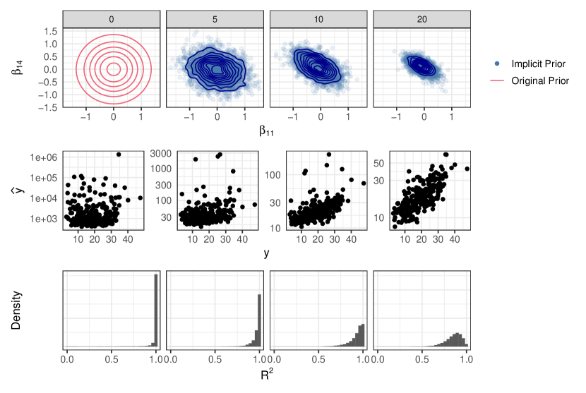
Figure 1: Results from a generalized linear model with gamma likelihood and log-link, using 13 predictors from the same dataset as used in Section 4.1. The columns signify different amounts of preconditioning data used to inform the implicit prior (see Section 3 for details). The plot on the top-left presents the original joint-prior for two of the regression coefficients $\beta_{11}$ and $\beta_{14}$: two independent normal distributions with mean $\mu=0$ and standard-deviation $\sigma=0.5$, a reasonable weakly-informative prior. The rest of the first row presents draws and corresponding contour lines from the implicit priors resulting from conditioning on $5$, $10$, and $20$ observations. By using preconditioning, we can impart different scales, locations and even correlation on the resulting implicit prior, that would be hard to explicitly encode in a probabilistic programming language. The second row compares the observations ($y$) with the corresponding model predictions ($\widehat{y}$) for the original and the three implicit priors. While the original prior is off by up to five orders of magnitude, conditioning on only a few observations quickly reduces the error to only two orders of magnitude for $5$ observations, further improving with growing preconditioning data. The third row presents the implied $R^{2}$ for the original and the preconditioning priors. The original prior puts an unreasonable amount of weight on $R^{2}$ values very close to $1$ (i.e., 100% explained variance), again showcasing how even commonly used reasonable but independent priors can result in completely unreasonable model properties. With growing preconditioning sample sizes this quickly improves, strongly increasing the probability of more reasonable values of $R^{2}$.

2 Related Work

Our core motivation is to find a procedure that produces priors that lead to sensible (at least not too extreme) predictions and whose degree of informativeness is easy to control. Understanding the predictive implications of a given prior is not straightforward (e.g., see Figure 1). Instead, we may invert the process and first come up with an example of what a reasonable dataset would look like, and then fit our model to these "imaginary observations". Even if we started with a noninformative or even improper prior, we can simply add observations until the posterior converges on a region that is sufficiently constrained to avoid major computational difficulties. That posterior can then be used as the new prior for downstream tasks related to generative modelling (see Section 3 for details on our proposed procedure). This approach turns out to be closely related to various methods for constructing data-based priors.

The prototypical idea of deriving a probability distribution from a dataset conceived purely as a thought experiment can be traced back to "the device of imaginary results" from Good (1950)(p. 35) and an explicit interest in methods for eliciting prior distributions seems to have started with Winkler (1967). However, it is with the introduction of the g-prior (Zellner, 1986) that we see one of first thorough discussions of a flexible prior that can be motivated from the perspective of imaginary observations. Specifically, it can be construed as the result of updating an initial vague prior on the parameters of a linear regression model with a set of $N$ observations of the outcome of interest $y$ and a covariate matrix $X$. The ability to control $X$ in turn provides control over the covariance of the resulting joint prior on the model coefficients and we illustrate why this is desirable in Figure 1. More importantly, constructing a prior like this provides a simple way of controlling its informativeness by varying the number of observations that would be used. Because Zellner worked in the conjugate setting, he was able to provide an explicit form where the $g$ hyperparameter (for which the prior is named) scales the covariance matrix. This allows for a finer information adjustment in the prior compared to using whole observations. Although extensions have since been developed (e.g. for the case with more covariates than observations, Maruyama and George (2011); for use in generalized linear models, Sabanés Bové and Held (2011)), we prefer taking an alternative approach that does not depend on having an explicit form for the prior as to strongly widen its generality.

Another angle for obtaining data-based priors is to use power-scaling procedures, which were originally developed in the context of biomedical applications and allow smooth control of the information contained in the prior (Chen et al., 1998; Ibrahim and Chen, 2000; Chen and Ibrahim, 2003). The key motivation for these priors was to incorporate historical data into an analysis, but already in Ibrahim and Chen (2000) it was recognized that in the absence of actual data, "theoretical predictions" from an expert could instead be used. Additionally, although the paper highlighted the conjugate forms that could be achieved for the models it presented, we emphasize that contemporary probabilistic programming languages make it straightforward to implement power scaling in essentially any model for which an explicit likelihood is available (e.g., see Kallioinen et al., 2024). Research on power priors has focused on building a transparent and interpretable framework for elicitation of the hyperparameters. While a clear priority given their relevance for analyses of clinical trial data, we do not expand on those points as they are highly application-specific. The interested reader can consult Ibrahim et al. (2015) for a review.

One point that emerges as a natural concern when using data to construct a prior is the extent to which results will be influenced by the particular realization of data that was used. The expected-posterior (EP) priors of Perez and Berger (2002), although proposed as a method to construct priors for model comparison, can also be regarded as a first attempt to deal with variation in data-based priors. An EP prior is obtained by (1) defining a marginal density for the imaginary observations $y$ (which will be used to construct the prior), (2) taking the posterior that would result from updating the actual inferential model together with $y$, and (3) marginalizing the posterior over themarginal density of $y$. While that procedure removes the dependency on particular realizations of $y$, it does not marginalize over potential covariates $X$ and therefore only partially addresses the problem (Fouskakis et al., 2015). Because the marginalization does not have a closed form in the general setting, handling all sources of variation in imaginary observations inevitably involves increasingly expensive computational approximations. A strand of research has grown around finding procedures to lighten this load, using ideas such as power scaling (Fouskakis et al., 2015), sufficient statistics (Fouskakis, 2019) and Markov chain Monte Carlo model composition (MC³) (Tzoumerkas et al., 2022). We discuss some of these approaches in the context of our procedure and relevant tradeoffs in Section 3.2.

For completeness, we also wish to mention a larger family of approaches that were developed in the context of model comparison via Bayes Factors (BFs). Because BFs involve the ratio of marginal data densities, the quantity is indeterminate unless proper priors are used. This raises the question of how to construct proper priors that are in some sense objective (so as to avoid "biasing" the comparison). We omit a more detailed exploration of the approaches developed under this lens, as they also imply the construction of data-based priors and often have a direct correspondence to the ideas already discussed above. For example, posterior BFs (Aitkin, 1991) simply use all the available data to produce the average of posteriors which would be obtained with each model under consideration. Partial and fractional BFs (O’Hagan, 1995; Gu et al., 2018) essentially correspond to a power scaled version of the same procedure, and intrinsic BFs (Berger and Pericchi, 1996; Moreno and Pericchi, 2014) use the observed data to average over all possible minimal samples that can be constructed from it (i.e. the smallest sample that can be used to obtain a well-defined BF; this was later generalized to consider any data-producing density in Perez and Berger (2002)).

Clearly, the idea of using actual or imaginary observations to obtain data-informed priors has a long and rich history. However, it can be seen that the focus so far has been almost entirely on inferential modeling, where the goal is to obtain posterior inference or metrics for model comparison. In this paper, we instead focus on data-informed implicit priors in the context of generative modeling, as detailed below.

3 Method

Consider a Bayesian model $M_{o}$ with likelihood $p(y\mid\theta)$ and prior $p(\theta\mid\alpha)$, where $y$ denotes the data, $\theta$ the model parameters, and $\alpha$ the prior hyperparameters chosen by the user. Say we would like to generate datasets $\tilde{y}$ from $M_{o}$ before conditioning on any data. If the prior $p(\theta\mid\alpha)$ is proper, we can do this by drawing datasets from the model’s prior predictive distribution.

$$\tilde{y}\sim p(y\mid\alpha)=\int_{\theta}p(y\mid\theta)\,p(\theta\mid\alpha)\,d\theta.$$ (1)

Of particular interest for this paper is how weakly informative priors can cause serious problems for the assessment of posterior calibration, as we illustrate in Section 4. At the same time, defining priors that properly represent our prior knowledge is exceedingly complicated (Mikkola et al., 2023). This makes the sole dependence of the prior predictive on $\alpha$ problematic, as choosing good values for $\alpha$ is both important and hard (Gabry et al., 2019; Gelman et al., 2020).

Rather than trying to encode all our prior knowledge via $p(\theta\mid\alpha)$ directly, we supply a dataset $y_{c}$ to $M_{0}$ as an additional source of information. As we will show, even if $y_{c}$ is small, this can greatly help in reducing the probability of simulating unreasonable data from the model’s preconditioned prior predictive. We will discuss potential sources for $y_{c}$ in Section 3.3 and its required size in Section 3.4. For now, let us assume we have already obtained a suitable dataset $y_{c}$.

By means of Bayesian updating we can use $y_{c}$ to update the original prior as

$$p(\theta\mid\alpha,y_{c})=\frac{p(\theta\mid\alpha)\,p(y_{c}\mid\theta)}{p(y_{c})}.$$ (2)

This results in what we call the preconditioned model $M_{c}$, which uses the same likelihood distribution $M_{0}$ but with an updated prior $p(\theta\mid\alpha,y_{c})$. After updating, rather than drawing samples from the original prior predictive $p(y\mid\alpha)$, we can instead draw datasets from the posterior predictive of $M_{c}$, which now depends on both $\alpha$ and $y_{c}$:

$$\tilde{y}\sim p(y\mid y_{c},\alpha)=\int_{\theta}p(y\mid\theta)\,p(\theta\mid\alpha,y_{c})\,d\theta$$ (3)

The benefit of this approach is that, in many cases, it will be easier to reason about data than it is to reason about potentially high-dimensional prior hyperparameter vectors.

In practice, we do not have direct access to the updated prior $p(\theta\mid\alpha,y_{c})$ because it is not available analytically, except for the few special cases where likelihood and prior are conjugate. Accordingly, we have to fall back to approximate inference algorithms, such as MCMC, that provide us with a set of $S$ draws $\theta_{c}^{(s)}$ from $p(\theta\mid\alpha,y_{c})$. These draws constitute an implicit (non-analytic) representation of the prior $p(\theta\mid\alpha,y_{c})$, meaning we can use the samples $\theta_{c}^{(s)}$ to simulate data from the posterior predictive given $y_{c}$ by sampling from $p(y\mid\theta_{c}^{(s)})$ but cannot directly utilize them to represent the prior in most probabilistic programming languages. The reason is that these languages typically require an analytic expression of all the involved probability densities (Stan Development Team, 2024a; Abril-Pla et al., 2023; Ge et al., 2018). We could, of course, attempt to resolve this by fitting a parametric distribution (e.g., multivariate normal) to the draws $\theta_{c}^{(s)}$, but the bias resulting from this parametric approximation may be severe and generally hard to quantify, so we prefer working with the draws $\theta_{c}^{(s)}$ directly. However, doing so poses practical challenges for common Bayesian simulation procedures such as SBC; challenges that we will elaborate and subsequently resolve in Sections 3.5 and 3.6.

3.1 Distributions over preconditioning datasets

In the previous section, we assumed the existence of a single, fixed preconditioning dataset $y_{c}$ with corresponding implicit prior $p(\theta\mid\alpha,y_{c})$. Instead, we may prefer to think about a preconditioning data-generating process instead of a specific dataset, to reduce the potential of dataset-specific artifacts affecting our conclusions. That is, we may think of any individual dataset $y_{c}$ as being drawn from an (implicit or explicit) data-generating distribution $p(y_{c})$. In fact, we can extend the preconditioned prior $p(\theta\mid y_{c},\alpha)$ by integrating over $p(y_{c})$ to obtain

$$p_{c}(\theta\mid\alpha):=\int_{y_{c}}\,p(\theta\mid\alpha,y_{c})\,p(y_{c})\,d\theta\,dy_{c},$$ (4)

where we use the subscript $c$ to distinguish $p_{c}(\theta\mid\alpha)$ from the original prior $p(\theta\mid\alpha)$. The marginal preconditioned prior $p_{c}(\theta\mid\alpha)$ also implies a corresponding prior predictive:

$$\tilde{y}\sim p_{c}(y\mid\alpha):=\int_{y_{c}}p(y\mid y_{c},\alpha)\,p(y_{c})\,dy_{c}=\int_{y_{c}}\int_{\theta}p(y\mid\theta)\,p(\theta\mid\alpha,y_{c})\,p(y_{c})\,d\theta\,dy_{c}$$ (5)

Both the marginal preconditioned prior and prior predictive are implicit in several ways: (1) $p(\theta\mid\alpha,y_{c})$ is implicit and only represented via draws (see above); (2) $p(y_{c})$ is also often only implicitly given via a resampling or bootstrapping procedure on real data (see Section 3.3); and (3) even if both of these distributions were explicit, the integrals in Equations (4) and (5) are not in general analytically solvable, outside of simple cases that are of limited practical interest.

As such, we have to rely on a sampling-based representation: When taking a number of $T$ preconditioning datasets $y_{c}^{(t)}$ from $p(y_{c})$ (each of size $N$), we obtain $T$ corresponding preconditioned models $M_{c}^{(t)}$, $t=1,\ldots,T$, which in turn imply a collection of $T$ implicit priors $p(\theta\mid\alpha,y_{c}^{(t)})$. When sampling $S$ draws $\theta_{c}^{(s)}$, $s=1,\ldots,S$, from each of the $p(\theta\mid\alpha,y_{c}^{(t)})$ priors, and sampling one dataset $\tilde{y}^{(s,t)}$ for each combination of $s$ and $t$, we obtain $S\times T$ simulated datasets. Importantly, due to the preconditioning procedure, each dataset $\tilde{y}^{(s,t)}$ generated this way is living in a narrower space than is the case for datasets sampled directly from the original (often problematically wide) prior predictive $p(y\mid\alpha)$. At the same time, we avoid overly relying on any single such narrower space, as would be the case if we just considered a single preconditioning dataset.

3.2 Representative preconditioned priors

Above, we discussed that, for a given $y_{c}$, the preconditioned prior $p(\theta\mid\alpha,y_{c})$ can be seen as an instance of a whole distribution of priors implied by the distribution over preconditioning datasets $p(y_{c})$. This then leads to the concept of a "marginal" preconditioned prior that we obtained by integrating $p(\theta\mid\alpha,y_{c})$ over $p(y_{c})$. Here, we want to add a complementary viewpoint by showing that each $p(y\mid\alpha,y_{c})$ can be seen an approximation of a single "representative" preconditioned prior.

Let us denote preconditioning datasets consisting of $N$ observations as $y_{c,N}$. Further, let $p(y_{c,N}\mid\theta)^{\tau}$ be the power likelihood (also known as tempered or fractional likelihood) with scaling factor $\tau>0$ (O’Hagan, 1995; Ibrahim and Chen, 2000; Bhattacharya et al., 2019; Kallioinen et al., 2024). Increasing $\tau>1$ will increase the influence of the likelihood on the posterior, while $0<\tau<1$ will decrease the influence, relative to the non-weighted $\tau=1$ case. Suppose, we have a preconditioning dataset of size $N$ but want it to have a weight on the posterior comparable to a preconditioning dataset of size $M$. We can express this as a power-scaled likelihood with scaling factor $\tau=M/N$, since this implies a weight of $M/N$ for the log-likelihood:

$$p(y_{c,N}\mid\theta)^{M/N}\Leftrightarrow M/N\log p(y_{c,N}\mid\theta)$$ (6)

Remember that, by means of preconditioning, our goal is to reduce the entropy of the joint prior just enough for it to imply a sufficiently sensible model-implied data distribution. But we also don’t want to make the prior too informative (see also Section 3.4). Say, we think that using $M$ observations for preconditioning strikes the right balance in that regard. Then, for given $y_{c,N}$, we set

$$p_{M}(\theta\mid\alpha,y_{c,N}):=\frac{p(\theta\mid\alpha)\,p(y_{c,N}\mid\theta)^{M/N}}{\int_{\theta}p(\theta\mid\alpha)\,p(y_{c,N}\mid\theta)^{M/N}\,d\theta},$$ (7)

as the preconditioned power prior that results from the power likelihood $p(y_{c,N}\mid\theta)^{M/N}$ and the original prior $p(\theta\mid\alpha)$. For a comprehensive review on power priors, see Ibrahim et al. (2015). The preconditioned power prior contains information equivalent to $M$ observations. However, for finite $N$, it depends on $y_{c,N}$ and as such is not necessarily unique. That said, we can define a (unique) representative preconditioned prior as the limiting distribution of $p_{M}(\theta\mid\alpha,y_{c,N})$, as $N$ goes to infinity:

$$p_{M}(\theta\mid\alpha,y_{c,\infty}):=\lim_{N\rightarrow\infty}p_{M}(\theta\mid\alpha,y_{c,N}).$$ (8)

For this definition to make sense, we need to know that the limit exists, i.e., that $p(\theta\mid\alpha,y_{c,N})$ converges to the same stationary (point) distribution regardless of the exact values the series $(y_{c,N})_{N=1}^{\infty}$ takes on. Clearly, this requirement will be fulfilled for any model for which a Bernstein–von Mises-type theorem holds, so it is not in fact very restrictive. However, as opposed to the usual cases in which Bernstein–von Mises is applied, the limiting distribution $p_{M}(\theta\mid\alpha,y_{c,\infty})$ is not, in general, a point distribution (i.e., it remains to have positive entropy) and still depends on the prior hyperparameters $\alpha$. Intuitively, this is can be understood as follows: Independently of $N$, the power-scaled likelihood $p(y_{c,N}\mid\theta)^{M/N}$ has a total weight equivalent to only $M$ unweighted observations, which cannot fully overcome the prior as long as $M$ remains finite.

The representative preconditioned prior is non-analytic, except perhaps for some conjugate special cases. That said, we can approximate it infinitely well by choosing a very large $N$ for $y_{c,N}$ and then evaluating $p_{M}(\theta\mid\alpha,y_{c,N})$, say, via MCMC. However, because of the large amounts of data we have to condition on, this approach can be very slow and thus impractical Bardenet et al. (2017). What is more, if we use real data as the preconditioning dataset, the amount of available data may be too small to approximate the limiting distribution with sufficient accuracy. For both of these reasons, we believe it as generally more practical to follow the approach from Section 3.1 of using several preconditioning datasets of actual size $M$: From the total weight argument above, we can see that every prior $p(\theta\mid\alpha,y_{c,M})$ obtained from a given preconditioning dataset $y_{c,M}$ of $M$ observations can be understood as an approximation of $p_{M}(\theta\mid\alpha,y_{c,\infty})$. Accordingly, by selecting a set of $T$ datasets $y_{c,M}^{(t)}$ all consisting of $M$ observations, we are in fact exploring the prior space centered around the expected preconditioned prior $p_{M}(\theta\mid\alpha,y_{c,\infty})$. Notably, while the marginal preconditioned prior from Equation (4) contains the variation encoded in $p(y_{c,M})$, the representative preconditioned prior removes said variation.

3.3 Origin of the preconditioning data

The exact properties of the datasets $\tilde{y}$ simulated from an implicit prior $p(\theta\mid\alpha,y_{c})$ are determined by the choice of preconditioning data $y_{c}$. Accordingly, we need to think carefully about how to obtain said data. Perhaps the most immediate source is an already available real dataset whose properties we would like to encode in the implicit prior. In this context, it is highly important to consider the intended use-case of the implicit prior: Do we want to use it (a) as an actual prior in a real-world data analysis or (b) only as a generative prior to stabilize Bayesian simulations?

If the goal is to obtain a prior for a real-world analysis, then care must be taken not to double dip into the current data to be analysed. That is, to avoid conditioning on the same observations twice, once when creating the implicit prior and once more when performing the actual posterior inference on the full dataset. Instead, to safely use real data for this goal, they should not be the same data we want to perform inference on. Possible sources are past studies related to the current data (historical data; (Schmidli et al., 2014; Ibrahim et al., 2015)) or data from other domains that we expect to behave similarly to the current data. The more similar the data source is to the data we want to analyze, the higher the chance for the implicit prior to represent the same properties. For example, in medical randomized controlled trials, it is not uncommon to use data from placebo groups of previous trials to inform the priors for the new trial (Hall et al., 2021). If the goal of the implicit prior is rather to provide a more reliable investigation of a proposed model via Bayesian simulations, without applying it in the actual data analysis that may follow, then the same real data may be readily used both for constructing the implicit prior and for the actual data analysis (see also Section 3.6 for more details on this use-case).

In any case, once we have obtained our real dataset and declared it safe for use in preconditioning, we can draw $T$ preconditioning datasets of desired size by simply subsetting the available data. This can be done deterministically, completely at random or through a more advanced bootstrapping scheme (Ren et al., 2010). Each of the individual datasets $y_{c}^{(t)}$ drawn that way results in one sample $p(\theta\mid\alpha,y_{c}^{(t)})$ from the distribution of implicit priors $p_{c}(\theta\mid\alpha)$, as discussed in Section 3.1.

Using real data is not the only option to obtain suitable preconditioning datasets $y_{c}$. Alternatively, one may simulate suitable datasets from a data-generating process that may or may not resemble the assumed data-generating process of $M_{o}$ (see below). We motivated the use of implicit priors with the argument that it is very hard to choose hyperparameter configuration such that the prior $p(\theta\mid\alpha)$ implies realistic data via its prior predictive distribution $p(y\mid\alpha)$. It is usually much easier to choose a single (or a few) parameter configuration(s) such that $p(y\mid\theta)$ yields realistic data. However, choosing individual parameter configurations does not directly translate into a sensible and computational viable prior over the parameter space. This is where the idea of simulated preconditioning data comes into play.

Let us first assume that we simulate $y_{c}$ directly from the likelihood $p(y\mid\theta)$ of our model of interest $M_{o}$. This makes sense if we believe that likelihood to be a good representation of reality with interpretable parameters $\theta$ that have meaning to the analyst. In such a case, we can choose fixed parameter configurations $\theta_{c}$ and then draw $y_{c}\sim p(y\mid\theta_{c})$. If $y_{c}$ is not too small, this approach will center the implicit prior around (a function of) $\theta_{c}$ in expectation, assuming identifiability of $\theta$. The parameter configuration $\theta_{c}$ may be chosen either with the goal in mind to creating "typical" data for a given scenario or it may be chosen to represent a given (null) hypothesis whose influence on the posterior we want to strengthen. To make this more concrete, consider a randomized control trial of a medical treatment with parameter $\delta$ that quantifies the treatment effect, accompanied by a set of other parameters $\beta$ (e.g., baseline values, effects of control variables etc.), together making up $\theta=(\delta,\beta)$. Suppose we know that, for similar treatments, the treatment effect has been about $\delta=0.3$ on average (on some standardized scale understood by the analyst). If we wanted to convey this information in the form of an implicit prior, we would set $\delta_{c}=0.3$, choose the values for $\beta_{c}$ accordingly, and finally generate preconditioning data $y_{c}\sim p(y\mid\delta_{c},\beta_{c})$. If instead we wanted to convey the null hypothesis of no treatment effect via an implicit prior, we would set $\delta_{c}=0$ and proceed as above. This can be understood almost like an implicit version of penalized complexity priors (Simpson et al., 2017), where substantial prior mass is put in the neighbourhood of a parameter configuration implying a simpler sub-model (e.g., a sub-model assuming no treatment effect).

Some models do not have interpretable parameters, thus making it hard to even choose a single, sensible parameter configuration $\theta_{c}$. This often holds for flexible, highly parameterized models such as polynomial models, generalized additive models, or neural networks. Often these models are used as surrogates of more realistic and interpretable but hard-to-evaluate models (Alizadeh et al., 2020). This includes models represented via non-analytic differential equations for which only a simulator is available making it hard to perform posterior inference (Cranmer et al., 2020). Denoting the simulator as $p_{\text{sim}}(y\mid\psi)$ with parameters $\psi$, we would use the simulator’s interpretability to specify a "typical" (or null hypothesis) configuration $\psi_{c}$. Subsequently, we would sample $y_{c}\sim p_{\text{sim}}(y\mid\psi)$ and use it to obtain an implicit prior $p(y\mid\alpha,y_{c})$ for the model $M_{o}$ actually under evaluation.

3.4 Size of preconditioning data

The properties of the preconditioned priors not only depends on the origin of the preconditioning dataset but also its size. In the context of model comparison, if the original prior $p(\theta\mid\alpha)$ is improper, Berger and Pericchi (1996) suggest to find a dataset $y_{c,N}$, consisting of $N$ observations, such that the resulting preconditioned prior is proper, i.e., for which the implied marginal likelihood is finite:

$$p(y_{c,N}\mid\alpha)=\int_{\theta}p(y_{c,N}\mid\theta)\,p(\theta\mid\alpha)\,d\theta<\infty$$ (9)

In this context, a dataset $y_{c,N}$ would be called minimal if none of its subsets $y_{c,N^{\prime}}\subset y_{c,N}$ with $N^{\prime}<N$ implies a proper prior. Starting from an improper prior, Berger and Pericchi (1996) observe that the minimal $N$ will often be equal to or less than the number of parameters $\theta$. At least in simple models, this $N=\text{dim}(\theta)$ heuristic makes all model parameters identifiable, so it can serve as a good starting point. In the case of a prior that is already proper before preconditioning, an empty dataset is already minimal, but the generated prior-predicted data could still be completely unreasonable. Thus, it is necessary but not sufficient for the preconditioning dataset to imply a proper prior. In our case studies, we found that the $N=\text{dim}(\theta)$ heuristic still provides a reasonable starting point even for proper yet wide priors. That said, with growing model complexity and a mix of proper and improper priors, the (effective) number of parameters in a model is not an obvious property that we can simply read of the model definition (Bürkner et al., 2023).

To illustrate the amount of data required, imagine transitioning through the space of increasingly informative priors, from vague to narrow: Starting from improper flat priors, we would need enough data to update to minimal proper priors to be able to sample from them at all. However, proper priors can have wide tails, such as a Student-t distribution with low degrees of freedom, which easily lead to extreme datasets. To prevent the worst extremes, we will have to update further to the point of at least having the first few finite moments, eventually reaching weakly informative priors. Combining multiple weakly informative priors (of individual parameters) can still lead to extreme datasets (Gabry et al., 2019); see also Figure 1. As a remedy, we need need to remove enough of the tails from our prior and encode parameter dependencies until the joint prior starts producing reasonable datasets. The amount of data required will differ, depending on where you start this journey, say with flat or weakly informative priors. Similarly, the model itself will influence how much data is necessary. We show examples of the scaling with different preconditioning dataset sizes in our case studies in Section 4.

The above considerations apply for finding a dataset $y_{c}$ of roughly minimal size, at which the data predicted from the implicit prior become sufficiently realistic with high probability. Such priors will likely remain rather weakly informative. One may also build more informative implicit priors based on larger preconditioning datasets. Starting from a very wide, uninformative base prior $p(\theta\mid\alpha)$, the weight of an implicit prior $p(\theta\mid\alpha,y_{c},y_{r})$ can be quantified by its sample size relative to the sample size of the real data $y_{r}$ being analyzed. For example, if $y_{c}$ was of size $50$ and $y_{r}$ of size $100$, we could infer that the weight of the implicit prior in determining the final posterior $p(\theta\mid\alpha,y_{c})$ would be about $50/(50+100)=1/3$. This may be understood as a generalization of the conjugate beta-binomial model for binary data, where the two shape parameters $(\alpha_{1},\alpha_{2})$ of the beta prior can be interpreted as a dataset of size $\alpha_{1}+\alpha_{2}$ whose information is exactly equivalent to the information contained in the prior (Gelman et al., 2013).

3.5 Simulation-Based Calibration

One important procedure building on Bayesian simulations is simulation-based calibration (SBC). In a nutshell, the aim of SBC is to test the goodness of posterior approximations by exploiting general self-consistency properties of Bayesian models. Here, we shortly review SBC to subsequently extend it to our implicit priors framework. For a comprehensive introduction, including more theoretical background, please refer to Modrák et al. (2023) and Talts et al. (2020).

Practically, SBC starts with a model $M_{o}$ whose correct implementation and posterior estimation we want to check. For this purpose, we generate $J$ datasets $\tilde{y}^{(j)}$ ($j=1,\ldots,J$, each of fixed size $N$) from the model’s prior predictive distribution. Thereby, each individual dataset is simulated on the basis of a corresponding parameter draw $\theta_{o}^{(j)}$ from the prior $p(\theta\mid\alpha)$, such that we know the mapping between dataset $\tilde{y}^{(j)}$ and its generating parameter draw $\theta_{o}^{(j)}$. Using a posterior approximation algorithm whose correctness we seek to check, $M_{o}$ is then fitted to each of the datasets $\tilde{y}^{(j)}$, resulting in $J$ models $M^{(j)}$, with respective approximate posteriors $p_{a}(\theta\mid\alpha,y^{(j)})$, each represented by a set of $S$ posterior draws $\theta^{(j,s)}$. Using $\theta^{(j)}_{o}$ as the known ground truth, we can calculate a rank statistic for each univariate posterior quantity $f(\theta)$ (e.g., a specific parameter) by counting the number of posterior draws $f(\theta^{(j,s)})$ that are smaller than $f(\theta^{(j)}_{o})$:

$$R^{(j)}:=\sum^{S}_{s=1}\mathbb{I}[f(\theta^{(j,s)})<f(\theta^{(j)}_{o})]$$ (10)

This results in a single rank-value per model $M^{(j)}$ and a distribution of ranks across all $J$ models. If the approximate posteriors $p_{a}(\theta\mid\alpha,\tilde{y}^{(j)})$ are, in fact, resembling the corresponding true posteriors $p(\theta\mid\alpha,\tilde{y}^{(j)})$, the distribution of ranks $R$ per parameter is discretely uniform for every $f$. This property can be used to assess the correctness of the posterior approximation by testing the rank distribution for uniformity. If uniformity is not given, this indicates a problem in the model simulator, model implementation, or posterior approximation algorithm (or in multiple of these components).

One graphical uniformity test we want to highlight here computes simultaneous confidence bands for the empirical cumulative distribution function (ECDF) of the rank distribution under the assumption of uniformity (Säilynoja et al., 2022). We use these in Figures 2 and 5, where uniformity can be rejected in cases where the ECDF lies outside the 95% confidence level bands of the theoretical CDF. The corresponding (frequentist) test statistic is the probability $\gamma$ of observing the most extreme point on the ECDF under the assumption of uniformity:

$$\gamma=2\underset{j\in\{1,...,J+1\}}{\mathrm{min}}\left(\mathrm{min}\{\mathrm{Bin}(R_{j}\mid J,z_{j}),1-\mathrm{Bin}(R_{j}-1\mid J,z_{j})\}\right),$$ (11)

Here, $z_{j}=\frac{j}{J+1}$ is the expected proportion of ranks below $j$, $R_{j}$ is the actual (empirical) number of ranks below $j$, and $\mathrm{Bin}(R\mid J,p)$ is the CDF of the binomial distribution with $J$ trials and a probability of success of $p$, evaluated at $R$. The calculated $\gamma$-score (or its logarithm) can be then be compared to a threshold value corresponding to a given confidence level to reject uniformity, such as shown in Figure 3 (for more details see Säilynoja et al., 2022). The entire process of traditional SBC is also summarized in Algorithm 1.

Algorithm 1 Traditional SBC

$M_{o}$ $\triangleright$ Choose a model for which to perform SBC

$J>0$ $\triangleright$ Choose number of SBC simulations

for $j\text{ in }1:J$ do

     Draw $\theta_{o}^{(j)}$ from $p(\theta\mid\alpha)$ $\triangleright$ Draw prior sample

     Draw $\tilde{y}^{(j)}$ from $p\left(y\mid\theta_{o}^{(j)}\right)$ $\triangleright$ Draw SBC dataset

     $M^{(j)}\leftarrow$ fit($M_{o}$, $\tilde{y}^{(j)}$) $\triangleright$ Fit SBC model

     Draw $\theta^{(j,s)}$ from $p_{a}(\theta\mid\alpha,\tilde{y}^{(j)})$ $\triangleright$ Obtain $S$ posterior draws from $M^{(j)}$

     $R^{(j)}\leftarrow\sum^{S}_{s=1}\mathbb{I}[f(\theta^{(j,s)})<f(\theta^{(j)}_{o})]$ $\triangleright$ Calculate rank statistic

end for

Test $(R^{(1)},\ldots,R^{(J)})$ for uniformity

3.6 SBC with implicit priors

Traditional SBC does not immediately work with the introduced preconditioned priors. This is because, for the self-consistency properties of SBC to hold, the priors used in the model simulator and the model implementation need to be the same. When using a preconditioned prior $p(\theta\mid\alpha,y_{c})$ in the simulator in combination with a model implementation that still contains the original prior $p(\theta\mid\alpha)$, the self-consistency property is broken. This may lead to SBC results that appear to indicate miscalibration even though all aspects of the model (simulator, implementation, approximator) are in fact correct. Of course, self-consistency can, in theory, be restored by also using the preconditioned prior in the model implementation. This however faces the challenge of properly translating the preconditioned prior draws into an appropriate analytic prior density to be understood by common probabilistic programming languages. Since this approach is not generally viable, we have to look for alternatives.

The posterior $p(\theta\mid\alpha,y_{c},\tilde{y}^{(j)})$ implied by fitting the preconditioned model $M_{c}$ on the $j$th SBC dataset $\tilde{y}^{(j)}$ can be written in two equivalent ways. First, as a two-step procedure in which we (i) update the original prior with preconditioning data and subsequently (ii) update the preconditioned prior with the SBC data $\tilde{y}^{(j)}$. Second, as a single-step Bayesian updating of the original prior $p(\theta\mid\alpha)$ with the joint data $(y_{c},\tilde{y}^{(j)})$:

$$p(\theta\mid\alpha,y_{c},\tilde{y}^{(j)})\propto p(\theta\mid\alpha)\,p(y_{c}\mid\theta)\,p(\tilde{y}^{(j)}\mid\theta)=p(\theta\mid\alpha)\,p(y_{c},\tilde{y}^{(j)}\mid\theta)$$ (12)

For the equality to hold, we only require conditional independence of $y_{c}$ and $\tilde{y}^{(j)}$ given $\theta$, which is always true by construction of the preconditioned prior. Informally speaking, if the data can be written in rectangular fashion, the single-step approach is nothing else than concatenation the observations in $y_{c}$ with those in $\tilde{y}^{(j)}$ and passing the joint dataset $(y_{c},\tilde{y}^{(j)})$ to the model implementation.

We can further generalize this SBC procedure by not only working with a single preconditioning dataset but with a set of $T$ such datasets $y_{c}^{(t)}$ (see also Section 3.1). Suppose we now simulate $J$ SBC datasets per preconditioning dataset, then we end up with $T\times J$ rank statistics to be tested for uniformity, either jointly or separately for each $t=1,\ldots,T$. Using Bayesian updating, the $T\times J$ SBC posteriors can be obtained as

$$p(\theta\mid\alpha,y_{c}^{(t)},\tilde{y}^{(j)})\propto p(\theta\mid\alpha)\,p(y_{c}^{(t)}\mid\theta)\,p(\tilde{y}^{(j)}\mid\theta)\propto p(\theta\mid\alpha)\,p(y_{c}^{(t)},\tilde{y}^{(j)}\mid\theta).$$ (13)

The adapted process of SBC using implicit priors is summarized in Algorithm 2. As we want to show the general principle, we refrained from including all details such as properly weighting observations for the power-scaling approach. Compared to traditional SBC, this procedure has the overhead costs of (a) fitting the $T$ preconditioned models $M_{c}^{(t)}$, one for each $y_{c}^{(t)}$, and (b) fitting the SBC models not just on $\tilde{y}^{(j)}$ but on the joint data $(y_{c}^{(t)},\tilde{y}^{(j)})$. Since the $y_{c}^{(t)}$ is supposed to be small, both in absolute terms and relative to the $\tilde{y}^{(j)}$, these overhead costs are usually negligible. In fact, we may even see a speedup of the whole SBC procedure since fitting models based on extreme datasets $\tilde{y}^{(j)}$ from the original prior may be much slower than fitting models on $(y_{c}^{(t)},\tilde{y}^{(j)})$ obtained in the implicit priors SBC approach; even if the latter datasets are slightly larger.

Algorithm 2 SBC with implicit priors

$M_{o}$ $\triangleright$ Choose a model for which to perform SBC

$y_{c}^{(t)}$ for $t=1,\ldots,T$ $\triangleright$ Choose preconditioning datasets

$J>0$ $\triangleright$ Choose number of SBC simulations per dataset

for $t\text{ in }1:T$ do

     $M_{c}^{(t)}\leftarrow$ fit($M_{o}$, $y_{c}^{(t)}$)

     for $j\text{ in }1:J$ do

         Draw $\theta_{c}^{(j)}$ from $p_{a}(\theta\mid\alpha,y_{c}^{(t)})$ $\triangleright$ Draw preconditioned prior sample

         Draw $\tilde{y}^{(j)}$ from $p\left(y\mid\theta_{c}^{(j)}\right)$ $\triangleright$ Draw SBC dataset

         $M^{(j)}\leftarrow$ fit($M_{o}$, $(y_{c}^{(t)},\tilde{y}^{(j)})$) $\triangleright$ Fit SBC model

         Draw $\theta^{(j,s)}$ from $p_{a}(\theta\mid\alpha,y_{c}^{(t)},\tilde{y}^{(j)})$ $\triangleright$ Obtain $S$ posterior draws from $M^{(j)}$

         $R^{(t,j)}\leftarrow\sum^{S}_{s=1}\mathbb{I}[f(\theta^{(j,s)})<f(\theta^{(j)}_{c})]$ $\triangleright$ Calculate rank statistic

     end for

end for

Test $(R^{(1,1)},\ldots,R^{(T,J)})$ for uniformity

3.7 Implicit priors for selected parameters

So far, we have only considered the case where the preconditioning data $y_{c}$ creates an implicit prior for all parameters $\theta$. However, in some scenarios, it might be desirable to split $\theta=(\theta_{I},\theta_{U})$ and only inform a subset of parameters $\theta_{I}$ while leaving the remaining parameter $\theta_{U}$ uninformed by the preconditioning data. For example, in a regression model, we might want to update the prior for all predictors’ regression coefficients while leaving the intercept uninformed. In order to obtain data-simulations $\tilde{y}$ for this case, we need to amend Equation (3) to obtain

$$\tilde{y}\sim p(y\mid y_{c},\alpha)=\int_{\theta_{U}}\int_{\theta_{I}}p(y\mid\theta_{I},\theta_{U})\,p(\theta_{I}\mid\alpha,y_{c})\,p(\theta_{U}\mid\alpha)\,d\theta_{I}\,d\theta_{U},$$ (14)

where $p(\theta_{U}\mid\alpha)$ is the original prior for $\theta_{U}$ (before preconditioning) and $p(\theta_{I}\mid\alpha,y_{c})$ is obtained from the full preconditioned prior $p(\theta\mid\alpha,y_{c})=p(\theta_{I},\theta_{U}\mid\alpha,y_{c})$ by marginalizing out $\theta_{U}$.

Despite the more complex form of the predictive distribution (14), it remains easy to obtain data draws $\tilde{y}^{(s)}$ from it: Having fitted the preconditioned model $M_{c}$ to $y_{c}$ and having obtained draws $\theta^{(s)}=(\theta_{I}^{(s)},\theta_{U}^{(s)})$ from its posterior $p(\theta\mid\alpha,y_{c})$, marginalization of $\theta_{U}$ is simply achieved by throwing away the draws $\theta_{U}^{(s)}$ and only retaining $\theta_{I}^{(s)}$, which now follow $p(\theta_{I}\mid\alpha,y_{c})$. The same procedure can be applied to the original prior $p(\theta\mid\alpha)=p(\theta_{I},\theta_{U}\mid\alpha)$, but this time only retaining the draws of $\theta_{U}^{(s)}$, which now follow $p(\theta_{U}\mid\alpha)$. If the prior $p(\theta\mid\alpha)$ already factorizes as $p(\theta_{I}\mid\alpha)\,p(\theta_{U}\mid\alpha)$, the marginalization of $\theta_{I}$ step can be skipped and one just samples from $p(\theta_{U}\mid\alpha)$ directly. Of course, $p(\theta_{U}\mid\alpha)$ has to be a proper prior for sampling to be possible. Putting it all together, we arrive at the following sampling scheme:

$$\tilde{y}^{(s)}\sim p(y\mid\theta_{I}^{(s)},\theta_{U}^{(s)}),\quad\theta_{I}^{(s)}\sim p(\theta_{I}\mid\alpha,y_{c}),\quad\theta_{U}^{(s)}\sim p(\theta_{U}\mid\alpha)$$ (15)

If sampling from $p(\theta_{U}\mid\alpha)$ is impossible or somehow undesirable, for example, because it implies too extreme data draws $\tilde{y}^{(s)}$ down the line, one may also choose to fix $\theta_{U}$ to some constant parameter configuration. This is an attractive option in particular, if the preconditioning data $y_{c}$ was created by simulating from the model’s likelihood given a constant parameter configuration $\theta_{c}=(\theta_{I,c},\theta_{U,c})$ (see Section 3.3 for details). In such a case, one might simply use $\theta_{U,c}$ as a smart, constant choice for $\theta_{U}$, which is compatible with $y_{c}$ by construction.

To make implicit priors for selected parameters work well with SBC, some adjustments to the SBC procedure are needed. Upon fitting $M_{o}$ to the combination of the preconditioning data $y_{c}$ and the $j$th SBC dataset $\tilde{y}^{(j)}$, we have to introduce two versions of $\theta_{U}$: The first, $\theta_{U}^{(c)}$, is informed only by $y_{c}$ and the second, $\theta_{U}^{(j)}$, is informed only by $\tilde{y}^{(j)}$. We then amend the SBC updating Equation (12) to obtain

$$p(\theta_{I},\theta_{U}^{(c)},\theta_{U}^{(j)}\mid\alpha,y_{c},\tilde{y}^{(j)})\propto p(\theta_{I}\mid\alpha)\,p(\theta_{U}^{(c)}\mid\alpha)\,p(\theta_{U}^{(j)}\mid\alpha)\,p(y_{c}\mid\theta_{I},\theta_{U}^{(c)})\,p(\tilde{y}^{(j)}\mid\theta_{I},\theta_{U}^{(j)}),$$ (16)

where $p(\theta_{U}^{(c)}\mid\alpha)$ and $p(\theta_{U}^{(j)}\mid\alpha)$ may be chosen differently if desired. After model fitting, the posterior draws of $\theta_{U}^{(c)}$ are thrown away and only the draws of $\theta_{I}$ and $\theta_{U}^{(j)}$ are checked for their calibration against their underlying true values drawn from the preconditioned prior $p(\theta_{I}\mid\alpha,y_{c})$ and the original prior $p(\theta_{U}^{(j)}\mid\alpha)$, respectively. Again, one may also choose to fix $\theta_{U}^{(c)}$ to a constant parameter configuration, rather than estimating it, without breaking the principles of SBC. We show a simple instance of this approach in our second case study in Section 4.2, but it is a fairly general technique that can be combined with transformations on the preconditioning data to obtain very precise control of the properties of the implicit prior. For example, it is possible to inform the scale of regression coefficients while keeping their mean centered on zero (see the Introduction for Sabanés Bové and Held (2011)).

4 Case Studies

In the case studies presented below we illustrate two applications of implicit priors to showcase their practical potential. The case studies were programmed in R (R Core Team, 2024) using Stan via rstan and cmdstanr (Stan Development Team, 2024b, a; Gabry et al., 2024), brms (Bürkner, 2017), several tidyverse packages (Wickham et al., 2019), bayesim (Scholz and Bürkner, 2024), and targets (Landau, 2021). The complete code can be found in our online appendix Fazio et al. (2024).

4.1 SBC for Gamma Regression

In our first case study, we model the bodyfat dataset (Johnson, 1996) using a generalized linear model with a gamma likelihood. This illustrates the application and relevance of SBC with implicit priors in a relatively simple modeling scenario. We also show the scaling behaviour with different preconditioning sample-sizes for both real and simulated preconditioning data, as well as for both a power-scaling (PS; Section 3.2) and multiple subsetting (MS; Section 3.1) approach for the implicit priors. The bodyfat dataset contains 250 observations of 13 body-measures and an accurate estimate of body-fat percentage as outcome variable. The real preconditioning datasets were randomly drawn from the bodyfat dataset without replacement.

The applied statistical model is shown in Equation (17). We use a gamma likelihood with a positive shape parameter $\alpha$ and a positive rate parameter $\beta=\frac{\alpha}{\mu}$, computed from the mean parameter $\mu$. On all model parameters (see below), we set weakly-informative priors leaning on the Stan reference manual’s recommendations (Stan Development Team, 2023). The model uses the body-fat percentage as the outcome $y$ and the remaining 13 body-measure variables as predictors $x_{k}$. Below, $i$ indexes observations and $k$ indexes predictors. Regression coefficients are denoted as $\beta_{k}$.

$$\begin{split}y_{i}&\sim\mathrm{Gamma}\left(\alpha,\frac{\alpha}{\mu_{i}}\right)\\ \log(\mu_{i})&\sim\beta_{0}+\sum_{k=1}^{13}\beta_{k}x_{ki}\\ \beta_{0}&\sim\mathrm{Normal}(2,5)\\ \beta_{k}&\sim\mathrm{Normal}(0,1)\quad k=1,\ldots,13\\ \alpha&\sim\mathrm{Gamma}(0.1,0.1)\\ \end{split}$$ (17)

When running traditional SBC, we encounter severe numerical problems during the SBC-dataset generation. A closer investigation reveals that this is because the model generates outcomes that are too close to zero, causing numerical underflow. Model fitting on the simulated datasets subsequently fails because the gamma likelihood cannot handle exact zeros. One valid approach to handle this would be to redraw problematic datasets using new prior samples (rejection sampling) (Modrák et al., 2023). This means that, if an SBC dataset fulfils a rejection criterion (such as containing zeros), a new prior-sample $\theta^{(s)}$ and corresponding SBC dataset $\tilde{y}^{(k)}$ is drawn. This effectively reduces the weight of problematic areas of the prior. Redrawing only $\tilde{y}^{(k)}$ or parts of it (e.g., individual observations that cross the threshold for rejection), without also redrawing $\theta^{(s)}$, would instead implicitly change the likelihood, as the same prior-predictive-draw would produce different values compared to the original model and thus result in miscalibration (Modrák, 2024).

However, with the weakly-informative priors we are using, effectively all generated datasets are rejected, such that resampling is not a viable option for this case. While this could be improved by using a different prior that doesn’t put as much emphasis close to zero, as the combination of intercept and alpha priors does in our example, we skip this option for the purpose of illustration as it may not be as straight forward in more complex cases. One alternative to resampling is to censor the generated variables by setting values below the rejection threshold to the threshold itself, which hopefully is far enough from the problematic data space (zero in our case). Censoring, however, may also break calibration as it introduces an artificial mismatch between simulator and likelihood (Modrák, 2024), similar to how resampling at the observation level would. As shown on the left Figure 2 using double-precision ($1e-16$) as the censoring threshold results in failed calibration for all variables. Even using the lowest possible threshold before R rounds numbers to zero (roughly $1e-323$) still results in failed calibration for some model parameters, as shown in the middle of Figure 2. Accordingly, it would seem that, for these priors, it is practically impossible to verify the correctness of the estimated posterior using traditional SBC.

When using SBC with implicit priors derived from a preconditioning sample-size of just 15 (equal to the number of model parameters) via the subsetting approach, we obtain good calibration for all parameters, as shown on the right side of Figure 2. This holds even for the higher censoring threshold ($1e-16$), as the preconditioning makes outcome values too close to zero so unlikely that censoring practically never occurs. This analysis illustrates that the applied MCMC sampler (here the default sampler of Stan) is indeed able to recover the true posterior of the model very well as long as the datasets used for calibration are from a reasonable subspace of potential model-implied data.

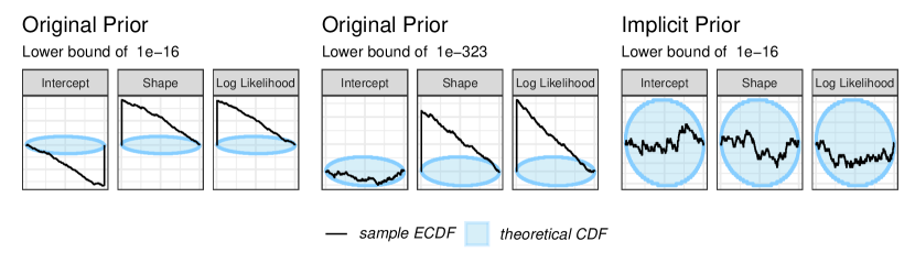
Figure 2: ECDF differences of exemplary selected variables for the model described in Equation (17). Generated SBC dateset outcomes were censored with a lower threshold of $1e-16$ (left and right) and $1e-323$ (middle). SBC with implicit priors used a preconditioning dataset of $N=15$. The plots using the original prior on the left and middle indicate severe calibration problems, while the plots using an implicit prior on the right indicates excellent calibration.

To better understand the scaling of the implicit prior with the size of the preconditioning dataset and the width of the original prior, as well as differences between preconditioning data-generating approaches, we ran a small simulation study. The different priors are based on the recommendations detailed in the Stan manual (Stan Development Team, 2023), namely a completely flat (improper) prior, a vague prior, a very weakly-informative prior, and a standard weakly-informative prior. The latter three are presented in Equations (18), (19), and (20), respectively. We selected several sample sizes for the preconditioning data from $N=5$ to $N=30$, with higher resolution around the number of model parameters (i.e., around $N=15$).

$$\begin{split}\beta_{0}&\sim\mathrm{Normal}(2,100)\\ \beta_{k}&\sim\mathrm{Normal}(0,100)\\ \alpha&\sim\mathrm{Gamma}(0.01,0.01)\end{split}$$ (18)

$$\begin{split}\beta_{0}&\sim\mathrm{Normal}(2,5)\\ \beta_{k}&\sim\mathrm{Normal}(0,1)\\ \alpha&\sim\mathrm{Gamma}(0.1,0.1)\end{split}$$ (19)

$$\begin{split}\beta_{0}&\sim\mathrm{Normal}(2,1)\\ \beta_{k}&\sim\mathrm{Normal}(0,1)\\ \alpha&\sim\mathrm{Gamma}(1,1)\end{split}$$ (20)

In addition to using subsets or power-scaled versions of the real bodyfat data for preconditioning, we also ran SBC using simulated preconditioning data, generated directly from the assumed gamma regression model. As fixed parameter values we chose, exemplarily, $\beta_{0}=1$, $\beta_{k}=0.1$ and $\alpha=1$. We repeated the simulations $T=10$ times, drawing a new preconditioning dataset for each run. We then drew $J=100$ SBC datasets $\tilde{y}^{(j)}$ with $50$ observations each per run, and drew $S=1000$ posterior samples per SBC model $M^{(t,j)}$ to calculate the rank statistic $R^{(t,j)}$.

The results are shown in Figure 3. Firstly, and of course unsurprisingly, we observe that more narrow priors result in better calibration across almost all cases (see below for the single exception). Similarly, larger preconditioning sample-sizes also result in better calibration. Around a sample size of $N=15$ (i.e., for $N$ equal to the number of model parameters), calibration starts to become adequate even for the flat and vague priors. Soon after (around $N=20$), calibration becomes almost perfect in all cases and stays perfect as $N$ further increases (not shown). The power-scaling based approach tends to reach calibration earlier than multiple subsetting and generally displays narrower intervals. This can be attributed to the higher variation in the outcomes when performing multiple subsetting due to the chance of drawing non-representative preconditioning datasets, whereas the power-scaling approach uses a larger (but downweighted) dataset for preconditioning. For a fixed preconditioning sample size, we also observe slightly better calibration when using simulated rather than real data for preconditioning. Apparently, the information gain from the simulated preconditioning data was higher than for the corresponding real data. Possible reasons include lower aleatoric uncertainty or smaller correlations between predictors in the simulated data for the chosen scenario. More generally, this highlights the source of preconditioning data as an important aspect when determining the required sample size.

The variation of calibration across parameters and preconditioning datasets was also larger in the real data preconditioning scenario, as can be seen from the size of the intervals displayed in Figure 3. This suggests a bigger variation across real data subsets compared to the variation across simulated datasets. Especially for smaller preconditioning sample sizes, results from individual preconditioning datasets might not be sufficiently reliable, which points to the importance of using several such preconditioning datasets rather than just a single one.

In terms of runtime, we found that the power-scaling (representative) priors lead to slightly slower model fitting times in cases of good calibration (35s compared to 30s for the multiple subsetting approach), but substantially slower in cases where calibration was not achieved (300s compared to 60s for the multiple subsetting approach). For this, we measured the runtime of drawing the SBC datasets $y_{j}$ and fitting the SBC models $M^{(j)}$, given a preconditioned model $M_{c}$. Based on the high number of SBC simulations $J$, this will represent the majority of the runtime in most cases. While the absolute runtimes for the procedure are specific to the present application and implementation, they show a tradeoff between the more robust results of using a power-scaling based priors and their somewhat higher computational demands. This is likely related to a more complex posterior geometry in the power-scaling case, which makes sampling more challenging.

Finally, we observed that the model with flat priors achieved better calibration than the model with vague priors, for any fixed preconditioning sample size, despite the flat priors being the actually wider ones. We assume that this specific issue is due to the choice of $\mathrm{Gamma}(0.01,0.01)$ prior for the shape parameter in the vague prior case, as it pushes a lot of prior-mass towards shapes of zero, thus making the likelihood very challenging numerically. Apparently, when aided by preconditioning, it is possible that improper priors imply better calibration more quickly compared to certain, even practically common, proper priors. In a different context, a similar phenomenon was described by Gelman (2006), where a very wide but simultaneously peaked inverse-gamma prior turned out to be much more informative than intended.

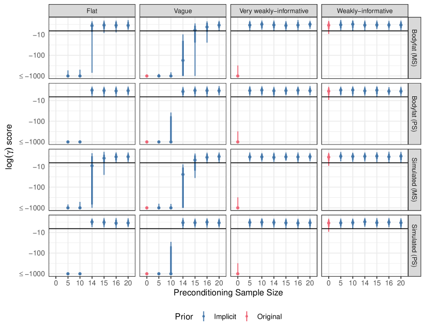
Figure 3: Scaling of the $\log(\gamma)$ score of the Gamma regression model described in Equation (17) for the different priors described in Equations (18), (19) and (20), different preconditioning dataset sources and sizes as well as both using a power-scaling (PS) and multiple subsetting (MS) approach for the implicit priors. Shown are the median as well as two-tailed 66% and 90% intervals of the $\log(\gamma)$ scores of all parameters across repetitions. The horizontal line indicates the threshold to reject uniformity at a nominal Type 1 error rate of 5% to match the two-tailed 90% interval. Generated SBC dateset outcomes were censored with a lower threshold of $1e-16$. Traditional SBC is generally not computable for a flat (improper) prior.

In summary, we found that implicit priors based on both real and simulated data help in stabilizing SBC for the shown gamma regression. The minimally required preconditioning sample size to achieve sufficient calibration depends on the chosen prior and the data source. That said, using a preconditioning sample size equal to the number of model parameters appears to be a good starting point, at least for simple models and when working with vague or flat priors.

4.2 Implicit priors for latent variable models

As models become more complex, the resulting posterior may present a challenge for effective exploration via MCMC methods. This means that even when the model is correctly implemented and the desired prior distribution can be used as-is for data generation (i.e. without any rejection sampling), SBC can still fail. In this case study, we demonstrate such an issue with one model that we built to test a framework for estimation of heteroscedastic latent variables Fazio and Bürkner (2024).

Specifically, the model represents a mediation analysis, where the effects that one variable has on the mean and standard deviation of another variable are hypothesized to be potentially explained by changes in intervening variables. We provide a graphical representation of the model in Figure 4 and explain the mathematical details below. Let us use $\zeta_{li}$ to represent the $i$-th realization of the $l$-th latent variable, with associated parameters $\mu_{li}$ and $\sigma_{li}$. When these parameters are fixed, the second index is omitted. Otherwise, there is an associated linear predictor, with coefficients $\beta_{k\theta_{l}}$ denoting the slope for the $k$-th predictor of the parameter $\theta$ (i.e., $\mu$ or $\sigma$) associated with the $l$-th latent variable. The mathematical notation for the latent structural model is

$$\begin{split}\zeta_{1i}&\sim\text{Normal}(0,\sigma_{1})\\ \zeta_{2i}&\sim\text{Normal}(\mu_{2i},\sigma_{2})\\ \mu_{2i}&=\beta_{1\mu_{2}}\zeta_{1}\\ \zeta_{3}&\sim\text{Normal}(\mu_{3},\sigma_{3})\\ \mu_{3}&=\beta_{1\mu_{3}}\zeta_{1}\\ \zeta_{4}&\sim\text{Normal}(\mu_{4},\sigma_{4})\\ \mu_{4}&=\beta_{1\mu_{4}}\zeta_{1}+\beta_{2\mu_{4}}\zeta_{2}\\ \log\sigma_{4}&=\beta_{0\sigma_{4}}+\beta_{1\sigma_{4}}\zeta_{1}+\beta_{2\sigma_{4}}\zeta_{3}.\end{split}$$ (21)

We use a Gaussian measurement model, such that the $j$-th indicator variable $y_{jli}$ is related to the $i$-th realization of the $l$-th latent variable through a slope $\lambda_{jl}$ (sometimes called factor loading) and an intercept $\nu_{jl}$. The standard deviation of the measurement error is $\tau_{jl}$. The corresponding notation is

$$\begin{split}y_{jli}&\sim\text{Normal}(\nu_{jl}+\lambda_{jl}\,\zeta_{li},\tau_{jl}).\end{split}$$ (22)

For this simulation, we use $j\in\{1,2,3\}$ indicator variables, $l\in\{1,2,3,4\}$ latent variables, and $i\in\{1,\dots,75\}$ observations per variable.

Figure 4: Graphical representation of the relationship between the latent variables in our mediation model. $\zeta_{1}$ has direct and indirect effects on both of $\zeta_{4}$’s mean and standard deviation parameters through $\zeta_{2}$ and $\zeta_{3}$, respectively. These variables are latent and so are only indirectly observed through the measurement model described in Equation 22.

Table 1: Prior specification for the latent variable model.

Parameter type	Notation	Weakly informative prior	Fixed generative parameters
Latent mean
Slope	$\beta_{\mu}$	Normal(0, 10)	0
Latent std. dev.
Fixed	$\sigma$	$\text{Gamma}(1,0.5)$	1
Intercept	$\beta_{0\sigma}$	$\text{Exp-Gamma}(1,0.5)$	0
Slope	$\beta_{\geq 1\sigma}$	$\text{Normal}(0,\,2.5)$	0
Indicator parameters
Factor loading	$\lambda$	$\text{Normal}(0,\,10)$	1
Intercept	$\nu$	$\text{Normal}(0,\,32)$	0
Error std. dev.	$\tau$	Gamma(1, 0.5)	1

Now, consider the first set of priors shown in Table 1. These are based on the defaults used by blavaan, a package for Bayesian latent variable models (Merkle et al., 2021). Taken separately, each of the priors constitutes a reasonable weakly informative choice for its corresponding parameter. However, if one examines the implied prior predictive distribution for $\zeta_{4}$, it turns out to vary over a range that is orders of magnitude larger than those of the preceding variables (Table 2).

Table 2: Empirical prior predictive distribution of the latent variables using the weakly informative prior. Samples were pooled across the 200 datasets generated by drawing parameters from the prior, each with $N=75$.

	Quantiles
Variable	10%	25%	50%	75%	90%
$\zeta_{1}$	-2.8	-0.8	0	0.8	2.6
$\zeta_{2},\zeta_{3}$	-18.1	-5.2	0	5.2	18.7
$\zeta_{4}$	$-9.0\times 10^{9}$	-178	-1.4	143	$3.2\times 10^{10}$

This prior specification is already unsatisfactory because it does a poor job of encoding what we believe a reasonable data-generating process would look like, but a bigger problem is that it interacts with the model likelihood to produce a posterior which Stan’s MCMC sampler badly fails at recovering. The key challenge is that information about latent variances is only available in the data as a component of the total variance of the indicator variables, which also includes the error variances ($\tau$):

$$\begin{split}\text{Var}(y_{jli})=\lambda^{2}_{jl}\text{Var}(\zeta_{li})+\tau_{jl}.\end{split}$$ (23)

The equation above shows that there has to be a direct trade-off between the magnitudes these variances can take. Furthermore, the weakly informative prior implies a high prior probability of both $\sigma_{4}$ having near-zero values, and of $\sigma_{4}<\tau_{j4}$. As a result, the sampler will be stuck in the mode that assigns most of the observed variance to the $\tau_{j4}$ parameters, leading to vastly overestimated $\tau_{j4}$ values and underestimated $\sigma_{4}$ values (see Table 3).

Table 3: We sample from the respective pushforward distributions to recover the implied prior on $\sigma_{4}$ (first row) and see that, given the Gamma$(1,0.5)$ prior on $\tau_{j4}$ (second row), this implies $P(\sigma_{4}<\tau_{j4})>0.5$. The SBC posterior (third row) should recover the prior for $\tau_{j4}$ but instead the sampler favors far larger estimates (convergence also fails badly, so the exact values are not meaningful).

	Quantiles
Distribution	10%	25%	50%	75%	90%
Implied $p(\sigma_{4})$	$1.8\times 10^{-5}$	$1.8\times 10^{-2}$	1.2	67	$7.5\times 10^{4}$
$p(\tau_{j4})$	0.2	0.6	1.4	2.8	4.6
$p_{\text{SBC}}(\tau_{j4}\mid y)$	113	$2.3\times 10^{7}$	$2.7\times 10^{17}$	$8.2\times 10^{40}$	$1.6\times 10^{63}$

Attempting to perform SBC with such a prior will readily reveal that the resulting posterior approximations are grossly miscalibrated. Rejection sampling will not help here: across all of the simulated datasets, there was not a single converging fit, with Stan’s MCMC sampler failing to even initialize in some cases. This is a scenario where we must accept the gap between the models we can define mathematically and those that we can fit in practice. Fortunately, we have already established that such a weakly informative prior includes parameter combinations that are not of interest to us, so we could try finding a different prior to produce posteriors that are easier to sample from. Reducing the scale of the original priors may seem like a straightforward way of achieving this, but striking the right balance between informativeness and stability would require one to conduct a tedious iterative process for each set of parameters. By contrast, the implicit prior approach just requires us to specify a single point in parameter space that we can simulate reasonable data from. From there, one can continue to iterate over the size of the preconditioning sample until the desired criteria are satisfied.

The fixed set of parameter values we used in this case study is listed in the last column of Table 1. Following the notation in Section 3.6, we drew $J=200$ SBC datasets $\tilde{y}^{(j)}$, each with $75$ observations and a total of $T=40$ preconditioning datasets.

When constructing the preconditioning datasets for this model, we opted to leave in the "true" generated latent variables, i.e. treat them as observed (as discussed in Section 3.7). This was necessary in order to provide information on the latent scales while keeping the number of preconditioning observations small. Although this may intuitively cause concerns regarding the effect on latent variables that will be estimated from the actual data, it must be considered that the latent variables at each observation are separate parameters. Therefore, the model can be regarded as being already factorized in a way that prevents these imaginary observations from directly affecting the estimation of the remaining latent variables. This can be considered as an instance where informing only a subset of model parameters is both desirable and easily implemented.

Our results show that the issues with model miscalibration and non-convergence are promptly resolved with implicit priors, even for a preconditioning sample of just $N=10$ (Figure 5). This matches the number of global parameters that characterize the latent variables and the relationships between them, once again matching the heuristic discussed in Section 3.4.

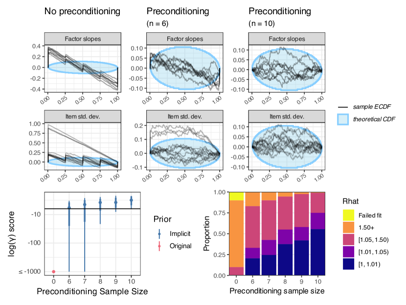
Figure 5: Top: ECDF difference plots for selected parameters. The weakly informative prior clearly leads to a miscalibrated posterior. The three tall peaks in the first $\tau$ panel reflect extreme miscalibration of the three $\tau_{j4}$, but we can see problems there propagate to other parameters in the model, including slopes, which are usually of central interest. Notice that the sawtooth pattern with four segments matches the four chains used per fit, which indicates that most fits had a stuck sampler. Bottom left: Plotting the log-gamma statistics for all model parameters allow us to visualize the global improvement in calibration with increasing size of the preconditioning dataset. Bottom right: Convergence also improves with preconditioning.

5 Conclusion

This paper is concerned with obtaining implicit priors from various data sources, including both real and simulated data, as well as their practical use with probabilistic programming languages. We placed specific focus on Bayesian generative modeling and simulation studies, in particular simulation-based calibration (SBC) to verify the correctness of probabilistic inference. The results obtained in our case studies confirm that implicit priors, preconditioned on only a little data, quickly lead to more realistic (less extreme) simulation outcomes and stable SBC results. Depending on the type of implicit prior and source of the preconditioning data, the minimal number of preconditioning observations yielding stable simulations varied slightly but was rarely much larger than the number of (top-level) model parameters; even for completely flat base priors. Except for data-sparse scenarios, such sizes of preconditioning data will usually be small in comparison to the size of the actual datasets being analysed by means of the Bayesian models under scrutiny. Thus, using implicit priors in a Bayesian simulation workflow will usually cause only little computational overhead. In summary, implicit priors can offer substantial benefits for practitioners in scenarios that heavily depend on prior choice while simultaneously lacking sufficiently informative priors at hand. In particular, this simplifies setting up realistic and stable Bayesian simulation studies.

We have mainly focused on SBC as a prominent case of Bayesian simulations, but other types of simulation studies may also benefit from implicit priors. For example, creating comparable ground-truths across different data-generating processes can be exceedingly difficult, since prior hyperparameters are hard to match across non-nested model classes (Scholz and Bürkner, 2023a, b). By using the same preconditioning data to create implicit priors for all models, the resulting (distribution of) ground truths should become more comparable. The remaining differences are then more likely to be caused by the structural model differences of interest and less so by artifacts created through incomparable choices of prior hyperparameters. Implicit priors may also be useful to achieve fairer comparisons of inference algorithms. For example, when comparing asymptotically unbiased algorithms such as MCMC, with (potentially) asymptotically biased algorithms such as black-box variational inference (Ranganath et al., 2014), Laplace approximation (Rue et al., 2017), or pathfinder (Zhang et al., 2022), the results are likely strongly dependent on the underlying true data-generating process. By obtaining more realistic data-generating processes through implicit priors, it should be possible to draw more reliable conclusions about the algorithms’ real-world differences.

Statements and Declarations

This work was partially funded by the Deutsche Forschungsgemeinschaft (DFG, German Research Foundation) under Germany’s Excellence Strategy – EXC-2075 - 390740016 (the Stuttgart Cluster of Excellence SimTech) and DFG project grant 497785967. The authors gratefully acknowledge the support and funding.

The authors would like to thank Javier Enrique Aguilar for his thoughtful comments and discussion on earlier versions of the manuscript

The authors have no competing interests to declare that are relevant to the content of this article.

Data and code availability

The data and code that support the findings of this study are openly available in OSF at https://osf.io/ad7qu/.

References

- Anscombe and Tukey [1963] Francis J. Anscombe and John W. Tukey. The examination and analysis of residuals. Technometrics, 5(2):141–160, 1963.
- D’Agostino [1986] Ralph B. D’Agostino. Goodness-of-Fit Techniques. Routledge, 1 edition, 1986. doi:10.1201/9780203753064.
- Gelman et al. [1996] Andrew Gelman, Xiao-Li Meng, and Hal Stern. Posterior predictive assessment of model fitness via realized discrepancies. Statistica sinica, pages 733–760, 1996.
- Gelman et al. [2020] Andrew Gelman, Aki Vehtari, Daniel Simpson, Charles C Margossian, Bob Carpenter, Yuling Yao, Lauren Kennedy, Jonah Gabry, Paul-Christian Bürkner, and Martin Modrák. Bayesian workflow. arXiv preprint, 2020. doi:10.48550/arXiv.2011.01808.
- Gabry et al. [2019] Jonah Gabry, Daniel Simpson, Aki Vehtari, Michael Betancourt, and Andrew Gelman. Visualization in Bayesian workflow. Journal of the Royal Statistical Society: Series A (Statistics in Society), 2019. doi:10.1111/rssa.12378.
- Gelman et al. [2017] Andrew Gelman, Daniel Simpson, and Michael Betancourt. The prior can often only be understood in the context of the likelihood. Entropy, 19(10):555–567, 2017. doi:10.3390/e19100555.
- Mikkola et al. [2023] Petrus Mikkola, Osvaldo A. Martin, Suyog Chandramouli, Marcelo Hartmann, Oriol Abril Pla, Owen Thomas, Henri Pesonen, Jukka Corander, Aki Vehtari, Samuel Kaski, Paul-Christian Bürkner, and Arto Klami. Prior Knowledge Elicitation: The Past, Present, and Future. Bayesian Analysis, 2023. doi:10.1214/23-BA1381.
- Aguilar and Bürkner [2023] Javier Enrique Aguilar and Paul-Christian Bürkner. Intuitive joint priors for Bayesian linear multilevel models: The R2D2M2 prior. Electronic Journal of Statistics, 2023. doi:10.1214/23-EJS2136.
- Talts et al. [2020] Sean Talts, Michael Betancourt, Daniel Simpson, Aki Vehtari, and Andrew Gelman. Validating Bayesian Inference Algorithms with Simulation-Based Calibration. arXiv preprint, 2020. doi:10.48550/arXiv.1804.06788.
- Modrák et al. [2023] Martin Modrák, Angie H. Moon, Shinyoung Kim, Paul Bürkner, Niko Huurre, Kateřina Faltejsková, Andrew Gelman, and Aki Vehtari. Simulation-Based Calibration Checking for Bayesian Computation: The Choice of Test Quantities Shapes Sensitivity. Bayesian Analysis, 2023. doi:10.1214/23-BA1404.
- Good [1950] Isidore J. Good. Probability and the Weighing of Evidence. Charles Griffin & Company Limited: London, 1950.
- Winkler [1967] Robert L. Winkler. The assessment of prior distributions in bayesian analysis. Journal of the American Statistical Association, 62(319):776–800, 1967.
- Zellner [1986] Arnold Zellner. On assessing prior distributions and Bayesian regression analysis with g-prior distributions. Bayesian inference and decision techniques, 1986.
- Maruyama and George [2011] Yuzo Maruyama and Edward I. George. Fully Bayes factors with a generalized g-prior. The Annals of Statistics, 39(5), October 2011. doi:10.1214/11-AOS917.
- Sabanés Bové and Held [2011] Daniel Sabanés Bové and Leonhard Held. Hyper- priors for generalized linear models. Bayesian Analysis, 6(3), September 2011. doi:10.1214/11-BA615.
- Chen et al. [1998] Ming-Hui Chen, Amita K. Manatunga, and Christopher J. Williams. Heritability Estimates from Human Twin Data by Incorporating Historical Prior Information. Biometrics, 54(4):1348, December 1998. doi:10.2307/2533662.
- Ibrahim and Chen [2000] Joseph G. Ibrahim and Ming-Hui Chen. Power Prior Distributions for Regression Models. Statistical Science, 2000.
- Chen and Ibrahim [2003] Ming-Hui Chen and Joseph G Ibrahim. Conjugate priors for generalized linear models. Statistica Sinica, pages 461–476, 2003.
- Kallioinen et al. [2024] Noa Kallioinen, Topi Paananen, Paul-Christian Bürkner, and Aki Vehtari. Detecting and diagnosing prior and likelihood sensitivity with power-scaling. Statistics and Computing, 34(1):57, 2024.
- Ibrahim et al. [2015] Joseph G. Ibrahim, Ming-Hui Chen, Yeongjin Gwon, and Fang Chen. The power prior: Theory and applications. Statistics in Medicine, 2015. doi:10.1002/sim.6728.
- Perez and Berger [2002] José M. Perez and James O. Berger. Expected-posterior prior distributions for model selection. Biometrika, 89(3):491–512, August 2002. doi:10.1093/biomet/89.3.491.
- Fouskakis et al. [2015] Dimitris Fouskakis, Ioannis Ntzoufras, and David Draper. Power-Expected-Posterior Priors for Variable Selection in Gaussian Linear Models. Bayesian Analysis, 10(1), March 2015. doi:10.1214/14-BA887.
- Fouskakis [2019] D. Fouskakis. Priors via imaginary training samples of sufficient statistics for objective Bayesian hypothesis testing. METRON, 77(3):179–199, December 2019. doi:10.1007/s40300-019-00159-0.
- Tzoumerkas et al. [2022] G. Tzoumerkas, D. Fouskakis, and I. Ntzoufras. A Comparison of Power–Expected–Posterior Priors in Shrinkage Regression. Journal of Statistical Theory and Practice, 16(4):61, December 2022. doi:10.1007/s42519-022-00284-6.
- Aitkin [1991] Murray Aitkin. Posterior Bayes Factors. Journal of the Royal Statistical Society Series B: Statistical Methodology, 53(1):111–128, September 1991. doi:10.1111/j.2517-6161.1991.tb01812.x.
- O’Hagan [1995] Anthony O’Hagan. Fractional Bayes Factors for Model Comparison. Journal of the Royal Statistical Society: Series B (Methodological), 1995. doi:10.1111/j.2517-6161.1995.tb02017.x.
- Gu et al. [2018] Xin Gu, Joris Mulder, and Herbert Hoijtink. Approximated adjusted fractional Bayes factors: A general method for testing informative hypotheses. British Journal of Mathematical and Statistical Psychology, 71(2):229–261, May 2018. doi:10.1111/bmsp.12110.
- Berger and Pericchi [1996] James O. Berger and Luis R. Pericchi. The Intrinsic Bayes Factor for Model Selection and Prediction. Journal of the American Statistical Association, 1996. doi:10.1080/01621459.1996.10476668.
- Moreno and Pericchi [2014] Elías Moreno and Luís Raúl Pericchi. Intrinsic Priors for Objective Bayesian Model Selection. In Bayesian Model Comparison, Advances in Econometrics. Emerald Group Publishing Limited, 2014. doi:10.1108/S0731-905320140000034012.
- Stan Development Team [2024a] Stan Development Team. Stan Modeling Language Users Guide and Reference Manual, 2.34, 2024a.
- Abril-Pla et al. [2023] Oriol Abril-Pla, Virgile Andreani, Colin Carroll, Larry Dong, Christopher J Fonnesbeck, Maxim Kochurov, Ravin Kumar, Junpeng Lao, Christian C Luhmann, Osvaldo A Martin, et al. Pymc: a modern, and comprehensive probabilistic programming framework in python. PeerJ Computer Science, 9:e1516, 2023.
- Ge et al. [2018] Hong Ge, Kai Xu, and Zoubin Ghahramani. Turing: a language for flexible probabilistic inference. In International Conference on Artificial Intelligence and Statistics, AISTATS 2018, 9-11 April 2018, Playa Blanca, Lanzarote, Canary Islands, Spain, pages 1682–1690, 2018. URL http://proceedings.mlr.press/v84/ge18b.html.
- Bhattacharya et al. [2019] Anirban Bhattacharya, Debdeep Pati, and Yun Yang. Bayesian fractional posteriors. The Annals of Statistics, 2019. doi:10.1214/18-AOS1712.
- Bardenet et al. [2017] Rémi Bardenet, Arnaud Doucet, and Chris Holmes. On markov chain monte carlo methods for tall data. Journal of Machine Learning Research, 18(47):1–43, 2017.
- Schmidli et al. [2014] Heinz Schmidli, Sandro Gsteiger, Satrajit Roychoudhury, Anthony O’Hagan, David Spiegelhalter, and Beat Neuenschwander. Robust Meta-Analytic-Predictive Priors in Clinical Trials with Historical Control Information. Biometrics. Journal of the International Biometric Society, 2014. doi:10.1111/biom.12242.
- Hall et al. [2021] Kathryn T. Hall, Lene Vase, Deirdre K. Tobias, Hesam T. Dashti, Jan Vollert, Ted J. Kaptchuk, and Nancy R. Cook. Historical Controls in Randomized Clinical Trials: Opportunities and Challenges. Clinical Pharmacology & Therapeutics, 2021. doi:10.1002/cpt.1970.
- Ren et al. [2010] Shiquan Ren, Hong Lai, Wenjing Tong, Mostafa Aminzadeh, Xuezhang Hou, and Shenghan Lai. Nonparametric bootstrapping for hierarchical data. Journal of Applied Statistics, 2010. doi:10.1080/02664760903046102.
- Simpson et al. [2017] Daniel Simpson, Håvard Rue, Andrea Riebler, Thiago G Martins, and Sigrunn H Sørbye. Penalising model component complexity: A principled, practical approach to constructing priors. Statistical science, 2017. doi:10.1214/16-STS576.
- Alizadeh et al. [2020] Reza Alizadeh, Janet K. Allen, and Farrokh Mistree. Managing computational complexity using surrogate models: A critical review. Research in Engineering Design, 2020. doi:10.1007/s00163-020-00336-7.
- Cranmer et al. [2020] Kyle Cranmer, Johann Brehmer, and Gilles Louppe. The frontier of simulation-based inference. Proceedings of the National Academy of Sciences, 2020. doi:10.1073/pnas.1912789117.
- Bürkner et al. [2023] Paul-Christian Bürkner, Maximilian Scholz, and Stefan T. Radev. Some models are useful, but how do we know which ones? Towards a unified Bayesian model taxonomy. Statistics Surveys, 2023. doi:10.1214/23-SS145.
- Gelman et al. [2013] Andrew Gelman, John B Carlin, Hal S Stern, David B Dunson, Aki Vehtari, and Donald B Rubin. Bayesian Data Analysis (3rd Edition). London: Chapman and Hall/CRC, 2013.
- Säilynoja et al. [2022] Teemu Säilynoja, Paul-Christian Bürkner, and Aki Vehtari. Graphical test for discrete uniformity and its applications in goodness-of-fit evaluation and multiple sample comparison. Statistics and Computing, 2022. doi:10.1007/s11222-022-10090-6.
- R Core Team [2024] R Core Team. R: A Language and Environment for Statistical Computing. Vienna, Austria, 2024.
- Stan Development Team [2024b] Stan Development Team. RStan: The R interface to Stan, 2024b.
- Gabry et al. [2024] Jonah Gabry, Rok Češnovar, and Andrew Johnson. cmdstanr: R interface to ’cmdstan’, 2024. URL https://github.com/stan-dev/cmdstanr.
- Bürkner [2017] Paul-Christian Bürkner. Brms: An R package for Bayesian multilevel models using Stan. Journal of statistical software, 2017. doi:10.18637/jss.v080.i01.
- Wickham et al. [2019] Hadley Wickham, Mara Averick, Jennifer Bryan, Winston Chang, Lucy D’Agostino McGowan, Romain François, Garrett Grolemund, Alex Hayes, Lionel Henry, Jim Hester, Max Kuhn, Thomas Lin Pedersen, Evan Miller, Stephan Milton Bache, Kirill Müller, Jeroen Ooms, David Robinson, Dana Paige Seidel, Vitalie Spinu, Kohske Takahashi, Davis Vaughan, Claus Wilke, Kara Woo, and Hiroaki Yutani. Welcome to the tidyverse. Journal of Open Source Software, 2019. doi:10.21105/joss.01686.
- Scholz and Bürkner [2024] Maximilian Scholz and Paul-Christian Bürkner. Bayesim, August 2024. URL https://doi.org/10.5281/zenodo.13284425.
- Landau [2021] William Michael Landau. The targets r package: a dynamic make-like function-oriented pipeline toolkit for reproducibility and high-performance computing. Journal of Open Source Software, 6(57):2959, 2021. URL https://doi.org/10.21105/joss.02959.
- Fazio et al. [2024] Luna Fazio, Maximilian Scholz, and Paul-Christian Bürkner. Online appendix for Generative Bayesian Modeling with Implicit Priors manuscript, August 2024. URL https://doi.org/10.5281/zenodo.13284509.
- Johnson [1996] Roger W. Johnson. Fitting Percentage of Body Fat to Simple Body Measurements. Journal of Statistics Education, 1996. doi:10.1080/10691898.1996.11910505.
- Stan Development Team [2023] Stan Development Team. Prior Choice Recommendations, 2023. URL https://github.com/stan-dev/stan/wiki/Prior-Choice-Recommendations.
- Modrák [2024] Martin Modrák. Rejection sampling in simulations, 2024. URL https://hyunjimoon.github.io/SBC/articles/rejection_sampling.html.
- Gelman [2006] Andrew Gelman. Prior distributions for variance parameters in hierarchical models (comment on article by Browne and Draper). Bayesian Analysis, 2006. doi:10.1214/06-BA117A.
- Fazio and Bürkner [2024] Luna Fazio and Paul-Christian Bürkner. Gaussian distributional structural equation models: A framework for modeling latent heteroscedasticity. arXiv preprint, 2024. doi:10.48550/arXiv.2404.14124.
- Merkle et al. [2021] Edgar C. Merkle, Ellen Fitzsimmons, James Uanhoro, and Ben Goodrich. Efficient Bayesian Structural Equation Modeling in Stan. Journal of Statistical Software, 100(6), 2021. doi:10.18637/jss.v100.i06.
- Scholz and Bürkner [2023a] Maximilian Scholz and Paul-Christian Bürkner. Prediction can be safely used as a proxy for explanation in causally consistent Bayesian generalized linear models. arXiv preprint, 2023a. doi:10.48550/arXiv.2210.06927.
- Scholz and Bürkner [2023b] Maximilian Scholz and Paul-Christian Bürkner. Posterior accuracy and calibration under misspecification in Bayesian generalized linear models. arXiv preprint, 2023b. doi:10.48550/arXiv.2311.09081.
- Ranganath et al. [2014] Rajesh Ranganath, Sean Gerrish, and David Blei. Black Box Variational Inference. In Proceedings of the Seventeenth International Conference on Artificial Intelligence and Statistics. PMLR, 2014.
- Rue et al. [2017] Håvard Rue, Andrea Riebler, Sigrunn H Sørbye, Janine B Illian, Daniel P Simpson, and Finn K Lindgren. Bayesian computing with INLA: A review. Annual Review of Statistics and Its Application, 2017.
- Zhang et al. [2022] Lu Zhang, Bob Carpenter, Andrew Gelman, and Aki Vehtari. Pathfinder: Parallel quasi-Newton variational inference. Journal of Machine Learning Research, 2022.