Radiative corrections relating leptoquark-fermion couplings probed at low and high energy

Abstract

Scalar leptoquarks (LQ) with masses between 2 TeV and 50 TeV are prime candidates to explain deviations between measurements and Standard-Model predictions in decay observables of $b$-flavored hadrons (“flavor anomalies”). Explanations of low-energy data often involve ${\cal O}(1)$ LQ-quark-lepton Yukawa couplings, especially when collider bounds enforce a large LQ mass. This calls for the calculation of radiative corrections involving these couplings. Studying such corrections to LQ-mediated $b\to c\tau\nu$ and $b\to s\ell^{+}\ell^{-}$ amplitudes, we find that they can be absorbed into finite renormalizations of the LQ Yukawa couplings. If one wants to use Yukawa couplings extracted from low-energy data for the prediction of on-shell LQ decay rates, one must convert the low-energy couplings to their high-energy counterparts, which subsume the corrections to the on-shell LQ-quark-lepton vertex. We present compact formulae for these correction factors and find that in scenarios with $S_{1}$, $R_{2}$, or $S_{3}$ LQ the high-energy coupling is always smaller than the low-energy one, which weakens the impact of collider data on the determination of the allowed parameter spaces. For the $R_{2}$ scenario addressing $b\to c\tau\nu$, in which one of the two involved Yukawa coupling must be significantly larger than 1, we find this coupling reduced by 15% at high energy. If both $S_{1}$ and $R_{2}$ are present, the high-energy coupling can also be larger and the size of the correction is unbounded, because tree contribution and vertex corrections involve different couplings. We further present the conversion formula to the $\overline{\rm MS}$ scheme for the Yukawa couplings of the $S_{3}$ scenario.

1 Introduction

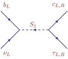
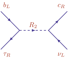
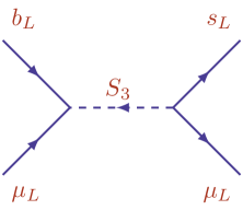
Figure 1: Contributions of scalar leptoquarks to the decay modes $b\to c\tau^{-}\bar{\nu}$ and $b\to s\mu^{+}\mu^{-}$.

 

Leptoquarks (LQs) are hypothetical particles that directly couple to Standard Model (SM) leptons and quarks. They feature in many models for Beyond the Standard Model (BSM) physics and, in particular, TeV-scale leptoquarks remain phenomenologically well-motivated candidates (see e.g. Refs. Raj:2016aky ; Diaz:2017lit ; Bansal:2018eha ; Schmaltz:2018nls ; Bhaskar:2021gsy ; Bernigaud:2021fwn ; Dorsner:2022ibm ; Goncalves:2023qpz ; Bhaskar:2023ftn ) for searches at the Large Hadron Collider driven by the quark transitions $b\to s\ell^{+}\ell^{-}$, where $\ell=e,\mu$, LHCb:2015ycz ; LHCb:2015wdu ; ATLAS:2018cur ; CMS:2018qih ; LHCb:2018jna ; CMS:2019bbr ; BELLE:2019xld ; CMS:2020oqb ; LHCb:2020dof ; LHCb:2020gog ; LHCb:2021vsc ; LHCb:2021trn ; LHCb:2021xxq ; LHCb:2021lvy ; LHCb:2021zwz ; LHCb:2022qnv ; LHCb:2022zom and $b\to c\tau\nu$ HFLAV:2022esi deviate from their Standard-Model (SM) predictions. To date, scalar leptoquarks (LQs) are the most popular particle species postulated to remedy these flavor anomalies (see e.g. Refs. Sakaki:2013bfa ; Dorsner:2016wpm ; Dumont:2016xpj ; Li:2016vvp ; Bhattacharya:2016mcc ; Chen:2017hir ; Crivellin:2017zlb ; Cai:2017wry ; Jung:2018lfu ; Aydemir:2019ynb ; Popov:2019tyc ; Crivellin:2019dwb ; Bigaran:2019bqv ; Bansal:2018nwp ; Iguro:2020keo ; Ciuchini:2022wbq ). Fig. 1 illustrates the contributions of the scalar leptoquarks $S_{1}\sim(\bar{3},1,1/3)$, $R_{2}\sim(3,2,7/6)$, and $S_{3}~{}\sim(\bar{3},3,1/3)$ to the quark decay amplitudes of interest. Additionally, for example, both $S_{1}$ and $R_{2}$ are capable of generating large chirally-enhanced contributions to the muon and electron anomalous magnetic moments (see e.g. Ref. Bigaran:2020jil ), and all three leptoquarks may play a role in models for radiative neutrino mass generation (see e.g. Ref. Gargalionis:2020xvt ).

Typically, low-energy physics observables enable the determination of the ratio between the product of the couplings involved and the square of the LQ mass. This, in conjunction with current constraints on LQ searches, defines a target parameter space to be explored at high-energy colliders. To avoid present collider search bounds, LQ masses should exceed approximately 2 TeV (see e.g. Refs. CMS:2018qqq ; ATLAS:2019qpq ). Consequently, a model incorporating LQs such as $S_{1}$ or $R_{2}$ to explain the $b\to c\tau\nu$ data must possess $\mathcal{O}(1)$ LQ-quark-lepton couplings to generate a sufficiently large effect. For $S_{3}$, there is more flexibility – $\mathcal{O}(1)$ couplings are only necessary for a LQ mass around 30 TeV Fedele:2023rxb , a value far from being reached at the LHC. Therefore, at least for $S_{1}$ and $R_{2}$ significant radiative corrections are expected from loops involving these couplings, implying that the couplings affecting low-energy data may significantly differ numerically from those influencing high-energy phenomenology.

Moreover, any particular model built for a given phenomenological purpose may contain multiple leptoquarks. For example they may come in several copies, e.g. at least two copies are needed for $S_{3}$ to address $b\to s\ell\ell$ data: $S_{3\,{e}}$ couples to $e$ but not to $\mu$ while for $S_{3\,{\mu}}$ the situation is opposite. Therefore, the interplay between the presence of multiple LQs for such aforementioned radiative corrections could provide new ways to indirectly search for evidence of multi-particlular models.

Direct searches for new heavy particles at the LHC have thus far yielded no success, indicating a significant gap between the electroweak (EW) scale and the scale of BSM physics. Previous investigations into LQs in low-energy observables have incorporated QCD radiative corrections in the conventional manner, by matching the LQ-mediated amplitudes to the weak effective theory (WET) and employing renormalization group equations (RGEs) to evolve the resulting Wilson coefficients (WCs) from the renormalization scale $\mu_{\text{high}}\sim M_{\text{LQ}}$ (denoting the mass of the relevant LQ) to $\mu_{\text{low}}\sim m_{b}$, relevant to the $b$-flavored hadron decays of interest. This procedure effectively sums large logarithms multiplied by the strong coupling $\alpha_{s}$. The focus of this paper, however, are genuine additional correction factors involving LQ couplings rather than $\alpha_{s}$, and solely enter the WCs at $\mu_{\rm high}$. In this way, these corrections modify the initial conditions for the WCs and the corrected coefficients can simply be evolved to $\mu_{\rm low}$ with the standard leading-log RGEs.

When solely performing calculations of high-scale quantities, such as LQ production cross sections and LQ decay rates, all couplings come into play at the renormalization scale $\mu_{\text{high}}$, and no RGE running or matching procedure is required. Radiative one-loop corrections involving LQ-fermion couplings do not involve large logarithms, and in both high-energy and low-energy observables, these couplings are typically probed at the renormalization scale $\mu_{\text{high}}$. An important distinction between collider and flavor physics observables is the relevant momenta $p_{i}^{{\mu}}$ entering the loop diagrams: in collider observables, $|p_{i}^{{\mu}}|\approx M_{\text{LQ}}$, whereas in $b$ decays, $|p_{i}^{{\mu}}|\approx m_{b}\approx 0$. When we refer to “energy” in this paper, we are referring to the magnitude of these momenta $p_{i}^{{\mu}}$, i.e., the energy scale at which the LQ interaction is probed, and not the renormalization scale $\mu$.

If one determines the low-energy LQ-fermion couplings from flavor observables, they can use the results of this paper to calculate the corresponding couplings at high energies. The tree amplitude then expressed in terms of these high-energy couplings contains the one-loop corrections to the LQ decay rate exactly. If one next wants to predict the corrections to the LQ production cross section at the LHC (or another high-energy collider), there will be additional loop diagrams to consider, which are, however, specific to the considered production process.

For instance, a quark-gluon initiated process involves diagrams with off-shell LQ or fermion lines at the production vertex, each coming with different kinematics and, furthermore, a gluon-LQ-LQ vertex. The process-dependent corrections can be consistently calculated in the renormalization scheme in which the LQ-quark-lepton coupling is defined at the high-energy scale, which breaks the radiative corrections up into a piece contained in our calculation and the process-specific remainder. Thus our corrections do not fully subsume all radiative corrections to LQ production.

The corrections calculated in this work are universal, renormalization-scheme independent, and capture all effects related to the LQ decay vertex. These may therefore be easily included in simulations with tree-level event generators.

In Section 2 we explain our approach by providing a definition of couplings at low and high energies, then proceed with the calculation of corrections. Section 3 is devoted to a discussion of the phenomenological consequences of these results. We summarise our introduced formalism and conclude in Section 4.

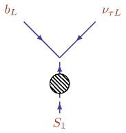
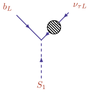
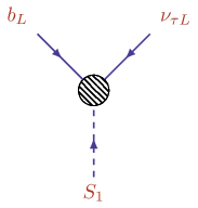
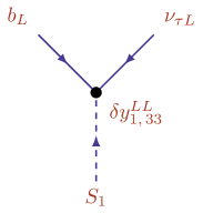
Figure 2: Radiative corrections to the $S_{1}$-$b_{L}$-$\nu_{\tau L}$ vertex ($y_{1\,33}^{LL}$). The final diagram depicts the contribution from the coupling counterterm, $\delta y_{1\,33}^{LL}$.

 

2 Calculation

The relevant Yukawa couplings of the LQ Lagrangian are given by

$$\mathcal{L}_{\rm LQ} = {\sum_{j,k=1}^{3}\sum_{a,b=1}^{2}}\Big{[}y_{1\,jk}^{LL}\,\overline{Q^{c}_{L}}{}^{j,a}\,\epsilon^{ab}L_{L}^{k,b}\,S_{1}\;+\;y_{1\,jk}^{RR}\,\overline{u_{R}^{c}}{}^{j}e_{R}^{k}\,S_{1}$$ (1)

$$\phantom{\sum_{j,k=1}^{3}\sum_{a,b=1}^{2}}-\;y_{2\,jk}^{RL}\,\overline{u_{R}}^{j}\epsilon^{ab}L_{L}^{k,b}\,R_{2}^{a}\;+\;y_{2\,jk}^{LR}\,\overline{Q_{L}}{}^{j,a}e_{R}^{k}\,R_{2}^{a}$$

$$\phantom{\sum_{j,k=1}^{3}\sum_{a,b=1}^{2}}+\;y_{3\,jk}^{LL}\,\overline{Q_{L}^{c}}^{j,a}\,\epsilon^{ab}L_{L}^{k,d}\,\left(\sigma^{l}S_{3}^{l}\right){}^{\!bd}\;+\;\mbox{h.c.}\Big{]},$$

where we remark that our $y_{2\,jk}^{LR}$ coincides with $y_{2\,kj}^{LR*}$ of Ref. Dorsner:2016wpm . Here $Q^{c}=(u_{L}^{c},d_{L}^{c})$, the $\epsilon$ is the Levi-Civita tensor with $\epsilon^{12}=1$, and we do not consider a model with right-handed neutrinos. As the LQ masses exceed $1\,\mbox{TeV}$, we can neglect all fermion masses in calculations of corrections at $\mu_{\text{high}}$ and work in an SU(2) invariant basis. For completeness, we note that the quark and lepton doublets are defined in a basis in which the down-type fermions coincide with the mass eigenstates, e.g.

$$Q^{3} = \begin{pmatrix}V_{tb}^{*}t_{L}+V_{cb}^{*}c_{L}+V_{ub}^{*}u_{L}\\ b_{L}\end{pmatrix},$$ (2)

with $V_{ij}$ referring to entries of the the Cabibbo-Kobayashi-Maskawa (CKM) matrix. Eq. (1) is for one copy of $S_{1}$, $R_{2}$, and $S_{3}$ each. As mentioned in the introduction, we will later consider several copies of $S_{3}$ carrying lepton flavor number, corresponding to the replacement $S_{3}\to S_{3k}$ in Eq. (1).

To begin, we aim to calculate radiative corrections to LQ-fermion couplings responsible for the transitions $b\to s\ell^{+}\ell^{-}$ and $b\to c\tau\nu$. Fig. 2 shows these corrections schematically for the case of $S_{1}$ coupling to left-handed $b$ quark and $\tau$ neutrino, $y_{1\,33}^{LL}$. Here the left diagram illustrates self-energy diagrams of the LQ involving quark-lepton loops. In processes that correspond to on-shell production of the LQ, this self-energy is probed at $p^{2}=M_{S_{1}}^{2}$; in the low-energy observables one is effectively probing the self-energy at $p^{2}=0$. The fermion self-energies (e.g. second-to-left diagram) have no $p^{2}$ dependence. The proper vertex diagrams (third from the left) will also depend explicitly on $p^{2}$. We will now address how this energy-dependence may be utilized to define corrections to the LQ-fermion vertices.

First consider the loop corrected vertex for an on-shell LQ (i.e. with $p^{2}=M_{S_{1}}^{2}$) and define an effective high-energy coupling by cancelling the correction by a finite counterterm (rightmost diagram in Fig. 2). This coupling is the one probed in collider searches and used in the corresponding event simulations. It can further be directly combined with QCD (or other gauge) corrections, which are calculated in the usual way by adopting the $\overline{\rm MS}$ scheme for the gauge coupling, matching to effective field theories of four-fermion interactions and utilising RGE techniques, as detailed earlier. In an analogous way we define the low-energy coupling such that the radiative corrections to processes in Fig. 1 vanish – see Fig. 3 for the $S_{1}$ contribution to $b\to c\tau\nu$. For the illustrated case of $y_{1\,33}^{LL}$, the conversion factor $\kappa_{1\,33}^{LL}\equiv y_{1\,33}^{LL,\rm high}/y_{1\,33}^{LL,\rm low}$ will depend on the $S_{1}$ self-energies evaluated at $p^{2}=M_{S_{1}}^{2}$ and $p^{2}=0$, as well as the difference of the proper vertex functions at $p^{2}=M_{S_{1}}^{2}$ and $p^{2}=0$. The fermion self-energies do not contribute to $\kappa_{1\,33}^{LL}$ as they are not $p^{2}$ dependent.

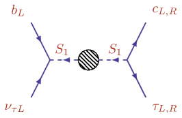
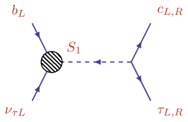
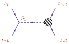
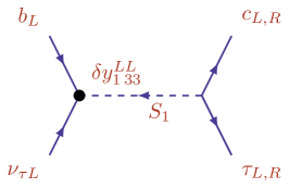
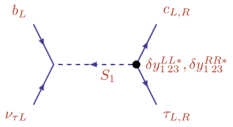
Figure 3: Radiative corrections to $b\to c\tau\nu$. The fermion self-energy diagrams are not shown. $y_{1\,33}^{LL,\rm low}$, $y_{1\,23}^{LL,\rm low}$, and $y_{1\,23}^{RR,\rm low}$ are defined by choosing the coupling counterterm in the last two diagram to cancel the loop corrections.

 

Likewise $y_{1\,33}^{LL,\rm low}$ is found from the diagrams in Fig. 3. Note that one can associate all corrections with either of the two vertices (with the LQ self-energy in the first diagram shared between them) and therefore their cancellation by the finite piece of the counterterms is well-defined. Since there are no box diagrams with two leptoquarks contributing to $b\to c\tau\nu$, the renormalized one-loop correction is zero when expressed in terms of $y_{1\,33}^{LL,\rm low}$. For this feature it is essential that there are no box diagrams with two leptoquarks contributing to $b\to c\tau\nu$. The situation is different for $b\to s\ell^{+}\ell^{-}$ for which there can be box diagrams – for instance one can exchange two $S_{1}$ LQs if one permits couplings to $s$ quarks. Thus the one-loop result for $b\to s\ell^{+}\ell^{-}$ expressed in terms of $y_{1\,33}^{LL,\rm low}$ should explicitly include these diagrams. In the standard scenarios in which the dominant effect arises from tree-level LQ exchange the smallness of the box loop makes these corrections numerically irrelevant for the scope of this work.

2.1 General pattern

We now proceed with the discussion of the radiative corrections to the decay of a LQ produced on-shell at a collider and decaying into quark and lepton. We illustrate the calculation for $y_{1\,{jk}}^{LL}\,\overline{Q^{c}_{L}}{}^{\,{j},a}\epsilon^{ab}L_{L}^{{k},b}\,S_{1}$, which drives the decays $S_{1}\to{\bar{d}_{L}^{j}\bar{\nu}_{L}^{k}}$ and $S_{1}\to{\bar{u}{}_{L}^{j}\bar{\ell}_{L}^{k}}$ (and CKM suppressed channels). For on-shell fermions the tree-level $\overline{Q^{c}}{}^{j,a}$-$L^{k,b}$-$S_{1}$ vertex amplitude reads

$$A^{\rm tree}\;=\;\textit{{}}y_{1\,jk}^{LL}\epsilon^{ab}\,\overline{u}_{j,b}{P_{L}}v_{k,a},$$ (3)

where $v_{k,a}$ ($u_{j,b}$) denotes the spinor of $L_{k}^{b}$ ($Q_{j}^{C,a}$) and there is no sum over $j,k$. To demonstrate, we first consider $(j,k)=(3,3)$ (i.e the left vertex in Fig. 3), the ratio of one-loop to tree amplitude for these decays is

$$\frac{A^{\rm one-loop}}{A^{\rm tree}} = 1\;+\;\frac{1}{2}\delta Z_{S_{1}}\;+\;\frac{1}{2}\delta Z_{Q}\;+\;\frac{1}{2}\delta Z_{L}\;+\;V_{L33}(M_{S_{1}}^{2})\;+\;\frac{\delta y_{1\,33}^{LL}}{y_{1\,33}^{LL}},$$ (4)

with the individual terms corresponding to the diagrams in Fig. 2. The proper vertex correction $V_{L33}(p^{2})$ depends on the squared $S_{1}$ momentum $p^{2}$, which is equal to $M_{S_{1}}^{2}$ here. The $S_{1}$ wave function remormalization constant (Lehmann-Symanzik-Zimmermann factor) $\delta Z_{S_{1}}$ is related to the bare self-energy $\Sigma_{S_{1}}(p^{2})$ as

$$\delta Z_{S_{1}} = \left.{-}\frac{\partial}{\partial p^{2}}\text{Re}\Sigma_{S_{1}}(p^{2})\right|_{p^{2}=M_{S_{1}}^{2}}.$$ (5)

The variables $\delta Z_{Q}$ and $\delta Z_{L}$ are the wave function constants of quark and lepton doublets, respectively. The individual contributions in Eq. (4) are ultraviolet (UV) divergent and the UV pole of $\delta y_{1\,33}^{LL}$ is chosen to render $A^{\rm one-loop}/A_{\rm tree}$ finite. For the renormalization scheme with $y_{1\,33}^{LL}=y_{1\,33}^{LL,\rm high}$ the counterterm $\delta y_{1\,33}^{LL}$ receives a finite piece such that the real part of the RHS of Eq. (4) is equal to one,

$$\frac{\delta y_{1\,33}^{LL,\rm high}}{y_{1\,33}^{LL,\rm high}} \equiv \;\left.\frac{1}{2}\,\frac{\partial}{\partial p^{2}}\mbox{Re}\,\Sigma_{S_{1}}(p^{2})\right|_{p^{2}=M_{S_{1}}^{2}}-\mbox{Re}\,V_{L33}(M_{S_{1}}^{2})-\frac{1}{2}\delta Z_{Q}\;-\;\frac{1}{2}\delta Z_{L}.$$ (6)

The imaginary part of the vertex corrections does not contribute to the decay rate $\propto|A^{\rm tree}+A^{\rm one-loop}|^{2}$ at the considered one-loop order, if the product of couplings in $A^{\rm one-loop}$ has the same phase as $y_{1\,jk}^{LL}$ entering $A^{\rm tree}$.

Repeating this procedure for $y_{1\,33}^{LL,\rm low}$ we first observe that $\Sigma_{S_{1}}(p^{2})$ and $V_{L33}(p^{2})$ enter the problem for $p^{2}=0$. The $S_{1}$ self-energy in Fig. 3 is on an internal line and we will absorb half of it into counterterms for each of the adjacent couplings. The blob in the first diagram further includes the $S_{1}$ mass counterterm with Feynman rule $-i\delta M_{S_{1}}^{2}$. For the usual “pole mass” definition $\delta M_{S_{1}}^{2}$ is chosen as

$$\delta M_{S_{1}}^{2} = \mbox{Re}\,\Sigma_{S_{1}}(M_{S_{1}}^{2}),$$

to ensure that the real part of the renormalized self-energy vanishes on-shell. Thus the ratio of one-loop to tree amplitude for $b_{L}\to\bar{\nu}_{\tau L}c_{L}\tau_{L}$ is

$$\frac{A^{\rm one-loop}}{A^{\rm tree}} = 1\;+\;\frac{\Sigma_{S_{1}}(0)-\mbox{Re}\,\Sigma_{S_{1}}(M_{S_{1}}^{2})}{M_{S_{1}}^{2}}\;+\;V_{L33}(0)\;+\;V_{L23}(0)^{*}\;+\;\frac{\delta y_{1\,33}^{LL}}{y_{1\,33}^{LL}}\;+\;\frac{\delta y_{1\,23}^{LL*}}{y_{1\,23}^{LL*}}$$ (7)

$$\;+\;\mbox{fermion wave function constants}.$$

The factor of $M_{S_{1}}^{2}$ in the denominator of the second term stems from the LQ propagator evaluated at $p^{2}=0$. The RHS of Eq. (7) vanishes for the choice

$$\frac{\delta y_{1\,33}^{LL,\rm low}}{y_{1\,33}^{LL,\rm low}} = -\;\frac{1}{2}\,\frac{\Sigma_{S_{1}}(0)-\mbox{Re}\,\Sigma_{S_{1}}(M_{S_{1}}^{2})}{M_{S_{1}}^{2}}-V_{L33}(0)-\frac{1}{2}\delta Z_{Q}\;-\;\frac{1}{2}\delta Z_{L},$$ (8)

and the analogous definition of $\delta y_{1\,23}^{LL,\rm low}$. On dimensional grounds one has $\Sigma_{S_{1}}(p^{2})\propto p^{2}$ (for our case of zero masses on internal lines), so that $\Sigma_{S_{1}}(0)=0$ and the mass counterterm $\mbox{Re}\,\Sigma_{S_{1}}(M_{S_{1}}^{2})$ dominates the self-energy diagram in Fig. 3. This is an important observation, because $\Sigma_{S_{1}}(M_{S_{1}}^{2})$ involves potentially sizable on-shell loops, while $V_{L33}(0)$ involves small loop integrals evaluated at zero external momenta. Low-energy physics probes heavy particles far below their mass shell, therefore $\mbox{Re}\,\Sigma_{S_{1}}(M_{S_{1}}^{2})$ must enter $y_{1\,33}^{LL,\rm high}/y_{1\,33}^{LL,\rm low}$ in some way. Combining Eqs. (4) and (8), inserting Eq. (5), and generalising to an arbitrary fermion pair $(j,k)$ we arrive at

$$\kappa_{1\,{jk}}^{LL} \equiv \frac{y_{1\,{jk}}^{LL,\rm high}}{y_{1\,{jk}}^{LL,\rm low}}\;=\;1\;+\;\frac{\delta y_{1\,{jk}}^{LL,\rm high}-\delta y_{1\,{jk}}^{LL,\rm low}}{y_{1\,{jk}}^{LL}},$$ (9)

$$= 1\,+\frac{1}{2}\left.\frac{\partial}{\partial p^{2}}\text{Re}\Sigma_{S_{1}}(p^{2})\right|_{p^{2}=M_{S_{1}}^{2}}\!\!\!\!-\frac{1}{2}\,\frac{\mbox{Re}\,\Sigma_{S_{1}}(M_{S_{1}}^{2})}{M_{S_{1}}^{2}}\,+V_{L{jk}}(0)\,-{\mbox{Re}\,}V_{L{jk}}(M_{S_{1}}^{2}),\quad,$$

which is a UV-finite quantity. The fermion wave function renormalization constants cancel from $\kappa_{1\,{jk}}^{LL}$, because they do not depend on the energy at which the leptoquark coupling is probed. This feature is important, because in models with several LQ copies, the diagrams with flavor-changing self-energies attached to the LQ-fermion coupling may come with couplings which are different from the tree-level coupling, permitting large corrections involving new parameters. The absence of these corrections therefore facilitates the phenomenological analyses.

2.2 Self-energies

We find the fermion loop contribution to the bare $S_{1}$ self-energy as

$$\Sigma_{S_{1}}(p^{2}) = -\sum_{l,n=1}^{3}\left[2|y_{1\ ln}^{LL}|^{2}+|y_{1\ ln}^{RR}|^{2}\right]\int\frac{d^{D}q}{(2\pi)^{D}i}\,\frac{\mbox{tr}\,\left[q\!\!\!/\;(q\!\!\!/\;+p\!\!\!/\;)P_{L}\right]}{q^{2}(p+q)^{2}}\;\quad\mbox{with }P_{L}=\frac{1-\gamma_{5}}{2},$$ (10)

$$= \sum_{l,n=1}^{3}\left[2|y_{1\ ln}^{LL}|^{2}+|y_{1\ ln}^{RR}|^{2}\right]p^{2}(4\pi)^{-D/2}\,B_{0}(p^{2};0,0),$$

in dimensional regularization with $D=4-2\epsilon$ and

$$B_{0}(p^{2};m_{1}^{2},m_{2}^{2}) \equiv \mu^{2\epsilon}\int\frac{d^{D}q}{i\pi^{D/2}}\frac{1}{(q^{2}-m_{1}^{2}+i0^{+})[(q+p)^{2}-m_{2}^{2}+i0^{+}]},$$ (11)

where $\mu$ is the renormalization scale. One then finds that

$$B_{0}(p^{2};0,0) = \frac{1}{\epsilon}+2-\gamma_{E}+i\pi-\ln\frac{p^{2}}{\mu^{2}}\;+\;{\cal O}(\epsilon),$$ (12)

and, therefore

$$\Sigma_{S_{1}}(p^{2}) = \frac{\sum_{l,n=1}^{3}\left[2|y_{1\ ln}^{LL}|^{2}+|y_{1\ ln}^{RR}|^{2}\right]}{16\pi^{2}}\,p^{2}\,\left[\frac{1}{\epsilon}+2-\gamma_{E}+\ln(4\pi)+i\pi-\ln\frac{p^{2}}{\mu^{2}}\right],$$ (13)

where $\gamma_{E}$ is the Euler-Mascheroni constant. The self-energy contribution to $\kappa_{1\,{jk}}^{LL}$ is therefore given by

$$\kappa_{1\,{jk}}^{LL,\rm self} = \frac{1}{2}\left.\frac{\partial}{\partial p^{2}}\text{Re}\Sigma_{S_{1}}(p^{2})\right|_{p^{2}=M_{S_{1}}^{2}}\!-\,\frac{1}{2}\,\frac{\mbox{Re}\,\Sigma_{S_{1}}(M_{S_{1}}^{2})}{M_{S_{1}}^{2}},$$ (14)

$$= -\frac{\sum_{l,n=1}^{3}\left[2|y_{1\ ln}^{LL}|^{2}+|y_{1\ ln}^{RR}|^{2}\right]}{32\pi^{2}},$$

contributing universally to all $S_{1}$ couplings.

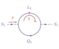
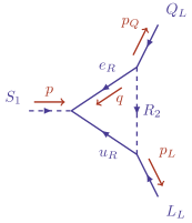
Figure 4: Diagrams for the loop correction to the $S_{1}$ LQ propagator (left) and $S_{1}$ vertex corrections to the couplings $y^{LL}_{1}$ (middle) and $y^{RR}_{1}$ (right).

 

2.3 Vertex corrections

In models which include additional LQs along with $S_{1}$, vertex corrections can involve an $R_{2}$ exchange. There are no such corrections with $S_{3}$ exchanged between the external fermion lines.

The one-loop vertex diagram reads

$$D_{Vjk}(p^{2}) = \sum_{l,n=1}^{3}y_{2\,jl}^{LR*}y_{1\,nl}^{RR}y_{2\,nk}^{RL}\,\epsilon^{ab}\,(4\pi)^{-D/2}$$

$$\times\mu^{2\epsilon}\int\frac{d^{D}q}{i\pi^{D/2}}\frac{\bar{u}_{{j}}[q\!\!\!/\;(q\!\!\!/\;+p\!\!\!/\;)]{P_{L}}v_{{k}}}{(q^{2}+i0^{+})[(q+p)^{2}+i0^{+}][(q{+}p_{Q})^{2}-M_{R_{{2}}}^{2}+i0^{+}]},$$

and we note that

$$D_{Vjk}(p^{2}){=V_{Ljk}(p^{2})A_{\rm tree}},$$ (16)

with $A_{\rm tree}$ from Eq. (3). We use $q\!\!\!/\;(q\!\!\!/\;+p\!\!\!/\;)=q^{2}+q\!\!\!/\;p\!\!\!/\;$ and define the vector three-point function as

$$C^{\rho}(p_{2},p_{3};m_{1}^{2},m_{2}^{2},m_{3}^{2}) \equiv \mu^{2\epsilon}\int\frac{d^{D}q}{i\pi^{D/2}}\frac{q^{\rho}}{[q^{2}-m_{1}^{2}][(q+p_{2})^{2}-m_{2}^{2}][(q+p_{3})^{2}-m_{3}^{2}]},$$ (17)

$$\equiv \phantom{+}p_{2}^{\rho}C_{1}(p_{2}^{2},p_{3}^{3},(p_{2}-p_{3})^{2};m_{1}^{2},m_{2}^{2},m_{3}^{2})$$

$$+\;p_{3}^{\rho}C_{2}(p_{2}^{2},p_{3}^{3},(p_{2}-p_{3})^{2};m_{1}^{2},m_{2}^{2},m_{3}^{2}).$$

Using $p_{2}=p$, $p_{3}=p_{Q}$, $p_{2}-p_{3}=p_{L}$, and $m_{3}=M_{R_{2}}$ we find

$$D_{Vjk}(p^{2}) = \sum_{l,n=1}^{3}y_{2\,jl}^{LR*}y_{1\,nl}^{RR}y_{2\,nk}^{RL}\epsilon^{ab}\,\,(4\pi)^{-D/2}.$$

$$\times\left[B_{0}(0;0,M_{R_{2}}^{2})+p^{2}C_{1}(p^{2},0,0;0,0,M_{R_{2}}^{2})\right][\overline{u}_{{j}}{P_{L}}v_{{k}}].$$

$C_{2}$ does not contribute, because in Eq. (2.3) it comes with $\overline{u}_{a,j}\not{p}_{Q}=0$ from the Dirac equation, where we neglect the mass of $Q$. For $p^{2}>0$ one finds

$$C_{1}(p^{2},0,0;0,0,M_{R_{2}}^{2})\;\stackrel{{\scriptstyle\epsilon=0}}{{=}}\;\int_{0}^{1}dy\int_{0}^{1-y}dx\frac{y}{-p^{2}xy+m_{R_{2}}^{2}(1-x-y)-i0^{+}},$$

$$=\;\frac{M_{R_{2}}^{2}}{p^{4}}\left[\mbox{Li}_{2}\Big{(}-\frac{p^{2}}{M_{R_{2}}^{2}}\Big{)}+\left(\ln\frac{p^{2}}{M_{R_{2}}^{2}}-i\pi\right)\left(\ln\Big(1+\frac{p^{2}}{M_{R_{2}}^{2}}\Big{missing})-\frac{p^{2}}{M_{R_{2}}^{2}}\right)+\frac{p^{2}}{M_{R_{2}}^{2}}\right].\qquad$$ (19)

Since $p^{2}C_{1}(p^{2},0,0;0,0,M_{R_{2}}^{2})\to 0$ for $p^{2}\to 0$, only $B_{0}(0;0,M_{R_{2}}^{2})$ contributes to $D_{V\,jk}(0)$, which, however, drops out of $V_{Lln}(0)\,-\,V_{Lln}(M_{S_{1}}^{2})$. The other vertex corrections involve the same loop integrals and can be found with trivial changes of the couplings.

2.4 Final results

Combining Eqs. (9), (14), (2.3), (16), (2.3) and (19) we get our final result for the $S_{1}$ coupling to left-handed fermions:

$$\kappa_{1\,jk}^{LL} = 1-\frac{\sum_{l,n=1}^{3}\left[2|y_{1\ ln}^{LL}|^{2}+|y_{1\ ln}^{RR}|^{2}\right]}{32\pi^{2}}\;{-}\frac{\sum_{l,n=1}^{3}y_{2\,jl}^{LR*}y_{1\,nl}^{RR}y_{2\,nk}^{RL}}{y_{1\,jk}^{LL}\,16\pi^{2}}f_{\kappa}\Big{(}\frac{M_{S_{1}}^{2}}{M_{R_{2}}^{2}}\Big{)},$$ (20)

with

$$f_{\kappa}(x) = \frac{1}{x}\,\big{[}\mbox{Li}_{2}(-x)+\ln x\,\left[\ln(1+x)-x\right]+x\big{]}.$$ (21)

The function $f_{\kappa}(x)$ vanishes for $x=0$ and is positive for $0<x<1.86$ with a maximum at $x=0.49$ and $f_{\kappa}(0.49)=0.23$. $f_{\kappa}(x)$ decreases monotonically for $x>0.49$ with $f_{\kappa}(3)=-0.24$ and $f_{\kappa}(10)=-1.17$.

By changing the couplings one immediately finds the other scaling factors:

$$\kappa_{1\,jk}^{RR} = 1-\frac{\sum_{l,n=1}^{3}\left[2|y_{1\ ln}^{LL}|^{2}+|y_{1\ ln}^{RR}|^{2}\right]}{32\pi^{2}}\;{-2}\;\frac{\sum_{l,n=1}^{3}y_{2\,jl}^{RL}y_{1\,nl}^{LL*}y_{2\,nk}^{LR*}}{y_{1\,jk}^{RR*}\,16\pi^{2}}f_{\kappa}\Big{(}\frac{M_{S_{1}}^{2}}{M_{R_{2}}^{2}}\Big{)},$$

$$\kappa_{2\,jk}^{LR} = 1-\frac{\sum_{l,n=1}^{3}\left[|y_{2\ ln}^{LR}|^{2}+|y_{2\ ln}^{RL}|^{2}\right]}{32\pi^{2}}\;-\;\frac{\sum_{l,n=1}^{3}y_{1\,jl}^{LL}y_{2\,nl}^{RL*}y_{1\,nk}^{RR*}}{y_{2\,jk}^{LR*}\,16\pi^{2}}f_{\kappa}\Big{(}\frac{M_{R_{2}}^{2}}{M_{S_{1}}^{2}}\Big{)},$$

$$\kappa_{2\,jk}^{RL} = 1-\frac{\sum_{l,n=1}^{3}\left[|y_{2\ ln}^{LR}|^{2}+|y_{2\ ln}^{RL}|^{2}\right]}{32\pi^{2}}\;-\;\frac{\sum_{l,n=1}^{3}y_{1\,jl}^{RR*}y_{2\,nl}^{LR}y_{1\,nk}^{LL}}{y_{2\,jk}^{RL}\,16\pi^{2}}f_{\kappa}\Big{(}\frac{M_{R_{2}}^{2}}{M_{S_{1}}^{2}}\Big{)},$$

$$\kappa_{3\,jk}^{LL} = 1-\frac{\sum_{l,n=1}^{3}|y_{3\ ln}^{LL}|^{2}}{16\pi^{2}}.\;$$ (22)

2.4.1 Conversion to $\mathbf{\overline{\rm MS}}$ scheme

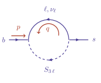
Figure 5: Diagram for the flavor-changing wave function renormalization factors induced by leptoquarks.

 

LQs in the phenomenologically interesting mass range considered in this paper are best motivated as low-energy remnants of a theory with quark-lepton unification, which is typically realized at scales between ${\cal O}(10^{3})\,\mbox{TeV}$ and the scale of grand unification (GUT scale). The construction of any viable model usually invokes the $\mathbf{\overline{\rm MS}}$ scheme for the lagrangian parameters, which are then evolved to lower scales with the RGE. Also the IR fixed-points of the RGE for the LQ couplings found in Ref. Fedele:2023rxb correspond to the $\mathbf{\overline{\rm MS}}$ scheme. In this section we present the conversion of the LQ couplings between $\mathbf{\overline{\rm MS}}$ and our “low” scheme. We exemplify this for the couplings of $S_{3\,\ell}$ for two reasons: First, in Ref. Fedele:2023rxb non-trivial RG IR fixed-points were only found for this case and second, the popular $S_{3\,\ell}$ interpretation of $b\to s\ell^{+}\ell^{-}$ data implies that the considered LQ couples to both $b$ and $s$ and therefore permits flavor-changing $b$-to-$s$ self-energy diagrams. The proper treatment of the latter diagrams in the scheme conversion deserves some explanation. As a simplification, $S_{3\,\ell}$ only couples to doublet fermion fields, leading to a more compact expression compared to the cases with other LQs.

The desired scheme conversion amounts to calculating the loop-corrected LQ-quark-lepton vertex and then determine the counterterm $\delta y_{3\,jk}^{LL}$ in both schemes, the difference fixes $y_{3\,jk}^{LL,{\rm low}}-y_{3\,jk}^{LL,\overline{{\rm MS}}}$. In any scheme one has $y_{3\,jk}^{LL,{\rm bare}}=y_{3\,jk}^{LL,{\rm scheme}}+\delta y_{3\,jk}^{LL,{\rm scheme}}$, so that

$$y_{3\,jk}^{LL,\overline{\rm MS}}-y_{3\,jk}^{LL,{\rm low}} =\;\delta y_{3\,jk}^{LL,{\rm low}}-\delta y_{3\,jk}^{LL,\overline{\rm MS}}.$$ (23)

In the “low” scheme the counterterm $\delta y_{3\,jk}^{LL,{\rm low}}$ is given in terms of the vertex and self-energy loop functions in Eq. (8).

The counterterm $\delta y_{3\,jk}^{LL,\overline{\rm MS}}$ can be obtained from Eq. (4) by retaining only the pieces proportional to $1/\epsilon-\gamma_{E}+\ln(4\pi)$ of this equation. Thus $\delta y_{3\,jk}^{LL,{\rm low}}-\delta y_{3\,jk}^{LL,\overline{\rm MS}}$ is simply found from the finite parts of the various loop contributions to $\delta y_{3\,jk}^{LL,{\rm low}}$ in Eq. (8). To this end we must calculate the wave function renormalization constants $\delta Z_{Q}$ and $\delta Z_{L}$ in both schemes, which we did not need so far because they cancel from $\kappa_{3\,jk}^{LL}$.

We start with the discussion of $\delta Z_{Q}$, which is a matrix in flavor space. For the renormalization of the $\bar{b^{c}}\ell S_{3\,\ell}$ vertex we need $\left[\delta Z_{Q}\right]_{33}$ and $\left[\delta Z_{Q}\right]_{32}$ calculated from the $b\to b$ and $b\to s$ self-energies $\Sigma_{bb}\not{p}P_{L}$ and $\Sigma_{sb}\not{p}P_{L}$, respectively. $\Sigma_{sb}$ is shown in Fig. 5. It is calculated as

$$\Sigma_{sb}\not{p}P_{L}\;=\; -3\sum_{\ell}y_{3\,3\ell}^{LL}y_{3\,2\ell}^{LL*}\,(4\pi)^{-D/2}\;\not{p}P_{L}\;B_{1}(p^{2},0,M_{S_{3\,\ell}}^{2}),$$ (24)

where

$$p^{\nu}B_{1}(p^{2},0,M_{S_{3\,\ell}}^{2})\;=\; \mu^{2\epsilon}\int\frac{d^{D}q}{i\pi^{D/2}}\frac{q^{\nu}}{(q^{2}+i0^{+})[(q+p)^{2}-M_{S_{3\,\ell}}^{2}+i0^{+}]},$$ (25)

$$B_{1}(0,0,M_{S_{3\,\ell}}^{2})\;=\; -\frac{1}{2\epsilon}-\frac{1}{4}+\frac{1}{2}\gamma_{E}+\frac{1}{2}\ln\frac{M_{S_{3\,\ell}}^{2}}{\mu^{2}}\,+{\cal O}(\epsilon).$$

Generalising the result to an arbitrary pair of quark fields, i.e. $(s,b)\mapsto(a,j)$, we find the hermitian quark-field renormalization matrix

$$\delta Z_{Q,aj}^{\overline{\rm MS}} =\frac{-3}{32\pi^{2}}\left(\frac{1}{\epsilon}-\gamma_{E}+\ln(4\pi)\right)\sum_{k=1}^{3}y_{3\,jk}^{LL}y_{3\,ak}^{LL*}.$$ (26)

For the lepton self-energy, we only consider the case where each leptoquark copy $S_{3\ell}$ only couples to one lepton generation, which we label $n$,

$$\delta Z_{L,nn}^{\overline{\rm MS}} =\frac{-3}{32\pi^{2}}\left(\frac{1}{\epsilon}-\gamma_{E}+\ln(4\pi)\right)\sum_{k=1}^{3}\left|y_{3\,kn}^{LL}\right|^{2}.$$ (27)

Using Eq. (4) with $S_{1}\to S_{3\ell}$ and Eqs. (26–27) we find

$$\delta y_{3\,jn}^{LL} =\;-y_{3\,jn}^{LL}\left[\frac{1}{2}\delta Z_{S_{3}}\;+\;\frac{1}{2}\delta Z_{L\,nn}\right]\;-\;\frac{1}{2}\sum_{k=1}^{3}\delta Z_{Q\,aj}\,y_{3\,an}^{LL},$$ (28)

and therefore,

$$\delta y_{3\,jn}^{LL,\overline{\rm MS}}=\; \frac{1}{64\pi^{2}}\,\left(\frac{1}{\epsilon}-\gamma_{E}+\ln(4\pi)\right)\times$$ (29)

$$\left[{4}\,y_{3\,jn}^{LL}\,\sum_{k=1}^{3}\left|y_{3\,kn}^{LL}\right|^{2}\;+\;3\sum_{\ell,a=1}^{3}y_{3\,j\ell}^{LL}\,y_{3\,a\ell}^{LL*}\,y_{3\,an}^{LL}\right].$$

The “low” scheme is defined such that at zero momentum transfer all loop corrections to the LQ vertex are canceled by the counterterm, rendering the tree-level result exact. To calculate $\delta y_{3\,jn}^{LL,\rm low}$ using Eq. (8) we therefore also need the finite pieces of $\Sigma_{aj}$, distinguishing the cases $a=j$ and $a\neq j$. The flavor-conserving self-energy $\Sigma_{aa}$ enters $\delta y_{3\,jn}^{LL,\rm low}$ in the same way as in $\overline{\rm MS}$, but with the full result for $B_{1}(0,0,M_{S_{3\ell}}^{2})$ given in Eq. (25). For $a\neq j$ one must instead calculate the diagram in which the tree-level $S_{3\,\ell}$ vertex is amended by $\Sigma_{aj}$ on the external quark leg (upper right diagram in Fig. 2 with $S_{1}$ replaced by $S_{3\,\ell}$ and $\nu_{\tau L}$ replaced by $L_{\ell}$). This calculation must be done keeping $m_{a}$ and $m_{j}$ non-zero, the result will contain a non-trivial dependence on the quark mass ratio $m_{j}/m_{a}$. This feature is familiar from e.g. the renormalization of the CKM matrix in the Standard Model Denner:1990yz ; Balzereit:1998id ; Gambino:1998ec ; Barroso:2000is ; Diener:2001qt ; Kniehl:2006bs . The diagram evaluates to

$$\bar{u}_{j}P_{L}v_{n}\sum_{\stackrel{{\scriptstyle\scriptstyle a=1}}{{a\neq j}}}^{3}\frac{m_{j}^{2}}{m_{j}^{2}-m_{a}^{2}}y_{3\,an}^{LL}\Sigma_{aj}(p^{2}=m_{j}^{2}).$$ (30)

In this expression we can replace $\Sigma_{aj}(p^{2}=m_{j}^{2})$ by $\Sigma_{aj}(0)$, because we discard sub-leading terms in $m_{j}^{2}/M_{S_{3\ell}}^{2}$. For the diagram with the lepton self-energy we do not encounter flavor-changing self-energies.

The final result for the desired counterterm reads

$$\delta y_{3\,jn}^{LL,\rm low} =\delta y_{3\,jn}^{LL,\overline{\rm MS}}-{\frac{1}{64\pi^{2}}}\left[{6}\sum_{\stackrel{{\scriptstyle\scriptstyle a=1}}{{a\neq j}}}^{3}\frac{m_{j}^{2}}{m_{j}^{2}-m_{a}^{2}}\sum_{\ell=1}^{3}\left(\ln\frac{M_{S_{3\ell}}^{2}}{\mu^{2}}-\frac{1}{2}\right)y_{3\,j\ell}^{LL}\,y_{3\,a\ell}^{LL*}\,y_{3\,an}^{LL}\right.$$

$$\hskip 17.07164pt\left.+{3\,y_{3\,jn}^{LL}}\sum_{\ell=1}^{3}\frac{}{}\left(\ln\frac{M_{S_{3\ell}}^{2}}{\mu^{2}}-\frac{1}{2}\right){\left|y_{3\,j\ell}^{LL}\right|^{2}}+\,y_{3\,jn}^{LL}\,\left({7}\ln\frac{M_{S_{3n}}^{2}}{\mu^{2}}-\frac{{19}}{2}\right)\sum_{a=1}^{3}\left|y_{3\,an}^{LL}\right|^{2}\right].$$ (31)

We can define a scheme transformation factor as

$$\bar{\kappa}_{3\,jn}^{LL}\equiv \,\frac{y_{3\,jn}^{LL,\rm low}}{y_{3\,jn}^{LL,\overline{\rm MS}}}\,=\,1+\frac{\delta y_{3\,jn}^{LL,\rm low}-\delta y_{3\,jn}^{LL,\overline{\rm MS}}}{y_{3\,jn}^{LL}},$$

$$= 1\,-{\frac{1}{64\pi^{2}}}\left[{6}\sum_{\stackrel{{\scriptstyle\scriptstyle a=1}}{{a\neq j}}}^{3}\frac{m_{j}^{2}}{m_{j}^{2}-m_{a}^{2}}\sum_{\ell=1}^{3}\left(\ln\frac{M_{S_{3\ell}}^{2}}{\mu^{2}}-\frac{1}{2}\right)\frac{y_{3\,j\ell}^{LL}\,y_{3\,a\ell}^{LL*}\,y_{3\,an}^{LL}}{y_{3\,jn}^{LL}}\right.$$

$$\hskip 17.07164pt\left.+{3}\sum_{\ell=1}^{3}\frac{}{}\left(\ln\frac{M_{S_{3\ell}}^{2}}{\mu^{2}}-\frac{1}{2}\right){\left|y_{3\,j\ell}^{LL}\right|^{2}}\,+\left({7}\ln\frac{M_{S_{3n}}^{2}}{\mu^{2}}-\frac{{19}}{2}\right)\sum_{a=1}^{3}\left|y_{3\,an}^{LL}\right|^{2}\right].$$ (32)

A comment is in order here: The flavor-changing self-energies renormalising the coupling $y_{3\,jn}^{LL,\rm low}$ are calculated in the phase with broken electroweak SU(2) symmetry leading to the term $m_{j}^{2}/(m_{j}^{2}-m_{a}^{2})$ in Eq. (32). This is unavoidable, because in the unbroken phase, with zero quark masses, one can arbitrarily rotate quark fields in flavor space and flavor quantum numbers are only well-defined in the broken phase. Therefore $\bar{\kappa}_{3\,jn}^{LL}$ should carry an index distinguishing down-type and up-type quarks. In practice, however, the hierarchy among quark masses allows us to set either $m_{a}$ or $m_{j}$ to zero, so that $m_{j}^{2}/(m_{j}^{2}-m_{a}^{2})$ becomes 1 or 0, and $\bar{\kappa}_{3\,jn}^{LL}$ is the same for down-type and up-type quarks in this limit. In case one wants to keep the full dependence on quark masses in Eq. (32), $m_{a}$ and $m_{j}$ must be evaluated at the same value of the renormalization scale $\mu$. (Keep in mind that the ratio $m_{j}(\mu)/m_{a}(\mu)$ is $\mu$-independent.)

Thus in the construction of a UV model of quark-lepton unification one will use $y_{3\,jn}^{LL,\overline{\rm MS}}$, subsequently run these couplings down to the scale defined by the $S_{3n}$ mass with the RG equations of Ref. Fedele:2023rxb , and finally convert the couplings to the “low” scheme by multiplying them with $\bar{\kappa}_{3\,jn}^{LL}$ for applications in flavor physics. For use in collider physics one multiplies $y_{3\,jn}^{LL,\overline{\rm MS}}$ instead with $\bar{\kappa}_{3\,jn}^{LL}\kappa_{3\,jn}^{LL}$.

3 Phenomenological implications

In order to demonstrate the impact of our results, we will outline phenomenological implications of the one-loop corrections calculated above in the context of flavor anomalies. To this end we will give numerical examples for the $\kappa$’s for values of the LQ couplings satisfying the constraints from the anomalous low-energy data. From Fig. 3 one realizes that the flavor observables constrain products of couplings while the $\kappa$’s in Eqs. (20) and (22) instead depend on the individual couplings. Therefore the deviation of the $\kappa$’s from 1 is largest if one satisfies the low-energy constraints by choosing one coupling large and the other one small. This case is most relevant for collider searches of LQ, because at first, with little statistics, one probes the parameter region with small LQ masses and large couplings. The complete one-loop corrections to LQ decay rates involving $y_{j\,ln}^{XY}$, where $XY=LL/LR/RL/RR$, are encoded in the $\kappa$’s, so that they can be considered pseudo-observables. We may study the size of the corrections, i.e. the deviation of the $\kappa$’s from 1, to assess how large the couplings $y_{j\,ln}^{XY}$ can be without spoiling perturbation theory.

3.1 Leptoquark decays

Here we consider the impact of these corrections for either explicit on-shell detection of a single LQ, or how signs of multi-LQ models may be extracted indirectly from single LQ decays. From the computation of the self energy above, we can derive the total decay width of each LQ as a function of their masses and couplings

$$\Gamma_{S_{1}} =\frac{M_{S_{1}}}{16\pi}\sum_{l,n}\left[2|y_{1\ ln}^{LL}|^{2}+|y_{1\ ln}^{RR}|^{2}\right],$$ (33)

$$\Gamma_{R_{2}} =\frac{M_{R_{2}}}{16\pi}\sum_{l,n}\left[|y_{2\ ln}^{RL}|^{2}+|y_{2\ ln}^{LR}|^{2}\right],$$ (34)

$$\Gamma_{S_{3}} =\frac{M_{S_{3}}}{8\pi}\sum_{l,n}|y_{3\ ln}^{LL}|^{2}.$$ (35)

where the indices $l,n$ run over the different decay channels. By definition, the decay of LQs is determined by the high-energy couplings $y_{j\,ln}^{XY,high}$. The implication of the $\kappa$ factors that we computed appear as a re-scaling of a LQ decay width, which in turn, modifies the predictions for the branching ratios. For example, a third-generation $S_{1}$ LQ will have modified branching ratios, for example

$$\text{BR}(S_{1}\to b\nu_{\tau}) =\frac{1}{\Gamma_{S_{1}}}\frac{M_{S_{1}}}{16\pi}|y_{1\,33}^{LL,\mathrm{high}}|^{2},$$ (36)

$$=\frac{|y_{1\,33}^{LL,\mathrm{low}}|^{2}\times|\kappa_{1\,33}^{LL}|^{2}}{\sum_{l,n}\left[2|y_{1\ ln}^{LL,\mathrm{low}}|^{2}|\kappa_{1\,ln}^{LL}|^{2}+|y_{1\ ln}^{RR,\mathrm{low}}|^{2}|\kappa_{1\,ln}^{RR}|^{2}\right]},$$

$$\text{BR}(S_{1}\to\tau t) =\frac{1}{\Gamma_{S_{1}}}\frac{M_{S_{1}}}{16\pi}(|y_{1\,33}^{LL,\mathrm{high}}|^{2}+|y_{1\,33}^{RR,\mathrm{high}}|^{2}),$$ (37)

$$=\frac{(|y_{1\,33}^{LL,\mathrm{low}}|^{2}|\kappa_{1\,33}^{LL}|^{2}+|y_{1\,33}^{RR,\mathrm{low}}|^{2}|\kappa_{1\,33}^{RR}|^{2})}{\sum_{l,n}\left[2|y_{1\ ln}^{LL,\mathrm{low}}|^{2}|\kappa_{1\,ln}^{LL}|^{2}+|y_{1\ ln}^{RR,\mathrm{low}}|^{2}|\kappa_{1\,ln}^{RR}|^{2}\right]},$$

where we have neglected phase space effects, as $m_{t}^{2}/m_{S_{1}}^{2}$ can barely exceed 2%. In order to calculate the impact of a model built for low scale observables on the direct production rates at colliders then one should incorporate these radiative corrections.

To determine the hierarchy between the couplings, one can measure the ratio of branching ratios, for example

$$\frac{\text{BR}(S_{1}\to\tau t)}{\text{BR}(S_{1}\to\nu_{\tau}b)} \approx\frac{|y_{1\,33}^{LL,\mathrm{high}}|^{2}+|y_{1\,33}^{RR,\mathrm{high}}|^{2}}{|y_{1\,33}^{LL,\mathrm{high}}|^{2}}.$$ (38)

From this observable we note the following relation between low- and high-energy couplings

$$\frac{|y_{1\,33}^{LL,\mathrm{high}}|^{2}+|y_{1\,33}^{RR,\mathrm{high}}|^{2}}{|y_{1\,33}^{LL,\mathrm{high}}|^{2}}=\frac{|y_{1\,33}^{LL,\mathrm{low}}|^{2}|\kappa_{1\,33}^{LL}|^{2}+|y_{1\,33}^{RR,\mathrm{low}}|^{2}|\kappa_{1\,33}^{RR}|^{2}}{|y_{1\,33}^{LL,\mathrm{low}}|^{2}|\kappa_{1\,33}^{LL}|^{2}}.$$ (39)

In the absence of an additional LQ $R_{2}$, it follows from Eqs. (20) and (22) that $\kappa_{1\,33}^{RR}=\kappa_{1\,33}^{LL}$, i.e. the radiative corrections to the right- and left-handed couplings are equal and

$$\frac{\text{BR}(S_{1}\to\tau t)}{\text{BR}(S_{1}\to\nu_{\tau}b)} \approx\frac{|y_{1\,33}^{LL,\mathrm{low}}|^{2}+|y_{1\,33}^{RR,\mathrm{low}}|^{2}}{|y_{1\,33}^{LL,\mathrm{low}}|^{2}},$$ (40)

which suggests that the ratio of couplings is insensitive to radiative corrections. However, the presence of $R_{2}$ may break this relation, which implies that this ratio can act as an indirect probe of the the presence of a second LQ with sizeable couplings.

3.2 Flavour anomalies

Several measured branching ratios and decay distributions have hinted at the presence of BSM physics influencing the branching ratios of $b\to s\ell\ell$ and $b\to c\ell\nu$. Notably in the neutral current process these are driven by the decay $b\to s\mu\mu$, where there is a deficit in events in the kinematic region $q^{2}\leq 8$ GeV LHCb:2014cxe ; LHCb:2015wdu ; LHCb:2021zwz ($q^{2}$ is the invariant mass of the lepton pair), in contrast with the SM predictions of Refs. Khodjamirian:2010vf ; Khodjamirian:2012rm . The angular observable $P_{5}^{\prime}$, which parameterizes the angular distribution of final states in $B\to K^{*}\mu^{+}\mu^{-}$, also follows this trend LHCb:2013ghj ; LHCb:2015svh ; LHCb:2020lmf ; LHCb:2020gog . Measurements of the lepton flavor universality (LFU) ratios Hiller:2003js

$$R_{K^{(*)}}=\frac{\text{BR}(B\to K^{(*)}\mu^{+}\mu^{-})}{\text{BR}(B\to K^{(*)}e^{+}e^{-})},$$ (41)

presently show a compatibility with the SM predictions $R_{K^{(*)}}\simeq 1$ LHCb:2022qnv ; LHCb:2022vje , indicating that the BSM physics invoked to explain the anomalous data in $b\to s\mu^{+}\mu^{-}$ should couple with similar strengths to electrons and muons. For the charged-current process, a long-standing anomaly is observed in the LFU ratios

$$R_{D^{(*)}}=\frac{\text{BR}(B\to D^{(*)}\tau\nu)}{\text{BR}(B\to D^{(*)}\ell\nu)}\quad\ell\in\{e,\mu\}.$$ (42)

The HFLAV collaboration combines six separate measurements from BaBar BaBar:2012obs , Belle Belle:2015qfa ; Belle:2016ure ; Belle:2019rba , and LHCb LHCb:2023zxo ; LHCb:2023uiv to give the following average values, as per Summer 2023 HFLAV:2022esi

$$R_{D}^{\text{HFLAV}}=0.357\pm 0.029,\qquad\;\;\;\;R_{D^{*}}^{\text{HFLAV}}=0.284\pm 0.012,$$ (43)

with a correlation coefficient of $\rho=-0.37$. To be compared with the theoretical values

$$R_{D}=0.298\pm 0.004,\qquad\;\;\;\;R_{D^{*}}=0.254\pm 0.005,$$ (44)

resulting in a theory/experiment discrepancy of $3.2\sigma$

Improved sensitivity to the $D^{*}$ and $\tau$ polarizations can discriminate between different BSM explanations of these anomalies, and complementary information can be garnered from the ratio $R_{\Lambda_{c}}\equiv\text{BR}(\Lambda_{b}\to\Lambda_{c}\tau\nu)/\text{BR}(\Lambda_{b}\to\Lambda_{c}\ell\nu)$ Blanke:2018yud ; Blanke:2019qrx . For a BSM explanation for $R_{D^{(*)}}$ to be consistent with the latter, future measurement of $R_{\Lambda_{c}}$ must move upwards from the 2022 value $R_{\Lambda_{c}}^{\text{LHCb}}=0.242\pm 0.026\pm 0.040\pm 0.059$ LHCb:2022piu to $R_{\Lambda_{c}}=0.39\pm 0.05$ Fedele:2022iib , to be consistent with Eq. (43).

These flavor anomalies may be addressed by a combination of the scalar LQs $S_{1},R_{2}$ and $S_{3}$ (a $SU(2)$ singlet, doublet and triplet, respectively). The LQs $S_{1}$ and $R_{2}$ are capable of explaining the flavor anomalies with tree-level contributions to $b\to c\tau\nu$, and $S_{3}$ to $b\to s\mu\mu$. In order to be consistent with LFU, i.e. Eq. (41), one requires multiple copies of $S_{3}$ in order to consistently explain $b\to s\ell\ell$ data and to avoid constraints from lepton flavor violating decays, e.g. $\mu\to e\gamma$. Therefore this motivates extensions to the SM involving the combinations $(S_{1},S_{3\,\ell})$ or $(R_{2},S_{3\,\ell})$, each with at least two copies of $S_{3}$ of the triplet LQ (denoted $S_{3\,\ell}$) with $S_{3\,e}$ and $S_{3\,\mu}$ exclusively coupling to $e$ and $\mu$, respectively. We do not perform any phenomenological analysis of constraints on these models here, but simply use the best-fit values of the Wilson coefficients from the literature to employ realistic scenarios for the LQ couplings and masses in our numerical examples. We draw the readers’ attention to Ref. Fedele:2023rxb and references therein for further discussion of constraints.

3.2.1 Scalar singlet

As discussed above, the singlet $S_{1}$ is capable of generating tree-level contributions to $b\to c\tau\nu$. We adopt a minimal coupling scenario for the $S_{1}$ scalar LQ choosing nonzero values only for the couplings $y_{1\,33}^{LL}$ and $y_{1\,23}^{RR}$. The contributions to $b\to c\ell\nu_{\ell}$ are given by the following effective interactions, expressed in the flavio basis Straub:2018kue for the Weak Effective Theory (WET), where

$$\mathcal{L}=\mathcal{L}_{\text{SM}}-\frac{4G_{F}}{\sqrt{2}}V_{cb}\sum_{b\to c\tau\nu}C_{i}\mathcal{O}_{i},$$ (45)

with the sum indicating a sum over the operator basis for the process $b\to c\tau\nu$. The operators of interest are

$$\mathcal{O}_{S_{L}}=(\overline{c}P_{L}b)(\overline{\tau}P_{L}\nu_{\tau}),\quad\quad\mathcal{O}_{T}=(\overline{c}\sigma^{\mu\nu}P_{L}b)(\overline{\tau}\sigma_{\mu\nu}P_{L}\nu_{\tau}),$$ (46)

$$\mathcal{O}_{V_{L}}=(\overline{c}\gamma^{\mu}P_{L}b)(\overline{\tau}\gamma_{\mu}P_{L}\nu_{\tau}).$$

Here, $G_{F}$ is the Fermi constant, and $V_{ij}$ is the SM CKM matrix elements. Note that here we have restricted ourselves to lepton-flavor conserving effective interactions. This minimal scenario will generate the following nonzero WCs, where we have assumed the LQ couplings to be real-valued

$$C_{S_{L}}(M_{S_{1}}) =-4C_{T}(M_{S_{1}})=-\frac{1}{4\sqrt{2}G_{F}V_{cb}M_{S_{1}}^{2}}y_{1\,23}^{RR}y_{1\,33}^{LL},$$ (47)

$$C_{V_{L}}(M_{S_{1}}) =\frac{1}{4\sqrt{2}G_{F}M_{S_{1}}^{2}}(y_{1\,33}^{LL})^{2}.$$ (48)

We recall we have adopted the down-aligned mass basis for the quarks, see Eq. Eq. (2). These LQ couplings can be chosen to be fixed in the low-scale renormalization scheme.

A recent fit to these WCs in a model-dependent study of the anomalies $R_{D^{(*)}}$ and other $b\to c\tau\nu$ observables can be found in Ref. Iguro:2022yzr . Their results yield the following best fits to single scalar/tensor WCs, evaluated at $\mu_{b}$,

$$C_{S_{L}}=-8.9C_{T}=0.19$$ (49)

which, when evolved according to Appendix A, corresponds to $C_{S_{L}}=-4C_{T}\approx 0.095$ at $M_{S_{1}}=2$ TeV. Although this fit was performed prior to the most recent updates to the $R_{D^{*}}$ measurements, it remains compatible with the central values of the present HFLAV fit HFLAV:2022esi to these anomalies within roughly $1.3\sigma$. Matching onto Eq. (47), this corresponds to

$${y_{1\,23}^{RR}\,y_{1\,33}^{LL}}\approx-1.06\;$$ (50)

for a LQ mass of $2$ TeV.

A fit to the anomalous $R_{D^{*}}$ measurements arising solely from the $C_{V_{L}}$ in the $S_{1}$ model is ruled-out primarily due to large contributions to $b\to s\nu\bar{\nu}$ (see Appendix B) which are ruled-out by present measurements. In the framework prescribed above, it is impossible to avoid nonzero contributions to the $C_{V_{L}}$ coefficient, although it is CKM suppressed. For this reason, we elect for a larger value for $y^{RR}_{1\,23}$ to minimize the effect from the vector WC. Dominant constraints on this coupling come from high-$p_{T}$ probes of the effective coupling in $c\bar{c}\to\tau\bar{\tau}$ interactions, resulting in a constraint $|y^{RR}_{1\,23}|<2.6$ for a $2$ TeV leptoquark mass Angelescu:2018tyl ; Bigaran:2022kkv . Saturating this upper bound corresponds to a candidate point $(y_{1\,23}^{RR},y_{1\,33}^{LL})=(2.6,-0.41)$. For this point, $C_{V_{L}}$ has negligible impact on the values for $R_{D^{(*)}}$, meaning that this point is still able to fit the anomalies while being safe from constraints. Matching onto Eq. (47), this point is found to yield a value of

$$\kappa_{1\,jk}^{LL}=\kappa_{1\,jk}^{RR}=1-\frac{2|y^{LL}_{1\,33}|^{2}+|y^{RR}_{1\,23}|^{2}}{32\pi^{2}}\approx 0.98,$$ (51)

and in the scalar singlet LQ model to explain the anomalies in $b\to c\tau\nu$ this correction corresponds to a $2\%$ effect. Therefore, the high energy Yukawa coupling relevant for on-shell production of the $S_{1}$ LQ is 98% of the value of that at low-energy.

3.2.2 Scalar doublet

Following similarly from Eqs. (46) and  (45), the doublet $R_{2}$ generates the following nonzero WCs for contributing to the $b\to c\tau\nu$ process, this time not assuming real-valued LQ couplings 

$$C_{S_{L}}(M_{R_{2}}) =4C_{T}(M_{R_{2}})=\frac{1}{4\sqrt{2}G_{F}V_{cb}M_{R_{2}}^{2}}y^{LR\;*}_{2\;33}y^{RL}_{2\;23}.$$ (52)

Following again from the fit in Ref. Iguro:2022yzr , the following best fit to single scalar/tensor WCs, evaluated at $\mu_{b}$,

$$C_{S_{L}}=8.4C_{T}\approx-0.07\pm 0.58\,i,$$ (53)

which, when evolved according to Appendix A, corresponds to $C_{S_{L}}\approx 8.4C_{T}=-0.039\pm 0.319\,i$ at $M_{R_{2}}=2$ TeV. Matching onto Eq. (52), this corresponds to

$${y^{LR\;*}_{2\;33}y^{RL}_{2\;23}}\approx-0.41\pm 3.43\,i\;,$$ (54)

again for a LQ mass of $2$ TeV. Dominant constraints on these couplings arise from a loop-order corrections to $Z\to\tau\overline{\tau}$ couplings and the high-$p_{T}$ dilepton and monolepton tails of proton collisions.

The light-quark couplings to taus are limited by constraints on the flavor-conserving, non-universal, contact interactions in $pp\to\tau^{+}\tau^{-}$ and $pp\to\tau\nu$ (+ soft jets)Faroughy:2016osc ; Greljo:2017vvb ; Angelescu:2018tyl . Utilising the program HighPT Allwicher:2022mcg ; Allwicher:2022gkm to extract these constraints and mapping the result onto the above model, we find that requiring agreement at 3(2)$\sigma$ constrains $|C_{S_{L}}|\lesssim 0.68(0.57)$ for a $2$ TeV LQ mass. This is consistent with Ref. Becirevic:2024pni where they examine the $R_{2}$ model and conclude that these constraints are incompatible with an $R(D^{(*)})$ if the high-$p_{T}$ constraints are taken at $2\sigma$, although they note that these constraints should be treated with caution due to uncertainties from $\tau$ reconstruction Jaffredo:2021ymt . We conservatively take the $3\sigma$ constraint and retain the above point as valid, as assessing the definite validity is beyond the scope of this work.

For $Z\to\tau\overline{\tau}$, the coupling of the LQ to the tau and top quarks $\approx y^{LR}_{2\,33}$ generates a enhanced correction Becirevic:2018uab . A representative coupling assignment which satisfies this constraint (see Appendix B) is $(y^{LR}_{2\;33},y^{RL}_{2\;23})\approx(0.5,-0.82\pm 6.86\,i)$, corresponds to

$$\kappa_{2\,jk}^{LR}=\kappa_{2\,jk}^{RL}=1-\frac{|y^{LR}_{2\,33}|^{2}+|y^{RL}_{2\,23}|^{2}}{32\pi^{2}}\approx 0.85.$$ (55)

So, for the scalar doublet LQ model to explain the anomalies in $b\to c\tau\nu$ this correction corresponds to a $15\%$ effect and the high energy Yukawa coupling relevant for on-shell production of the $R_{2}$ LQ is 85% of the value of that at low-energy. Of course the large deviation from 1 in Eq. (55) stems from our choice with $|y^{RL}_{2\;23}|\gg|y^{LR}_{2\;33}|$. If chose $|y^{RL}_{2\;23}|\approx|y^{LR}_{2\;33}|\approx 1.86$ instead, we’d find $\kappa_{2\,jk}^{LR}=\kappa_{2\,jk}^{RL}=0.98$ instead. Yet, as stated at the beginning of this section, collider searches first probe the large-couplings region and Eq. (55) shows that the corrections encodes in our $\kappa$’s matter here. We also verify that LQ couplings as large as seven do not lead to excessive corrections which would put the validity of perturbation theory into doubt.

3.2.3 Scalar triplet

The scalar triplet is relevant for addressing anomalies in $b\to s\ell\ell$. The effective Lagrangian parameterizing these transitions is given by

$$\mathcal{L}=\mathcal{L}_{\text{SM}}-\frac{4G_{F}}{\sqrt{2}}V_{tb}V_{ts}^{*}\left(C_{9}^{\ell}\mathcal{O}_{9}^{\ell}+C_{10}^{\ell}\mathcal{O}_{10}^{\ell}\right)+\text{h.c.},$$ (56)

and the operators are given by

$$\mathcal{O}^{\ell}_{9}=\frac{\alpha_{\text{em}}}{4\pi}\left(\overline{s}\gamma_{\mu}P_{L}b\right)\left(\overline{\ell}\gamma^{\mu}\ell\right),\;\;\;\;\;\mathcal{O}_{10}^{\ell}=\frac{\alpha_{\text{em}}}{4\pi}\left(\overline{s}\gamma_{\mu}P_{L}b\right)\left(\overline{\ell}\gamma^{\mu}\gamma_{5}\ell\right).$$ (57)

Here, $\alpha_{\text{em}}$ is the fine structure constant.

Matching the scalar triplet LQ model onto this Lagrangian gives the following contribution

$$C^{\ell}_{9}(M_{\text{LQ}})=-C^{\ell}_{10}(M_{\text{LQ}})=-\frac{\pi}{2\sqrt{2}G_{F}V_{tb}V_{ts}^{*}\alpha_{\text{em}}}\frac{y^{LL}_{3\,3\ell}y^{LL\;*}_{3\,2\ell}}{M_{S_{3}}^{2}}.$$ (58)

For the triplet LQ it is useful to define the quantity $C^{\ell}_{L}=C_{9}^{\ell}=-C_{10}^{\ell}$, and recent global fits show a preference for a universal assignments of these WCs such that $C^{U}_{L}=C^{e}_{L}=C^{\mu}_{L}=C^{\tau}_{L}\approx-0.4$ Ciuchini:2022wbq ; Greljo:2022jac ; Alguero:2023jeh .

We begin by considering a single triplet, $S_{3}$, with lepton-universal couplings. Recalling that $C^{U}_{L}$ as a vector coefficient does not run in QCD, this corresponds to

$$y^{LL}_{3\,3\ell}y^{LL\;*}_{3\,2\ell}\approx-0.0055[-0.14],$$ (59)

for a LQ mass of $2$ TeV [10 TeV]. Note that for the corrections to the Yukawa couplings $\kappa^{LL}_{3,\,jk}$ are generated uniformly in flavor space $(j,k)$ because they are each sourced by the LQ self-energy. For $\kappa^{LL}_{3,\,jk}$ to correspond to a $30\%$ effect relies on a coupling assignment for a LQ mass of $2$ TeV of $(y^{LL}_{3\,3\ell},y^{LL}_{3\,2\ell})\approx(6.1,-10^{-3})$ and for a LQ mass of $10$ TeV of $(y^{LL}_{3\,3\ell},y^{LL}_{3\,2\ell})\approx(6.1,-0.023)$. Therefore in each of these instances the high-energy, lepton-universal, Yukawa coupling relevant for on-shell production of the $S_{3}$ LQ is 70% of the value of that at low-energy.

3.2.4 A comment on models with multiple LQ

The models considered in Section 3.2 all involve the addition of one LQ at a time and so their corrections are dominated by the LQ self-energies. However, the results from Section 2.4 illustrate that the largest and most interesting effects will occur when two LQs are present in a model: namely, in models with both $S_{1}$ and $R_{2}$ present. In this model, the Lagrangian in Eq. (1) reduces to

$$\mathcal{L}_{\rm LQ} = \phantom{+\;}y_{1\,jk}^{LL}\,\overline{Q^{c}_{L}}{}^{j,a}\,\epsilon^{ab}L_{L}^{k,b}\,S_{1}\;+\;y_{1\,jk}^{RR}\,\overline{u_{R}^{c}}{}^{j}e_{R}^{k}\,S_{1}$$ (60)

$$-\;y_{2\,jk}^{RL}\,\overline{u_{R}}^{j}\epsilon^{ab}L_{L}^{k,b}\,R_{2}^{a}\quad\;+\;y_{2\,jk}^{LR}\,\overline{Q_{L}}{}^{j,a}e_{R}^{k}\,R_{2}^{a}\;+\;\mbox{h.c.}.$$

The LQs $S_{1}$ and $R_{2}$ are particularly phenomenologically interesting because they are the sole two mixed-chiral scalar LQs: they have couplings to both right- and left-handed quarks and leptons. These leptoquarks have been exploited in the literature, for example, to generate large contributions to chirality-flipping dipole operator corrections, responsible for radiative mass generation and large dipole moments for charged leptons (see e.g. Refs. Bigaran:2020jil ; Bigaran:2021kmn ). Nevertheless, these models do not necessarily require both LQs at once. However, future measurements of lepton CLFV and associated processes may necessitate such model building in the near future.

A particularly interesting feature of the results in Section 3.2 is an inverse dependence of the vertex correction on the low-scale LQ coupling being corrected. This means that even a small low-scale coupling can have a large correction, simply because the tree-level coupling is suppressed or even absent in the loop vertex diagram, which involves three different couplings instead. Take for example a LQ model with both $S_{1}$ and $R_{2}$ and consider the correction to the coupling $y_{1\,jk}^{RR*}$, taking LQ masses such that $f({M_{S_{1}}^{2}}/{M_{R_{2}}^{2}}=10)=-1.17$. Fixing each of the LQ couplings to third-generation quarks to $0.1$ aside from the LQ coupling we are correcting for the purpose of demonstration,

$$\kappa_{1\,jk}^{RR}=1-3\,|y_{1\,jk}^{RR*}|^{2}\times 10^{-3}+\;\frac{4.4\times 10^{-5}}{y_{1\,jk}^{RR*}}.$$ (61)

Therefore, for a LQ coupling $y_{1\,jk}^{RR*}\approx 10^{-4}$ the correction is $\kappa_{1\,jk}^{RR}\approx 1.44$, corresponding to a correction of $44\%$ to this coupling.

3.3 Unification and IR fixed-points

Leptoquarks particularly appear in theories that unify quarks and leptons, although the unification scale $M_{\text{QLU}}$ is often many orders of magnitude above the LQ mass scale. If we assume that the mass-gap between the electroweak scale and $M_{\text{QLU}}$ is populated only by LQs and SM particles, one may use renormalization-group evolution of LQ couplings to fermions up to this scale. This analysis was performed in Ref. Fedele:2023rxb . The scale $M_{\text{QLU}}$ determines the masses of any remaining particles in the unification framework, and the effects of these particles decouple for a scalar LQ model as $M_{\text{QLU}}\to\infty$ .

In Ref. Fedele:2023rxb it has been found that the Yukawa couplings of a model with three scalar triplet LQ carrying lepton flavor number features IR fixed-points withemergent lepton flavor universality in their RG evolution from some high scale down to $M_{LQ}$. This feature persists if additional LQs (such as $S_{1}$) are present. Since beta functions are derived in mass independent renormalization schemes, typically $\overline{\mathrm{MS}}$, the couplings must be converted to the ‘low’ or ‘high’ scheme for use in phenomenological applications.

Taking $M_{S_{3}}{\equiv}M_{S_{3\,e}}=M_{S_{3\,\mu}}=M_{S_{3\,\tau}}{=}14.2$ TeV and the IR fixed-point couplings in Table 1. reproduces the $b\to s\ell^{+}\ell^{-}$ data. In each case the conversion between low-energy and high-energy couplings is given by

$$\kappa_{3\,jk}^{LL} =1-\left(\frac{|y^{LL}_{3\,3\ell}|^{2}+|y^{LL}_{3\,2\ell}|^{2}}{16\pi^{2}}\right)\approx 0.996,$$ (62)

where we recall each LQ only couples to one lepton flavor, $\ell$, at a time. We multiply $y_{3\,jn}^{LL,\overline{\rm MS}}$ with ${\bar{\kappa}_{3\,jn}^{LL}}$. to convert to the ‘low’ scheme, and these conversion factors and the corresponding low-energy couplings are given in Table 1. We evaluate the $\overline{\text{MS}}$ conversion factor at $\mu=M_{S_{3}}$.

Benchmark	$S_{3\ell}$	$(y^{LL,\overline{\text{MS}}}_{3\,2\ell},y^{LL,\overline{\text{MS}}}_{3\,3\ell})$	$(\bar{\kappa}_{3\,2\ell}^{LL}\kappa_{3\,2\ell}^{LL},\bar{\kappa}_{3\,3\ell}^{LL}\kappa_{3\,3\ell}^{LL})$	$(y^{LL,\text{low}}_{3\,2\ell},y^{LL,\text{low}}_{3\,3\ell})$
A	$S_{3\,e}$	$(0.760,0.189)$	$(1.007,1.008)$	$(0.765,0.191)$
	$S_{3\,\mu}$	$(0.191,0.759)$	$(1.005,1.006)$	$(0.192,0.764)$
	$S_{3\,\tau}$	$(0.639,-0.452)$	$(1.006,1.011)$	$(0.643,-0.457)$
B	$S_{3\,e}$	$(0.189,0.760)$	$(1.007,1.007)$	$(0.190,0.765)$
	$S_{3\,\mu}$	$(0.759,0.191)$	$(1.007,1.008)$	$(0.764,0.193)$
	$S_{3\,\tau}$	$(0.639,-0.452)$	$(1.006,1.011)$	$(0.643,-0.457)$

Table 1: Benchmark points from Ref. Fedele:2023rxb , converted to the low-scheme utilising our formalism.

Although $\bar{\kappa}_{3\,jk}^{LL}$ deviates from 1 more than $\kappa_{3\,jk}^{LL}$, the effects in Table 1 are still small, because the fixed-point values of the couplings are moderate in size. In general, however, the first term in the square bracket in Eq. (32) can give a large contribution, if the tree-level coupling is small.

4 Conclusions

Leptoquark (LQ) phenomenology involves the combination of constraints from low and high energy. The former are inferred from solutions to the flavor anomalies, while the latter are found from LHC bounds on production cross sections. Stronger collider bounds, pushing the LQ masses to higher values, imply larger couplings in the LQ lagrangian in Eq. (1) to explain anomalous low-energy data. Sizable couplings, however, lead to potentially large loop corrections with LQs. We have studied such corrections for the popular $S_{1}$, $R_{2}$, and $S_{3}$ LQ scenarios with the following results:

(1)  The radiative corrections have a particularly simple structure, as they can be completely absorbed into a renormalization of the LQ coupling. This allows us to define two renormalization schemes designed for low-energy and high-energy observables. With the choice of our ‘low’ scheme all considered corrections are absorbed into the coupling $y_{n\,jk}^{XY,\mathrm{low}}$, so that the tree and one-loop amplitudes for the studied flavor-changing processes coincide. The same feature holds for the LQ decay amplitudes in the ‘high’ scheme. The combination of low-energy and high-energy data only involves the conversion factors $\kappa_{n,jk}^{XY}\equiv y_{n\,jk}^{XY,\mathrm{high}}/y_{n\,jk}^{XY,\mathrm{low}}$. While this method captures all radiative corrections to both the low-energy process and the LQ decay amplitude, a full one-loop calculation of the production cross sections involves additional diagrams with process-dependent corrections and the use of $y_{n\,jk}^{XY,\mathrm{high}}$ in the tree result only captures a universal subset, but permit simulations with tree-level event generators.

(2) In scenarios with only one LQ species the $\kappa_{n,jk}^{XY}$ have a particularly simple structure, originating solely from self-energies, and are always proportional to the tree-level coupling. In these scenarios one always finds $\kappa_{n,jk}^{XY}<1$, implying that collider constraints are weakened. Only scenarios with both $S_{1}$ and $R_{2}$ involve vertex corrections, which moreover involve different couplings compared to tree level and can therefore be enhanced if the tree coupling is small.

(3)  Our calculations resulted in unexpectedly small loop functions, so that the $\kappa_{n,jk}^{XY}$ are close to 1 for $y_{n\,jk}^{XY}={\cal O}(1)$. The LQ scenarios explaining the $b\to c\tau\bar{\nu}$ and $b\to s\ell^{+}\ell^{-}$ anomalies involve two couplings. In the $S_{1}$ and $S_{3}$ scenarios ${\cal O}(1)$ couplings are compatible with LQ masses satisfying collider bounds and the $\kappa_{n,jk}^{XY}$’s can be neglected. However, for hierarchical choices of these couplings, with one coupling much larger than the other, $\kappa_{n,jk}^{XY}$ can be substantially smaller than 1.

(4)  The smallness of the loop functions implies that perturbation theory works for couplings larger than 5. This feature opens up the parameter spaces, because low-energy data can be explained with large LQ masses and furthermore $\kappa_{n,jk}^{XY}<1$ weakens the collider bounds.

(5)  Like the vertex corrections mentioned in item (2) also flavor-changing fermion self-energies need not involve the tree-level coupling. While these self-energies drop out from the $\kappa_{n,jk}^{XY}$’s, they contribute to the scheme conversion from $\overline{\rm MS}$ to either ‘low’ or ‘high’ scheme. The corresponding scheme transformation factors $\bar{\kappa}_{n,jk}^{XY}$ are larger than the $\kappa_{n,jk}^{XY}$’s, but can still be omitted for the choices of the infrared fixed-point solutions for $y_{3\,jk}^{LL,\overline{\mathrm{MS}}}$ found in Ref. Fedele:2023rxb .

(6)  Irrespective of any low-energy data, collider searches first probe the parameter region with smallest masses and largest couplings. These searches will constrain $y_{n\,jk}^{XY,\mathrm{high}}$ and if these bounds are used in other schemes the couplings must be converted properly, e.g. the $\overline{\rm MS}$ values are found by dividing $y_{n\,jk}^{XY,\mathrm{high}}$ with $\bar{\kappa}_{n,jk}^{XY}\kappa_{n,jk}^{XY}$.

Appendix A Wilson coefficient evolution

In Ref. Iguro:2022yzr , the fit of the WCs to $b\to c\tau\nu$ is done at the scale $\mu_{b}=4.8$ GeV, which must then be evolved to the scale $m_{\text{LQ}}$ to be matched onto the full theory. The QCD renormalization-group equations (RGEs) Jenkins:2013wua ; Alonso:2013hga ; Gonzalez-Alonso:2017iyc (first matrix) and the LQ-charge independent QCD one-loop matching Aebischer:2018acj (second matrix) give the following relation for $M_{\text{LQ}}=2$ TeV

$$\begin{pmatrix}C_{V_{L}}(\mu_{b})\\ C_{V_{R}}(\mu_{b})\\ C_{S_{L}}(\mu_{b})\\ C_{S_{R}}(\mu_{b})\\ C_{T}(\mu_{b})\end{pmatrix} \approx\begin{pmatrix}1&0&0&0&0\\ 0&1&0&0&0\\ 0&0&1.82&0&-0.35\\ 0&0&0&1.82&0\\ 0&0&-0.004&0&0.83\\ \end{pmatrix}\begin{pmatrix}1.12&0&0&0&0\\ 0&1.07&0&0&0\\ 0&0&{1.05}&0&0\\ 0&0&0&{1.10}&0\\ 0&0&0&0&1.07\\ \end{pmatrix}\begin{pmatrix}C_{V_{L}}(M_{\text{LQ}})\\ C_{V_{R}}(M_{\text{LQ}})\\ C_{S_{L}}(M_{\text{LQ}})\\ C_{S_{R}}(M_{\text{LQ}})\\ C_{T}(M_{\text{LQ}})\end{pmatrix},$$

$$\approx\begin{pmatrix}1.12&0&0&0&0\\ 0&1.07&0&0&0\\ 0&0&1.91&0&-0.38\\ 0&0&0&2.00&0\\ 0&0&0&0&0.89\\ \end{pmatrix}\begin{pmatrix}C_{V_{L}}(M_{\text{LQ}})\\ C_{V_{R}}(M_{\text{LQ}})\\ C_{S_{L}}(M_{\text{LQ}})\\ C_{S_{R}}(M_{\text{LQ}})\\ C_{T}(M_{\text{LQ}})\end{pmatrix},$$ (63)

from which we obtain $C_{S_{L}}(\mu_{b})\approx-8.9C_{T}(\mu_{b})$ for $S_{1}$ and $C_{S_{L}}(\mu_{b})\approx 8.4C_{T}(\mu_{b})$ for $R_{2}$.

Appendix B Brief comment on constraints

We briefly comment on constraints relevant for electing benchmark points.

B.1 Constraints from $b\to s\nu\bar{\nu}$

The contribution of BSM to $b\to s\nu\overline{\nu}$ transitions may be parameterized by the following, in the absence of significant right-handed vector currents Buras:2014fpa

$$\mathcal{L}^{\nu\bar{\nu}}\supset\frac{4G_{F}}{\sqrt{2}}V_{tb}V_{ts}^{*}C_{\nu\bar{\nu}}^{\ell}\left[\frac{\alpha_{\text{em}}}{4\pi}(\bar{s}\gamma_{\mu}P_{L}b)(\bar{\nu}_{\ell}\gamma^{\mu}(1-\gamma_{5})\nu_{\ell})\right]+\text{h.c.}.$$ (64)

As collider experiments do not distinguish between neutrino flavors, the sum over all flavors appears in the ratio of branching fractions and its SM prediction

$$R_{K^{(*)}}^{\nu\bar{\nu}}=\frac{\text{Br}^{\text{exp}}(B\to K^{(*)}\nu\bar{\nu})}{\text{Br}^{\text{SM}}(B\to K^{(*)}\nu\bar{\nu})}=\frac{(C_{\nu\bar{\nu}}^{\text{SM}}+C_{\nu\bar{\nu}}^{e})^{2}+(C_{\nu\bar{\nu}}^{\text{SM}}+C_{\nu\bar{\nu}}^{\mu})^{2}+(C_{\nu\bar{\nu}}^{\text{SM}}+C_{\nu\bar{\nu}}^{\tau})^{2}}{3(C_{\nu\bar{\nu}}^{\text{SM}})^{2}},$$ (65)

where $C_{\nu\bar{\nu}}^{\text{SM}}\approx-6.35$. The experimental limits from the Belle collaboration read $R_{K}^{\nu\bar{\nu}}<3.9$ and $R_{K^{*}}^{\nu\bar{\nu}}<2.7$ at 90% C.L.Belle:2017oht . The recent Belle-II measurement of Br($B^{+}\to K^{+}+\text{inv.})=(2.4\pm 0.7)\times 10^{-5}$Belle-II:2023esi , assuming three-body decay with massless neutrinos, may be contrasted with the SM prediction for this branching ratio, $\text{Br}^{\text{SM}}(B^{+}\to K^{+}\nu\bar{\nu})=(2.81\pm 0.15)\times 10^{-3}\times V_{tb}V_{ts}^{*}$ Parrott:2022zte . This results in $R_{K}^{\nu\bar{\nu}}\approx 5$, which exceeds the previous constraint, and corresponds to a $\approx 2.8\sigma$ deviation from the SM expectation. In the absence of considerable right-handed vector currents, $R_{K^{*}}^{\nu\bar{\nu}}=R_{K}^{\nu\bar{\nu}}$, and the Belle II measurement of Ref. Belle-II:2023esi is in conflict with the experimental bound on $R_{K^{*}}^{\nu\bar{\nu}}$ Bause:2023mfe and therefore only the latter will be used as a constraint.

For the considered scenarios in the main text we consider tree-level contributions from the $S_{1}$ singlet

$$C_{\nu\bar{\nu}}^{\tau}=\frac{\pi}{\sqrt{2}G_{F}V_{tb}V_{ts}^{*}\alpha_{\text{em}}}\frac{y_{1\;33}^{LL}y_{1\;23}^{LL\,*}}{M_{S_{1}}^{2}},$$ (66)

and $C_{\nu\bar{\nu}}^{e}=C_{\nu\bar{\nu}}^{\mu}=0$, and for the lepton-flavor universal triplet LQ $S_{3}^{\ell}$

$$C_{\nu\bar{\nu}}^{\ell}=\frac{\pi}{\sqrt{2}G_{F}V_{tb}V_{ts}^{*}\alpha_{\text{em}}}\frac{y_{3\;3\ell}^{LL}y_{3\;2\ell}^{LL\,*}}{M_{S_{1}}^{2}}.$$ (67)

We find the benchmark points considered in the main text satisfy the constraint from $R_{K^{*}}^{\nu\bar{\nu}}$ for both LQ models. Reconciling the experimental results for $R_{K^{*}}^{\nu\bar{\nu}}$ and $R_{K}^{\nu\bar{\nu}}$ requires new physics couplings to right-handed $b$ and $s$ quarks (see e.g. Ref. Bause:2023mfe for discussion), which $S_{3\,\ell}$ and $S_{1}$ cannot provide at tree-level.

B.2 Constraints from $Z\to\tau\overline{\tau}$

For calculating the corrections to $Z$ coupling to leptons, we follow the procedure of Ref. Arnan:2019olv . To parametrize these effects, we consider the matrix element of the decay of a $Z$ boson into a SM fermion-antifermion pair $(f_{i},\bar{f}_{j})$,

$$\mathcal{M}(Z\to f_{i}\bar{f}_{j})=\frac{g}{\cos\theta_{W}}\bar{u}_{i}\gamma^{\mu}\left[g^{ij}_{f_{L}}P_{L}+g^{ij}_{f_{R}}P_{R}\right]v_{j}\epsilon_{\mu}^{Z}\,,$$ (68)

where $g$ is the SU$(2)_{L}$ gauge coupling, $u$ and $v$ are spinors, $\epsilon_{\mu}^{Z}$ is the $Z$ polarization vector,and

$$g_{f_{L(R)}}^{ij}=g^{\text{SM}}_{f_{L(R)}}\delta^{ij}+\delta g^{ij}_{f_{L(R)}}.$$ (69)

At tree level, the SM effective couplings are given by $g^{0}_{f_{L}}=T_{3}^{f}-Q^{f}\sin^{2}\theta_{W}$ and $g^{0}_{f_{R}}=-Q^{f}\sin^{2}\theta_{W}$, where $Q^{f}$ is the electric charge of the fermion $f$, and $T^{f}_{3}$ is its third component of weak isospin. At higher loop order in the SM, these couplings are modified by factors $\rho_{f}=1.00937$ and $\sin^{2}\theta_{\text{eff}}=0.231533$ ParticleDataGroup:2020ssz ,

$$g^{\text{SM}}_{f_{L}}=\sqrt{\rho_{f}}\,(T_{3}^{f}-Q^{f}\sin^{2}\theta_{\text{eff}}),\hskip 56.9055ptg^{\text{SM}}_{f_{R}}=-\sqrt{\rho_{f}}\,Q^{f}\sin^{2}\theta_{\text{eff}}.$$ (70)

Focusing on the effective coupling to charged leptons, $f=\ell$, and noting that $g_{\ell,{V(A)}}^{ij}=g_{\ell_{L}}^{ij}\pm g_{\ell_{R}}^{ij}$, we constrain the combination $g_{\ell,{V(A)}}^{ii}/g^{\text{SM}}_{\ell}$ for the lepton-flavor-diagonal couplings.

For the doublet LQ $R_{2}$ as a solution to anomalies in $b\to c\tau\nu$, dominant constraints arise from loop-order corrections to $Z\to\tau\overline{\tau}$ couplings Becirevic:2018uab . The leading-order contributions to perturbing the effective couplings are given by $\delta g_{\tau_{R}}=g_{\ell_{R}}^{33}$ and $\delta g_{\tau_{L}}=g_{\ell_{L}}^{33}$. The loop corrections have been calculated as in Becirevic:2018uab ,

$$\delta g_{\tau_{R}} =N_{c}|y^{LR}_{2\,33}|^{2}\Bigg{[}\frac{x_{t}}{32\pi^{2}}(1+\log x_{t})$$ (71)

$$\;\;\;\;+\frac{x_{Z}}{144\pi^{2}}\left[-\left(\sin^{2}\theta_{W}-\frac{3}{2}\right)(\log x_{z}+i\pi)+\left(-\frac{1}{4}+\frac{2}{3}\sin^{2}\theta_{W}\right)\right]\Bigg{]},$$

$$\delta g_{\tau_{L}} =N_{c}|y^{RL}_{2\,23}|^{2}\frac{x_{z}}{72\pi^{2}}\left[\sin^{2}\theta_{W}\left(\log x_{z}+i\pi+\frac{1}{12}\right)-\frac{1}{8}\right],$$ (72)

taking $V_{tb}\approx 1$, $N_{c}=3$ is the number of colours, $\sin^{2}\theta_{W}$ is taken to be $\sin^{2}\theta_{\text{eff}}$, $x_{t}=m_{t}^{2}/m_{R_{2}}^{2}$ and $x_{Z}=m_{Z}^{2}/m_{R_{2}}^{2}$. These effective couplings given above are constrained by LEP measurements of the $Z$ decay widths and other electroweak observables ALEPH:2005ab . Specifically, for the effective coupling to the tau, the strongest constraints come from the axial-vector coupling, $\mathrm{Re}(g_{\tau_{A}})/g_{A}^{\rm SM}=1.00154\pm 0.00128$ which we require to be within two-sigma of the central value Crivellin:2020mjs . The benchmark point examined in Section 3.2.2 satisfies this constraint.

References

- (1) N. Raj, Anticipating nonresonant new physics in dilepton angular spectra at the LHC, Phys. Rev. D 95 (2017) 015011 [1610.03795].
- (2) B. Diaz, M. Schmaltz and Y.-M. Zhong, The leptoquark Hunter’s guide: Pair production, JHEP 10 (2017) 097 [1706.05033].
- (3) S. Bansal, R.M. Capdevilla, A. Delgado, C. Kolda, A. Martin and N. Raj, Hunting leptoquarks in monolepton searches, Phys. Rev. D 98 (2018) 015037 [1806.02370].
- (4) M. Schmaltz and Y.-M. Zhong, The leptoquark Hunter’s guide: large coupling, JHEP 01 (2019) 132 [1810.10017].
- (5) A. Bhaskar, T. Mandal, S. Mitra and M. Sharma, Improving third-generation leptoquark searches with combined signals and boosted top quarks, Phys. Rev. D 104 (2021) 075037 [2106.07605].
- (6) J. Bernigaud, M. Blanke, I. de Medeiros Varzielas, J. Talbert and J. Zurita, LHC signatures of -flavoured vector leptoquarks, JHEP 08 (2022) 127 [2112.12129].
- (7) I. Doršner, A. Lejlić and S. Saad, Asymmetric leptoquark pair production at LHC, JHEP 03 (2023) 025 [2210.11004].
- (8) J.a. Gonçalves, A.P. Morais, A. Onofre and R. Pasechnik, Exploring mixed lepton-quark interactions in non-resonant leptoquark production at the LHC, JHEP 11 (2023) 147 [2306.15460].
- (9) A. Bhaskar, A. Das, T. Mandal, S. Mitra and R. Sharma, Fresh look at the LHC limits on scalar leptoquarks, Phys. Rev. D 109 (2024) 055018 [2312.09855].
- (10) LHCb collaboration, Angular analysis of the decay in the low-q2 region, JHEP 04 (2015) 064 [1501.03038].
- (11) LHCb collaboration, Angular analysis and differential branching fraction of the decay , JHEP 09 (2015) 179 [1506.08777].
- (12) ATLAS collaboration, Study of the rare decays of and mesons into muon pairs using data collected during 2015 and 2016 with the ATLAS detector, JHEP 04 (2019) 098 [1812.03017].
- (13) CMS collaboration, Angular analysis of the decay B K in proton-proton collisions at 8 TeV, Phys. Rev. D 98 (2018) 112011 [1806.00636].
- (14) LHCb collaboration, Angular moments of the decay at low hadronic recoil, JHEP 09 (2018) 146 [1808.00264].
- (15) CMS collaboration, Measurement of properties of B decays and search for B with the CMS experiment, JHEP 04 (2020) 188 [1910.12127].
- (16) BELLE collaboration, Test of lepton flavor universality and search for lepton flavor violation in decays, JHEP 03 (2021) 105 [1908.01848].
- (17) CMS collaboration, Angular analysis of the decay B+ K∗(892) in proton-proton collisions at 8 TeV, JHEP 04 (2021) 124 [2010.13968].
- (18) LHCb collaboration, Strong constraints on the photon polarisation from decays, JHEP 12 (2020) 081 [2010.06011].
- (19) LHCb collaboration, Angular Analysis of the Decay, Phys. Rev. Lett. 126 (2021) 161802 [2012.13241].
- (20) LHCb collaboration, Analysis of Neutral B-Meson Decays into Two Muons, Phys. Rev. Lett. 128 (2022) 041801 [2108.09284].
- (21) LHCb collaboration, Test of lepton universality in beauty-quark decays, Nature Phys. 18 (2022) 277 [2103.11769].
- (22) LHCb collaboration, Angular analysis of the rare decay → +-, JHEP 11 (2021) 043 [2107.13428].
- (23) LHCb collaboration, Tests of lepton universality using and decays, Phys. Rev. Lett. 128 (2022) 191802 [2110.09501].
- (24) LHCb collaboration, Branching Fraction Measurements of the Rare and - Decays, Phys. Rev. Lett. 127 (2021) 151801 [2105.14007].
- (25) LHCb collaboration, Test of lepton universality in decays, Phys. Rev. Lett. 131 (2023) 051803 [2212.09152].
- (26) LHCb collaboration, Measurement of lepton universality parameters in and decays, 2212.09153.
- (27) HFLAV collaboration, Averages of b-hadron, c-hadron, and -lepton properties as of 2021, Phys. Rev. D 107 (2023) 052008 [2206.07501].
- (28) BaBar collaboration, Evidence for an excess of decays, Phys. Rev. Lett. 109 (2012) 101802 [1205.5442].
- (29) BaBar collaboration, Measurement of an Excess of Decays and Implications for Charged Higgs Bosons, Phys. Rev. D 88 (2013) 072012 [1303.0571].
- (30) Belle collaboration, Measurement of and with a semileptonic tagging method, Phys. Rev. Lett. 124 (2020) 161803 [1910.05864].
- (31) LHCb collaboration, Test of lepton flavour universality using decays with hadronic channels, 2305.01463.
- (32) Belle collaboration, Measurement of the branching ratio of relative to decays with hadronic tagging at Belle, Phys. Rev. D 92 (2015) 072014 [1507.03233].
- (33) Belle collaboration, Measurement of the lepton polarization and in the decay , Phys. Rev. Lett. 118 (2017) 211801 [1612.00529].
- (34) Belle collaboration, Measurement of the lepton polarization and in the decay with one-prong hadronic decays at Belle, Phys. Rev. D 97 (2018) 012004 [1709.00129].
- (35) D. Bigi and P. Gambino, Revisiting , Phys. Rev. D 94 (2016) 094008 [1606.08030].
- (36) P. Gambino, M. Jung and S. Schacht, The puzzle: An update, Phys. Lett. B 795 (2019) 386 [1905.08209].
- (37) M. Bordone, M. Jung and D. van Dyk, Theory determination of form factors at , Eur. Phys. J. C 80 (2020) 74 [1908.09398].
- (38) F.U. Bernlochner, Z. Ligeti, M. Papucci and D.J. Robinson, Combined analysis of semileptonic decays to and : , , and new physics, Phys. Rev. D 95 (2017) 115008 [1703.05330].
- (39) S. Jaiswal, S. Nandi and S.K. Patra, Extraction of from and the Standard Model predictions of , JHEP 12 (2017) 060 [1707.09977].
- (40) BaBar collaboration, Extraction of form Factors from a Four-Dimensional Angular Analysis of , Phys. Rev. Lett. 123 (2019) 091801 [1903.10002].
- (41) G. Martinelli, S. Simula and L. Vittorio, and ) using lattice QCD and unitarity, Phys. Rev. D 105 (2022) 034503 [2105.08674].
- (42) Y. Sakaki, M. Tanaka, A. Tayduganov and R. Watanabe, Testing leptoquark models in , Phys. Rev. D 88 (2013) 094012 [1309.0301].
- (43) I. Doršner, S. Fajfer, A. Greljo, J.F. Kamenik and N. Košnik, Physics of leptoquarks in precision experiments and at particle colliders, Phys. Rept. 641 (2016) 1 [1603.04993].
- (44) B. Dumont, K. Nishiwaki and R. Watanabe, LHC constraints and prospects for scalar leptoquark explaining the anomaly, Phys. Rev. D 94 (2016) 034001 [1603.05248].
- (45) X.-Q. Li, Y.-D. Yang and X. Zhang, Revisiting the one leptoquark solution to the R(D(∗)) anomalies and its phenomenological implications, JHEP 08 (2016) 054 [1605.09308].
- (46) B. Bhattacharya, A. Datta, J.-P. Guévin, D. London and R. Watanabe, Simultaneous Explanation of the and Puzzles: a Model Analysis, JHEP 01 (2017) 015 [1609.09078].
- (47) C.-H. Chen, T. Nomura and H. Okada, Excesses of muon , , and in a leptoquark model, Phys. Lett. B 774 (2017) 456 [1703.03251].
- (48) A. Crivellin, D. Müller and T. Ota, Simultaneous explanation of R(D(∗)) and b→s+ -: the last scalar leptoquarks standing, JHEP 09 (2017) 040 [1703.09226].
- (49) Y. Cai, J. Gargalionis, M.A. Schmidt and R.R. Volkas, Reconsidering the One Leptoquark solution: flavor anomalies and neutrino mass, JHEP 10 (2017) 047 [1704.05849].
- (50) M. Jung and D.M. Straub, Constraining new physics in transitions, JHEP 01 (2019) 009 [1801.01112].
- (51) U. Aydemir, T. Mandal and S. Mitra, Addressing the anomalies with an leptoquark from grand unification, Phys. Rev. D 101 (2020) 015011 [1902.08108].
- (52) O. Popov, M.A. Schmidt and G. White, as a single leptoquark solution to and , Phys. Rev. D 100 (2019) 035028 [1905.06339].
- (53) A. Crivellin, D. Müller and F. Saturnino, Flavor Phenomenology of the Leptoquark Singlet-Triplet Model, JHEP 06 (2020) 020 [1912.04224].
- (54) I. Bigaran, J. Gargalionis and R.R. Volkas, A near-minimal leptoquark model for reconciling flavour anomalies and generating radiative neutrino masses, JHEP 10 (2019) 106 [1906.01870].
- (55) S. Bansal, R.M. Capdevilla and C. Kolda, Constraining the minimal flavor violating leptoquark explanation of the anomaly, Phys. Rev. D 99 (2019) 035047 [1810.11588].
- (56) S. Iguro, M. Takeuchi and R. Watanabe, Testing leptoquark/EFT in at the LHC, Eur. Phys. J. C 81 (2021) 406 [2011.02486].
- (57) M. Ciuchini, M. Fedele, E. Franco, A. Paul, L. Silvestrini and M. Valli, Constraints on lepton universality violation from rare B decays, Phys. Rev. D 107 (2023) 055036 [2212.10516].
- (58) I. Bigaran and R.R. Volkas, Getting chirality right: Single scalar leptoquark solutions to the puzzle, Phys. Rev. D 102 (2020) 075037 [2002.12544].
- (59) J. Gargalionis and R.R. Volkas, Exploding operators for Majorana neutrino masses and beyond, JHEP 01 (2021) 074 [2009.13537].
- (60) CMS collaboration, Constraints on models of scalar and vector leptoquarks decaying to a quark and a neutrino at 13 TeV, Phys. Rev. D 98 (2018) 032005 [1805.10228].
- (61) ATLAS collaboration, Searches for third-generation scalar leptoquarks in = 13 TeV pp collisions with the ATLAS detector, JHEP 06 (2019) 144 [1902.08103].
- (62) M. Fedele, F. Wuest and U. Nierste, Renormalisation group analysis of scalar Leptoquark couplings addressing flavour anomalies: emergence of lepton-flavour universality, JHEP 11 (2023) 131 [2307.15117].
- (63) M. Kramer, T. Plehn, M. Spira and P.M. Zerwas, Pair production of scalar leptoquarks at the Tevatron, Phys. Rev. Lett. 79 (1997) 341 [hep-ph/9704322].
- (64) M. Kramer, T. Plehn, M. Spira and P.M. Zerwas, Pair production of scalar leptoquarks at the CERN LHC, Phys. Rev. D 71 (2005) 057503 [hep-ph/0411038].
- (65) I. Doršner and A. Greljo, Leptoquark toolbox for precision collider studies, JHEP 05 (2018) 126 [1801.07641].
- (66) T. Mandal, S. Mitra and S. Seth, Pair Production of Scalar Leptoquarks at the LHC to NLO Parton Shower Accuracy, Phys. Rev. D 93 (2016) 035018 [1506.07369].
- (67) C. Borschensky, B. Fuks, A. Kulesza and D. Schwartländer, Scalar leptoquark pair production at hadron colliders, Phys. Rev. D 101 (2020) 115017 [2002.08971].
- (68) C. Borschensky, B. Fuks, A. Kulesza and D. Schwartländer, Scalar leptoquark pair production at the LHC: precision predictions in the era of flavour anomalies, JHEP 02 (2022) 157 [2108.11404].
- (69) C. Borschensky, B. Fuks, A. Kulesza and D. Schwartländer, Precision predictions for scalar leptoquark pair production at the LHC, PoS EPS-HEP2021 (2022) 637 [2110.15324].
- (70) C. Borschensky, B. Fuks, A. Jueid and A. Kulesza, Scalar leptoquarks at the LHC and flavour anomalies: a comparison of pair-production modes at NLO-QCD, JHEP 11 (2022) 006 [2207.02879].
- (71) U. Haisch, L. Schnell and S. Schulte, Drell-Yan production in third-generation gauge vector leptoquark models at NLO+PS in QCD, JHEP 02 (2023) 070 [2209.12780].
- (72) A. Denner and T. Sack, Renormalization of the Quark Mixing Matrix, Nucl. Phys. B 347 (1990) 203.
- (73) C. Balzereit, T. Mannel and B. Plumper, The Renormalization group evolution of the CKM matrix, Eur. Phys. J. C 9 (1999) 197 [hep-ph/9810350].
- (74) P. Gambino, P.A. Grassi and F. Madricardo, Fermion mixing renormalization and gauge invariance, Phys. Lett. B 454 (1999) 98 [hep-ph/9811470].
- (75) A. Barroso, L. Brucher and R. Santos, Renormalization of the Cabibbo-Kobayashi-Maskawa matrix, Phys. Rev. D 62 (2000) 096003 [hep-ph/0004136].
- (76) K.P.O. Diener and B.A. Kniehl, On mass shell renormalization of fermion mixing matrices, Nucl. Phys. B 617 (2001) 291 [hep-ph/0109110].
- (77) B.A. Kniehl and A. Sirlin, Simple Approach to Renormalize the Cabibbo-Kobayashi-Maskawa Matrix, Phys. Rev. Lett. 97 (2006) 221801 [hep-ph/0608306].
- (78) LHCb collaboration, Differential branching fractions and isospin asymmetries of decays, JHEP 06 (2014) 133 [1403.8044].
- (79) A. Khodjamirian, T. Mannel, A.A. Pivovarov and Y.M. Wang, Charm-loop effect in and , JHEP 09 (2010) 089 [1006.4945].
- (80) A. Khodjamirian, T. Mannel and Y.M. Wang, decay at large hadronic recoil, JHEP 02 (2013) 010 [1211.0234].
- (81) LHCb collaboration, Measurement of Form-Factor-Independent Observables in the Decay , Phys. Rev. Lett. 111 (2013) 191801 [1308.1707].
- (82) LHCb collaboration, Angular analysis of the decay using 3 fb-1 of integrated luminosity, JHEP 02 (2016) 104 [1512.04442].
- (83) LHCb collaboration, Measurement of -Averaged Observables in the Decay, Phys. Rev. Lett. 125 (2020) 011802 [2003.04831].
- (84) G. Hiller and F. Kruger, More model-independent analysis of processes, Phys. Rev. D 69 (2004) 074020 [hep-ph/0310219].
- (85) LHCb collaboration, Measurement of lepton universality parameters in and decays, Phys. Rev. D 108 (2023) 032002 [2212.09153].
- (86) Belle collaboration, Measurement of the branching ratio of relative to decays with a semileptonic tagging method, Phys. Rev. D 94 (2016) 072007 [1607.07923].
- (87) LHCb collaboration, Measurement of the ratios of branching fractions and , 2302.02886.
- (88) LHCb collaboration, Test of lepton flavor universality using B0→D*-+ decays with hadronic channels, Phys. Rev. D 108 (2023) 012018 [2305.01463].
- (89) M. Blanke, A. Crivellin, S. de Boer, T. Kitahara, M. Moscati, U. Nierste et al., Impact of polarization observables and on new physics explanations of the anomaly, Phys. Rev. D 99 (2019) 075006 [1811.09603].
- (90) M. Blanke, A. Crivellin, T. Kitahara, M. Moscati, U. Nierste and I. Nišandžić, Addendum to “Impact of polarization observables and on new physics explanations of the anomaly”, 1905.08253.
- (91) LHCb collaboration, Observation of the decay , Phys. Rev. Lett. 128 (2022) 191803 [2201.03497].
- (92) M. Fedele, M. Blanke, A. Crivellin, S. Iguro, T. Kitahara, U. Nierste et al., Impact of b→c measurement on new physics in b→cl transitions, Phys. Rev. D 107 (2023) 055005 [2211.14172].
- (93) D.M. Straub, flavio: a Python package for flavour and precision phenomenology in the Standard Model and beyond, 1810.08132.
- (94) S. Iguro, T. Kitahara and R. Watanabe, Global fit to anomalies 2022 mid-autumn, 2210.10751.
- (95) A. Angelescu, D. Bečirević, D.A. Faroughy and O. Sumensari, Closing the window on single leptoquark solutions to the -physics anomalies, JHEP 10 (2018) 183 [1808.08179].
- (96) I. Bigaran, T. Felkl, C. Hagedorn and M.A. Schmidt, Flavor anomalies meet flavor symmetry, Phys. Rev. D 108 (2023) 075014 [2207.06197].
- (97) M. Endo, S. Iguro, T. Kitahara, M. Takeuchi and R. Watanabe, Non-resonant new physics search at the LHC for the b → c anomalies, JHEP 02 (2022) 106 [2111.04748].
- (98) D.A. Faroughy, A. Greljo and J.F. Kamenik, Confronting lepton flavor universality violation in B decays with high- tau lepton searches at LHC, Phys. Lett. B 764 (2017) 126 [1609.07138].
- (99) A. Greljo and D. Marzocca, High- dilepton tails and flavor physics, Eur. Phys. J. C 77 (2017) 548 [1704.09015].
- (100) L. Allwicher, D.A. Faroughy, F. Jaffredo, O. Sumensari and F. Wilsch, HighPT: A Tool for high- Drell-Yan Tails Beyond the Standard Model, 2207.10756.
- (101) L. Allwicher, D.A. Faroughy, F. Jaffredo, O. Sumensari and F. Wilsch, Drell-Yan tails beyond the Standard Model, JHEP 03 (2023) 064 [2207.10714].
- (102) D. Bečirević, S. Fajfer, N. Košnik and L. Pavičić, and survival of the fittest scalar leptoquark, 2404.16772.
- (103) F. Jaffredo, Revisiting mono-tau tails at the LHC, Eur. Phys. J. C 82 (2022) 541 [2112.14604].
- (104) D. Bečirević, B. Panes, O. Sumensari and R. Zukanovich Funchal, Seeking leptoquarks in IceCube, JHEP 06 (2018) 032 [1803.10112].
- (105) A. Greljo, J. Salko, A. Smolkovič and P. Stangl, Rare b decays meet high-mass Drell-Yan, JHEP 05 (2023) 087 [2212.10497].
- (106) M. Algueró, A. Biswas, B. Capdevila, S. Descotes-Genon, J. Matias and M. Novoa-Brunet, To (b)e or not to (b)e: no electrons at LHCb, Eur. Phys. J. C 83 (2023) 648 [2304.07330].
- (107) I. Bigaran and R.R. Volkas, Reflecting on chirality: CP-violating extensions of the single scalar-leptoquark solutions for the (g-2)e, puzzles and their implications for lepton EDMs, Phys. Rev. D 105 (2022) 015002 [2110.03707].
- (108) E.E. Jenkins, A.V. Manohar and M. Trott, Renormalization Group Evolution of the Standard Model Dimension Six Operators II: Yukawa Dependence, JHEP 01 (2014) 035 [1310.4838].
- (109) R. Alonso, E.E. Jenkins, A.V. Manohar and M. Trott, Renormalization Group Evolution of the Standard Model Dimension Six Operators III: Gauge Coupling Dependence and Phenomenology, JHEP 04 (2014) 159 [1312.2014].
- (110) M. González-Alonso, J. Martin Camalich and K. Mimouni, Renormalization-group evolution of new physics contributions to (semi)leptonic meson decays, Phys. Lett. B 772 (2017) 777 [1706.00410].
- (111) J. Aebischer, A. Crivellin and C. Greub, QCD improved matching for semileptonic B decays with leptoquarks, Phys. Rev. D 99 (2019) 055002 [1811.08907].
- (112) A.J. Buras, J. Girrbach-Noe, C. Niehoff and D.M. Straub, decays in the Standard Model and beyond, JHEP 02 (2015) 184 [1409.4557].
- (113) Belle collaboration, Search for decays with semileptonic tagging at Belle, Phys. Rev. D 96 (2017) 091101 [1702.03224].
- (114) Belle-II collaboration, Evidence for Decays, 2311.14647.
- (115) HPQCD collaboration, Standard Model predictions for B→K+-, B→K1-2+ and B→K¯ using form factors from Nf=2+1+1 lattice QCD, Phys. Rev. D 107 (2023) 014511 [2207.13371].
- (116) R. Bause, H. Gisbert and G. Hiller, Implications of an enhanced branching ratio, 2309.00075.
- (117) P. Arnan, D. Becirevic, F. Mescia and O. Sumensari, Probing low energy scalar leptoquarks by the leptonic and couplings, JHEP 02 (2019) 109 [1901.06315].
- (118) Particle Data Group collaboration, Review of Particle Physics, PTEP 2020 (2020) 083C01.
- (119) ALEPH, DELPHI, L3, OPAL, SLD, LEP Electroweak Working Group, SLD Electroweak Group, SLD Heavy Flavour Group collaboration, Precision electroweak measurements on the resonance, Phys. Rept. 427 (2006) 257 [hep-ex/0509008].
- (120) A. Crivellin, C. Greub, D. Müller and F. Saturnino, Scalar Leptoquarks in Leptonic Processes, JHEP 02 (2021) 182 [2010.06593].