Multifractal critical phase driven by coupling quasiperiodic systems to electromagnetic cavities

Abstract

We theoretically investigate the effects of criticality and multifractal states in a one-dimensional Aubry-Andre-Harper model coupled to electromagnetic cavities. We focus on two specific cases where the phonon frequencies are $\omega_{0}=1$ and $\omega_{0}=2$, respectively. Phase transitions are analyzed using both the average and minimum inverse participation ratio to identify metallic, fractal, and insulating states. We provide numerical evidence to show that the presence of the optical cavity induces a critical, intermediate phase in between the extended and localized phases, hence drastically modifying the traditional transport phase diagram of the Aubry-Andre-Harper model, in which critical states can only exist at the well-defined metal-insulator critical point. We also investigate the probability distribution of the inverse participation ratio and conduct a multifractal analysis to characterize the nature of the critical phase, in which we show that extended, localized, and fractal eigenstates coexist. Altogether our findings reveal the pivotal role that the coupling to electromagnetic cavities plays in tailoring critical transport phenomena at the microscopic level of the eigenstates.

I Introduction

The study of systems with strong light-matter interactions has gained significant interest over the past years, particularly because it offers new avenues for understanding fundamental properties of matter Ritsch et al. (2013); Schlawin et al. (2022). In the strong coupling regime, the behavior of dressed quasiparticles and their collective modes are affected beyond the rotating-wave approximation or mean-field theory, which may lead to new states of matter or unexpected phenomena. Indeed, with the advent of optical cavities with high-quality factors, a wide range of experiments involving strong light-matter coupling have become possible. For instance, cavity quantum electrodynamics (QED) experiments have demonstrated that the coupling with the electromagnetic field can lead to supersolid Léonard et al. (2017, 2017) and superradiant Mott insulating phases Landig et al. (2016); Klinder et al. (2015); Vaidya et al. (2018) in Bose-Einstein condensates. Additionally, Ref. Budden et al. (2021) used mid-infrared laser pulses to generate light-induced superconducting states with nanoseconds lifetime in K₃C₆₀ compounds, leading to theoretical developments that could enable cavity-enhanced superconductivity  Sentef et al. (2018); Schlawin et al. (2019); Curtis et al. (2019). Therefore, understanding how the interaction with photons drives to such phases is crucial for learning about their nature and, more importantly, how to manipulate them.

Within this context, a great deal of interest is especially focused on transport properties. For instance, quantum state transfer or state transfer protocols have been investigated on coupled cavity arrays Hartmann et al. (2006); Tomadin and Fazio (2010); Baum et al. (2022); Saxena et al. (2023); Patton et al. (2024), an issue of much interest in quantum computing. In addition, semiconductor quantum detectors have shown an enhancement of their photoconductivity due to strong light-matter coupling (and its eventual collective effects) Pisani et al. (2023), while the topological protection of the integer quantum Hall effect can be disrupted by long-range electron hopping induced by cavity QED fluctuations Appugliese et al. (2022). Of particular interest to the present work are recent experiments on disordered organic semiconductors, where carrier states are hybridized with the electromagnetic field Orgiu et al. (2015). These experiments have demonstrated an enhancement of the conductivity by an order of magnitude, suggesting that the coupling with photons can mitigate the harmful effects of randomness on electronic transport.

In view of these stimulating results, a great theoretical effort has been made over the past years, to understand the leading effects of non-perturbative cavity light-matter coupling. For instance, Ref. Hagenmüller et al., 2017 showed that the coupling with the cavity enhances the conductivity, while a theoretical approach for a 2D electron gas with Rashba spin-orbit coupling in a cavity QED is presented in Ref. Nataf et al., 2019. Other important theoretical developments were also made for topological phases Guerci et al. (2020); Jangjan and Hosseini (2020); Dmytruk and Schirò (2022); Allard and Weick (2023); Ezawa (2024); Liu et al. (2023); Nguyen et al. (2024), Majorana fermions Bacciconi et al. (2024); Gómez-León et al. (2024), entanglement properties Passetti et al. (2023), magnetic properties Ashida et al. (2020); Masuki and Ashida (2024), Kondo effect Mochida and Ashida (2024), and disordered systems Arwas and Ciuti (2023); Svintsov et al. (2024). In particular, Ref. Svintsov et al. (2024) investigated the effects of cavity QED in an insulating 1D disordered chain, demonstrating that conductivity can be enhanced by several orders of magnitude due to the emission and absorption of virtual photons. This implies that the localization length is highly dependent on the coupling with the cavity Svintsov et al. (2024). Since the 1D Anderson model does not exhibit a metal-insulator transition, these results only apply to exponentially localized, Anderson wavefunctions in disordered media. However, the impact of the coupling to electromagnetic cavities on metal-insulator transitions remains unknown.

To address this issue, we consider a simple Hamiltonian exhibiting extended-localized phase transition, the Aubry-Andre-Harper (AAH) model Harper (1955); Aubry and André (1980). It describes an one-dimensional chain with a quasiperiodic on-site potential, mimicking a quasicrystal compound. That is, the potential is not random, as in the Anderson model, but it is not periodic, as required for extended Bloch states Aulbach et al. (2004); Bu et al. (2022). As discussed below, the AAH model is notable for being self-dual, thus having extended-localized phase transitions to all states at the same critical point Domínguez-Castro and Paredes (2019). Therefore, the main goal of this paper is to investigate how the cavity QED affects the critical properties of the AAH model, in particular in the strong coupling regime.

We analyze the cavity QED Aubry-Andre-Harper model by exact diagonalization methods, examining localization properties by the behavior of the inverse participation ratio and multifractal analysis. We show that the critical point that exists in the absence of the cavity changes into an entire critical phase where critical, extended, and localized eigenstates coexist, and that broadens with increasing cavity coupling.

This paper is organized as follow. The AAH model, its coupling with the electromagnetic field of the cavity and the quantities of interest are presented in Section II. In Section III, we present and discuss our main results, while our conclusions and further remarks are left to Section IV.

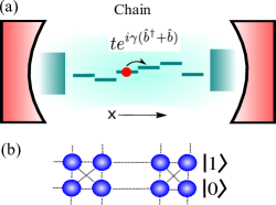
Figure 1: (a) Schematic representation of a chain inside an optical cavity, where the heights indicate the number of photons, and $\gamma$ represents the coupling with the electromagnetic field. (b) As the electron hops, it can absorb or emit a photon, effectively leading to a multi-chain perspective, with $\ket{n}$ denoting the photon state.

II Model and methodology

II.1 The model

The one-dimensional AAH model describes spinless fermions under a quasiperiodic potential Harper (1955); Aubry and André (1980). Its Hamiltonian reads

$$\mathcal{H}_{AA}= -t\sum_{\langle\mathbf{i},\mathbf{j}\rangle}(c^{\dagger}_{\mathbf{i}}c_{\mathbf{j}}^{\phantom{\dagger}}+\text{H.c})$$

$$+g_{AA}\sum_{\mathbf{i}}\cos{(2\pi\beta i+\phi)}c^{\dagger}_{\mathbf{i}}c_{\mathbf{i}}^{\phantom{\dagger}},$$ (1)

where the sums run over a one-dimensional chain, with $\langle\mathbf{i},\mathbf{j}\rangle$ denoting nearest neighbor sites. Here, we use the standard second quantization formalism, in which $c_{\mathbf{i}}^{\dagger}$ ($c_{\mathbf{i}}$) are creation (annihilation) operators of fermions at a given site $\mathbf{i}$. The first term on the right-hand side of Eq. (1) describes the fermionic hopping, while the second term corresponds to the onsite potential, with strenght $g_{AA}$. To describe incommensurate features, one may deal with open boundary conditions (OPC) and define $\beta=\frac{\sqrt{5}-1}{2}$, i.e. as the inverse golden ratio, with $\phi$ being an arbitrary global phase. For periodic boundary conditions (PBC), it is achieved by defining $\beta$ as the ratio of two adjacent Fibonacci numbers, $F_{m-1}/F_{m}$, and extrapolating the results to the thermodynamic limit. Hereafter, the hopping integral, $t$, sets the energy scale and may be taken as unity; similarly, we also take the lattice constant, $a$, as unity.

Interestingly, the Aubry-Andre-Harper model is self-dual, i.e. it is symmetric under a Fourier transform, leading to a sharp transition between extended and localized states: all eigenstates are extended (localized) for $g_{AA}<2$ ($g_{AA}>2$). The model exhibits critical properties only at $g_{AA}=2$, at which the wave function is multifractal Domínguez-Castro and Paredes (2019). Many different extensions of the AAH model have been investigated over the past decades, with the emergence of edge states Biddle et al. (2011); Ganeshan et al. (2015); Liu et al. (2022), as well as for higher dimensions Rossignolo and Dell’Anna (2019). However, examining cavity effects on these extended models is beyond the scope of this work.

As mentioned in the Introduction, we place our one-dimensional AAH electronic system within a cavity with a single-mode electromagnetic field; see Fig. 1. Following Refs. Svintsov et al. (2024) and Li et al. (2020), the coupling between the bosonic and fermionic degrees of freedom changes the hopping integral (Peierls substitution) Peierls (1933), $t\to t\exp[ieaA_{x}/\hbar c\big{]}$, with $A_{x}$ being the vector potential of the electromagnetic field, and $e$ the fermion charge. Here we assume that the wavelength is much larger than the lattice spacing, leading to a position-independent vector potential. Given this, we define $A_{x}=A_{0}(\hat{b}+\hat{b}^{\dagger})$, with $\hat{b}^{\dagger}$ ($\hat{b}$) being creation (annihilation) operators of photons of frequency $\omega_{0}$. The cavity-coupled Hamiltonian then reads,

$$\mathcal{H}= -t\sum_{\langle\mathbf{i},\mathbf{j}\rangle}\bigg{[}e^{i\gamma(\hat{b}+\hat{b}^{\dagger})}c^{\dagger}_{\mathbf{i}}c_{\mathbf{j}}^{\phantom{\dagger}}+\text{H.c}\bigg{]}$$

$$+g_{AA}\sum_{\mathbf{i}}\cos{(2\pi\beta i+\phi)}c^{\dagger}_{\mathbf{i}}c_{\mathbf{i}}^{\phantom{\dagger}}+\hbar\omega_{0}\hat{b}^{\dagger}\hat{b},$$ (2)

where $\gamma=eaA_{0}/(\hbar c)$ describes the coupling with the electromagnetic field, and the last term is the free photons contribution to the energy.

We investigate the Hamiltonian of Eq. (2) through exact diagonalization methods in the subspace of a single fermion coupled to $N_{ph}$ photons. The operators $e^{i\gamma(\hat{b}+\hat{b}^{\dagger})}$ are obtained analytically through the Baker-Campbell-Hausdorff formula (see, e.g., Ref. Svintsov et al. (2024)). In this work, we use both OBC and PBC, while averaging over 10 different random values of $\phi$. We also set a cutoff for the total number of photons at $N_{ph}=8$, which is sufficiently large to ensure that the inclusion of more photon will correspond to weak (negligible) corrections in the inverse participation ratio.

II.2 The inverse participation ratio

A convenient basis for our Hilbert space is spanned by $\ket{l,n}$, with $1\leq l\leq L$ labeling the site position, and $0\leq n\leq N_{ph}$ being the number of photons. We may therefore write a generic (normalized) eigenstate (normalized) of $\mathcal{H}$ as

$$\ket{\psi_{j}}=\sum_{l,n}\phi_{l,n}^{(j)}\ket{l,n},$$ (3)

where $j$ labels the eigenstate, and $\phi_{l,n}^{(j)}$ is the probability amplitude of finding the system in state $\ket{l,n}$.

Given this, one key quantity of interest is the inverse participation ratio (IPR), which determines if a given wavefunction is spatially localized; it is defined as

$$\text{IPR}(\ket{\psi_{j}})=\sum_{l,n}|\phi_{l,n}^{(j)}|^{2q}~{},$$ (4)

with $q=2$. If $\text{IPR}(\ket{\psi_{j}})\to 1$ when $L\to\infty$, the state $\ket{\psi_{j}}$ is localized at a single site. Otherwise $\text{IPR}(\ket{\psi_{j}})\propto 1/N$ so that $\ket{\psi_{j}}$ extends over $N$ sites.

It is more convenient to examine the behavior of the IPR when averaged over a set of $N_{st}$ eigenstates within a specific energy window, $\Delta E=[E_{M_{i}},E_{M_{f}}]$, $M_{i}\leq j\leq M_{f}$,

$$\overline{\text{IPR}}=\frac{1}{N_{st}}\sum_{j=M_{i}}^{M_{f}}\text{IPR}(\ket{\psi_{j}}).$$ (5)

Similarly, and within the same energy window, one may define the minimum IPR, that is

$$\text{IPR}_{min}={\rm min}\big{[}\text{IPR}(\ket{\psi_{j}})\big{]},\forall~{}M_{i}\leq j\leq M_{f}~{}.$$ (6)

While $\overline{\text{IPR}}$ determines the occurrence of localized states for a given set of external parameters, $\text{IPR}_{min}$ establishes the threshold for the occurrence of at least one extended state. Unless otherwise mentioned, in this work we examine both IPR’s for the entire energy spectrum.

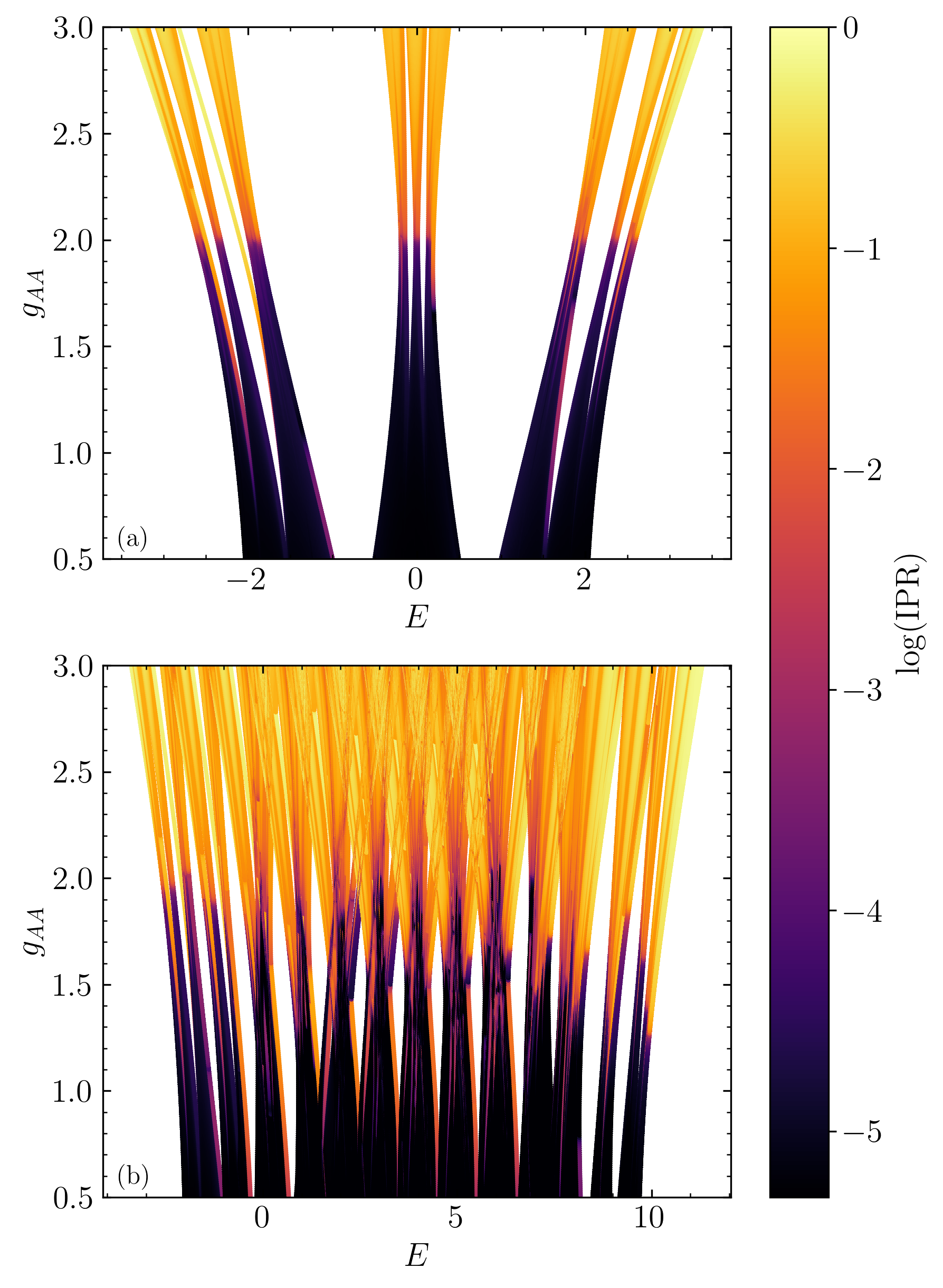
Figure 2: Numerical energy spectrum $E$ as a function of $g_{AA}$ for $L=300$ sites and fixed $\phi=0$. Panel (a) shows the standard AAH model (i.e. no cavity effects), while panel (b) presents the case with coupling with photons. For the latter, we fixed $\omega_{0}=1$ and $\gamma=0.15$, for $N_{ph}=8$ photons. The heatmap describes the IPR associated to each eigenstate, plotted in 10-base logarithmic scale.

II.3 Fractal properties

Another interesting feature of the IPR is its relationship with the fractal dimension of the wavefunction, which indicates how distributed it is within the medium. For extended states, the probability of finding the particle at a given site is proportional to $1/L^{d}$, where $d$ is the dimensionality of the system. This leads to $\text{IPR}\approx L^{d(1-q)}$, which simplifies to $\text{IPR}\approx L^{-d}$ for $q=2$. However, at the critical point, the wavefunction coverage over the medium becomes fractal, rather than homogeneous; accordingly, the scaling properties of the IPR are described through the replacement $d\to D_{f}$, where $D_{f}$ is the fractal dimension.

In the presence of $N_{ph}$ photons, the extension of these ideas is straightforward. Since one expects that $|\phi_{l,n}^{j}|^{2}\approx 1/(L\times N_{ph})^{d}$ for extended states, then $\text{IPR}\approx(L\times N_{ph})^{d(1-q)}$, so that

$$\log(\text{IPR})\approx-D_{f}\big{[}\log(L)+\log(N_{ph})\big{]},$$ (7)

for $q=2$. Therefore, for large, but finite $N_{ph}$, $D_{f}$ may still be extracted from a double-logarithm analysis of the IPR.

Further features of the wave function are provided by performing a multifractal analysis Kohmoto (1983); Liu et al. (2022). Assuming PBC, we choose system sizes from a Fibonacci sequence, $L=F_{m}$. As the probability of finding the particle on a given site $l$ is $P_{l}\propto F_{m}^{-\alpha_{l}^{(j)}}$, the set of exponents $\alpha_{l}^{(j)}$ are used to characterize the distribution of the state $\ket{\psi_{j}}$ over the sites, as follows. We define $\alpha_{min}^{(j)}\equiv\text{min}\big{[}\alpha_{l}^{(j)}\big{]}$, with $1\leq l\leq F_{m}$, and take $m\to\infty$: if $\alpha_{min}^{(j)}\to 1$ or 0, the wave function is extended or localized, respectively; if $0<\alpha_{min}^{(j)}<1$, it is fractal.

Extending these ideas to the present case is also straightforward, with $P_{l}$ obtained by integrating out the photon degrees of freedom, leading to

$$\alpha_{l}^{(j)}=-\frac{\log(\sum_{n}|\phi_{l,n}^{j}|^{2})}{\log(F_{m})}~{}.$$ (8)

Similarly to the IPR case, it is useful to perform a multifractal analysis. With the same definitions as those leading to Eq. (5), we consider the averages

$$\overline{\alpha}_{min}=\frac{1}{N_{st}}\sum_{j=M_{i}}^{M_{f}}\alpha_{min}^{(j)},$$ (9)

which also probe the localized, extended, or fractal character of the wave function, as above.

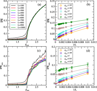
Figure 3: Inverse participation ratio results of the standard AAH model. (a) $\overline{\text{IPR}}$ as a function of $g_{AA}$ for different system sizes $L$. (b) $\overline{\text{IPR}}$ as a function of $1/L$ (symbols) and extrapolated to the thermodynamic limit (solid lines). (c) IPR_min as a function of $g_{AA}$ for different system sizes $L$. (d) IPR_min as a function of $1/L$ (symbols) and extrapolated to the thermodynamic limit (solid lines). Here, and in all subsequent figures, when not shown, error bars are smaller than symbol size.

III Results

We begin our analysis by discussing the established properties of the AAH model without a cavity, which will serve as a baseline when discussing the effects of the coupling with photons. Figure 2 (a) shows the spectrum of the model for different disorder strengths. Notice that all eigenstates change their IPR near $g_{AA}=2$, as demanded by the self-dual property of the model. To probe the critical region it is more convenient to examine the $\overline{\text{IPR}}$ for different system sizes, as shown in Fig. 3 (a). Notice that for $g_{AA}>2$ $\overline{\text{IPR}}$ is large and weakly dependent on the system size, whereas for $g_{AA}<2$ it is small and decreases as $L$ increases. The critical point is obtained by employing a finite-size scaling (FSS) analysis around $g_{AA}=2$, assuming $\overline{\text{IPR}}\propto L^{-D_{f}}$, as presented in Fig. 3 (b), from which one may notice that any $g_{AA}>2$ leads to a finite $\overline{\text{IPR}}$. Similarly, one may check the behavior of $\text{IPR}_{min}$ and its FSS analysis, as shown in Figs. 3 (c), and (d), respectively. One obtains a finite response to $\text{IPR}_{min}$ at $g_{AA}=2$. The former and latter results are consistent with our expectation that in the AAH model all eigenstates become localized at the same critical point. The analysis of the fractal dimension is also consistent with the previous ones, providing $D_{f}=0.53(1)$ at $g_{AA}=2.0$.

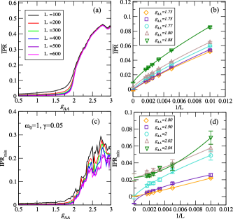
Figure 4: Inverse participation ratio results of the AAH model coupled to the electromagnetic field. Here, we fixed $\gamma=0.05$ and $\omega_{0}=1$. (a) $\overline{\text{IPR}}$ as a function of $g_{AA}$ for different system sizes $L$. (b) $\overline{\text{IPR}}$ as a function of $1/L$ (symbols) and extrapolated to the thermodynamic limit (solid lines). (c) IPR_min as a function of $g_{AA}$ for different system sizes $L$. (d) IPR_min as a function of $1/L$ (symbols) and extrapolated to the thermodynamic limit (solid lines).

We now turn to examine the cavity-coupled case. For instance, Fig. 2 (b) displays the energy spectrum and the IPR behavior for fixed $\omega_{0}=1$ and $\gamma=0.15$, from which differences with respect to the no-cavity case are apparent. First, the electron band is broadened due to the contribution of photons, resulting in an almost continuous spectrum. Second, although we can find extended (localized) states for $g_{AA}\ll 2$ ($g_{AA}\gg 2$), the IPR behavior is quite noisy around $g_{AA}=2$. This noise is enhanced or suppressed if the coupling $\gamma$ with the electromagnetic field is increased or reduced, respectively.

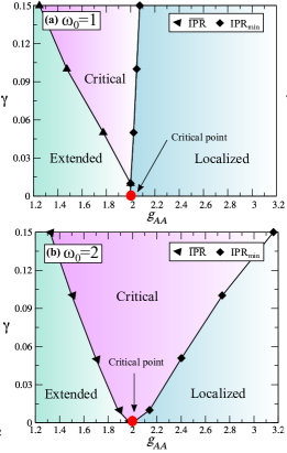
Figure 5: The phase diagram of the AAH model coupled to the electromagnetic field of the optical cavity, where we have integrated over the entire energy spectrum. Here, we fixed (a) $\omega_{0}=1$ and (b) $\omega_{0}=2$. The triangles denote the boundaries given by the $\overline{\text{IPR}}$, while the diamonds represent those provided by the $\text{IPR}_{min}$. The solid lines are just guides to the eye.

In order to further quantify these results, we analyze $\overline{\text{IPR}}$ (over the entire spectrum) for fixed $\omega_{0}=1$ and $\gamma=0.05$, as displayed in Fig. 4 (a); the corresponding FSS analysis is shown in Fig. 4(b). The picture that emerges is that despite being a small coupling, it suffices to displace the edge of the localized phase to $g_{AA}\approx 1.8$. This indicates that the critical point shifts due to the coupling with the cavity, in stark contrast to the standard (cavity-free) case. On the other hand, by examining $\text{IPR}_{min}$ and its FSS analysis, presented in Figs. 4 (c) and (d), respectively, we find a ‘critical’ point at $g_{AA}=2$, consistent with the standard AAH model [see, e.g., Figs. 3 (c) and (d)].

One key observation drawn from the previous results is the following: while $\overline{\text{IPR}}$ represents the average of all IPRs, indicating when a fraction of the states ceases to be extended, $\text{IPR}_{min}$ quantifies the presence of at least one extended state. Thus, the former marks the boundary of the phase in which all eigenstates are extended, while the latter marks the boundary of the phase in which all eigenstates are localized. We recall that in the absence of a cavity, $\overline{\text{IPR}}$ and $\text{IPR}_{min}$ lead to the same critical point; see Fig. 3.

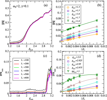
Figure 6: Same as Fig. 4, but for fixed $\gamma=0.1$ and $\omega_{0}=2$.

By repeating the same procedure outlined above for different values of $\gamma$ and fixed $\omega_{0}=1$, we obtain the phase diagram shown in Fig. 5 (a). As discussed below, the intermediate region (i.e., the one with finite $\overline{\text{IPR}}$, but vanishing $\text{IPR}_{min}$) exhibits multifractal features. In view of this, we define this region as critical, although there are some subtleties involving the eigenstates which we discuss below. At any rate, the main effect of the electromagnetic field is to spread the critical point into a critical region, which broadens with increasing coupling.

Let us now discuss how the photon frequency changes the shape of the phase diagram. Figure 6 exhibits the behavior of $\overline{\text{IPR}}$ and $\text{IPR}_{min}$ for fixed $\omega_{0}=2$ and $\gamma=0.1$. While $\overline{\text{IPR}}$ is pushed to smaller values of $g_{AA}$ (similarly to the previous case), $\text{IPR}_{min}$ is pushed to larger values of $g_{AA}$, thus significantly expanding the intermediate region. Analyses for other values of $\gamma$ lead to the phase diagram presented in Fig. 5(b), from which we see that the range of the intermediate region is broader than for $\omega_{0}=1$. At this point, it is worth mentioning that if $\hbar\omega_{0}\gg W$, with $W=4t$ being the bare electron bandwidth, the absorption or emission of photons becomes unlikely, thus decreasing the intermediate region.

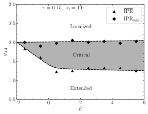
Figure 7: The energy-resolved phase diagram of the AAH model coupled to the electromagnetic field of the optical cavity. Here, we fixed $\omega_{0}=1$ and $\gamma=0.15$. The triangles denote the boundaries given by the $\overline{\text{IPR}}$, while the diamonds represent those provided by the $\text{IPR}_{min}$. The dashed lines are guides to the eye.

At this point, we recall that in certain cases, such as in gate-induced experiments, in which the voltage at the leads – hence the kinetic energy of the electrons – is well-defined. Therefore, we should have at our disposal the extended-localized behavior within specific energy ranges, rather than averaging over the entire spectrum. In view of this, it is worth analyzing $\overline{\text{IPR}}$ and $\text{IPR}_{min}$ at fixed energy ranges. To this end, by generically fixing $\omega_{0}=1$ and $\gamma=0.15$, while varying the energy, $E$ , we determine the critical points for both quantities, as shown in Fig. 7. The behavior for other values of $\gamma$ is similar, differing only by the size of the intermediate region.

There are several key points we should highlight in relation with Fig. 7. First and foremost, one is still able to identify a critical region, although its width depends significantly on the position of the fixed energy interval, being wider for eigenstates with higher energies. Thus, the boundaries in Fig. 5 should be thought of as lower and upper bounds, respectively for $g_{AA}<2$ and $g_{AA}>2$, across the whole energy spectrum. Second, a perturbative treatment of the coupling with the field shows that transitions between states within subspaces with different number of photons are only significant if the unperturbed states are very close in energy. Even though $\gamma=0.15$ leads to nonperturbative effects, the previous argument provides insights into Fig. 7. Specifically, transitions between states in the zero-photon and one-photon subspaces are unlikely for states at the bottom of the energy spectrum, most of which remain in the zero-photon subspace, regardless of the value of $\gamma$. Consequently, for these eigenstates the effect of the coupling is less pronounced, and they are expected to follow the well-known behavior of the standard AAH model. This explains why the intermediate region shrinks to $g_{AA}\approx 2$ as the energy goes to the bottom of the spectrum in Fig. 7. Such behavior should occur for any value of coupling $\gamma$ and photon frequency $\omega_{0}$.

Now we turn to discuss the nature of the electronic states in this intermediate region. It is reasonable to suppose that the coupling with the electromagnetic field would drive the AAH critical point into a critical region. Curiously, a similar qualitative behavior occurs when dealing with spin-orbit coupling, as discussed in Ref. Zhou et al. (2013). Therefore, in order to examine the critical behavior of the eigenstates in the intermediate region, we now perform the multifractal analysis; see Sec. II.3. Here we deal with PBC, considering $L=F_{m}$ as a number of the Fibonacci sequence.

To achieve this goal we start with the analysis of the usual AAH without the cavity coupling, which will serve as a reference when analyzing the effects of coupling with the electromagnetic field. Figure 8(a) displays the behavior of $\overline{\alpha}_{min}(m)$ as a function of $1/m$, for different system sizes, in the absence of photons Their extrapolated values are presented in Fig. 8 (b), where one may notice that, even very close to the critical point (e.g., for $g_{AA}=1.98$ or $2.02$) the extrapolations lead to $\overline{\alpha}_{min}\approx 0$ or 1. Only at $g_{AA}=2$ one obtains an intermediate value of $\overline{\alpha}_{min}$, determining the fractal distribution of the wave function in the medium, and emphasizing that this is the only critical point of the standard AAH model.

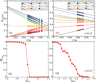
Figure 8: The multifractal analysis for both (a)-(b) the standard AAH model and (c)-(d) the case coupled with the cavity. (a) $\overline{\alpha}_{\min}$(m) as a function of $1/m$ for different values of $g_{AA}$, close to the critical point. The solid lines denote their extrapolation to the thermodynamic limit. (b) The extrapolated results of $\overline{\alpha}_{\min}$ as a function of $g_{AA}$. Panels (c) and (d) are the same as panels (a) and (b), respectively, but for fixed $\gamma=0.15$ and $\omega_{0}=1$, while averaging over the range $\Delta E=[0,2]$.

Given this, we repeat the same procedure to the case with the cavity, whose results are presented in Figs. 8(c) and (d), for fixed $\omega_{0}=1$ and $\gamma=0.15$, and for different values of $g_{AA}$. As the intermediate region depends on the energy range, here we have defined $\Delta E=[0,2]$. Notice that $\overline{\alpha}_{min}\approx 1$ when $g_{AA}\lesssim 1.2$, while $\overline{\alpha}_{min}\approx 0$ when $g_{AA}\gtrsim 2.0$, indicating extended and localized states for these regions, respectively. Indeed, the thresholds provided by $\overline{\alpha}_{min}$ are in good agreement with the critical points identified through the $\overline{\text{IPR}}$ and $\text{IPR}_{min}$ analyses, presented in Fig. 7. Within the intermediate region, $1.2\lesssim g_{AA}\lesssim 2.0$, we obtain a continuous range of values for $\overline{\alpha}_{min}$, which strongly suggests the presence of critical states. That is, differently from the standard AAH model, where such a fractal eigenstate occurs only at the critical point $g_{AA}=2$, the coupling with the photons leads to a critical region.

As $\overline{\alpha}_{min}$ is obtained by averaging over a given energy range, it is also appropriate to examine its probability distribution, rather than the mean value. Figure 9 displays $P\big{[}\alpha_{min}\big{]}$ for $g_{AA}=1.1$, 1.7 and 2.3, with fixed $\omega_{0}=1$, $\gamma=0.15$, and $\Delta E=[0,2]$. Notice that $P\big{[}\alpha_{min}\big{]}$ exhibits a clear and sharp peak at high values of $\alpha_{min}$ for $g_{AA}=1.1$, consistent with extended states. For $g_{AA}=2.3$, the distribution also exhibits a peak, but at low values of $\alpha_{min}$, as expected for localized states. By contrast, fixing $g_{AA}=1.7$ within the intermediate region, we see that $P\big{[}\alpha_{min}\big{]}$ broadens considerably. That is, $P\big{[}\alpha_{min}\big{]}$ changes continuously as a function of $g_{AA}$, reshaping from a peak at large values of $\alpha_{min}$ (for large $g_{AA}$), to a peak at small values of $\alpha_{min}$ (for small $g_{AA}$), through a broad distribution in the intermediate region. This strongly suggests a mixture of extended, localized, and critical states within the intermediate region.

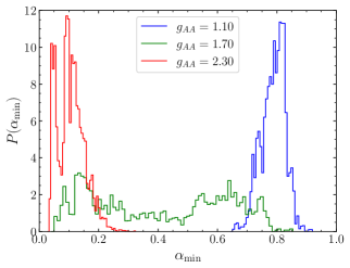
Figure 9: Probability distributions of the multifractal exponent $\alpha_{min}$ of the eigenstates within the energy range $\Delta E=[0,2]$. We fixed $\gamma=0.15$ and $\omega_{0}=1$, and examined $g_{AA}=1.1$ (large peak on the left, shown in red), $g_{AA}=1.7$ (broad distribution in the middle, shown in green), and $g_{AA}=2.3$ (large peak on the right, shown in blue). In all these cases, we examined systems with $L=987$ sites under PBC.

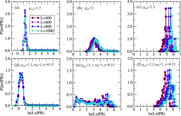
Figure 10: Probability distributions of the logarithm of the IPR as a function of $\ln\big(L\times\text{IPR}\big{missing})$ for different system sizes. Here we examined the $P[\ln({\rm IPR})]$ for the standard AAH model (i.e. without photons) at (a) $g_{AA}=1.7$, (b) $g_{AA}=2.0$, and (c) $g_{AA}=2.3$. Similarly, the $P[\ln({\rm IPR})]$ for the case coupled with the cavity is obtained at (d) $g_{AA}=1.1$, (e) $g_{AA}=1.7$, and (f) $g_{AA}=2.3$, for fixed $\gamma=0.15$ and $\omega_{0}=1$, while averaging over the range $\Delta E=[0,2]$.

Further inspection of the previous findings can be performed by examining the probability distribution of IPR, $P[\ln({\rm IPR})]$. In the extended regime, $L\times\text{IPR}\sim 1$, so that the maximum of the IPR distribution as a function of $\ln\big(L\times\text{IPR}\big{missing})$ should be close to zero and independent of the system size Markos (2006). In the localized regime, where $L\times\text{IPR}\propto L$, $P[\ln({\rm IPR})]$ should peak around $\ln\big(L\big{missing})$, displaying a strong finite-size dependence. This is observed for the standard AAH model, as shown in Figs. 10 (a) and (c) for the extended and localized regimes, respectively. At the critical point of the standard AAH model ($g_{AA}=2$), $P[\ln({\rm IPR})]$ exhibits its maximum for intermediate values of $\ln\big(L\times\text{IPR}\big{missing})$, as presented in Fig. 10 (b). Notice also that $P[\ln({\rm IPR})]$ is weakly dependent on the system size at the critical point, in agreement with the dependence on the fractal dimension, $L\times\text{IPR}\propto L^{(1-D_{f})}$.

Given this, we perform the same analysis for the case with the cavity, fixing $\omega_{0}=1$, $\gamma=0.15$, and $\Delta E=[0,2]$. Figure 10 (d)-(f) shows the behavior of $P[\ln({\rm IPR})]$ for $g_{AA}=1.1$, $1.7$, and $2.3$, respectively. Similarly to the standard AAH model, panels (d) and (f) show the expected behavior for the extended and localized regimes, i.e. with peaks at small and large values of $\ln\big(L\times\text{IPR}\big{missing})$, respectively. However, in the intermediate region (e.g., for $g_{AA}=1.7$) the distribution is broader, as shown in Fig. 10 (e). Interestingly, $P[\ln({\rm IPR})]$ in panel (e) seems to exhibit contributions from size-independent peaks at small $\ln\big(L\times\text{IPR}\big{missing})$, and also from those size-dependent at large values of $\ln\big(L\times\text{IPR}\big{missing})$, while having a continuous distribution in between. This aligns with the behavior of $P\big{[}\alpha_{min}\big{]}$, presented in Fig. 9, thus confirming our claim about the occurrence of a mixture of extended, localized, and critical states at the intermediate region.

IV Conclusions

In this paper we have investigated the effects of a single-mode electromagnetic field coupled to fermionic degrees of freedom of quasiperiodic systems. More specifically, we have focused on how an optical cavity affects the metal-insulator phase transition in quasiperiodic systems. To this end, we have considered fermions described by the one-dimensional Aubry-Andre-Harper model, which exhibits such transition at $g_{AA}=2$ for all eigenstates; this location is exact due to the self-dual property of the model.

We have analyzed the phase transition using both the average and minimum inverse participation ratios, $\overline{\text{IPR}}$ and $\text{IPR}_{\text{min}}$, respectively. While the former determines when a fraction of the states cease to be extended, the latter quantifies the presence of at least one extended state. We have established that, for weak coupling with the electromagnetic cavity, the critical behavior is similar to that for the standard AAH model, with all eigenstates undergoing a phase transition at the same critical point. However, at intermediate or strong coupling, this single critical point broadens into an intermediate region, where $\text{IPR}_{\text{min}}$ vanishes, but $\overline{\text{IPR}}$ remains finite. Further, the size of this intermediate region increases with larger couplings and is strongly dependent on the photon frequency. We have also proposed an energy-resolved phase diagram, which displays the critical points at different energy ranges. As the main result, we observed that the effects of coupling with the cavity are more pronounced at higher energies, with the states at the bottom of the spectrum being hardly affected.

The nature of the intermediate region was examined through a multifractal analysis, by means of the exponent $\alpha_{min}$, which provides a measure of how a given wavefunction spatially spreads through the medium. For the standard AAH model, it shows that the eigenstates are fractal only at the critical point. A similar analysis for the field-coupled case provides evidence of fractal states within the entire intermediate region. We have also investigated the critical properties of the eigenstates by the probability distributions of $\alpha_{min}$ and the IPR. Both distributions are quite broad, strongly suggesting a mixture of extended, localized, and critical states within the intermediate region. That is, the coupling with the electromagnetic field drives the single critical point of the standard AAH model into a critical region. These findings unveil the impact of the coupling of optical cavities on critical transport phenomena and paves the way for further investigations of the influence of cavity-coupling in other metal-insulator transitions. Finally, we hope that the present results may find applications in the design of materials with specific critical transport properties, and in the study of the physics of disordered and quasicrystals structures Krishna Kumar et al. (2018); Xu et al. (2010); Chen et al. (2024).

References

- Ritsch et al. (2013) Helmut Ritsch, Peter Domokos, Ferdinand Brennecke, and Tilman Esslinger, “Cold atoms in cavity-generated dynamical optical potentials,” Rev. Mod. Phys. 85, 553–601 (2013).
- Schlawin et al. (2022) F. Schlawin, D. M. Kennes, and M. A. Sentef, “Cavity quantum materials,” Appl. Phys. Rev. 9, 011312 (2022).
- Léonard et al. (2017) Julian Léonard, Andrea Morales, Philip Zupancic, Tilman Esslinger, and Tobias Donner, “Supersolid formation in a quantum gas breaking a continuous translational symmetry,” Nature 543, 87–90 (2017).
- Léonard et al. (2017) Julian Léonard, Andrea Morales, Philip Zupancic, Tobias Donner, and Tilman Esslinger, “Monitoring and manipulating Higgs and goldstone modes in a supersolid quantum gas,” Science 358, 1415–1418 (2017), https://www.science.org/doi/pdf/10.1126/science.aan2608 .
- Landig et al. (2016) Renate Landig, Lorenz Hruby, Nishant Dogra, Manuele Landini, Rafael Mottl, Tobias Donner, and Tilman Esslinger, “Quantum phases from competing short-and long-range interactions in an optical lattice,” Nature 532, 476–479 (2016).
- Klinder et al. (2015) J. Klinder, H. Keßler, M. Reza Bakhtiari, M. Thorwart, and A. Hemmerich, “Observation of a superradiant mott insulator in the Dicke-Hubbard model,” Phys. Rev. Lett. 115, 230403 (2015).
- Vaidya et al. (2018) Varun D. Vaidya, Yudan Guo, Ronen M. Kroeze, Kyle E. Ballantine, Alicia J. Kollár, Jonathan Keeling, and Benjamin L. Lev, “Tunable-range, photon-mediated atomic interactions in multimode cavity QED,” Phys. Rev. X 8, 011002 (2018).
- Budden et al. (2021) M Budden, T Gebert, M Buzzi, G Jotzu, E Wang, T Matsuyama, G Meier, Y Laplace, D Pontiroli, M Riccò, F. Schlawin, D. Jaksch, and A. Cavalleri, “Evidence for metastable photo-induced superconductivity in k3c60,” Nature Physics 17, 611–618 (2021).
- Sentef et al. (2018) M. A. Sentef, M. Ruggenthaler, and A. Rubio, “Cavity quantum-electrodynamical polaritonically enhanced electron-phonon coupling and its influence on superconductivity,” Science Advances 4, eaau6969 (2018), https://www.science.org/doi/pdf/10.1126/sciadv.aau6969 .
- Schlawin et al. (2019) F. Schlawin, A. Cavalleri, and D. Jaksch, “Cavity-mediated electron-photon superconductivity,” Phys. Rev. Lett. 122, 133602 (2019).
- Curtis et al. (2019) Jonathan B. Curtis, Zachary M. Raines, Andrew A. Allocca, Mohammad Hafezi, and Victor M. Galitski, “Cavity quantum eliashberg enhancement of superconductivity,” Phys. Rev. Lett. 122, 167002 (2019).
- Hartmann et al. (2006) Michael J Hartmann, Fernando GSL Brandao, and Martin B Plenio, “Strongly interacting polaritons in coupled arrays of cavities,” Nature Physics 2, 849–855 (2006).
- Tomadin and Fazio (2010) A. Tomadin and Rosario Fazio, “Many-body phenomena in QED-cavity arrays,” J. Opt. Soc. Am. B 27, A130–A136 (2010).
- Baum et al. (2022) Eli Baum, Amelia Broman, Trevor Clarke, Natanael C. Costa, Jack Mucciaccio, Alexander Yue, Yuxi Zhang, Victoria Norman, Jesse Patton, Marina Radulaski, and Richard T. Scalettar, “Effect of emitters on quantum state transfer in coupled cavity arrays,” Phys. Rev. B 105, 195429 (2022).
- Saxena et al. (2023) Abhi Saxena, Arnab Manna, Rahul Trivedi, and Arka Majumdar, “Realizing tight-binding hamiltonians using site-controlled coupled cavity arrays,” Nature Communications 14, 5260 (2023).
- Patton et al. (2024) JT Patton, Victoria A Norman, Eliana C Mann, Brinda Puri, Richard T Scalettar, and Marina Radulaski, “Polariton creation in coupled cavity arrays with spectrally disordered emitters,” Materials for Quantum Technology 4, 025401 (2024).
- Pisani et al. (2023) F. Pisani, D. Gacemi, and A. et al. Vasanelli, “Electronic transport driven by collective light-matter coupled states in a quantum device,” Nat Commun 14, 3914 (2023).
- Appugliese et al. (2022) F. Appugliese, J. Enkner, G. L. Paravicini-Bagliani, M. Beck, C. Reichl, W. Wegscheider, G. Scalari, C. Ciuti, and J. Faist, “Breakdown of topological protection by cavity vacuum fields in the integer quantum Hall effect,” Science 375, 1030 (2022).
- Orgiu et al. (2015) E. Orgiu, J. George, J. A. Hutchison, E. Devaux, J. F. Dayen, B. Doudin, F. Stellacci, C. Genet, J. Schachenmayer, C. Genes, G. Pupillo, P. Samorì, and T. W. Ebbesen, “Conductivity in organic semiconductors hybridized with the vacuum field,” Nat. Mater. 14, 1123 (2015).
- Hagenmüller et al. (2017) D. Hagenmüller, J. Schachenmayer, S. Schütz, C. Genes, and G. Pupillo, “Cavity-enhanced transport of charge,” Phys. Rev. Lett. 119, 223601 (2017).
- Nataf et al. (2019) P. Nataf, T. Champel, G. Blatter, and D. M. Basko, “Rashba cavity QED: A route towards the superradiant quantum phase transition,” Phys. Rev. Lett. 123, 207402 (2019).
- Guerci et al. (2020) D. Guerci, P. Simon, and C. Mora, “Superradiant phase transition in electronic systems and emergent topological phases,” Phys. Rev. Lett. 125, 257604 (2020).
- Jangjan and Hosseini (2020) Milad Jangjan and Mir Vahid Hosseini, “Floquet engineering of topological metal states and hybridization of edge states with bulk states in dimerized two-leg ladders,” Scientific Reports 10, 14256 (2020).
- Dmytruk and Schirò (2022) Olesia Dmytruk and Marco Schirò, “Controlling topological phases of matter with quantum light,” Communications Physics 5, 271 (2022).
- Allard and Weick (2023) Thomas F. Allard and Guillaume Weick, “Multiple polaritonic edge states in a Su-Schrieffer-Heeger chain strongly coupled to a multimode cavity,” Phys. Rev. B 108, 245417 (2023).
- Ezawa (2024) Motohiko Ezawa, “Topological edge/corner states and polaritons in dimerized/trimerized superconducting qubits in a cavity,” Phys. Rev. B 109, 205421 (2024).
- Liu et al. (2023) Jingyu Liu, Jiani Liu, and Yao Yao, “Parity of polaritons in a molecular aggregate coupled to a single-mode cavity,” Journal of Physics: Condensed Matter 36, 115704 (2023).
- Nguyen et al. (2024) Danh-Phuong Nguyen, Geva Arwas, and Cristiano Ciuti, “Electron conductance of a cavity-embedded topological 1d chain,” arXiv:2402.19244 (2024).
- Bacciconi et al. (2024) Zeno Bacciconi, Gian Marcello Andolina, and Christophe Mora, “Topological protection of Majorana polaritons in a cavity,” Phys. Rev. B 109, 165434 (2024).
- Gómez-León et al. (2024) Álvaro Gómez-León, Marco Schiró’, and Olesia Dmytruk, “High-quality poor man’s Majorana bound states from cavity embedding,” arXiv:2407.12088 (2024).
- Passetti et al. (2023) Giacomo Passetti, Christian J. Eckhardt, Michael A. Sentef, and Dante M. Kennes, “Cavity light-matter entanglement through quantum fluctuations,” Phys. Rev. Lett. 131, 023601 (2023).
- Ashida et al. (2020) Yuto Ashida, Atac Imamoglu, Jerome Faist, Dieter Jaksch, Andrea Cavalleri, and Eugene Demler, “Quantum electrodynamic control of matter: Cavity-enhanced ferroelectric phase transition,” Phys. Rev. X 10, 041027 (2020).
- Masuki and Ashida (2024) Kanta Masuki and Yuto Ashida, “Cavity moiré materials: Controlling magnetic frustration with quantum light-matter interaction,” Phys. Rev. B 109, 195173 (2024).
- Mochida and Ashida (2024) Jun Mochida and Yuto Ashida, “Cavity-enhanced Kondo effect,” Phys. Rev. B 110, 035158 (2024).
- Arwas and Ciuti (2023) Geva Arwas and Cristiano Ciuti, “Quantum electron transport controlled by cavity vacuum fields,” Phys. Rev. B 107, 045425 (2023).
- Svintsov et al. (2024) Dmitry Svintsov, Georgy Alymov, Zhanna Devizorova, and Luis Martin-Moreno, “One-dimensional electron localization in semiconductors coupled to electromagnetic cavities,” Phys. Rev. B 109, 045432 (2024).
- Harper (1955) P G Harper, “Single band motion of conduction electrons in a uniform magnetic field,” Proceedings of the Physical Society. Section A 68, 874 (1955).
- Aubry and André (1980) Serge Aubry and Gilles André, “Analyticity breaking and Anderson localization in incommensurate lattices,” Ann. Israel Phys. Soc 3, 18 (1980).
- Aulbach et al. (2004) Christian Aulbach, Andre Wobst, Gert-Ludwig Ingold, Peter Hänggi, and Imre Varga, “Phase-space visualization of a metal–insulator transition,” New J. Phys. 6, 70 (2004).
- Bu et al. (2022) Xuan Bu, Liang-Jun Zhai, and Shuai Yin, “Quantum criticality in the disordered Aubry-André model,” Phys. Rev. B 106, 214208 (2022).
- Domínguez-Castro and Paredes (2019) G. A. Domínguez-Castro and R. Paredes, “The Aubry–André model as a hobbyhorse for understanding the localization phenomenon,” Eur. J. Phys. 40, 045403 (2019).
- Biddle et al. (2011) J. Biddle, D. J. Priour, B. Wang, and S. Das Sarma, “Localization in one-dimensional lattices with non-nearest-neighbor hopping: Generalized Anderson and Aubry-André models,” Phys. Rev. B 83, 075105 (2011).
- Ganeshan et al. (2015) Sriram Ganeshan, J. H. Pixley, and S. Das Sarma, “Nearest neighbor tight binding models with an exact mobility edge in one dimension,” Phys. Rev. Lett. 114, 146601 (2015).
- Liu et al. (2022) Tong Liu, Xu Xia, Stefano Longhi, and Laurent Sanchez-Palencia, “Anomalous mobility edges in one-dimensional quasiperiodic models,” SciPost Phys. 12, 027 (2022).
- Rossignolo and Dell’Anna (2019) M. Rossignolo and L. Dell’Anna, “Localization transitions and mobility edges in coupled Aubry-André chains,” Phys. Rev. B 99, 054211 (2019).
- Li et al. (2020) Jiajun Li, Denis Golez, Giacomo Mazza, Andrew J. Millis, Antoine Georges, and Martin Eckstein, “Electromagnetic coupling in tight-binding models for strongly correlated light and matter,” Phys. Rev. B 101, 205140 (2020).
- Peierls (1933) Rudolph Peierls, “Zur theorie des diamagnetismus von leitungselektronen,” Zeitschrift für Physik 80, 763–791 (1933).
- Kohmoto (1983) M. Kohmoto, “Metal-insulator transition and scaling for incommensurate systems,” Phys. Rev. Lett. 51, 1198 (1983).
- Note (1) Here we average and over a spectrum width centered at .
- Zhou et al. (2013) Lu Zhou, Han Pu, and Weiping Zhang, “Anderson localization of cold atomic gases with effective spin-orbit interaction in a quasiperiodic optical lattice,” Phys. Rev. A 87, 023625 (2013).
- Note (2) In the present case, since the phase transition of the AAH model occurs at for all eigenstates, we have taken as the whole spectrum, i.e. we average over all eigenstates.
- Markos (2006) Peter Markos, “Numerical analysis of the Anderson localization,” Acta Phys. Slovaca 56, 561–685 (2006).
- Krishna Kumar et al. (2018) R. Krishna Kumar, A. Mishchenko, X. Chen, S. Pezzini, G. H. Auton, D. Ponomarenko, U. Zeitlerc, L. Eaves, and V. I. Falko, “High-order fractal states in graphene superlattices,” PNAS 115, 5135–5139 (2018).
- Xu et al. (2010) Pan Xu, HuiPing Tian, and YueFeng Ji, “One-dimensional fractal photonic crystal and its characteristics,” J. Opt. Soc. Am. B 27, 640–647 (2010).
- Chen et al. (2024) Zhu-Guang Chen, Cunzhong Lou, Kaige Hu, and Lih-King Lim, “Fractal surface states in three-dimensional topological quasicrystals,” (2024), 10.48550/arXiv.2401.11497, arXiv:arXiv:2401.11497 .