Quantum information with quantum-like bits

Abstract

In previous work we have proposed a construction of quantum-like bits that could endow a large, complex classical system, for example of oscillators, with quantum-like function that is not compromised by decoherence. In the present paper we investigate further this platform of quantum-like states. Firstly, we discuss a general protocol on how to construct synchronizing networks that allow for emergent states. We then study how gates can be implemented on those states. This suggests the possibility of quantum-like computing on specially-constructed classical networks. Finally, we define a notion of measurement that allows for non-Kolmogorov interference, a feature that separates our model from a classical probabilistic system. This paper aims to explore the mathematical structure of quantum-like resources, and shows how arbitrary gates can be implemented by manipulating emergent states in those systems.

I Introduction

The present noisy-intermediate scale quantum (NISQ) era of quantum devices is witnessing the successful implementation and test of diverse quantum algorithms on medium-size quantum hardware, from search on unsorted databases, Zhang et al. (2021) to variational quantum algorithms, Cerezo et al. (2021) to simulations of open quantum dynamics. Sun, Shih, and Cheng (2024) However, hardware of at least hundreds of thousands of physical qubits, way beyond the current engineering capabilities, is needed to obtain practical quantum advantage. This involves storing and processing the information volume required by the most challenging and relevant computational problems. Beverland et al. (2022) The critical issue limiting the scalability of quantum resources is the buildup of uncontrolled noise and dissipation, leading to loss of coherence and fidelity. Preskill (2018); Lau et al. (2022); Gill et al. (2022)

In parallel with quantum engineering advancements, ongoing research investigates whether classical computing resources can continue to play a key role in information processing. For example, tensor network simulations have been shown to outperform the most advanced quantum processors in selected algorithms. Tindall et al. (2024) Efficient quantum-inspired protocols have been successfully developed, leveraging advancements in information processing derived from quantum logic. Gharehchopogh (2023)

In the spirit of quantum-inspired computing, we showed in recent work that a large class of synchronizing classical systems can be utilized as a resource for information processing. Scholes (2020, 2023, 2024); Scholes and Amati (2024) The robustness of these systems to noise and stochastic disorder improves with size, following a somehow opposite and favorable trend compared to genuine quantum resources. This well-known behavior is related to the occurrence of classical emergent phenomena and synchronization. Haken (1975); Fano (1992); Strogatz (2012); Artime and De Domenico (2022) Graph theory is the natural mathematical framework used to describe synchronizing many-body systems. Scholes (2020, 2023); Kassabov, Strogatz, and Townsend (2022); Townsend, Stillman, and Strogatz (2020); Rodrigues et al. (2016) In particular, emergent states can be clearly distinguished from a broad band of random states in the spectrum of the adjacency matrices of Erdös-Renyi random graphs and expander families, such as the $k$-regular graphs. Scholes, DelPo, and Kudisch (2020); Scholes (2024); Lubotzky (2012) In Ref. Scholes, 2024, we mapped emergent states onto a computational basis of quantum-like (QL) bits, which can be easily identified from sharp and isolated peaks in the spectra of regular graphs. This feature implies that QL states are easily distinguishable and measurable even in presence of noise and dissipation, that can usually broaden the spectral lines of the network. In Ref. Scholes and Amati, 2024 we built on these results and proposed a general structure for the resources of multiple QL bits, based on the Cartesian products of one-QL-bit graphs.

Our approach is derived consistently with a QL probabilistic framework proposed by Khrennikov. Khrennikov (2007a, 2019, 2010) This theory shows that genuine quantum systems are not strictly required to process information in a QL way. Instead, to observe QL phenomena it is sufficient to construct a contextual probability theory involving suitable notions of QL states, observables, and their measurement.

In the present paper we extend the foundational work of Ref. Scholes, 2024; Scholes and Amati, 2024; Scholes, 2023 to formalize the notion of QL states and gates. Furthermore, consistently with Khrennikov’s approach, Khrennikov (2010) we list a set of measurement axioms which allows to define a generalized notion of nonclassical interference between observable operators.

The present paper is structured as follows. In ?? we summarize the formalism describing how to construct a single-QL-bit Hilbert space. In ?? we discuss its generalization to higher dimensions, and we show explicitly in ?? how to construct Bell states for two QL bits. In ?? we study the action of a complete set of QL gates, and we provide concrete examples of their action. Finally, in ??, we present a set of axioms that enables us to define a QL probabilistic theory in our approach. In particular, we highlight the presence of a nonclassical interference term in the relation between total and conditional probabilities, specific to non-Kolmogorovian contextual probabilistic models. Khrennikov (2010)

In conjunction with Refs. Scholes, 2023; Scholes and Amati, 2024; Scholes, 2024, this work provides the mathematical foundation for a rigorous approach to QL information processing from classical synchronizing systems.

II Quantum-like bits

In this section we derive a mapping a from classical network to the Hilbert space of interacting QL bits. While the concept has been already elucidated in Ref. Scholes, 2024, here we lay out a more formal description. Later in the paper we use this formalism to study the notion of gates to perform quantum information processing, and we provide concrete examples.

II.1 Isolated system

Let us consider two classical many-body systems with pairwise interactions between the elementary constituents. Those systems can be mapped onto two graphs $G_{1}$ and $G_{2}$. We assume here that both graphs involve the same number of vertices ${N_{G}}$, and we label by $A_{1}$ and $A_{2}$ the related adjacency matrices. For simplicity we focus here on undirected simple graphs, without loops. The adjacency matrix for this class of graphs is symmetric with entries either $0$ or $1$ and null diagonal. Additionally, we assume an isotropic structure for all two-body interactions, such that the valence of the graphs is constant and equal to $k$. Diestel (2017) In particular,

$$\sum_{i=1}^{N_{G}}[A_{n}]_{ij^{\prime}}=\sum_{j=1}^{N_{G}}[A_{n}]_{i^{\prime}j}=k,\hskip 22.76219pt\forall i^{\prime},j^{\prime}=1,\cdots,{N_{G}},$$ (II.1)

where $n=1,2$. We highlight that, as proven in recent work, Scholes (2023); Scholes and Amati (2024) the present formalism is robust even in the presence of disorder in the network, which may violate the condition of exact regularity. Consequently, the theory discussed in the paper is also applicable to quasi-regular resources, provided analytical results on matrix algebra are replaced by their more general numerical analogs. The direct sum of the two adjacency matrices is

$$A_{1}\oplus A_{2}=\begin{bmatrix}A_{1}&\mathbb{0}_{N_{G}}\\ \mathbb{0}_{N_{G}}&A_{2}\end{bmatrix},$$ (II.2)

where we labeled by $\mathbb{0}_{N_{G}}\in M_{N_{G}}(\mathbb{N})$ the null matrix on the off-diagonal blocks. As proposed in Ref. Scholes, 2024, to define QL bits we switch on an interaction between the two subgraphs, and define the resource

$$\mathcal{R}=\begin{bmatrix}A_{1}&C\\ C^{\top}&A_{2}\end{bmatrix},$$ (II.3)

involving a coupling matrix $C$. Note that $C$ does not represent a simple graph by itself, i.e. it is in general non-symmetric, and it can admit diagonal entries mapping corresponding vertices in $A_{1}$ and $A_{2}$. Conversely, ??, being overall symmetric and loop-free, describes a simple undirected graph. We sample $C$ by randomly assigning $1$ to $N_{\mathrm{C}}\leq{N_{G}}^{2}$ of its entries. This matrix is chosen to be regular with valency $l=N_{\mathrm{C}}/{N_{G}}$ [similarly to ??]. ?? represents the fundamental resource used to build an isolated QL bit. Scholes (2024)

To better describe the structure of the graphs that are suitable resources for our QL platform, we show in ?? four instances of ?? for increasing values of $l$, as specified in the captions.

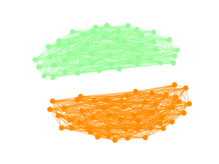
$l=0$

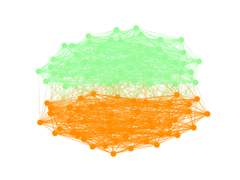
$l=k/4$

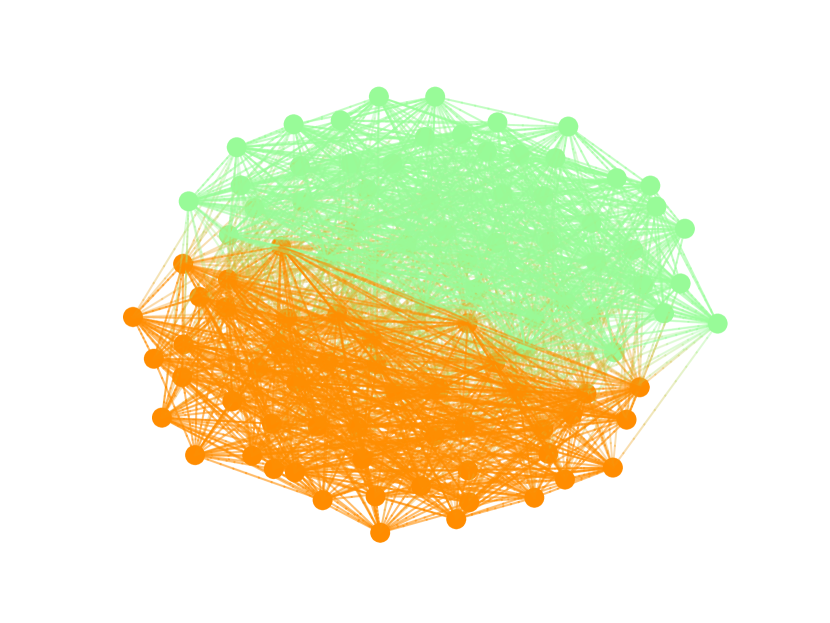
$l=k/2$

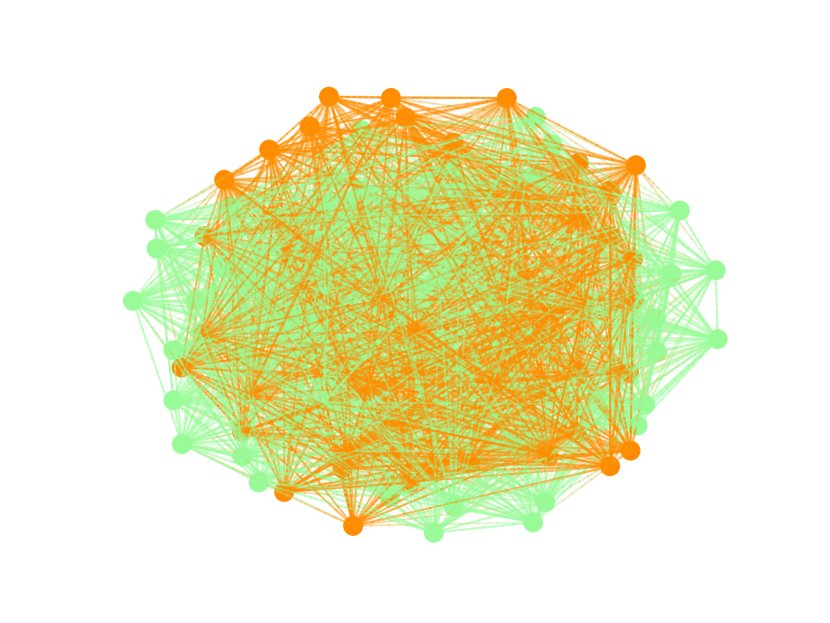
$l=k$

Figure 1: Graphs associated to the resource ??, for increasing values of the valency $l$ of the coupling matrix $C$, as specified in the captions. $l$ is given here in units of the valency $k$ of the subgraphs $A_{1}$ (light green/light) and $A_{2}$ (dark orange/dark). The other parameters are fixed to ${N_{G}}=50$ and $k=20$.

The case $l=0$ corresponds to uncoupled regular graphs, as in ??. By increasing $l$, we strengthen the coupling between the two subgraphs. For $l=k$, ?? turns into a regular matrix with total valency $2k$, with the same density of both intra- and cross- subgraphs edges.

As discussed in Refs. Scholes, 2023, 2024, resources with structure as in ?? are particularly appealing for information processing. In fact, these resources allow for emergent states associated to distinguishable eigenvalues, well isolated from a large band of random states. By mapping the states associated to those peaks onto a Hilbert space, we obtain a platform for information logic that can be controlled by network manipulation. We will elaborate on this important concept further in the manuscript.

We study the spectral properties of the resources by plotting in ?? the distribution $\rho(\lambda)$ of the eigenvalues of ?? for increasing values of the valency $l$ of $C$.

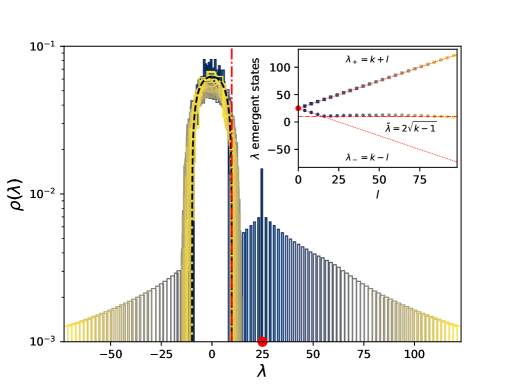
Figure 2: Main panel: distribution of the eigenvalues $\lambda$ of the QL-resource ??, for increasing values of the order $l$ of the coupling matrix $C$, from $l=0$ (blue/dark) to $l={N_{G}}$ (yellow/light). Inset: largest and second largest eigenvalues of the spectrum as a function of $l$, with the same color code as in the main panel. We fix here ${N_{G}}=100$ and $k=25$.

Results are shown from $l=0$ (blue/dark) to $l={N_{G}}$ (yellow/light). The other parameters are fixed to ${N_{G}}=100$ and $k=25$. The emergent states can be identified for each $l$ from the isolated sharp peaks in the spectrum. For $l=0$ we observe a single isolated line associated to the two-fold degenerate eigenvalue $\lambda=k=25$ (red markers). As the valency $l$ increases, this emergent eigenvalue split into two, and the peaks shift to $\lambda_{\pm}=k\pm l$. We track the “ballistic” evolutions of the eigenvectors as a function of the coupling valency $l$ in the inset of ??. Here, the largest and second largest eigenvalues are shown as squared and dotted markers, respectively. While the value of the largest eigenvalue increases linearly for arbitrary $l$, we observe that the second largest eigenvalue plateaus at values close to $\tilde{\lambda}=2\sqrt{k-1}$. This barrier is defined by the radius of the Wigner semicircle distribution for a graph of order $k$, shown as a black dashed line in the figure. McKay (1981); Farkas et al. (2001) This portion of the spectrum is populated by random low-frequency states, whose high density makes them hardly distinguishable. Scholes (2020, 2023, 2024) From the present analysis we infer that, by fixing $l=(k-\tilde{\lambda})/2$, both the distance between the two emergent eigenvalues and between those and the dark states are maximized. As elucidated in Ref. Scholes, 2023, 2024, this analysis offers valuable insight for creating well-resolved and easily distinguishable emergent states for quantum information purposes.

We discuss now how to construct the Hilbert space $\mathcal{H}^{(1)}$ of an isolated QL qubit from coupled regular graphs, with adjacency matrices with structure as in ??. In particular, we define the mapping

$$\psi_{+}=\tfrac{1}{\sqrt{2}}\begin{pmatrix}a_{1}\\ a_{2}\end{pmatrix}\mapsto\ket{+},\hskip 17.07164pt\psi_{-}=\tfrac{1}{\sqrt{2}}\begin{pmatrix}a_{1}\\ -a_{2}\end{pmatrix}\mapsto\ket{-},$$ (II.4)

where $a_{i}$ is the normalized eigenvector associated to the largest eigenvalue of $A_{i}$. The vectors $\psi_{\sigma}$, $\sigma\in\{+,-\}$, are eigenvectors of ?? with eigenvalues $k\pm l$. In the following we show that the mapping in ?? leads to a well-defined Hilbert space. First of all, it is straightforward to show that the $\psi_{\sigma}$’s are mutually orthogonal and normalized:

$$\braket{\psi_{\sigma},\psi_{\sigma^{\prime}}} =\sum_{i=1}^{2{N_{G}}}\psi_{\sigma,i}^{*}\psi_{\sigma^{\prime},i}=\frac{1}{2}\left(|a_{1}|^{2}+(2\delta_{\sigma\sigma^{\prime}}-1)|a_{2}|^{2}\right)$$

$$=\delta_{\sigma\sigma^{\prime}}\mapsto\braket{{\sigma}{\sigma^{\prime}}}{,}$$ (II.5)

where $\sigma,\sigma^{\prime}\in\{+,-\}\equiv\mathcal{S}$. Operators acting on ?? are expressed in terms of the matrices in $M_{2{N_{G}}}(\mathbb{R})$

$$\Psi_{\sigma\sigma^{\prime}}=\psi_{\sigma}\otimes\psi_{\sigma^{\prime}}^{\dagger}\mapsto\ket{\sigma}\bra{\sigma^{\prime}}.$$ (II.6)

As it would be expected in an abstract Hilbert space, the maps in ?? combine according to the rule

$$\Psi_{\sigma\sigma^{\prime}}\Psi_{\pi\pi^{\prime}}=\Psi_{\sigma\pi^{\prime}}\braket{\psi_{\sigma^{\prime}},\psi_{\pi}},$$ (II.7)

and they transform under Hermitian conjugation as $\Psi_{\sigma\sigma^{\prime}}^{\dagger}=\Psi_{\sigma^{\prime}\sigma}$.

In this section we summarized a list of prescriptions for defining a mapping from a bipartite graph to the Hilbert space of a single qubit, and related properties. Scholes and Amati (2024); Scholes (2024) In the next ?? we expand on an idea proposed in Ref. Scholes and Amati, 2024, to represent entanglement and superposition by coupling together multiple graph resources. Formal derivations on how to implement information processing and define a QL probabilistic model in this framework, follow in the later ????, respectively.

II.2 Many-body system

II.2.1 Formalism

Various representations of the quantum states are possible with respect to classical network structures. For a small number of QL bits the representation defined in Ref. Scholes, 2024 is useful. In that work the Bell states, involving two QL bits, are designed to give insight on proof-of-principle examples of entanglement. In Ref. Scholes and Amati, 2024 we propose a formal representation of states applicable to an arbitrary number of QL bits. This is based on the Cartesian product of single-QL-bit graphs. Consistently with that work, we define here as a simple generalization of ?? the resource for a system of ${N_{\mathrm{QL}}}$ bits

$$\mathcal{R}=\sum_{q=1}^{N_{\mathrm{QL}}}\left[\bigotimes_{p=1}^{q-1}\mathbb{1}_{2{N_{G}}}\right]\otimes\mathcal{R}^{(q)}\otimes\left[\bigotimes_{p^{\prime}=q+1}^{{N_{\mathrm{QL}}}}\mathbb{1}_{2{N_{G}}}\right],$$ (II.8)

where each $\mathcal{R}^{(q)}$ has the structure shown in ??. The tensors

$$\psi_{\bm{\sigma}}=\bigotimes_{q=1}^{{N_{\mathrm{QL}}}}\psi_{\sigma^{(q)}}\mapsto\bigotimes_{q=1}^{{N_{\mathrm{QL}}}}\ket{\sigma^{(q)}}=\ket{\bm{\sigma}},$$ (II.9)

are eigenvectors of ??. Here, different basis elements are labeled using the multi-index $\bm{\sigma}=\left\{\sigma^{(1)},\cdots,\sigma^{(N_{\mathrm{QL}})}\right\}$, while the components of ?? are expressed via the multi-index $\bm{i}=\left\{i^{(1)},\cdots,i^{(N_{\mathrm{QL}})}\right\}$ as

$$[\psi_{\bm{\sigma}}]_{\bm{i}} =\prod_{q=1}^{N_{\mathrm{QL}}}\psi_{\sigma^{(q)},i^{(q)}}.$$ (II.10)

As discussed after ??, each $\psi_{\sigma^{(q)}}$, with $\sigma^{(q)}\in\{+,-\}$, is associated to one of the eigenvalues $k\pm l$ of $\mathcal{R}^{(q)}$. Let us label this eigenvalue $\lambda_{\sigma^{(q)}}$. The action of $\mathcal{R}$ on $\psi_{\bm{\sigma}}$ is then given by

$$\mathcal{R}\psi_{\bm{\sigma}} =\sum_{q=1}^{N_{\mathrm{QL}}}\left[\bigotimes_{p=1}^{q-1}\psi_{\sigma^{(p)}}\right]\otimes\left[\mathcal{R}^{(q)}\psi_{\sigma^{(q)}}\right]\otimes\left[\bigotimes_{p^{\prime}=q+1}^{{N_{\mathrm{QL}}}}\psi_{\sigma^{(p^{\prime})}}\right]$$

$$=\sum_{q=1}^{N_{\mathrm{QL}}}\lambda_{\sigma^{(q)}}^{(q)}\psi_{\bm{\sigma}}=\lambda_{\bm{\sigma}}\psi_{\bm{\sigma}},$$ (II.11)

where

$$\lambda_{\bm{\sigma}}=\sum_{q=1}^{N_{\mathrm{QL}}}\lambda_{\sigma^{(q)}}^{(q)}.$$ (II.12)

???? tell us that the spectrum of the resource $\mathcal{R}$ of ${N_{\mathrm{QL}}}$ QL bits will involve peaks corresponding to sums of the emergent eigenvalues of each $\mathcal{R}^{(q)}$. Scholes and Amati (2024)

In analogy to ?? for ${N_{\mathrm{QL}}}=1$, the states in ?? define an orthonormal basis for $\mathcal{H}$ according to the scalar product defined by

$$\braket{\psi_{\bm{\sigma}},\psi_{\bm{\sigma}^{\prime}}} =\frac{1}{2^{N_{\mathrm{QL}}}}\prod_{q=1}^{{N_{\mathrm{QL}}}}\left[|a_{1}^{(q)}|^{2}+(2\delta_{\sigma^{(q)},\sigma^{\prime(q)}}-1)|a_{2}^{(q)}|^{2}\right]$$

$$=\prod_{q=1}^{{N_{\mathrm{QL}}}}\delta_{{\sigma}^{(q)},{\sigma^{\prime}}^{(q)}}=\prod_{q=1}^{{N_{\mathrm{QL}}}}\braket{\sigma^{(q)}}{{\sigma^{\prime}}^{(q)}}.$$ (II.13)

Similarly, we extend the mapping of operators in ?? to

$$\Psi_{\bm{\sigma},\bm{\sigma}^{\prime}} =\psi_{\bm{\sigma}}\otimes\psi_{\bm{\sigma}^{\prime}}^{\dagger}\mapsto\bigotimes_{q=1}^{{N_{\mathrm{QL}}}}\ket{{\sigma}_{q}^{(q)}}\bra{{\sigma^{\prime}}_{q}^{(q)}}=\ket{\bm{\sigma}}\bra{\bm{\sigma}^{\prime}},$$ (II.14)

with components

$$\left[\Psi_{\bm{\sigma},\bm{\sigma}^{\prime}}\right]_{\bm{i,j}}=\prod_{q=1}^{N_{\mathrm{QL}}}\psi_{\sigma^{(q)},i^{(q)}}\psi^{*}_{\sigma^{\prime(q)},j^{(q)}}.$$ (II.15)

The Hermitian conjugate of ?? is defined such that

$$\left[\Psi_{\bm{\sigma},\bm{\sigma}^{\prime}}^{\dagger}\right]_{\bm{ij}}=\prod_{q=1}^{N_{\mathrm{QL}}}\psi_{\sigma^{(q)},j^{(q)}}^{*}\psi_{\sigma^{\prime(q)},i^{(q)}}=\left[\Psi_{\bm{\sigma}^{\prime},\bm{\sigma}}\right]_{\bm{ij}},$$ (II.16)

and we generalize ?? to

$$\Psi_{\bm{\sigma\sigma^{\prime}}}\Psi_{\bm{\pi\pi^{\prime}}}=\Psi_{\bm{\sigma\pi^{\prime}}}\braket{\bm{\psi_{\sigma^{\prime}}},\bm{\psi_{\pi}}}.$$ (II.17)

The mapping discussed here provides a general description of state vectors, entanglement and operators constructed from the emergent states of an arbitrary number of QL bits. In the next ?? we show explicitly, as an example, how to construct maximally entangled Bell states for ${N_{\mathrm{QL}}}=2$.

II.2.2 Example: Bell states

Here, we study the spectral properties of two-QL-bit resources, and we show how to construct entangled Bell states with them. ?? in this case simplifies to

$$\mathcal{R}=\mathcal{R}^{(1)}\otimes\mathbb{1}_{2{N_{G}}}+\mathbb{1}_{2{N_{G}}}\otimes\mathcal{R}^{(2)}.$$ (II.18)

The spectrum $\rho(\lambda)$ of a resource with structure as in ?? is shown in ?? for the system parameters ${N_{G}}=16$, $k=6$ and $l=1$. To improve the smoothness of all distributions, we average over a number of $N_{\mathrm{samp}}=10^{3}$ realizations of random regular graphs. The black curve corresponds to the direct (dir.) calculation from the eigenvalues of ??. An alternative approach to calculate the spectrum is possible, by observing that each eigenvalue $\lambda_{i}$ of ?? can be expressed as a sum $\lambda_{i}=\lambda^{(1)}_{j}+\lambda^{(2)}_{k}$, where the $\lambda^{(q)}_{m}$’s are eigenvalues of $\mathcal{R}^{(q)}$, $q=1,2$.Scholes and Amati (2024) We can therefore calculate the spectrum of ?? via the convolution

$$\rho(\lambda)=\int_{-\infty}^{+\infty}\mathrm{d}x\;\rho^{(1)}(x)\rho^{(2)}(\lambda-x),$$ (II.19)

where $\rho^{(q)}(x)$ is the spectrum of a single QL bit, analogously to what shown in ??. The generalization of ?? provides a simple recipe to construct the spectrum of a system of an arbitrary number of QL bits starting from the spectra for ${N_{\mathrm{QL}}}=1$. The distribution calculated from the convolution (conv.) ??, is shown as a green (light) dashed curve in ??, and it agrees satisfactorily with the direct calculation. We mark in red on the picture the isolated peaks corresponding to the emergent eigenvalues of the two-QL-bit systems. These are $\lambda_{++}=2k+2l$ (circle), $\lambda_{+-}=\lambda_{-+}=2k$ (cross) and $\lambda_{--}=2k-2l$ (square). These eigenvalues are associated to the corresponding eigenvectors $\{\psi_{\sigma\sigma^{\prime}}\}_{\sigma,\sigma^{\prime}\in\mathcal{S}}$, defining an orthonormal basis for the Hilbert space of two QL bits.

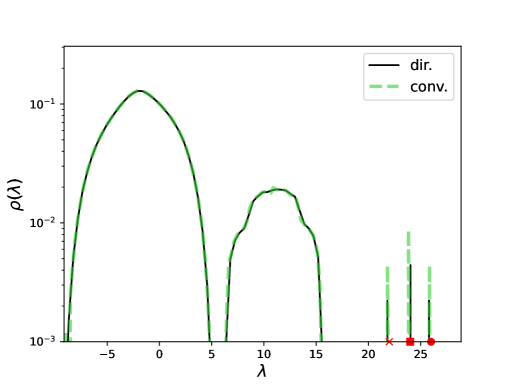
Figure 3: Distribution of the eigenvalues of ??, for $N_{\mathrm{s}amp}=10^{3}$ random samples of the graphs resources. The parameters of the graph are fixed here to ${N_{G}}=16$, $k=6$, $l=1$. The solid black curve corresponds to the direct sampling of the eigenvalues of ??, while the green dashed curve is obtained from the convolution of two identical one-QL-bit distributions [??].

To obtain the explicit expression of the eigenvectors, it is convenient to label the eigenvectors of each QL bit as

$$\psi^{(1)}_{\pm}=\begin{pmatrix}a_{1}\\ \pm a_{2}\end{pmatrix},\hskip 14.22636pt\psi^{(2)}_{\pm}=\begin{pmatrix}b_{1}\\ \pm b_{2}\end{pmatrix},$$ (II.20)

where $a_{i}$’s and $b_{i}$’s are defined as in ?? for the resources ${\mathcal{R}}^{(1)}$ and ${\mathcal{R}}^{(2)}$, respectively. With ?? we can express

$$\psi_{+\pm} =\frac{1}{2}\begin{pmatrix}a_{1}\otimes b_{1}&\pm a_{1}\otimes b_{2}\\ a_{2}\otimes b_{1}&\pm a_{2}\otimes b_{2}\end{pmatrix},$$ (II.21a)

$$\psi_{-\pm} =\frac{1}{2}\begin{pmatrix}a_{1}\otimes b_{1}&\pm a_{1}\otimes b_{2}\\ -a_{2}\otimes b_{1}&\mp a_{2}\otimes b_{2}\end{pmatrix}.$$ (II.21b)

We can finally construct maximally entangled Bell states via the linear combinations

$$\Phi^{\mathrm{Bell}}_{\pm} =\tfrac{1}{\sqrt{2}}\left(\psi_{++}\pm\psi_{--}\right),$$ (II.22a)

$$\Psi^{\mathrm{Bell}}_{\pm} =\tfrac{1}{\sqrt{2}}\left(\psi_{+-}\pm\psi_{-+}\right),$$ (II.22b)

that is,

$$\Phi^{\mathrm{Bell}}_{+} =\frac{1}{\sqrt{2}}\begin{pmatrix}a_{1}\otimes b_{1}&\mathbb{0}_{N}\\ \mathbb{0}_{N}&a_{2}\otimes b_{2}\end{pmatrix},$$ (II.23a)

$$\Phi^{\mathrm{Bell}}_{-} =\frac{1}{\sqrt{2}}\begin{pmatrix}\mathbb{0}_{N}&a_{1}\otimes b_{2}\\ a_{2}\otimes b_{1}&\mathbb{0}_{N}\end{pmatrix},$$ (II.23b)

$$\Psi^{\mathrm{Bell}}_{+} =\frac{1}{\sqrt{2}}\begin{pmatrix}a_{1}\otimes b_{1}&\mathbb{0}_{N}\\ \mathbb{0}_{N}&-a_{2}\otimes b_{2}\end{pmatrix},$$ (II.23c)

$$\Psi^{\mathrm{Bell}}_{-} =\frac{1}{\sqrt{2}}\begin{pmatrix}\mathbb{0}_{N}&-a_{1}\otimes b_{2}\\ a_{2}\otimes b_{1}&\mathbb{0}_{N}\end{pmatrix}.$$ (II.23d)

By applying the mapping from emergent states to the Hilbert space of QL bits, as discussed here, we can introduce the concept of QL gates for information processing. We propose an approach to implement these gates in the next ??.

III Quantum-like gates

In this section, we discuss the fundamental principles of QL information processing. Specifically, we demonstrate how the emergent states of QL resources can be transformed consistently to any arbitrary quantum gate. We then outline a perspectives on how to translate these transformations onto operations on the edges of the graph resources. This is particularly relevant for the future computational and experimental implementation of QL algorithms.

To connect the usual definition of gates acting on an abstract Hilbert space to our QL formalism, it is convenient to introduce a map $U_{\mathrm{cb}}$ transforming the emergent eigenvectors onto the standard factorized computational basis. This map is defined by

$$U_{\mathrm{cb}}=[V_{\mathrm{H}}\otimes\mathbb{1}_{N_{G}}]^{\otimes{N_{\mathrm{QL}}}},$$ (III.1)

where

$$V_{\mathrm{H}}=\frac{1}{\sqrt{2}}\begin{pmatrix}1&1\\ 1&-1\end{pmatrix}$$ (III.2)

denotes the standard Hadamard (H) gate. ?? acts on the factorized states as

$$U_{\mathrm{cb}}\psi_{\bm{\sigma}} =\bigotimes_{q=1}^{{N_{\mathrm{QL}}}}\begin{pmatrix}\frac{1}{2}[1+\sigma^{(q)}]1_{N_{G}}\\ \frac{1}{2}[1-\sigma^{(q)}]1_{N_{G}}\end{pmatrix},$$ (III.3)

where

$$x_{M}=(x,\cdots,x)/\sqrt{M}\in\mathbb{C}^{M},\hskip 28.45274ptx\in\mathbb{C},\;M\in\mathbb{N}.$$ (III.4)

The action of $U_{\mathrm{cb}}$ becomes clear for ${N_{\mathrm{QL}}}=1$, where

$$U_{\mathrm{cb}}\psi_{+}=\begin{pmatrix}1_{N_{G}}\\ 0_{N_{G}}\end{pmatrix},\hskip 14.22636ptU_{\mathrm{cb}}\psi_{-}=\begin{pmatrix}0_{N_{G}}\\ 1_{N_{G}}\end{pmatrix}.$$ (III.5)

We show in ?? how to construct the transformation $U_{\mathrm{cb}}$ in the more general case of non-regular graphs. The QL analog of any arbitrary quantum gate $V_{\mathrm{g}}$ is defined by the matrix transformation

$$U_{\mathrm{g}}=U_{\mathrm{cb}}^{-1}(V_{\mathrm{g}}\otimes\mathbb{1}_{{N_{G}}})U_{\mathrm{cb}}.$$ (III.6)

Let us consider a few examples of ??. The QL maps of the identity operator and the three Pauli gates are, in the limit of exactly regular graphs,

$$U_{\mathcal{I}} =\begin{pmatrix}\mathbb{1}_{N_{G}}&\mathbb{0}_{N_{G}}\\ \mathbb{0}_{N_{G}}&\mathbb{1}_{N_{G}}\end{pmatrix},$$ (III.7a)

$$U_{X} =\begin{pmatrix}\mathbb{1}_{N_{G}}&\mathbb{0}_{N_{G}}\\ \mathbb{0}_{N_{G}}&-\mathbb{1}_{N_{G}}\end{pmatrix},$$ (III.7b)

$$U_{\mathrm{Y}} =\begin{pmatrix}\mathbb{0}_{N_{G}}&i\mathbb{1}_{N_{G}}\\ -i\mathbb{1}_{N_{G}}&\mathbb{0}_{N_{G}}\end{pmatrix},$$ (III.7c)

$$U_{\mathrm{Z}} =\begin{pmatrix}\mathbb{0}_{N_{G}}&\mathbb{1}_{N_{G}}\\ \mathbb{1}_{N_{G}}&\mathbb{0}_{N_{G}}\end{pmatrix},$$ (III.7d)

respectively. As expected, the transformations in ?? act as the standard Pauli gates:

$$U_{\mathrm{X}}\psi_{\pm}=\psi_{\mp},\hskip 14.22636ptU_{\mathrm{Y}}\psi_{\pm}=\pm i\psi_{\mp},\hskip 14.22636ptU_{\mathrm{Z}}\psi_{\pm}=\pm\psi_{\pm}.$$ (III.8)

As another example, the QL map of the Hadamard gate entangles the states of the factorized basis:

$$U_{\mathrm{H}}\psi_{\pm}=\left(V_{\mathrm{H}}\otimes\mathbb{1}_{{N_{G}}}\right)\psi_{\pm}=\frac{1}{\sqrt{2}}(\psi_{+}\pm\psi_{-}).$$ (III.9)

Finally, the two-QL-bit controlled NOT (CN) gate acts on the second QL bit as either the identity or the NOT gate, depending on the control state defined by the first QL bit. It is defined in an abstract Hilbert space by $\hat{V}_{\mathrm{CN}}=\ket{+}\bra{+}\otimes\hat{\mathcal{I}}+\ket{-}\bra{-}\otimes\hat{\mathrm{X}}$, where $\hat{\mathcal{I}}$ and $\hat{\mathrm{X}}$ are the identity and the Pauli-X operator, respectively. Its QL representation is

$$U_{\mathrm{CN}} =\frac{1}{2}(U_{\mathcal{I}}+U_{\mathrm{Z}})\otimes U_{\mathcal{I}}+\frac{1}{2}(U_{\mathcal{I}}-U_{\mathrm{Z}})\otimes U_{\mathrm{X}},$$ (III.10)

transforming elements of the factorized basis as follows:

$$U_{\mathrm{CN}}\psi_{+\pm}=\psi_{+\pm},\hskip 28.45274ptU_{\mathrm{CN}}\psi_{-\pm}=\psi_{-\mp}.$$ (III.11)

Up to this point, we have focused exclusively on the action of QL gates on states $\psi_{\bm{\sigma}}$ of the factorized basis. We can infer from those the transformation of any arbitrary state $\psi=\sum_{\bm{\sigma}\in\bm{\mathcal{S}}}\gamma_{\bm{\sigma}}\psi_{\bm{\sigma}}$, $\gamma_{\bm{\sigma}}\in\mathbb{C}$, thanks to linearity of the map ??. In future work, we aim to design a bijective map $\psi\mapsto\mathcal{R}_{\psi}$ between QL states and resources. This approach enables the mapping of any gate transformation on states, $\psi\mapsto U_{\mathrm{g}}\psi=\psi_{\mathrm{g}}$, onto operations on cluster of edges of the corresponding resources, $\mathcal{R}_{\psi}\mapsto\mathcal{R}_{\psi_{\mathrm{g}}}$. This provides a clear numerical and experimental framework for QL computing.

In the next ?? we shift the discussion towards the benefits provided by a suitable measure theory designed to add “quantumness” to an otherwise classical network. This framework fulfills premises which can be key for a future quantification of QL advantage, as originally proposed in Ref. Khrennikov, 2019.

IV Quantum-like measurements

In this section, we discuss criteria that allows to introduce a notion of QL interference of probabilities in our approach. This highlights that genuine quantum mechanical systems are not strictly required to build QL stochastic models provided the notions of states, observables and measurement are defined according to a given set of prescriptions.

IV.1 Axiomatic definition

In the following we present a list of axioms, originally proposed in Ref. Khrennikov, 2010, to equip our classical network resources with a stochastic theory which mirrors the probability laws of genuine quantum mechanical systems.

Axiom 1.

QL states are represented by normalized vectors in a Hilbert space $\mathcal{H}$.

States can be expressed by linear combinations of elements of the factorized basis ??:

$$\psi=\sum_{\bm{\sigma}\in\bm{\mathcal{S}}}\alpha_{\bm{\sigma}}\psi_{\bm{\sigma}},$$ (IV.1)

Pure QL states are by definition normalized, and we establish the equivalence class $\beta\psi\sim\psi$ for $\beta\in\mathbb{C}$, $|\beta|=1$.

Axiom 2.

QL observables are represented by self-adjointed operators on $\mathcal{H}$. Their action on QL states, expressed by linear maps, defines a QL measurement.

Observables are expressed in term of linear combinations with structure

$$\mathcal{F} =\sum_{{\bm{\sigma},\bm{\sigma}^{\prime}\in\bm{\mathcal{S}}}}\left(\gamma_{\bm{\sigma},\bm{\sigma}^{\prime}}\Psi_{\bm{\sigma},\bm{\sigma}^{\prime}}+\gamma^{*}_{\bm{\sigma},\bm{\sigma}^{\prime}}\Psi_{\bm{\sigma}^{\prime},\bm{\sigma}}\right),\hskip 14.22636pt\gamma_{\bm{\sigma},\bm{\sigma}^{\prime}}\in\mathbb{C},$$ (IV.2)

and fulfill the self-adjointness condition $\mathcal{F}^{\dagger}=\mathcal{F}$, as defined in ??. The QL measurement of $\mathcal{F}$ on a state $\psi$ is defined by the map $\psi\mapsto\mathcal{F}\psi$.

Axiom 3.

The spectrum of a QL observable is a measurable quantity.

An arbitrary observable $\mathcal{F}$, as defined in ??, is diagonalizable. Its normalized eigenvectors $\{f_{\bm{\sigma}}\}$_σ∈S define an orthonormal basis of $\mathcal{H}$, while the corresponding eigenvalues are real and distinct. Proofs of these standard properties for the specific structure of our QL Hilbert space are given in ??.

Axiom 4.

A QL probability measure defined by Born’s rule is assigned to the spectrum of physical observables.

Specifically, let us consider a generic state $\psi\in\mathcal{H}$. We define by

$$P_{\psi}\left(\lambda_{\bm{\sigma}}^{\mathcal{F}}\right)=\left\lVert\Pi^{\mathcal{F}}_{\bm{\sigma}}\psi\right\rVert^{2}=|\braket{f_{\bm{\sigma}},\psi}|^{2},$$ (IV.3)

the QL probability of collapsing onto the subspace spanned by the eigenvector $f_{\bm{\sigma}}$, with eigenvalue $\lambda^{\mathcal{F}}_{\bm{\sigma}}$, after measuring $\mathcal{F}$ on $\psi$. ?? is expressed in terms of the projector

$$\Pi^{\mathcal{F}}_{\bm{\sigma}}=f_{\bm{\sigma}}\otimes f_{\bm{\sigma}}^{\dagger}=\left(\Pi^{\mathcal{F}}_{\bm{\sigma}}\right)^{2}.$$ (IV.4)

Axiom 5.

QL conditional probabilities are defined via consecutive projections onto the eigenstates of physical observables.

In particular, let us consider two generic QL observable operators $\mathcal{F}$ and $\mathcal{G}$ whose spectra are defined by

$$\mathcal{F}f_{\bm{\sigma}}=\lambda_{\bm{\sigma}}^{\mathcal{F}}f_{\bm{\sigma}},\hskip 28.45274pt\mathcal{G}g_{\bm{\sigma}}=\lambda_{\bm{\sigma}}^{\mathcal{G}}g_{\bm{\sigma}}.$$ (IV.5)

For a nonzero state $\psi$ we denote by

$$P_{\psi}\left(\lambda^{\mathcal{G}}_{\bm{\sigma}^{\prime}}|\lambda^{\mathcal{F}}_{\bm{\sigma}}\right)=\frac{\left\lVert\Pi^{\mathcal{G}}_{\bm{\sigma}^{\prime}}\Pi^{\mathcal{F}}_{\bm{\sigma}}\psi\right\rVert^{2}}{\left\lVert\Pi^{\mathcal{F}}_{\bm{\sigma}}\psi\right\rVert^{2}}$$ (IV.6)

the QL conditional probabilities associated to the consecutive measures of $\mathcal{F}$ and $\mathcal{G}$ on a state $\psi$.

We show in the next ?? that the QL probability model defined via Axioms 1 to 5 violates by construction Kolmogorovian classical statistics. This feature allows to introduce a notion of QL interference in our approach. Khrennikov (2003, 2019)

IV.2 Quantum probabilities in a QL model

Before introducing a formula for the update of QL probabilities, it is instructive to briefly recall its classical correspondent, to assess analogies and differences between the two. A classical probability space is defined by the triplet $\{\Omega,\Sigma,P^{(\mathrm{cl})}\}$, where $\Omega$ is a space of experimental outcomes, $\Sigma$ the $\sigma$-algebra of its subsets, and $P^{(\mathrm{cl})}$ a probability measure on $\Sigma$.Shiryaev and Wilson (2013) Be $\{\mathcal{A}_{j}\}_{j=1}^{J}$ a partition of $\Omega$, i.e. a collection of $J$ sets defined such that $A_{j}\neq\emptyset\;\forall j$, $\mathcal{A}_{j}\cap A_{j^{\prime}}=\emptyset$ for $j\neq j^{\prime}$ and $\cup_{j=1}^{J}\mathcal{A}_{j}=\Omega$. $P^{(\mathrm{cl})}$ is a positive measure on the partition elements, that is $P^{(\mathrm{cl})}(\mathcal{A}_{j})>0\;\forall j$, and it is normalized: $\sum_{j=1}^{J}P^{(\mathrm{cl})}(\mathcal{A}_{j})=1$. For every $\mathcal{B}\in\Sigma$ the classical formula of total probabilities holds: Kolmogoroff (1933)

$$P^{(\mathrm{cl})}(\mathcal{B}) =P^{(\mathrm{cl})}\left(\mathcal{B}\cap\cup_{j=1}^{J}A_{j}\right)$$

$$=\sum_{j=1}^{J}P^{(\mathrm{cl})}\left(\mathcal{B}\cap A_{j}\right)=\sum_{j=1}^{J}P^{(\mathrm{cl})}(\mathcal{B}|\mathcal{A}_{j})P^{(\mathrm{cl})}(\mathcal{A}_{j}),$$ (IV.7)

where we introduced the classical conditional probability

$$P^{(\mathrm{cl})}(\mathcal{B}|\mathcal{A}_{j})=\frac{P^{(\mathrm{cl})}(\mathcal{B}\cap\mathcal{A}_{j})}{P^{(\mathrm{cl})}(\mathcal{A}_{j})}.$$ (IV.8)

We discuss now the correspondent of ?? for the present QL framework. Let $\mathcal{F}$ and $\mathcal{G}$ be two nondegenerate QL observbles, whose eigenvalue problems are defined as in ??. In this case, the QL conditional probabilities defined in ?? lose their dependence on the initial state $\psi$:

$$P_{\psi}\left(\lambda^{\mathcal{G}}_{\bm{\sigma}^{\prime}}|\lambda^{\mathcal{F}}_{\bm{\sigma}}\right) \mapsto|\braket{g_{\bm{\sigma}^{\prime}},f_{\bm{\sigma}}}|^{2}\equiv P\left(\lambda^{\mathcal{G}}_{\bm{\sigma}^{\prime}}|\lambda^{\mathcal{F}}_{\bm{\sigma}}\right).$$ (IV.9)

Note that the probabilities in ?? are symmetric, differently from their classical correspondents in ??. Observables $\mathcal{F}$ and $\mathcal{G}$ obeying this property for all $\bm{\sigma},\bm{\sigma}^{\prime}\in\bm{\mathcal{S}}$ are called symmetrically conditioned. Khrennikov (2010) This feature is a signature of Bohr’s principle of contextuality, Bohr (1987); Khrennikov and Kozyrev (2005); Khrennikov (2022) expressing the impossibility of strictly separating physical observables and the experimental context under which those are measured. The role of contextuality in a QL probabilitistic framework can be highlighted by rewriting total and conditional probabilities [????, respectively], on an equal footing:

$$P\left(\lambda^{\mathcal{G}}_{\bm{\sigma}}|\lambda^{\mathcal{F}}_{\bm{\sigma}^{\prime}}\right)=\left.P_{\psi}(\lambda^{\mathcal{G}}_{\bm{\sigma}})\right|_{\psi=f_{\bm{\sigma}^{\prime}}}.$$ (IV.10)

If ?? is fulfilled, Axioms 1 to 5 lead to the QL formula for probability updates Khrennikov (2007b, 2010); Bulinski and Khrennikov (2004)

$$P_{\psi}\left(\lambda_{\bm{\sigma}}^{\mathcal{G}}\right) =\sum_{\bm{\sigma}^{\prime}\in\bm{\mathcal{S}}}P_{\psi}\left(\lambda_{\bm{\sigma}^{\prime}}^{\mathcal{F}}\right)P\left(\lambda^{\mathcal{F}}_{\bm{\sigma}^{\prime}}|\lambda^{\mathcal{G}}_{\bm{\sigma}}\right)$$

$$\quad+\sum_{\begin{subarray}{c}\bm{\sigma}^{\prime},\bm{\sigma}^{\prime\prime}\in\bm{\mathcal{S}}\\ \bm{\sigma}^{\prime}\neq\bm{\sigma}^{\prime\prime}\end{subarray}}\Lambda^{\psi}_{\bm{\sigma},\bm{\sigma}^{\prime},\bm{\sigma}^{\prime\prime}}\Big{[}P_{\psi}\left(\lambda_{\bm{\sigma}^{\prime}}^{\mathcal{F}}\right)P\left(\lambda^{\mathcal{F}}_{\bm{\sigma}^{\prime}}|\lambda^{\mathcal{G}}_{\bm{\sigma}}\right)$$

$$\quad\times P_{\psi}\left(\lambda_{\bm{\sigma}^{\prime\prime}}^{\mathcal{F}}\right)P\left(\lambda^{\mathcal{F}}_{\bm{\sigma}^{\prime\prime}}|\lambda^{\mathcal{G}}_{\bm{\sigma}}\right)\Big{]}^{1/2}.$$ (IV.11)

An extended derivation of ?? is provided in ??, where we give the explicit expression of the nonclassical interference coefficient $\Lambda^{\psi}_{\bm{\sigma},\bm{\sigma}^{\prime},\bm{\sigma}^{\prime\prime}}$ [??]. Information processing can be designed in a QL way, to enhance or suppress some spectral measurements compared to classical computing protocols. Khrennikov (2021)
As discussed in Ref. Khrennikov, 2021, an important feature of the QL probability formula ?? is that it does not require the calculation of exponentially time-consuming joint probability distributions. Instead, these are necessary for the classical updates described by ??. This observation is connected to the foundation of quantum advantage. We aim to explore this relevant property in future test of QL algorithms.

V Conclusions

In this paper, we expanded upon the general approach derived in Refs. Scholes, 2023, 2024; Scholes and Amati, 2024 to define and manipulate QL states. In ?? we constructed a computational basis from the emergent states of many-body classical systems, whose correlations can be mapped onto synchronizing graphs. We introduced the Hilbert space for an arbitrary number of QL bits, and we derived explicitly the Bell states in dimension two. We then proposed in ?? a notion of quantum gates applicable to QL states, and we provided concrete examples of their action. Finally, we discussed in ?? a list of measurement axioms which allow to observe QL interference effects in our approach.

Several open questions remain, presenting diverse opportunities for future research.

In the paper we introduced notions of entanglement, interference, and QL probabilities which avoid the expensive calculation of joint distributions. In future work we plan to investigate how each of these features contributes to achieving a “QL advantage” over strictly classical information processing. The ultimate test of the approach proposed in this work will be to implement benchmark algorithms, and evaluate their time efficiency and resource cost. Bharti et al. (2022)

In the last decades, advanced error correction techniques have been developed to minimize loss of information and decoherence in quantum processors. Cai et al. (2023); Campbell (2024) Similarly, we can ask how to prevent and minimize errors in our framework, e.g. in presence of impurities and irregularities in the structure of the graphs. In this regard, we note that a foundational property of synchronizing graphs is that their robustness against uncontrolled noise and dissipation increases with size. Scholes (2023); Scholes and Amati (2024); Anwar et al. (2023) Therefore, we conjecture that error correction is achievable in our approach by simply increasing the number of classical nodes of the graphs. We aim to further explore this concept in future work, to provide bounds of fidelity of gate transformations as a function of the size of the system and strength of external noise.

It can be insightful to directly relate our work to the rigorous approach to quantum non-Markovianity proposed in Refs. Pollock et al., 2018a; White et al., 2020; Berk et al., 2023. In that framework a notion of conditional probabilities is defined, that accounts explicitly for the role of measurement devices on the statistics. An important feature of that formalism is that it provides an operational definition of non-Markovianity which, differently from other strategies, converges to the correct Kolmogorov conditions in the classical limit. Pollock et al. (2018b)

A broad class of computational approaches to open quantum systems and quantum chemistry involves a perspective somehow complementary to our approach. In particular, quantum nonadiabatic systems are often mapped onto quasiclassical models to minimize computational complexity and inexpensively approximate long-time dynamics. Accurate quasiclassical methods have been derived, by requiring that Kolmogorov probabilities [fulfilling ??] obey by construction quantum detailed balance at long times. Amati, Mannouch, and Richardson (2023); Amati, Runeson, and Richardson (2023); Runeson et al. (2022); Amati et al. (2022); Mannouch and Richardson (2023) It can be insightful to assess whether even more accurate quasiclassical approaches can be derived from a QL stochastic theory which approximates ?? beyond the first classical term.

From an experimental standpoint, different options can be explored to implement synchronizing resources for QL information processing. Insulator-to-metal-transition devices and spin-torque oscillators are viable candidates, as they allow for both distributed and parallel computing, while ensuring good robustness to noise and fault tolerance. Raychowdhury et al. (2019) In future work, we aim to further analyze platforms to experimentally implement QL resources, and the properties required by different approaches for optimal network implementation and manipulation.

The environmental implications of the large-scale industrial production of quantum processors are topics of ongoing debate. Ezratty (2023); Ikonen, Salmilehto, and Möttönen (2017); Paler and Basmadjian (2022) For instance, superconducting devices require significant energy due to the cryogenic cooling of the constituent superconducting circuits. Similarly, quantum computers based on arrays of Rydberg atoms demand intensive energy resources. Meyer (2000); Bernien et al. (2017) Implementing energy-efficient classical circuits for QL computing can contribute to sustainable quantum-processing engineering. Additionally, our method leverages classical synchronization, which scales more efficiently with resources compared to its quantum-mechanical counterpart. Aifer, Thingna, and Deffner (2024)

Finally, it can be a fascinating topic for future research to connect QL information processing introduced here to other information theories on human decision-making and psychology derived in the framework of contextual probability models. This idea has been extensively discussed in the literature of QL probabilistic models.Khrennikov (2016); Ozawa and Khrennikov (2020); Scholes (2024); Widdows, Rani, and Pothos (2023) Implementing our formalism on brain-like neuromorphic circuits Pal et al. (2024) can foster theoretical and experimental investigations in this framework.

VI Acknowledgments

This research was funded by the National Science Foundation under Grant No. 2211326 and the Gordon and Betty Moore Foundation through Grant GBMF7114.

Appendix A Transformation of the emergent states to the computational basis

In ?? we discussed how a QL representation of quantum gates can be straightforwardly defined once the emergent states are mapped onto the computational basis. In general, this transformation cannot be expressed in analytic form as soon as the subgraphs defining the resources are not exactly regular. However, we show here that the problem of determining the map can be rewritten as a matrix inversion problem, easily solvable with standard numeric algebra tools.

Firstly, it is convenient to parametrize the generalization of ?? as follows:

$$U_{\mathrm{cb}}=\bigotimes_{q=1}^{N_{\mathrm{QL}}}\begin{pmatrix}X^{(q)}&Y^{(q)}\\ W^{(q)}&Z^{(q)}\end{pmatrix},$$ (A.1)

where $X^{(q)}\in\mathbb{R}^{{N_{G}}}$ is diagonal, with components $X_{ij}^{(q)}=\delta_{ij}x_{j}^{(q)}$, and similarly for the other three blocks in ??. ?? can be rewritten as the linear problem

$$x_{i}^{(q)}a_{1,i}^{(q)}+y_{i}^{(q)}a_{2,i}^{(q)} ={N_{G}}^{-1/2},$$ (A.2a)

$$w_{i}^{(q)}a_{1,i}^{(q)}+z_{i}^{(q)}a_{2,i}^{(q)} =0,$$ (A.2b)

$$x_{i}^{(q)}a_{1,i}^{(q)}-y_{i}^{(q)}a_{2,i}^{(q)} =0,$$ (A.2c)

$$w_{i}^{(q)}a_{1,i}^{(q)}-z_{i}^{(q)}a_{2,i}^{(q)} ={N_{G}}^{-1/2},$$ (A.2d)

where $q=1,\cdots,{N_{\mathrm{QL}}}$, $i=1,\cdots,{N_{G}}$, and where we made use of the generalization of ?? to arbitrary values of ${N_{\mathrm{QL}}}$:

$$\psi_{\pm}^{(q)}=\tfrac{1}{\sqrt{2}}\begin{pmatrix}a_{1}^{(q)}\\ a_{2}^{(q)}\end{pmatrix}.$$ (A.3)

?? is expressed in matrix form as

$$\begin{pmatrix}D_{1}^{(q)}&D_{2}^{(q)}&\mathbb{0}_{N_{G}}&\mathbb{0}_{N_{G}}\\ \mathbb{0}_{N_{G}}&\mathbb{0}_{N_{G}}&D_{1}^{(q)}&D_{2}^{(q)}\\ D_{1}^{(q)}&-D_{2}^{(q)}&\mathbb{0}_{N_{G}}&\mathbb{0}_{N_{G}}\\ \mathbb{0}_{N_{G}}&\mathbb{0}_{N_{G}}&D_{1}^{(q)}&-D_{2}^{(q)}\end{pmatrix}\begin{pmatrix}x^{(q)}\\ y^{(q)}\\ w^{(q)}\\ z^{(q)}\end{pmatrix}=\begin{pmatrix}1_{N_{G}}\\ 0_{N_{G}}\\ 0_{N_{G}}\\ 1_{N_{G}}\end{pmatrix},$$ (A.4)

where $\left[D_{n}^{(q)}\right]_{ij}=\delta_{ij}a_{n,j}^{(q)}$, $n=1,2$. ?? can be inverted to determine a solution for $\left(x^{(q)},y^{(q)},w^{(q)},z^{(q)}\right)$ $\forall q=1,\cdots{N_{\mathrm{QL}}}$, corresponding to a unique expression for $U_{\mathrm{cb}}$.

Appendix B Derivation of the quantum-like formula of total probabilities

In this appendix we derive ??, describing the update of probabilities for two QL observables $\mathcal{F}$ and $\mathcal{G}$, with eigenvalue problems defined as in ??.

Any state vector $\psi\in\mathcal{H}$ can be expanded as

$$\psi=\sum_{\bm{\sigma}\in\bm{\mathcal{S}}}G^{\psi}_{\bm{\sigma}}g_{\bm{\sigma}}=\sum_{\bm{\sigma}^{\prime}\in\bm{\mathcal{S}}}F^{\psi}_{\bm{\sigma}^{\prime}}f_{\bm{\sigma}^{\prime}},$$ (B.1)

where $F^{\psi}_{\bm{\sigma}^{\prime}}=\braket{f_{\bm{\sigma}^{\prime}},\psi}$ and $G^{\psi}_{\bm{\sigma}}=\braket{g_{\bm{\sigma}},\psi}$. We can connect the probabilities of the two observables by expressing

$$\psi =\sum_{\bm{\sigma},\bm{\sigma}^{\prime}\in\bm{\mathcal{S}}}F^{\psi}_{\bm{\sigma}^{\prime}}u_{\bm{\sigma}^{\prime},\bm{\sigma}}g_{\bm{\sigma}},$$ (B.2a)

$$u_{\bm{\sigma}^{\prime},\bm{\sigma}} =\braket{g_{\bm{\sigma}},f_{\bm{\sigma}^{\prime}}}.$$ (B.2b)

which leads to the following mapping between the coefficients of $\psi$ in the two bases:

$$G^{\psi}_{\bm{\sigma}}=\sum_{\bm{\sigma}^{\prime}\in\bm{\mathcal{S}}}F^{\psi}_{\bm{\sigma}^{\prime}}u_{\bm{\sigma}^{\prime},\bm{\sigma}}.$$ (B.3)

To relate ?? to QL probabilities, we define

$$F^{\psi}_{\bm{\sigma}^{\prime}}=\,\mathrm{e}^{i\gamma_{\bm{\sigma}^{\prime}}^{\psi}}\sqrt{P_{\psi}\left(\lambda_{\bm{\sigma}^{\prime}}^{\mathcal{F}}\right)},\hskip 11.38109ptu_{\bm{\sigma}^{\prime},\bm{\sigma}}=\,\mathrm{e}^{i\Gamma_{\bm{\sigma}^{\prime},\bm{\sigma}}}\sqrt{P\left(\lambda^{\mathcal{F}}_{\bm{\sigma}^{\prime}}|\lambda^{\mathcal{G}}_{\bm{\sigma}}\right)},$$ (B.4)

where $\gamma^{\psi}_{\bm{\sigma}^{\prime}},\Gamma_{\bm{\sigma}^{\prime},\bm{\sigma}}\in[0,2\pi)$. By expanding the squared modulus of ??, we finally obtain ??. This involves the phase factor

$$\Lambda^{\psi}_{\bm{\sigma},\bm{\sigma}^{\prime},\bm{\sigma}^{\prime\prime}}=\,\mathrm{e}^{i\left(\gamma^{\psi}_{\bm{\sigma}^{\prime}}-\gamma^{\psi}_{\bm{\sigma}^{\prime\prime}}\right)}\,\mathrm{e}^{i\left(\Gamma_{\bm{\sigma}^{\prime},\bm{\sigma}}-\Gamma_{\bm{\sigma}^{\prime\prime},\bm{\sigma}}\right)},$$ (B.5)

which, being any other term of ?? real, can be replaced by its real part:

$$\Lambda^{\psi}_{\bm{\sigma},\bm{\sigma}^{\prime},\bm{\sigma}^{\prime\prime}}\mapsto\cos\left[(\gamma^{\psi}_{\bm{\sigma}^{\prime}}-\gamma^{\psi}_{\bm{\sigma}^{\prime\prime}})(\Gamma_{\bm{\sigma}^{\prime},\bm{\sigma}}-\Gamma_{\bm{\sigma}^{\prime\prime},\bm{\sigma}})\right].$$ (B.6)

Appendix C Spectral properties of QL observables

In this appendix we study the spectral properties of QL observables [??], that are Hermitian operators according to the definition ??. In particular, we show that (i) their eigenvalues are real, (ii) eigenvectors corresponding to different eigenvalues are orthogonal, and (iii) there exists an orthonormal basis of $\mathcal{H}$ consisting of eigenvectors. We refer here to the eigenvalues and eigenvectors of $\mathcal{F}$ as $\lambda_{\bm{\sigma}}$’s and $f_{\bm{\sigma}}$’s, respectively.

1. For an arbitrary $f_{\bm{\sigma}}$

   $$\braket{f_{\bm{\sigma}},\mathcal{F}f_{\bm{\sigma}}}=\lambda_{\bm{\sigma}}\left\lVert f_{\bm{\sigma}}\right\rVert^{2}=\braket{\mathcal{F}f_{\bm{\sigma}},f_{\bm{\sigma}}}=\lambda_{\bm{\sigma}}^{*}\left\lVert f_{\bm{\sigma}}\right\rVert^{2},$$

   which implies that $\lambda_{\bm{\sigma}}\in\mathbb{R}$.

2. Suppose that $\lambda_{\bm{\sigma}}\neq\lambda_{\bm{\sigma}^{\prime}}$ for $\bm{\sigma}\neq\bm{\sigma}^{\prime}$. By multiplying

   $$\mathcal{F}f_{\bm{\sigma}}=\lambda_{\bm{\sigma}}f_{\bm{\sigma}},$$ (C.1)

   by $f_{\bm{\sigma}^{\prime}}$, we obtain

   $$\langle f_{\bm{\sigma}^{\prime}},\mathcal{F}f_{\bm{\sigma}}\rangle =\lambda_{\bm{\sigma}}\langle f_{\bm{\sigma}^{\prime}},f_{\bm{\sigma}}\rangle$$

   $$=\langle\mathcal{F}f_{\bm{\sigma}^{\prime}},f_{\bm{\sigma}}\rangle\begin{subarray}{c}\ref{enum:i}\\ =\end{subarray}\lambda_{\bm{\sigma}^{\prime}}\langle f_{\bm{\sigma}^{\prime}},f_{\bm{\sigma}}\rangle,$$ (C.2)

   which implies that $\langle f_{\bm{\sigma}^{\prime}},f_{\bm{\sigma}}\rangle=0$.

3. Let us order the eigenvalues and eigenvectors of $\mathcal{F}$ in increasing order, via the map

   $$\bm{\sigma}\mapsto n=\sum_{q=1}^{N_{\mathrm{QL}}}2^{{N_{\mathrm{QL}}}-q}\left(\frac{1-\sigma^{(q)}}{2}\right)+1.$$ (C.3)

   Let us define by $V_{1}$ the set of vectors orthogonal to the eigenvector $f_{1}$ of $\mathcal{F}$ with eigenvalue $\lambda_{1}$. Note that $\mathcal{F}$ maps $V_{1}$ onto itself, i.e., $\mathcal{F}\psi\in V_{1}$ for $\psi\in V_{1}$. In fact,

   $$\braket{f_{1},\mathcal{F}\psi}=\braket{\mathcal{F}f_{1},\psi}=\lambda_{1}\braket{f_{1},\psi}=0.$$ (C.4)

   The linear operator $L(\phi)=\mathcal{F}\phi$, when restricted to $V_{1}$, is also Hermitian, and it admits an eigenvalue $\lambda_{2}$ with eigenvector $f_{2}\in V_{1}$. By construction, $f_{2}$ is orthogonal to $f_{1}$. We then define by $V_{2}$ the orthogonal complement to $\mathrm{span}\{f_{1},f_{2}\}$. Again, $\mathcal{F}$ maps $V_{2}$ onto itself. By proceeding this way, we find a sequence $\{\lambda_{n},f_{n},V_{n}\}_{n}$, where the subspace $V_{n}$ is orthogonal to $\mathrm{span}\{f_{1},\cdots,f_{n}\}$. The sequence ends at the step of order $2^{N_{\mathrm{QL}}}$, given that $\dim(V_{n})=2^{N_{\mathrm{QL}}}-n$. This process allows us to define a complete set of mutually orthogonal eigenvectors.

References

- Zhang et al. (2021) K. Zhang, P. Rao, K. Yu, H. Lim, and V. Korepin, “Implementation of efficient quantum search algorithms on NISQ computers,” Quantum Inf. Process. 20, 233 (2021).
- Cerezo et al. (2021) M. Cerezo, A. Arrasmith, R. Babbush, S. C. Benjamin, S. Endo, K. Fujii, J. R. McClean, K. Mitarai, X. Yuan, L. Cincio, and P. J. Coles, “Variational quantum algorithms,” Nat. Rev. Phys. 3, 625–644 (2021).
- Sun, Shih, and Cheng (2024) S. Sun, L.-C. Shih, and Y.-C. Cheng, “Efficient quantum simulation of open quantum system dynamics on noisy quantum computers,” Phys. Scr. 99, 035101 (2024).
- Beverland et al. (2022) M. E. Beverland, P. Murali, M. Troyer, K. M. Svore, T. Hoefler, V. Kliuchnikov, G. H. Low, M. Soeken, A. Sundaram, and A. Vaschillo, “Assessing requirements to scale to practical quantum advantage,” arXiv:2211.07629 (2022).
- Preskill (2018) J. Preskill, “Quantum Computing in the NISQ era and beyond,” Quantum 2, 79 (2018).
- Lau et al. (2022) J. W. Z. Lau, K. H. Lim, H. Shrotriya, and L. C. Kwek, “NISQ computing: where are we and where do we go?” AAPPS Bullet. 32, 27 (2022).
- Gill et al. (2022) S. S. Gill, A. Kumar, H. Singh, M. Singh, K. Kaur, M. Usman, and R. Buyya, “Quantum computing: A taxonomy, systematic review and future directions,” Softw. - Pract. Exp. 52, 66–114 (2022).
- Tindall et al. (2024) J. Tindall, M. Fishman, E. M. Stoudenmire, and D. Sels, “Efficient Tensor Network Simulation of IBM’s Eagle Kicked Ising Experiment,” PRX Quantum 5, 010308 (2024).
- Gharehchopogh (2023) F. S. Gharehchopogh, “Quantum-inspired metaheuristic algorithms: comprehensive survey and classification,” Artif. Intell. Rev. 56, 5479–5543 (2023).
- Scholes (2020) G. D. Scholes, “Polaritons and excitons: Hamiltonian design for enhanced coherence,” Proc. R. Soc. A: Math. Phys. Eng. Sci. 476, 20200278 (2020).
- Scholes (2023) G. D. Scholes, “Large Coherent States Formed from Disordered k-Regular Random Graphs,” Entropy 25, 1519 (2023).
- Scholes (2024) G. D. Scholes, “Quantum-like states on complex synchronized networks,” Proc. R. Soc. A: Math. Phys. Eng. Sci. 480, 20240209 (2024).
- Scholes and Amati (2024) G. D. Scholes and G. Amati, “Quantum-like product states constructed from classical networks,” arXiv:2406.19221 (2024).
- Haken (1975) H. Haken, “Cooperative phenomena in systems far from thermal equilibrium and in nonphysical systems,” Rev. Mod. Phys. 47, 67–121 (1975).
- Fano (1992) U. Fano, “A common mechanism of collective phenomena,” Rev. Mod. Phys. 64, 313–319 (1992).
- Strogatz (2012) S. Strogatz, Sync: How Order Emerges from Chaos In the Universe, Nature, and Daily Life (Hachette Books, New York, 2012).
- Artime and De Domenico (2022) O. Artime and M. De Domenico, “From the origin of life to pandemics: emergent phenomena in complex systems,” Philos. Transact. A Math. Phys. Eng. Sci. 380, 20200410 (2022).
- Kassabov, Strogatz, and Townsend (2022) M. Kassabov, S. H. Strogatz, and A. Townsend, “A global synchronization theorem for oscillators on a random graph,” Chaos 32, 093119 (2022).
- Townsend, Stillman, and Strogatz (2020) A. Townsend, M. Stillman, and S. H. Strogatz, “Dense networks that do not synchronize and sparse ones that do,” Chaos 30, 083142 (2020).
- Rodrigues et al. (2016) F. A. Rodrigues, T. K. D. Peron, P. Ji, and J. Kurths, “The Kuramoto model in complex networks,” Phys. Rep. 610, 1–98 (2016).
- Scholes, DelPo, and Kudisch (2020) G. D. Scholes, C. A. DelPo, and B. Kudisch, “Entropy Reorders Polariton States,” J. Phys. Chem. Lett. 11, 6389–6395 (2020).
- Lubotzky (2012) A. Lubotzky, “Expander graphs in pure and applied mathematics,” Bull. Am. Math. Soc. 49, 113–162 (2012).
- Khrennikov (2007a) A. Khrennikov, “Can Quantum Information be Processed by Macroscopic Systems?” Quantum Inf. Process. 6, 401–429 (2007a).
- Khrennikov (2019) A. Khrennikov, “Get Rid of Nonlocality from Quantum Physics,” Entropy 21, 806 (2019).
- Khrennikov (2010) A. Khrennikov, Ubiquitous quantum structure (Springer–Verlag, Berlin Heidelberg, 2010).
- Diestel (2017) R. Diestel, Graph Theory (Springer, Hamburg, 2017).
- McKay (1981) B. D. McKay, “The expected eigenvalue distribution of a large regular graph,” Linear Algebra Appl. 40, 203–216 (1981).
- Farkas et al. (2001) I. J. Farkas, I. Derényi, A.-L. Barabási, and T. Vicsek, “Spectra of “real-world” graphs: Beyond the semicircle law,” Phys. Rev. E 64, 026704 (2001).
- Khrennikov (2003) A. Khrennikov, “Representation of the Kolmogorov model having all distinguishing features of quantum probabilistic model,” Phys. Lett. A 316, 279–296 (2003).
- Shiryaev and Wilson (2013) A. Shiryaev and S. Wilson, Probability, Graduate Texts in Mathematics (Springer, New York, 2013).
- Kolmogoroff (1933) A. Kolmogoroff, “Grundbegriffe der Wahrscheinlichkeitsrechnung,” (1933).
- Bohr (1987) N. Bohr, The Philosophical Writings of Niels Bohr (Ox Bow Press, Woodbridge, Conn., 1987).
- Khrennikov and Kozyrev (2005) A. Khrennikov and S. Kozyrev, “Contextual Quantization and the Principle of Complementarity of Probabilities,” Open Syst. Inf. Dyn. 12, 303–318 (2005).
- Khrennikov (2022) A. Khrennikov, “Contextuality, complementarity, signaling, and Bell tests,” Entropy 24, 1380 (2022).
- Khrennikov (2007b) A. Y. Khrennikov, “A Formula of Total Probability with the Interference Term and the Hilbert Space Representation of the Contextual Kolmogorovian Model,” Theory Probab. Appl. 51, 427–441 (2007b).
- Bulinski and Khrennikov (2004) A. Bulinski and A. Khrennikov, “Nonclassical total probability formula and quantum interference of probabilities,” Stat. Probab. Lett. 70, 49–58 (2004).
- Khrennikov (2021) A. Khrennikov, “Roots of quantum computing supremacy: superposition, entanglement, or complementarity?” Eur. Phys. J.: Spec. Top. 230, 1053–1057 (2021).
- Bharti et al. (2022) K. Bharti, A. Cervera-Lierta, T. H. Kyaw, T. Haug, S. Alperin-Lea, A. Anand, M. Degroote, H. Heimonen, J. S. Kottmann, T. Menke, W.-K. Mok, S. Sim, L.-C. Kwek, and A. Aspuru-Guzik, “Noisy intermediate-scale quantum algorithms,” Rev. Mod. Phys. 94, 015004 (2022).
- Cai et al. (2023) Z. Cai, R. Babbush, S. C. Benjamin, S. Endo, W. J. Huggins, Y. Li, J. R. McClean, and T. E. O’Brien, “Quantum error mitigation,” Rev. Mod. Phys. 95, 045005 (2023).
- Campbell (2024) E. Campbell, “A series of fast-paced advances in Quantum Error Correction,” Nat. Rev. Phys. 6, 160–161 (2024).
- Anwar et al. (2023) M. S. Anwar, S. Rakshit, J. Kurths, and D. Ghosh, “Synchronization induced by layer mismatch in multiplex networks,” Entropy 25, 1083 (2023).
- Pollock et al. (2018a) F. A. Pollock, C. Rodríguez-Rosario, T. Frauenheim, M. Paternostro, and K. Modi, “Operational Markov Condition for Quantum Processes,” Phys. Rev. Lett. 120, 040405 (2018a).
- White et al. (2020) G. A. L. White, C. D. Hill, F. A. Pollock, L. C. L. Hollenberg, and K. Modi, “Demonstration of non-Markovian process characterisation and control on a quantum processor,” Nat. Commun. 11, 6301 (2020).
- Berk et al. (2023) G. D. Berk, S. Milz, F. A. Pollock, and K. Modi, “Extracting quantum dynamical resources: consumption of non-Markovianity for noise reduction,” Npj Quantum Inf. 9, 104 (2023).
- Pollock et al. (2018b) F. A. Pollock, C. Rodríguez-Rosario, T. Frauenheim, M. Paternostro, and K. Modi, “Non-Markovian quantum processes: Complete framework and efficient characterization,” Phys. Rev. A 97, 012127 (2018b).
- Amati, Mannouch, and Richardson (2023) G. Amati, J. R. Mannouch, and J. O. Richardson, “Detailed balance in mixed quantum–classical mapping approaches,” J. Chem. Phys. 159, 214114 (2023).
- Amati, Runeson, and Richardson (2023) G. Amati, J. E. Runeson, and J. O. Richardson, “On detailed balance in nonadiabatic dynamics: From spin spheres to equilibrium ellipsoids,” J. Chem. Phys. 158, 064113 (2023).
- Runeson et al. (2022) J. E. Runeson, J. R. Mannouch, G. Amati, M. R. Fiechter, and J. Richardson, “Spin-mapping methods for simulating ultrafast nonadiabatic dynamics,” Chimia 76, 582–588 (2022).
- Amati et al. (2022) G. Amati, M. A. C. Saller, A. Kelly, and J. O. Richardson, “Quasiclassical approaches to the generalized quantum master equation,” J. Chem. Phys. 157, 234103 (2022).
- Mannouch and Richardson (2023) J. R. Mannouch and J. O. Richardson, “A mapping approach to surface hopping,” J. Chem. Phys. 158, 104111 (2023).
- Raychowdhury et al. (2019) A. Raychowdhury, A. Parihar, G. H. Smith, V. Narayanan, G. Csaba, M. Jerry, W. Porod, and S. Datta, “Computing With Networks of Oscillatory Dynamical Systems,” Proc. IEEE 107, 73–89 (2019).
- Ezratty (2023) O. Ezratty, “Perspective on superconducting qubit quantum computing,” Eur. Phys. J. A 59, 94 (2023).
- Ikonen, Salmilehto, and Möttönen (2017) J. Ikonen, J. Salmilehto, and M. Möttönen, “Energy-efficient quantum computing,” npj Quantum Inf. 3, 17 (2017).
- Paler and Basmadjian (2022) A. Paler and R. Basmadjian, “Energy cost of quantum circuit optimisation: Predicting that optimising Shor’s algorithm circuit uses 1 GWh,” ACM Trans. Quantum Comput. 3, 1–14 (2022).
- Meyer (2000) D. A. Meyer, “Does Rydberg state manipulation equal quantum computation?” Science 289, 1431–1431 (2000).
- Bernien et al. (2017) H. Bernien, S. Schwartz, A. Keesling, H. Levine, A. Omran, H. Pichler, S. Choi, A. S. Zibrov, M. Endres, M. Greiner, V. Vuletić, and M. D. Lukin, “Probing many-body dynamics on a 51-atom quantum simulator,” Nature 551, 579–584 (2017).
- Aifer, Thingna, and Deffner (2024) M. Aifer, J. Thingna, and S. Deffner, “Energetic Cost for Speedy Synchronization in Non-Hermitian Quantum Dynamics,” Phys. Rev. Lett. 133, 020401 (2024).
- Khrennikov (2016) A. Khrennikov, “Quantum Bayesianism as the basis of general theory of decision-making,” Philos. trans., Math. Phys. Eng. Sci. 374, 20150245 (2016).
- Ozawa and Khrennikov (2020) M. Ozawa and A. Khrennikov, “Application of theory of quantum instruments to psychology: Combination of question order effect with response replicability effect,” Entropy 22, 37 (2020).
- Widdows, Rani, and Pothos (2023) D. Widdows, J. Rani, and E. M. Pothos, “Quantum circuit components for cognitive decision-making,” Entropy 25, 548 (2023).
- Pal et al. (2024) A. Pal, Z. Chai, J. Jiang, W. Cao, M. Davies, V. De, and K. Banerjee, “An ultra energy-efficient hardware platform for neuromorphic computing enabled by 2D-TMD tunnel-FETs,” Nat. Commun. 15, 3392 (2024).