Clock Auctions Augmented with Unreliable Advice

We provide the first analysis of clock auctions through the learning-augmented framework. Deferred-acceptance clock auctions are a compelling class of mechanisms satisfying a unique list of highly practical properties, including obvious strategy-proofness, transparency, and unconditional winner privacy, making them particularly well-suited for real-world applications. However, early work that evaluated their performance from a worst-case analysis standpoint concluded that no deterministic clock auction can achieve much better than an $O(\log(n))$ approximation of the optimal social welfare (where $n$ is the number of bidders participating in the auction), even in seemingly very simple settings.

To overcome this overly pessimistic impossibility result, which heavily depends on the assumption that the designer has no information regarding the preferences of the participating bidders, we leverage the learning-augmented framework. This framework assumes that the designer is provided with some advice regarding what the optimal solution may be. This advice may be the product of machine-learning algorithms applied to historical data, so it can provide very useful guidance, but it can also be highly unreliable.

Our main results are learning-augmented clock auctions that use this advice to achieve much stronger performance guarantees whenever the advice is accurate (known as consistency), while simultaneously maintaining worst-case guarantees even if this advice is arbitrarily inaccurate (known as robustness). Specifically, for the standard notion of consistency, we provide a clock auction that achieves the best of both worlds: $(1+\epsilon)$-consistency for any constant $\epsilon>0$ and $O(\log{n})$ robustness. We then also consider a much stronger notion of consistency and provide an auction that achieves the optimal trade-off between this notion of consistency and robustness.

1 Introduction

Our focus in this paper is on a classic family of mechanism design problems involving a set $N$ of $n$ buyers competing for some type of resource or service, and a seller (the service provider) who needs to decide which subset of the buyers to serve. Each buyer $i\in N$ has a value $v_{i}$ for receiving the service (i.e., the price they are willing to pay for it), and there is a feasibility constraint $\mathcal{F}\subseteq 2^{N}$ that restricts the sets of agents that can be simultaneously served. The goal of the service provider is to achieve an efficient outcome, i.e., to serve a feasible set of buyers $F\in\mathcal{F}$ that maximizes the social welfare: $\sum_{i\in F}v_{i}$. Depending on the nature of the feasibility constraint $\mathcal{F}$, this captures many well-studied optimization problems, like the knapsack problem, the maximum weight independent set problem, and many more. However, apart from the computational challenges of the underlying optimization problem, the seller also faces the additional obstacle that the values of the buyers are private (not known to the seller), making it even harder to maximize the social welfare.

To address the fact that buyers’ values are private, a common solution in the mechanism design literature is to use direct revelation mechanisms: these mechanisms ask each buyer to report their value to the mechanism, which can then use this information to decide which buyers should receive the service and how much they should pay for it. However, unless these mechanisms are carefully designed, they are very likely to introduce incentives for sellers to misreport their true values (e.g., to report a lower value in order to reduce their payment for the service). A central goal in mechanism design is to design strategyproof mechanisms, which ensure that sellers’ optimal strategy is to always report their true values. A classic example of a strategyproof direct revelation mechanism that maximizes social welfare is the Vickrey-Clarke-Groves (VCG) mechanism. However, despite its elegance and great theoretical appeal, the VCG mechanism is rarely used in practice due to a variety of shortcomings [LonelyVCG]. For example, its strategyproofness heavily depends on its ability to solve the underlying optimization problem optimally, even though it may be NP-hard. In fact, direct revelation mechanisms in general face several issues that make them impractical for many applications. For example, (i) even if they are actually strategyproof, it may be non-trivial for buyers to verify it, (ii) they require that buyers put a lot of trust in the designer, and (iii) buyers need to directly reveal all of their private information, which can be sensitive and could potentially be used against them in the future (e.g., to set higher reserve prices).

To overcome the issues that direct revelation mechanisms face, MS2014, MS2019 proposed deferred-acceptance clock auctions as a much more practical alternative for high-stakes auctions. In a clock auction, buyers are not asked to report their private values. Instead, the auction takes place over a sequence of rounds, and each buyer is offered a personalized price that weakly increases over time. Buyers can then remain active as long as they are willing to pay the price offered to them, and they can drop out whenever the price offered exceeds their value. These auctions have a wide variety of benefits that make them very practical: they guarantee (i) transparency (there is no way the auctioneer can mishandle the information provided by the buyers behind the scenes), (ii) unconditional winner privacy (the winners of the auction never need to reveal their true value), and (iii) simplicity (buyers do not need to understand the inner workings of the auction; all they need to know is the price offered to them in each round). These are properties that most strategyproof auctions do not satisfy.

Motivated by this unique list of very appealing properties, subsequent work focused on analyzing the worst-case approximation guarantees that clock auctions can achieve for a variety of different feasibility constraints, setting aside computational constraints and focusing on information-theoretic constraints. The first set of results was rather pessimistic, showing that no deterministic clock auction can guarantee an approximation much better than $O(\log n)$ even in seemingly simple settings [DGR17]. On the positive side, subsequent work showed that there exists a natural clock auction, the water-filling clock auction (WFCA), that can guarantee an approximation of $O(\log n)$ for any type of feasibility constraint [CGS22]. Although the water-filling auction achieves the optimal worst-case approximation guarantee, a logarithmic approximation may not be quite as appealing from a practical standpoint. This is a common issue when analyzing algorithms and mechanisms from a worst-case perspective, leading to results that may be overly pessimistic.

To overcome the overly pessimistic nature of worst-case analysis, recent work has seen a surge in using the learning-augmented framework, which assumes that the designer is provided with some useful, though unreliable, prediction or advice regarding the instance at hand. Using this advice, the goal is to provide stronger and much more practical performance guarantees whenever this advice is accurate (the consistency guarantee), while simultaneously maintaining non-trivial worst-case guarantees even if the advice is arbitrarily inaccurate (the robustness guarantee). As a result, this framework provides a natural way to leverage machine-learned predictions to guide the design of mechanisms while maintaining the important robustness that comes with worst-case analysis.

1.1 Our Results

In this paper, we provide the first analysis of clock auctions through the learning-augmented framework. Specifically, rather than assuming that the auction has absolutely no information regarding the values of the bidders, we assume that it is provided with a prediction $\hat{\texttt{OPT}}\in\mathcal{F}$ regarding which feasible set in $\mathcal{F}$ is the one that has the optimal social welfare. Crucially, this prediction can be arbitrarily inaccurate, so the auction needs to use it carefully to maintain any bounded robustness.

In stark contrast to prior work, our first main result is a very optimistic one: we propose a learning-augmented clock auction that simultaneously achieves the “best of both worlds”. Specifically, our auction achieves a constant approximation of the optimal social welfare whenever the prediction is accurate, i.e., $\hat{\texttt{OPT}}$ is indeed optimal, while maintaining the worst-case approximation guarantee of $O(\log n)$, irrespective of how inaccurate the prediction may be. In fact, we show that it achieves a consistency of $1+\epsilon$ for an arbitrarily small constant $\epsilon>0$ while maintaining a robustness of $O(\frac{1}{\epsilon}\log n)$, and we prove that this is asymptotically optimal even with respect to its dependence on $\epsilon$. Finally, we also extend our auction to achieve a smoothly degrading approximation guarantee even when the prediction is not exactly accurate, up to some predetermined error tolerance.

For our second main result we move beyond the standard notion of consistency, and consider a significantly stronger notion, which we denote as consistency^∞. In contrast to the standard consistency constraint that binds only if the prediction is fully accurate, consistency^∞ binds on every input and requires that the social welfare achieved by the auction always approximates the social welfare of the predicted set, $\hat{\texttt{OPT}}$. Note that, whenever $\hat{\texttt{OPT}}$ is indeed optimal, approximating its social welfare reduces to approximating the optimal social welfare, so consistency^∞ is strictly more demanding than the standard notion of consistency. This notion of consistency dates back to the earlier work of MNS07 and has also been studied explicitly or implicitly in some subsequent work in the learning-augmented literature. Our main result for this notion is a learning-augmented clock auction that achieves an asymptotically optimal trade-off between robustness and consistency^∞. Specifically, we show that the optimal robustness that can be achieved by a learning-augmented auction that satisfies $\alpha$-consistency^∞, is $\Theta(n^{1/(\alpha-1)}\log{n})$.

1.2 Related Work

Clock auctions

Since their formal introduction in [MS2014, MS2019], clock auctions have attracted attention from both the economics and computer science communities, partly due to the many practical advantages they offer over the sealed-bid format. These important practical properties include: (i) obvious strategyproofness, a strong notion of incentive compatibility originally defined by li2017obviously; (ii) unconditional winner privacy defined by MS2019 which guarantees that clock auctions reveal the minimum amount of information possible regarding the value of the winners; and (iii) transparency, including the fact that ascending clock auctions are considered "credible" auctions as defined in [akbarpour2020credible]. Notably, clock auctions are the unique class of auctions satisfying these properties, making them uniquely well-suited to practical implementation. We refer the reader to [MS2019] and [FGGS22, Section 1.2] for a more complete discussion of the properties of clock auctions.

The papers technically closest to our work include [BLP2009, CGS22, DGR17]. Before [MS2014, MS2019] explicitly defined clock auctions, BLP2009 proposed a deterministic, prior-free clock auction that achieved a $O(\log{v_{\max}})$-approximation, where $v_{\max}$ is the largest value of any single bidder. However, their auction notably achieved only a $\Theta(n)$-approximation. In terms of lower bounds, DGR17 demonstrated that no deterministic, prior-free clock auction could achieve a $\log^{\tau}{n}$-approximation for any constant $\tau<1$. Over a decade after [BLP2009], CGS22 showed that the bound of [DGR17] was essentially tight by providing a deterministic, prior-free clock auction that achieved an $O(\log{n})$-approximation (and simultaneously an $O(\log{v_{\max}})$-approximation).

In single-parameter, forward auction settings, CGS22 were the first to propose using randomization to circumvent the impossibility results of [DGR17]. They provided an auction guaranteeing expected welfare achieving an $O(\sqrt{\log{k}})$-approximation to the optimal social welfare, where $k$ is the number of maximal feasible sets in the set system $\mathcal{F}$. This was later improved to a $O(\log{\log{k}})$-approximation guarantee by [FGGS22]. Beyond the single-parameter, binary service level, forward auction context. For example, GMR17 demonstrated how to extend clock auctions to settings with multiple levels of service and analyzed several special cases of this general framework. Many works have also examined reverse (i.e., procurement) clock auctions, both with [JM17, BGGST22, ensthaler2014dynamic, BB2023, HHCT23] and without [K2015, bichler2020strategyproof] an auctioneer budget constraint. The works of [LM2020, DTR2017] studied double clock auctions involving both strategic sellers and buyers. GPPS21 studied clock auctions in the important economic setting of interdependent values. Finally, GH23 examined clock auctions for the purpose of consumer utility maximization.

Learning-augmented framework

In recent years, the learning-augmented framework has gained widespread recognition as a valuable paradigm for designing and analyzing algorithms. We refer to [MV22] for a survey of early contributions and [alps] for a frequently updated list of papers in this field. This approach aims to overcome the limitations of overly pessimistic worst-case bounds. In just the past five years, over 200 papers have revisited classic algorithmic problems using this framework, with prominent examples including online paging [lykouris2018competitive], scheduling [PSK18], optimization problems involving covering [BMS20] and knapsack constraints [IKQP21], as well as Nash social welfare maximization [banerjee2020online], the secretary problem [AGKK23, DLLV21, KY23], and a range of graph-related challenges [azar2022online].As we point out in our results section, there is in fact another stronger notion of consistency that requires a good approximation of the predicted solution irrespective of the quality of predictions. This notion was first proposed in [MNS07], and subsequent work, including but not limited to [BMS20, KN23], also defines this as consistency. Additionally, we note that although some works do not explicitly state it, their results actually hold for the stronger notion of consistency [WZ20, JLLTZ22, ABGOT22].

More closely related to our work, the line of research on learning-augmented mechanisms interacting with strategic agents is recent and was initiated by ABGOT22 and XL22. It encompasses strategic facility location [ABGOT22, XL22, IB22, BGT24], strategic scheduling [XL22, BGT223], auctions [MV17, XL22, LuWanZhang23, caragiannis2024randomized, BGTZ23], bicriteria mechanism design (optimizing both social welfare and revenue) [BPS23], graph problems with private input [CKST24], metric distortion [BFGT23], and equilibrium analysis [GKST22, IBB24]. Recently, CSV24 revisited mechanism design problems with predictions on the outcome space instead of the input. For further reading on this line of work, we refer to [BGT23].

2 Preliminaries

We consider a canonical single-parameter auction setting where an auctioneer aims to allocate a service among a set $N$ of $n$ bidders. There exists a public family of sets $\mathcal{F}\subseteq 2^{N}$ indicating subsets of bidders that can feasibly be served by the auctioneer. We assume $\mathcal{F}$ is downward-closed, meaning if $S\in\mathcal{F}$, then $T\subseteq S$ implies $T\in\mathcal{F}$. The auctioneer’s goal is to select a feasible subset $S\in\mathcal{F}$ of bidders to maximize social welfare, i.e., $v(S)=\sum_{i\in S}v_{i}$. Since bidders have private values, the auctioneer must design a mechanism to elicit these values. However, bidders are selfish and may strategically misreport their values to achieve their preferred outcomes (i.e., receiving the service at a lower price). Therefore, the auctioneer must carefully design payment rules to incentivize accurate reporting.

We design clock auctions for this problem. A clock auction is a dynamic mechanism proceeding over several “rounds”. In each round $t$, each bidder $i$ is offered a personalized “clock” price $p_{i,t}$ which represents the current amount they would need to pay if the auction were to terminate now. At the outset of the auction, the clock price $p_{i,0}$ for each bidder $i$ is initialized to some arbitrarily small positive value $v_{\min}$ and each bidder is placed in an “active” bidder set $A$. The clock prices are non-decreasing throughout the auction, i.e., $p_{i,t}\geq p_{i,t-1}$ for all rounds $t$. In each round $t$, the auctioneer announces a price $p_{i,t}$ for each bidder $i\in A$ and bidder $i$ can then choose to remain in the auction (staying “active”) or permanently exit (becoming “inactive” and being removed from $A$). If $i$ exits at any point in the auction she will not receive the service and pays nothing. The auction then terminates when $A\in\mathcal{F}$, i.e., all active bidders may be feasibly served. Note that in each round the clock price for each bidder can only depend on public information, i.e., the feasibility constraint, the history of prices, and the points at which bidders exited the auction. We use $\text{rev}(S,\mathbf{p_{t}})=\sum_{i\in S\cap A}{p_{i,t}}$ to denote the revenue of a set $S$ at current price vector $\mathbf{p_{t}}$. In other words, the revenue of a set $S$ in round $t$ of the auction is the sum of the clock prices in round $t$ of the active active bidders in $S$.

To analyze the performance of a clock auction $\mathcal{M}$, we consider its worst-case approximation guarantee. On an instance $I$, let $I$ denote the welfare obtained by the clock auction on $I$ and $\texttt{OPT}(I)$ denote the maximum social welfare among all feasible sets in $I$. Then, $\mathcal{M}$ obtains $\alpha$-approximation of the optimal social welfare for a class of instances $\mathcal{I}$ if

$$\max_{I\in\mathcal{I}}\frac{v(\texttt{OPT}(I))}{v(\mathcal{M}(I))}\leq\alpha.$$

The water-filling clock auction

The central result of [CGS22] is a deterministic clock auction called the “water-filling clock auction”, i.e., WFCA, which achieves the (near) optimal approximation guarantee of $O(\log{n})$ any any family of instances where $\mathcal{F}$ is downward-closed. The WFCA computes the revenue of each set in each round and marks the set of bidders $W$ with highest revenue as the “conditional winners” and increments the price of the lowest priced bidders outside $W$. This, intuitively, makes sense since the revenue of a set is a lower bound on its remaining possible welfare. As the WFCA is an important subroutine in our auctions, we include pseudocode for it here as Subroutine 1 for completion.

Input : An initial price vector $\mathbf{p}$ and set of bidders $\tilde{N}$

1

2$t\leftarrow 0$, $A\leftarrow\tilde{N}$, and $p_{i,t}\leftarrow\tilde{p}_{i}$ for all $i\in\tilde{N}$

3while $A\notin\mathcal{F}$ do

4      $t\leftarrow t+1$

5     $W\leftarrow\arg\max_{S\in\mathcal{F}:S\subseteq A}\left\{\sum_{i\in S}{p_{i,t-1}}\right\}$ be the set of highest current revenue

6     $\ell\leftarrow\min_{i\in A\setminus W}\{p_{i,t-1}\}$ be the lowest price among active bidders not in $W$

7     foreach bidder $i\in A\setminus W$ with $p_{i,t-1}=\ell$ do

           $p_{i,t}\leftarrow p_{i,t-1}+\delta$

            // Increment prices of lowest-priced ‘‘losers’’

8          

9          if $i$ rejects updated price then

10                $A\leftarrow A\setminus\{i\}$

11               

12               

13               foreach bidder $i\in W$ and each bidder with $p_{i,t-1}>\ell$ do

                     $p_{i,t}\leftarrow p_{i,t-1}$

                      // Keep all other prices the same

14                    

15                    

return A, $\mathbf{p}$

SUBROUTINE 1 The water-filling clock auction (WFCA) of [CGS22]

We summarize two critical features of the WFCA shown in [CGS22] that we use in our analysis as Lemma 1 below. We note that the authors of [CGS22] show that the WFCA achieves a $4\log{n}$-approximation [CGS22, Theorem 2]. The first theorem demonstrates a slightly stronger guarantee that is more useful for our bounds, namely that the welfare achieved is a $2H_{n}$-approximation where $H_{n}=\sum_{i=1}^{n}{1/i}$ is the $n$-th harmonic number. It is known that $H_{n}$ is asymptotically $O(\log{n})$.

Lemma 1 (CGS22).

The Water-filling Clock Auction is revenue monotone, i.e., the sum of prices of bidders in the set with the highest sum of prices is monotonically increasing throughout the WFCA. In addition, the WFCA obtains a $2H_{n}$-approximation to the optimal social welfare in any downward-closed set system.

The learning-augmented framework

In this work we adopt the learning-augmented framework and study clock-auctions that are also equipped with a (potentially erroneous) prediction $\hat{\texttt{OPT}}$ regarding the highest welfare feasible set to serve. Given the predictions and an instance, we denote the welfare achieved by a mechanism $\mathcal{M}$ as $\mathcal{M}(I,\hat{\texttt{OPT}})$ and we evaluate the performance of $\mathcal{M}$ using its robustness and consistency.

The robustness of a mechanism refers to the worst-case approximation ratio of the mechanism given an adversarially chosen, possibly erroneous, prediction. Mathematically,

$$\text{robustness}(\mathcal{M})=\max_{I,\hat{\texttt{OPT}}}\frac{v(\texttt{OPT}(I))}{\mathcal{M}(I,\hat{\texttt{OPT}})}.$$

The consistency of a mechanism refers to the worst-case approximation ratio of the mechanism when the prediction that it is provided with is accurate, i.e., $\hat{\texttt{OPT}}=\texttt{OPT}$. Mathematically,

$$\text{consistency}(\mathcal{M})=\max_{I}\frac{v(\texttt{OPT}(I))}{v(\mathcal{M}(I,\texttt{OPT}(I)))}.$$ (1)

Additionally, we consider a stronger notion of consistency first proposed by [MNS07], which we denote as consistency^∞. It is defined to be the worst-case the approximation ratio with respect to the value of the predicted set, regardless of the correctness of the prediction. Mathematically,

$$\text{consistency${}^{\infty}$}(\mathcal{M})=\max_{I,\hat{\texttt{OPT}}}\frac{v(\hat{\texttt{OPT}})}{\mathcal{M}(I,\hat{\texttt{OPT}})}.$$ (2)

we emphasize that an $\alpha$-consistency^∞ guarantee implies an $\alpha$-consistency guarantee for any $\alpha$ by considering a subset of instances where $\hat{\texttt{OPT}}=\texttt{OPT}(I)$.

3 Clock Auctions Achieving the Best of Both Worlds

In this section, we present a deterministic clock auction augmented with a prediction $\hat{\texttt{OPT}}\in\mathcal{F}$ suggesting what is the social welfare-maximizing feasible set. Our auction leverages this prediction to achieve a good trade-off between consistency (see Equation (1)) and robustness. Recall that without predictions, no mechanism can achieve an $O(\log^{1-\epsilon}n)$-approximation for any arbitrarily small $\epsilon$. The hope is to bypass this logarithmic barrier whenever the prediction is accurate, without hurting the robustness too much. One naive approach is to just serve the predicted set, which would yield 1-consistency, but it is not hard to see that it would suffer from unbounded robustness. On the other hand, ignoring the prediction and just running the WFCA would give us $O(\log n)$ consistency with $O(\log n)$ robustness. A guarantee one can hope for is small constant consistency with $O(\log n)$ robustness, which is also referred to as "best-of-both-worlds." This is what our clock auction, formally defined in Mechanism 2, achieves. In fact, we can let the consistency be arbitrarily $1+\epsilon$ for an arbitrarily small constant $\epsilon>0$, while maintaining $O(\frac{1}{\epsilon}\log n)$-robustness. We also complement our positive result with a lower bound showing that this robustness bound is tight with respect to its dependence on both $n$ and $\epsilon$.

Theorem 1.

For any downward-closed set system, Mechanism 2 with parameter $\gamma=\frac{10(1+\epsilon)}{9\epsilon}$ is $(1+\epsilon)$-consistent and $O(\frac{1}{\epsilon}\log{n})$-robust for any constant $\epsilon>0$.

The mechanism, named FollowTheUnpredictedLeader, is a clock auction that alternates between raising the price for bidders in the predicted set and the unpredicted set uniformly, while maintaining a balanced ratio between the target revenue from the predicted set and the rejected welfare of the unpredicted set. At a high level, in every iteration, the mechanism first pushes the unpredicted bidders only until we are about to lose the robustness guarantees based on the revenue already on hand. It then further pushes the unpredicted bidders, aiming to ensure the robustness guarantees is satisfied by the unpredicted set solely. If the unpredicted bidders all reject the offers during the process, the mechanism outputs the remaining active bidders in the predicted set. Otherwise, the mechanism switches to pushing the predicted set to match the current revenue obtained. If such revenue is achieved, we repeat the process; otherwise (if all predicted bidders reject), we run the WFCA on the remaining unpredicted bidders. We implicitly assume that the bidders choose the obviously dominant strategy to exit the auction whenever the clock price exceeds their value, and we learn the values at the exit of the bidders. Please see Mechanism 2 for a formal description.

Input: A system $\mathcal{F}$ of feasible sets of bidders, a predicted optimal set $\hat{\texttt{OPT}}$, a parameter $\gamma$

1

$F\leftarrow F\setminus\{F\cap\hat{\texttt{OPT}}\}$ for all $F\neq\hat{\texttt{OPT}}\in\mathcal{F}$

  // Make $\hat{\texttt{OPT}}$ disjoint from all unpredicted sets

2

$p_{i}\leftarrow v_{\text{min}}$ for all $i\in N$

  // Raise price of each bidder to the initial small amount

3 $R_{0}\leftarrow\text{rev}(\hat{\texttt{OPT}},\mathbf{p})$

$t\leftarrow 1$

  // Initialize the counter

4

5while TRUE do

6      $R_{t}\leftarrow 10\cdot R_{t-1}$

     Run $\textsc{UniformPrice}(N\setminus\hat{\texttt{OPT}},\mathbf{p})$ until $\max_{F}v(F\setminus N)\in[R_{t}\gamma H_{n},2R_{t}\gamma H_{n})$

       // Reject ‘‘safe’’ amount of welfare to determine minimum total value in optimal set

7     

8     if $N=\hat{\texttt{OPT}}$ then  return $\hat{\texttt{OPT}}$, $\mathbf{p}$

9     

     Run $\textsc{UniformPrice}(N\setminus\hat{\texttt{OPT}},\mathbf{p})$ until $\max_{F}\text{rev}(F\cap N,\mathbf{p})\geq R_{t}$

       // Ensure unpredicted sets ‘‘cover’’ their own lost welfare

10     

11     if $N=\hat{\texttt{OPT}}$ then  return $\hat{\texttt{OPT}}$, $\mathbf{p}$

      Run $\textsc{UniformPrice}(\hat{\texttt{OPT}},\mathbf{p})$ until $\text{rev}(\hat{\texttt{OPT}},\mathbf{p})\geq R_{t}$

       // Ensure predicted set ‘‘covers’’ welfare lost from unpredicted sets

12     

13     if $\hat{\texttt{OPT}}=\emptyset$ then

14           return WFCA$(N,\mathbf{p})$

15          

16          $t\leftarrow t+1$

MECHANISM 2 FollowTheUnpredictedLeader

Input: A set $S$ and the current price $p_{i}$ for all $i\in S$, the current price vector $\mathbf{p}$

1 while  do

2      $\ell\leftarrow\min_{i\in S}p_{i}$

3     for $i$ with $p_{i}=\ell$ do

4           $p_{i}\leftarrow p_{i}+\epsilon$

5          if $i$ reject the updated price $i$ then

6                $S\leftarrow S\setminus\{i\}$

7               

8               

SUBROUTINE 3 UniformPrice

We first show that Line 2 does not affect neither consistency nor robustness by too much.

Observation 1.

The social welfare of the optimal set in $\mathcal{F}$ before making the transformation in line 2 of Mechanism 2 is at most $2$ times greater than the social welfare of the optimal set after the transformation.

Proof.

We first note that the social welfare of the predicted set is the same before and after completing the transformation in line 5 of Mechanism 2. Then if the predicted set was the optimal set before the transformation then the value of the optimal set does not decrease. So suppose some non-predicted set $O^{*}$ is optimal and denote its total welfare $v(O^{*})$. If at least half of the welfare contained in $O^{*}$ comes from bidders contained in the predicted set then after the transformation the predicted set has welfare at least $v(O^{*})/2$ and, hence, the optimal set has welfare at least $v(O^{*})/2$ after the transformation. On the other hand, if more than half of the welfare contained in $O^{*}$ comes from bidders not in the predicted set then after the transformation $O^{*}$ still has social welfare at least $v(O^{*})/2$. ∎

For ease of exposition, for the remainder of this section, we assume that $\mathcal{F}$ is such that the predicted set is completely disjoint from all maximal unpredicted sets. According to Observation 1, the consistency guarantees we obtain in this special case are exactly the same as those we obtain for general set systems. Moreover, by Observation 1, the robustness guarantees we obtain in this special case are within a factor of 2 of the robustness guarantees we obtain for general set systems. Therefore, it suffices to show that we obtain $1+\epsilon$-consistent and $O(\log{n})$-robust algorithms for the special case where the predicted set is completely disjoint from all unpredicted sets. We devote the rest of this section to demonstrating just that. For ease of presentation, without loss of generality, we normalize $R_{0}$ to 1. All the missing proofs can be found in Appendix A.

Robustness Argument

We first establish the robustness of Mechanism 2. To begin, we demonstrate the robustness guarantee if a subset of the predicted set is outputted (Lemma 3). For cases where an unpredicted set is outputted, we argue that the revenue obtained at the time point where $\hat{\texttt{OPT}}=\emptyset$ provides a good approximation of the best welfare achievable from any rejected subset (Lemma 4). We then utilize the revenue monotonicity of WFCA to achieve the desired robustness bound (Lemma 5).

Lemma 2.

The total welfare rejected from any unpredicted set in line 5 in any iteration $t$ of while loop of Mechanism 2 is at most $R_{t}\cdot H_{n}$.

Lemma 3.

For any $\gamma>10/9$, if Mechanism 2 outputs a subset of the predicted set, then it is $\frac{9}{100(2\gamma+1)H_{n}}$-robust.

Proof.

Consider the iteration $\hat{t}$ in which the while loop of Mechanism 2 terminates. By definition, the mechanism terminates in either line 2 or line 2. By Line 2 and Lemma 2 we have that the total welfare rejected from any unpredicted set in any round $t^{\prime}$ is at most $2R_{t^{\prime}}\gamma H_{n}+R_{t^{\prime}}H_{n}=R_{t^{\prime}}\cdot(2\gamma+1)H_{n}$. But then, summing over all rounds we have that the total welfare contained in any unpredicted set is at most

$$\sum_{t^{\prime}=1}^{\hat{t}}{R_{t^{\prime}}\cdot(2\gamma+1)H_{n}}=(2\gamma+1)H_{n}\cdot\sum_{t^{\prime}=1}^{\hat{t}}{10^{t^{\prime}}}=(2\gamma+1)H_{n}\cdot\frac{10^{\hat{t}+1}-1}{9}\leq R_{\hat{t}}\cdot\frac{(2\gamma+1)10H_{n}}{9}.$$

On the other hand, since we continued to iteration $\hat{t}$ we have that the revenue of the bidders in the predicted set reached $R_{\hat{t}-1}=\frac{R_{\hat{t}}}{10}$. Hence, Mechanism 2 obtains at least a $\frac{R_{\hat{t}}/10}{R_{\hat{t}}\cdot\frac{(2\gamma+1)10H_{n}}{9}}=\frac{9}{100(2\gamma+1)H_{n}}$-fraction of the optimal social welfare. ∎

Lemma 4.

For any $\gamma>10/9$, if Mechanism 2 reaches line 5, then the revenue of active bidders in the highest revenue set before running WFCA is at least a $\frac{9}{10(2\gamma+1)H_{n}}$-approximation of the maximum social welfare obtainable by rejected unpredicted bidders, i.e.,

$$\left(\frac{10(2\gamma+1)H_{n}}{9}\right)\max_{F\in\mathcal{F}}\text{rev}(F\cap N,\mathbf{p})\geq\max_{F\in\mathcal{F}}v(F\setminus N).$$

Proof.

As before we consider the iteration $\hat{t}$ in which the while loop of Mechanism 2 hit Line 2 By assumption, our while loop terminates in line 2. Following the same reasoning as Lemma 3, the total welfare rejected from any unpredicted set over all rounds from $1$ to $\hat{t}$ is at most

$$\sum_{i^{\prime}=1}^{\hat{t}}{R_{i^{\prime}}\cdot(2\gamma+1)H_{n}}\leq R_{\hat{t}}\cdot\frac{(2\gamma+1)10H_{n}}{9}.$$

On the other hand, because we arrive at line 2 we know that there exists some set unpredicted set which obtains revenue $R_{\hat{t}}$ in round $\hat{t}$. Thus, the revenue among active bidders in the highest revenue set when we reach line 2 is a $\frac{9}{10(2\gamma+1)H_{n}}$-fraction of the maximum social welfare obtained from any feasible set of rejected unpredicted bidders. ∎

Lemma 5.

For any $\gamma>10/9$, if Mechanism 2 outputs a subset of some unpredicted sets, then it is $\frac{9}{10(2\gamma+1)H_{n}}+\frac{1}{2H_{n}}$-robust.

Proof.

In the case that Mechanism 2 outputs a subset of unpredicted bidders it must arrive at line 2. As such, we can decompose the social welfare from the optimal (unpredicted) set into two components, the portion of the welfare coming from bidders rejected before Mechanism 2 runs the Water-filling Clock Auction and the portion of the welfare coming from bidders who participate in the WFCA. From Lemma 4 we know that the revenue reached by Mechanism 2 before running the WFCA is within a $\frac{9}{10(2\gamma+1)H_{n}}$-factor of the welfare rejected from the optimal set before running the WFCA. Moreover, from Lemma 1 we have that the revenue reached by Mechanism 2 after running the WFCA is weakly higher than the revenue reached before running the WFCA. As such, since the welfare obtained by serving a set of bidders is always weakly higher than the revenue collected from these bidders we have that the social welfare obtained by Mechanism 2 is within a $\frac{9}{10(2\gamma+1)H_{n}}$-factor of the welfare rejected from the optimal set before running the WFCA. Finally, we have from Lemma 1 that the social welfare achieved by running the WFCA only on bidders who are active when line 2 is reached is within a $1/(2H_{n})$-factor of the optimal social welfare achievable from these bidders. Combining these two guarantees, we have that the social welfare obtained by Mechanism 2 is within a $\frac{9}{10(2\gamma+1)H_{n}}+\frac{1}{2H_{n}}$-factor of the optimal social welfare. ∎

Consistency Argument

We now establish the consistency of Mechanism 2. The high-level idea is to upper bound the total rejected welfare when the mechanism terminates and argue that: (i) If the predicted set is indeed optimal, the mechanism will always output a subset of the predicted set. (ii) The revenue, which serves as a lower bound of welfare, from the output set is sufficient to guarantee the desired consistency.

Lemma 6.

The total welfare rejected from the predicted set up to the end of the $t$-th iteration of the while loop is at most $R_{t}\cdot 10H_{n}/9$

Lemma 7.

For any $\gamma>10/9$, Mechanism 2 is $\left(1-\frac{10}{9\gamma}\right)$-consistent.

Proof.

Fix an instance $I$ where the optimal set (also the predicted set by definition of consistency) has social welfare $V^{*}$. Consider the minimum value $k$ such that $10^{k}\cdot\gamma H_{n}$ exceeds $V^{*}$. Let $\hat{t}$ denote the value of $t$ at the beginning of the final iteration of the while loop of Mechanism 2 when run on instance $I$. We first note that the Mechanism 2 terminates in either Line 2 or Line 5, otherwise there exist a unpredicted set with value more than $v^{*}$. Since we only continue to line 2 after the preceding if statement when there are still active unpredicted bidders it must be that $\hat{t}\leq k$ (as, otherwise, some unpredicted set would have total welfare greater than $V^{*}$) and $\hat{t}=k$ if we terminate in Line 2 (i.e., before we cause any additional predicted bidders to exit the auction in the iteration $k$).

Now consider the total amount of welfare lost from the predicted set from rounds $1$ to $\hat{t}-1$. By Lemma 6 we have that this total welfare is at most $R_{\hat{t}-1}\cdot 10H_{n}/9=10^{\hat{t}-1}\cdot\frac{10H_{n}}{9}\leq 10^{k-1}\cdot\frac{10H_{n}}{9}$. On the other hand, by our definition of $k$, we know that the total social welfare in the predicted set is at least $10^{k-1}\cdot\gamma H_{n}$. But then, at the end of the $\hat{t}-1$ iteration there must exist active predicted bidders and, moreover, the fraction of the predicted set’s social welfare that we retain is at least

$$\frac{10^{k-1}\cdot\gamma H_{n}-10^{k-1}\cdot\frac{10}{9}H_{n}}{10^{k-1}\cdot\gamma H_{n}}=\frac{\gamma-\frac{10}{9}}{\gamma}.\qed$$

We are now ready to prove the main theorem of the section.

Proof of Theorem 1.

First observe that $\epsilon>0$ ensures that $\gamma>10/9$. In the case that the predicted set, indeed, optimal, Lemma 7 gives that some subset of the predicted set is served. Moreover, we obtain that the total social welfare of served bidders is within a factor

$$\left(1-\frac{10}{9\gamma}\right)=\left(1-\frac{10}{9\frac{10(1+\epsilon)}{9\epsilon}}\right)=\frac{1}{1+\epsilon}$$

of the total social welfare in the predicted set, thereby guaranteeing $(1+\epsilon)$-consistency. On the other hand, if some subset of the predicted set is served, Lemma 3 guarantees that the total social welfare obtained by Mechanism 2 is within a factor $\frac{9}{100(2\gamma+1)H_{n}}$ of the optimal social welfare. Since $H_{n}=O(\log{n})$ and $\gamma$ is a constant for any choice of constant $\epsilon$ we obtain $O(\log{n})$-robustness. Finally, if some subset of an unpredicted set is served, Lemma 5 guarantees that Mechanism 2 obtains welfare within a factor $\frac{9}{10(2\gamma+1)H_{n}}+\frac{1}{2H_{n}}$ of the optimal social welfare. Again, since $H_{n}=O(\log{n})$ and $\gamma$ is constant for any constant $\epsilon$ we obtain $O(\log{n})$-robustness in this case, completing the proof. ∎

3.1 Lower Bound

We now show that apart from achieve the “best of both worlds” in terms of asymptotic robustness and consistency guarantees, our learning-augmented clock auction also achieves a tight asymptotic dependence on the $\epsilon$ parameter. Specifically, we show that there exists a family of instances for which any $(1+\epsilon)$-consistent auction has robustness at least $\Omega(\frac{1}{\epsilon}\log n)$ (the proof is deferred to Appendix B).

Theorem 2.

The robustness of any deterministic clock auction that is augmented with a prediction $\hat{\texttt{OPT}}$ and satisfies $(1+\epsilon)$-consistency for some constant $\epsilon>0$ is $\Omega(\frac{1}{\epsilon}\log n)$.

3.2 The Error-Tolerant Auction

We now demonstrate that Mechanism 2 can be extended to achieve a constant approximation not only when the prediction is optimal, but also when the predicted set deviates from the optimal set by a constant factor in terms of value. To this end, we define the prediction error of a prediction $\hat{\texttt{OPT}}$ in a given instance $I$ as the multiplicative difference between the value of the predicted set and the value of the actual optimal set:

$$\eta(\hat{\texttt{OPT}},I)=\frac{v(\texttt{OPT}(I))}{v(\hat{\texttt{OPT}})}.$$ (3)

Next, we introduce the ErrorTolerantauction, which is an extension of Mechanism 2. This auction takes as input an error tolerance parameter $\overline{\eta}\geq 1$, referred to as the error-tolerance parameter, which can be chosen by the mechanism designer. The only modification from Mechanism 2 to ErrorTolerantis that in Line 2, the targeted revenue is adjusted from $R_{t}$ to $R_{t}/\overline{\eta}$. The mechanism ErrorTolerant, when the prediction error $\eta$ is at most $\overline{\eta}$, achieves an approximation of $(1+\epsilon)\eta$ to the optimal welfare. Additionally, it maintains an approximation of $\left(\frac{2000\overline{\eta}(1+\epsilon)}{9\epsilon}+1\right)H_{n}$ to the optimal welfare at all times. Note that if $\overline{\eta}=1$, the auction reduces to Mechanism 2, preserving the corresponding consistency and robustness guarantees. The formal description of ErrorTolerantand the proof of the following theorem are deferred to Appendix C.

Theorem 3.

For any downward-closed set system and predicted optimal set, ErrorTolerant with parameter $\gamma=\frac{10(1+\epsilon)}{9\epsilon}$ and $\overline{\eta}\geq 1$ achieves an approximation of $(1+\epsilon)\eta$ if $\eta\leq\overline{\eta}$ and $\left(\frac{2000\overline{\eta}(1+\epsilon)}{9\epsilon}+1\right)H_{n}$ otherwise, where $\eta$ is the prediction error defined in (3).

4 Clock Auctions Guaranteeing a Stronger Notion of Consistency

In this section, we turn to the more demanding notion of consistency, which requires a good approximation of the predicted solution irrespective of the prediction quality. We show that for the problem on hand, achieving good consistency^∞ is much harder than achieving good consistency. In particular, there is a separation in terms of the trade-off one can achieve for these two different notions of consistency and robustness. Specifically, we show that if one wants $\alpha$-consistency^∞ for some constant $\alpha$, not only can one not achieve $O(\log n)$ robustness, but one must also suffer $\Omega\left(n^{\frac{1}{\alpha-1}}\log n\right)$ robustness. Our bound demonstrates that if one wants to achieve $\Theta(\log n)$ robustness, $\alpha$ also needs to be $\Theta(\log n)$. We also propose an algorithm that asymptotically matches the lower bound. Formally, we show that:

Theorem 4.

For any downward-closed set system, Mechanism 4 with parameters $\alpha\in[1+\epsilon,H_{n}]$ and

$$\beta\geq\frac{8H_{n}\Gamma\left(n+\frac{\alpha}{\alpha-1}\right)}{\Gamma\left(1+\frac{\alpha}{\alpha-1}\right)n!}-\frac{4H_{n}(\alpha-1)}{\alpha}=\Theta\left(n^{\frac{1}{\alpha-1}}\log n\right)$$

is $\alpha$-consistent^∞ and $\beta$-robust.

Note that for $\alpha=2$, we have $\beta=\Theta(n\log n)$. As the consistency^∞ guarantee $\alpha$ approaches 1, the robustness grows exponentially (for $\alpha=4/3$, $\beta=\Theta(n^{3}\log n)$, and so on). This is in sharp contrast with the standard consistency notion, as we can achieve $1+\epsilon$ consistency with $O(\log n)$ robustness for any arbitrarily small $\epsilon$. See Figure 1 for a demonstration of the asymptotic trade-off the mechanism obtains for different sizes of instances.

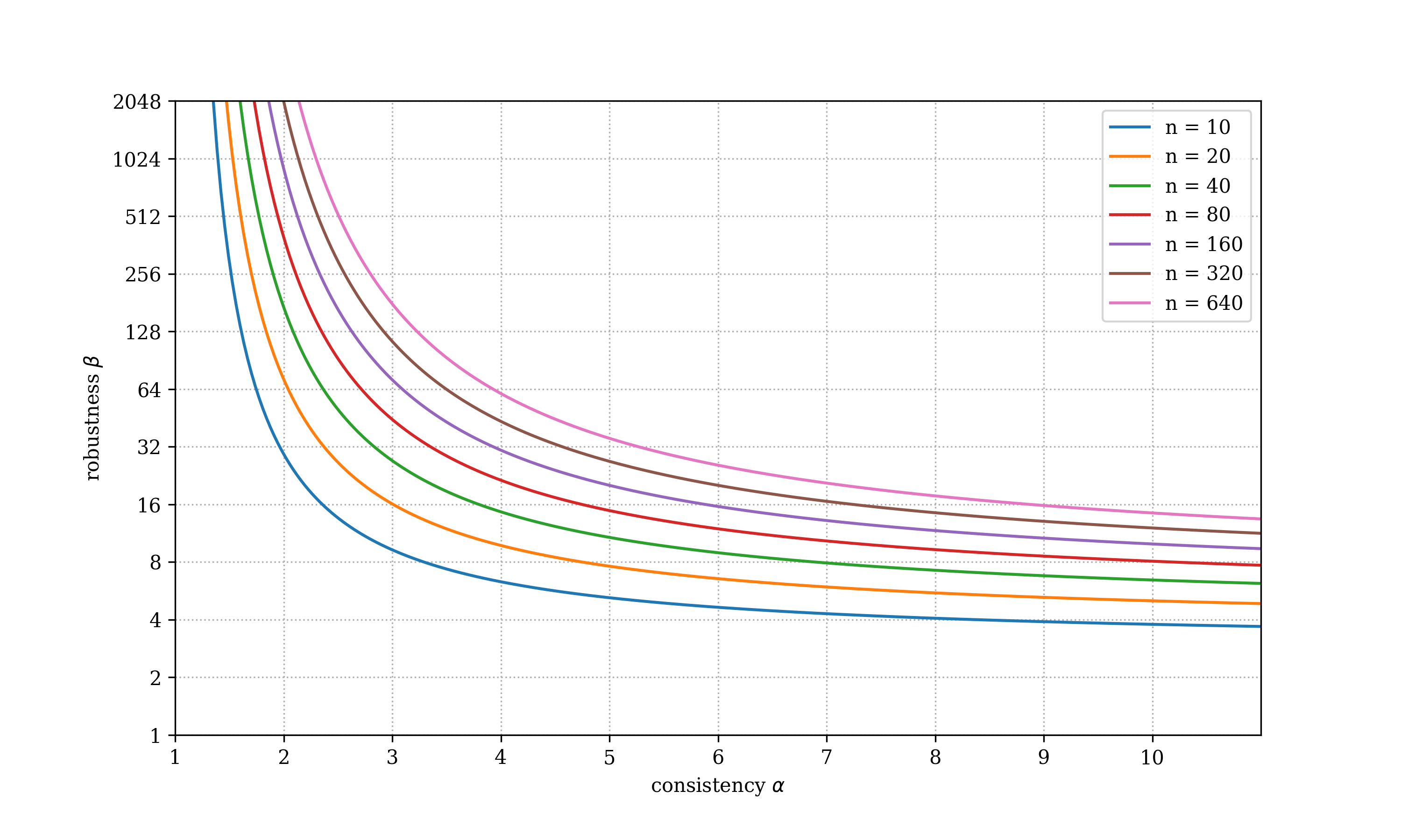
Figure 1: The trade-off between robustness and consistency when $\beta=n^{1/(\alpha-a)}H_{n}$ for different values of $n$

The clock auction, named FollowTheBindingBenchmark, also alternates between uniformly raising the bids of the unpredicted and predicted bidders while maintaining a careful balance between the revenue from the predicted set and the welfare of the unpredicted set. However, to achieve consistency^∞, it requires that in every round, the revenue collected from the predicted set be at least $\frac{1}{\alpha}$ of the rejected welfare of the unpredicted set plus the current revenue, i.e., the lower bound of the welfare of the predicted set. Unless this constraint is satisfied, the clock auction will continue raising the bids for the predicted set. Please see Mechanism 4 for a formal description.

Input: A system $\mathcal{F}$ of feasible sets of bidders, a predicted optimal set $\hat{\texttt{OPT}}$, a consistency parameter $\alpha$, a robustness parameter $\beta$

1

$F\leftarrow F\setminus\{F\cap\hat{\texttt{OPT}}\}$ for all $F\neq\hat{\texttt{OPT}}\in\mathcal{F}$

  // Make $\hat{\texttt{OPT}}$ disjoint from all unpredicted sets

$p_{i}\leftarrow v_{\text{min}}$ for all $i\in N$

  // Raise price of each bidder to the initial small amount

2

3$R^{P}_{0}\leftarrow\text{rev}(\hat{\texttt{OPT}},\mathbf{p})$

4$S\leftarrow\hat{\texttt{OPT}}$

5$t\leftarrow 1$

6while TRUE do

7      Run $\textsc{UniformPrice}(N\setminus\hat{\texttt{OPT}},\mathbf{p})$ until:(i) $\max_{F\in\mathcal{F}}\text{rev}(F\cap N,\mathbf{p})\geq\frac{\beta}{4H_{n}}\cdot R^{P}_{t-1}$; OR (ii) $\max_{F\in\mathcal{F}}v(F\setminus N)\geq\frac{\beta}{4}\cdot R^{P}_{t-1}$ and $\max_{F\in\mathcal{F}}\text{rev}(F\cap N,\mathbf{p})\geq\frac{\beta}{4H_{n}}\cdot R^{P}_{t-1}$

     if $N=\hat{\texttt{OPT}}$ then  return $\hat{\texttt{OPT}}$, $\mathbf{p}$

       // All unpredicted bidders reject case

8     

9      $\tilde{R}^{P}_{t}\leftarrow R^{P}_{t-1}\cdot 2$

10     Run $\textsc{UniformPrice}(\hat{\texttt{OPT}},\mathbf{p})$ until: (i) $\text{rev}(\hat{\texttt{OPT}},\mathbf{p})\geq\tilde{R}^{P}_{t}$ AND (ii) $(\alpha-1)\cdot\text{rev}(\hat{\texttt{OPT}},\mathbf{p})\geq v(S\setminus\hat{\texttt{OPT}})$

     if $\hat{\texttt{OPT}}=\emptyset$ then return WFCA$(N,\mathbf{p})$

       // All predicted bidders reject case

11     

12      $R^{P}_{t}\leftarrow\text{rev}(\hat{\texttt{OPT}},\mathbf{p})$

13     $t\leftarrow t+1$

MECHANISM 4 FollowTheBindingBenchmark

As before, we assume that $\mathcal{F}$ is a set system where the predicted set is completely disjoint from all maximal unpredicted sets. This is without loss by Observation 1. We first prove the robustness guarantee. All the missing proofs can be found in Appendix D.

Robustness Argument

To demonstrate that Mechanism 4 achieves the desired robustness we consider two cases depending on whether or not the auction terminates by serving a subset of the predicted set or a subset of some unpredicted set. Since we assume that $\alpha<\beta$ (and we will eventually show that our mechanism achieves social welfare within a $\alpha$-factor of the welfare in the predicted set), we show that our mechanism obtains welfare within a $\beta$-factor of the best unpredicted set. Building toward this guarantee, we first prove a useful lemma regarding the total welfare lost from an unpredicted set.

Lemma 8.

The total welfare rejected in any unpredicted set $S$ in some iteration $t$ is at most $\frac{\beta}{2}\cdot R^{P}_{t-1}.$

As a corollary of this lemma, we can bound the total welfare lost from any unpredicted set of bidders by observing that the revenue and welfare targets increase by at least a factor $2$ in each round.

Corollary 1.

The total welfare rejected in any unpredicted set $S$ throughout the first $t^{\prime}$ iterations is at most $\beta R^{P}_{t^{\prime}-1}$.

We are now ready to prove the robustness guarantees of the mechanism 4. Similarly as in Section 3 we will analyze cases whether or not the subset of $\hat{\texttt{OPT}}$ is outputted differently. We first consider the case where a subset of $\hat{\texttt{OPT}}$ is outputted. The intuition is that we only serve a subset of predicted bidders if we do not satisfy either condition in Line 4 but we secured good revenue from the predicted set in the previous iteration of the while loop. We formalize this intuition in the following lemma.

Lemma 9.

If Mechanism 4 outputs a subset of the predicted set, then Mechanism 4 is $\beta$-robust.

Proof.

Let $\hat{t}$ denote the value of $t$ when the auction terminates. By assumption that we serve a subset of the predicted set and definition of the mechanism, this was a result of not satisfying either condition in Line 4. Note that we proceeded to round $\hat{t}$ because we satisfied the conditions of Line 4 in round $\hat{t}-1$. As such, the welfare remaining in the the predicted set is at least $R^{P}_{\hat{t}-1}$ (the revenue of the predicted set at the end of the previous round). On the other hand, we know that the total welfare in any unpredicted set (since all unpredicted bidders were rejected) is at most $\beta R^{P}_{\hat{t}-1}$ by Corollary 1. Therefore we obtain welfare within a $\beta$ fraction of the optimal unpredicted set. ∎

We now turn toward the case where a subset of an unpredicted set is output. As in Section 3, we consider the welfare contributions from bidders who exit the auction before the WFCA and those active during the WFCA separately.

Lemma 10.

If Mechanism 4 outputs a subset of some unpredicted set, then Mechanism 4 is $\beta$-robust.

Proof.

Let $\hat{t}$ denote the value of $t$ when the auction terminates. By assumption that we serve a subset of the unpredicted set and definition of the mechanism, the auction terminates in Line 4. We may divide the welfare of the best unpredicted set into two components – the portion of the welfare coming from bidders rejected during before the WFCA is run and the portion of the welfare coming from bidders which are active when the WFCA is run in Line 4. By Corollary 1 we have that the total welfare rejected in any unpredicted set through the first $\hat{t}$ iterations is $\beta R^{P}_{\hat{t}-1}$. On the other hand, we have that the revenue of the best unpredicted set before we run Line 4 is at least $\frac{\beta}{4H_{n}}\cdot R^{P}_{\hat{t}-1}$. In addition, by Lemma 1 we know that the revenue after completing Line 4 must then be at least $\frac{\beta}{4H_{n}}\cdot R^{P}_{\hat{t}-1}$. This gives that the revenue collected by Mechanism 4 is within a $4H_{n}$-factor of the welfare in the best unpredicted set contributed from bidders rejected before Line 4 is run. Moreover, we have by Lemma 1 that the welfare achieved by our auction is within a $2H_{n}$-factor of the welfare in the best unpredicted set contributed from bidders who are active when Line 4 is run. Combining these we have that if a subset of the unpredicted bidders is served then Mechanism 4 obtains welfare within a factor $4H_{n}+2H_{n}\leq\beta$ of the best unpredicted set. ∎

Consistency Argument

We now turn toward the more technically challenging consistency^∞ guarantee. Recall again that a mechanism achieves $\alpha$-consistency^∞ if the it achieves an $\alpha$-approximation to the value of the predicted set, irrespective of the prediction quality. To this end, we first resolve the simpler case where we serve some subset of predicted set. In this case the guarantee is achieved by design, we include a formal proof of this for completeness in Appendix D.

Lemma 11.

If Mechanism 4 outputs a subset of the predicted set, then Mechanism 4 is $\alpha$-consistent^∞.

The more difficult case involves ensuring $\alpha$-consistency^∞given that we output a subset of some unpredicted set. Intuitively we want to argue that by defining a large enough $\beta$, the revenue we obtained from the best unpredicted set is enough to “cover” the maximum potential welfare the predicted set can contain. To this end, we begin with some individual bounds of agent’s value in the predicted set based on when they rejected the price offer.

Lemma 12.

Consider any iteration $t$. At the start of running Line 4, condition (ii) is true. In addition, while (ii) remains true, the current price offered to the bidders is less than $\tilde{R}_{t}^{P}/k$ where $k$ is the number of active bidders in the predicted set.

Proof.

We begin by demonstrating the first part of the lemma statement. First observe that, by design, we satisfied both conditions (i) and (ii) of Line 4 at the end of iteration $t-1$. Furthermore, since we do not raise any prices for predicted bidders in iteration $t$ before reaching Line 4 again, it must be that in iteration $t$ we satisfy condition (ii) at the start of Line 4. For the second part of the lemma statement, suppose that condition (ii) of Line 4 is satisfied and $k$ bidders are active. If we continue to uniformly raise prices for these $k$ bidders, then it must be we do not satisfy condition (i). As such, it must be that these bidders have not yet accepted a price of $\tilde{R}_{t}^{P}/k$. ∎

Claim 1.

Fix a set $S$ and index bidders in $S$ in non-increasing value order. Two conditions hold:

1. Suppose that $(\alpha-1)kv_{k}\leq\sum_{i=k+1}^{|S|}{v_{i}}$. Then, if $(\alpha-1)(k-1)v_{k-1}\geq\sum_{i=k}^{|S|}{v_{i}}$ we have that

   $$v_{k-1}\geq\frac{(\alpha-1)k+1}{(\alpha-1)(k-1)}v_{k}.$$

2. Suppose that $(\alpha-1)kv_{k}\geq\sum_{i=k+1}^{|S|}{v_{i}}$. Then, if $(\alpha-1)(k-1)v_{k-1}\leq\sum_{i=k}^{|S|}{v_{i}}$ we have that

   $$v_{k-1}\leq\frac{(\alpha-1)k+1}{(\alpha-1)(k-1)}v_{k}.$$

Proof.

We show part 1 of the claim as part 2 follows, symmetrically, by flipping the inequalities. By assumption, we have that $\sum_{i=k+1}^{|S|}{v_{i}}\geq(\alpha-1)kv_{k}$ so substituting gives

$$(\alpha-1)(k-1)v_{k-1} \geq\sum_{i=k}^{|S|}{v_{i}}\geq v_{k}+(\alpha-1)kv_{k},$$

or, equivalently,

$$v_{k-1}\geq\frac{(\alpha-1)k+1}{(\alpha-1)(k-1)}v_{k}.\qed$$

Lemma 13.

Consider any point when we are running UniformPrice on the predicted set (i.e., we are running Line 4) where condition (ii) is satisfied and let $k$ denote the number of active bidders in the predicted set. If the smallest valued predicted bidder with value $p_{k}$ rejecting causes condition (ii) to be violated, then if condition (ii) is not satisfied before the $k-1$-th largest bidder exits the auction her value $p_{k-1}$ is upper bounded by

$$p_{k-1}<\frac{(\alpha-1)k+1}{(\alpha-1)(k-1)}\cdot p_{k}.$$ (4)

Proof.

Fix some point in the auction when the revenue of the predicted set satisfied $\alpha$-consistency^∞, i.e., $(\alpha-1)$ times the current predicted revenue is greater than or equal to the rejected welfare in the predicted set, and let $k$ denote the number of remaining active predicted bidders and $\overline{W}$ denote the total rejected welfare at this point. Let $p_{k}$ denote the price offered to these $k$ active bidders just before one of them exits the auction. We then have $(\alpha-1)\cdot kp_{k}\geq\overline{W}$. If the lowest valued bidder among these $k$ exiting the auction causes $\alpha$-consistency^∞ to be violated, i.e., $\alpha\cdot(k-1)p_{k}<p_{k}+\overline{W}$ we may obtain an upper bound on the price $p_{k-1}$ corresponding to the point at which $\alpha$-consistency^∞ would be satisfied again if $k-1$ bidders accept $p_{k-1}$. By applying part 2 of Claim 1, we obtain that

$$p_{k-1}<\frac{(\alpha-1)k+1}{(\alpha-1)(k-1)}\cdot p_{k}.\qed$$

Observation 2.

For any $k>2$ and $\alpha>1$ we have that

$$\frac{1}{k-1}\leq\frac{1}{k}\cdot\frac{(\alpha-1)k+1}{(\alpha-1)(k-1)}=\frac{1}{k-1}+\frac{1}{k(\alpha-1)(k-1)}.$$

With Lemma 13 and Observation 2 in hand we can now move to show that the auction achieves $\alpha$-consistency^∞ when a subset of the unpredicted set is output provided we have $\beta$ large enough. A crucial function in both the upper and lower bounds we demonstrate is $\Gamma(x)$ where $\Gamma(x)=\int_{0}^{\infty}{t^{x-1}e^{-t}dt}$ is the extension of the factorial function to the complex numbers, i.e., $\Gamma(k)=(k-1)!$ for $k\in\mathbb{N}$.

Lemma 14.

If Mechanism 4 with parameters $\alpha\in[1+\epsilon,H_{n}]$ and

$$\beta\geq\frac{8H_{n}\Gamma\left(n+\frac{\alpha}{\alpha-1}\right)}{\Gamma\left(1+\frac{\alpha}{\alpha-1}\right)n!}-\frac{4H_{n}(\alpha-1)}{\alpha}=\Theta\left(n^{\frac{1}{\alpha-1}}\log n\right)$$

outputs a subset of some unpredicted set, then it is $\alpha$-consistent^∞.

Proof.

Consider the round $\hat{t}$ in which the auction terminates and assume that the auction proceeds to Line 4, i.e., a subset of the unpredicted bidders is served. By Lemma 12, note that the revenue $R^{P}_{\hat{t}-1}$ reached by the predicted set in iteration $\hat{t}-1$ was such that $(\alpha-1)\cdot R^{P}_{\hat{t}-1}$ was more than the total rejected welfare in the predicted set throughout the first $\hat{t}-1$ iterations of the while loop, i.e., the iteration $\hat{t}-1$ concluded with the predicted set satisfying $\alpha$-consistency^∞. On the other hand, since we proceeded past Line 4 we have that the revenue in the unpredicted set reached at least $\frac{\beta}{4H_{n}}\cdot R^{P}_{\hat{t}-1}$. We just then want to bound the total welfare lost from the predicted set in the final iteration $\hat{t}$. By Lemma 12 we have that the first rejected bidder has value at most $2R^{P}_{\hat{t}-1}/k$ where $k$ is the number of active predicted bidders at the start of iteration $\hat{t}$. Applying Lemma 13 and Observation 2 to upper bound the value $v_{k-1}$ of the next rejecting bidder, we obtain that

$$v_{k-1}\leq\frac{2R^{P}_{\hat{t}-1}}{k}\cdot\frac{(\alpha-1)k+1}{(\alpha-1)(k-1)}.$$

Iteratively applying Lemma 13 and Observation 2 to find an upper bound to each rejected bidder’s value, we have that the total welfare rejected in this round is at most

$$\frac{2R^{P}_{\hat{t}-1}}{k}+\sum_{i=2}^{k}{\frac{2R^{P}_{\hat{t}-1}}{k}\cdot\prod_{j=i}^{k}\frac{(\alpha-1)j+1}{(\alpha-1)(j-1)}} \leq\frac{2R^{P}_{\hat{t}-1}}{n}+\sum_{i=2}^{n}{\frac{2R^{P}_{\hat{t}-1}}{n}\cdot\prod_{j=i}^{n}\frac{(\alpha-1)j+1}{(\alpha-1)(j-1)}}$$

$$=\frac{2R^{P}_{\hat{t}-1}}{n}+\frac{2R^{P}_{\hat{t}-1}}{n}\cdot\sum_{i=2}^{n}{\prod_{j=i}^{n}\frac{j+1/(\alpha-1)}{j-1}}$$

$$=\frac{2R^{P}_{\hat{t}-1}}{n}+\frac{2R^{P}_{\hat{t}-1}}{n}\cdot\sum_{i=2}^{n}{\frac{\Gamma(i-1)\Gamma\left(n+1+\frac{1}{\alpha-1}\right)}{\Gamma\left(\frac{1}{\alpha-1}+i\right)\Gamma(n)}}$$

$$=\frac{2R^{P}_{\hat{t}-1}}{n}+\frac{2R^{P}_{\hat{t}-1}}{n}\cdot\left(-\alpha n+\frac{\alpha\Gamma\left(\frac{n\alpha+\alpha-n}{\alpha-1}\right)}{\Gamma\left(\frac{2\alpha-1}{\alpha-1}\right)\Gamma(n)}+n-1\right)$$

$$=\frac{2R^{P}_{\hat{t}-1}}{n}\cdot\left(-\alpha n+\frac{\alpha\Gamma\left(\frac{n\alpha+\alpha-n}{\alpha-1}\right)}{\Gamma\left(\frac{2\alpha-1}{\alpha-1}\right)(n-1)!}+n\right),$$

where the inequality comes from the fact that for any $\alpha>1$ the partial product from $j=k+1$ to $n$ times $2R^{P}_{\hat{t}-1}/n$ yields a value at least $2R^{P}_{\hat{t}-1}/k$, the second equality comes from the fact that $z\cdot\Gamma(z)=\Gamma(z+1)$ for all $z\in\mathbb{R}$ and, hence, $\Gamma(x+y)/\Gamma(x)=x\cdot(x+1)\cdot\dots\cdot(x+y-1)$ for all $y\in\mathbb{N}$ and all $x\in\mathbb{R}$, and the third equality is due to Lemma 19 which we defer to Appendix E.

Combining the welfare rejected from the first $\hat{t}-1$ rounds and the welfare from the last round we obtain that the total welfare rejected from the predicted set is at most

$$(\alpha-1)\cdot R^{P}_{\hat{t}-1}+\frac{2R^{P}_{\hat{t}-1}}{n}\cdot\left(-\alpha n+\frac{\alpha\Gamma\left(\frac{n\alpha+\alpha-n}{\alpha-1}\right)}{\Gamma\left(\frac{2\alpha-1}{\alpha-1}\right)(n-1)!}+n\right).$$

But then, since our auction reached revenue at least $\frac{\beta}{4H_{n}}\cdot R^{P}_{\hat{t}-1}$ before running the WFCA and the WFCA is revenue monotone by Lemma 1 it suffices that

$$\alpha\frac{\beta}{4H_{n}}\geq(\alpha-1)+\frac{2}{n}\cdot\left(-\alpha n+\frac{\alpha\Gamma\left(\frac{n\alpha+\alpha-n}{\alpha-1}\right)}{\Gamma\left(\frac{2\alpha-1}{\alpha-1}\right)(n-1)!}+n\right)$$

or, equivalently,

$$\beta\geq\frac{4H_{n}}{\alpha}\cdot\left((\alpha-1)+\frac{2}{n}\cdot\left(-\alpha n+\frac{\alpha\Gamma\left(\frac{n\alpha+\alpha-n}{\alpha-1}\right)}{\Gamma\left(\frac{2\alpha-1}{\alpha-1}\right)(n-1)!}+n\right)\right).$$

Therefore, for the proof to go through it suffices for $\beta$ to satisfy

$$\beta~{}\geq~{}\frac{4H_{n}}{\alpha}(\alpha-1-2\alpha+2)+\frac{8H_{n}\Gamma\left(n+\frac{\alpha}{\alpha-1}\right)}{\Gamma\left(1+\frac{\alpha}{\alpha-1}\right)n!}~{}=~{}\frac{8H_{n}\Gamma\left(n+\frac{\alpha}{\alpha-1}\right)}{\Gamma\left(1+\frac{\alpha}{\alpha-1}\right)n!}-\frac{4H_{n}(\alpha-1)}{\alpha}.$$

As we care about the asymptotic behavior of this bound and $n+\frac{\alpha}{\alpha+1}$ is a positive real number, we can apply Stirling’s approximation, i.e.,

$$\Gamma(z)=\sqrt{\frac{2\pi}{z}}\left(\frac{z}{e}\right)^{z}\left(1+O\left(\frac{1}{z}\right)\right),$$

to obtain that the proof goes through with

$$\beta =\frac{8H_{n}}{\Gamma\left(1+\frac{\alpha}{\alpha-1}\right)}\cdot\frac{\sqrt{\frac{2\pi}{n+1+1/(\alpha-1)}}\left(\frac{n+1+1/(\alpha-1)}{e}\right)^{n+1+1/(\alpha-1)}\left(1+O\left(\frac{1}{n+1+1/(\alpha-1)}\right)\right)}{\sqrt{\frac{2\pi}{n+1}}\left(\frac{n+1}{e}\right)^{n+1}\left(1+O\left(\frac{1}{n+1}\right)\right)}$$

$$=\frac{8H_{n}}{\Gamma\left(1+\frac{\alpha}{\alpha-1}\right)}\cdot O(1)\cdot\left(\frac{n+1+1/(\alpha-1)}{e}\right)^{n+1+1/(\alpha-1)}\cdot\left(\frac{e}{n+1}\right)^{n+1}$$

$$=\frac{8H_{n}}{\Gamma\left(1+\frac{\alpha}{\alpha-1}\right)}\cdot O(1)\cdot\frac{(n+1+1/(\alpha-1))^{n+1+1/(\alpha-1)}}{(n+1)^{n+1}}\cdot\frac{1}{e^{1/(\alpha-1)}}$$

$$=\Theta\left(n^{\frac{1}{\alpha-1}}\log n\right)$$

where the last line is since $\Gamma(c)$ is a constant for any constant real number $c$ and $H_{n}\geq\alpha>1+\epsilon$ for constant $\epsilon>0$ so $1/(\alpha-1)=O(1)$ and $\Gamma(1+\alpha/(\alpha-1))=O(1)$. ∎

4.1 Lower Bound

We now show that the guarantee that Mechanism 4 obtained is asymptotically tight.

Theorem 5.

The robustness of any deterministic clock auction that is augmented with a prediction $\hat{\texttt{OPT}}$ and satisfies $\alpha$-consistency^∞for $\alpha\in[1+\epsilon,H_{n}]$ is $\Omega(n^{1/(\alpha-1)}\log{n})$

Proof.

Consider a feasibility constraint $\mathcal{F}$ defined by two disjoint maximal feasible sets $F_{1}$ and $F_{2}$, i.e., $N=F_{1}\cup F_{2}$, and a set $F\subseteq N$ is feasible if and only if $F\subseteq F_{1}$ or $F\subseteq F_{2}$. Let the sizes of these sets be $|F_{1}|=k_{1}$ and $|F_{2}|=k_{2}$, and let $F_{2}$ be the set predicted to be optimal, i.e., $\hat{\texttt{OPT}}=F_{2}$.

Using this feasibility constraint, we now define a family of instances $\mathcal{I}$ by defining the set of values that can be assigned to the bidders in $F_{1}$ and the bidders in $F_{2}$; the class of instances in $\mathcal{I}$ corresponds to all possible assignments of these values to the bidders in the corresponding sets. Let

$$V_{1}=\left\{1,\frac{1}{2},\frac{1}{3},\dots,\frac{1}{k_{1}}\right\}$$

be a set of $k_{1}$ values that can be matched to the $k_{1}$ bidders in $F_{1}$ and let

$$V_{2}=\{v_{1},v_{2},\dots,v_{k_{2}}\}$$

be a set of $k_{2}$ values that can be matched to the $k_{2}$ bidders in $F_{2}$, such that the highest value among them is $v_{1}=1$ and the rest of the sequence is decreasing such that for every $i\in\{2,3,\dots,k_{2}\}$:

$$v_{i}=\frac{(\alpha-1)(i-1)+\delta}{(\alpha-1)i+1}\cdot v_{i-1},$$

where $\delta>0$ is some arbitrarily small constant. Note that as $\delta\to 0$ and $\alpha\to\infty$, this sequence of values converges to the harmonic sequence $\left\{1,\frac{1}{2},\frac{1}{3},\dots,\frac{1}{k_{2}}\right\}$. However, for smaller values of $\alpha$ the values in $V_{2}$ drop much faster than that. Specifically, the lowest value in $V_{2}$ is

$$v_{k_{2}}~{}=~{}\prod_{i=2}^{k_{2}}\frac{(\alpha-1)(i-1)+\delta}{(\alpha-1)i+1}~{}=~{}\frac{\Gamma\left(1+\frac{\alpha}{\alpha-1}\right)(k_{2}-1)!}{\Gamma\left(k_{2}+\frac{\alpha}{\alpha-1}\right)}+\delta^{\prime},$$ (5)

where $\delta^{\prime}\to 0$ as $\delta\to 0$. One of the crucial properties of the values in $V_{2}$ is that based on the rate of growth and part 1 of Claim 1, for every $i\in\{1,2,\dots,k_{2}-1\}$ it satisfies:

$$(\alpha-1)\cdot i\cdot v_{i}<\sum_{j=i+1}^{k_{2}}v_{j}.$$ (6)

To prove this theorem, we consider any learning-augmented clock auction $\mathcal{M}$ and simulate it on an instance from $\mathcal{I}$, chosen adversarially to maximize the number of bidders that drop out. Note that, since $\mathcal{M}$ is deterministic, the adversary can essentially determine who to assign each value to after observing the price trajectory that $\mathcal{M}$ will follow. Specifically, whenever $\mathcal{M}$ raises the price of an active bidder $i\in F_{1}$ to an amount that exceeds some value $v\in V_{1}$ that remains active (i.e., that was not already assigned to a bidder that has dropped out), then the adversary can assign the value $v$ to $i$ and, as a result, $i$ drops out. This implies that, if at any point during the execution of $\mathcal{M}$ the maximum price offered to an active bidder in $F_{1}$ is $p_{1}$, then the value of every active bidder in $F_{1}$ is at least $p_{1}$ (otherwise the adversary could have assigned that value to the bidder facing price $p_{1}$, causing him to drop out). Using the same argument for $F_{2}$, we can conclude that if at any point during the execution of $\mathcal{M}$ the maximum price offered to an active bidder in $F_{2}$ is $p_{2}$, then the values of all active bidders in $F_{2}$ are at least $p_{2}$.

We now partition the set of all clock auctions into three cases, based on their outcome facing the adversarially chosen instance from $\mathcal{I}.$

Case 1 (the auction $\mathcal{M}$ accepts a subset of $F_{1}$): For this case, we show that there exists an instance (not in $\mathcal{I}$) for which the auction fails to achieve $\alpha$-consistency^∞. To verify this, let $x$ be the number of bidders in $F_{1}$ that did not drop out and note that, given the harmonic structure of the values in $V_{1}$, the smallest value among them will be at most $1/x$. As we showed above, this means that the maximum price offered to any one of the winning bidders in $F_{1}$ was $p_{1}\leq 1/x$. Now, consider an alternative instance that is identical in terms of the values of all the bidders that dropped out, but has value $1/x$ for all of the bidders that won. Note that the outcome of the auction would be the same for this alternative instance, since the only difference is regarding values of bidders that are higher than the price offered to them, so the welfare achieved by $\mathcal{M}$ in this alternative instance would be $x\cdot\frac{1}{x}=1$. However, the social welfare of $\hat{\texttt{OPT}}=F_{2}$ is more than $\alpha$, which is implied by Inequality (6) for $i=1$, which violates the $\alpha$-consistency^∞ constraint.

Case 2 (the auction $\mathcal{M}$ accepts a strict subset of $\hat{\texttt{OPT}}$): For this case, we once again show that there exists an instance (not in $\mathcal{I}$) for which the auction fails to achieve $\alpha$-consistency^∞. To verify this, let $x\leq k_{2}-1$ be the number of bidder in $\hat{\texttt{OPT}}$ that did not drop out and note that, by the definition of the values in $V_{2}$, the smallest value among them is $v_{x}$. As we showed above, this means that the maximum price offered to any one of the winning bidders in $\hat{\texttt{OPT}}$ was $p_{2}\leq v_{x}$. We, once again, consider the alternative instance that is identical in terms of the values of all the bidders that dropped out, but has value $v_{x}$ for all the bidders in $\hat{\texttt{OPT}}$ that won. The outcome of the auction would not be affected by this change, so the resulting welfare would be $x\cdot v_{x}$ but, using Inequality (6) for $i=x$, this violates the $\alpha$-consistency^∞ constraint.

Case 3 (the auction $\mathcal{M}$ accepts every bidder in $\hat{\texttt{OPT}}$): For this case, note that no price offered to a bidder in $\hat{\texttt{OPT}}$ exceeded $v_{k_{2}}$, otherwise the adversarial assignment of values would ensure that the corresponding bidder would have dropped out and $\mathcal{M}$ would not accept all of them. Now consider consider an alternative instance that is identical with respect to the values of the bidders in $F_{1}$, but the values of everyone in $F_{2}$ are equal to $v_{k_{2}}$. Note that the outcome of the auction would be the same in this alternative instance, since the only difference is regarding values of bidders that are higher than the price offered to them. Therefore, using Equation (5), we can conclude that the welfare achieved by the auction in this instance would be

$$k_{2}\cdot v_{k_{2}}=k_{2}\cdot\frac{\Gamma\left(1+\frac{\alpha}{\alpha-1}\right)(k_{2}-1)!}{\Gamma\left(k_{2}+\frac{\alpha}{\alpha-1}\right)}+\delta^{\prime}=\frac{\Gamma\left(1+\frac{\alpha}{\alpha-1}\right)k_{2}!}{\Gamma\left(k_{2}+\frac{\alpha}{\alpha-1}\right)}+\delta^{\prime},$$

whereas the welfare of $F_{1}$ is equal to $H_{k_{1}}=1+\frac{1}{2}+\dots+\frac{1}{k_{1}}$, leading to a robustness of

$$\beta=\Omega\left(\frac{H_{k_{1}}\Gamma\left(k_{2}+\frac{\alpha}{\alpha-1}\right)}{\Gamma\left(1+\frac{\alpha}{\alpha-1}\right)k_{2}!}\right)=\Omega\left(k_{2}^{1/(\alpha-1)}\log{k_{1}}\right),$$

where the last equation is inferred by following the same steps as we did at the end of the proof of Lemma 14. If we let $k_{1}=n^{c}$ and $k_{2}=n-n^{c}$ for any constant $c>0$, this yields the claimed robustness lower bound. ∎

Appendix A Missing Proofs from Section 3

A.1 Proof of Lemma 2

Proof.

Fix some set $S$ and consider the process of raising the price offered to bidders in this set as in line 2. If at least $k$ bidders in $S$ accept a price of $R_{t}/k$ for any $k$ then we terminate this process (since the total revenue in $S$ would reach the revenue target of $R_{t}$). This would happen if the $k$-th highest value bidder in $S$ had value more than $R_{t}/k$. As such, rejecting the $k^{\prime}$-th highest value bidder in iteration $t$ of the while loop implies that this bidder has value at most $R_{t}/k^{\prime}$. On the other hand, since there are at most $n$ bidders contained in set $S$ the total value of the bidders rejected in iteration $i$ of the while loop is at most

$$\sum_{k^{\prime}=1}^{n}{\frac{R_{t}}{k^{\prime}}}=R_{t}\cdot H_{n}.\qed$$

A.2 Proof of Lemma 6

Proof.

Following the same argument of Lemma 2 we first observe that the total welfare rejected from the predicted set in line 5 in any iteration $t^{\prime}$ of the while loop of FollowTheUnpredictedLeader is at most $R_{t^{\prime}}\cdot H_{n}$. Taking a sum over all rounds from $1$ to $t$ we then obtain that the total welfare rejected is at most

$$\sum_{t^{\prime}=1}^{t}{R_{i^{\prime}}\cdot H_{n}}=H_{n}\sum_{t^{\prime}=1}^{t}{10^{t^{\prime}}}=H_{n}\cdot\frac{10^{t+1}-1}{9}\leq R_{t}\cdot\frac{10H_{n}}{9}\qed$$

Appendix B Missing Proof from Section 3.1

Proof of Theorem 2.

Consider any deterministic clock auction $\mathcal{M}$ that is augmented with a prediction $\hat{\texttt{OPT}}$ and achieves $(1+\epsilon)$-consistency and robustness better than $\Omega(\frac{1}{\epsilon}\log{n})$. Also, consider a family of instances involving an arbitrarily large number of bidders $n$ and a feasibility constraint $\mathcal{F}$ defined by two disjoint maximal feasible sets $F_{1}$ and $F_{2}$, i.e., $N=F_{1}\cup F_{2}$, and a set $F\subseteq N$ is feasible if and only if $F\subseteq F_{1}$ or $F\subseteq F_{2}$. $F_{1}$ contains only a single bidder and $|F_{2}|=n-1$. Also, let $F_{2}$ be the set predicted to be optimal, i.e., $\hat{\texttt{OPT}}=F_{2}$.

Using this feasibility constraint, we now define a family of instances $\mathcal{I}$ where the value of the single bidder in $F_{1}$ is $0.99$ and the values of the bidders in $F_{2}$ correspond to the following set of values:

$$V_{2}=\left\{0.99,\frac{\epsilon}{2(H_{n-1}-1)},\frac{\epsilon}{3(H_{n-1}-1)},\dots,\frac{\epsilon}{(n-1)(H_{n-1}-1)}\right\}.$$

We now consider what $\mathcal{M}$ does facing an instance in $\mathcal{I}$ that is chosen by adversarially matching the values in $V_{2}$ to bidders in $F_{2}$, depending on the deterministic price trajectory that $\mathcal{M}$ will follow. Specifically, at each time $t$ during the execution of $\mathcal{M}$, let $V_{2}(t)\subseteq V_{2}$ be the set of values from $V_{2}$ assigned to bidders that have not dropped out yet. Then, the adversarial assignment of values to bidders in $F_{2}$ ensure that if at any time $t$ the price offered to an active bidder $i\in F_{2}$ exceeds a value $v\in V_{2}(t)$, we can assume that the adversary assigns $v$ to $i$, so $i$ would drop out. As a result, if number of active bidders at any time $t$ is $x\geq 2$, then the highest value offered to any one of them is at most $\frac{\epsilon}{x(H_{n-1}-1)}$, so the revenue never exceeds $x\cdot\frac{\epsilon}{x(H_{n-1}-1)}=\frac{\epsilon}{H_{n-1}-1}$.

Using this fact, with the assumption that the auction achieves better than $\Omega(\frac{1}{\epsilon}\log n)$, we can infer that the auction cannot terminate with at least two active bidder in $F_{2}$. Specifically, if $\mathcal{M}$ terminated with $x\geq 2$ active bidders in $F_{2}$ and, as we argued above, their final price was at most $\frac{\epsilon}{x(H_{n-1}-1)}$, then $\mathcal{M}$ would fail to satisfy the claimed robustness guarantee on an alternative instance (not in $\mathcal{I}$). This alternative instance is identical in terms of the values of all the bidders that dropped out and the only difference is in the value of the $x$ winning bidders, whose values are changed to $\frac{\epsilon}{x(H_{n-1}-1)}$. Note that the outcome of $\mathcal{M}$ facing this alternative instance would be the same, since the prices offered to the winning bidders would still be below their values. However, in this alternative instance the welfare of $\mathcal{M}$ would be $\frac{\epsilon}{H_{n-1}-1}$ while the optimal social welfare is $0.99$, leading to a robustness of $\Omega(\frac{1}{\epsilon}\log{n})$.

If, on the other hand, the auction accepted at most 1 bidder from $F_{2}$, then the resulting welfare would be $0.99$. Consider the total value rejected so far, we would have: $\sum^{n-1}_{i=2}\frac{\epsilon}{i\cdot(H_{n-1}-1)}=\epsilon,$ since $\sum^{n-1}_{i=2}=H_{n-1}-1$. Therefore the consistency would be

$$\frac{0.99+\epsilon}{0.99}>1+\epsilon,$$

violating the consistency guarantee. ∎

Appendix C Missing Proof from Section 3.2

For completeness we include the full description of ErrorTolerant below:

Input: A system $\mathcal{F}$ of feasible sets of bidders, a predicted optimal set $\hat{\texttt{OPT}}$, a parameter $\gamma$

1

$F\leftarrow F\setminus\{F\cap\hat{\texttt{OPT}}\}$ for all $F\neq\hat{\texttt{OPT}}\in\mathcal{F}$

  // Make $\hat{\texttt{OPT}}$ disjoint from all unpredicted sets

2

$p_{i}\leftarrow v_{\text{min}}$ for all $i\in N$

  // Raise price of each bidder to the initial small amount

3 $R_{0}\leftarrow\text{rev}(\hat{\texttt{OPT}},\mathbf{p})$

$t\leftarrow 1$

  // Initialize the counter

4

5while TRUE do

6      $R_{t}\leftarrow 10^{t}R_{t-1}$

     Run $\textsc{UniformPrice}(N\setminus\hat{\texttt{OPT}},\mathbf{p})$ until $\max_{F}v(F\setminus N)\in[R_{t}\gamma H_{n},2R_{t}\gamma H_{n})$

       // Reject ‘‘safe’’ amount of welfare to determine minimum total value in optimal set

7     

8     if $N=\hat{\texttt{OPT}}$ then  return $\hat{\texttt{OPT}}$, $\mathbf{p}$

9     

     Run $\textsc{UniformPrice}(N\setminus\hat{\texttt{OPT}},\mathbf{p})$ until $\max_{F}\text{rev}(F\cap N,\mathbf{p})\geq R_{t}$

       // Ensure unpredicted sets ‘‘cover’’ their own lost welfare

10     

11     if $N=\hat{\texttt{OPT}}$ then  return $\hat{\texttt{OPT}}$, $\mathbf{p}$

      Run $\textsc{UniformPrice}(\hat{\texttt{OPT}},\mathbf{p})$ until $\text{rev}(\hat{\texttt{OPT}},\mathbf{p})\geq R_{t}/\overline{\eta}$

       // Ensure predicted set ‘‘covers’’ welfare lost from unpredicted sets

12     

13     if $\hat{\texttt{OPT}}=\emptyset$ then

14           return WFCA$(N,\mathbf{p})$

15          

16          $t\leftarrow t+1$

MECHANISM 5 ErrorTolerant

Lemma 15.

Suppose that the predicted set has total welfare at least $1/\overline{\eta}$ times the optimal social welfare (i.e., the prediction is within the error tolerance). Then for a fixed parameter $\gamma>10/9$ ErrorTolerant terminates in either Line 5 or Line 5 and obtains at least a $\left(1-\frac{10}{9\gamma}\right)$-fraction of the social welfare of the predicted set.

Proof.

Fix an instance $I$ where the optimal set has social welfare $W^{*}$ and where the predicted set has welfare at least $W^{*}/\overline{\eta}$. Consider the minimum value $k$ such that $10^{k}\cdot\gamma H_{n}$ exceeds $W^{*}$. Let $i^{\prime}$ denote the value of $i$ at the beginning of the final iteration of the while loop of ErrorTolerant when run on instance $I$. Since we only continue to line 5 after the preceding if statement when there are still active unpredicted bidders it must be that $i^{\prime}\leq k$ (as, otherwise, some unpredicted set would have total welfare greater than $W^{*}$) and if $i^{\prime}=k$ then we terminate before line 5 (i.e., before we cause any additional predicted bidders to exit the auction in the iteration $k$).

Now consider the total amount of welfare lost from the predicted set from rounds $1$ to $i^{\prime}-1$. By Lemma 6 we have that this total welfare is at most $\frac{R_{i^{\prime}-1}}{\overline{\eta}}\cdot 10H_{n}/9=\frac{10^{i^{\prime}-1}}{\overline{\eta}}\cdot\frac{10H_{n}}{9}\leq\frac{10^{i^{*}-1}}{\overline{\eta}}\cdot\frac{10H_{n}}{9}$. On the other hand, by our definition of $k$, we know that the total social welfare in the predicted set is at least $\frac{10^{k-1}}{\overline{\eta}}\cdot\gamma H_{n}$. But then, at the end of the $i^{\prime}-1$ iteration there must be active predicted bidders and moreover, we retain at least a

$$\frac{\frac{10^{k-1}}{\overline{\eta}}\cdot\gamma H_{n}-\frac{10^{k-1}}{\overline{\eta}}\cdot\frac{10}{9}H_{n}}{\frac{10^{k-1}}{\overline{\eta}}\cdot\gamma H_{n}}=\frac{\gamma-\frac{10}{9}}{\gamma}$$

fraction of the social welfare of the predicted set. ∎

Lemma 16.

Consider some fixed constant parameter $\gamma>10/9$ ErrorTolerant outputs a subset of the predicted set. Then ErrorTolerant obtains social welfare within a $\frac{9}{\overline{\eta}\cdot 100(2\gamma+1)H_{n}}$-factor of the optimal social welfare.

Proof.

Consider the iteration $\hat{t}$ in which the while loop of ErrorTolerant terminates. By definition, the mechanism terminates in either line 5 or line 5. By Line 5 and Lemma 2 we have that the total welfare rejected from any unpredicted set in any round $\hat{t}$ is at most $2W_{\hat{t}}+R_{\hat{t}}H_{n}=R_{\hat{t}}\cdot(2\gamma+1)H_{n}$. But then, summing over all rounds we have that the total welfare contained in any unpredicted set is at most

$$\sum_{\hat{t}=1}^{\hat{t}}{R_{\hat{t}}\cdot(2\gamma+1)H_{n}}=(2\gamma+1)H_{n}\cdot\sum_{\hat{t}=1}^{\hat{t}}{10^{\hat{t}}}=(2\gamma+1)H_{n}\cdot\frac{10^{\hat{t}+1}-1}{9}\leq R_{\hat{t}}\cdot\frac{(2\gamma+1)10H_{n}}{9}.$$

On the other hand, since we continued to iteration $\hat{t}$ we have that the revenue of the bidders in the predicted set reached $\frac{R_{\hat{t}-1}}{\overline{\eta}}=\frac{R_{\hat{t}}}{10\overline{\eta}}$. Moreover, this means that the welfare of the active predicted bidders is at least $\frac{R_{\hat{t}}}{10\overline{\eta}}$ and we serve all these bidders. Hence, ErrorTolerant obtains at least a $\frac{R_{\hat{t}}/(10\overline{\eta})}{R_{\hat{t}}\cdot\frac{(2\gamma+1)10H_{n}}{9}}=\frac{9}{\overline{\eta}\cdot 100(2\gamma+1)H_{n}}$-fraction of the optimal social welfare. ∎

Lemma 17.

Consider some parameter $\gamma>10/9$ ErrorTolerant reaches line 5. Then the revenue of active bidders in the highest revenue set before running the Water-filling Clock Auction is at least a $\frac{9}{10(2\gamma+1)H_{n}}$-approximation of the maximum social welfare obtainable by rejected unpredicted bidders.

Proof.

As before we consider the iteration $\hat{t}$ in which the while loop of ErrorTolerant terminates. By assumption, our while loop terminates in line 5. Following the same reasoning as Lemma 16, the total welfare rejected from any unpredicted set over all rounds from $1$ to $\hat{t}$ is at most

$$\sum_{i^{\prime}=1}^{\hat{t}}{R_{i^{\prime}}\cdot(2\gamma+1)H_{n}}\leq R_{\hat{t}}\cdot\frac{(2\gamma+1)10H_{n}}{9}.$$

On the other hand, because we arrive at line 5 we know that there exists some set unpredicted set which obtains revenue $R_{\hat{t}}$ in round $\hat{t}$. Thus, the revenue among active bidders in the highest revenue set when we reach line 5 is a $\frac{9}{10(2\gamma+1)H_{n}}$-fraction of the maximum social welfare obtained from any feasible set of rejected unpredicted bidders. ∎

Lemma 18.

Consider some parameter $\gamma>10/9$ ErrorTolerant outputs a subset of unpredicted bidders. Then ErrorTolerant obtains social welfare within a $\frac{9}{10(2\gamma+1)H_{n}}+\frac{1}{4\log{n}}$-approximation to the optimal social welfare.

Proof.

In the case that ErrorTolerant outputs a subset of unpredicted bidders it must arrive at line 5. As such, we can decompose the social welfare from the optimal (unpredicted) set into two components, the portion of the welfare coming from bidders rejected before ErrorTolerant runs the Water-filling Clock Auction and the portion of the welfare coming from bidders who participate in the WFCA. From Lemma 17 we know that the revenue reached by ErrorTolerant before running the WFCA is within a $\frac{9}{10(2\gamma+1)H_{n}}$-factor of the welfare rejected from the optimal set before running the WFCA. Moreover, from Lemma 1 we have that the revenue reached by ErrorTolerant after running the WFCA is weakly higher than the revenue reached before running the WFCA. As such, since the welfare obtained by serving a set of bidders is always weakly higher than the revenue collected from these bidders we have that the social welfare obtained by ErrorTolerant is within a $\frac{9}{10(2\gamma+1)H_{n}}$-factor of the welfare rejected from the optimal set before running the WFCA. Finally, we have from Lemma 1 that the social welfare achieved by running the WFCA only on bidders who are active when line 5 is reached is within a $1/(4\log{n})$-factor of the optimal social welfare achievable from these bidders. Combining these two guarantees, we have that the social welfare obtained by ErrorTolerant is within a $\frac{9}{10(2\gamma+1)H_{n}}+\frac{1}{4\log{n}}$-factor of the optimal social welfare. ∎

Proof of Theorem 3.

First observe that $\epsilon>0$ ensures that $\gamma>10/9$. In the case that the predicted set, indeed, has social welfare at least $1/\overline{\eta}$ times the optimal social welfare then Lemma 15 gives that some subset of the predicted set is served. Moreover, we obtain that the total social welfare of served bidders is within a factor

$$\left(1-\frac{10}{9\gamma}\right)=\left(1-\frac{10}{9\frac{10(1+\epsilon)}{9\epsilon}}\right)=\frac{1}{1+\epsilon}$$

of the total social welfare in the predicted set, thereby guaranteeing $(1+\epsilon)\eta$ approximation with error tolerance $\overline{\eta}$. On the other hand, if the predicted set has welfare less than $1/\overline{\eta}$ times the optimal (i.e., $\eta\leq\overline{\eta}$) then we can consider two cases depending on whether or not a subset of the predicted set is ultimately served. If some subset of the predicted set is served, Lemma 16 guarantees that the total social welfare obtained by ErrorTolerant is within a factor $\frac{9}{\overline{\eta}\cdot 100(2\gamma+1)H_{n}}$ of the optimal social welfare. Since $H_{n}=\Theta(\log{n})$ and $\gamma$ is a constant for any choice of constant $\epsilon$ we obtain $\Theta(\log{n})$-robustness in this case when $\overline{\eta}=\Theta(1)$. Finally, if some subset of an unpredicted set is served, Lemma 18 guarantees that ErrorTolerant obtains welfare within a factor $\frac{9}{10(2\gamma+1)H_{n}}+\frac{1}{4\log{n}}$ of the optimal social welfare. Again, since $H_{n}=\Theta(\log{n})$ and $\gamma$ is constant for any constant $\epsilon$ we obtain $\Theta(\log{n})$-robustness in this case, completing the proof. ∎

Appendix D Missing Proofs from Section 4

D.1 Proof of Lemma 8

Proof.

Fix a round $t$ in our auction and consider the total welfare lost by some unpredicted set $S$ in Line 4 during $t$. First observe that if we move to Line 4 as a result of satisfying the second condition of the price increase for the unpredicted sets then it must be that every unpredicted set has rejected welfare less than $\frac{\beta}{4}\cdot R^{P}_{t-1}$ (since we would have otherwise have stopped raising prices sooner, having met the lower revenue target of $\frac{\beta}{4H_{n}}\cdot R^{P}_{t-1}$ before reaching $\frac{\beta}{2}\cdot R^{P}_{t-1}$). On the other hand, suppose we move to Line 4 as a result of satisfying the first condition. Once some unpredicted set has rejected welfare $\frac{\beta}{4}\cdot R^{P}_{t-1}$, this condition will be satisfied if there exists any set with $k$ remaining bidders of value at least $\frac{\beta}{4H_{n}}\cdot\frac{R^{P}_{t-1}}{k}$. As such, if we reject the $k$-th highest value bidder from any unpredicted set in round $t$ after having rejected after having rejected $\frac{\beta}{4}\cdot R^{P}_{t-1}$ from some unpredicted set it must be that her value was at most $\frac{\beta}{4H_{n}}\cdot\frac{R^{P}_{t-1}}{k}$. However, since each set has size at most $n$ the total value rejected from any unpredicted set $S$ in round $t$ after having rejected welfare at least $\frac{\beta}{4}\cdot R^{P}_{t-1}$ from some unpredicted set is at most

$$\sum_{k=1}^{n}{\frac{\beta}{4H_{n}}\cdot\frac{R^{P}_{t-1}}{k}}=\frac{\beta}{4}\cdot R^{P}_{t-1}.$$

In total, we cannot reject total value from any set more than $\frac{\beta}{2}\cdot R^{P}_{t-1}$. Similarly, if neither condition is met (i.e., we reject all unpredicted bidders before reaching either (i) or (ii) in Line 4) we cannot reject total value from any set more than $\frac{\beta}{4}\cdot R^{P}_{t-1}+\frac{\beta}{4}\cdot R^{P}_{t-1}=\frac{\beta}{2}\cdot R^{P}_{t-1}$. ∎

D.2 Proof of Corollary 1

Proof.

Consider that in each round $\tilde{R}_{t}^{P}$ is set to double of $R^{P}_{t-1}$ in Line 4. And, by the conditions of Line 4 we have that the value of $R^{P}_{t}$ at the end of iteration $t$ in the while loop is at least twice $R^{P}_{t-1}$. Applying Lemma 8 to each round $t<t^{\prime}$ we then have that the total welfare rejected through the first $t^{\prime}$ iterations from any unpredicted set is at most

$$\sum_{t=1}^{t^{\prime}}{\frac{\beta}{2}R^{P}_{t-1}}=\sum_{t=1}^{t^{\prime}-1}{\frac{\beta}{2}R_{t-1}^{P}}+\frac{\beta}{2}R^{P}_{t^{\prime}-1}\leq\beta R_{t^{\prime}-1}^{P}.\qed$$

D.3 Proof of Lemma 11

Proof.

Observe that when we terminate, by assumption that we output a subset of the predicted set, we did so because we did not satisfy either condition in Line 4. But in the previous iteration of the while loop we have that the revenue of the predicted set was $(\alpha-1)$ times the total welfare rejected from the predicted set. But then the social welfare remaining in the predicted set is at least a $\alpha$-factor of the total social welfare in the predicted set. ∎

Appendix E Auxiliary Lemmas

Lemma 19.

For any choice of $\alpha>1$ and all $n>2$, we have that

$$\sum_{i=2}^{n}{\frac{\Gamma(i-1)\Gamma\left(n+1+\frac{1}{\alpha-1}\right)}{\Gamma\left(\frac{1}{\alpha-1}+i\right)\Gamma(n)}}=-\alpha n+\frac{\alpha\Gamma\left(\frac{n\alpha+\alpha-n}{\alpha-1}\right)}{\Gamma\left(\frac{2\alpha-1}{\alpha-1}\right)\Gamma(n)}+n-1.$$

Proof.

We demonstrate first a simpler summation in the form of Equation (7) below which we argue holds whenever $\alpha>1$

$$\sum_{i=2}^{n}{\frac{\Gamma(i-1)}{\Gamma\left(i+\frac{1}{\alpha-1}\right)}}=\frac{(-\alpha n+n-1)\Gamma(n)}{\Gamma\left(\frac{n\alpha+\alpha-n}{\alpha-1}\right)}+\frac{\alpha}{\Gamma\left(\frac{2\alpha-1}{\alpha-1}\right)}.$$ (7)

Our proof that Equation 7 holds proceeds via induction on $n$. Consider the base case of $n=2$. The left-hand side of Eq. (7) is then

$$\frac{\Gamma(1)}{\Gamma\left(2+\frac{1}{\alpha-1}\right)}=\frac{1}{\Gamma\left(2+\frac{1}{\alpha-1}\right)}.$$

On the other hand we have that the right-hand side is

$$\frac{(-2\alpha+1)\Gamma(2)}{\Gamma\left(\frac{2\alpha+\alpha-2}{\alpha-1}\right)}+\frac{\alpha}{\Gamma\left(\frac{2\alpha-1}{\alpha-1}\right)} =\frac{(-2\alpha+1)}{\Gamma\left(\frac{3\alpha-2}{\alpha-1}\right)}+\frac{\alpha}{\Gamma\left(\frac{2\alpha-1}{\alpha-1}\right)}$$

$$=\frac{1-2\alpha}{\Gamma\left(3+\frac{1}{\alpha-1}\right)}+\frac{\alpha}{\Gamma\left(\frac{2\alpha-1}{\alpha-1}\right)}$$

$$=\frac{1-2\alpha}{\left(2+\frac{1}{\alpha-1}\right)\Gamma\left(2+\frac{1}{\alpha-1}\right)}+\frac{\alpha}{\Gamma\left(\frac{2\alpha-1}{\alpha-1}\right)}$$

$$=\frac{1-\alpha}{\Gamma\left(2+\frac{1}{\alpha-1}\right)}+\frac{\alpha}{\Gamma\left(2+\frac{1}{\alpha-1}\right)}$$

$$=\frac{1}{\Gamma\left(2+\frac{1}{\alpha-1}\right)},$$

where the third equality is due to the fact that $\Gamma(z)=(z-1)\Gamma(z-1)$ and the fourth equality is due to the fact that $\alpha>1$ means that $\alpha\neq 1/2$ (and hence $(1-2\alpha)/(2+1/(\alpha-1))=1-2\alpha$). As such, we have that the base case of our induction holds.

We now proceed to the inductive step. Assume that

$$\sum_{i=2}^{n}{\frac{\Gamma(i-1)}{\Gamma\left(i+\frac{1}{\alpha-1}\right)}}=\frac{(-\alpha n+n-1)\Gamma(n)}{\Gamma\left(\frac{n\alpha+\alpha-n}{\alpha-1}\right)}+\frac{\alpha}{\Gamma\left(\frac{2\alpha-1}{\alpha-1}\right)}$$

for all $n<n^{\prime}+1$. We thus want to show the equation remains true for $n=n^{\prime}+1$, i.e., we want to show

$$\sum_{i=2}^{n^{\prime}+1}{\frac{\Gamma(i-1)}{\Gamma\left(i+\frac{1}{\alpha-1}\right)}}=\frac{(-\alpha(n^{\prime}+1)+(n^{\prime}+1)-1)\Gamma(n^{\prime}+1)}{\Gamma\left(\frac{(n^{\prime}+1)\alpha+\alpha-(n^{\prime}+1)}{\alpha-1}\right)}+\frac{\alpha}{\Gamma\left(\frac{2\alpha-1}{\alpha-1}\right)}.$$ (8)

We rewrite the left hand side of Equation (8) as

$$\frac{\Gamma(n^{\prime})}{\Gamma\left(n^{\prime}+1+\frac{1}{\alpha-1}\right)}+\sum_{i=2}^{n^{\prime}}{\frac{\Gamma(i-1)}{\Gamma\left(i+\frac{1}{\alpha-1}\right)}} =\frac{\Gamma(n^{\prime})}{\Gamma\left(n^{\prime}+1+\frac{1}{\alpha-1}\right)}+\frac{(-\alpha n^{\prime}+n^{\prime}-1)\Gamma(n^{\prime})}{\Gamma\left(\frac{n^{\prime}\alpha+\alpha-n^{\prime}}{\alpha-1}\right)}+\frac{\alpha}{\Gamma\left(\frac{2\alpha-1}{\alpha-1}\right)}$$

$$=\frac{\Gamma(n^{\prime})}{\Gamma\left(\frac{n^{\prime}(\alpha-1)+\alpha}{\alpha-1}\right)}+\frac{(-\alpha n^{\prime}+n^{\prime}-1)\Gamma(n^{\prime})}{\Gamma\left(\frac{n^{\prime}(\alpha-1)+\alpha}{\alpha-1}\right)}+\frac{\alpha}{\Gamma\left(\frac{2\alpha-1}{\alpha-1}\right)}$$

$$=\frac{(-\alpha n^{\prime}+n^{\prime})\Gamma(n^{\prime})}{\Gamma\left(\frac{n^{\prime}(\alpha-1)+\alpha}{\alpha-1}\right)}+\frac{\alpha}{\Gamma\left(\frac{2\alpha-1}{\alpha-1}\right)}$$

$$=\frac{n^{\prime}(1-\alpha)\Gamma(n^{\prime})}{\Gamma\left(\frac{n^{\prime}(\alpha-1)+\alpha}{\alpha-1}\right)}+\frac{\alpha}{\Gamma\left(\frac{2\alpha-1}{\alpha-1}\right)}$$

$$=\frac{(1-\alpha)\Gamma(n^{\prime}+1)}{\Gamma\left(\frac{n^{\prime}(\alpha-1)+\alpha}{\alpha-1}\right)}+\frac{\alpha}{\Gamma\left(\frac{2\alpha-1}{\alpha-1}\right)}$$

where the first equality applies the inductive hypothesis and the last equality applies the identity $\Gamma(z)=(z-1)\Gamma(z-1)$.

We can similarly rewrite the right hand side of Equation (8) as

$$\frac{(-\alpha(n^{\prime}+1)+(n^{\prime}+1)-1)\Gamma(n^{\prime}+1)}{\Gamma\left(\frac{(n^{\prime}+1)\alpha+\alpha-(n^{\prime}+1)}{\alpha-1}\right)}+\frac{\alpha}{\Gamma\left(\frac{2\alpha-1}{\alpha-1}\right)} =\frac{((1-\alpha)(n^{\prime}+1)-1)\Gamma(n^{\prime}+1)}{\Gamma\left(\frac{(\alpha-1)(n^{\prime}+1)+\alpha}{\alpha-1}\right)}+\frac{\alpha}{\Gamma\left(\frac{2\alpha-1}{\alpha-1}\right)}$$

$$=\frac{((1-\alpha)(n^{\prime}+1)-1)\Gamma(n^{\prime}+1)}{\Gamma\left(1+\frac{n^{\prime}(\alpha-1)+\alpha}{\alpha-1}\right)}+\frac{\alpha}{\Gamma\left(\frac{2\alpha-1}{\alpha-1}\right)}$$

$$=\frac{((1-\alpha)(n^{\prime}+1)-1)\Gamma(n^{\prime}+1)}{\frac{n^{\prime}(\alpha-1)+\alpha}{\alpha-1}\cdot\Gamma\left(\frac{n^{\prime}(\alpha-1)+\alpha}{\alpha-1}\right)}+\frac{\alpha}{\Gamma\left(\frac{2\alpha-1}{\alpha-1}\right)}$$

$$=\frac{((1-\alpha)n^{\prime}-\alpha)\Gamma(n^{\prime}+1)}{\frac{n^{\prime}(\alpha-1)+\alpha}{\alpha-1}\cdot\Gamma\left(\frac{n^{\prime}(\alpha-1)+\alpha}{\alpha-1}\right)}+\frac{\alpha}{\Gamma\left(\frac{2\alpha-1}{\alpha-1}\right)}$$

$$=\frac{(1-\alpha)\Gamma(n^{\prime}+1)}{\Gamma\left(\frac{n^{\prime}(\alpha-1)+\alpha}{\alpha-1}\right)}+\frac{\alpha}{\Gamma\left(\frac{2\alpha-1}{\alpha-1}\right)},$$

where the third equality applies the identity $\Gamma(z)=(z-1)\Gamma(z-1)$, completing the inductive step as desired.

Our main summation then follows, essentially, as a direct consequence of Equation (7). Factoring out the common term $\frac{\Gamma\left(n+1+\frac{1}{\alpha-1}\right)}{\Gamma(n)}$ and applying Equation (7) we obtain

$$\sum_{i=2}^{n}{\frac{\Gamma(i-1)\Gamma\left(n+1+\frac{1}{\alpha-1}\right)}{\Gamma\left(\frac{1}{\alpha-1}+i\right)\Gamma(n)}} =\frac{\Gamma\left(n+1+\frac{1}{\alpha-1}\right)}{\Gamma(n)}\sum_{i=2}^{n}{\frac{\Gamma(i-1)}{\Gamma\left(i+\frac{1}{\alpha-1}\right)}}$$

$$=\frac{\Gamma\left(n+1+\frac{1}{\alpha-1}\right)}{\Gamma(n)}\cdot\left(\frac{(-\alpha n+n-1)\Gamma(n)}{\Gamma\left(\frac{n\alpha+\alpha-n}{\alpha-1}\right)}+\frac{\alpha}{\Gamma\left(\frac{2\alpha-1}{\alpha-1}\right)}\right)$$

$$=-\alpha n+\frac{\alpha\Gamma\left(\frac{n\alpha+\alpha-n}{\alpha-1}\right)}{\Gamma\left(\frac{2\alpha-1}{\alpha-1}\right)\Gamma(n)}+n-1,$$

as desired. ∎

References

- Agrawal et al. [2022] P. Agrawal, E. Balkanski, V. Gkatzelis, T. Ou, and X. Tan. Learning-augmented mechanism design: Leveraging predictions for facility location. In EC ’22: The 23rd ACM Conference on Economics and Computation, Boulder, CO, USA, July 11 - 15, 2022, pages 497–528. ACM, 2022.
- Akbarpour and Li [2020] M. Akbarpour and S. Li. Credible auctions: A trilemma. Econometrica, 88(2):425–467, 2020.
- Antoniadis et al. [2023] A. Antoniadis, T. Gouleakis, P. Kleer, and P. Kolev. Secretary and online matching problems with machine learned advice. Discret. Optim., 48(Part 2):100778, 2023.
- Ausubel and Milgrom [2006] L. Ausubel and P. Milgrom. The lovely but lonely vickrey auction. Comb. Auct., 17, 01 2006.
- Azar et al. [2022] Y. Azar, D. Panigrahi, and N. Touitou. Online graph algorithms with predictions. Proceedings of the Thirty-Third Annual ACM-SIAM Symposium on Discrete Algorithms, 2022.
- Babaioff et al. [2009] M. Babaioff, R. Lavi, and E. Pavlov. Single-value combinatorial auctions and algorithmic implementation in undominated strategies. Journal of the ACM (JACM), 56(1):4, 2009.
- Balcan et al. [2023] M. Balcan, S. Prasad, and T. Sandholm. Bicriteria multidimensional mechanism design with side information. CoRR, abs/2302.14234, 2023. doi: 10.48550/arXiv.2302.14234. URL https://doi.org/10.48550/arXiv.2302.14234.
- Balkanksi et al. [2023] E. Balkanksi, V. Gkatzelis, and X. Tan. Mechanism design with predictions: An annotated reading list. SIGecom Exchanges, 21(1):54–57, 2023.
- Balkanski et al. [2022] E. Balkanski, P. Garimidi, V. Gkatzelis, D. Schoepflin, and X. Tan. Deterministic budget-feasible clock auctions. In Proceedings of the Thirty-Third Annual ACM-SIAM Symposium on Discrete Algorithms, SODA 2022, USA, 2022. Society for Industrial and Applied Mathematics.
- Balkanski et al. [2023a] E. Balkanski, V. Gkatzelis, and X. Tan. Strategyproof scheduling with predictions. In Y. T. Kalai, editor, 14th Innovations in Theoretical Computer Science Conference, ITCS 2023, January 10-13, 2023, MIT, Cambridge, Massachusetts, USA, volume 251 of LIPIcs, pages 11:1–11:22. Schloss Dagstuhl - Leibniz-Zentrum für Informatik, 2023a. doi: 10.4230/LIPIcs.ITCS.2023.11. URL https://doi.org/10.4230/LIPIcs.ITCS.2023.11.
- Balkanski et al. [2023b] E. Balkanski, V. Gkatzelis, X. Tan, and C. Zhu. Online mechanism design with predictions. CoRR, abs/2310.02879, 2023b. URL https://doi.org/10.48550/arXiv.2310.02879.
- Bamas et al. [2020] É. Bamas, A. Maggiori, and O. Svensson. The primal-dual method for learning augmented algorithms. In Advances in Neural Information Processing Systems 33: Annual Conference on Neural Information Processing Systems 2020, NeurIPS 2020, December 6-12, 2020, virtual, 2020.
- Banerjee et al. [2022] S. Banerjee, V. Gkatzelis, A. Gorokh, and B. Jin. Online nash social welfare maximization with predictions. In Proceedings of the 2022 ACM-SIAM Symposium on Discrete Algorithms, SODA 2022. SIAM, 2022.
- Barak et al. [2024] Z. Barak, A. Gupta, and I. Talgam-Cohen. MAC advice for facility location mechanism design. CoRR, abs/2403.12181, 2024. doi: 10.48550/ARXIV.2403.12181. URL https://doi.org/10.48550/arXiv.2403.12181.
- Batziou and Bichler [2023] E. Batziou and M. Bichler. Budget-feasible market design for biodiversity conservation: Considering incentives and spatial coordination. Wirtschaftsinformatik 2023 Proceedings., 44., 2023. URL https://aisel.aisnet.org/wi2023/44.
- Berger et al. [2023] B. Berger, M. Feldman, V. Gkatzelis, and X. Tan. Optimal metric distortion with predictions. CoRR, abs/2307.07495, 2023.
- Bichler et al. [2020] M. Bichler, Z. Hao, R. Littmann, and S. Waldherr. Strategyproof auction mechanisms for network procurement. OR Spectrum, 42(4):965–994, 2020.
- Caragiannis and Kalantzis [2024] I. Caragiannis and G. Kalantzis. Randomized learning-augmented auctions with revenue guarantees. arXiv preprint arXiv:2401.13384, 2024.
- Christodoulou et al. [2022] G. Christodoulou, V. Gkatzelis, and D. Schoepflin. Optimal deterministic clock auctions and beyond. In M. Braverman, editor, 13th Innovations in Theoretical Computer Science Conference, ITCS 2022, January 31 - February 3, 2022, Berkeley, CA, USA, volume 215 of LIPIcs, pages 49:1–49:23. Schloss Dagstuhl - Leibniz-Zentrum für Informatik, 2022.
- Christodoulou et al. [2024] G. Christodoulou, A. Sgouritsa, and I. Vlachos. Mechanism design augmented with output advice. arXiv preprint arXiv:2406.14165, 2024.
- Colini-Baldeschi et al. [2024] R. Colini-Baldeschi, S. Klumper, G. Schäfer, and A. Tsikiridis. To trust or not to trust: Assignment mechanisms with predictions in the private graph model. CoRR, abs/2403.03725, 2024.
- Dütting et al. [2017] P. Dütting, V. Gkatzelis, and T. Roughgarden. The performance of deferred-acceptance auctions. Math. Oper. Res., 42(4):897–914, 2017.
- Dütting et al. [2017] P. Dütting, I. Talgam-Cohen, and T. Roughgarden. Modularity and greed in double auctions. Games and Economic Behavior, 105:59–83, 2017.
- Dütting et al. [2021] P. Dütting, S. Lattanzi, R. P. Leme, and S. Vassilvitskii. Secretaries with advice. In P. Biró, S. Chawla, and F. Echenique, editors, EC ’21: The 22nd ACM Conference on Economics and Computation, Budapest, Hungary, July 18-23, 2021, pages 409–429. ACM, 2021.
- Ensthaler and Giebe [2014] L. Ensthaler and T. Giebe. A dynamic auction for multi-object procurement under a hard budget constraint. Research Policy, 43(1):179–189, 2014.
- Feldman et al. [2022] M. Feldman, V. Gkatzelis, N. Gravin, and D. Schoepflin. Bayesian and randomized clock auctions. In Proceedings of the 23rd ACM Conference on Economics and Computation, pages 820–845, 2022.
- Fujii and Yoshida [2023] K. Fujii and Y. Yoshida. The secretary problem with predictions. CoRR, abs/2306.08340, 2023.
- Ganesh and Hartline [2023] A. Ganesh and J. Hartline. Combinatorial pen testing (or consumer surplus of deferred-acceptance auctions). arXiv preprint arXiv:2301.12462, 2023.
- Gkatzelis et al. [2017] V. Gkatzelis, E. Markakis, and T. Roughgarden. Deferred-acceptance auctions for multiple levels of service. In Proceedings of the 2017 ACM Conference on Economics and Computation, pages 21–38, 2017.
- Gkatzelis et al. [2021] V. Gkatzelis, R. Patel, E. Pountourakis, and D. Schoepflin. Prior-free clock auctions for bidders with interdependent values. In I. Caragiannis and K. A. Hansen, editors, Algorithmic Game Theory - 14th International Symposium, SAGT 2021, Aarhus, Denmark, September 21-24, 2021, Proceedings, volume 12885 of Lecture Notes in Computer Science, pages 64–78. Springer, 2021.
- Gkatzelis et al. [2022] V. Gkatzelis, K. Kollias, A. Sgouritsa, and X. Tan. Improved price of anarchy via predictions. In Proceedings of the 23rd ACM Conference on Economics and Computation, pages 529–557, 2022.
- Huang et al. [2023] H. Huang, K. Han, S. Cui, and J. Tang. Randomized pricing with deferred acceptance for revenue maximization with submodular objectives. In Proceedings of the ACM Web Conference 2023, pages 3530–3540, 2023.
- Im et al. [2021] S. Im, R. Kumar, M. M. Qaem, and M. Purohit. Online knapsack with frequency predictions. In Advances in Neural Information Processing Systems 34: Annual Conference on Neural Information Processing Systems 2021, NeurIPS 2021, December 6-14, 2021, virtual, pages 2733–2743, 2021.
- Istrate and Bonchis [2022] G. Istrate and C. Bonchis. Mechanism design with predictions for obnoxious facility location. CoRR, abs/2212.09521, 2022.
- Istrate et al. [2024] G. Istrate, C. Bonchis, and V. Bogdan. Equilibria in multiagent online problems with predictions. CoRR, abs/2405.11873, 2024.
- Jarman and Meisner [2017] F. Jarman and V. Meisner. Ex-post optimal knapsack procurement. Journal of Economic Theory, 171:35–63, 2017. ISSN 0022-0531.
- Jiang et al. [2022] S. H. Jiang, E. Liu, Y. Lyu, Z. G. Tang, and Y. Zhang. Online facility location with predictions. In The Tenth International Conference on Learning Representations, ICLR 2022, Virtual Event, April 25-29, 2022. OpenReview.net, 2022.
- Kevi and Nguyen [2023] E. Kevi and K. T. Nguyen. Primal-dual algorithms with predictions for online bounded allocation and ad-auctions problems. In S. Agrawal and F. Orabona, editors, International Conference on Algorithmic Learning Theory, February 20-23, 2023, Singapore, volume 201 of Proceedings of Machine Learning Research, pages 891–908. PMLR, 2023.
- Kim [2015] A. Kim. Welfare maximization with deferred acceptance auctions in reallocation problems. In Algorithms-ESA 2015, pages 804–815. Springer, 2015.
- Li [2017] S. Li. Obviously strategy-proof mechanisms. American Economic Review, 107(11):3257–87, 2017.
- Lindermayr and Megow [2024] A. Lindermayr and N. Megow. Alps, 2024. URL https://algorithms-with-predictions.github.io/.
- Loertscher and Marx [2020] S. Loertscher and L. M. Marx. Asymptotically optimal prior-free clock auctions. Journal of Economic Theory, page 105030, 2020.
- Lu et al. [2023] P. Lu, Z. Wan, and J. Zhang. Competitive auctions with imperfect predictions. CoRR, abs/2309.15414, 2023.
- Lykouris and Vassilvtskii [2018] T. Lykouris and S. Vassilvtskii. Competitive caching with machine learned advice. In International Conference on Machine Learning, pages 3296–3305. PMLR, 2018.
- Mahdian et al. [2007] M. Mahdian, H. Nazerzadeh, and A. Saberi. Allocating online advertisement space with unreliable estimates. In J. K. MacKie-Mason, D. C. Parkes, and P. Resnick, editors, Proceedings 8th ACM Conference on Electronic Commerce (EC-2007), San Diego, California, USA, June 11-15, 2007, pages 288–294. ACM, 2007. doi: 10.1145/1250910.1250952. URL https://doi.org/10.1145/1250910.1250952.
- Medina and Vassilvitskii [2017] A. M. Medina and S. Vassilvitskii. Revenue optimization with approximate bid predictions. In I. Guyon, U. von Luxburg, S. Bengio, H. M. Wallach, R. Fergus, S. V. N. Vishwanathan, and R. Garnett, editors, Advances in Neural Information Processing Systems 30: Annual Conference on Neural Information Processing Systems 2017, December 4-9, 2017, Long Beach, CA, USA, pages 1858–1866, 2017. URL https://proceedings.neurips.cc/paper/2017/hash/884d79963bd8bc0ae9b13a1aa71add73-Abstract.html.
- Milgrom and Segal [2014] P. Milgrom and I. Segal. Deferred-acceptance auctions and radio spectrum reallocation. In M. Babaioff, V. Conitzer, and D. A. Easley, editors, ACM Conference on Economics and Computation, EC ’14, Stanford , CA, USA, June 8-12, 2014, pages 185–186. ACM, 2014.
- Milgrom and Segal [2019] P. Milgrom and I. Segal. Clock auctions and radio spectrum reallocation. Journal of Political Economy, 2019.
- Mitzenmacher and Vassilvitskii [2022] M. Mitzenmacher and S. Vassilvitskii. Algorithms with predictions. Commun. ACM, 65(7):33–35, 2022.
- Purohit et al. [2018] M. Purohit, Z. Svitkina, and R. Kumar. Improving online algorithms via ML predictions. In Advances in Neural Information Processing Systems 31: Annual Conference on Neural Information Processing Systems 2018, NeurIPS 2018, December 3-8, 2018, Montréal, Canada, pages 9684–9693, 2018.
- Wei and Zhang [2020] A. Wei and F. Zhang. Optimal robustness-consistency trade-offs for learning-augmented online algorithms. In H. Larochelle, M. Ranzato, R. Hadsell, M. Balcan, and H. Lin, editors, Advances in Neural Information Processing Systems 33: Annual Conference on Neural Information Processing Systems 2020, NeurIPS 2020, December 6-12, 2020, virtual, 2020.
- Xu and Lu [2022] C. Xu and P. Lu. Mechanism design with predictions. In L. D. Raedt, editor, Proceedings of the Thirty-First International Joint Conference on Artificial Intelligence, IJCAI 2022, Vienna, Austria, 23-29 July 2022, pages 571–577. ijcai.org, 2022.