Cross Modality of the Extended Binomial Sums

Abstract

For a family of probability functions (or a probability kernel), cross modality occurs when every likelihood maximum matches a mode of the distribution. This implies existence of simultaneous maxima on the modal ridge of the family. The paper explores the property for extended Bernoulli sums, which are random variables representable as a sum of independent Poisson and any number (finite or infinite) of Bernoulli random variables with variable success probabilities. We show that the cross modality holds for many subfamilies of the class, including power series distributions derived from entire functions with totally positive series expansion. A central role in the study is played by the extended Darroch’s rule [9, 26], which originally localised the mode of Poisson-binomial distribution in terms of the mean. We give different proofs and geometric interpretation to the extended rule and point at other modal properties of extended Bernoulli sums, in particular discuss stability of the mode in the context of a transport problem.

1 Itroduction

A starting point for the cross modality phenomenon discussed in this paper is the following simple observation on a sequence of independent identical Bernoulli trials. Let $S_{n}$ be the number of successes in the first $n$ trials, and $T_{k}$ be the index of the $k$th success. Then, for $\ell$ chosen as the most likely value of $T_{k+1}-1$, the most likely value of $S_{\ell}$ will be $k$. The distribution of $T_{k+1}-1$ is proportionate to the likelihood function of $S_{n}$ with $n$ regarded as unknown parameter. Therefore the pair $(k,\ell)$ appears as a maximiser for both the probability function of the number of successes and the likelihood. In combinatorial terms, viewing the binomial probabilities as entries of the normalised Pascal triangle, we have that every column maximum is also a row maximum. It is natural to wonder to which extent this kind of property is common.

To put the question in a formal framework and introduce some terminology, let $f(x;t)$ be a family of probability functions (continuous or discrete densities, possibly representing a Markov kernel ‘from $t$ to $x$’), where $x$ runs over the range $R$ and $t$ is a parameter. We call $(x_{0};t_{0})$ a cross mode if the maximum of probability $f(x;t_{0})$ on $R$ is attained at $x_{0}$, and the maximum of likelihood $f(x_{0};t)$ is attained at $t_{0}$. The family is said to be cross modal if, for each $x_{0}$ in $R$, every maximum point $t_{0}$ of the likelihood function $f(x_{0};t)$ is such that $(x_{0};t_{0})$ is a cross mode. The maxima in these definitions are assumed to exist and meant in the absolute sense.

We call peak height (or just peak) $h(t)$ the modal probability, that is the maximum value of the probability function for fixed parameter $t$, and denote $m(t)$ the set of modes where the maximum is attained. In general $m(t)$ need not be a singleton, in particular univariate unimodal distributions may have an interval of modes [12]. Using analogy with a mountainous landscape, we call the ‘curve’ $M=\{(x,t):x\in m(t)\}$ the modal ridge of the family. The cross modality means that each $x$ paired with any of its associated likelihood maximisers belongs to the modal ridge. Denoting $\ell(x)$ the set of likelihood maximisers for given $x$, the cross modality condition can be expressed as an inversion relation for multivalued functions:

$$x\in\bigcap_{t\in\ell(x)}m(t).$$

This simplifies for single-valued $m$ as that $t\in\ell(x)$ implies $m(t)=x$, and further simplifies as $m(\ell(x))=x$ if also $\ell$ is single-valued.

The cross modality requires the parameter space to be sufficiently rich in order to match, by means of the likelihood maximisation, every $x_{0}$ in $R$ with a mode of some distribution from the family. Obvious examples are the location families of the form $f(x;t)=g(x-t)$ (with $x,t\in{\mathbb{R}}^{d}$), where $g$ is a unimodal probability function. However, for general continuous distributions with continuous parameters the property is more of an exception than a rule. In particular, when both $x$ and $t$ are one-dimensional, one may expect $M$ to be a planar curve which has segments where the peaks are of the same height. For, at each cross mode the gradient vanishes hence $f$ has zero derivative in the direction of the modal ridge. With regards to genericity this degree of instability under small deformations of the shape is comparable with that for distributions having an interval of modes. In the differential topology, such functions having a manifold of critical points belong to the scope of the Morse-Bott theory [4]. Guided by this analogy, it is possible to achieve the cross modality within the classic multiparameter families of distributions (e.g. gamma, beta or multivariate normal), by restricting their parameters to vary along peculiar contours where the peaks are constant. See Figure 1 for illustration.

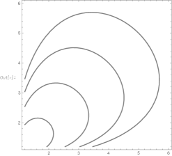
Figure 1: Contours of the peak height in the $(a,b)$-plain for the beta distribution $f(x;a,b)=x^{a-1}(1-x)^{b-1}/{\rm B}(a,b),x\in[0,1];a,b\geq 1$.

For discrete distributions the situation is radically different, since the peak of probability function need not be constant exactly, rather has some room to vary along the modal ridge, for instance to decay with $n$ as is the case for $S_{n}$ with binomial distribution, see Figure 2.

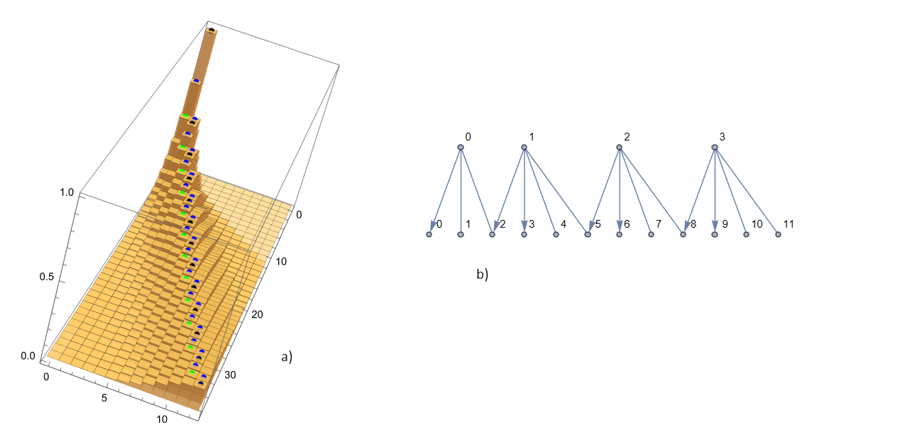
Figure 2: a) The modal ridge of the binomial distribution with $p=1/3$ and varying $n$. Blue and black spots mark the leading modes, black spots mark the larger likelihood maximiser. b) For this distribution, the bipartite graph of the modal correspondence: e.g. $m_{\pm}(8,1/3)=\{2,3\},\ell_{\pm}(2)=\{5,6\}$.

In this paper we focus on the modal properties of distributions representable as convolution of a Poisson distribution and any number (finite or infinite) of Bernoulli distributions with success probabilities that vary from trial to trial. Random variables with such distribution will be called here extended Bernoulli sums. This name echoes the term extended Poisson-binomial distribution suggested in Broderick et al [5]. In Madiman et al [19] the class of extended Bernoulli sums is introduced implicitly as a weak closure of the family of Poisson-binomial distributions.

The interest to independent Bernoulli trials with varying success probabilities $p_{1},p_{2},\ldots$ is rooted deeply in history. This sampling model was introduced by Poisson and was known as the Poisson scheme in earlier literature, but later the terminology was abandoned. The derived distribution of the number of successes $S_{n}$ is nowadays commonly called the Poisson-binomial distribution [29]. The first systematic study was undertaken in 1846 by Chebyshev [7], who established that amongst the Poisson-binomial distributions with given mean the expectation ${\mathbb{E}}[\varphi(S_{n})]$ is maximised by a shifted binomial distribution (his main result was only stated for the indicators needed to estimate the tail probabilities ${\mathbb{P}}[S_{n}\leq a]$ and ${\mathbb{P}}[S_{n}\geq b]$ but the argument covers the general case). About a century later Hoeffding [11] proved a more detailed theorem implying that the extremal property of the binomial distribution holds for $\varphi$ any convex function on integers. Bonferroni’s little known paper [3] was the first to observe the logconcavity of $S_{n}$, to analyse the behaviour of the peak as $n$ varies and to show that the difference between the mode and the mean is always $o(n)$. Apparently independentlly, the logconcavity was rediscovered soon thereafter by Lévy [17]. Darroch [9] and Samuels [26] found that the mode differs from the mean by no more than $1$, with the two being equal whenever the mean is an integer. Similar results for the median were shown in Jogdeo and Samuels [13]. Pollard [24] presents a detailed exposition of much of this development. Pitman [23] connected the results about the mode to bounds on coefficients of totally positive polynomials, giving many examples of combinatorial origin. The modal properties of $S_{n}$ were most thoroughly studied for the Karamata-Stirling profile of success probabilities $p_{i}=\theta/(\theta+i-1)$, especially in the case $\theta=1$, in connection with Stirling numbers, theory of records and random combinatorial structures, see Kabluchko et al [14] for recent results and references.

In the other direction, the statistical problem of estimating an unknown number of trials from the observed number of succeses calls to consider $n$ as a parameter. Assuming the success probabilities known, the unimodality of likelihood was first shown for $p_{i}=1/i$ by Moreno-Rebollo et al [21] and Cramer [8] then in general by Moreno-Rebollo et al [22]. In disguise, the fact also appeared in Bruss and Paindaveine [6] and Tamaki [28] in connection with versions of the famous secretary problem of optimal stopping.

The plan for the rest of the paper is the following. In Section 2 we give a thorough review of basic modal features of the Poisson and binomial distributions. In Section 3 we show that for the logconcave power series families the cross modality amounts to Darroch’s mean-mode rule. In Section 4 we introduce techniques to work with extended Bernoulli sums and apply these to the analysis of the peak height. Section 5 is devoted to the geometry of likelihood contours in the parameter space and presents an extension of Samuels [26] version of Darroch’s rule. In section 6 we prove the cross modality for certain monotonic (directed) families of extended Bernoulli sums, and give yet another proof of extended Darroch’s rule by deriving it from the the cross modality. In the last section 7 we address aspects of a mass transport problem for the extended Bernoulli sums, with the objective to shift the mode.

In the sequel we will be dealing with families of discrete distributions, with context-dependent range $R$ of a family being either $\{0,1,\ldots,n\}$ or $\{0,1,\ldots\}$.

2 The binomial and Poisson distributions

In this section we revise under the angle of cross modality the well known properties of the binomial and the Poisson distributions, also using this occasion to introduce notation and terminology. The connection between modes of the binomial and negative binomial distributions might have not been noticed in the literature.

For independent Bernoulli trials $B_{1},B_{2},\ldots$ with the same success probability $0<p<1$, let $S_{n}=B_{1}+\cdots+B_{n}$, $S_{0}=0$. The binomial distribution of $S_{n}$ has the probability function

$$f(k;n,p)={n\choose k}p^{k}(1-p)^{n-k},$$ (1)

which we extend by zero outside the support $\{0,1,\ldots,n\}$. The mode of this distribution is either a single integer or two adjacent integers (twins). The bifurcation of the mode can be neatly described by means of two functions $m_{-}(n,p)\leq m_{+}(n,p)$, where $m_{+}(n,p)$ is the leading mode determined as the unique integer $k$ satisfying the inequalities

$$f(k-1;n,p)\leq f(k;n,p)>f(k+1;n,p).$$ (2)

The second function $m_{-}(n,p)$ is defined by setting $m_{-}(n,p)=m_{+}(n,p)$ unless the first relation in (2) is equality in which case we set $m_{-}(n,p)=m_{+}(n,p)-1$. With this notation, the mode of the binomial distribution is $m(n,p)=[m_{-}(n,p),m_{+}(n,p)]$, either singleton or two-point integer interval. From the general perspective, the way of finding the mode via (2) relies on the logconcavity of distribution.

Explicitly from (1) and (2), $m_{+}(n,p)$ is the unique integer $k$ satisfying the inequalities

$$k\leq(n+1)p<k+1.$$ (3)

If $(n+1)p$ is not integer then $m_{\pm}(n,p)=\lfloor(n+1)p\rfloor$ is a sole mode of the distribution, and if $(n+1)p$ is a positive integer then the mode is twin $m(n,p)=[(n+1)p-1,(n+1)p]$.

To achieve solvability of the unconstrained likelihood maximisation problem we close the family of binomial distributions by allowing $p\in\{0,1\}$, and extend the definition of modal functions as $m_{\pm}(n,0)=0,m_{\pm}(n,1)=n$. With the range of the family being $R=\{0,1,\ldots\}$, the modal ridge can be identified as the set of triples $(k,n,p)$ where $k\in m(n,p),n\in\{0,1,\ldots\}$ and $p\in[0,1]$. The closed family is trivially cross modal, since for given $k$ the unique unconstrained likelihood maximiser is $(n,p)=(k,1)$ with $f(k;k,1)=1$.

We procede with discussing the cross modality for two standard subfamilies of binomial distributions, where the likelihood maximisers are genuine distributions.

2.1 The binomial-$n$ family

Suppose first that $0<p<1$ is fixed while $n$ varies, thus the likelihood becomes a function of the active parameter $n$. Let $T_{k}$ be the index of the $k$th success (with $T_{0}=0$). By the elementary identity

$${\mathbb{P}}[T_{k+1}=n+1]=p\,{\mathbb{P}}[S_{n}=k],$$

the likelihood function $f(k;\cdot,p)$ is just a multiple of the probability function of the random variable $T_{k+1}-1$, which has a Pascal distribution. The distribution of $T_{k}$ is the $k$th convolution power of the geometric distribution for $T_{1}$ hence logconcave with one or two modes. Similarly to (2) maximising the likelihood amounts to finding $\ell_{+}(n)$ as the unique $k$ satisfying

$$f(k;n-1,p)\leq f(k;n,p)>f(k;n+1,p),$$ (4)

then setting $\ell_{-}(n)=\ell_{+}(n)$ if the first relation in (4) is strict and $\ell_{-}(n)=\ell_{+}(n)-1$ in the case of equality. This leads to identifying $\ell_{+}(k)$ as the unique integer $n$ satisfying the inequalities

$$n\leq\frac{k}{p}<n+1$$ (5)

similar to (3). Explicitly, if $\frac{k}{p}$ is not a positive integer we have $\ell_{+}(n)=\ell_{-}(n)=\lfloor\frac{k}{p}\rfloor$, and if $\frac{k}{p}$ is a positive integer then $\ell_{+}(n)=\frac{k}{p}$ and $\ell_{-}(n)=\frac{k}{p}-1$.

With the above explicit formulas in hand, it is now easy to verify the crossmodality of the binomial sum $S_{n}$ relative to parameter $n$, in the form

$$n\in\{\ell_{\pm}(k)\}\Rightarrow k\in\{m_{\pm}(n)\},$$ (6)

meaning that if $n$ is a likelihood maximiser for some $k$, then $(k,n)$ is a cross mode.

Indeed, suppose first that $\frac{k}{p}$ is not integer, thus the inequalities for $n$ in (5) are strict: then $n=\ell_{\pm}(k)$ and noting that (5) gives $k<(n+1)p=np+p<np+1<k+1$ we obtain (3), whence $k=m_{\pm}(n,p)$. In the case $k=0$ we trivially have $m_{\pm}(0,p)=\ell_{\pm}(n)=0.$ In the remaining case of integer $n=kp$, we have that $n=\frac{k}{p}<n+1$ implies $\ell_{+}(k)=n$ and $\ell_{-}(k)=n=1$, that $k=np<k+1$ implies $m_{+}(n-1,p)=k$, and $m_{-}(n-1,p)=k=1$, and finally that $k<(n+1)p<k+1$ implies $m_{\pm}(n,p)=k$ as above. We conclude that $m_{-}(\ell_{-}(k),p)=k-1$ only holds if $\frac{k}{p}$ is a positive integer, while $m_{\pm}(\ell_{\pm}(k),p)=k$ holds in all other cases. See Figure 2.

Equivalently, if $np<k<(n+1)p$ the pattern of relations about the cross mode $(k,n)$ is

$${}_{\begin{array}[]{ccccc}&&f(k;n-1,p)&&\\ {}\hfil&{}\hfil&\mathrel{\rotatebox{90.0}{$>$}}&{}\hfil&{}\hfil\\ f(k-1;n,p)&<&f(k;n,p)&>&f(k+1;n,p)\\ &{}\hfil&\mathrel{\rotatebox{90.0}{$<$}}&{}\hfil&{}\hfil\\ &{}\hfil&f(k;n+1,p)&{}\hfil&{}\hfil\end{array}}$$ (7)

and if $k=(n+1)p$ the mode bifurcates and the pattern becomes

$${}_{\begin{array}[]{ccccc}&&f(k;n-1,p)&&\\ {}\hfil&{}\hfil&\mathrel{\rotatebox{90.0}{$>$}}&{}\hfil&{}\hfil\\ f(k-1;n,p)&=&f(k;n,p)&>&f(k+1;n,p)\\ &{}\hfil&\mathrel{\rotatebox{90.0}{$=$}}&{}\hfil&{}\hfil\\ &{}\hfil&f(k;n+1,p)&{}\hfil&{}\hfil\end{array}}$$ (8)

If $p$ is irrational number the mode does not bifurcate, hence only the strict pattern (7) occurs. If $p$ is rational, we may write $p=\frac{a}{b}$ with mutually prime integers $a<b$, and the triple equality in (7) simplifies as the elementary identity for binomial coefficients,

$${cb-1\choose ca-1}b(b-a)={cb-1\choose ca}ab={cb\choose ca}a(b-a).$$

Explicit formulas we used obscur the mechanics of cross modality, which becomes transparent by turning to the recursion

$$f(k;n+1,p)=pf(k-1;n,p)+(1-p)f(k;n,p),$$ (9)

that obtains by either conditioning $S_{n+1}$ on the outcome of one trial or, what is equivalent, by noting that adding to $S_{n}$ an independent Bernoulli variable yields $S_{n+1}$. Geometrically, the recursion means that the probability function of $S_{n+1}$ is a convex combination of the probability functions of $S_{n}$ and $S_{n}+1$, see Figure. If $m_{-}(n,p)=m_{+}(n,p)$, the shapes of distributions of $S_{n}$ and $S_{n+1}$ have discordant directions of strict monotonicity only within $[m_{+}(n,p),m_{+}(n,p)+1]$, and if $m_{-}(n,p)<m_{+}(n,p)$ then disagreement occurs within $[m_{+}(n,p)-1,m_{+}(n,p)+1]$ where one of the shapes is flat. It follows that the unimodality of $S_{n}$ implies that $S_{n+1}$ is unimodal with a lower peak, unless the mode of $S_{n}$ is twin in which case the peak remains the same and the new mode becomes $m_{\pm}(n+1,p)=m_{+}(n,p)>m_{-}(n,p)$. This way we connect the maximisers as

$$\ell_{-}(k)=\min\{n:m_{+}(n,p)=k\},$$ (10)

and observe that $f(k;n,p)$ strictly increases in $n$ as long as the leading mode does not hit $k$, then after possibly staying flat one step strictly decreases.

For the modal ridge we have therefore dual representations via the $n$- and $k$-sections as

$$M_{(\cdot,p)}=\bigcup\limits_{n=0}^{\infty}m(n,p)\times{\{n\}}=\bigcup_{k=0}^{\infty}\{k\}\times[\ell_{-}(k),\ell_{+}(k+1)-1].$$

2.2 The binomial-$p$ family

The second, more common setting, is where $n>0$ is fixed and $p$ varies. Let $\ell_{\circ}$ denote the likelihood maximiser relative to the ‘unknown $p$’ family of the binomial distributions. Equating the derivative

$$\partial_{p}f(k;n,p)=\frac{k-np}{p(1-p)}f(k;n,p)$$

to zero we find that the maximiser is single-valued and given by the textbook formula $\ell_{\circ}(k)=\frac{k}{n}$. The cross modality follows from the identity

$$m_{\pm}\left(n,\frac{k}{n}\right)=k,~{}~{}~{}0\leq k\leq n,$$

which is trivial for $k\in\{0,n\}$ and for $0<k<n$ is a specialisation of (3) as

$$k<(n+1)\frac{k}{n}<k+1.$$

The function $m_{+}(n,p)$ is right-continuous, having unit jumps at points $p_{k}=\frac{k}{n+1}$ that satisfy

$$f(k-1;n,p)=f(k;n,p),~{}0\leq k\leq n,$$

and can be also characterised as maximisers of $f(k+1;n,p)$ as is seen from the formula

$$\partial_{p}f(k;n+1,p)=f(k-1;n,p)-f(k;n,p),$$ (11)

derived from (9). For $p_{k}$ with $0<k<n$ the mode is twin. Note the interlacing pattern of pivot points

$$0=p_{0}=\ell_{\circ}(0)<p_{1}<\ell_{\circ}(1)<p_{2}<\cdots<\ell_{\circ}(n-1)<p_{n}<\ell_{\circ}(n)=1.$$

The cross modality comes forward as the following pattern: the likelihood function $f(k;p,n)$ increases in $p$ on $[0,p_{k}]$ until $k$ becomes a mode, then keeps growing until reaching the maximum at $\ell_{\circ}(k)$, then decays with the modal status lost at $p_{k+1}$. The modal ridge becomes (with $p_{n+1}:=1$)

$$M_{(n,\cdot)}=\bigcup_{k=0}^{n}\{k\}\times[p_{k},p_{k+1}],$$

2.3 The Poisson distribution

For the Poisson distribution

$$f(k;t)=e^{-t}\frac{t^{k}}{k!},~{}~{}~{}k\geq 0,$$

with parameter $t\geq 0$ the modal properties are similar to that of both binomial families. The pivotal values of the parameter are nonnegative integers $t_{k}=k$, whose role is twofold:

• $f(k;t_{k})=f(k-1;t_{k}),k\geq 1,$ hence the mode bifurcates, that is $m_{+}(t_{k})=m_{-}(t_{k})+1$, while $m_{+}(t)=m_{-}(t)=\lfloor t\rfloor$ for $t$ not a positive integer,

• $f(k;t)$ as the likelihood function coincides with the density of the Erlang distribution with shape parameter $k+1$, attaining its unique maximum at $t_{k}$.

The likelihood maximisers coincide with the bifurcation points, forcing the mean curve to cross the graph of the leading mode in the northwest corner points, see the plot in Figure 3.

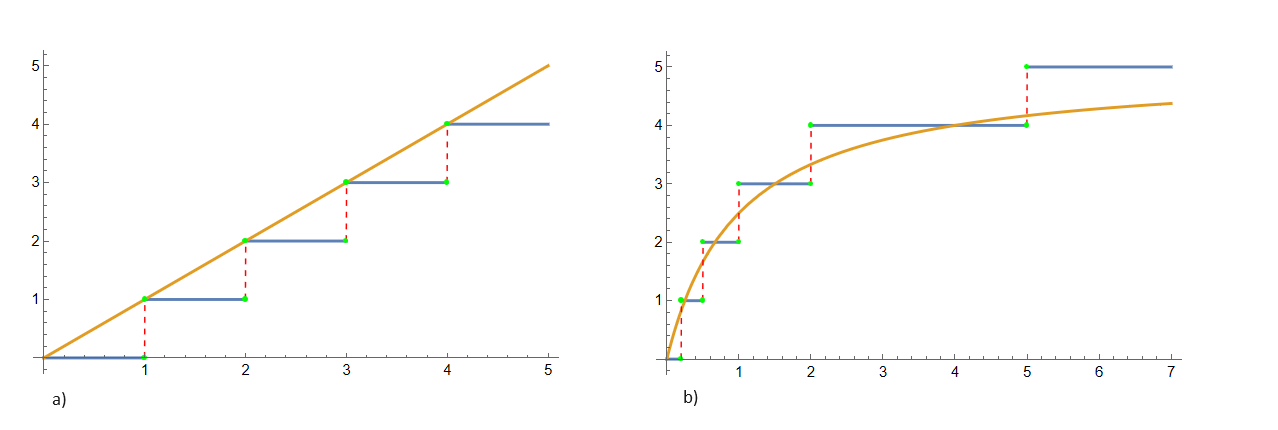
Figure 3: a) The mean and the mode curves for the Poisson distribution. b) Same for the binomial distribution with $n=5$ and parameter $t=p/(1-p)$.

The peak height $f(k;k)=e^{-k}\frac{k^{k}}{k!}$ is decreasing to $0$ with $k$.

3 Power series distributions

Every distribution on nonnegative integers can be included in one-parameter discrete exponential family, which can be conveniently represented by a power series with nonnegative coefficients. A nice feature of such a family is that the likelihood maximisation amounts to matching the mean with the observed value $k$. In the unimodal case this allows one to express the cross modality in a simple way described in this section.

Let $a_{0},a_{1},\ldots$ be a positive sequence such that the quotients of adjacent terms satisfy

$$\frac{a_{k+1}}{a_{k}}\downarrow 0~{}~{}{\rm as}~{}k\to\infty,$$

where the decrease is strict. By the ratio convergence test, the power series

$$F(t)=\sum_{k=0}^{\infty}a_{k}t^{k}$$

defines an entire function. The associated power series distribution has the form

$$f(k;t)=\frac{a_{k}t^{k}}{F(t)},~{}~{}~{}k\geq 0,$$ (12)

where $t\geq 0$ appears as a parameter. The probability generating function of (12) is

$$z\mapsto\sum_{k=0}^{\infty}f(k;t)z^{k}=\frac{F(tz)}{F(t)}.$$

The assumption on coefficients implies strict logconcavity $a_{k}^{2}>a_{k-1}a_{k+1}$ for $k\geq 1$, hence the distribution is unimodal and has all moments [16]. The general power series distribution strictly increases with $t$ in the stochastic order, because the tail probability $\sum_{j=1}^{\infty}f(k+j;t)$ increases in consequence of the fact that in the formula for the reciprocal

$$\frac{1}{\sum_{j=1}^{\infty}f(k+j;t)}=\frac{F(t)}{\sum_{j=1}^{\infty}a_{k+j}t^{k+j}}=1+\sum_{i=0}^{k}\frac{a_{i}}{\sum_{j=1}^{\infty}a_{k+j}t^{k+j-i}}$$

the terms of the external sum are decreasing to $0$. Therefore the limit distribution is the delta mass at $\infty$ as $t\to\infty$, and the mean

$$\mu(t)=t\,\partial_{t}\log F(t)$$

is a smooth, strictly increasing function with $\mu(0)=0$ and $\mu(t)\uparrow\infty$.

The likelihood quotient

$$\frac{f(k;t)}{f(k-1;t)}=\frac{a_{k}\,t}{a_{k-1}},~{}~{}~{}k\geq 1,$$

is increasing in both $k$ and $t$, and equals $1$ at point

$$t_{k}:=\frac{a_{k-1}}{a_{k}},~{}~{}~{}k\geq 1,$$

which is a unique solution to $f(k-1;t)=f(k,t)$. It is readily seen that $t_{k}\uparrow\infty$ (strictly, with $t_{0}:=0$), and that the leading mode $m_{+}(t)$ is right-continuous, nondecreasing, takes value $k$ on the interval $[t_{k-1},t_{k}]$ and bifurcates at the point $t_{k}$, where it has a unit jump for $k>0$ (that is, $m_{-}(t_{k})=k-1$)).

We assert that for each $k$ the likelihood has a single maximum point $\ell(k)$, which coincides with the (unique) solution to the equation $\mu(t)=k$. Indeed, the likelihood is zero at $t\in\{0,\infty\}$, and the loglikelihood satisfies $t\,\partial_{t}\log f(t;k)=k-\mu(t)$ by easy calculus.

Proposition 1

The family of logconcave power series distributions (12) is cross modal if and only if whenever $\mu(t)$ is integer it coincides with a mode. This condition is equivalent to any of the following three conditions:

• $t_{k}\leq\ell(k)\leq t_{k+1},~{}~{}k\geq 1$,

• $k-1\leq\mu(t_{k})\leq k,~{}~{}k\geq 1$,

• $\sup|\mu(t)-m_{+}(t)|\leq 1$.

Proof. For cross modality $k$ must be a mode of $f(\cdot;\ell(k))$, which is (i) since $k$ is a mode for $t\in[t_{k-1},t_{k}]$. The rest of proposition follows from the identification of $\ell(k)$ as the root of $\mu(t)=k$, combined with the continuity and monotonicity properties of $m_{+}(t)$ and $\mu(t)$. $\Box$

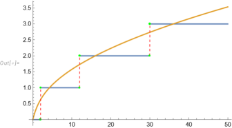
Figure 4: The mean and the mode functions for the power series distribution derived from $F(t)=\cosh\sqrt{t}$.

Explicitly, condition (ii) becomes

$$(k-1)\sum_{j=0}^{\infty}a_{j}\left(\frac{a_{k-1}}{a_{k}}\right)^{j}\leq\sum_{j=1}^{\infty}ja_{j}\left(\frac{a_{k-1}}{a_{k}}\right)^{j}\leq k\sum_{j=0}^{\infty}a_{j}\left(\frac{a_{k-1}}{a_{k}}\right)^{j}.$$ (13)

Since the Poisson distribution is the edge case, with $\ell(t_{k})=\mu(t_{k})=t_{k}=k$ and the second relation in (13) being equality, one can hope that the ultra logconcavity

$$\frac{a_{k}}{a_{k+1}}\frac{1}{k+1}\geq\frac{a_{k-1}}{a_{k}}\frac{1}{k}$$

would be sufficient for the cross modality. Unfortunately, this does not materialise. For, denote the right-hand side $b_{k}:=a_{k-1}/(ka_{k})$; these parameters are now only constrained by the monotonicity $0<b_{1}\leq b_{2}\leq\ldots$ Manipulating the second inequality in (13) we reduce it to the condition

$$\sum_{j=0}^{\infty}\frac{b_{k}^{j}}{b_{1}\cdots b_{j}}\frac{k^{j}}{j!}\left(1-\frac{b_{k}}{b_{j+1}}\right)\geq 0.$$

But for $k>1$ and any given $b_{k},b_{k+1},\ldots$ we may choose $b_{1}<\ldots<b_{k-1}$ sufficiently small to have the whole infinite sum negative.

A finite positive sequence $a_{0},\ldots,a_{n}$ seen as coefficients of the polynomial $F(t)=\sum_{k=1}^{n}a_{k}t^{k}$ induces a family of distributions supported by $\{0,1,\ldots,n\}$. The definitions and findings of this section are easily adjusted to the polynomial case. In this framework the largest bifurcation point is $t_{n}=a_{n-1}/a_{n}$ for polynomial of degree $n$, and the mean satisfies $\mu(t)\uparrow n$, so it is logical to set $\ell(n)=\infty$. The binomial-$p$ family fits in the scheme by the re-parametrisation $t=p/(1-p)$, see Figure 3. Pitman [23] argues in the direction opposite to ours, observing that the mean-mode relations imply bounds on the quotients $a_{k-1}/a_{k}$.

4 Extended binomial sums

4.1 Definitions and construction

Given $\lambda\geq 0$ and a profile of success probabilities ${\boldsymbol{p}}=(p_{1},p_{2},\ldots)$ with $\sum_{i=1}^{\infty}p_{i}<\infty$, the extended Bernoulli sum is a random variable $S=X+\sum_{i=1}^{\infty}B_{i},$ where $X\stackrel{{\scriptstyle d}}{{=}}{\rm Poisson}(\lambda)$ and $B_{i}\stackrel{{\scriptstyle d}}{{=}}{\rm Bernoulli}(p_{i})$ are jointly independent. The probability function of $S$, written as $f(k;\lambda,\boldsymbol{p}),~{}k\geq 0$, depends symmetrically on the $p_{i}$’s, so the uniqueness of parametrisation is achieved by relating each distribution to a point of the infinite-dimensional convex set $\nabla:=\{(\lambda,\boldsymbol{p}):\lambda\geq 0~{}{\rm and~{}}1\geq p_{1}\geq p_{2}\geq\ldots\geq 0)$, which has the natural component-wise partial order. The mean of $S$ will be denoted

$$\mu(\lambda,\boldsymbol{p}):=\sum_{k=0}^{\infty}kf(k;\lambda,\boldsymbol{p})=\lambda+\sum_{i=1}^{\infty}p_{i}.$$

Note that $\mu(\lambda,\boldsymbol{p})$ is the $l_{1}$-norm, and whenever $(\lambda_{1},\boldsymbol{p}_{1})\geq(\lambda_{2},\boldsymbol{p}_{2})$ the difference $\mu(\lambda_{1},\boldsymbol{p}_{1})-\mu(\lambda_{2},\boldsymbol{p}_{2})$ equals the $l_{1}$-distance between the vectors $(\lambda_{1},\boldsymbol{p}_{1})$ and $(\lambda_{2},\boldsymbol{p}_{2})$.

We endow $\nabla$ with the topology in which convergence amounts to the convergence in distribution of the corresponding extended Bernoulli sums (that is, pointwise convergence of the $f(\cdot;\lambda,\boldsymbol{p})$’s). Explicitly, convergence of a sequence $\{(\lambda_{j},\boldsymbol{p}_{j})\}\subset\nabla$ in this topology amounts to the componentwise convergence of $\boldsymbol{p}_{j}$’s and convergence of the mean values $\mu(\lambda_{j},\boldsymbol{p}_{j})$, with the behaviour of $\lambda_{j}$’s being subordinate to these rules. In particular, the familiar convergence of Bernoulli convolutions to a Poisson distribution in terms of the parameters is equivalent to $(0,\boldsymbol{p}_{j})\to(\lambda,{\boldsymbol{0}})$, which holds when $\boldsymbol{p}_{j}\to{\boldsymbol{0}}$ (this is equivalent to the convergence of the largest term to $0$) and $\mu(0,\boldsymbol{p}_{j})\to\lambda$. To illustrate, convergence of the binomial distribution to Poisson corresponds to the relation

$$(0,\underbrace{\lambda/n,\ldots,\lambda/n}_{n~{}{\rm times}},0,0,\ldots)\to(\lambda,0,0,\ldots).$$

By the alternative parametrisation by $\mu$ and ordered and ordered $\boldsymbol{p}$ satisfying $\mu\geq\sum_{i=1}^{\infty}p_{i}$, the adopted topology becomes the product topology. Broderick et al [5] use discrete measures $\lambda\delta_{0}+\sum_{i=1}^{\infty}p_{i}\delta_{p_{i}}$ to encode the parameters, but the vector representation has the advantage that the Bernoulli terms get naturally labelled. The uniqueness of parametrisation by $\nabla$ is a part of a more general result on totally positive sequences [15]. See [5] for a more probabilistic proof.

The finitary Poisson-binomial distributions with $n$ Bernoulli terms (some of which could be $0$) correspond to a compact face $\nabla_{n}\subset\nabla$ with points of the form $(0,p_{1},\ldots,p_{n},0,0,\ldots)$. The union $\cup_{n}\nabla_{n}$ is dense in $\nabla$, therefore many structural properties of the extended Poisson-binomial distribution can be concluded from their finitary counterparts but we prefer to avoid such way of reason, giving direct proofs whenever possible.

A simple randomisation device allows one to organise all extended Bernoulli sums in a infinite-parameter counting process $(S(\lambda,\boldsymbol{p}),~{}(\lambda,\boldsymbol{p})\in{\mathbb{R}}_{+}\times[0,1])$, where we do not restrict $\boldsymbol{p}$ to have the components $p_{i}$ nondecreasing. To that end, let $(N(\lambda),\lambda\geq 0)$ be a unit rate Poisson process, independent of i.i.d. random variables $U_{1},U_{2},\ldots$ with uniform distribution on $[0,1]$; this data can be regarded as a point process on the ground space ${\mathbb{R}}_{+}\cup(\cup_{i=1}^{\infty}[0,1])$. Setting $S(\lambda,\boldsymbol{p})=N(\lambda)+\sum_{i=1}^{\infty}1(U_{i}\leq p_{i})$ we obtain an integer-valued process with desired marginal distributions and paths nondecreasing in $(\lambda,\boldsymbol{p})$. Then $S(\lambda,\boldsymbol{p})$ is almost surely finite if $\mu(\lambda,\boldsymbol{p})<\infty$.

In the sequel, unless explicitly required, we will not restrict $p_{i}$’s to be nondecreasing. This freedom is needed to avoid re-labelling while allowing a particular success probability parameter to vary within the full range $[0,1$.

Sometimes it is convenient to use a parallel set of parameters $\boldsymbol{r}=(r_{1},r_{2},\ldots)$ for the Bernoulli variables with the largest $p_{1}<1$, where $r_{i}$ is interpreted as odds in favour of success, and the connection is

$$r_{i}:=\frac{p_{i}}{1-p_{i}}\Longleftrightarrow p_{i}=\frac{r_{i}}{1+r_{i}}.$$

Clearly, $\sum_{i}r_{i}<\infty$ is equivalent to $\sum_{i}p_{i}<\infty$ if $p_{1}<1$.

The probability generating function of $S$ is an entire function with only negative zeros,

$$G(z)=G(0)\,e^{\lambda z}\prod_{i=1}^{\infty}(1+r_{i}z),~{}~{}{\rm where}~{}~{}G(0)=e^{-\lambda}\prod_{i=1}^{\infty}(1-p_{i})=e^{-\lambda}\prod_{i=1}^{\infty}\frac{1}{1+r_{i}}.$$ (14)

For $k=0,1,\ldots$ consider the elementary symmetric functions in the odds

$$E_{k}(0,\boldsymbol{r}):=\sum_{i_{1}<\cdots<i_{k}}r_{i_{1}}\cdots r_{i_{k}},$$

and let us introduce their extended counterparts

$$E_{k}(\lambda,\boldsymbol{r}):=\sum_{j=0}^{k}\frac{\lambda^{k-j}}{(k-j)!}E_{j}(0,\boldsymbol{r}).$$

The convergence of the multiple series is ensured by the summability of $r_{i}$’s and can be concluded by expressing the elementary symmetric functions as polynomials in Newton’s power sums $\sum_{i}r_{i}^{n}$. In this notation, the probability function of $S$ becomes

$$f(0;\lambda,\boldsymbol{p})=S(0),~{}~{}~{}f(k;\lambda,\boldsymbol{p})=f(0;\lambda,\boldsymbol{p})E_{k}(\lambda,\boldsymbol{r}).$$

We extend this by zero, setting $f(-k;\lambda,\boldsymbol{p})=E(-k;\lambda,\boldsymbol{p})=0$ for $k>0$.

Throughout $f(k;\lambda,\boldsymbol{p}\setminus p_{i})$ will denote the probability of $k$ successes with the $i$th Bernoulli trial ignored (this is the probability function of $S-B_{i}$), and $E_{k}(\lambda,\boldsymbol{r}\setminus r_{i})$ will denote the symmetric function with variable $r_{i}$ set to zero. Reciprocally, the convolution with yet another independent Bernoulli$(p)$ variable is denoted $f(k;\lambda,\boldsymbol{p}\cup p)$. Similar notation will apply to the operations of removing or adding two or more independent Bernoulli variables. The operator $\Delta$ will act in the variable $k$ as forward difference $\Delta f(k)=f(k+1)-f(k)$.

The following lemma summarises some of the properties of the probability function.

Lemma 1

The probability function of the extended Bernoulli sum satisfies:

• $f(k;\lambda,\boldsymbol{p})=p_{i}f(k-1;\lambda,\boldsymbol{p}\setminus p_{i})+(1-p_{i})f(k;\lambda,\boldsymbol{p}\setminus p_{i}),$

• (ultra log-concavity) for $k\geq 1$

  $${kf^{2}(k;\lambda,\boldsymbol{p})}\geq{(k+1){f(k-1;\lambda,\boldsymbol{p})}f(k+1;\lambda,\boldsymbol{p})},$$

  where the inequality is strict unless $\boldsymbol{p}=0$, or $\lambda=0$ and there are less than $k$ positive $p_{i}$’s (when both sides are zero),

• (linearity in $p_{i}$)

  $$\partial_{p_{i}}f(k;\lambda,\boldsymbol{p})=-\Delta f(k-1;\lambda,\boldsymbol{p}\setminus p_{i}),$$

• $\partial_{\lambda}f(k;\lambda,\boldsymbol{p})=-\Delta f(k-1;\lambda,\boldsymbol{p}),$

• (monotone likelihood ratio)

  $$\partial_{p_{i}}\frac{f(k+1;\lambda,\boldsymbol{p})}{f(k;\lambda,\boldsymbol{p})}>0,~{}~{}~{}\partial_{\lambda}\frac{f(k+1;\lambda,\boldsymbol{p})}{f(k;\lambda,\boldsymbol{p})}>0,$$

• $kf(k;\lambda,\boldsymbol{p})=\sum_{i=1}^{\infty}p_{i}f(k;\lambda,\boldsymbol{p}\setminus p_{i})+\lambda f(k-1;\lambda,\boldsymbol{p}).$

• (concave likelihood ratio)

  $$\frac{f(k+1;\lambda,\boldsymbol{p})}{f(k;\lambda,\boldsymbol{p})}$$

  is concave in $(\lambda,\boldsymbol{p})$, and strictly concave for $k>0$.

• for $d\geq 1$ and pairwise distinct $i_{1},\ldots,i_{d}$

  $$\partial^{d}_{p_{i_{1}},\ldots,p_{i_{d}}}f(k;\lambda,\boldsymbol{p})=(-\Delta)^{d}f(k-d;\lambda,\boldsymbol{p}\setminus p_{i_{1}},\ldots,p_{i_{d}}).$$

Proof. Assertion (i) follows by the total probability rule, which in terms of the symmetric functions becomes the recursion

$$E_{k}(\lambda,\boldsymbol{r})=r_{i}E_{k-1}(\lambda,\boldsymbol{r}\setminus r_{i})+E_{k}(\lambda,\boldsymbol{r}\setminus r_{i}).$$

Formula (iii) follows straight from (i).

Part (ii) for $\boldsymbol{p}=0$ is an easy factorial identity. For some number $n\geq k$ of nonzero $p_{i}$’s, matching powers of $\lambda$ and applying Newton’s inequality yields a stronger inequality. The case with infinitely many positive $p_{i}$’s is treated by induction in $k$ using (i). The claim also follows by checking the property for Poisson and Bernoulli distributions, and applying Liggett’s theorem [18] which asserts that the ultra log-concavity is preserved by convolution, Saumard and Wellner [30] give a detailed discussion, including the interpretation of ultra-logconcavity as the log-concavity relative to the Poisson distribution.

Part (iv) is straight from $\partial_{\lambda}f(0;\lambda,\boldsymbol{p})=-f(0;\lambda,\boldsymbol{p})$ and $\partial_{\lambda}E_{k}(\lambda,\boldsymbol{r})=E_{k-1}(\lambda,\boldsymbol{r})$.

For (v), using $\partial_{p_{i}}r_{i}>0$ we are reduced to checking the analogue in terms of the odds, which is the inequality $\partial_{r_{i}}[E_{k+1}(\lambda,\boldsymbol{r})/E_{k}(\lambda,\boldsymbol{r})]>0.$ Differentiating the quotient, after simplification of the numerator the inequality follows from log-concavity.

The identity (vi) was stated in [26] for the finitary case without proof. To show (vi), write the desired identity in terms of the odds,

$$kE_{k}(\lambda,\boldsymbol{r})=\sum_{i=1}^{\infty}r_{i}E_{k}(\lambda,\boldsymbol{r}\setminus r_{i})+\lambda E_{k-1}(\lambda,\boldsymbol{r}).$$

The formula is proved by differentiating the homogeneity identity $E_{k}(z\lambda,z\boldsymbol{r})=z^{k}E_{k}(\lambda,\boldsymbol{r})$ in $z>0$, using the above formulas for partial derivatives, and setting $z=1$.

(vii) Passing to the quotient of $E_{k}(\lambda,\boldsymbol{r})$’s this is shown as in [20], p. 116.

(viii) Obtained by iterating (i) or (iii).

$\Box$

A number of other classical inequalities for symmetric polynomials [20] that do not restrict the number of variables have their extended analogues and can be interpreted as features of the probability function $f(k;\lambda,\boldsymbol{p})$.

By the log-concavity we can define the leading mode $m_{+}(\lambda,\boldsymbol{p})$ to be the unique integer $k$ satisfying

$$f(k-1,\lambda,\boldsymbol{p})\leq f(k,\lambda,\boldsymbol{p})>f(k+1,\lambda,\boldsymbol{p}),$$

and define $m_{-}(\lambda,\boldsymbol{p})$ as in the case of the binomial distribution. The probability function strictly increases for $k<m_{-}(\lambda,\boldsymbol{p})$ and strictly decreases for $k\geq m_{+}(\lambda,\boldsymbol{p})$ (unless turning zero in the finitary case). If $m_{-}(\lambda,\boldsymbol{p})=m_{+}(\lambda,\boldsymbol{p})$ the mode is singleton, and if $m_{-}(\lambda,\boldsymbol{p})+1=m_{+}(\lambda,\boldsymbol{p})$ the mode is twin. Thus, the mode is identified by the equivalences

$$f(k-1;\lambda,\boldsymbol{p})<f(k;\lambda,\boldsymbol{p}) \Longleftrightarrow m_{-}(\lambda,\boldsymbol{p})\geq k,$$ (15)

$$f(k;\lambda,\boldsymbol{p})>f(k+1;\lambda,\boldsymbol{p}) \Longleftrightarrow m_{+}(\lambda,\boldsymbol{p})\leq k.$$ (16)

The peak height of the distribution $h(\lambda,\boldsymbol{p}):=\max_{k}f(k;\lambda,\boldsymbol{p})$ is attained at both $m_{+}(\lambda,\boldsymbol{p})$ and $m_{-}(\lambda,\boldsymbol{p})$ even when they are distinct, but only the leading mode $m_{+}(\lambda,\boldsymbol{p})$ is stable under small increase of the parameters.

4.2 The peak height

The peak height is a decreasing function of $\lambda$, that is $\partial_{\lambda}h(\lambda,\boldsymbol{p})\leq 0$ where $0$ only occurs if the mode at $(\lambda,\boldsymbol{p})$ is twin. We move on to revealing a more involved dependence of the peak on the $p_{i}$’s.

To start with, recall the discussion around (9) for the binomial distribution. Similarly to that, we may conclude on the unimodality of $S$ straight from the recursion (i) in Lemma 1, first using induction in the number of Bernoulli components for finitary distributions, then passing to limit. The key step is the following. Fix $(\lambda,\boldsymbol{p})$, and suppose yet another independent Bernoulli variable $B$ is added to $S$. Thus we have as in (9)

$$f(k;\lambda,{\boldsymbol{p}}\cup p)=p\,f(k-1;\lambda,{\boldsymbol{p}})+(1-p)f(k;\lambda,{\boldsymbol{p}}),$$ (17)

where the right-hand side is to be understood as a convex combination of probability function and its unit shift. The shapes in Figure 5 should convince the reader that the unimodality of $f(k;\lambda,{\boldsymbol{p}}\cup p)$ follows from that of $f(k;\lambda,{\boldsymbol{p}})$.

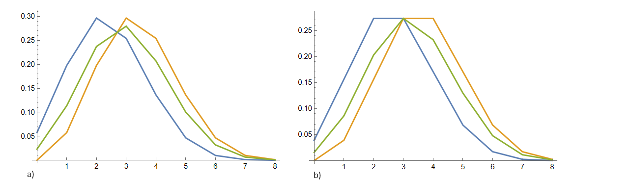
Figure 5: a) Evolution of single mode by adding a Bernoulli variable. b) Same for twin.

A quick look at Figure 5 shows that the shapes of (linearly interpolated) probability functions in (17) have a sole crossing point, which does not depend on $p$. Write for shorthand $m_{+}$ for the leading mode, and $f(m_{+}-1),f(m_{+}),f(m_{+}+1)$ for the values of $f(\cdot;\lambda,{\boldsymbol{p}})$ at these positions. The height of the crossing point is computed as

$$\frac{f^{2}(m_{+})-f(m_{+}-1)f(m_{+}+1)}{2f(m_{+})-f(m_{+}-1)-fm_{+}+1)}.$$

The peak height of $f(\cdot\,;\lambda,{\boldsymbol{p}}\cup p)$ will be at this level if $p$ is equal to the quantity

$$\gamma^{*}(\lambda,\boldsymbol{p}):=\frac{-\Delta f(m_{+})}{\Delta^{2}f(m_{+}-1)}\,,$$

which we will call the peak skewness (not to be confused with distribution skewness). A similar characteristic of the peak called ‘ratio’ was introduced in Baker and Handelman [2]. The leading mode of $S+B$ is $m_{+}$ if $p<\gamma^{*}(\lambda,\boldsymbol{p})$ and switches to $m_{+}$ if $p\geq\gamma^{*}(\lambda,\boldsymbol{p})$. Peak skewness $1$ only occurs if the mode of $S$ is twin, while peak skewness $1/2$ means that the distribution is symmetric near the mode. The peak height of $S+B$ obtains as

$$h(\lambda,\boldsymbol{p}\cup p)=\begin{cases}(1-p)f(m_{+})+pf(m_{+}+1),~{}~{}~{}{\rm if~{}}p>\gamma^{*}(\lambda,\boldsymbol{p}),\\ (1-p)f(m_{+})+pf(m_{+}-1),~{}~{}~{}{\rm if~{}}p<\gamma^{*}(\lambda,\boldsymbol{p}),\\ f(m_{+}),~{}~{}~{}{\rm if~{}}p=\gamma^{*}(\lambda,\boldsymbol{p}).\end{cases}$$

If the mode of $S$ is twin, the peak height of $S+B$ is the same as for $S$ regardless of $p$.

The above analysis of the effect from adding a Bernoulli variable readily tells us what happens when a variable gets removed from the extended Bernoulli sum.

Theorem 1

Both $m_{+}(\lambda,\boldsymbol{p})$ and $m_{-}(\lambda,\boldsymbol{p})$ are nondecreasing functions of the parameters, with the following connection to the monotonicity of the peak. The peak height function is differentiable in $\lambda$ and every $p_{i}$ and for $k=m_{+}(\lambda,\boldsymbol{p})$ we have

• $\partial_{p_{i}}h(\lambda,\boldsymbol{p})>0$ iff $m_{+}(\lambda,\boldsymbol{p}\setminus p_{i})=m_{-}(\lambda,\boldsymbol{p}\setminus p_{i})=k-1,$ in which case replacing $p_{i}$ in $\boldsymbol{p}$ by any larger value $p_{i}+\delta$ cannot switch the leading mode to $k+1$,

• $\partial_{p_{i}}h(\lambda,\boldsymbol{p})<0$ iff $m_{+}(\lambda,\boldsymbol{p}\setminus p_{i})=m_{-}(\lambda,\boldsymbol{p}\setminus p_{i})=k,$ in which case replacing $p_{i}$ in $\boldsymbol{p}$ by certain larger value $p_{i}+\delta$ will switch the leading mode to $k+1$,

• $\partial_{p_{i}}h(\lambda,\boldsymbol{p})=0$ iff $m_{+}(\lambda,\boldsymbol{p}\setminus p_{i})=m_{-}(\lambda,\boldsymbol{p}\setminus p_{i})+1=k,$ in which case replacing $p_{i}$ in $\boldsymbol{p}$ by any larger value $p_{i}+\delta$ will leave the single mode at $k$.

• $\partial_{\lambda}h(\lambda,\boldsymbol{p})\leq 0.$

Proof. We have seen that manipulating $p_{i}$ alone results in two possibilities for the mode, depending on how $p_{i}$ compares to the peak skewness of $f(\cdot;\lambda,\boldsymbol{p}\setminus p_{i})$. For instance, in case (i) replacing $p_{i}$ by $0$ moves the mode to $k=1$, hence $k+1$ cannot be achieved by replacing $p_{i}$ with $p_{i}+\delta$. The sign of $\partial_{p_{i}}h(\lambda,\boldsymbol{p})$ reads from Lemma 1(iii) specialised for $k$ the modal value. Part (iv) follows from Lemma 1 (iv). $\Box$

Whenever different monotonicity directions in (i) and (ii) occur the peak heaight function has a saddle point.

5 Geometry of the Darroch rule

5.1 The Poisson-binomial case

Darroch’s [9] rule localises the mode of the Poisson-binomial distribution in terms of the mean $\mu$. The rule states that whenever the mean is integer it coincides with a single mode, and if the mean is not a positive integer then the mode could be singleton $\lfloor\mu\rfloor$ or $\lceil\mu\rceil$ , or twin $\{\lfloor\mu\rfloor,\lceil\mu\rceil\}.$ Samuels [26] has noticed that the probability function is increasing for $k\leq\mu$ and decreasing for $k\geq\mu$.

A loose intuition suggesting that the mode and the mean are not far away from one another appears by looking at two extremes. If a Bernoulli variable with success probability zero or one is added to $S$ the mean and the mode both increment by zero or one, respectively. It will take some effort to make this idea work.

We give a geometric interpretation to the rule first in the finitary case. Consider the $n$-dimensional simplex $\nabla_{n}\subset\nabla$ whose points are the vectors of parameters $(0,p_{1},\ldots,p_{n},0,0,\ldots)$, where $1\geq p_{1}\geq\ldots\geq p_{n}\geq 0$. (The first zero in this notation stays for $\lambda=0$.) The apex of $\nabla_{n}$ is at $(0,{\boldsymbol{0}})$ and the simplex itself is a cap of a lattice cone. Let

$${\cal F}_{k,n} = \{(0,\boldsymbol{p})\in\nabla_{n}:f(k-1;0,\boldsymbol{p})=f(k;0,\boldsymbol{p})\},~{}k\geq 0,$$

$${\cal M}_{x,n} = \{(0,\boldsymbol{p})\in\nabla_{n}:\mu(0,\boldsymbol{p})=x\},~{}x\geq 0.$$

For $0<k\leq n$, ${\cal F}_{k,n}$ is a $(n-1)$-dimensional algebraic manifold (with boundary) which can be regarded as a section splitting $\nabla_{n}$ in two connected components. For $0<x<n$, ${\cal M}_{x,n}$ is a section of $\nabla_{n}$ by a hyperplane. For integer $0<k<n$ the set ${\cal M}_{k,n}$ is a $(n-1)$ dimensional simplex, for instance ${\cal M}_{2,3}$ is a triangle with extreme points

$$(0,1,1,0,0,\ldots),(0,1,\tfrac{1}{2},\tfrac{1}{2},0,\ldots),(0,\tfrac{2}{3},\tfrac{2}{3},\tfrac{2}{3},0,0,\ldots).$$

The ${\cal F}_{k,n}$’s for $0\leq k\leq n$ are pairwise disjoint in accord with the fact that no three positive values of the Poisson-binomial probability function can be equal.

By Darroch’s rule the manifolds arranged in the interlacing sequence

$${\cal F}_{1,n},{\cal M}_{1,n},{\cal F}_{2,n},\ldots,{\cal M}_{n-1,n},{\cal F}_{n,n}$$

are pairwise disjoint, as they are separated in terms of the $l_{1}$-norm $\mu(0,\boldsymbol{p})$, see Figure 6. For two neighbours in the sequence we may identify pairs of their points most close and most distant in the $l_{1}$-metric. Explicitly, the unique pair

$$(0,\underbrace{1,\ldots,1}_{k-1},\underbrace{\frac{1}{n-k+2},\ldots,\frac{1}{n-k+2}}_{n-k+1},0,0,\ldots) \in {\cal F}_{k,n},$$

$$(0,\underbrace{1,\ldots,1}_{k-1},\underbrace{\frac{1}{n-k+1},\ldots,\frac{1}{n-k+1}}_{n-k+1},0,0,\ldots) \in {\cal M}_{k,n}$$

realises the largest $l_{1}$-distance between the sets, which is equal to $1-\frac{n-k+1}{n-k+2}$. Likewise, the unique pair

$$(0,\underbrace{\frac{k}{k+1},\ldots,\frac{k}{k+1}}_{k},0,0,\ldots) \in {\cal F}_{k,n},$$

$$(0,\underbrace{1,\ldots,1}_{k},0,0,\ldots) \in {\cal M}_{k,n}$$

realises the smallest $l_{1}$-distance between the sets, which is equal to $1-\frac{1}{k+1}$. This can be verified using Chebyshev’s [7] device that the extreme values of $f(k;0,\boldsymbol{p})-f(k-1;0,\boldsymbol{p})$ on ${\cal M}_{x,n}$ are attained at some shifted binomial probability functions. An alternative approach is to reduce to a nonlinear programming problem with concave functions $f(k)/f(k-1)$ (Lemma 1 (vii)) and concave $\mu$ all expressed in the odds variables. It follows that for $0<k\leq n$ and $x$ in the bounds

$$k-1+\frac{1}{k+1}=\min_{{\cal F}_{k,n}}\mu(0,\boldsymbol{p})<x<\max_{{\cal F}_{k,n}}\mu(0,\boldsymbol{p})=k-\frac{1}{n-k+2}\,,$$ (18)

for $\boldsymbol{p}\in{\cal M}_{x,n}$ the mode could be any of $k,k-1,\{k-1,k\}$ and each possibility materialises. This leaves us for $0\leq k\leq n$ with the definite region

$$k-\frac{1}{n-k+2}<\mu(0,\boldsymbol{p})<k+\frac{1}{k+2} \Longrightarrow m(0,\boldsymbol{p})=\{k\},$$

$$\mu(0,\boldsymbol{p})=k-\frac{1}{n-k+2} \Longrightarrow m(0,\boldsymbol{p})=\{k-1,k\},$$

$$\mu(0,\boldsymbol{p})=k+\frac{1}{k+2} \Longrightarrow m(0,\boldsymbol{p})=\{k,k+1\},$$ (19)

which together with the assertion of ambiguity for the complementary region (18) constute a more detailed version of Darroch’s rule.

5.2 The extended binomial sums

We turn next to the extended binomial sums. Introduce

$${\cal F}_{k} = \{(\lambda,\boldsymbol{p})\in\nabla:f(k-1;\lambda,\boldsymbol{p})=f(k;\lambda,\boldsymbol{p})\},~{}k\geq 0,$$

$${\cal M}_{x} = \{(\lambda,\boldsymbol{p})\in\nabla:\mu(\lambda,\boldsymbol{p})=x\},~{}x\geq 0.$$

Similarly to the finitary case, the ${\cal F}_{k}$’s, $k\geq 0$, are pairwise disjoint closed sets (‘algebraic manifolds of codimension one’), and the ${\cal M}_{x}$’s, $x\geq 0$, are pairwise disjoint convex closed sets. By the definition we have

$${\cal F}_{k,n}={\cal F}_{k}\cap\nabla_{n},~{}~{}~{}{\cal M}_{k,n}={\cal M}_{k}\cap\nabla_{n},$$

which suggests that an infinite counterpart of Darroch’s rule could be obtained by an approximation argument. This is true and not hard to pursue for the main part of Darroch’s rule, thus showing that $|\mu(\lambda,\boldsymbol{p})-m_{\pm}(\lambda,\boldsymbol{p})|\leq 1$ holds in consequence of the chain of inequalities

$$\ldots<\min_{{\cal F}_{k}}\mu(\lambda,\boldsymbol{p})=k-1+\frac{1}{k+1}<k=\max_{{\cal F}_{k}}\mu(\lambda,\boldsymbol{p})<\ldots$$

In particular, we obtain $\max_{{\cal F}_{k}}\mu(\lambda,\boldsymbol{p})=k$ by sending $n\to 0$ in (19) and (18). But this implies existence of bifurcation points on ${\cal M}_{k}$ that need to be explicitly found. Indeed, from the Poisson$(k)$ case we know that $(k,{\boldsymbol{0}})\in{\cal M}_{k}\cap{\cal F}_{k}$ is one such point.

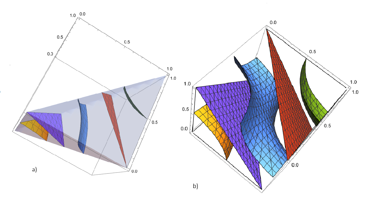
Figure 6: For $n=3$ surfaces $f(0)=f(1),\mu=1,f(1)=f(2),\mu=2$ and $f(2)=f(3)$ in a) simplex $\nabla_{3}$, and b) cube $[0,1]^{3}$. Shorthand notation: $f(k)=f(k;0,p_{1},p_{2},p_{3},0,0,\ldots)$, same for $\mu$.

To complete the picture we procede on shoulders of Samuels [26] by generalising his Theorem 1.

Theorem 2

If $k<\mu(\lambda,\boldsymbol{p})<k+1$ for some integer $k\geq 0$ then

$$m_{+}(\lambda,\boldsymbol{p}\setminus\max p_{i})\leq k\leq m_{-}(\lambda,\boldsymbol{p})\leq m_{+}(\lambda,\boldsymbol{p})\leq k+1.$$

If $\mu(\lambda,\boldsymbol{p})=k$ then also $m_{+}(\lambda,\boldsymbol{p})=m_{-}(\lambda,\boldsymbol{p})=k$, unless $(\lambda,\boldsymbol{p})=(k-a,\underbrace{1,\ldots,1}_{a},0,0,\ldots)$ (for some $0\leq a<k,~{}k\geq 1$) in which case the distribution is shifted Poisson on $\{a,a+1,\ldots\}$ with the twin mode $\{k-1,k\}$.

Proof. The case $k=0$ being trivial, let $k\geq 1$, and suppose in the first instance that $p_{1}<1$ (hence $p_{i}<1$ for all $i$). Suppose $\sum_{i}p_{i}+\lambda>k$. To keep the balance in the identity of Lemma 1 (vi) we should have either

$$f(k-1;\lambda,\boldsymbol{p})<f(k;\lambda,\boldsymbol{p})$$ (20)

or $f(k-1;\lambda,\boldsymbol{p}\setminus p_{i})<f(k;\lambda,\boldsymbol{p})$ for some $i$. The second option is necessary if $\lambda=0$, and if it holds the recursion (i) of Lemma 1 implies $f(k-1;\lambda,\boldsymbol{p}\setminus p_{i})<f(k;\lambda,\boldsymbol{p}\setminus p_{i})$, which is equivalent to $k\leq m_{-}(\lambda,\boldsymbol{p}\setminus p_{i})$. In the latter case the monotone likelihood property in Lemma 1 (vi) still leads to (20), whence $k\leq m_{-}(\lambda,\boldsymbol{p})$ holds in any case.

Suppose $\sum_{i}p_{i}+\lambda<k+1$. By the same balance identity either $f(k;\lambda,\boldsymbol{p})>f(k+1;\lambda,\boldsymbol{p})$ (then $m_{+}(\lambda,\boldsymbol{p})\leq k$) or $f(k;\lambda,\boldsymbol{p}\setminus p_{i})>f(k+1;\lambda,\boldsymbol{p})$ for some $i$. In the second case we find as above that $f(k;\lambda,\boldsymbol{p}\setminus p_{i})>f(k+1;\lambda,\boldsymbol{p}\setminus p_{i}),$ whence by the monotone likelihood applied in the opposite direction $f(k;\lambda,\boldsymbol{p}\setminus\max p_{i})>f(k+1;\lambda,\boldsymbol{p}\setminus\max p_{i}).$ Thus in any case $m_{+}(\lambda,\boldsymbol{p}\setminus\max p_{i})\leq k$, which in turn yields $m_{+}(\lambda,\boldsymbol{p})\leq k+1$.

Now consider the case $\sum_{i}p_{i}+\lambda=k\geq 1$ and $\boldsymbol{p}\neq 0$. Suppose first that $f(k;\lambda,\boldsymbol{p})>f(k+1;\lambda,\boldsymbol{p})$, then $k\leq m_{-}(\lambda,\boldsymbol{p})$ and there exists $i$ such that $f(k;\lambda,\boldsymbol{p})\leq f(k-1;\lambda,\boldsymbol{p}\setminus p_{i})$. Therefore $f(k;\lambda,\boldsymbol{p}\setminus p_{i})\leq f(k-1;\lambda,\boldsymbol{p}\setminus p_{i})$, which gives $k-1\geq m_{-}(\lambda,\boldsymbol{p}\setminus p_{i})$. Hence $k\geq m_{+}(\lambda,\boldsymbol{p})$ and putting things together $m_{+}(\lambda,\boldsymbol{p})=m_{-}(\lambda,\boldsymbol{p})=k$.

Suppose $f(k;\lambda,\boldsymbol{p})\leq f(k-1;\lambda,\boldsymbol{p})$. Regardless of $\lambda$ there exists $i$ such that $f(k;\lambda,\boldsymbol{p})\geq f(k-1;\lambda,\boldsymbol{p}\setminus p_{i})$. But then $f(k;\lambda,\boldsymbol{p}\setminus p_{i})\geq f(k-1;\lambda,\boldsymbol{p}\setminus p_{i})$ and by the monotone likelihood $f(k;\lambda,\boldsymbol{p})>f(k-1;\lambda,\boldsymbol{p})$, which contradicts the assumption. Thus this case is excluded.

The case $\boldsymbol{p}=(k;{\boldsymbol{0}})$ is purely Poisson, with the mode $\{k-1,k\}$.

Finally, we lift the restriction on parameters to allow some number $a$ of $1$’s among the $p_{i}$’s, $1\leq a<k$. The above conclusions are readily adjusted by reducing to the shifted probability function $f(k-a;\lambda,\boldsymbol{p})$. $\Box$

In the finitary case the first part of the argument applied to the profile $\boldsymbol{p}\cup\min p_{i}$ yields a slightly stronger implication

$$\mu(\lambda,\boldsymbol{p})+\min p_{i}>k\Longrightarrow m_{-}(\lambda,\boldsymbol{p})\geq k,$$

which is similar to Equation (15) of [26].

For $k\geq 0$ let

$${\boldsymbol{[}}{\cal F}_{k},{\cal F}_{k+1}{\boldsymbol{]}}:=\{(\lambda,\boldsymbol{p})\in\nabla:f(k-1;\lambda,\boldsymbol{p})\leq f(k;\lambda,\boldsymbol{p})\geq f(k+1;\lambda,\boldsymbol{p})\},$$

which is the ‘interval’ of parameters satisfying $k\in m(\lambda,\boldsymbol{p})$.

Corollary 1

The only common points of some of the sets ${\cal F}_{0},{\cal M}_{0},{\cal F}_{1},{\cal M}_{1},{\cal F}_{2},{\cal M}_{2},\ldots$ are the points of ${\cal M}_{k}\cap{\cal F}_{k}$ which correspond to shifted Poisson distributions with mean $k$. Every domain ${\boldsymbol{[}}{\cal F}_{k},{\cal F}_{k+1}{\boldsymbol{]}}$ is a connected compact, which is further divided in two connected components by the convex compact ${\cal M}_{k}$.

Proof. Every point $(\lambda,\boldsymbol{p})$ in the said domain can be connected to ${\cal M}_{k}$ by a segment of the ray through the point. In more detail, if $(\lambda,\boldsymbol{p})$ satisfies $f(k-1;\lambda,\boldsymbol{p})<f(k;\lambda,\boldsymbol{p})$ and $\mu(\lambda,\boldsymbol{p})<k$, then there exists $z>1$ such that the first inequality holds for $(z\lambda,z\boldsymbol{p})$ and $\mu(z\lambda,z\boldsymbol{p})=k$. If $\mu(\lambda,\boldsymbol{p})<k$ we choose deformation with $0<z<1$. Furthermore, any two points in ${\cal M}_{k}$ can be connected by a linear segment because the set is convex. Thus any two points in the domain can be connected by a path with three contiguous segments.

The set ${\boldsymbol{[}}{\cal F}_{k},{\cal F}_{k+1}{\boldsymbol{]}}$ is compact as being a closed subset of a part of $\nabla$ defined by a constraint of the form $a\leq\lambda\leq b$. $\Box$

A brief remark concerning the median. Samuels and Jogdeo [13] showed for the finitary case that if the mean is $k$ then the median is also $k$. This generalises by approximation to extended Bernoulli sums, since the median $k^{*}$ is defined by the condition that each of the events $S\leq k^{*}$ and $S\geq k^{*}$ have probability at least $1/2$.

6 Cross modal families

With the above splitting of $\nabla$ in ‘intervals’, the modal ridge for the family of all extended binomial sums is

$$M=\bigcup\limits_{k=0}^{\infty}\{k\}\times{\boldsymbol{[}}{\cal F}_{k},{\cal F}_{k+1}{\boldsymbol{]}}.$$

A family of extended Bernoulli sums corresponds to some set of parameters ${\cal P}\subset\nabla$, whose modal ridge is just the slice-wise intersection

$$\bigcup\limits_{k=0}^{\infty}\{k\}\times({\cal P}\cap{\boldsymbol{[}}{\cal F}_{k},{\cal F}_{k+1}{\boldsymbol{]}}).$$

For ease of exposition we shall consider families with the infinite range $R=\{0,1,\ldots\}$, leaving to the reader the case of a finite integer interval. With this convention in mind, the family $\cal P$ is cross modal if for every $k\geq 0$ the maximum of likelihood $f(k;\cdot)$ in $\cal P$ is attained within ${\cal P}\cap{\boldsymbol{[}}{\cal F}_{k},{\cal F}_{k+1}{\boldsymbol{]}}$. As an immediate consequence of the extended Darroch’s rule in Theorem 2 we have a result concerning the mean-matching families.

Proposition 2

If for every $k\geq 0$ the maximum $\max\{f(k;\lambda,\boldsymbol{p}):(\lambda,\boldsymbol{p})\in{\cal P}\}$ is attained on ${\cal P}\cap{\cal M}_{k}$ then the family $\cal P$ is cross modal.

In more detail, the cross modality imposes the following three conditions on $\cal P$:

• the family is unperforated, that is ${\cal P}\cap{\boldsymbol{[}}{\cal F}_{k},{\cal F}_{k+1}{\boldsymbol{]}}\neq\varnothing$,

• in ${\cal P}\cap{\boldsymbol{[}}{\cal F}_{k},{\cal F}_{k+1}{\boldsymbol{]}}$ the maximum of $h(\lambda,\boldsymbol{p})=f(k;\lambda,\boldsymbol{p})$ is attained at some point,

• the maximum peak height in (ii) is the overall largest value of $f(k;\lambda,\boldsymbol{p})$ for $(\lambda,\boldsymbol{p})\in{\cal P}$.

Note that by this definition the sequence of Poisson distributions with $\lambda=0,2,4,\ldots$ is unperforated, though odd integers do not appear in the role of a leading mode.

Conditions (i) and (ii) are self-evident and will be implied by other properties of $\cal P$ or taken in the sequel for granted. In particular, an obvious sufficient condition for (ii) is that ${\cal P}$ is closed.

Condition (iii) requires much care, because nonmodal likelihood under some distribution may be larger than the peak height of distribution with a larger mode, for instance $f(2;1.6,{\boldsymbol{0}})>f(2;2.5,{\boldsymbol{0}})$. A major complication for continuous-parameter families comes from the fact that ${\cal F}_{k}$ is not a contour of the likelihood function. To the opposite, the contours of $f(k;\cdot)$ may cross ${\cal F}_{k}$, or have branches separated by ${\cal F}_{k}$ or lie completely inside ${\boldsymbol{[}}{\cal F}_{k},{\cal F}_{k+1}{\boldsymbol{]}}$, see Figure 7. Even more weird, in the $n=3$ finitary case there are curves traversing ${\boldsymbol{[}}{\cal F}_{2,3},{\cal F}_{3,3}{\boldsymbol{]}}$ with increasing $\mu$ and $\max f(2;\cdot)$ lower than the maximum of this function in neighbouring ‘intervals’.

The contours $f(k;\lambda,\boldsymbol{p})=z$ with $z\geq 1/2$ are enclosed in ${\boldsymbol{[}}{\cal F}_{k},{\cal F}_{k+1}{\boldsymbol{]}}$, thus offering an elementary sufficient condition for the case of ‘big’ peak heights.

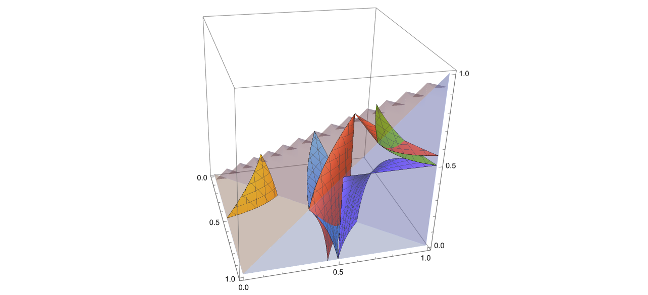
Figure 7: For $n=3$, contour $f(2)=4/9$ (red colour) comprised of two branches meeting at $p_{1}=p_{2}=p_{2}=2/3$ and crossing both ${\cal F}_{2,3}$ and ${\cal F}_{3,3}$, and contour $f(2)=1/2$ inside ${\boldsymbol{[}}{\cal F}_{2,3},{\cal F}_{3,3}{\boldsymbol{]}}$.

Proposition 3

If a closed family $\cal P$ for every $k\geq 0$ satisfies

$$\max\{h(\lambda,\boldsymbol{p}):(\lambda,\boldsymbol{p})\in{{\cal P}\cap{\boldsymbol{[}}{\cal F}_{k},{\cal F}_{k+1}{\boldsymbol{]}}}\}\geq\frac{1}{2}$$

then the family is cross modal.

Proof. The inequality $f(k;\lambda,p)\geq 1/2$ implies that $k$ is a mode, and that the likelihood maximum is attained in ${\cal P}\cap{\boldsymbol{[}}{\cal F}_{k},{\cal F}_{k+1}{\boldsymbol{]}}$. $\Box$

We take advantage of the natural order structure on $\nabla$ to introduce a reasonably large class of unperforated families ${\cal P}\subset\nabla$. Define ${\cal P}$ to be directed if $(0,{\boldsymbol{0}})\in{\cal P}$ and the following conditions hold for $k\geq 0$:

• for $(\lambda,\boldsymbol{p})\in{\cal P}$ with $m_{+}(\lambda,\boldsymbol{p})=k$ there exists $(\lambda^{\prime},\boldsymbol{p}^{\prime})\in{\cal P}$ such that

  $$(\lambda^{\prime},\boldsymbol{p}^{\prime})\geq(\lambda,\boldsymbol{p}),~{}m_{+}(\lambda^{\prime},\boldsymbol{p}^{\prime})=k+1~{}~{}{\rm and~{}~{}}f(k+1;\lambda^{\prime},\boldsymbol{p}^{\prime})>f(k+1;\lambda,\boldsymbol{p}),$$

• for $(\lambda,\boldsymbol{p})\in{\cal P}$ with $m_{-}(\lambda,\boldsymbol{p})=k+1$ there exists $(\lambda^{\prime},\boldsymbol{p}^{\prime})\in\cap{\cal P}$ such that

  $$(\lambda,\boldsymbol{p})\geq(\lambda^{\prime},\boldsymbol{p}^{\prime}),~{}m_{-}(\lambda^{\prime},\boldsymbol{p}^{\prime})=k~{}~{}{\rm and~{}~{}}f(k;\lambda,\boldsymbol{p})<f(k;\lambda^{\prime},\boldsymbol{p}^{\prime}).$$

Condition $(0,{\boldsymbol{0}})\in{\cal P}$ can always be fulfilled by including zero in the family if needed. The rationale behind the concept of directed family relates to the next property.

Lemma 2

If $(\lambda^{\prime},\boldsymbol{p}^{\prime})\geq(\lambda,\boldsymbol{p})$ for two distinct elements of $\nabla$, then $k>m_{+}(\lambda^{\prime},\boldsymbol{p}^{\prime})$ implies $f(k;\lambda^{\prime},\boldsymbol{p}^{\prime})>f(k;\lambda,\boldsymbol{p})$ provided $\lambda^{\prime}+p_{k}^{\prime}>0$.

Proof. The last condition is needed to ensure $f(k;\lambda^{\prime},\boldsymbol{p}^{\prime})>0$. We may pass from $(\lambda,\boldsymbol{p})$ to $(\lambda^{\prime},\boldsymbol{p}^{\prime})$ by successively increasing one of the components. In the course of such possibly infinitely many transitions the leading mode of intermediate vectors stays less than $k$, therefore Lemma 1 (iii), (iv) ensures that the likelihood function $f(k;\cdot)$ strictly increases on some steps, whence eventually $f(k;\lambda^{\prime},\boldsymbol{p}^{\prime})>f(k;\lambda,\boldsymbol{p})$. $\Box$

Theorem 3

Every closed directed family ${\cal P}\subset\nabla$ is cross modal.

Proof. Condition $(0,{\boldsymbol{0}})\in{\cal P}$ provides the base for induction to show that directed $\cal P$ is unperforated in a strong sense, meaning that every possible value of $m_{+}$ and $m_{-}$ is taken. Trivially $f(0;0,{\boldsymbol{0}})=1$ is the absolute maximum of $f(0;\cdot)$.

For $k>\ell\geq 0$ let $(\lambda,\boldsymbol{p})\in{\cal P}$ have $m_{+}(\lambda,\boldsymbol{p})=\ell$. By induction and the assumption there exists a increasing chain in $\cal P$ of distinct elements

$$(\lambda,\boldsymbol{p})\leq\ldots\leq(\lambda^{\prime},\boldsymbol{p}^{\prime})\leq(\lambda^{\prime\prime},\boldsymbol{p}^{\prime\prime}),$$

where the last two terms are chosen so that $m_{+}(\lambda^{\prime},\boldsymbol{p}^{\prime})=k-1,m_{+}(\lambda^{\prime\prime},\boldsymbol{p}^{\prime\prime})=k$ and $f(k;\lambda^{\prime},\boldsymbol{p}^{\prime})<f(k;\lambda^{\prime\prime},\boldsymbol{p}^{\prime\prime})$. The likelihood function $f(k;\cdot)$ is increasing strictly along the chain, as the increase holds within the last two terms by the construction and for the remaining part of the chain by Lemma 2.

For $\ell>k$ a similar chain along which the likelihood decreases is constructed backwards from $(\lambda,\boldsymbol{p})\in{\cal P}\cap{\boldsymbol{[}}{\cal F}_{\ell},{\cal F}_{\ell+1}{\boldsymbol{]}}$. It follows that the absolute maximum of $f(k;\cdot)$ can only be found in ${{\cal P}\cap{\boldsymbol{[}}{\cal F}_{k},{\cal F}_{k+1}{\boldsymbol{]}}}\}$ and it exists since $\cal P$ is closed. $\Box$

6.1 Sequences

The work of previous authors [6, 8, 21, 22, 28] observed the cross-modality of the Bernoulli sums $S_{n}=B_{1}+\ldots+B_{n}$ for $B_{1},B_{2},\ldots$ with given success probabilities, where $n$ was treated as a parameter. Bonferroni [3] was apparently the first to provide extended analysis of the peak height for the Bernoulli sums.

To embed this class of distributions in the general framework, one may consider a sequence ${\cal P}=\{(0,{\boldsymbol{0}}),(\lambda_{1},\boldsymbol{p}_{1}),(\lambda_{2},\boldsymbol{p}_{2}),\ldots\}\subset\nabla$ such that $(\lambda_{n+1},\boldsymbol{p}_{n+1})$ is derived from its predecessor $(\lambda_{n},\boldsymbol{p}_{n})$ by one of the following operations:

• replacing one of the success probabilities $p_{i}$ by a larger value $p_{i}^{\prime}>p_{i}$,

• extending the vector by including a new component $p^{\prime}$,

• incrementing the Poisson parameter by a quantity not exceeding $\gamma^{*}(\lambda_{n},\boldsymbol{p}_{n})$,

where the parameters of extension $i,p_{i}^{\prime}$ or $p^{\prime}$ may depend on $n$. Obviously, (o1), (o3) correspond to convolution with a Bernoulli or Poisson variable, respectively. The operation (o2) is a special case of (o1) ‘replacing zero by a Bernoulli variable’. The constraint in (o3) is needed to avoid decreasing likelihood. The increments of the mean satisfy $\mu(\lambda,\boldsymbol{p}_{n+1})-\mu(\lambda,\boldsymbol{p}_{n})\leq 1$, whence by Theorem 2 ${\cal P}$ is unperforated. Applying Lemma 1 (iii) we see that ${\cal P}$ is directed, hence cross modal. If $\mu(\lambda,\boldsymbol{p}_{n})\to\infty$ as $n\to\infty$, the family has infinite range.

A well-known example is the Karamata-Stirling distribution, which we record with two parameters

$$f(k;n,t)=\left[{n\atop k}\right]\frac{t^{k}}{(t)_{n}},~{}~{}~{}t>0,~{}1\leq k\leq n.$$ (21)

This is a Poisson-binomial distribution with the success probabilities $p_{i}=t/(t+i-1),i\geq 1$ (note: $p_{1}=1$). The $t=1$ case relates to the random records model, and the general $t>0$ case plays a major role in the study of permutations, partitions and other combinatorial structures [1]. With the aid of asymptotic expansion of the distribution, Kabluchko et al [14] have found approximation for the peak height and showed that for large enough $n$ the mode is unique and coincides with $\lfloor u(n,t)-1/2\rfloor$ or $\lceil u(n,t)-1/2\rceil\}$, where $u(n,t):=t\,(\log n+\partial_{t}\log\Gamma(t)),$ with the exact formula $m_{\pm}(n,t)=\lfloor u(n,t)\rfloor$ being valid for a set of $n$’s of asymptotic density $1$ (though not for all $n$). As has been noticed in [23], Darroch’s rule applied to this instance gives bounds for all $n$

$$\lfloor\mu(n,t)\rfloor\leq m_{\pm}(n,t)\leq\lceil\mu(n,t)\rceil~{}~{}~{}{\rm for}~{}~{}\mu(n,t)=\sum_{i=1}^{n}\frac{t}{t+i-1},$$

and essentially reduces the localisation to the asymptotic expansion of the shifted harmonic numbers, for which we refer to $\mu(n,t)/t$ [10]. The uniqueness of the mode in case of irrational $t$ is also immediate. A new twist we wish to add is that the maxima of (21) in $n$ are those values where the mode increases, that is the likelihood maximiser is the inverse function to the mode, like in the binomial scheme in Figure 2. We leave for now the interpretation through waiting times open.

There are many examples of row-wise totally positive triangular arrays of combinatorial numbers [23, 24], leading to Bernoulli sums with parameters $\boldsymbol{p}_{n}$ not explicitly known and not following the simple patterns (o1) or (o2). Stochastic monotonicity of the associated sums $S_{n}$ is a necessary but not sufficient condition for Theorem 3 to work. A numerical evidence suggests that the array of normalised Stirling numbers of the second kind is cross modal. See Rukhin et al [25] for a related study of the likelihood ratios for a convolution of two binomial distributions.

6.2 Power series and other continuous-parameter families

For $a_{0}>0,r_{i}>0$ with $\sum_{i}r_{i}<\infty$ consider the entire function of the form

$$F(t)=\sum_{k=0}^{\infty}a_{k}t^{k}=a_{0}e^{\lambda t}\prod_{i=1}^{\infty}(1+r_{i}t),$$ (22)

which defines a power series family of logconcave distributions with parameter $t\geq 0$.

The distribution with parameter $t=1$ is the law of an extended Bernoulli sum $S(\lambda,\boldsymbol{p})$ with Poisson parameter $\lambda$ and success probabilities $p_{i}=r_{i}/(1+r_{i})$, as in (14). For the generic $t\geq 0$ the distribution has probability generating function

$$\frac{F(tz)}{F(t)}=\frac{a_{0}}{F(t)}e^{\lambda tz}\prod_{i=1}^{\infty}(1+r_{i}tz),$$

corresponding to the extended Bernoulli sum with Poisson parameter $t\lambda$ and odds $tr_{i}$. This family of power series distributions is cross modal by Proposition 2 which in turn followed from the extended Darroch’s rule in Theorem 2. The theorem also implies that the criterion in Proposition 1holds with strict inequalities $t_{k}<\ell(k)<t_{k+1}$ and $k-1<\mu(t_{k})<k$ (last for $k\geq 1$) Compare with $\mu(t_{k})=k$ in the pure Poisson case.

Taking a geometric view will lead to a surprising conclusion, essentially matching the initial intuition that ‘the mean and the mode grow at about the same pace’ was correct. Note that in the parametrisation by odds the power series family corresponds to a ray. In terms of the success probabilities the family has parameters $(\lambda(t),\boldsymbol{p}(t))$, where

$$\lambda(t)=\lambda t,~{}~{}{\rm and}~{}~{}p_{i}(t)=\frac{tp_{i}}{1-p_{i}+tp_{i}}$$ (23)

are increasing functions. Geometrically, $(\lambda(t),\boldsymbol{p}(t)),t\geq 0,$ is a continuous curve in $\nabla$, which is increasing (in the partial order) and unperforated since $\mu(\lambda(t),\boldsymbol{p}(t))\uparrow\infty$. The family is directed. Indeed, interpret $t_{k}$ and $t_{k+1}$ as the ‘time’ when the curve enters into, respectively, exits from ${\boldsymbol{[}}{\cal F}_{k},{\cal F}_{k+1}{\boldsymbol{]}}$. Lemma 2 tells us that $f(k;\lambda(t),\boldsymbol{p}(t))$ strictly increases for $t\leq t_{k}$ and strictly decreases for $t\geq t_{k+1}$ thus the likelihood attains its absolute maximum inside ${\boldsymbol{[}}{\cal F}_{\ell},{\cal F}_{\ell+1}{\boldsymbol{]}}$. Moreover by Lemma 1 (iii), we have $\partial_{t}f(k;\lambda(t_{k}),\boldsymbol{p}(t_{k}))>0$ and $\partial_{t}f(k;\lambda(t_{k+1}),\boldsymbol{p}(t_{k+1}))<0$, understood as transversal crossing the contours of the likelihood function. It again follows that the family of extended Bernloulli sums defined by the totally positive power series (22) is cross modal. But neither general criterion for logconcave families in Proposition 1 (iii) nor the proof of Theorem 3 rely on the Darroch’s rule, therefore the rule becomes a consequence. So to summarise: since every extended Bernoulli sum is a member of a power series family (23), the cross modality of the family implies the extended Darroch’s rule. Scrutinising this way of reason, three ingredients have been used: matching the mean by the likelihood maximisation for power series families, including distribution in such a family and the elemenrary recursion in Lemma 1 (i) observed long ago by the pioneers [3, 7].

The roots of some totally positive entire functions (22) are known explicitly. For the example in Figure 4 the Weierstrass product formula applied to $\cosh{\sqrt{t}}$ gives the parameters of extended Bernoulli sum as $\lambda=0$ and

$$p_{i}=\frac{4}{4+(1-2i)^{2}\pi^{2}},~{}~{}i\geq 1.$$

Karamata-Stirling family of distributions (21) relates to a totally positive polynomial, for which we conclude on the cross modality now in the variable $t$.

7 Breaking the mode

The value of Darroch’s rule for localising the mode lies in the simplicity of the mean as compared to the whole multiparameter profile $(\lambda,\boldsymbol{p})$, which may not be known explicitly. Bur even with $(\lambda,\boldsymbol{p})$ given, it looks hard to control the mode under the (o2)-deformations of the profile. From Theorem 1 we only infer that increasing a particular $p_{i}$ will break the mode if the success probability is smaller than a certain bound depending on $(\lambda,\boldsymbol{p})$.

The peak skewness is an alternative characteristic of stability of the mode. Recall that $\gamma^{*}(\lambda,\boldsymbol{p})$ is the minimal parameter of Bernoulli variable needed to transport the mode to larger position. The monotonicity properties of $\gamma^{*}(\lambda,\boldsymbol{p})$ agree with its interpretation as a size of effort to break the mode, that is

$$\partial_{p_{i}}\gamma^{*}(\lambda,\boldsymbol{p})<0,~{}~{}~{}\partial_{\lambda}\gamma^{*}(\lambda,\boldsymbol{p})<0$$

in consequence of monotonicity of the likelihood ratio and the formula

$$\gamma^{*}(\lambda,\boldsymbol{p})=\left(1+\frac{1-\frac{f(m-1)}{f(m)}}{1-\frac{f(m+1)}{f(m)}}\right)^{-1},$$

where for shorthand $m=m_{+}(\lambda,\boldsymbol{p})$. Curiosly, there is some connection with the mean. In particular, if $(\lambda,\boldsymbol{p})\in{\cal M}_{k}$ one needs to increase the mean by at least $1/(k+2)$ to increment the leading mode by one, hence $\gamma^{*}(\lambda,\boldsymbol{p})\geq 1/(k+2)$. On the other hand, if $(\lambda,\boldsymbol{p})\in{\cal F}_{k}$ (the twin mode case), to increment the leading mode the mean should be increased by at least $1-1/(k+1)$ while $\gamma^{*}(\lambda,\boldsymbol{p})=1$.

7.1 Two Bernoulli increments versus one

The above begs a question: how to transport the mode of $S$ by adding independent Bernoulli or Poisson variables in the most economic way, as measured by the mean?

To that end, suppose $S$ has probability function $f(k)$ with leading mode $m$, and we add an independent variable $Z$. A minute thought shows that shifting the mode to $m+1$ amounts to a linear programming problem with the balance equation as a constraint

$${\mathbb{P}}[S+Z=m]={\mathbb{P}}[S+Z=m+1],$$

and the objective functional ${\mathbb{E}}Z$, where $Z$ can be restricted to have the support within $\{0,1,\ldots,m+1\}$. If we only consider $Z$ with a two-point distribution ${\mathbb{P}}[Z=s]=\delta$, ${\mathbb{P}}[Z=0]=1-\delta$ with given $s$, then the minimal necessary value of $\delta$ is found from the balance equation as

$$\delta=\frac{\Delta f(m)}{\Delta f(m)-\Delta f(m-s)},$$

(generalising $\gamma^{*}(\lambda,\boldsymbol{p})$ in the $s=1$ case) which incurs the transportation cost $s\delta$. For convexity reasons, if no constraint on the distribution of $Z$ is imposed, the optimal distribution is two-point, with the range parameter found as the minimiser in

$$\min_{s}\frac{s\Delta f(m)}{\Delta f(m)-\Delta f(m-s)},$$ (24)

and $\delta=\delta(s)$ determined as above.

Within the class of extended Bernoulli sums, for the sake of optimisation it is sufficient to consider $Z$ representable as a Bernoulli sum with at most $m+1$ terms. In the case $m=0$ the optimal transport involves a Bernoulli variable $Z$ with the success probability $\gamma^{*}(\lambda,\boldsymbol{p})$. For $m>0$ we are willing to show that this one-term solution might not be optimal. Indeed, comparing $s=1$ and $s=2$ instances of (24), the second will be more less costly if

$$\frac{2\Delta f(m)}{\Delta f(m)-\Delta f(m-2)}<\frac{\Delta f(m)}{\Delta f(m)-\Delta f(m-1)},$$

which is equivalent to

$$A:=\Delta^{3}f(m-2)<0.$$ (25)

Condition (25) is necessary for a two-term Bernoulli sum with some success probabilities $\alpha_{1},\alpha_{2}$ to outperform a single Bernoulli with parameter $\gamma^{*}(\lambda,\boldsymbol{p})$. Lemma 1 (viii) entails the expansion

$$f(k;\lambda,\boldsymbol{p}\cup\alpha_{1},\alpha_{2})=f(k;\lambda,\boldsymbol{p})-(\alpha_{1}+\alpha_{2})\Delta f(k;\lambda,\boldsymbol{p})+\alpha_{1}\alpha_{2}\Delta^{2}f(k;\lambda,\boldsymbol{p}),$$ (26)

which allows us to write the balance equation

$$f(m;\lambda,\boldsymbol{p}\cup\alpha_{1},\alpha_{2})=f(m+1;\lambda,\boldsymbol{p}\cup\alpha_{1},\alpha_{2})$$

in the form

$$C+(\alpha_{1}+\alpha_{2})B+\alpha_{1}\alpha_{2}A=0,~{}~{}~{}{\rm where}~{}~{}C:=\Delta f(m),B:=-\Delta^{2}f(m-1),$$ (27)

and we have $C>0,B<0$ since $m$ is the mode. In this notation, the peak skewness becomes $\gamma^{*}(\lambda,\boldsymbol{p})=-C/B$, which substituted in the balance equation yields

$$C+(\alpha_{1}+\alpha_{2})B+\alpha_{1}\alpha_{2}C=C+\gamma^{*}(\lambda,\boldsymbol{p})B,$$

and therefore

$$\alpha_{1}+\alpha_{2}-\gamma^{*}(\lambda,\boldsymbol{p})=-\alpha_{1}\alpha_{2}\,\frac{A}{B}<0,$$

showing that two Bernoulli variables may be better than one. To find the desired parameters explicitly, set $\alpha:=\alpha_{1}=\alpha_{2}$ and solve the balance equation $C+2B\alpha+A\alpha^{2}=0$ as

$$\alpha=\frac{-B-\sqrt{B^{2}-AC}}{A}.$$

It is readily checked that $2\alpha<-C/B$ indeed holds and thus $0<\alpha<1$. In accord with [7] the optimum has been found in the class of binomial distributions.

Thus condition (25) turns also sufficient. We have found numerically examples of $S$ with $A<0$, for instance the Binomial$(12,0.385)$ distribution has $m=5$ and $A=-0.003$, which gives a tiny advantage to perturbation of $Z$ by a single term.

The form of balance equations with $Z$ being a sum of $d\geq 3$ independent Bernoulli variables can be guessed from (26) and (27). However, the case of two terms suggests that to get some further improvement $\Delta^{d}f(m-d+1)$ should disagree with the sign-alternating pattern emerging by the normal approximation.

7.2 Breaking the Poisson mode

Consider $S\stackrel{{\scriptstyle d}}{{=}}{\rm Poisson}(t),~{}~{}m<t<m+1$. Adding $Z\stackrel{{\scriptstyle d}}{{=}}$Poisson$(k+1-t)$ shifts the mode to $m+1$, but adding a Bernoulli variable with success probability

$$\gamma^{*}(t,{\boldsymbol{0}})=\frac{(m+1)t-t^{2}}{2(m+1)t-t^{2}-m(m+1)}$$

offers a more spare mode transport with $\gamma^{*}(t,\boldsymbol{p})<m+1-t$, the inequality holding since the cubic polynomial

$$((m+1)t-t^{2})-[(2(m+1)t-t^{2}-m(m+1))(m+1-t)]$$

is strictly positive in the interval $(m,m+1)$. From $\Delta^{3}f(m-2)>0$ follows that no two-term deformation transporting the mode could have smaller mean.

Acknowledgement The author is indebted to Alex Marynych, Jim Pitman and Michael Farber for inspiring discussions, help with terminology and pointers to the literature.

References

• [1] R. Arratia, A.D. Barbour and S. TavarΓ©, Logarithmic combinatorial structures, EMS, 2003.
• [2] B.M. Baker and D.E. Handelman (1992), Positive polynomials and time dependent integer-valued random variables, Can. J. Math. 44, 3–41.
• [3] C.E. Bonferroni (1933), Sulla probabilitΓ‘ massima nello Schema di Poisson, Giorn. Ist. Ital. Attuari 4, 109–115. (review in German in zbMATH Zbl 0007.02302 and JFM 59.1157.05)
• [4] R. Bott (1954), Nondegenerate critical manifolds, Ann. Math. 60, 248–261.
• [5] T. Broderick, M. Jordan and J. Pitman (2013), Feature allocations, probability functions, and paintboxes, Bayesian Analysis 8, 801–836.
• [6] F.T. Bruss and D. Paindaveine (2000) Selecting a sequence of last successes in independent trials, J. Appl. Probab. 37, 389–399.
• [7] P.L. Chebyshev (1846), DΓ©monstation Γ©lΓ©mentaire d’une proposition gΓ©nΓ©rale de la thΓ©orie des probabilitΓ©s, J. Reine und Angew. Math. 33, 259–267.
• [8] E. Cramer (2000), Asymptotic estimators of the sample size in a record model, Statistical Papers 41, 159–171.
• [9] J.N. Darroch ( 1964), On the distribution of the number of successes in independent trials, Ann. Math. Stat. 35, 1317–1321.
• [10] P. Flajolet and R. Sedgewick, Analytic combinatorics, CUP, 2009.
• [11] W. Hoeffding (1956), On the distribution of the number of successes in independent trials, Ann. Math. Statist. 27, 713–721.
• [12] S. Dharmadhikari and K. Joag-Dev, Unimodality, convexity, and applications, Academic Press, Boston, 1988.
• [13] K. Jogdeo and S.M. Samuels (1968), Monotone convergence of binomial probabilities and a generalization of Ramanujan’s equation, Ann. Math. Statist. 39, 1191–1195.
• [14] Z. Kabluchko, A. Marynych and H. Sulzbach (2016), Mode and Edgeworth expansion for the Ewens distribution and the Stirling numbers, J. Integer Seq. 19, No. 8, Article 16.8.8.
• [15] S. Karlin, Total positivity Vol I, Stanford University Press, 1968.
• [16] J. Keilson and H. Gerber (1971), Some results on discrete unimodality, J. Amer. Statist. Assoc. 66, 86–89.
• [17] P. LΓ©vy, ThΓ©orie de l’addition des variables alΓ©atoires, Gauthier-Villars, Paris, 1937.
• [18] Liggett, T. M. (1997). Ultra logconcave sequences and negative dependence. J. Combin. Theory Ser. A 79, 315–325.
• [19] M. Madimana, J. Melbourne and C. Roberto (2023), Bernoulli sums and RΓ©nyi entropy inequalities, Bernoulli 29, 1578–1599.
• [20] A.W. Marshall, I. Olkin and B.C. Arnold, Inequalities: Theory of majorization and its applications (2nd edition), Springer, 2011.
• [21] J.L. Moreno-Rebollo, I.L. Barranco-Chamorro, F.G. LΓ³pez-BlΓ‘zquez, T. GΓ³mez-GΓ³mez (1996), On the estimation of the unknown sample size from the number of records. Statist. Probab. Lett. 31, 7–12.
• [22] J.L. Moreno-Rebollo , F.Lopez-Blazquez, I. Barranco-Chamorro and A. Pascual-Acosta (2000), Estimating the unknown sample size, Journal of Statistical Planning and Inference 83, 311–318.
• [23] J. Pitman (1997), Probabilistic bounds on the coefficients of polynomials with only real zeros, J. Combin. Theory, Ser. A 77, 279–303.
• [24] D. Pollard, Probability tools, tricks, and miracles, Chapter 4 of the book draft, http://www.stat.yale.edu/~pollard/
• [25] A. Rukhin, C. E. Priebe and D.M. Healy Jr. (2009), On the monotone likelihood ratio property for the convolution of independent binomial random variables, Discrete Applied Mathematics 157, 2562–2564.
• [26] S.M. Samuels (1965), On the number of successes in independent trials, Ann. Math. Statist. 36, 1272–1278.
• [27] A. Saumard and J. A. Wellner (2014), Log-concavity and strong log-concavity: A review, Statistics Surveys 8, 45–114.
• [28] M. Tamaki (2010), Sum the multiplicative odds to one and stop, J. Appl. Prob. 47, 761–777.
• [29] W. Tang and F. Tang (2023), The Poisson Binomial Distributionβ€” Old& New, Statist. Sci. 38, (1) 108–119.
• [30] J. Wellner (2013), Strong log-concavity is preserved by convolution, Progress in Probability 66, 95–102.