remarkRemark \newsiamthmclaimClaim \newsiamremarkexampleExample \headersSurface elevation errors in Stokes modelsE. Bueler
Surface elevation errors in finite element
Stokes models for glacier evolution
Abstract
The primary data which determine the evolution of glaciation are the bedrock elevation and the surface mass balance. From this data, which we assume is defined over a fixed land region, the glacier’s geometry solves a free-boundary problem which balances the surface velocity from the Stokes flow with the surface mass balance. A surface elevation function for this problem is admissible if it is above the bedrock topography, equivalently if the ice thickness is nonnegative. For an implicit time step, this free-boundary problem can be posed in weak form as a variational inequality. After some preparatory theory for the glaciological Stokes problem, we conjecture that the continuous-space, implicit time step problem for the surface elevation is well-posed. This conjecture is supported both by physical arguments and numerical evidence. We then prove a general theorem which bounds the error made by a finite element approximation of a nonlinear variational inequality in a Banach space. The bound is a sum of error terms of different types which are special to variational inequalities. In the case of the implicit-step glacier problem these terms are of three types: errors from discretizing the bed elevation, errors from numerically solving for the Stokes velocity, and finally an expected quasi-optimal finite element error in the surface elevation itself.
keywords:
error bounds, finite element methods, glaciers, ice flow, variational inequalities1 Introduction
Glacier and ice sheet simulations model the ice as a free-surface layer of very-viscous, incompressible, and non-Newtonian fluid [22, 40]. For simplicity we will only consider simulations of land-based glaciers, without floating portions, and we note that an “ice sheet” is simply a continent-scale glacier.
The two essential input data into such simulations are the bedrock elevation, which is assumed here to be independent of time, and the time-dependent surface mass balance rate (SMB; the climatic mass balance rate [13]). By definition, the SMB is the balance between accumulating snow and the loss of melt water, through runoff, at the upper surface of the glacier [13]. Note that elevations are measured here in meters, and SMB is measured in ice-equivalent units of meters per second.
Thus a glacier simulation takes, as inputs, the bedrock topography, a (generally) time-dependent climate, and an initial geometry. The simulation produces the glacier’s evolving geometry and flow velocity; these are the output fields of primary scientific value. Additional complications are common in comprehensive models [40, 41]. For example, the internal energy [3] or temperature of the ice may be tracked, and/or there may be models of liquid water within the ice matrix or at ice surfaces. However, for simplicity and concreteness we only consider conservation of mass and momentum, but not of energy, and liquid water will play no role. Furthermore we will assume zero velocity, i.e. a non-sliding and non-penetrating condition, at the base of the ice. On the other hand, we will not make the shallowness assumptions which are common in comprehensive ice sheet models.
One may parameterize the glacier’s geometry using either the (upper) surface elevation or the ice thickness. At a time and map-plane location where a glacier exists the surface elevation must exceed the bedrock elevation, equivalently the ice thickness must be positive. The computed flow velocity is only defined at those locations and times where ice is present, namely on an evolving 3D domain between the bedrock and surface elevations. In other words, the surface elevation and thickness functions must satisfy inequalities to be admissible.
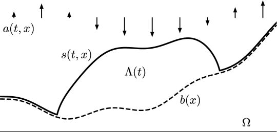
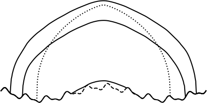
Our notation is sketched in Figure 1. Let be a fixed portion of land, with map-plane coordinates . All time-dependent quantities are assumed to be defined on for some . On assume that we are given, as data, a real and continuous bed elevation function , and a real, signed, and continuous SMB function . In areas of where (accumulation; downward arrows in Figure 1), a glacier will exist. If (upward arrows) then either a glacier exists with an ablating surface, because of flow from accumulation areas, or no glacier exists. Determining which situation applies at given coordinates requires solving free-boundary problems like those considered in this paper.
Let be the (solution) ice surface elevation. We will regard this as defined for all , but subject to the constraint that the surface must be at or above the bedrock (). In regions with no ice holds. The solution ice velocity and pressure are then defined only on the open 3D domain
| (1) |
This aspect of glacier modeling deserves emphasis: The time-dependent 3D domain , on which the velocity and pressure are meaningful, is determined by the evolving surface elevation , which is itself part of the model solution.
The surface trace of the ice velocity will be of importance; it is reconsidered in a precise Sobolev space context in Section 2. We extend it by zero so that it is defined everywhere in :
| (2) |
Compare flux extension by zero in [40]. Also let denote an un-normalized and upward surface normal vector. (This is assumed well-defined for current purposes, but compare Section 3.) An infinite-dimensional nonlinear complementarity problem (NCP) [6, 17, 40] applies almost everywhere in :
| (3a) | ||||
| (3b) | ||||
| (3c) | ||||
System (3) says that either a location is ice free (), where the climate is locally ablating (), or that the surface kinematical equation (SKE) holds:
| (4) |
This equation says that the (non-material) surface of the ice moves vertically according to the sum of the SMB and a component of the ice velocity at the surface [40]. Equation (4) is a statement of mass conservation at the surface [3], sometimes called the free-surface equation [33] or the kinematic boundary condition111Note that equation (4) is not a boundary condition of any identifiable PDE problem. [22].
We believe that glaciologists agree with the conditions of NCP (3) as a model for glaciers. For example, in numerical ice sheet models the SKE (4) is a standard way for surface geometry to evolve [22, 40]. The idea that positive (continuous) SMB at a given location implies the existence of glacier ice there is not controversial. Equivalently, ice-free conditions are understood to exist only where the SMB is negative, because any accumulation (positive SMB) would immediately become glacier ice (by definition).
In the current paper the SMB is necessarily assumed to be defined everywhere in , regardless of whether a glacier is present or not. This is because a simulated glacier needs to be able to advance into unglaciated locations. In ice-free areas the SMB should have the value which a glacier surface would experience at that time and location. Thus the value can be modeled using precipitation and an energy balance [22], for instance by hypothesizing an ice surface and then computing the balance of snow accumulation minus ablation (using the energy available for melt).
The non-shallow ice dynamics model considered in this paper, which conserves mass and momentum, is the non-sliding (e.g. frozen) base, isothermal, shear-thinning (non-Newtonian), and incompressible Stokes problem [22, 28, 40]. This model is applied over the domain defined in (1) above. Let be the upper surface and be the base . The possibility of cliffs at the ice margin is neglected, so is assumed to hold at any time. To state the shear-thinning (Glen’s) flow law, let denote the strain rate tensor, with Frobenius norm (summation convention). The effective ice (dynamic) viscosity [22] is then given by a regularized formula
| (5) |
The exponent , often written , is approximately 4/3 in practice [22]. The coefficient has p-dependent units, while has SI units . The values of n and can be determined from measured properties of ice [21, 22], including temperature, but both are assumed to be constant here. Note that yields a Newtonian fluid with constant viscosity, while for the regularization implies that is bounded above. Assume that the density of ice and the acceleration of gravity are constant. At each time the modeled glacier has velocity and pressure solving the following 3D fluid equations:
| (6a) | within | ||||
| (6b) | ” | ||||
| (6c) | on | ||||
| (6d) | on | ||||
Boundary condition (6c) says that the sub-aerial upper surface is stress free; this must not be confused with the SKE (4).
In summary at this point, we assume that a glacier simulation is an evolving free-surface flow, subject to a signed climate that can add or remove ice, coupled to a nonlinear Stokes problem which must be solved within an evolving, 3D icy domain. The initial/boundary value problem consisting of (1)–(6) requires data plus an initial surface elevation . The solution variables are , , and , with defined everywhere over , but subject to , and with defined on for each (equation (1)). The surface elevation and surface velocity trace are linked by the kinematical NCP (3).
Note that the NCP (3) is the only place where a time derivative appears in the model statement; the SKE (4) is a consequence of this NCP. Because the flow is very viscous [1], the Stokes sub-model (5)–(6) acts as an instantaneous “algebraic” constraint on the evolution statement in (3). The coupled, infinite-dimensional problem of determining the evolving geometry of a glacier, namely system (1)–(6), is therefore simultaneously a differential algebraic equation system [2, 33] and an NCP.
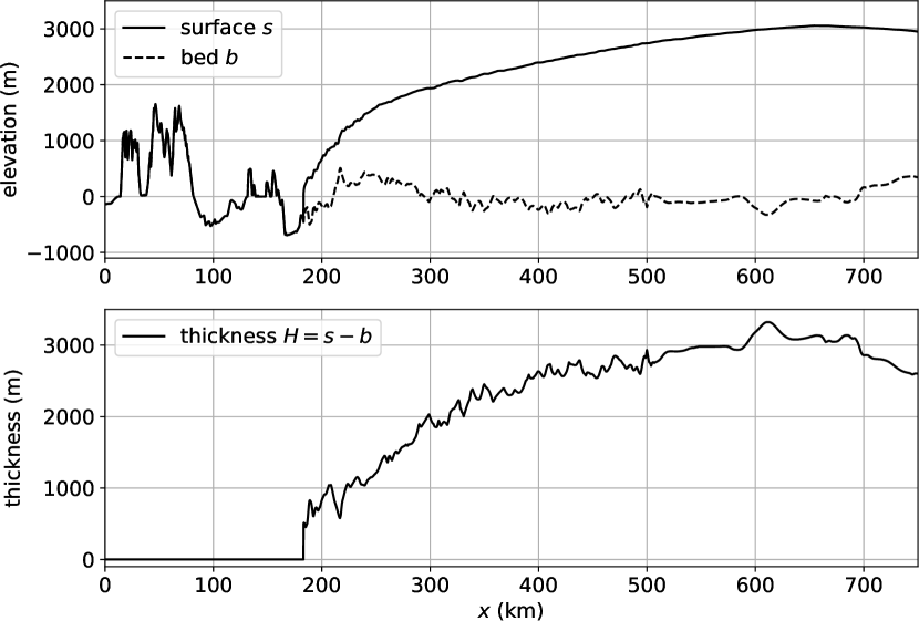
While essentially equivalent in the continuum problem, formulations using thickness functions to parameterize geometry have different character from those using surface elevation, as here, when the bedrock is realistically rough. Surface elevation will be preferred because of the flow-caused smoothing effect illustrated in Figure 2. That is, we observe that for land-based glaciers is smoother in than the thickness because the latter “inherits” the lower regularity of the (typically) eroded and faulted bedrock topography .
Glacier simulations are commonly formulated using a finite element (FE) method for the Stokes sub-problem [25, 27, 36], or for a shallow approximation thereof. However, to the author’s knowledge all existing non-shallow (Stokes) evolution models use a explicit time-stepping scheme for the geometry, for example as in [27] or [33], with the one exception of the exploratory model in reference [42].
This work considers implicit time steps for the theoretical reasons addressed in Section 4. For a time step , the solution , from applying the backward Euler scheme to NCP (3), satisfies the conditions of a similar NCP:
| (7a) | ||||
| (7b) | ||||
| (7c) | ||||
For clarity we have collected-together a source term , which is assumed known. The essential approach of this paper starts in Section 3, where we re-write NCP (7) as a weak form variational inequality (VI) problem. Based on conjectured well-posedness for that problem (Section 4), our main results are in Sections 6 and 7. We prove new estimates on the numerical error which arises from solving the surface elevation VI problem by FE approximation.
Observe that the backward Euler scheme chosen for problem (7) is merely the simplest A-stable scheme which can be applied to the continuous time problem (3). Extension to higher-order A-stable and/or stiff decay [2] schemes is obviously of interest, but we do not pursue them because the problem (7) already contains all the important features. For finite-dimensional differential algebraic equation problems, such implicit schemes are the standard choices [2], given the stiffness exhibited by such systems. In the infinite-dimensional case here, where the SKE (4) is constrained at any time by the “algebraic” Stokes problem (5)–(6), implicit schemes are in fact the natural choice.
One can also make a case for implicit time-stepping based on simulation performance, that is, by comparing to the conditionally-stable explicit alternatives [7]. However, this assumes that NCP (7) can be solved efficiently, and that the implicit scheme turns out to have unconditional stability. In fact, neither efficiency nor stability are addressed in the current paper.
This paper is organized as follows. Section 2 recalls the theory of the Glen-law Stokes problem on a fixed domain, and we add an apparently-new bound on the surface trace of the velocity solution (Corollary 2.8). In Section 3 we reformulate the coupled NCP problem (5)–(7) as a VI weak form. The key coupling term is the surface motion term in SKE (4), for which we provide a quantitative bound over a Sobolev space of surface elevation functions (Lemma 3.4). However, this bound is subject to Conjecture 3.3, which hypothesizes that the surface velocity trace is Lipschitz continuous with respect to surface elevation. Well-posedness for each implicit step VI problem is considered in Section 4, based upon Conjecture 4.1 hypothesizing the coercivity of the same surface motion term. Certain physical and modeling ideas are discussed in Section 4, as context needed to understand Conjecture 4.1, followed in Section 5 by some numerical evidence for the validity of this Conjecture. At this point we have in hand a mathematically-precise time-discretized model, though with only conjectural well-posedness (Theorem 4.2). This continuum model is apparently stated here for the first time. Turning to FE approximations, in Section 6 we prove an abstract FE error estimate, Theorem 6.3 and its Corollaries, for general VI problems involving nonlinear operators on Banach spaces. This new estimate, which makes coercivity and Lipshitz assumptions on the operator, extends the classical bilinear case by Falk [18]. In Section 7 we apply the abstract estimate to the glacier problem, yielding our final result which is Theorem 7.2. The physical significance of each term in this error estimate, and how associated FE method choices are made, is addressed at the end.
We will use only these few abbreviations: FE (finite element), NCP (nonlinear complementarity problem), PDE (partial differential equation), SIA (shallow ice approximation), SKE (surface kinematical equation), SMB (surface mass balance), and VI (variational inequality).
2 The surface velocity from a glacier Stokes problem
In this Section we consider the weak form of the non-sliding, isothermal, and Glen-law Stokes sub-model (5)–(6). This sub-model, which is applied on a 3D domain , defined by (1) at a particular time , computes the surface velocity field which appears in NCP (3). We will return to that the larger model in Section 3.
We assume that the ice base , on which a Dirichlet condition holds, has positive measure, and that the remaining Neumann boundary is sufficiently-smooth so that a zero normal stress condition can be applied.
Suitable function spaces for Stokes problem (5)–(6) are then well-known. Let . Denote the Sobolev space [16] of real-valued functions with pth-power integrable first derivatives by , and let
| (8) |
be the corresponding space of vector-valued functions with trace zero along . Let be a representative vertical glacier dimension. We define the norm on by
| (9) |
Here is the 3D volume element, which will generally be suppressed in integrals. Note that denotes the Euclidean norm, while is the Frobenius norm of . Remark 1.2.1 in [5] explains the length scaling in (9), such that has consistent units.
Let where is the conjugate exponent. Define
| (10) |
as the mixed space of admissible velocity and pressure pairs. For define
| (11) |
where (summation convention). The (mixed) weak form of the Stokes sub-model seeks the solution satisfying
| (12) |
Jouvet and Rappaz [28] have proven that problem (12) is well-posed if the Neumann portion of is . Their proof uses the equivalence of (12) and the minimization of a convex and coercive functional over the divergence-free subspace . Our regularization in Glen law (5) differs from that in [28], but the necessary modifications are addressed in [25]. Note that if the weak solution is sufficiently regular then the strong form (6) is also satisfied.
Our primary purpose, resumed in the next Section, is to study the glacier geometry NCP (3), and its weak form. For that analysis we now bound the surface trace in terms of certain geometric properties of . This uses several inequalities.
Lemma 2.2 (Poincaré’s inequality; (7.44) in [19]).
Lemma 2.3 (Korn’s inequality; to prove set to the identity in Corollary 4.1 of [38]).
Under the same assumptions, there exists a dimensionless constant so that
| (14) |
The main idea of the following a priori bound is that velocity solution is controlled by geometric properties of the domain , including the constants in the above inequalities, along with certain physical constants. We will denote the ice volume by .
Lemma 2.4.
Suppose is the solution from Theorem 2.1. Then there is depending on p, , , , , , , and so that
| (15) |
Proof 2.5.
From (12) and it follows that
| (16) |
Apply Korn’s inequality, the facts that and , and equation (5):
| (17) | ||||
By equation (16) and Hölder’s inequality we thus have
| (18) | ||||
By Lemma 2.2,
| (19) |
Let . We have proved that
| (20) |
for and some constants . Note that is smooth with and as , so there exists a right-most root with . Since we have . This proves (15) with .
Lemma 2.6 (Trace inequality).
Under the assumptions of Theorem 2.1, there exists a dimensionless constant so that for all ,
| (21) |
where on the left is the trace on , and denotes the area element over .
Proof 2.7.
Theorem 5.5.1 in [16] defines a trace operator , and a constant , dependent only on p and , so that
| (22) |
for . However, because along , . The result follows if we define .
3 The weak-form implicit time-step model
Now we return to the implicit time-stepping scheme for updating the surface elevation in a model based on Stokes dynamics, namely NCP (7). Recall how this problem is derived. Let be any increasing sequence of times in , with . Let denote the generic step length. Let be the (temporal) average of the data over . Suppose that approximates the surface elevation at time . Using a backward Euler implicit step [2], SKE (4) becomes
| (24) |
(The unknown appears both in the surface velocity and slope .) For cleaner appearance, clear the denominator in (24) and define
| (25) |
However, as noted in the Introduction, in (24) actually solves a problem of free-boundary type, which is NCP (7). In particular, complementarity equation (7c) says that, at the solution time and almost everywhere over , either there is no ice () or equation (24) holds. Of course, does not solve (24) over the bare ground part of where .
The strong form NCP (7) has a weak-form variational inequality (VI; [16, 30]) version which is better-suited to both well-posedness theory and finite element (FE) analysis. Let us regard the precise Banach space of surface elevations as unknown (for now). The admissible surface elevations come from a convex and closed subset
| (26) |
(The fixed (Dirichlet) boundary condition is included into the definition of .) The VI is then derived as follows via the argument from [6]. Suppose that is a sufficiently-regular solution of NCP (7). Let be the (measurable) subset of on which constraint (7a) is inactive, where glacier ice is present: . From (7c), integration over shows that
| (27) |
for any . On the other hand, suppose is the active (ice-free) region for constraint (7a). Observe that (7b) says that on .222Note the role of extension by zero (2) here. Note that on if . Therefore integration yields an inequality:
| (28) |
Almost everywhere, either land is glacier covered (within ) or ice-free (), so addition of (27) and (28) gives the following VI for :
| (29) |
This integral inequality is known to be true of in advance of knowledge about the ice-covered part of .
Now, well-posedness of the weak-form Stokes problem (12) over a 3D domain , plus the surface trace bound in Corollary 2.8, allows us to create a well-defined map from an admissible surface elevation to the corresponding surface velocity solution . The map is defined via definition (1) of , followed by the solution of (12) over , evaluation of the trace of along (Corollary 2.8), and then definition (2) (which includes extension by zero). For this map to be well-defined, must be admissible () and sufficiently regular so that these steps are justified. We call
| (30) |
the surface motion map. It maps the scalar surface elevation to the dynamical term in the SKE (24). Constructing a bound for will help to identify a Banach space in which to seek admissible solutions .
As before, let be a bounded domain. Let be a representative horizontal scale; compare (9). For any and we define
| (31) |
Lemma 3.1 (Preliminary bound on ).
Proof 3.2.
Observe that is the surface area element for . Let be the conjugate exponent to . Apply the triangle inequality, and Hölder’s inequality twice:
| (33) | ||||
If is the a priori bound from (23) then
| (34) |
Note that if then , so
| (35) | ||||
Since , by Sobolev’s inequality333For example, apply Theorem 8.8 from [32] using , , , and . we also have , which yields (32).
The key assumption in Lemma 3.1 is that implies that the domain is nice enough so that Corollary 2.8 gives a finite bound. The key conclusion is that , the dual space. This conclusion will be critical in analyzing the weak form of NCP (7).
Now we conjecture that for some444The reason for requiring will be seen in Lemma 3.4. It would seem to be a technical requirement, as Section 7 demonstrates well-behaved numerical results using the more convenient exponent . , the -norm of the surface trace is Lipschitz as a function of . Note that we do not assume that is continuous, only that it is a measurable function defined over all of .
Conjecture 3.3.
There exists with the following two properties: (i) If is admissible ( and on ) then the conclusion of Theorem 2.1 applies, giving a well-defined surface velocity . (ii) If also is admissible, yielding different values , then there exists , independent of and , such that
| (36) |
From now on we will assume Conjecture 3.3 holds for some . We define
| (37) |
Since we have . Definition (26) describes the closed and convex admissible subset . If then, by Conjecture 3.3, is a measurable, real-valued function on . From now on we will write as a linear functional on :
| (38) |
Lemma 3.1 has shown that maps from to the (topological) dual space . Note that is nonlinear in . The next Lemma simply proves that is Lipschitz-continuous if we assume Conjecture 3.3.
Lemma 3.4.
Proof 3.5.
Suppose . Add and subtract , and apply triangle inequalities, including , as follows:
| (40) | ||||
Because , Sobolev’s inequality gives for some . By applying Hölder’s inequality to each integral we have
| (41) | ||||
| (42) | ||||
| (43) | ||||
Note that ; there is no glacier whatsoever. Now apply Conjecture 3.3 to (41), (42), and (43):
| (44) |
Assume . Then, by the triangle inequality, (39) follows with .
We now possess sufficient tools to define an operator which puts the backward Euler time step VI (29) into a mathematically-precise weak form. If and then we define :
| (45) |
It is easy to show that if Conjecture 3.3 holds then by Lemma 3.4 this operator is also well-defined and Lipschitz on bounded subsets. We assume that the source term , defined in (25), is in , which is to say we assume that . Then we will seek so that
| (46) |
This VI, which merely rewrites (29), is the final weak form of the implicit time-step problem. The reader should keep in mind its strong-form NCP (7) as well.
Recalling the specific Lipschitz statement (39), suppose we know that for some exponent . This would provide sufficient continuity for the well-posedness theorem in Section 4. However, the finite element error theorem in Section 6 needs (39) with .
If the horizontal components of the surface velocity are differentiable then one might revise operator definition (45) as follows. Write in cartesian coordinates, and define . Assuming along , e.g. supposing the glacier is strictly inside the open domain , integrate (45) by parts to give
| (47) |
However, this form seems not to represent a good regularity trade-off between and . We have proven in Section 2 that is an function over (Corollary 2.8), but we have no proof that it is more regular than that. On the other hand, we are indeed hypothesizing that is a well-defined function in , because . Thus we will keep definition (45) even though (47) looks more like the divergence-form operators typically written for thickness-based models, e.g. [6, 26].
4 Theoretical considerations for the surface elevation VI problem
The numerical error bounds proven later in Sections 6 and 7 need to compare a surface elevation computed by the finite element (FE) method with the unique solution of the continuum problem, the VI (46). This problem must be well-posed for this comparison (norm difference) to make sense. Despite the theoretical progress made in Sections 2 and 3, no results known to the author prove such well-posedness, nor for any similar glacier geometry evolution problem based on Stokes dynamics, so we will instead conjecture well-posedness in Subsection 4.4 below. We build up to this Conjecture 4.1 using comparative cases and physical reasoning.
4.1 The explicit time-step problem lacks regularity
First consider a glacier that does not flow. Time-step problem (46) then reduces to determining the geometry according only to the SMB and the prior geometry, a problem which turns out to be well-posed over . To see this precisely, let , which sets in (45). Assuming that definition (25) yields , there exists a unique solution of the no-flow VI problem
| (48) |
The solution is by truncation [30, section II.3]:
| (49) |
Thus, in the absence of flow, the new surface is raised or lowered according to the (pointwise) integral of the SMB rate, restricted so that it will not go below the bed.
The explicit time-step VI problem has the same mathematical character as the no-flow problem. Suppose is admissible and sufficiently regular so that is well-defined, and so that the weak-form Stokes problem (12) is well-posed over the domain . The explicit operator
| (50) |
then arises by applying forward Euler to SKE (4); compare definition (45). The explicit VI problem corresponding to (46), namely
| (51) |
is again well-posed in , and solved for by truncation:
| (52) |
Now observe that formula (52) leaves no regularity for the next step. The derivatives in , the trace evaluation , and the truncation itself all (generally) reduce regularity of the solving (52) relative to . It would seem from what we know about well-posed Stokes problems that the function defined by (52) is not regular enough, i.e. not sufficiently differentiable in space, so as to serve as the surface elevation at the start of the next time step. That is, it is not clear that from (52) defines a sufficiently-smooth domain so that the (weak) Stokes problem (12) is well-posed.
Re-stating this situation generously is worthwhile because explicit time-stepping simulations using Stokes dynamics are in fact common in glacier science: There is no known mathematical reason why such explicit schemes should converge under temporal refinement. This is because the continuum limit of the time-discretized solution, resulting from taking multiple explicit time steps and applying truncation (52), is not even conjecturally clear. Convergence and stability being intimately related, this situation aligns with the very incomplete current understanding of which explicit refinement paths are conditionally stable [7, 11, 33, and references therein]. If it were shown that the parabolic VI problem [20] corresponding to strong form conditions (1)–(6) were well-posed then convergence of both implicit and explicit schemes would become generally clearer.
The regularity of the surface elevation solution might be improved by use of semi-implicit Euler time-stepping [33], which uses in the surface normal in (50): . However, [33] demonstrate that this change, by itself, has small effect on stability, and it is not clear why it would suffice to address the regularity and well-posedness concerns.
4.2 The problem is not of advection type
It is common in the literature to regard the SKE (4) as an advection, based on its appearance,555Often written , where denotes the surface velocity [22, 40]. but this is far from the whole truth. Mathematically, it is not an advection because the surface velocity is not determined externally, but instead through coupled stress balance equations over the domain determined by the SKE solution. The surface elevation solution supplies the “advecting” velocity . Physically, glacier geometry solves a gravity-driven, free-surface, and viscous flow problem, so ice flows predominantly downhill. The surface therefore typically responds to local surface perturbations with negative feedback; the flow response to a raised surface bump tends to remove the bump, and likewise for an indentation. This response is diffusive, not advective, at least in the large. Such diffusive response explains the relatively smooth large-scale appearance of actual surface elevations (Figure 2).
In the shallow ice approximation (SIA) this diffusive character is made precise. For the non-sliding and isothermal SIA model [22, 26] in particular, SKE (4) is seen to be the following nonlinear diffusion:
| (53) |
Here is Glen’s exponent [22] and is a constant equivalent to in (5). The divergence term in (53), which arises from the vertical velocity term in the SKE, acts as negative feedback.
Well-posedness results are partially known for SIA models, though usually parameterized using the ice thickness. For in steady SIA models, existence is known with , where [26]. (However, note that the set of functions whose given power is in a certain Sobolev space is not generally even a vector space.) In time-dependent cases both existence and uniqueness is known when the bedrock is flat [10, 37].
The strong regularity and smoothness exhibited by solutions to (53) probably does not persist for solutions to a Stokes-based SKE (4). The surface response in a Stokes model is known to have a significantly different small-wavelength limit [36], even though longer wavelengths are handled correctly by the SIA.
In addition to not being an advection, VI problem (46) is also not of optimization type. Again this is directly clear in SIA model (53), where the problem has porous medium character, that is, the diffusivity scales with a power of the ice thickness. To illustrate the essential idea, it can be shown that the simplest elliptic, quasilinear, and steady porous medium equation does not have the symmetry of an optimization problem, that is, there is no objective function of which this equation is the first-order condition. Similarly, the flow of ice under Stokes dynamics scales in some manner with the ice thickness. (Said another way, thin ice which is frozen to the bed has low velocity regardless of surface slope.) While this sketch is not a proof that a particular symmetry does not exist, there is no reason to believe (46), or any similar glacier problem, is actually an inequality-constrained minimization problem.
4.3 Margin shape, and the surface elevation space
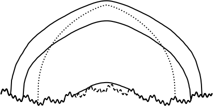
Within a Stokes-based theory the shape that should be predicted for a glacier’s grounded margin is not so clear (Figure 3). This situation makes it difficult to determine a Sobolev space in which VI problem (46) might be well-posed. The SIA theory suggests root-type (fractional-power) shapes for the marginal surface elevation, with different shapes for advance and retreat, but with unbounded gradients in all known cases [9, 26]. By contrast, a “wedge” margin shape with a bounded gradient has been hypothesized [14, for example], which would allow .
Reality is of course more complicated. In the vicinity of an ice margin, especially on steep bedrock features, real glacier ice can generate overhangs which violate the assumption of a single-valued surface elevation function. Similarly, real bedrock can overhang. Fractures, crevasses, and cliffs are commonly found in glacier margins, but modeling such features requires a departure from the viscous fluid paradigm considered here.
Because margins are small features compared to the overall scale of glaciers and ice sheets, most modeling literature ignores overhangs and assumes instead that surface and bed elevation functions are well-defined; see [25, 27, 33, 42] among many examples. Extending Stokes-based viscous models by allowing fractures, for example by supplementing momentum conservation with an additional advected damage variable [39] so that ice-cliff calving can occur via a stress-failure criterion, might one day suggest a preferred margin regularity assumption for a viscous-only theory like the one here.
4.4 Conjectural well-posedness for the continuum problem
Subsections 4.1–4.3 have deployed various imperfect arguments to explain why the backward Euler VI problem (46) could be well-posed, or at least why other approaches are less promising. We now state a mathematically-precise conjectural framework for well-posedness of this problem based upon the idea that the surface motion map assigns different results to inputs which differ in Sobolev norm, and indeed that it does so in a positive manner.
Conjecture 4.1.
Inequality (54) is called q-coercivity of over . In the abstract context of Section 6, if an operator is both continuous and q-coercive, over a closed and convex subset of a Banach space, then the corresponding VI problem is well-posed. This is what we prove next, namely that Conjectures 3.3 and 4.1 are sufficient for well-posedness of implicit time step VI problem (46).
Theorem 4.2.
Proof 4.3.
Let . By Lemma 3.4 there is so that if then . Then by definition (45), Hölder’s inequality, and Sobolev’s inequality we have
| (55) | ||||
for some which depends on and . Thus is (Lipschitz) continuous on bounded subsets of . If Conjecture 4.1 holds then
| (56) | ||||
so is q-coercive over with constant . From definition (25), the hypothesis on , and Hölder’s inequality,
| (57) |
for all . Because by Sobolev’s inequality, and , it follows that . Because is q-coercive it is also coercive and strictly-monotone (Definition 6.1). Now Corollary III.1.8 of [30] shows unique existence of a solution to (46).
Note that if the surface motion map has coercivity constant (Conjecture 4.1) then has constant .
Theorem 4.2 addresses only the well-posedness of a single time-step problem over . Its conclusion is not sufficient to show well-posedness of the time-dependent problem parabolic VI problem over corresponding to NCP (3). If this problem were known to be well-posed then one might analyze whether implicit steps converge in the limit.
The computation of and , or equivalent expressions, would seem to be necessary in any evolving-geometry Stokes framework. These expressions are addressed in Conjectures 3.3 and 4.1, and it would seem that any modeling practitioner who uses Stokes dynamics would expect such expressions to be well-behaved in some manner. However, the Conjectures may be difficult to prove despite some progress in Sections 2 and 3. Greater progress has been made in the SIA case [10, 26, 37], which could be helpful.
5 Numerical exploration of coercivity
We may explore the validity of Conjecture 4.1 by sampling from numerical simulations. The experiments here,666Source code is at the public repository github.com/bueler/glacier-fe-estimate, in the py/ directory. The codes call the library at github.com/bueler/stokes-extrude. performed using Python and the Firedrake FE library [24], are not intended to demonstrate implicit time-stepping, but only to generate admissible surface elevation pairs to use as samples. For a given sample pair we evaluated the -coercivity ratio
| (58) |
If, for all pairs in some , the set of ratios were bounded below by a positive constant , then this would confirm the coercivity inequality (54) for that . Of course, a numerical experiment allows only finite sampling, and furthermore a finite spatial discretization must be used.
The domain for our experiments is the 1D interval , km, with . The interval was uniformly-meshed into equal intervals. The piecewise-linear FE space was used for the bed and the surface , giving polygonal domains defined by ; see equation (1). Three bed profiles (Figure 4) were considered, flat with , smooth with a superposition of several wavelengths down to 10 km, and rough with an additional 4 km wavelength mode. These beds generate corresponding constraint sets , .
For each constraint set , three constant SMB values were considered (units ): . For each SMB value a time-dependent run of duration years started from the same initial surface elevation profile.777A Halfar profile [23] with characteristic time years was used as the initial state. In the case of a flat bed and the exact time-dependent solution under SIA dynamics is known by Halfar’s result [23]. The final ( a) surface elevation, from using Stokes dynamics in the actual experiment, agrees closely with the SIA exact solution; compare comments in [33]. The positive SMB value was sufficient to advance the ice margins nearly to the domain boundary at by the final time , while the negative SMB value caused the glacier to disappear entirely by that time.
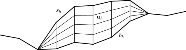
In these simulations each time-step VI (46) was semi-implicit. That is, definition (45) was modified to use the prior surface velocity . The numerical VI solution was by a reduced-space Newton method with line search [4]. The “FSSA” stabilization technique from [33] was applied, which generates a modified Stokes weak form compared to (12); see equation (23) in [33]. The Stokes problem (12), with viscosity regularization in (5), was solved on each domain using a vertically-extruded mesh of quadrilaterals (Figure 7), mixed FE method for the (Taylor-Hood) stable pair [15], and a Newton solver, with direct solution of the linear step equations. The resulting time-dependent numerical method is only conditionally stable, but adequate for our purpose of generating sample surfaces.
The basic result of these experiments is shown in Figure 5. These are sample ratio histograms from the highest spatial resolution, namely m and 40 elements in each extruded column. More than of all the ratios were positive, and of these the medians for the three were in the range . For the remaining negative ratios, the medians were in the range , much smaller in magnitude.
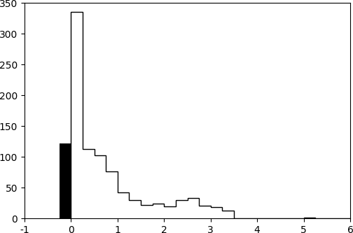
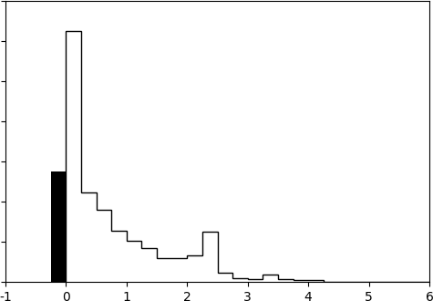
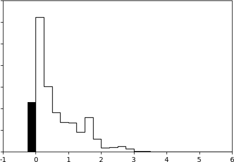
Figure 5 does not represent compelling evidence of -coercivity by definition (61), but it does not exclude it. In fact, the details of the discretization of the ice margin strongly influence the negative ratios. Noting that ratio evaluation uses integral (38), if that integrand is reset to zero where the ice is thinner than 100 m then the negative values disappear (not shown). Even without such thresholding, at lower horizontal resolution ( m) the median magnitude of negative ratios was roughly twice as large (not shown). The disappearance of negative ratios under grid refinement should not be excluded. Margin approximation improvements, such as adaptive/local mesh refinement, will probably improve the numerical evidence for coercivity.
It is theoretically possible that the operator is monotone, inequality (60), but not q-coercive for any q. In that case a revised well-posedness argument can be attempted, for example by adding a small coercive form as in section III.2 of [30]. However, if a continuum pair with a negative ratio were actually to be found in some , i.e. with an exact continuum ratio from (58), then the coercivity-based well-posedness framework of this paper would fail.
Regarding Conjecture 3.3, Lipschitz continuity for the surface velocity trace, the ratio for the same sample pairs was also evaluated. Over all three sets , at the highest resolution, the maximum ratio was , providing a lower bound for . Again, numerical experiments obviously cannot prove the Conjecture.
6 Abstract error estimate for a finite element approximation
In this Section we consider the FE approximation of an abstract VI problem. We will return to glaciological problem (46) in Section 7.
Let be a real reflexive Banach space with norm and topological dual (Banach) space . Denote the dual pairing of and by , and define . Let be a nonempty, closed, and convex subset, called the constraint set, whose elements are called admissible. For a continuous, but generally nonlinear, operator , and a source functional , the VI problem is to find such that
| (59) |
VI problem (46) is in this form. The best known example of (59) is the obstacle problem for the Laplacian operator—see [12, 16, 30] for theory and FE analysis. A key observation is that is generally nonzero when solves (59), though if is in the interior of then . Under sufficient regularity assumptions an NCP like (3) or (7) follows from (59).
Definition 6.1.
If is monotone and coercive, and also continuous on finite-dimensional subspaces, then VI (59) has a solution [30, Corollary III.1.8]. If is strictly monotone then the solution is unique. The definition of q-coercive was already given in Conjecture 4.1. If is q-coercive then it coercive and strictly monotone, so q-coercivity and continuity yield well-posedness for (59). Note that Definitions 6.1 and 6.2 do not require to be defined on all of , but only on .
The following definition appeared in Lemma 3.4. If it holds then is continuous.
Definition 6.2.
For let . We say is Lipshitz on bounded subsets of if for every there is so that if and then , equivalently
| (62) |
An FE method for (59) becomes a finite-dimensional VI problem. Suppose is a finite-dimensional subspace, typically some space of continuous, piecewise-polynomial functions defined on a mesh. The FE constraint set is assumed to be closed and convex, but generally . Let , and note that generally because of quadrature and other approximations. (Looking ahead, both and occur naturally in the glacier geometry problem; see Section 7.) The FE VI problem is
| (63) |
We will assume that (63) has a solution .
The following abstract error estimation theorem extends the well-known result by Falk [18]. See also Theorem 5.1.1 in [12], and a version of the estimate wherein (but not ) solves a variational equality [31, Theorem 1]. For the proof we must assume that the domain of includes the FE solution, which is achieved here by defining a convex superset of and . This technical assumption permits a clean and general estimation theorem, but the choice of made in Section 7 means that the convex hull construction is not needed in our glacier application; see Corollary 6.5.
Theorem 6.3.
Define to be the closure in of the convex hull of , and suppose that . For , with conjugate exponent , assume that is q-coercive over with constant , and Lipshitz on bounded sets of . Suppose solves (59) and solves (63), and let . Then there is a constant , not otherwise depending on or , so that
| (64) | ||||
Proof 6.4.
For arbitrary and , rewrite (59) and (63) as follows:
| (65) | ||||
It follows from (65) and the q-coercivity of that
| (66) | ||||
Since , by the Lipshitz assumption over there is so that
| (67) |
Noting , now use Young’s inequality with [16, Appendix B.2]:
| (68) | ||||
where . Choose so that , and subtract:
| (69) | ||||
Take infimums to show (64).
Note that Theorem 6.3 does not assume any of the following: , is linear, , is continuous, or is q-coercive. We also do not require that is the unique solution of (63); the result holds for any solution.
The next Corollary addresses two important cases where the convex hull operation is not needed. We will see in Section 7 that case i) can be imposed in glacier simulations.
Corollary 6.5.
Suppose that one of the following situations apply:
-
i)
, or
-
ii)
is defined on all of .
Assume is q-coercive on, and Lipschitz on bounded subsets of, its domain, namely or , respectively. Otherwise make the assumptions of Theorem 6.3. Then conclusion (64) holds. Additionally, in case i) the “ ” term is zero.
Consider . It might be a measure or a measurable function, and then the first two terms in estimate (64) preserve information about its support. (This plays a role in the glacier application of Section 7.) By contrast, the Hilbert space result in [18] computes norms and loses this information. The following Corollary, with easy proof, takes such a norm-based approach. We suppose that continuously and densely embeds into a larger Banach space :
| (70) |
Observe that . A standard example is and .
Corollary 6.6.
The result by Falk [18] combines the above two Corollaries, under the further assumptions that is linear and . To say this precisely, suppose is bilinear, uniformly elliptic, and continuous on a Hilbert space . (The definition of uniformly elliptic coincides with definition (61) of -coercive, and continuity of implies (62).) Suppose that and for some Hilbert space , and that so that, up to isomorphism, . Finally, suppose that . Then case ii) of Corollary 6.5 combines with Corollary 6.6 to yield Theorem 1 in [18].
The term in estimates (64) and (71) is generally nonzero in obstacle problems where . To see how this case can occur, consider a unilateral obstacle problem where . Suppose is the FE interpolant of , and define . While for interpolation nodes , generally will not hold for all even if is arbitrarily smooth, nor will hold (Figure 6, left; see also [12, Figure 5.1.3]).
For such unilateral problems we may bypass the issue by using a monotone nodal operator (Figure 6, right), defined as follows. Assume elements and a continuous obstacle . For a given triangulation and node let
| (72) |
where is the closure of the union of the elements adjacent to ; compare the multilevel version of in [8]. Let be the unique function with nodal values . Then for all .
When we return to the surface elevation based glacier problem in Section 7 we will use this monotone operator on the bed elevation. Models which solve for ice thickness using elements do not need this step; here , so holds.
The following Corollary collects some conclusions one might draw from assuming , and making further assumptions, especially that . Note that (75) is Cea’s lemma [12, Theorem 2.4.1] in a Banach space. This PDE case, with no active set or free boundary, applies in the glacier context only when the entire domain is covered in ice.
7 Application of the theory to numerical glacier models
Now we can synthesize the theory and apply it to an implicit time step of a Stokes-based glacier simulation. This will give the phrase “conforming FE method” a precise meaning for such glacier simulations. We will combine three previous threads: i) well-posedness and a priori bounds for the glaciological Stokes problem on a fixed domain (Section 2), ii) conjectural well-posedness theory of the surface elevation VI problem (Sections 3 and 4), and iii) the abstract error estimate for FE solutions of VIs (Section 6).
Consider an FE method for VI problem (46). For a finite-dimensional subspace , with a constraint set , we seek solving
| (76) |
The operator denotes an FE approximation to the operator defined in (45). The source is defined exactly as before, by equation (25). We assume that is general; we do not require .
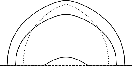
Evaluation of in the FE VI problem (76) requires the nontrivial numerical solution of a glaciological Stokes problem (12) over a 3D mesh of the domain between and (Figure 7). Such a mesh need not be extruded vertically as shown, nor must necessarily be piecewise-linear, but the upper and lower surfaces, where boundary conditions (6c) and (6d) are applied, must be admissible FE functions, i.e. with . The numerical velocity from solving the Stokes problem, over the domain geometry defined by , is denoted , and its surface trace is denoted . Observe that will generally be different from the surface trace of the exact solution of the same Stokes boundary value problem for the same () geometry, denoted by . Technically, the FE operator is defined as
| (77) |
for . This is a different operator from , defined in (45), because it uses the numerical solution velocity and not the exact velocity.
A key concern in applying abstract Theorem 6.3 or its Corollaries in a glaciological context is the choice of the numerical bed elevation , which defines the constraint set . We will assume that is continuous on the closed domain . (An abstract can indeed be considered, but in practice is provided via a high resolution map derived from ice-penetrating radar [35]. It may already be in a continuous FE space, but often on a finer mesh.) We assert that it is better to choose to satisfy . A monotone nodal operator (72), or similar, can be applied, . As one would in “conforming” FE methods for PDE problems [15], we will also assume along the fixed boundary .
Define an interpolation and truncation operation as follows. For this gives the unique FE function so that
| (78) |
for every interior node , with if . Observe that definition (78) only yields nodal admissibility. The FE space must be such that this implies admissibility per se, namely that for all , so that . This condition is satisfied by the continuous and piecewise-linear FE space , but not, for example, by [8], but compare the higher-order approach taken in [29].
Collecting the above assumptions, from now on we make these standard assumptions for solving VI problem (46) using numerical scheme (76).
Standard Assumptions.
The following data are given:
-
1.
A bounded, convex polygon .
-
2.
An exponent , with conjugate exponent .
-
3.
A time-dependent SMB function .
-
4.
A bed topography function , with piecewise-linear boundary values .
We make these definitions:
-
5.
, with the norm as defined in (31).
-
6.
.
-
7.
denotes a finite-dimensional and conforming FE space, from a mesh exactly tiling .
The following are assumed to hold:
-
8.
Conjecture 3.3, with Lipschitz constant .
-
9.
Conjecture 4.1, with exponent and coercivity constant .
We also assume and define:
-
10.
is given, with on and along .
-
11.
.
-
12.
Interpolation/truncation yields admissible elements in .
The conforming condition follows from assumptions 10 and 11, with advantages to follow. As seen in the proof of Theorem 4.2, assumptions 8 and 9 show that is q-coercive and Lipschitz on bounded subsets of . By Theorem 4.2 and case i) of Corollary 6.5 we have the following Lemma.
Lemma 7.1.
Each term in estimate (79) turns out to have a clear glaciological meaning, which we expose in the following Theorem. Recall that is the velocity space for the Stokes problem (12), denotes the maximum diameter of cells in , and denotes the 3D domain defined by , denotes the trace constant of that domain (Lemma 2.6).
Theorem 7.2.
Before proving the Theorem we sketch the meaning of each term; more detail appears after the proof.
-
term 1:
This term comes from FE approximation of the bed in the ice-free area . If the bed were exactly representable () then it would be zero. Note that in the ice-free area , so the factor in the integrand reflects the smallest possible difference . Also (Section 3) so the integrand is nonnegative.
-
term 2:
This term quantifies how numerical errors in solving the Stokes problem, over the domain , will affect the geometrical error in .
- term 3:
Proof 7.3.
Because solves (46), the residual , while generally nonzero, is non-negative. In particular, if is nonnegative then and . Thus is a non-negative distribution, and so it is represented by a positive Borel measure [32, Theorem 6.22], that is, . However, by the proof of Theorem II.6.9 in [30] this measure is supported in and has density . (Recall from Section 3 that on .)
Apply Lemma 7.1. Note that and on . From the first term in (79) we now get term 1 when we set :
| (83) |
Consider the second term in (79). Recall that is the surface area element for the surface . After definitions (45) and (77), apply the triangle and Hölder inequalities:888A similar argument was used in the proof of Lemma 3.1.
| (84) | ||||
Now apply the trace inequality (Lemma 2.6) and use the fact that if :
| (85) | ||||
Recalling norm definition (31), we have term 2.
Term 3 follows by substituting into the third term in (79).
Regarding term 1, consider those portions of which are also ice-free according to the FE solution, namely points where . In such areas generally , for example because of the monotone restriction used for assumption 10. This implies that there is a positive “fake ice thickness” error for the FE solution, namely , but the numerical model reports zero thickness (). In areas of strong ablation, and far from the nearest flowing glacier, one might simply declare that such “fake ice” does not represent an FE-generated error, and then the magnitude of term 1 can be reduced accordingly, by excluding obviously ice-free areas from the integral. However, generally is unknown, and therefore such exclusion is not appropriate, nor implementable, near the unknown free boundary . A climate which puts the bed elevation near the equilibrium line altitude [22] in any ice-free area would also make such casual exclusion of a potentially real FE error unwise.
Note that a time-stepping FE solution of any fluid-layer VI problem like (46) commits a mass conservation error near the (unknown) exact free boundary even when there is no difference between the exact and FE obstacles. The mass conservation barrier theory in [6] addresses this concern, in terms of the fluid layer thickness. (For thicknesses the obstacle is the zero function; it has an exact FE representation.) While the theory in [6] applies here as well, term 1 in bound (81) is novel relative to the various mass-conservation errors identified there. (See in [6]: retreat loss, boundary leak, and cell slop.)
The Stokes velocity error norm in term 2 of (81) describes the error in solving problem (12) on a particular (“fixed”) 3D domain . One may use reasonable assumptions and existing techniques to derive a convergence rate for this term if one supposes counter-factually that does not change under mesh refinement. The following sketch does this; it is from [28, Theorem 4.9]; see also the FE theory for linear Stokes in [15], for example. One assumes solution regularity for the Stokes problem (12), specifically that and for some . The mixed FE method for (12) is assumed to satisfy Bramble-Hilbert type interpolations bounds in and for the discrete velocity and pressure spaces, respectively; see [28, inequalities (4.26), (4.27)]. Finally one assumes that the mixed FE method satisfies a discrete inf-sup condition [28, equation (4.1)]. One then concludes that
| (86) |
for a constant which depends on the regularity norms of , the discrete inf-sup constant, and the domain . To apply such a technique to VI problem (46), via Theorem 7.2, one would at least need to prove two bounds, First, one would need a bound showing the regularity of the solution of (12), over the domain , when ; this extends Conjecture 3.3. Second, seemingly more difficult and not remotely attempted here, one must bound how the constant in (86) depends on the properties of .
One might also try to bound term 3 in (81) via estimates for FE interpolation. From [12, Theorem 3.1.6], for example, if then there is , depending only on the finite element family for , so that for all ,
| (87) |
Here is the ordinary interpolation into , not including truncation into as with operation (78). For simplicity suppose we somehow arrange that , thus that . Now suppose that the exact solution of VI problem (46) also satisfies for some . Then it follows that term 3 in (81) is with a coefficient that depends on the norm of . (Compare the argument for [26, Theorem 4.3], which makes a comparably strong regularity assumption for a power of the thickness function, but in an SIA problem.)
However, the sketch in the previous paragraph is a fantasy. The hypothesis that is too strong even if the data entering into VI problem (46) are arbitrarily smooth. It is true that in classical obstacle problems the solution is generically tangential along the free boundary, which permits such regularity [30, Chapter IV]. However a glacier’s surface gradient need not approach the bed gradient at points along the ice margin (Subsection 4.3). While is credible, is not, which means that such direct use of interpolation theory to prove convergence is unlikely to work.
8 Discussion and conclusion
The major result of this paper is Theorem 7.2, which bounds the numerical surface elevation error when a glacier is modeled using non-shallow Stokes dynamics. The bound, inequality (81), only estimates the FE error made in a single implicit time step, namely VI problem (46). The first two terms in the bound can be reduced by improving bed elevation interpolation, and by solving the Stokes problem more accurately, respectively. However, the surface elevation solution to (46) must be expected to have low regularity, especially across the ice margin (free boundary). Near-margin mesh refinement may be the only technique which reduces the FE interpolation/truncation error in the surface elevation, which is the third and final term in the bound.
However, the results here leave us far from an FE convergence proof for the main time-evolution problem of glaciology. This problem is written in the Introduction; it combines NCP (3) coupled with the Stokes problem (5)–(6). It is a parabolic VI [20], on which analysis is generally more difficult than for the (roughly) elliptic single-step VI problem (46). Turning Theorem 7.2 into a convergence proof would therefore be a major step requiring a significantly-extended theory; see the end of Section 7.
Neither do we have a proof of the well-posedness of the continuous-space, implicit-step problem (46) itself. Much of the current paper is devoted to conjecturing such well-posedness (Sections 3–5). The abstract FE bound in Theorem 6.3 applies to problem (46) because of Theorem 4.2, an immediate consequence of Conjectures 3.3 and 4.1. Our attempt at least clarifies which properties of the surface motion part of the surface kinematical equation—actually an NCP or VI problem—need to hold if we seek such well-posed time steps in a non-shallow glacier model.
The root of the matter is coercivity of this surface motion, namely Conjecture 4.1. A strategy for proving this Conjecture is not clear to this author. A weaker version of the Conjecture comes from setting for supported where . That is, one would consider admissible perturbations of the glacier surface which do not move the glacier margin. This may be easier to prove, but it is not sufficient for Theorem 4.2, and it does not address the marginal shape and overhang issues discussed in Section 4. On the other hand, one might modify or regularize the operator definition (45) in some manner, e.g. by adding an elliptic regularization. Our numerical evidence for coercivity of the existing operator, from a very basic numerical approach, is quite weak (Section 5), but in a regularized model the near-margin numerical approximation might be easier.
References
- [1] D. Acheson, Elementary Fluid Dynamics, Oxford University Press, 1990.
- [2] U. Ascher and L. Petzold, Computer Methods for Ordinary Differential Equations and Differential-algebraic Equations, SIAM Press, Philadelphia, 1998.
- [3] A. Aschwanden, E. Bueler, C. Khroulev, and H. Blatter, An enthalpy formulation for glaciers and ice sheets, Journal of Glaciology, 58 (2012), pp. 441–457, https://doi.org/10.3189/2012JoG11J088.
- [4] S. Benson and T. Munson, Flexible complementarity solvers for large-scale applications, Optimization Methods and Software, 21 (2006), pp. 155–168, https://doi.org/10.1080/10556780500065382.
- [5] D. Boffi, F. Brezzi, and M. Fortin, Mixed Finite Element Methods and Applications, vol. 44, Springer, 2013.
- [6] E. Bueler, Conservation laws for free-boundary fluid layers, SIAM J. Appl. Math., 81 (2021), pp. 2007–2032, https://doi.org/10.1137/20M135217X.
- [7] E. Bueler, Performance analysis of high-resolution ice-sheet simulations, J. Glaciol., 69 (2023), pp. 930–935, https://doi.org/10.1017/jog.2022.113.
- [8] E. Bueler and P. Farrell, A full approximation scheme multilevel method for nonlinear variational inequalities, SIAM J. Sci. Comput., 46 (2024), pp. A2421–A2444, https://doi.org/10.1137/23M1594200.
- [9] E. Bueler, C. S. Lingle, J. A. Kallen-Brown, D. N. Covey, and L. N. Bowman, Exact solutions and verification of numerical models for isothermal ice sheets, J. Glaciol., 51 (2005), pp. 291–306, https://doi.org/10.3189/172756505781829449.
- [10] N. Calvo et al., On a doubly nonlinear parabolic obstacle problem modelling ice sheet dynamics, SIAM Journal on Applied Mathematics, 63 (2003), pp. 683–707, https://doi.org/10.1137/S0036139901385345.
- [11] G. Cheng, P. Lötstedt, and L. von Sydow, Accurate and stable time stepping in ice sheet modeling, J. Comput. Phys., 329 (2017), pp. 29–47, https://doi.org/https://doi.org/10.1016/j.jcp.2016.10.060.
- [12] P. Ciarlet, The Finite Element Method for Elliptic Problems, SIAM Press, Philadelphia, 2002. Reprint of the 1978 original.
- [13] J. Cogley, R. Hock, L. Rasmussen, A. Arendt, A. Bauder, R. Braithwaite, P. Jansson, G. Kaser, M. Möller, L. Nicholson, and M. Zemp, Glossary of glacier mass balance and related terms, IHP-VII Technical Documents in Hydrology 86, UNESCO-IHP, Paris, 2011.
- [14] K. A. Echelmeyer and B. Kamb, Stress-gradient coupling in glacier flow: II. Longitudinal averaging in the flow response to small perturbations in ice thickness and surface slope, J. Glaciol., 32 (1986), pp. 285–298, https://doi.org/10.3189/S0022143000015616.
- [15] H. C. Elman, D. J. Silvester, and A. J. Wathen, Finite Elements and Fast Iterative Solvers: with Applications in Incompressible Fluid Dynamics, Oxford University Press, Oxford, UK, 2nd ed., 2014.
- [16] L. C. Evans, Partial Differential Equations, Graduate Studies in Mathematics, American Mathematical Society, Providence, 2nd ed., 2010.
- [17] F. Facchinei and J.-S. Pang, Finite-Dimensional Variational Inequalities and Complementarity Problems, vol. 1, Springer, 2003.
- [18] R. S. Falk, Error estimates for the approximation of a class of variational inequalities, Mathematics of Computation, 28 (1974), pp. 963–971.
- [19] D. Gilbarg and N. S. Trudinger, Elliptic Partial Differential Equations of Second Order, Springer-Verlag, Berlin, reprint of the 1998 ed., 2001.
- [20] R. Glowinski, Numerical Methods for Nonlinear Variational Problems, Springer-Verlag, Berlin, 1984.
- [21] D. L. Goldsby and D. L. Kohlstedt, Superplastic deformation of ice: experimental observations, J. Geophys. Res., 106 (2001), pp. 11017–11030, https://doi.org/10.1029/2000JB900336.
- [22] R. Greve and H. Blatter, Dynamics of Ice Sheets and Glaciers, Advances in Geophysical and Environmental Mechanics and Mathematics, Springer, Berlin, Germany, 2009.
- [23] P. Halfar, On the dynamics of the ice sheets, J. Geophys. Res., 86 (1981), pp. 11065–11072, https://doi.org/10.1029/JC086iC11p11065.
- [24] D. A. Ham, P. H. J. Kelly, L. Mitchell, C. J. Cotter, R. C. Kirby, K. Sagiyama, N. Bouziani, S. Vorderwuelbecke, T. J. Gregory, J. Betteridge, D. R. Shapero, R. W. Nixon-Hill, C. J. Ward, P. E. Farrell, P. D. Brubeck, I. Marsden, T. H. Gibson, M. Homolya, T. Sun, A. T. T. McRae, F. Luporini, A. Gregory, M. Lange, S. W. Funke, F. Rathgeber, G.-T. Bercea, and G. R. Markall, Firedrake User Manual, Imperial College London and University of Oxford and Baylor University and University of Washington, first edition ed., 5 2023, https://doi.org/10.25561/104839.
- [25] T. Isaac, G. Stadler, and O. Ghattas, Solution of nonlinear Stokes equations discretized by high-order finite elements on nonconforming and anisotropic meshes, with application to ice sheet dynamics, SIAM J. Sci. Comput., 37 (2015), pp. B804–B833, https://doi.org/10.1137/140974407.
- [26] G. Jouvet and E. Bueler, Steady, shallow ice sheets as obstacle problems: well-posedness and finite element approximation, SIAM J. Appl. Math., 72 (2012), pp. 1292–1314, https://doi.org/10.1137/110856654.
- [27] G. Jouvet, M. Picasso, J. Rappaz, and H. Blatter, A new algorithm to simulate the dynamics of a glacier: theory and applications, J. Glaciol., 54 (2008), pp. 801–811, https://doi.org/10.3189/002214308787780049.
- [28] G. Jouvet and J. Rappaz, Analysis and finite element approximation of a nonlinear stationary Stokes problem arising in glaciology, Advances in Numerical Analysis, (2011), https://doi.org/10.1155/2011/164581.
- [29] B. Keith and T. M. Surowiec, Proximal Galerkin: A structure-preserving finite element method for pointwise bound constraints, arXiv preprint arXiv:2307.12444, (2023), https://doi.org/10.48550/arXiv.2307.12444.
- [30] D. Kinderlehrer and G. Stampacchia, An Introduction to Variational Inequalities and their Applications, Academic Press, New York, 1980.
- [31] R. C. Kirby and D. Shapero, High-order bounds-satisfying approximation of partial differential equations via finite element variational inequalities, Numerische Mathematik, 156 (2024), pp. 927–947, https://doi.org/10.1007/s00211-024-01405-y.
- [32] E. H. Lieb and M. Loss, Analysis, vol. 14 of Graduate Studies in Mathematics, American Mathematical Society, Providence, 1997.
- [33] A. Löfgren, J. Ahlkrona, and C. Helanow, Increasing stable time-step sizes of the free-surface problem arising in ice-sheet simulations, Journal of Computational Physics: X, 16 (2022), https://doi.org/10.1016/j.jcpx.2022.100114.
- [34] G. J. Minty, On a “monotonicity” method for the solution of nonlinear equations in Banach spaces, Proceedings of the National Academy of Sciences, 50 (1963), pp. 1038–1041, https://doi.org/10.1073/pnas.50.6.1038.
- [35] M. Morlighem et al., BedMachine v3: Complete bed topography and ocean bathymetry mapping of Greenland from multibeam echo sounding combined with mass conservation, Geophysical Research Letters, 44 (2017), pp. 11051–11061, https://doi.org/10.1002/2017GL074954.
- [36] F. Pattyn, L. Perichon, et al., Benchmark experiments for higher-order and full-Stokes ice sheet models (ISMIP–HOM), The Cryosphere, 2 (2008), pp. 95–108, https://doi.org/10.5194/tc-2-95-2008.
- [37] P. Piersanti and R. Temam, On the dynamics of grounded shallow ice sheets: Modeling and analysis, Advances in Nonlinear Analysis, 12 (2023), https://doi.org/10.1515/anona-2022-0280.
- [38] W. Pompe, Korn’s first inequality with variable coefficients and its generalization, Commentationes Mathematicae Universitatis Carolinae, 44 (2003), pp. 57–70.
- [39] A. Pralong and M. Funk, Dynamic damage model of crevasse opening and application to glacier calving, J. Geophys. Res.: Solid Earth, 110 (2005), https://doi.org/https://doi.org/10.1029/2004JB003104.
- [40] C. Schoof and I. J. Hewitt, Ice-sheet dynamics, Annual Review of Fluid Mechanics, 45 (2013), pp. 217–239, https://doi.org/10.1002/jgrf.20146.
- [41] R. Winkelmann, M. A. Martin, M. Haseloff, T. Albrecht, E. Bueler, C. Khroulev, and A. Levermann, The Potsdam Parallel Ice Sheet Model (PISM-PIK) Part 1: Model description, The Cryosphere, 5 (2011), pp. 715–726, https://doi.org/10.5194/tc-5-715-2011.
- [42] A. Wirbel and A. Jarosch, Inequality-constrained free-surface evolution in a full Stokes ice flow model (evolve_glacier v1.1), Geoscientific Model Development, 13 (2020), pp. 6425–6445, https://doi.org/10.5194/gmd-13-6425-2020.