Analysis of Clustering and Degree Index in Random Graphs and Complex Networks

Abstract

The purpose of this paper is to analyze the degree index and clustering index in random graphs. The degree index in our setup is a certain measure of degree irregularity whose basic properties are well studied in the literature, and the corresponding theoretical analysis in a random graph setup turns out to be tractable. On the other hand, the clustering index, based on a similar reasoning, is first introduced in this manuscript. Computing exact expressions for the expected clustering index turns out to be more challenging even in the case of Erdős-Rényi graphs, and our results are on obtaining relevant upper bounds. These are also complemented with observations based on Monte Carlo simulations. Besides the Erdős-Rényi case, we also do simulation-based analysis for random regular graphs, the Barabási-Albert model and the Watts-Strogatz model.

1 Introduction

Since the introduction of Erdős-Rényi graphs around 1960 ([7], [8]), random graphs gained substantial importance in both applied and theoretical fields. Meanwhile, various statistics of interest for the underlying networks (or, graphs) have been studied, which include the average degree, clustering coefficient, efficiency, and modularity, among several others. See, for example, [6], [12], [14] and [20] for relevant definitions and certain applications. Due to the development of graph-based machine learning algorithms in recent years, these statistics have been even more popular, especially in classification problems [21]. The purpose of this paper is to study two other types of graph characteristics in random graphs.

In order to describe the two characteristics we study, let $\mathcal{G}=(V,E)$ be a graph where $V=\{1,2,\ldots,n\}$ for some $n\in\mathbb{N}$. Let $N(k)$ be the set of neighbors of $k\in V$ in $\mathcal{G}$. We denote the degree of $k$ by $d_{k}$. With this notation, we define the $\alpha$-level degree index of $\mathcal{G}$ to be

$$\mathrm{DI}_{\alpha}(\mathcal{G})=\sum_{1\leq i<j\leq n}|d_{i}-d_{j}|^{\alpha}.$$

Here, $\alpha>0$ is a real number which is chosen to be in $\{1,2\}$ in this manuscript. Also let us note that $\sum_{i<j}$ will mean $\sum_{1\leq i<j\leq n}$ below.

The second graph characteristic of interest for us will be the clustering index, which, as far as we know, is not studied previously in the literature. First, recall that for given $i\in V$, when $d_{i}\geq 2$, the local clustering coefficient of $i$ is defined to be

$$C(i)=\frac{1}{d_{i}(d_{i}-1)}\sum_{j,k\in N(i):j\neq k}\mathbf{1}(j\leftrightarrow k).$$

In case where $d_{i}\in\{0,1\}$, we set $C(i)=0$. Now, similar to the degree index, for $\alpha>0$, we define the $\alpha$-level clustering index of $\mathcal{G}$ to be

$$\mathrm{CI}_{\alpha}(\mathcal{G})=\sum_{i<j}|C(i)-C(j)|^{\alpha}.$$

Here again $\alpha$ in our case is either 1 or 2. In the upcoming sections, we will analyze both $\mathrm{DI}_{\alpha}(G)$ and $\mathrm{CI}_{\alpha}(G)$ when $G$ is an Erdős-Rényi graph. We will complement these by doing observations on other random graph models.

The clustering index is a measure that provides certain information about the uniformity among the local neighborhood structure of $\mathcal{G}$ by focusing on the clustering. As already noted, although such a coefficient is quite natural to define, it is first introduced in this manuscript to the best of our knowledge. That said, the degree index defined above is previously studied in the literature in distinct contexts. Our primary goal in this paper is to analyze these two indices for the case of Erdős-Rényi graphs. For such random graphs, the degree index case turns out to be relatively straightforward, and precise formulas for the expected degree index are obtainable. On the other hand, the case of the clustering index is more involved, and we are not able to obtain exact formulas. However, we show that when $\mathcal{G}$ is an Erdős-Rényi graph with $n$ nodes and a fixed attachment probability $p$, the bounds

$$\mathbb{E}[\mathrm{CI}_{1}(\mathcal{G})]\leq K_{1}n$$

and

$$\mathbb{E}[\mathrm{CI}_{2}(\mathcal{G})]\leq K_{2},$$

hold for every $n$, where $K_{1},K_{2}$ are constants depending on $p$, but not on $n$. Our heuristic arguments yield that matching lower bounds are also true for both cases, but we have not verified these rigorously yet.

Let us now give some pointers for previous work on the degree index, and then include some discussions and references on the clustering coefficient. Noting that $\mathrm{DI}_{\alpha}(\mathcal{G})=0$ means that the graph under study is regular, this quantity is considered as a measure of irregularity of the graph [22]. An irregularity definition that has found significant use in the literature is the Albertson index introduced in [5], in which the corresponding definition is similar to ours, but the sum under consideration is over the edge set instead of the vertices. Although the irregularity used in the present manuscript is quite natural to consider, the special case $\mathrm{DI}_{1}(\mathcal{G})$ was relatively recently introduced in [1], where the authors call it the total irregularity of the graph. Also, a form of the special case of $\mathrm{DI}_{2}(\mathcal{G})$ in which the corresponding sum is over the edge set instead of the node was proposed in [2]. Aside from these, there are other notions of graph degree irregularity, see [3] for a partial list.

The clustering coefficient of a node $i\in V(\mathcal{G})$ is a measure of the likeliness of neighbors of $i$ to be neighbors among themselves [23]. The clustering coefficient is extensively studied in the literature, and several variations and generalizations are proposed; see [15], [16] and [17] for some exemplary work. The clustering coefficient is also studied in a random graph setup. For instance, [24] analyzes the clustering coefficient in Erdős-Rényi graphs and certain random regular graphs. [9] does an investigation in the case of a generalized small world model. On the other hand, [17] discusses a natural generalization of the standard clustering coefficient, and analyzes in both Erdős-Rényi and small world settings.

Here is a summary of the contributions of the current manuscript. The degree index we study is well known in the literature, but it is not analyzed for random graphs to the best of our knowledge. Here we are able to fully understand the expected degree index for $\alpha\in\{1,2\}$. We are not aware of any work on clustering index in the literature. After introducing this concept, we prove related results on the expected clustering index for Erdős-Rényi graphs, and in particular we obtain upper bounds for this quantity for $\alpha\in\{1,2\}$. Although the theoretical work is done for the Erdős-Rényi due to its simplicity, we complement this with a simulation study on other random graph models.

The rest of the paper is organized as follows. Next section contains some basic observations on the clustering index, which can be easily adapted to the degree index. This section also includes a brief discussion on the comparison of the extremal cases of the degree index and the clustering index. Afterwards, in Section 3 we analyze the clustering index in Erdős-Rényi graphs, and provide upper bounds for the expected clustering index for both $\alpha=1$ and $2$. Later, in Section 4, a similar study is done for the degree index. Section 5 is then devoted to a simulation based study for the indices under study for random regular graphs, Barabási-Albert model and Watts-Strogatz model. Lastly, we conclude the paper in Section 6 with some discussions on possible future work.

2 Some basic observations on the clustering index

In this section we do some elementary observations on the clustering index. Towards this, we first analyze the extremal values of this index. Below, whenever it is clear from the context, we assume that the node set of the underlying graph is $V=\{1,2,\ldots,n\}$ for some $n\in\mathbb{N}$.

Proposition 2.1

For any graph $\mathcal{G}=(V,E)$ and for any $\alpha\geq 1$, we have

$$0\leq\mathrm{CI}_{\alpha}(\mathcal{G})\leq\frac{n^{2}}{4}.$$

Lower bound of the proposition is clear. The upper bound follows from the following elementary observation.

Proposition 2.2

Let $a_{1},a_{2},\ldots,a_{n}$ be real numbers over $[0,1]$. Then for any $\alpha\geq 1$, we have,

$$\sum_{1\leq i<j\leq n}\left|a_{i}-a_{j}\right|^{\alpha}\leq\frac{n^{2}}{4}.$$

Proof. Clearly, it suffices to show that $\sum_{1\leq i<j\leq n}\left|a_{i}-a_{j}\right|\leq n^{2}/4$. Now, without loss of generality, we assume $0\leq a_{1}\leq\cdots\leq a_{n}\leq 1$, and define $b_{i}:=a_{i}-a_{i-1}$ for every $i\in\{2,\cdots,n\}$. Then, for every $j>i$, we have $\left|a_{i}-a_{j}\right|=a_{j}-a_{i}=\sum_{k=i+1}^{j}b_{k}$. Therefore,

$$S:=\sum_{1\leq i<j\leq n}\left|a_{i}-a_{j}\right|=\sum_{1\leq i<j\leq n}\sum_{k=i+1}^{j}b_{k}=\sum_{k=2}^{n}(k-1)(n+1-k)b_{k}.$$

The reason for the last equality is that for the terms containing $b_{k}$, it must be that $i\leq k-1$ and $j\geq k$. The number of such pairs is $(k-1)(n+1-k)$. The maximum value $(k-1)(n+1-k)$ can take is $\frac{n^{2}}{4}$. Therefore, $S\leq\frac{n^{2}}{4}\sum_{k=2}^{n}b_{k}=$ $\frac{n^{2}}{4}\left(a_{n}-a_{1}\right)\leq\frac{n^{2}}{4}$. $\square$

The following example discusses some elementary graphs for which the bounds stated in Proposition 2.1 are attained.

Example 2.1

Let $\alpha=1$. The lower bound in Proposition 2.1 is attained, for example, for the following graphs:

• The null graph and the complete graph;

• Any forest, and in particular, any tree.

As a simple example where the clustering index is maximized, let $m\geq 2$, $n=2m$, and consider the graph that is the graph union of an $m$-null set, and an $m$-clique. Here the only contribution to the sum defining $\mathrm{CI}$ is from the cases where a node from the $m$-clique, and another node from the $m$-null set are considered. Noting that the clustering coefficient of the node from the $m$-null set is zero by definition, the observation that $\mathrm{CI}$ takes the value $n^{2}/4$ follows immediately.

Another related example will be given Example 2.3 where extremal situations in clustering and degree indices are compared and discussed.

Noting that the observations in Proposition 2.1 can be easily adapted to the degree index, we continue with the following result which provides a way to express the clustering index in terms of the order statistics of the corresponding local clustering coefficients.

Proposition 2.3

(Expression in terms of order statistics) Let $\mathcal{G}=(V,E)$ be some graph. Order the local clustering coefficients as $C_{(1)}\leq C_{(2)}\leq\cdots\leq C_{(n)}$. Then,

$$\sum_{i<j}|C(i)-C(j)|=\sum_{i=2}^{n-1}(2i-1-n)C_{(i)}+(n-1)(C_{(n)}-C_{(n-1)}).$$

Proof. Following the proof of Proposition 2.2 with $a_{i}=C_{(i)}$ gives

$$\sum_{i<j}|C(i)-C(j)|=\sum_{k=2}^{n}(k-1)(n+1-k)(C_{(k)}-C_{(k-1)}).$$

Expanding the right hand side as $\sum_{k=2}^{n}(k-1)(n+1-k)C_{(k)}-\sum_{k=2}^{n}(k-1)(n+1-k)C_{(k-1)}$, changing the index in the second sum properly, and doing some elementary manipulations yield the result. $\square$

Let us also examine extremal cases in random graphs. Clearly, any random tree model provides a random graph model where the lower bound in Proposition 2.1 is achieved. The following provides a simple random model where the upper bound in Proposition 2.1 is achieved asymptotically.

Example 2.2

Begin with two empty sets of nodes $V_{1}$ and $V_{2}$ at time 0. At each time $t\in\mathbb{N}$, a newly generated node $v_{t}$ is inserted in $V_{1}$ or $V_{2}$ with probabilities $p$ and $1-p$, respectively. If $v_{t}$ is inserted in $V_{1}$, we do not attach it to any present nodes. If it is inserted in $V_{2}$, then we attach it to all vertices present in $V_{2}$. Then at time $n\in\mathbb{N}$, the vertices in $V_{1}$ form a null-set (or, an independent set), and the vertices in $V_{2}$ form a clique.

Letting $N$ be the number of vertices in $V_{1}$ at time $n$, $N$ is binomially distributed with parameters $n$ and $p$, and we have,

$$\mathbb{E}\left[\sum_{i<j}|C(i)-C(j)|\right] = \mathbb{E}\left[\mathbb{E}\left[\sum_{i<j}|C(i)-C(j)|\,\bigg{|}\,N\right]\right]=\mathbb{E}[N(n-N)]=n\mathbb{E}[N]-\mathbb{E}[N^{2}]$$

$$= n^{2}p-np(1-p)-n^{2}p^{2}=(n^{2}-n)p(1-p).$$

When $p=1/2$, we have $\mathbb{E}[\mathrm{CI}_{1}(\mathcal{G})]=\frac{1}{4}(n^{2}-n).$ In particular, for large $n$, $\mathbb{E}[\mathrm{CI}_{1}(\mathcal{G})]\approx\frac{n^{2}}{4}$.

Next we discuss examples towards a comparison of the clustering index and the degree index. In particular, we are interested in cases where the degree index is high and clustering coefficient is low, and vice versa.

Example 2.3

Consider a collection of disjoint polygons, i.e. a graph where each node is contained in a unique polygon. $C(i)=1$ if $i$ is contained in a triangle, and $C(i)=0$ if $i$ is contained in a polygon other than a triangle. The degree of any node in this graph is 2. Assuming we have $k$ vertices contained in some triangle and $n-k$ vertices contained in a polygon which is not a triangle, we have $\mathrm{CI}_{\alpha}=\sum\limits_{1\leq i<j\leq n}|C(i)-C(j)|^{\alpha}=nk-k^{2}$. If $n$ is even, then the maximum is attained when $k=n/2$, which yields $n^{2}/4$. Thus we have found a graph for which the degree index is zero, but the clustering index is $n^{2}/4$, the maximal possible value.

Figure 1: A graph with $d_{i}=2$ for any $i$ (hence $\mathrm{DI}_{\alpha}=0$) but $\mathrm{CI}_{\alpha}(\mathcal{G})=n^{2}/4$.

Next, we also discuss an example where the clustering index is zero while the degree index $\sum\limits_{1\leq i<j\leq n}|d_{i}-d_{j}|$ is $\frac{n^{2}(n/2-3)}{4}$ (Proposition 2.2 can be used to show that the degree index can be at most $n^{3}/4$. So our example here is off by a factor of $1/2$, but still demonstrates that the degree index can be very large while the clustering index is zero.).

Let $n$ be an integer divisible by 6. Consider a complete graph with $n/2$ vertices, and add $n/6$ disjoint triangles to the graph. Then $C(i)=1$ for any $i$, and so the clustering index is zero. But on the other hand, $|d_{i}-d_{j}|=n/2-3$ if one of the $i,j$ is in our original complete graph while the other belongs to a triangle. Since there are $n^{2}/4$ of these non-zero terms, we conclude $\sum\limits_{1\leq i\leq j\leq n}|d_{i}-d_{j}|=\frac{n^{2}(n/2-3)}{4}$.

Figure 2: A graph with $C(i)=1$ for any $i$ (hence $\mathrm{CI}_{\alpha}(\mathcal{G})=0$) but $\mathrm{DI}_{1}(\mathcal{G})=\frac{n^{2}(n/2-3)}{4}$.

3 Clustering index of Erdős-Rényi graphs

3.1 Sublinearity of $\mathbb{E}[\mathrm{CI}_{1}(\mathcal{G})]$ and $\mathbb{E}[\mathrm{CI}_{2}(\mathcal{G})]$

In this subsection we will show that $\mathbb{E}[\mathrm{CI}_{1}(\mathcal{G})]$ and $\mathbb{E}[\mathrm{CI}_{2}(\mathcal{G})]$ are both sublinear. The result for the latter will later be improved, and in particular $\mathbb{E}[\mathrm{CI}_{2}(\mathcal{G})]$ will be shown to be bounded by a constant independent of $n$. We begin with the following proposition concerning the first two moments of the local clustering coefficient.

Proposition 3.1

Let $\mathcal{G}=(V,E)$ be an Erdős-Rényi graph with parameters $n\in\mathbb{N}$ and $p\in(0,1)$. Let $i\in V$ be any node.

(i) We have,

$$\mathbb{E}[C(i)]=p(1-(1-p)^{n-1}-(n-1)p(1-p)^{n-2}).$$

In particular, $\mathbb{E}[C(i)]\geq p-\frac{D}{n^{2}}$ for each $n$, for some constant $D$ depending on $p$, but not on $n$.

(ii) We have,

$$\left|\mathbb{E}[C(i)^{2}]-p^{2}\right|\leq\frac{D_{1}}{n^{2}},$$

where $D_{1}$ is a positive constant depending on $p$, but not on $n$.

(iii) $\mathrm{Var}(C(i))=\mathcal{O}\left(\frac{1}{n^{2}}\right).$

Proof. (i) First, letting $\phi=\mathbb{P}(d_{i}\leq 1)=\mathbb{P}(d_{i}=0)+\mathbb{P}(d_{i}=1)=(1-p)^{n-1}+(n-1)p(1-p)^{n-2}$, we have

$$\mathbb{E}[C(i)]=\phi\mathbb{E}[C(i)\mid d_{i}\leq 1]+(1-\phi)\mathbb{E}[C(i)\mid d_{i}\geq 2].$$

Now, by definition of $C(i)$, $\mathbb{E}[C(i)\mid d_{i}\leq 1]=0$. Also, $\mathbb{E}[C(i)\mid d_{i}\geq 2]=p$. Hence, we obtain

$$\mathbb{E}[C(i)]=p(1-(1-p)^{n-1}-(n-1)p(1-p)^{n-2}).$$

The assertion that $\mathbb{E}[C(i)]\geq p-\frac{D}{n^{2}}$ is now clear.

(ii) Note that, below $D$ denotes a constant independent of $n$ that does not necessarily have the same value in two appearances.

Let $A_{i}$ be the event that $|d_{i}-(n-1)p|<n^{2/3}$. Then by McDiarmid (or, Azuma-Hoeffding) inequality [18], $\mathbb{P}(\overline{A_{i}})\leq M_{1}e^{-M_{2}n^{1/3}}$ for some positive constants $M_{1},M_{2}$ independent of $n$. Using $A_{i}$, we now write,

$$\mathbb{E}[C(i)^{2}]=\mathbb{E}[C(i)^{2}\mathbf{1}(A_{i})]+\mathbb{E}[C(i)^{2}\mathbf{1}(\overline{A_{i}})].$$

Let us analyze the two terms on the right-hand side separately. First, focusing on the second term, noting the trivial bound $|C(i)|\leq 1$, observe that

$$\mathbb{E}[C(i)^{2}\mathbf{1}(\overline{A_{i}})]\leq\mathbb{P}(\overline{A_{i}})\leq M_{1}e^{-M_{2}n^{1/3}}\leq\frac{D}{n^{2}}.$$

Hence for the second term, we have,

$$0\leq\mathbb{E}[C(i)^{2}\mathbf{1}(\overline{A_{i}})]\leq\frac{D}{n^{2}}.$$ (1)

Moving on to the first term, we have

$$\mathbb{E}[C(i)^{2}\mathbf{1}(A_{i})] = \mathbb{E}[\mathbb{E}[C(i)^{2}\mathbf{1}(A_{i})\mid d_{i}]]$$ (2)

$$= \mathbb{E}\left[\mathbb{E}\left[\frac{1}{\binom{d_{i}}{2}^{2}}\left(\sum_{\{j,k\}\subset N(i)}\mathbf{1}(j\leftrightarrow k)\right)^{2}\mathbf{1}(A_{i})\mid d_{i}\right]\right]$$

$$= \mathbb{E}\left[\frac{\mathbf{1}(A_{i})}{\binom{d_{i}}{2}^{2}}\mathbb{E}\left[\sum_{\{j,k\}\subset N(i)}\mathbf{1}(j\leftrightarrow k)+\sum_{\{j,k\},\{j^{\prime},k^{\prime}\}\subset N(i),\{j,k\}\neq\{j^{\prime},k^{\prime}\}}\mathbf{1}(j\leftrightarrow k,j^{\prime}\leftrightarrow k^{\prime})\mid d_{i}\right]\right]$$

$$= \mathbb{E}\left[\frac{\mathbf{1}(A_{i})}{\binom{d_{i}}{2}^{2}}\left(\binom{d_{i}}{2}p+\left(\binom{d_{i}}{2}^{2}-\binom{d_{i}}{2}\right)p^{2}\right)\right]$$

$$= p^{2}\mathbb{E}[\mathbf{1}(A_{i})]+(p-p^{2})\mathbb{E}\left[\frac{\mathbf{1}(A_{i})}{\binom{d_{i}}{2}}\right]=p^{2}\mathbb{P}(A_{i})+(p-p^{2})\mathbb{E}\left[\frac{\mathbf{1}(A_{i})}{\binom{d_{i}}{2}}\right].$$

Now, when $A_{i}$ is true $(n-1)p-n^{2/3}\leq d_{i}\leq(n-1)p+n^{2/3}$. Keeping this in mind, and using the last relation we obtained, we get,

$$\mathbb{E}[C(i)^{2}\mathbf{1}(A_{i})]\leq p^{2}\cdot 1+\frac{p-p^{2}}{\binom{(n-1)p-n^{2/3}}{2}}\leq p^{2}+\frac{D}{n^{2}}.$$

Also, again by (2), we have

$$\mathbb{E}[C(i)^{2}\mathbf{1}(A_{i})]\geq p^{2}\mathbb{P}(A_{i})\geq p^{2}(1-M_{1}e^{-M_{2}n^{1/3}})\geq p^{2}-\frac{D}{n^{2}}.$$

Hence, we conclude,

$$|\mathbb{E}[C(i)^{2}\mathbf{1}(A_{i})]-p^{2}|\leq\frac{D}{n^{2}}.$$ (3)

Combining (1) and (3), we arrive at,

$$|\mathbb{E}[C(i)^{2}-p^{2}]|\leq\frac{D_{1}}{n^{2}},$$

which holds for every $n$, where $D_{1}$ is depending on $p$, but not on $n$, as asserted.

(iii) Follows immediately from (i) and (ii). $\square$

Proposition 3.1 can now be used to show that $\mathbb{E}[\mathrm{CI}_{1}(\mathcal{G})]$ is sublinear.

Theorem 3.1

Let $\mathcal{G}$ be an Erdős-Rényi graph with parameters $n\in\mathbb{N}$ and $p\in(0,1)$. Then we have

$$\mathbb{E}[\mathrm{CI}_{1}(\mathcal{G})]\leq Kn,\quad n\geq 1,$$

where $K$ is a constant depending on $p$, but not on $n$.

Proof. Using Cauchy-Schwarz inequality, and the previous proposition,

$$\mathbb{E}[|C(i)-C(j)|] = \mathbb{E}[|C(i)-\mathbb{E}[C(i)]+\mathbb{E}[C(j)]-C(j)|]$$

$$\leq 2\mathbb{E}|C(i)-\mathbb{E}|C(i)||\leq 2(\mathbb{E}|C(i)-\mathbb{E}|C(i)||^{2})^{1/2}=2\sqrt{\mathrm{Var}(C(i))}\leq\frac{D}{n},$$

for some constant $D$. Thus,

$$\mathbb{E}[\mathrm{CI}_{1}(\mathcal{G})]\leq\binom{n}{2}\frac{D}{n}\leq Kn.$$

$\square$

Noting that the trivial inequality $|C(i)-C(j)|^{2}\leq|C(i)-C(j)|$ always holds, one obtains the following corollary.

Corollary 3.1

In the setting of the previous theorem,

$$\mathbb{E}[\mathrm{CI}_{2}(\mathcal{G})]\leq Kn,\quad n\geq 1,$$

where $K$ is a constant depending on $p$, but independent of $n$.

In the next subsection we will show that in case of Erdős-Rényi graphs for fixed $p$, $\mathbb{E}[\mathrm{CI}_{2}(\mathcal{G})]$ is indeed bounded by a constant that does not depend on $n$. That said, let us note that our simulation results further suggest that for Erdős-Rényi graphs, the growth of $\mathrm{CI}_{1}(\mathcal{G})$ behaves linearly in the number of nodes, and $\mathrm{CI}_{2}(\mathcal{G})$ converges to a positive constant as the number of nodes increases.

3.2 Further analysis of $\mathbb{E}[\mathrm{CI}_{2}(\mathcal{G})]$

Now that we know $\mathbb{E}[\mathrm{CI}_{2}(\mathcal{G})]$ is sublinear via Corollary 3.1 when $\mathcal{G}$ is an Erdős-Rényi graph, we will focus on this expectation in more detail and provide a more precise analysis for this case. This will require an understanding of expectations of the form $\mathbb{E}[C(i)C(j)]$ for nodes $i\neq j$.

Proposition 3.2

Let $\mathcal{G}$ be an Erdős-Rényi graph with parameters $n\in\mathbb{N}$ and $p\in(0,1)$, and $i,j$ be two distinct nodes. Then,

$$\mathbb{E}[C(i)C(j)]\geq p^{2}-\frac{D_{2}}{n^{2}},$$

for each $n$, where $D_{2}$ is a positive constant depending on $p$, but not on $n$

We defer the proof of Proposition 3.2 to the end of this subsection and first discuss the main result.

Proposition 3.3

Let $\mathcal{G}$ be an Erdős-Rényi graph with parameters $n\in\mathbb{N}$ and $p\in(0,1)$. Then we have

$$\mathbb{E}[\mathrm{CI}_{2}(\mathcal{G})]\leq K$$

for some constant $K$ independent of $n$.

Proof. By Proposition 3.1 and Proposition 3.2, we have:

$$\mathbb{E}[\mathrm{CI}_{2}(\mathcal{G})] = \binom{n}{2}\mathbb{E}[(C(i)-C(j))^{2}]=\binom{n}{2}\left(\mathbb{E}[C(i)^{2}]+\mathbb{E}[C(j)^{2}]-2\mathbb{E}[C(i)C(j)]\right)$$

$$\leq n(n-1)\left(\mathbb{E}[C(i)^{2}]-\mathbb{E}[C(i)C(j)]\right)\leq n^{2}\left(p^{2}+\frac{D_{1}}{n^{2}}-p^{2}+\frac{D_{2}}{n^{2}}\right)\leq D_{1}+D_{2}=:K.$$

$\square$

Let us now prove Proposition 3.2.

Proof of Proposition 3.2. Let $A_{i}$ be the event that $|d_{i}-(n-1)p|<n^{2/3}$. Define $A_{j}$ similarly. Then,

$$\mathbb{E}[C(i)C(j)]=\mathbb{E}[C(i)C(j)\mathbf{1}(A_{i})\mathbf{1}(A_{j})]+S,$$

where $S$ consists of small terms that are easy to estimate. Indeed, as in the proof of Proposition 3.1, via McDiarmid inequality, we may reach at the conclusion that we can bound $S$ by $\frac{D}{n^{2}}$ for some constant $D$ independent of $n$. (Again $D$’s in distinct appearances may denote different constants.) So let us focus on $\mathbb{E}[C(i)C(j)\mathbf{1}(A_{i})\mathbf{1}(A_{j})]$.

Let $M$ be the event that the edge between $i,j$ exists. Also, let $T_{i}$ and $T_{j}$ denote the number of triangles containing $i$ and $j$ as a node, respectively. Then

$$\mathbb{E}[C(i)C(j)\mathbf{1}(A_{i})\mathbf{1}(A_{j})] = p\mathbb{E}[C(i)C(j)\mathbf{1}(A_{i})\mathbf{1}(A_{j})\mid M]+(1-p)\mathbb{E}[C(i)C(j)\mathbf{1}(A_{i})\mathbf{1}(A_{j})\mid\overline{M}]$$

$$= p\mathbb{E}\left[\frac{\mathbf{1}(A_{i})\mathbf{1}(A_{j})}{\binom{d_{i}}{2}\binom{d_{j}}{2}}\mathbb{E}[T_{i}T_{j}\mid d_{i},d_{j},M]\mid M\right]$$

$$+(1-p)\mathbb{E}\left[\frac{\mathbf{1}(A_{i})\mathbf{1}(A_{j})}{\binom{d_{i}}{2}\binom{d_{j}}{2}}\mathbb{E}[T_{i}T_{j}\mid d_{i},d_{j},\overline{M}]\mid\overline{M}\right].$$

Now we will examine the conditional expectation of $T_{i}T_{j}$ given $d_{i},d_{j},M$ and again of $T_{i}T_{j}$ given $d_{i},d_{j},\overline{M}$ in more detail. First, we decompose $T_{i}$ and $T_{j}$ as $T_{i1}+T_{i2}+T_{i3}$ and $T_{j1}+T_{j2}+T_{j3}$ as follows. $T_{i1}=T_{j1}$ denotes the number of triangles that have both $i$ and $j$ as vertices. $T_{i2}=T_{j2}$ denotes the number of edges $e_{k\ell}$, with $k$ and $\ell$ distinct from $i$ and $j$, and the triangles $\{i,k,\ell\}$ and $\{j,k,\ell\}$ both appear in the graph. $T_{i3}$ and $T_{j3}$ denote the remaining triangles containing $i$ and $j$ as a node, respectively.

A few observations about this decomposition are in order. First note that conditional on $\overline{M}$, both $T_{i1}$ and $T_{j1}=0.$ Second, apart from the products $T_{i1}T_{j1}=T_{i1}^{2}$ and $T_{i2}T_{j2}=T_{i2}^{2}$, the products appearing in $T_{i}T_{j}$ are products of independent random variables given $M,d_{i},d_{j}$ or $\overline{M},d_{i},d_{j}$. Hence, to estimate these terms, we can investigate the remainder we obtain from $\mathbb{E}[T_{i}]\mathbb{E}[T_{j}]$ in the following way. We have,

$$\mathbb{E}[T_{i}T_{j}\mid M,d_{i},d_{j}] =\sum_{k=1}^{3}\sum_{\ell=1}^{3}\mathbb{E}[T_{ik}T_{j\ell}\mid M,d_{i},d_{j}]$$

$$=\left(\sum_{(k,\ell)\notin\{(1,1),(2,2)\}}\mathbb{E}[T_{ik}\mid M,d_{i},d_{j}]\mathbb{E}[T_{j\ell}\mid M,d_{i},d_{j}]\right)$$

$$\quad+\mathbb{E}[T_{i1}^{2}\mid M,d_{i},d_{j}]+\mathbb{E}[T_{i2}^{2}\mid M,d_{i},d_{j}]$$

$$=\sum_{k=1}^{3}\sum_{\ell=1}^{3}\mathbb{E}[T_{ik}\mid M,d_{i},d_{j}]\mathbb{E}[T_{j\ell}\mid M,d_{i},d_{j}]$$

$$\qquad-\mathbb{E}[T_{i1}\mid M,d_{i},d_{j}]\mathbb{E}[T_{j1}\mid M,d_{i},d_{j}]-\mathbb{E}[T_{i2}\mid M,d_{i},d_{j}]\mathbb{E}[T_{j2}\mid M,d_{i},d_{j}]$$

$$\qquad+\mathbb{E}[T_{i1}^{2}\mid M,d_{i},d_{j}]+\mathbb{E}[T_{i2}^{2}\mid M,d_{i},d_{j}]$$

$$=\mathbb{E}[T_{i}\mid M,d_{i},d_{j}]\mathbb{E}[T_{j}\mid M,d_{i},d_{j}]$$

$$\qquad+\left(\mathbb{E}[T_{i1}^{2}\mid M,d_{i},d_{j}]-\left(\mathbb{E}[T_{i1}\mid M,d_{i},d_{j}]\right)^{2}\right)$$

$$\qquad+\left(\mathbb{E}[T_{i2}^{2}\mid M,d_{i},d_{j}]-\left(\mathbb{E}[T_{i2}\mid M,d_{i},d_{j}]\right)^{2}\right)$$

$$=\mathbb{E}[T_{i}\mid M,d_{i},d_{j}]\mathbb{E}[T_{j}\mid M,d_{i},d_{j}]$$

$$\qquad+\mathbb{E}[T_{i1}^{2}-(\mathbb{E}[T_{i1}|M,d_{i},d_{j}])^{2}|M,d_{i},d_{j}]+\mathbb{E}[T_{i2}^{2}-(\mathbb{E}[T_{i2}|M,d_{i},d_{j}])^{2}|M,d_{i},d_{j}].$$

Also, recalling that conditional on $\overline{M}$, both $T_{i1}$ and $T_{j1}=0$, and following similar steps we obtain,

$$\mathbb{E}[T_{i}T_{j}\mid\overline{M},d_{i},d_{j}]=\mathbb{E}[T_{i}\mid\overline{M},d_{i},d_{j}]\mathbb{E}[T_{j}\mid\overline{M},d_{i},d_{j}]+\mathbb{E}[T_{i2}^{2}-(\mathbb{E}[T_{i2}|\overline{M},d_{i},d_{j}])^{2}|\overline{M},d_{i},d_{j}].$$

Substituting these into our previous formula for $\mathbb{E}[C(i)C(j)\mathbf{1}(A_{i})\mathbf{1}(A_{j})]$, noting that

$$\mathbb{E}[T_{i}\mid M,d_{i},d_{j}]=\mathbb{E}[T_{i}\mid\overline{M},d_{i},d_{j}]=p^{2}\binom{d_{i}}{2},$$

and that a similar result holds if we replace $T_{i}$ by $T_{j}$, we obtain,

$$\mathbb{E}[C(i)C(j)\mathbf{1}(A_{i})\mathbf{1}(A_{j})] =p\mathbb{E}\left[\frac{\mathbf{1}(A_{i})\mathbf{1}(A_{j})}{\binom{d_{i}}{2}\binom{d_{j}}{2}}p^{2}\binom{d_{i}}{2}\binom{d_{j}}{2}\mid M\right]$$

$$+(1-p)\mathbb{E}\left[\frac{\mathbf{1}(A_{i})\mathbf{1}(A_{j})}{\binom{d_{i}}{2}\binom{d_{j}}{2}}p^{2}\binom{d_{i}}{2}\binom{d_{j}}{2}\mid\overline{M}\right]$$

$$+p\mathbb{E}\left[\frac{\mathbf{1}(A_{i})\mathbf{1}(A_{j})}{\binom{d_{i}}{2}\binom{d_{j}}{2}}\mathbb{E}[T_{i1}^{2}-(\mathbb{E}[T_{i1}|M,d_{i},d_{j}])^{2}|M,d_{i},d_{j}]\mid M\right]$$

$$+p\mathbb{E}\left[\frac{\mathbf{1}(A_{i})\mathbf{1}(A_{j})}{\binom{d_{i}}{2}\binom{d_{j}}{2}}\mathbb{E}[T_{i2}^{2}-(\mathbb{E}[T_{i2}|M,d_{i},d_{j}])^{2}|M,d_{i},d_{j}]\mid M\right]$$

$$+(1-p)\mathbb{E}\left[\frac{\mathbf{1}(A_{i})\mathbf{1}(A_{j})}{\binom{d_{i}}{2}\binom{d_{j}}{2}}\mathbb{E}[T_{i2}^{2}-(\mathbb{E}[T_{i2}|\overline{M},d_{i},d_{j}])^{2}|\overline{M},d_{i},d_{j}]\mid\overline{M}\right].$$

The first two terms on the right-hand side simplify to

$$p^{2}\left(p\mathbb{E}\left[\mathbf{1}(A_{i})\mathbf{1}(A_{j})\mid M\right]+(1-p)\mathbb{E}\left[\mathbf{1}(A_{i})\mathbf{1}(A_{j})\mid\overline{M}\right]\right),$$

which is equal to $p^{2}\mathbb{E}\left[\mathbf{1}(A_{i})\mathbf{1}(A_{j})\right]$. Also, all the other terms contain conditional variances of $T_{i1}$ and $T_{i2}$, which are bound to be non-negative random variables and hence, these terms are non-negative. Thus, we conclude that

$$\mathbb{E}[C(i)C(j)\mathbf{1}(A_{i})\mathbf{1}(A_{j})]\geq p^{2}\mathbb{E}\left[\mathbf{1}(A_{i})\mathbf{1}(A_{j})\right].$$

Also, since $\mathbb{P}(\overline{A_{i}})\leq M_{1}e^{-M_{2}n^{1/3}}$ for some constants $M_{1},M_{2}$ independent of $n$, and since a similar bound holds for $A_{j}$, we have $\mathbb{P}(A_{i}\cap A_{j})\geq 1-\frac{D}{n^{2}}$ for some constant $D$ independent of $n$. Using this, we reach at,

$$\mathbb{E}[C(i)C(j)\mathbf{1}(A_{i})\mathbf{1}(A_{j})]\geq p^{2}-\frac{D}{n^{2}},$$

where $D$ is again independent of $n$.

Lastly, recalling

$$\mathbb{E}[C(i)C(j)]=\mathbb{E}[C(i)C(j)\mathbf{1}(A_{i})\mathbf{1}(A_{j})]+S,$$

where $0\leq S\leq\frac{D}{n^{2}}$, we get,

$$\mathbb{E}[C(i)C(j)]\geq p^{2}-\frac{D_{2}}{n^{2}},$$

as asserted. $\square$

4 Degree index in Erdős-Rényi graphs

As already noted earlier, the degree index (or, total degree irregularity) is previously introduced and studied, but we are not aware of a relevant analysis for random graphs. This section is devoted to such an analysis, and this turns out to be more tractable compared to the clustering index case due to the lack of $\binom{d_{i}}{2}$ terms in the denominator.

We begin the discussion with the $\alpha=2$ case. Let $\mathcal{G}$ be an Erdős-Rényi graph with parameters $n\in\mathbb{N}$ and $p\in(0,1)$. We are interested in calculating

$$\mathbb{E}[(d_{i}-d_{j})^{2}]=2\mathbb{E}[d_{i}^{2}]-2\mathbb{E}[d_{i}d_{j}].$$

Let $k=n-2$ for convenience. Since $d_{i}\sim\mathrm{Bin}(n-1,p)=\mathrm{Bin}(k+1,p)$, we have

$$\mathbb{E}[d_{i}^{2}]=\mathbb{E}[d_{i}]^{2}+\mathrm{Var}(d_{i})=(n-1)^{2}p^{2}+(n-1)p(1-p)=(k+1)^{2}p^{2}+(k+1)p(1-p)$$

Next, let us examine $\mathbb{E}[d_{i}d_{j}]$. Let $A$ denote the event that $e_{ij}$ appears in the graph. Conditioning on $A$ and $\overline{A}$ yields:

$$\mathbb{E}[d_{i}d_{j}]=p\mathbb{E}[d_{i}d_{j}\mid A]+(1-p)\mathbb{E}[d_{i}d_{j}\mid\overline{A}]$$

If we assume $e_{ij}$ does not appear in the graph, then the number of possible neighbors of $i$ or $j$ is now $n-2$ instead of $n-1$. And since we are in the Erdős-Renyi model, the presence of any other edge is independent of the presence of $e_{ij}$. Moreover, apart from whether $e_{ij}$ appears or not, $d_{i}$ and $d_{j}$ are independent. By the above observations, $d_{i}\mid A$ and $d_{j}\mid A$ are i.i.d. with the common distribution $1+\mathrm{Bin}(n-2,p)=1+\mathrm{Bin}(k,p)$. Similarly, $d_{i}\mid\overline{A}$ and $d_{j}\mid\overline{A}$ are i.i.d. this time with the common distribution $\mathrm{Bin}(n-2,p)=\mathrm{Bin}(k,p)$. Therefore, we have

$$\mathbb{E}[d_{i}d_{j}] =p\mathbb{E}[d_{i}d_{j}\mid A]+(1-p)\mathbb{E}[d_{i}d_{j}\mid\overline{A}]=p(kp+1)^{2}+(1-p)(kp)^{2}$$

$$=k^{2}p^{3}+2kp^{2}+p+k^{2}p^{2}-k^{2}p^{3}=k^{2}p^{2}+2kp^{2}+p,$$

which implies

$$\mathbb{E}[d_{i}^{2}]-\mathbb{E}[d_{i}d_{j}] = (k+1)^{2}p^{2}+(k+1)p(1-p)-k^{2}p^{2}-2kp^{2}-p$$

$$= k^{2}p^{2}+2kp^{2}+p^{2}+kp-kp^{2}+p-p^{2}-k^{2}p^{2}-2kp^{2}-p$$

$$= kp-kp^{2}=kp(1-p)=(n-2)p(1-p).$$

Thus,

$$\mathbb{E}[(d_{i}-d_{j})^{2}]=2(n-2)p(1-p).$$

Recalling that $\mathrm{DI}_{2}(\mathcal{G})=\sum_{1\leq i<j\leq n}|d_{i}-d_{j}|^{2}$, we conclude the following.

Theorem 4.1

For an Erdős-Rényi graph $\mathcal{G}$ with parameters $n\in\mathbb{N}$ and $p\in(0,1)$,

$$\mathbb{E}[\mathrm{DI}_{2}(\mathcal{G})]=6\binom{n}{3}p(1-p).$$

In particular,

$$\frac{\mathbb{E}[\mathrm{DI}_{2}(\mathcal{G})]}{6\binom{n}{3}}=p(1-p),$$

which is independent of $n$.

Next we focus on $\mathrm{DI}_{1}(\mathcal{G})$. In this case a direct computation readily gives

$$\mathbb{E}[\mathrm{DI}_{1}(\mathcal{G})]=\mathbb{E}\left[\sum_{1\leq i<j\leq n}|d_{i}-d_{j}|\right]=\sum\limits_{\ell=0}^{n-2}\sum\limits_{k=0}^{n-2}|k-\ell|\binom{n-1}{k}\binom{n-1}{\ell}p^{k}(1-p)^{n-1-k}p^{\ell}(1-p)^{n-1-\ell}.$$

For clearer expressions, we will analyze the symmetric $p=1/2$ case and the general $p$ case separately.

Keeping the notations above, let us now observe that

$$\mathbb{E}[|d_{i}-d_{j}|]=p\mathbb{E}[|d_{i}-d_{j}|\mid A]+(1-p)\mathbb{E}[|d_{i}-d_{j}|\mid\overline{A}].$$

Note that the distribution of $d_{i}-d_{j}$ is the same regardless of whether $e_{ij}$ is present in the graph or not. And since the only dependence between $d_{i}$ and $d_{j}$ was a result of $e_{ij}$, we have,

$$\mathbb{E}[|d_{i}-d_{j}|]=\mathbb{E}[|B_{1}-B_{2}|],$$

where $B_{1},B_{2}$ are independent binomial random variables with parameters $n-2$ and $p$. For general $p$ case, an easy upper bound on $\mathbb{E}[|d_{i}-d_{j}|]$ can be obtained as follows:

$$\mathbb{E}[|d_{i}-d_{j}|] = \mathbb{E}|B_{1}-B_{2}|\leq\mathbb{E}|B_{1}-(n-2)p|+\mathbb{E}|B_{2}-(n-2)p|=2\mathbb{E}|B_{1}-(n-2)p|$$

$$\leq 2(\mathbb{E}|B_{1}-(n-2)p|^{2})^{1/2}=2\sqrt{\mathrm{Var}(B_{1})}=2\sqrt{(n-2)p(1-p)}.$$

Improving this, we will show an exact asymptotic result for $\mathbb{E}[\mathrm{DI}_{1}(\mathcal{G})]$. This requires the following result on the mean absolute difference of binomials.

Proposition 4.1

Let $X_{n},Y_{n}$ be independent binomial random variables with parameters $n\in\mathbb{N}$ and $p\in(0,1)$.

(i) If $p=1/2$, then

$$\mathbb{E}|X_{n}-Y_{n}|=\frac{n\binom{2n}{n}}{2^{2n}}.$$

Moreover, $\mathbb{E}|X_{n}-Y_{n}|\sim\sqrt{\frac{n}{\pi}}$, as $n\rightarrow\infty$.

(ii) For general $p\in(0,1)$, we have

$$\left|\mathbb{E}|X_{n}-Y_{n}|-\frac{2}{\sqrt{\pi}}\sqrt{np(1-p)}\right|\leq D$$

for every $n\geq 1$, where $D$ is a constant depending on $p$, but not on $n$. In particular, $\mathbb{E}|X_{n}-Y_{n}|\sim\frac{2}{\sqrt{\pi}}\sqrt{np(1-p)}$, as $n\rightarrow\infty$.

This proposition, whose proof is given at the end of this section, immediately yields the following result on $\mathrm{DI}_{1}$.

Theorem 4.2

(i) If $\mathcal{G}$ is an Erdős-Rényi graph with parameters $n\in\mathbb{N}$ and $p=1/2$, then,

$$\mathbb{E}[\mathrm{DI}_{1}(\mathcal{G})]=\frac{(n-2)\binom{2n-4}{n-2}}{2^{2n-4}}.$$

In particular, $\mathbb{E}[\mathrm{DI}_{1}(\mathcal{G})]\sim\sqrt{\frac{n-2}{\pi}}$, as $n\rightarrow\infty$.

(ii) If $\mathcal{G}$ is an Erdős-Rényi graph with parameters $n\in\mathbb{N}$ and $p\in(0,1)$, then,

$$\mathbb{E}[\mathrm{DI}_{1}(\mathcal{G})]\sim\frac{2}{\sqrt{\pi}}\sqrt{(n-2)p(1-p)}$$

as $n\rightarrow\infty$.

Let us conclude the section with the proof of Proposition 4.1 regarding independent binomial random variables. Although this result is standard, we include the details for the sake of completeness.

Proof of Proposition 4.1 (i) Let $X_{n},Y_{n}$ be independent binomial random variables with parameters $n$ and $1/2$. We claim that $\mathbb{E}|X_{n}-Y_{n}|=\frac{n\binom{2n}{n}}{2^{2n}}$. For this purpose, letting $Z_{n}$ be an independent binomial random variable with parameters $n$ and $1/2$, observe that

$$|X_{n}-Y_{n}|=_{d}|X_{n}-n+Z_{n}|=|X_{n}+Z_{n}-n|=|T_{n}-n|,$$

where $T_{n}=X_{n}+Z_{n}$ is a binomial random variable with parameters $2n$ and $1/2$. Then,

$$\mathbb{P}(|X_{n}-Y_{n}|=k)=\mathbb{P}(|T_{n}-n|=k)=2\mathbb{P}(T_{n}=n+k)=\binom{2n}{n+k}\frac{1}{2^{2n-1}}.$$

We have,

$$\mathbb{E}|X_{n}-Y_{n}|=\sum_{k=0}^{n}k\binom{2n}{n+k}\frac{1}{2^{2n-1}} = \frac{1}{2^{2n-1}}\sum_{k=1}^{n}(k-n+n)\binom{2n}{n+k}$$

$$= \frac{1}{2^{2n-1}}\sum_{k=1}^{n}(n+k)\binom{2n}{n+k}-\frac{1}{2^{2n-1}}\sum_{k=1}^{n}n\binom{2n}{n+k}$$

$$= \frac{2n}{2^{2n-1}}\sum_{k=1}^{n}\binom{2n-1}{n+k-1}-\frac{n}{2^{2n-1}}\sum_{k=1}^{n}\binom{2n}{n+k}$$

$$= \frac{2n}{2^{2n-1}}\frac{2^{2n-1}}{2}-\frac{n}{2^{2n-1}}\left(\frac{2^{n}-\binom{2n}{n}}{2}\right)=\frac{n\binom{2n}{n}}{2^{2n}}.$$

The assertion that $\mathbb{E}|X_{n}-Y_{n}|\sim\sqrt{\frac{n}{\pi}}$, $n\rightarrow\infty$, now follows from Stirling’s approximation.

(ii) Let $Z_{1},Z_{2}$ be independent standard normal random variables. We denote the Wasserstein distance between distributions by $d_{W}$. Now, letting $\mu_{n}=\mathbb{E}[X_{n}]$ and $\sigma_{n}^{2}=\mathrm{Var}(X_{n})$, recall that

$$d_{W}\left(\frac{X_{n}-\mu_{n}}{\sigma_{n}},Z_{1}\right):=\sup\left\{\mathbb{E}\left|h\left(\frac{X_{n}-\mu_{n}}{\sigma_{n}}\right)-h(Z_{1})\right|:h:\mathbb{R}\rightarrow\mathbb{R},|h(x)-h(y)|\leq|x-y|\right\}\leq\frac{D}{\sqrt{n}},$$

for some constant $D$ independent of $n$ (See, for example, [19]). We in particular have,

$$\mathbb{E}\left|\frac{X_{n}-\mu_{n}}{\sigma_{n}}-Z_{1}\right|\leq\frac{D}{\sqrt{n}}.$$

With previous observations, and together with triangle inequality, this gives

$$\mathbb{E}|X_{n}-Y_{n}| = \sigma_{n}\left|\frac{X_{n}-\mu_{n}}{\sigma_{n}}-Z_{1}+Z_{1}-Z_{2}+Z_{2}-\frac{Y_{n}-\mu_{n}}{\sigma_{n}}\right|$$

$$\leq 2\sigma_{n}\mathbb{E}\left|\frac{X_{n}-\mu_{n}}{\sigma_{n}}-Z_{1}\right|+\sigma_{n}\mathbb{E}|Z_{1}-Z_{2}|$$

$$\leq \frac{2C\sigma_{n}}{\sqrt{n}}+\sigma_{n}\mathbb{E}|Z_{1}-Z_{2}|=\mathcal{O}(1)+\sigma_{n}\mathbb{E}|Z_{1}-Z_{2}|.$$

Also, using the triangle inequality in an appropriate way,

$$\mathbb{E}|X_{n}-Y_{n}| = \sigma_{n}\left|\left(\frac{X_{n}-\mu_{n}}{\sigma_{n}}-Z_{1}\right)+(Z_{1}-Z_{2})+\left(Z_{2}-\frac{Y_{n}-\mu_{n}}{\sigma_{n}}\right)\right|$$

$$= \sigma_{n}\mathbb{E}|a+b+c|\geq\sigma_{n}\mathbb{E}|b|-\sigma_{n}\mathbb{E}|a|-\sigma_{n}\mathbb{E}|c|$$

$$= \sigma_{n}\mathbb{E}|Z_{1}-Z_{2}|-2\sigma_{n}\mathbb{E}|\frac{X_{n}-\mu_{n}}{\sigma_{n}}-Z_{1}|$$

$$\geq \sigma_{n}\mathbb{E}|Z_{1}-Z_{2}|-\frac{2\sigma_{n}D}{\sqrt{n}}=\mathcal{O}(1)+\sigma_{n}\mathbb{E}|Z_{1}-Z_{2}|.$$

So, $\frac{1}{\sigma_{n}}\mathbb{E}|X_{n}-Y_{n}|$ converges to $\mathbb{E}|Z_{1}-Z_{2}|$. The result now follows since $\mathbb{E}|Z_{1}-Z_{2}|=2/\sqrt{\pi}$. $\square$

5 Monte Carlo simulations for other random graph models

The calculations for degree and clustering indices become more involved when one leaves the framework of Erdős-Rényi random graphs and deal with other models. In this section we focus on three other random graph models, and do a Monte Carlo simulation study for these. The models we will be interested in are the Watts-Strogatz model, Barabási-Albert model and lastly, the random regular graphs. Degree index in random regular graphs is already zero, and one is only interested in the clustering index for this special case.

5.1 Random graph models and implementation

Here, instead of providing a detailed technical background on the random graph models of interest, we will briefly discuss the practical aspects of the implementation of the Monte Carlo simulations. In particular, we will focus on the selection of parameters so that the experiments are done with matching edge densities for distinct random graph models. Before moving further let us note that we used the NetworkX module in Python for all the simulations done below. Now let us go over the models under study, keeping in mind that we are willing to have a given edge density $p_{*}\in(0,1)$ in our simulations.

1. Erdős-Rényi model. The function erdos_renyi_graph which has parameters $n$ and $p$ as discussed in previous sections produces an Erdős-Rényi graph in NetworkX. One just chooses $p=p_{*}$ in order to satisfy the edge density criteria.

2. Watts-Strogatz model. The model is introduced by D. J. Watts and S. Strogatz in 1998, and it catches certain common properties of real life complex networks by having the small world property, high clustering and short average path lengths [23]. The description of watts_strogatz_graph function in NetworkX reference page is as follows: First create a ring over $n$ nodes. Then each node in the ring is joined to its $k$ nearest neighbors (or $k-1$ neighbors if is odd). Then shortcuts are created by replacing some edges as follows: for each edge $(u,v)$ in the underlying “$n$-ring with $k$ nearest neighbors” with probability $p$ replace it with a new edge $(u,w)$ with uniformly random choice of existing node $w$.

The number of edges in Watts-Strogatz model is constant and is given by $\frac{nk}{2}$. Thus in order to have the edge density $p_{*}$, one needs to have $p_{*}=\frac{\frac{nk}{2}}{\binom{n}{2}}$. Simplifying we obtain $p_{*}=\frac{k}{n-1}$. Thus, given $p_{*}$ and $n$, one needs to choose $k$ properly so that this criteria is satisfied.

3. Barabási-Albert model. The model, which was introduced by Albert and Barabási in 2002, is a random graph model [4] that uses preferential attachment (i.e. higher degree vertices tend to have even higher degrees) in order to generate scale-free networks. In NetworkX, samples from this model are generated via the barabasi_albert_graph(n, m, seed=None, initial_graph=None) function. The descriptions of the inputs in NetworkX references page are as follows.

• $n$ int Number of nodes

• $m$ int Number of edges to attach from a new node to existing nodes

• Initial_graph Graph or None (default) Initial network for Barabási–Albert algorithm. It should be a connected graph for most use cases. A copy of initial_graph is used. If None, starts from a star graph on $(m+1)$ nodes.

In our case we use the default as the initial graph, and so begin with a star on $m+1$ nodes. Now, given the edge density $p_{*}$ and the number of nodes $n$, our goal is to select $m$ so that the resulting Barabási-Albert graph will have approximate edge density $p_{*}$.

Now, since we begin with $m+1$ nodes, the steps required to reach $n$ nodes is $N=n-(m+1)$. Then the number of edges inserted throughout these steps is $Nm=(n-(m+1))m$. Thus, also considering the initial nodes present, at the end of the evolution of the graph, we have

$$(n-(m+1))m+m$$

many edges, and so the edge density is

$$\frac{(n-(m+1))m+m}{\binom{n}{2}}=\frac{nm-m^{2}}{\frac{n(n-1)}{2}}.$$

Hence we would like to have $\frac{nm-m^{2}}{\frac{n(n-1)}{2}}\approx p_{*}$, or rearranging,

$$2m^{2}-2nm+p_{*}nn(n-1)\approx 0.$$

Now the corresponding $\Delta$ is $4n^{2}-(4)(2)p_{*}n(n-1)=4n^{2}-8p_{*}n(n-1)$. Since $\Delta<0$ when $p_{*}$ is large for the number of nodes we intend to simulate, we will just consider the cases $p_{*}=0.1$ and $p_{*}=0.5$.

When $\Delta>0$, the root we use is given by

$$m_{1}=\frac{2n-\sqrt{4n^{2}-8p_{*}n(n-1)}}{4}.$$

For example, when $n=200$ and $p_{*}=0.1$, placing these in the given formula, we find $m_{1}=10.501$, which is to rounded to 11.

4. Random regular graphs. Random regular graphs are generated using random_regular_graph(d, n) function in NetworkX. Here, $n$ is the number of nodes and $d$ is the common degree. In this case, to achieve an edge density $p_{*}$, one needs to have $p_{*}=\frac{\frac{nd}{2}}{\binom{n}{2}}$, which can be rewritten as $p_{*}=\frac{d}{n-1}$. Thus, given $n$ and $p_{*}$, we choose $d$ appropriately in order to achieve the given edge density.

5.2 Results for the clustering index

Now we are ready to present the simulation results. In each fixed selection of parameters, 120-600 sample graphs of each model were generated for varying node counts, and these were averaged out to approximate the value of interest. For each plot, the number of nodes were chosen from the set $\{20,40,...380\}$, and the resulting averages were linearly interpolated. Note that the rewiring probability in Watts-Strogatz model does not affect the number of vertices nor the edge density; hence, in each of our simulations, we examined Watts-Strogatz graphs with rewiring probabilities 0.1, 0.3, 0.5, 0.7 and 0.9. In many of our simulations, Barabási-Albert graph and some of the Watts-Strogatz graphs had a few orders of magnitude larger clustering indices than the others; thus, we have created additional plots to better examine the remaining graph models.

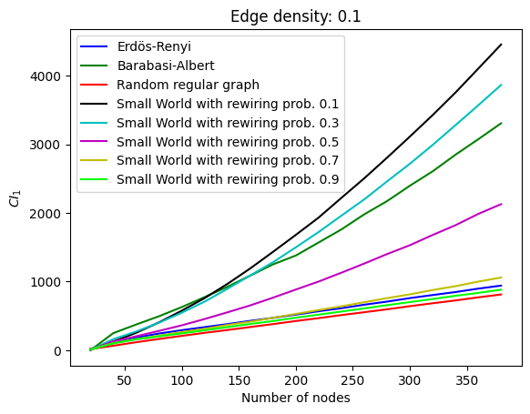
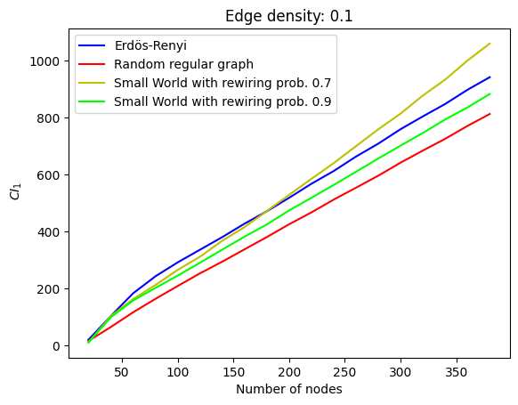
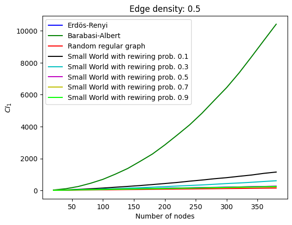
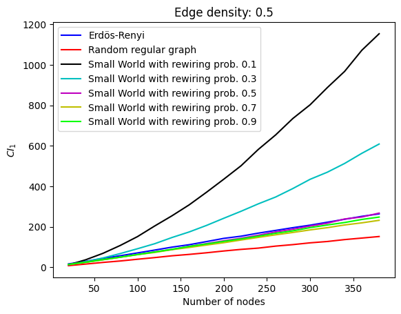
Figure 3: Average $\mathrm{CI}_{1}$ values of the Erdős-Rényi graph, Barabási-Albert graph, random regular graph and Watts-Strogatz graphs with edge densities 0.1 and 0.5.

Our expectation from our theoretical findings was that the growth of $\mathrm{CI}_{1}$ for Erdős-Rényi graphs was linear in $n$, which is verified in our simulation. One would also expect that, as the rewiring probability increases, the Watts-Strogatz graphs exhibit increasingly similar behavior to Erdős-Rényi graphs in terms of clustering, which seems to be the case.

We think that Barabási-Albert model having a large clustering index can be explained as follows: In the resulting graph after many iterations, the degrees of a significant portion of the nodes added to the initial star graph will be very small $(\leq 3)$. When the degree is small, the local clustering coefficient will be 0 or 1 with high probability. Hence, the clustering index can be expected to behave like $Cn^{2}$ asymptotically. This behavior seems to be more easily observed when the edge density increases.

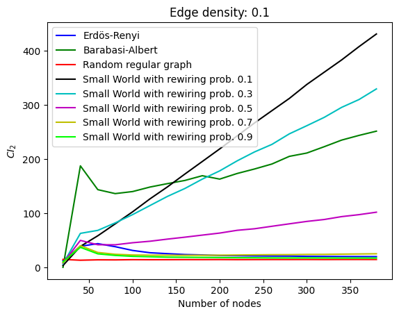
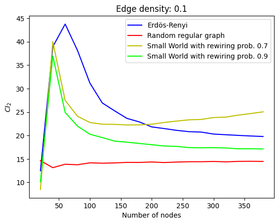
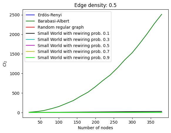
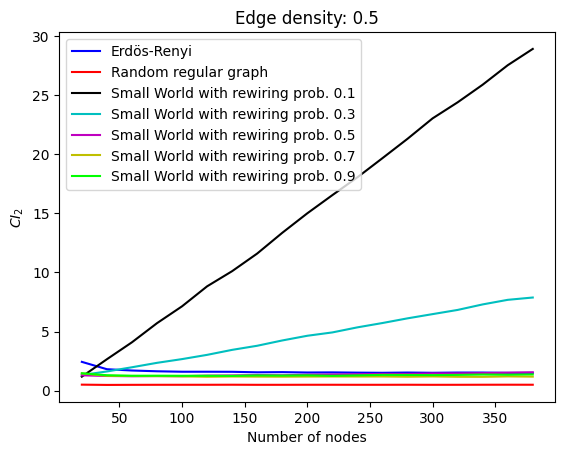
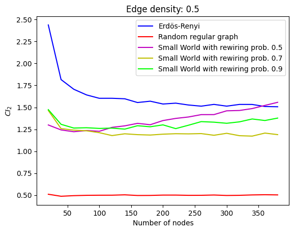
Figure 4: Average $\mathrm{CI}_{2}$ values of the Erdős-Rényi graph, Barabási-Albert graph, random regular graph and Watts-Strogatz graphs with edge densities 0.1 and 0.5.

Next we include the comparison of $\mathrm{CI}_{2}$ for the four models of interest. In the case of Erdős-Rényi, we showed that this index is upper bounded by a constant independent of the number of nodes, and conjectured that it is indeed also lower bounded by a constant. This is indeed the case according to our simulations, where $\mathrm{CI}_{2}$ can be observed to approach $\frac{2(1-p)(1-p^{2})}{p}$ as $n$ increases. Watts-Strogatz graphs with low rewiring probability and Barabási-Albert model again dominate the others in this case. We again observe that as the rewiring probability increases, $\mathrm{CI}_{2}$ of Watts-Strogatz model approaches that of Erdős-Rényi model.

It is also interesting to note that many of our random graphs seem to exhibit a peaking behavior around 40-60 nodes when edge density is 0.1. This behavior is most easily observed when edge density is low, and the position of peaks depend on the edge density; as edge density decreases, the number of nodes corresponding to the peak increases (up to a point). We think that the appearance of these peaks is a result of an equilibrium of two opposing effects:

• As $n$ increases, the number of terms appearing in the sum $\mathrm{CI}_{2}$ also increases.

• As $n$ increases, the variance of the distribution of local clustering coefficients decreases.

When the edge density is 0.5, the Barabási-Albert model again dominates the others; this time by around 2 orders of magnitude at $n=380$. Watts-Strogatz model with lower rewiring probabilities again follow Barabási-Albert graphs in the ranking.

5.3 Results for the degree index

In this subsection we focus on the degree index and compare $\mathrm{DI}_{1}$ and $\mathrm{DI}_{2}$ for the same four random graph models for again varying values of the number of nodes. The first one below is for $\mathrm{DI}_{1}$ and the edge density in $\{0.1,0.5\}$.

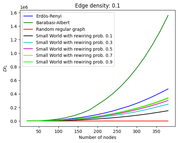
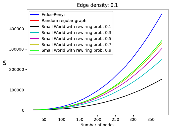
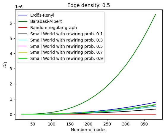
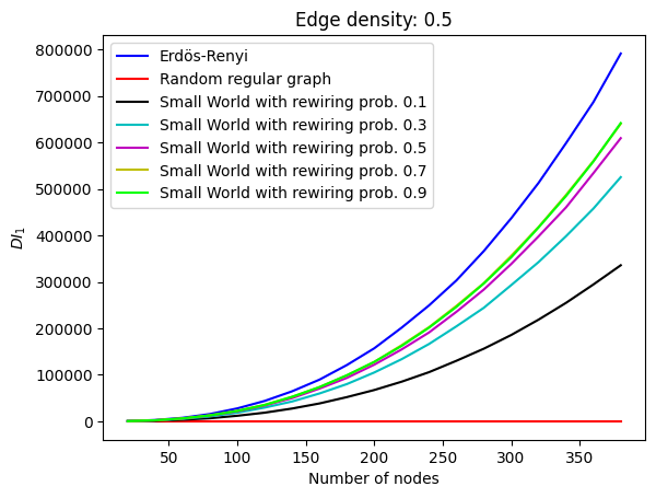
Figure 5: Average $\mathrm{DI}_{1}$ values of the Erdős-Rényi graph, Barabási-Albert graph, random regular graph and Watts-Strogatz graphs with edge densities 0.1 and 0.5.

For either of the edge densities considered, the Barabási-Albert model dominates the other ones significantly. This is not surprising since preferential attachment causes significant number of nodes to have degrees comparable to $n$ and a majority of the nodes to have very small degrees. This causes $\mathbb{E}[|d_{i}-d_{j}|]$ to be of order $n$, which then implies $\mathrm{DI}_{1}=\theta(n^{3})$.

We see that $\mathrm{DI}_{1}$ is zero for the case of random regular graphs, which is already trivial since the degrees in such graphs are the same. We can again observe that small world model behaves similarly to Erdős-Rényi as the rewiring probability increases.

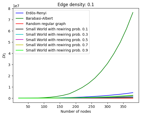
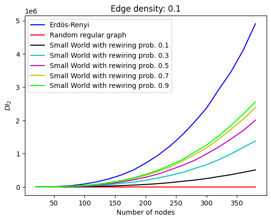
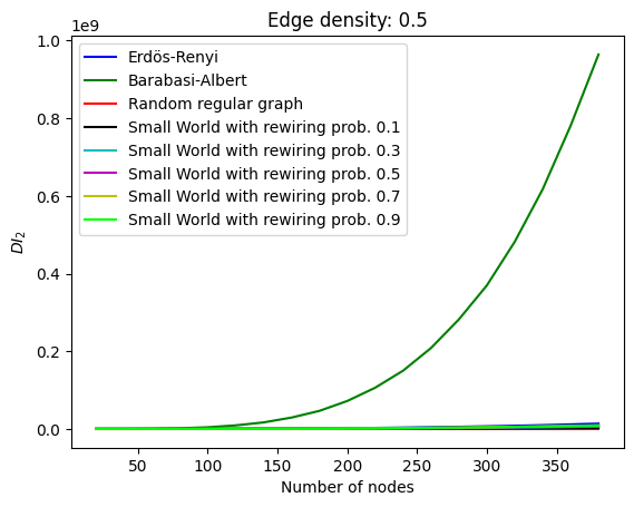
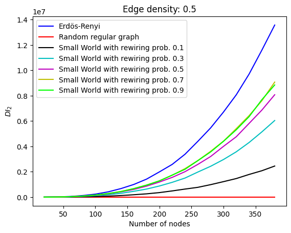
Figure 6: Average $\mathrm{DI}_{2}$ values of the Erdős-Rényi graph, Barabási-Albert graph, random regular graph and Watts-Strogatz graphs with edge densities 0.1 and 0.5.

The above observations for $\mathrm{DI}_{1}$ are also true for $\mathrm{DI}_{2}$, with the modification that $\mathrm{DI}_{1}=\theta(n^{4})$ for Barabási-Albert, as expected. Note also that the $\mathrm{DI}_{2}$ values in our simulations are in agreement with our theoretical results.

6 Conclusion

In this manuscript, besides the well known degree index (or, irregularity), we introduced the concept of clustering index and studied the first moment of both of them in random graphs. Focusing on Erdős-Rényi graphs and the degree case, we were able to obtain either exact or asymptotic expressions for the expected degree indices of interest. Regarding the clustering index case, we obtained a linear upper bound for $\mathbb{E}[\mathrm{CI}_{1}(\mathcal{G})]$, and also showed that $\mathbb{E}[\mathrm{CI}_{2}(\mathcal{G})]$ is bounded above by a constant independent of $n$. Although we had theoretical and simulation based related analysis for random graphs, we have not done a detailed study of the indices of interest for real life complex networks, and we intend to do so in a subsequent work.

One main motivation for studying these indices in our case is their possible use in classification algorithms as features. Characteristics such as average clustering and the average degree are already used in various such problems, and we intend to do an experimental study on the use of degree and clustering indices to see whether they provide improvements in performance in classification problems. A second related path is in the field of finance, more particularly on the detection of financial crises. In a recent work [13], it is argued that a certain graph irregularity measure, namely the Laplace energy, can be used to detect economic crises. We plan to visit this issue with the indices discussed in current paper, and see whether the degree and clustering indices (as certain types of irregularities) can also be considered as a precursor of financial crises.

A last direction we are willing to follow is on computing the exact asymptotics of $\mathrm{CI}_{1}$ and $\mathrm{CI}_{2}$ in case of Erdős-Rényi graphs. For example, focusing on $\mathrm{CI}_{2}$, we were able to obtain a constant upper bound, and simulations suggested that this index indeed like a constant as the number of nodes increases. It would be interesting to verify the validity of this convergence theoretically.

Acknowledgements. Parts of this paper were completed at the Nesin Mathematics Village, the authors would like to thank Nesin Mathematics Village for their kind hospitality. The first author is supported by the BAGEP Award of the Science Academy, Turkey.

References

• [1] Abdo, Hosam, Stephan Brandt, and Darko Dimitrov. “The total irregularity of a graph.” Discrete Mathematics & Theoretical Computer Science 16.Graph Theory (2014).
• [2] Abdo, Hosam, Darko Dimitrov, and Ivan Gutman. “Graphs with maximal $\sigma$ irregularity.” Discrete Applied Mathematics 250 (2018): 57-64.
• [3] Abdo, Hosam, Darko Dimitrov, and Ivan Gutman. “Graph irregularity and its measures.” Applied Mathematics and Computation 357 (2019): 317-324.
• [4] Albert, Réka, and Albert-László Barabási. “Statistical mechanics of complex networks.” Reviews of modern physics 74.1 (2002): 47.
• [5] Albertson, Michael O. “The irregularity of a graph.” Ars Combinatoria 46 (1997): 219-225.
• [6] Chen, Muzi, et al. “Dynamic correlation of market connectivity, risk spillover and abnormal volatility in stock price.” Physica A: Statistical Mechanics and Its Applications 587 (2022): 126506.
• [7] Erdős, P. and Alfréd Rényi. (1959). “On Random Graphs. I” (PDF). Publicationes Mathematicae. 6 (3–4): 290–297.
• [8] Erdős, Paul, and Alfréd Rényi. “On the evolution of random graphs.” Publ. math. inst. hung. acad. sci 5.1 (1960): 17-60.
• [9] Gu, Lei, Hui Lin Huang, and Xiao Dong Zhang. “The clustering coefficient and the diameter of small-world networks.” Acta Mathematica Sinica, English Series 29.1 (2013): 199-208.
• [10] Yin, Hao, Austin R. Benson, and Jure Leskovec. “Higher-order clustering in networks.” Physical Review E 97.5 (2018): 052306.
• [11] Yin, Hao, et al. “Local higher-order graph clustering.” Proceedings of the 23rd ACM SIGKDD international conference on knowledge discovery and data mining. 2017.
• [12] Van Der Hofstad, Remco. Random graphs and complex networks. Cambridge university press, 2024.
• [13] Huang, Chuangxia, et al. ”Can financial crisis be detected? Laplacian energy measure.” The European Journal of Finance 29.9 (2023): 949-976.
• [14] Kantarci, Burcu, and Vincent Labatut. “Classification of complex networks based on topological properties.” 2013 international conference on Cloud and Green Computing. IEEE, 2013.
• [15] Kartun-Giles, Alexander P., and Ginestra Bianconi. “Beyond the clustering coefficient: A topological analysis of node neighbourhoods in complex networks.” Chaos, Solitons & Fractals: X 1 (2019): 100004.
• [16] Soffer, Sara Nadiv, and Alexei Vazquez. “Network clustering coefficient without degree-correlation biases.” Physical Review E 71.5 (2005): 057101.
• [17] Yin, Hao, Austin R. Benson, and Jure Leskovec. “Higher-order clustering in networks.” Physical Review E 97.5 (2018): 052306.
• [18] McDiarmid, Colin. “Concentration.” Probabilistic methods for algorithmic discrete mathematics. Berlin, Heidelberg: Springer Berlin Heidelberg, 1998. 195-248.
• [19] Ross, Nathan. “Fundamentals of Stein’s method.” (2011): 210-293.
• [20] Siew, Cynthia SQ, et al. “Cognitive network science: A review of research on cognition through the lens of network representations, processes, and dynamics.” Complexity 2019.1 (2019): 2108423.
• [21] Silva, Thiago Christiano, and Liang Zhao. Machine learning in complex networks. Springer, 2016.
• [22] West, Douglas Brent. Introduction to graph theory. Vol. 2. Upper Saddle River: Prentice hall, 2001.
• [23] Watts, Duncan J., and Steven H. Strogatz. “Collective dynamics of ‘small-world’networks.” nature 393.6684 (1998): 440-442.
• [24] Li, Yusheng, Yilun Shang, and Yiting Yang. “Clustering coefficients of large networks.” Information Sciences 382 (2017): 350-358.