Abstract. In this paper we discuss the problem of interpolation on straight lines by linear combinations of ridge functions with fixed directions. By using some geometry and/or systems of linear equations, we constructively prove that it is impossible to interpolate arbitrary data on any three or more straight lines by sums of ridge functions with two fixed directions. The general case with more straight lines and more directions is reduced to the problem of existence of certain sets in the union of these lines.

Mathematics Subject Classifications: 15A06, 26B40, 41A05

Keywords: ridge function; interpolation; linear equation; closed path; cycle

1. Introduction

A ridge function is a multivariate function of the format

$$F(\mathbf{x})=g\left(\mathbf{a}\cdot\mathbf{x}\right)=g\left(a_{1}x_{1}+\cdot\cdot\cdot+a_{n}x_{n}\right),$$

where $g:\mathbb{R}\rightarrow\mathbb{R}$ and $\mathbf{a}=\left(a_{1},...,a_{n}\right)$ is a fixed vector (direction) in $\mathbb{R}^{n}\backslash\left\{\mathbf{0}\right\}.$ In other words, a ridge function is a multivariate function constant on the hyperplanes $\mathbf{a}\cdot\mathbf{x}=c$, for any $c\in$ $\mathbb{R}$. These functions arise naturally in various fields. They arise in partial differential equations (where they are called plane waves, see, e.g., [9]), in computerized tomography (see, e.g., [12]), in statistics (especially, in the theory of projection pursuit and projection regression; see, e.g., [5]), in the theory of neural networks (see, e.g., [7]). Finally, these functions are used in modern approximation theory as an effective and convenient tool for approximating and interpolating complicated multivariate functions (see, e.g., [2, 13]). For more on ridge functions and application areas see the monographs by Pinkus [15] and Ismailov [7].

Let $\mathbf{a}^{1},...,\mathbf{a}^{r}$ be fixed pairwise linearly independent directions in $\mathbb{R}^{n}\backslash\left\{\mathbf{0}\right\}$. Consider the following set of linear combinations of ridge functions

$$\mathcal{R}\left(\mathbf{a}^{1},...,\mathbf{a}^{r}\right)=\left\{\sum\limits_{i=1}^{r}g_{i}\left(\mathbf{a}^{i}\cdot\mathbf{x}\right):g_{i}:\mathbb{R}\rightarrow\mathbb{R},i=1,...,r\right\}.$$

Note that the set $\mathcal{R}\left(\mathbf{a}^{1},...,\mathbf{a}^{r}\right)$ is a linear space. We are interested in the problem of interpolation by functions from $\mathcal{R}\left(\mathbf{a}^{1},...,\mathbf{a}^{r}\right)$. Interpolation at a finite number of points by such functions has been considered in Braess, Pinkus [2], Sun [17], Reid, Sun [16], Weinmann [18] and Levesley, Sun [11]. The results therein are complete only in the case of two directions ($r=2$), and three directions in $\mathbb{R}^{2}$.

In [8], Pinkus and Ismailov discussed the problem of interpolation by functions from $\mathcal{R}\left(\mathbf{a}^{1},...,\mathbf{a}^{r}\right)$ in straight lines. To make the problem precise, assume we are given the straight lines $\{t\mathbf{b}^{i}+\mathbf{c}^{i}:t\in\mathbb{R}\}$, $\mathbf{b}^{i}\neq 0,$ $i=1,...,m$. The question they asked is when, for every choice of data $g_{i}(t)$, $i=1,...,m$, there exists a function $G\in\mathcal{R}\left(\mathbf{a}^{1},...,\mathbf{a}^{r}\right)$ satisfying

$$G(t\mathbf{b}^{i}+\mathbf{c}^{i})=g_{i}(t),$$

for all $t\in\mathbb{R}$ and any $i=1,...,m$. The paper [8] totally analyzed this question with one and two directions ($r\leq 2$). It was found necessary and sufficient conditions for the possibility of interpolation on one and two straight lines. One of the major results of [8] dealt with the case of three (or more) distinct straight lines.

Theorem 1.1. (see [8]) Assume we are given linearly independent directions $\mathbf{a}^{1},\mathbf{a}^{2}$ in $\mathbb{R}^{n}$. Then for any three distinct straight lines $\{t\mathbf{b}^{i}+\mathbf{c}^{i}:t\in\mathbb{R}\}$, $i=1,2,3,$ and all $g_{1},g_{2},g_{3}$ defined on $\mathbb{R}$ there does not exist a $G\in\mathcal{R}\left(\mathbf{a}^{1},\mathbf{a}^{2}\right)$ satisfying

$$G(t\mathbf{b}^{i}+\mathbf{c}^{i})=g_{i}(t),~{}t\in\mathbb{R},~{}i=1,2,3.$$

Theorem 1.1 was proved by analyzing certain first order difference equations. In this paper we give a completely different, geometrically explicit and constructive proof for Theorem 1.1.

Our approach will be based on so called paths. A path with respect to the directions $\mathbf{a}^{1}$ and $\mathbf{a}^{2}$ is an ordered set of points $(\mathbf{x}^{1},...,\mathbf{x}^{k})$ in $\mathbb{R}^{n}$ with $\mathbf{x}^{i}\neq\mathbf{x}^{i+1}$ and the units $\mathbf{x}^{i+1}-\mathbf{x}^{i}$ perpendicular alternatively to $\mathbf{a}^{1}$ and $\mathbf{a}^{2}$. That is, after a suitable permutation we have $\mathbf{a}^{1}\cdot$ $\mathbf{x}^{1}=\mathbf{a}^{1}\cdot$ $\mathbf{x}^{2},$ $\mathbf{a}^{2}\cdot$ $\mathbf{x}^{2}=\mathbf{a}^{2}\cdot$ $\mathbf{x}^{3},$ $\mathbf{a}^{1}\cdot$ $\mathbf{x}^{3}=\mathbf{a}^{1}\cdot$ $\mathbf{x}^{4}$, and so on. If $\left(\mathbf{x}^{1},...,\mathbf{x}^{k},\mathbf{x}^{1}\right)$ is a path and $k$ is an even number, then the path $\left(\mathbf{x}^{1},...,\mathbf{x}^{k}\right)$ is said to be a closed path. For example, a set of vertices (ordered clockwise or counterclockwise) of any polygon in $\mathbb{R}^{2}$ with sides parallel to the coordinate axis is a closed path with respect to the coordinate directions $(1,0)$ and $(0,1)$. Fig. 1 describes two different paths in the coordinate plane.

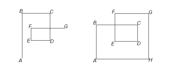
Figure 1: In the first picture, the points $A,B,C,D,E,F,G$, in the given order, form a path with respect to the coordinate directions. The second picture illustrates a closed path.

Paths are geometrically explicit objects. In the special case when $\mathbf{a}_{1}$ and $\mathbf{a}_{2}$ coincide with the coordinate directions these objects were first introduced by Diliberto and Straus [4] (in [4], they are called “permissible lines”). They appeared further in a number of papers with several different names such as “bolts” (see, e.g., [1, 10]), “trips” (see [14]), “links” (see, e.g., [3]). In [6], paths were generalized to those with respect to a finite set of functions. The last objects turned out to be useful in problems of representation by linear superpositions. For a detailed history of paths, their generalizations and various applications see [7].

It should be remarked that the problem of interpolation of arbitrary data on the lines $l_{i}=\{t\mathbf{b}^{i}+\mathbf{c}^{i}:t\in\mathbb{R}\}$, $i=1,...,m,$ by functions from $\mathcal{R}\left(\mathbf{a}^{1},...,\mathbf{a}^{r}\right)$ is equivalent to the problem of the representation of an arbitrarily given $F$ defined on the union $L=\cup_{i=1}^{m}l_{i}$ by such functions (see [8]). Concerning this problem, we have the following result from [6].

Theorem 1.2. Assume we are given two directions $\mathbf{a}^{1}$ and $\mathbf{a}^{2}$ in $\mathbb{R}^{n}$. Let $X$ be any subset of $\mathbb{R}^{n}$. Then every given function defined on $X$ is in $\mathcal{R}\left(\mathbf{a}^{1},\mathbf{a}^{2}\right)$ if and only if there are no finite set of points in $X$ that form a closed path with respect to the directions $\mathbf{a}^{1}$ and $\mathbf{a}^{2}$.

This theorem implies that for solving the interpolation problem on $L$ it is enough to verify whether $L$ contains a closed path. We use this fact in the proof of Theorem 1.1. In other words, we show in the next section that a set of distinct three lines in $\mathbb{R}^{n}$ possesses closed paths with respect to two arbitrarily given directions.

2. The three-line interpolation problem

The following theorem is equivalent to Theorem 1.1.

Theorem 2.1. Assume we are given two linearly independent directions $\mathbf{a}^{1},\mathbf{a}^{2}\in\mathbb{R}^{n}$. Assume, in addition, $l_{i}=\{t\mathbf{b}^{i}+\mathbf{c}^{i}:t\in\mathbb{R}\},$ $i=1,2,3,$ are distinct straight lines in $\mathbb{R}^{n}$ and $L=l_{1}\cup l_{2}\cup l_{3}$. Then there exists a closed path $p=\left(\mathbf{x}^{1},...,\mathbf{x}^{m}\right)$ with respect to the directions $\mathbf{a}^{1}$ and $\mathbf{a}^{2}$ such that $p\subset L$.

Proof. Complete the pair $\{\mathbf{a}^{1},\mathbf{a}^{2}\}$ to a basis $\{\mathbf{a}^{1},\mathbf{a}^{2},...,\mathbf{a}^{n}\}$ in $\mathbb{R}^{n}$. The nonsingular linear transformation of coordinates $S:\mathbf{x}=(x_{1},...,x_{n})\rightarrow\mathbf{y}=(y_{1},...,y_{n}),$ $y_{i}=\mathbf{a}^{i}\cdot$ $\mathbf{x},$ $i=1,...,n$, has the property $\mathbf{e}^{i}\cdot$ $\mathbf{y}=\mathbf{a}^{i}\cdot$ $\mathbf{x}$, where $\mathbf{e}^{i}$ is the $i$-th unit vector (that is, the vector having $1$ in the $i$-th position and zeros everywhere else). Therefore, if $\left(\mathbf{x}^{1},...,\mathbf{x}^{m}\right)$ is a path with respect to $\mathbf{a}^{1},\mathbf{a}^{2}$, then the transformed set $\left(\mathbf{y}^{1},...,\mathbf{y}^{m}\right)$ will be a path with respect to $\mathbf{e}^{1},\mathbf{e}^{2}$. This fact admits to choose $\mathbf{a}^{1}=\mathbf{e}^{1}=(1,0,...,0)$ and $\mathbf{a}^{2}=\mathbf{e}^{2}=(0,1,...,0)$. Thus we will prove the theorem if we prove it for the basis directions $\mathbf{e}^{1}$ and $\mathbf{e}^{2}$.

Let $P$ be the orthogonal projection of $\mathbb{R}^{n}$ onto the plane generated by the vectors $\mathbf{e}^{1}$ and $\mathbf{e}^{2}$, that is, onto the $x_{1}x_{2}$ plane. Clearly, the image of a straight line under this projection will be a straight line or a point. Note that if for some $l_{i}$ the image of it is a point, then any two distinct points $\mathbf{x}^{1},\mathbf{x}^{2}\in l_{i}$ form a closed path, since in this case $\mathbf{x}^{2}-\mathbf{x}^{1}$ is orthogonal to both $\mathbf{e}^{1}$ and $\mathbf{e}^{2}$. Further note that the projections of two (or all three) of $l_{i}$ may coincide. In this case we also have a closed path $(\mathbf{x}^{1},\mathbf{x}^{2})$ with the vertices $\mathbf{x}^{1}$ and $\mathbf{x}^{2}$ lying in different straight lines. We see that it is enough to consider the general case when the images of all the lines $l_{i}$ are again straight lines and these images do not coincide. If we prove that the image $PL=Pl_{1}\cup Pl_{2}\cup Pl_{3}\subset\mathbb{R}^{2}$ contains a closed path $\left(\mathbf{x}^{1},...,\mathbf{x}^{2m}\right)$ with respect to the vectors $(1,0)$ and $(0,1)$, then the initial set $L$ contains a closed path with respect to $\mathbf{e}^{1}$ and $\mathbf{e}^{2}$. Indeed, if for some $\mathbf{x}^{i}$, $i=1,...,2m$, the preimage $P^{-1}\mathbf{x}^{i}\cap L$ has more than a single point, then any two of them form a closed path. And if $\left(\mathbf{x}^{1},...,\mathbf{x}^{2m}\right)$ is a closed path in $PL$ and for each $\mathbf{x}^{i}$, the preimage $P^{-1}\mathbf{x}^{i}\cap L$ is a single point, denoted here by $\mathbf{z}^{i}$, then $\left(\mathbf{z}^{1},...,\mathbf{z}^{2m}\right)$ is a closed path in $L.$ This observation reduces the problem to the two-dimensional case and we will prove the theorem if we prove that the union of any distinct three lines in $\mathbb{R}^{2}$ contain a closed path with respect to the coordinate directions.

Concerning three lines in $\mathbb{R}^{2}$ we have only the following options.

Case 1. At least one of $l_{i}$ is parallel to the $x_{1}$ or $x_{2}$ axis. In this case it is not difficult to see that there exist four-point closed paths.

Case 2. The straight lines $l_{i}=\{t\mathbf{b}^{i}+\mathbf{c}^{i}:t\in\mathbb{R}\},$ $i=1,2,3,$ are parallel. That is, $\mathbf{b}^{1}=\mathbf{b}^{2}=\mathbf{b}^{3}.$ Let $\mathbf{b}^{i}=\mathbf{b}=(b_{1},b_{2})$, $\mathbf{c}^{i}=(c_{1}^{i},c_{2}^{i}),$ $i=1,2,3$.

Linear algebraic approach. Consider a six-point set $(\mathbf{x}^{1},\mathbf{x}^{2},\mathbf{x}^{3},\mathbf{x}^{4},\mathbf{x}^{5},\mathbf{x}^{6})$ in $l_{1}\cup l_{2}\cup l_{3}$ with the property that $\mathbf{x}^{1},\mathbf{x}^{4}\in l_{1},$ $\mathbf{x}^{2},\mathbf{x}^{5}\in l_{2},$ and $\mathbf{x}^{3},\mathbf{x}^{6}\in l_{3}$. Put $\mathbf{x}^{k}=t_{k}\mathbf{b}+\mathbf{c}^{k},$ $k=1,...,6$, $\mathbf{c}^{j+3}=\mathbf{c}^{j}$, $j=1,2,3.$ Let us check if these points could form a closed path in the given order. This is possible if the system of linear equations

$$\left\{\begin{array}[]{c}t_{1}b_{1}+c_{1}^{1}=t_{2}b_{1}+c_{1}^{2}\\ t_{2}b_{2}+c_{2}^{2}=t_{3}b_{2}+c_{2}^{3}\\ t_{3}b_{1}+c_{1}^{3}=t_{4}b_{1}+c_{1}^{1}\\ t_{4}b_{2}+c_{2}^{1}=t_{5}b_{2}+c_{2}^{2}\\ t_{5}b_{1}+c_{1}^{2}=t_{6}b_{1}+c_{1}^{3}\\ t_{6}b_{2}+c_{2}^{3}=t_{1}b_{2}+c_{2}^{1}\end{array}\right.$$

has a solution. In fact, applying Cramer’s rule, one can see that this system has infinitely many solutions $(t_{1},t_{2},...,t_{6})$. This means that we have infinitely many six-point closed paths with vertices positioned at these lines. Note that if $(t_{1},t_{2},...,t_{6})$ is a solution of the system (2.1), then $(t_{1}+\alpha,t_{2}+\alpha,...,t_{6}+\alpha)$ is also a solution for any $\alpha\in\mathbb{R}$. Thus, we see that all six-point closed paths satisfying (2.1) can be obtained by a single six-point closed path by the translation $T(\mathbf{x})=\mathbf{x}+\alpha\mathbf{b}$.

Geometric approach. There is also a geometric approach to this case. Consider a path $(A,B,C,D,E,F,A^{\prime})$ such that $A,D,A^{\prime}\in l_{1}$, $B,E\in l_{2}$, $C,F\in l_{3}$. That is, the vertices of this path lie alternatively at the lines $l_{1},l_{2},l_{3}$. It is not difficult to see that $\overrightarrow{AB}+\overrightarrow{CD}+\overrightarrow{EF}=\overrightarrow{\mathbf{0}}$ and $\overrightarrow{BC}+\overrightarrow{DE}+\overrightarrow{FA^{\prime}}=\overrightarrow{\mathbf{0}}$. Hence $\overrightarrow{AA^{\prime}}=\overrightarrow{\mathbf{0}}$ which yields $A=A^{\prime}$. Thus the path $(A,B,C,D,E,F)$ is closed. See Fig. 2 for the geometric illustration of this case.

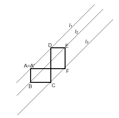
Figure 2: The six-point closed path $(A,B,C,D,E,F)$ in $l_{1}\cup l_{2}\cup l_{3}$.

Case 3. The lines $l_{i}$ have a common point of intersection $(\xi_{1},\xi_{2})$ and none of them is parallel to $x_{1}$ or $x_{2}$ axis. By translation we can make that $(\xi_{1},\xi_{2})=(0,0)$. So without loss of generality we may assume that the lines intersect at the coordinate origin. Let $x_{2}=px_{1}$, $x_{2}=qx_{1}$, $x_{2}=rx_{1}$ be equations of these three lines. Then it is easy to verify that the set

$$\{(p,pq),(p,pr),(r,pr),(r,qr),(q,qr),(q,pq)\}$$

is a closed path in $l_{1}\cup l_{2}\cup l_{3}$.

Case 4. The lines do not intersect at the same point, they are not parallel and none of them is parallel to the coordinate axis. We claim that in this case there is a four-point closed path $\left\{(u_{1},u_{2}),(u_{1},v_{2}),(v_{1},v_{2}),(v_{1},u_{2})\right\}$ in the union $L$ of these lines. Let us prove this. Assume $x_{2}=ax_{1}+b,$ $x_{2}=cx_{1}+d,$ $x_{2}=ex_{1}+f$ are the equations of $l_{1},l_{2},l_{3}$, respectively.

Linear algebraic approach. We seek such a closed path with the vertices $(u_{1},u_{2}),(v_{1},v_{2})$ in one line and with $(u_{1},v_{2}),(v_{1},u_{2})$ each in other two lines, respectively. If $(u_{1},u_{2}),(v_{1},v_{2})\in l_{1}$, $(u_{1},v_{2})\in l_{2}$, $(v_{1},u_{2})\in l_{3}$, then we have the system of linear equations

$$\left\{\begin{array}[]{c}-au_{1}+u_{2}=b\\ -av_{1}+v_{2}=b\\ -cu_{1}+v_{2}=d\\ -ev_{1}+u_{2}=f\end{array}\right..$$

The determinant of this system (up to a sign) is equal to $ce-a^{2}$. In other two cases when $(u_{1},u_{2}),(v_{1},v_{2})\in l_{2}$, $(u_{1},v_{2})\in l_{1}$, $(v_{1},u_{2})\in l_{3}$ and when $(u_{1},u_{2}),(v_{1},v_{2})\in l_{3}$, $(u_{1},v_{2})\in l_{1}$, $(v_{1},u_{2})\in l_{2}$, the determinants of the corresponding systems will be $ae-c^{2}$ and $ac-e^{2}$, respectively. If the expressions $ce-a^{2}$, $ae-c^{2}$ and $ac-e^{2}$ are all zero, then $a=c=e$ and hence the lines are parallel. This reduces the problem to Case 2. If one of these expressions is not zero, then the corresponding system has a unique solution $u_{1},u_{2},v_{1},v_{2}$. Note that $u_{1}=v_{1}$ or $u_{2}=v_{2}$ is possible if and only if the lines intersect at the same point, which reduces the problem to Case 3 above. Thus we obtain that there exists a four-point closed path in the union of the given three straight lines. Certainly, the vertices of this path can be explicitly determined by the coefficients $a,b,c,d,e,f$.

Geometric approach. Let $\Omega$ be the set of all non-degenerate rectangles with sides parallel to the coordinate axis. Let $l_{1}$ and $l_{2}$ intersect at a point $O$ forming four rays $r_{1},r_{2},r_{3},r_{4}$ with a vertex at $O$. If $r$ is any of these rays and $l_{i}$ is the line not containing $r$, then for any $P\in r\backslash\{O\}$, we let $\Pi_{P}\in\Omega$ be the rectangle with one vertex at $P$ and two adjacent (to $P$) vertices at $l_{i}$. We will denote the fourth vertex of this rectangle by $v(P)$. Then the set $\{v(P):P\in r\backslash\{O\}\}\cup\{O\}$ is a ray at the vertex $O$; If $r=r_{i}$, then we denote this ray by $s_{i}$. The rays $s_{1},s_{2},s_{3},s_{4}$ are all distinct; hence at least one of them intersects $l_{3}$. This intersection point $v(P)\in l_{3}$ and the three points considered above form a four-closed path in $l_{1}\cup l_{2}\cup l_{3}$. See Fig. 3 for the geometric illustration of this case.

Figure 3: Four-point closed path in $l_{1}\cup l_{2}\cup l_{3}$. The vertex $v(P)$ depends on $P$. There exists $P\in l_{1}\cup l_{2}$ such that $v(P)\in l_{3}$.

Theorem 2.1 has been proven.

Remark. One and two straight lines in $\mathbb{R}^{n}$ may not contain closed paths, hence making the ridge function interpolation possible. The characterization of such straight lines was given in [8].

3. The case of three or more directions

Let us consider the interpolation problem in the case when we have three or more directions. Given $m$ straight lines $l_{1},...,l_{m}$ in $\mathbb{R}^{n}$, can we interpolate arbitrary data on these lines by functions from $\mathcal{R}\left(\mathbf{a}^{1},...,\mathbf{a}^{r}\right)$, $r\geq 3$? In [8], it was conjectured that it should be possible, except in certain specific cases, to interpolate along $m$ straight lines, if $m\leq r$. And it should be impossible to interpolate arbitrary data on any $m$ straight lines, if $m>r$. Although, we do not know a solution to this general problem of interpolation, we want as in the previous sections to reduce it to the more tractable problem. The latter will involve cycles – mathematical objects which are generalizations of closed paths (see [7, Chapter 1]). Let $\delta_{A}$ denote the characteristic function of a set $\ A\subset\mathbb{R}.$ That is,

$$\delta_{A}(y)=\left\{\begin{array}[]{c}1,~{}if~{}y\in A\\ 0,~{}if~{}y\notin A.\end{array}\right.$$

A set of points $\{\mathbf{x}^{1},\ldots,\mathbf{x}^{k}\}\subset\mathbb{R}^{n}$ is called a cycle with respect to the directions $\mathbf{a}^{1},...,\mathbf{a}^{r}$ if there exists a vector $\lambda=(\lambda_{1},\ldots,\lambda_{k})$ with the nonzero components such that for any $i=1,\ldots,r$

$$\sum_{j=1}^{k}\lambda_{j}\delta_{\mathbf{a}^{i}\cdot\mathbf{x}^{j}}(t)=0,$$

for all $t\in\mathbb{R}$.

Let us explain Eq. (3.1) in detail. We will see that, in fact, it stands for a system of linear equations. Fix the subscript $i.$ Let the set $\{\mathbf{a}^{i}\cdot\mathbf{x}^{j},$ $j=1,...,k\}$ have $s_{i}$ different values, which we denote by $\gamma_{1}^{i},\gamma_{2}^{i},...,\gamma_{s_{i}}^{i}.$ Take the first number $\gamma_{1}^{i}.$ Putting $t=\gamma_{1}^{i}$, we obtain from (3.1) that

$$\sum_{j}\lambda_{j}=0,$$

where the sum is taken over all $j$ such that $\mathbf{a}^{i}\cdot\mathbf{x}^{j}=\gamma_{1}^{i}.$ This is the first linear equation in $\lambda_{j}$ corresponding to $\gamma_{1}^{i}$. Take now $\gamma_{2}^{i}$. By the same way, putting $t=\gamma_{2}^{i}$ in (3.1), we can form the second equation. Continuing until $\gamma_{s_{i}}^{i}$, we obtain $s_{i}$ linear homogeneous equations in $\lambda_{1},...,\lambda_{k}$. The coefficients of these equations are the integers $0$ and $1$. By varying $i$, we finally obtain $s=\sum_{i=1}^{r}s_{i}$ such equations. Hence (3.1), in its expanded form, stands for the system of these linear equations. Thus $\{\mathbf{x}^{1},\ldots,\mathbf{x}^{k}\}$ is a cycle if the system of linear equations of the form (3.1) has a solution with nonzero components.

For example, assume $r=2,$ $\mathbf{a}^{1}\cdot\mathbf{x}^{1}=\mathbf{a}^{1}\cdot\mathbf{x}^{2}$, $\mathbf{a}^{2}\cdot\mathbf{x}^{2}=\mathbf{a}^{2}\cdot\mathbf{x}^{3}$, $\mathbf{a}^{1}\cdot\mathbf{x}^{3}=\mathbf{a}^{1}\cdot\mathbf{x}^{4}$,…, $\mathbf{a}^{2}\cdot\mathbf{x}^{k-1}=\mathbf{a}^{2}\cdot\mathbf{x}^{k}$,$\mathbf{a}^{1}\cdot\mathbf{x}^{k}=\mathbf{a}^{1}\cdot\mathbf{x}^{1}$ Then it is not difficult to see that for a vector $\lambda=(\lambda_{1},\ldots,\lambda_{k})$ with the components $\lambda_{i}=(-1)^{i},$ we have

$$\sum_{j=1}^{k}\lambda_{j}\delta_{\mathbf{a}^{i}\cdot\mathbf{x}^{j}}=0,$$

for $i=1,2.$ Thus, the set $p=\{\mathbf{x}^{1},\ldots,\mathbf{x}^{k}\}$ is a cycle with respect to the directions $\mathbf{a}^{1}$ and $\mathbf{a}^{2}$. Note that $p$ is also a closed path (after some suitable permutation of its points which we assume to be as given). Hence any closed path is a cycle. It is not difficult to see that any cycle with respect to two directions is a union of closed paths with respect to the same directions.

Another example is the set $\{(0,0,0),~{}(0,0,1),~{}(0,1,0),~{}(1,0,0),~{}(1,1,1)\}$ in $\mathbb{R}^{3}$, which forms a cycle with respect to the coordinate directions. In this example, the vector $\lambda$ above can be taken as $(-2,1,1,1,-1).$

In [6], the second author, in particular, proved that any function $F$ defined on a given $X\subset\mathbb{R}^{n}$ belongs to $\mathcal{R}\left(\mathbf{a}^{1},...,\mathbf{a}^{r}\right)$ if and only if $X$ does not contain cycles with respect to $\mathbf{a}^{1},...,\mathbf{a}^{r}$. Thus the interpolation problem on $m$ straight lines can be reduced to the problem of existence of cycles in these lines. In fact, the interpolation problem is solvable if and only if the union of these lines does not contain cycles. Paralleling Theorem 2.1 above, we speculate that any given $m$ distinct straight lines in $\mathbb{R}^{n}$ contain a cycle with respect to $r$ directions if and only if $r<m$. This is an equivalent formulation of the above conjecture.

Acknowledgments. The second author is grateful to Namig Guliyev for inspiring discussions and his input to the analysis of Case 4 above.

References

[1] V. I. Arnold, On functions of three variables (Russian) Dokl. Akad. Nauk SSSR114 (1957), 679-681; English transl. in Amer. Math. Soc. Transl. 28 (1963), 51-54.
[2] D. Braess, A. Pinkus, Interpolation by ridge functions, J. Approx. Theory73 (1993), 218-236.
[3] R. C. Cowsik, A. Klopotowski, M. G. Nadkarni, When is ?, Proc. Indian Acad. Sci. Math. Sci.109
(1999), 57–64.
[4] S. P. Diliberto, E. G. Straus, On the approximation of a
function of several variables by the sum of functions of fewer variables,
Pacific J. Math.1 (1951), 195-210.
[5] J. H. Friedman and W. Stuetzle, Projection pursuit regression,
J. Amer. Statist. Assoc.76 (1981), 817-823.
[6] V. E. Ismailov, On the representation by linear
superpositions, J. Approx. Theory151 (2008), 113-125.
[7] V. E. Ismailov, Ridge functions and applications in
neural networks, Mathematical Surveys and Monographs 263, American
Mathematical Society, 186 pp.
[8] V. E. Ismailov, A. Pinkus, Interpolation on lines by ridge
functions, J. Approx. Theory175 (2013), 91-113.
[9] F. John, Plane Waves and Spherical Means Applied to
Partial Differential Equations, Interscience, New York, 1955.
[10] S. Ya. Khavinson, Best approximation by linear
superpositions (approximate nomography), Translated from the Russian
manuscript by D. Khavinson. Translations of Mathematical Monographs, 159.
American Mathematical Society, Providence, RI, 1997, 175 pp.
[11] J. Levesley, X. Sun, Scattered Hermite interpolation by ridge
functions, Numer. Funct. Anal. Optim.16 (1995), 989-1001.
[12] B. F. Logan, L. A. Shepp, Optimal reconstruction of a function
from its projections, Duke Math.J.42 (1975), 645-659.
[13] V. E. Maiorov, On best approximation by ridge functions,
J. Approx. Theory99 (1999), 68-94.
[14] D. E. Marshall, A. G. O’Farrell, Uniform approximation by
real functions, Fund. Math.104 (1979), 203-211.
[15] A. Pinkus, Ridge Functions, Cambridge Tracts in
Mathematics, 205. Cambridge University Press, Cambridge, 2015, 218 pp.
[16] L. Reid, X. Sun, Distance matrices and ridge function
interpolation, Canad. J. Math.45 (1993), 1313-1323.
[17] X. Sun, Ridge function spaces and their interpolation
property, J. Math. Anal. Appl.179 (1993), 28-40.
[18] A.Weinmann, The interpolation problem for ridge functions,
Numer. Funct. Anal. Optim.15 (1994), 183-186.