Robust chaos in a totally symmetric network of four phase oscillators

Abstract

We provide conditions on the coupling function such that a system of 4 globally coupled identical oscillators has chaotic attractors, a pair of Lorenz attractors or a 4-winged analogue of the Lorenz attractor. The attractors emerge near the triple instability threshold of the splay-phase synchronization state of the oscillators. We provide theoretical arguments and verify numerically, based on the pseudohyperbolicity test, that the chaotic dynamics are robust with respect to small, e.g. time-dependent, perturbations of the system. The robust chaoticity should also be inherited by any network of weakly interacting systems with such attractors.

Introduction.

The study of emergent behavior in networks of coupled oscillators is an important problem with application to various fields of science and engineering, including neuroscience [1, 2, 3], molecular and cellular biology [4, 5], medical engineering [6, 7], chemistry and material science [8, 9, 10, 11], optics [12, 13, 14], solid state physics [15, 16, 17], mechanics [18, 19, 20], etc.

The idea that a diffusive coupling in a system of identical damped oscillators can create instabilities leading to the symmetry breaking and the pattern formation can be traced back to Turing [21]. The emergence of non-trivial, even chaotic, dynamics in such systems at an intermediate coupling strength is now a well-established fact [22, 23, 24]. Without the damping (i.e., when the individual systems in the network have an asymptotically stable periodic orbit), non-trivial patterns of collective behavior of the oscillators phases are formed at an arbitrarily weak coupling [25, 26] (the strong coupling leads to synchronization [27, 28, 29, 30]).

The dynamics of a totally symmetric network of weakly coupled identical oscillators are modelled by the generalized Kuramoto model [28, 25, 26]

$$\dot{\phi}_{j}=\omega+\frac{1}{N}\,\sum_{i=1}^{N}g(\phi_{i}-\phi_{j}),\ \ j=1,\ldots,N,$$ (1)

where $\phi_{j}\in S^{1}$ is the phase of the $j$-th oscillator, $N$ is the number of the oscillators, $\omega$ is the common frequency, and the $2\pi$-periodic function $g(\phi)$ describes the coupling.

In the classical Kuramoto-Sakaguchi model [28, 31], one puts $g(\phi)=A\sin(\phi+\xi)$. This is an important special case, describing the interaction of small amplitude oscillations, e.g. when the parameters of an individual oscillator are close to the Andronov-Hopf bifurcation at which the small-amplitude stable periodic regime was created, cf. [32]. For such single-harmonic function $g$, regardless of the number of oscillators, the dynamics are either completely integrable (quasiperiodic, when $g(\phi)=A\cos(\phi)$ [33]) or converge to a synchronized state [34, 35].

However, when the oscillators are far from the Andronov-Hopf bifurcation and the oscillations’ amplitude is not small, the coupling function $g$ can be arbitrary. This strongly influences the network dynamics. Thus, for $N\geq 4$, adding the second Fourier harmonic to $g(\phi)$ can lead to apparently chaotic dynamics [36, 37, 38, 39].

Note that the previously observed chaotic attractors in the homogeneous network of oscillators (1) are not robust with respect to a variation of parameters. This is clearly demonstrated by the Lyapunov diagrams in Refs. [37, 40, 39], where parameter values corresponding to chaos (the positive top Lyapunov exponent) alternate with those corresponding to trivial attractors. Such non-robustness is a quite common feature of chaotic dynamics in general and is often observed in models of various nature [41, 42]. The existence of the multitude of stability windows in the parameter space makes it impossible to be certain whether a regime observed in a numerical experiment is indeed chaotic, or it is just a long transient which could eventually degenerate into a regular regime such as a stable periodic orbit or a stable stationary state.

In this Letter, we show that system (1) with $N=4$ oscillators can demonstrate, in certain regions of parameter values, a robust chaotic behavior, with no stability windows. We give a rigorous proof of the existence of these regions and provide explicit conditions on the coupling function $g(\phi)$ which allow one to find them, see conditions (4), (Triple instability and robust chaos.). We apply the theoretical results to an example of the coupling function with 4 Fourier modes: $g(\phi)=\sum_{k=1}^{4}A_{k}\sin(k\,\phi+\xi_{k})$, for which we determine the regions of robust and non-robust chaos numerically (we also show that the presence of the 4th harmonic is necessary for the robust chaos to appear).

The robust chaotic attractors we find are 4-winged analogues of the classical Lorenz attractor, see Refs. [43, 44]. Importantly, the robustness of chaos means here more than mere stability with respect to small variations of parameters. These attractors remain chaotic under time-dependent perturbations (periodic, quasiperiodic), and any network of weakly coupled, identical systems with attractors of this type is also robustly chaotic.

Pseudohyperbolicity.

To establish the robustness of chaos, we use the notion of pseudohyperbolicity introduced in [45]. It is based on the computation of Lyapunov exponents and the verification of the continuity of certain fields of invariant Lyapunov subspaces [46, 47, 48] at points of the attractor.

Given an orbit in a chaotic attractor, one computes its Lyapunov exponents $\lambda_{1},\dots,\lambda_{N}$ (indexed in the decreasing order). Let $\lambda_{1}\geq\dots\geq\lambda_{p}\;>\;\lambda_{p+1}\geq\dots\geq\lambda_{N}$ for some $p$. Then, at each point of the orbit there are linear subspaces $E_{1}$ and $E_{2}$ (${\rm dim}(E_{1})=p$, ${\rm dim}(E_{2})=N-p$) such that the field of these subspaces is invariant with respect to the linearization of the system along the trajectory. For the linearized system, the exponential growth (or contraction) rate for the vectors in $E_{1}$ is bounded from below by $\lambda_{p}$ and it is bounded from above by $\lambda_{p+1}$ for the vectors in $E_{2}$. The foundational Oseledets theorem [49] guarantees the existence of Lyapunov exponents and the corresponding invariant subspaces $E_{1,2}$ for a representative orbit in the attractor, but it does not distinguish between the following two possibilities: the fields of subspaces $E_{1,2}$ either admit an extension by continuity to the closure of the orbit, or not. The general theory only gives a measurable dependence of $E_{1,2}$ on the point in the attractor, and not continuous a priori.

When the dependence is continuous, the angle between $E_{1}$ and $E_{2}$ stays bounded away from zero and this splitting into a direct sum of two invariant subspaces persists at all small perturbations [50]. In this case, the attractor is called pseudohyperbolic if $\lambda_{1}+\dots+\lambda_{p}>0$, i.e., the total volume is expanded in $E_{1}$. This property also survives small perturbations. Since the volume expansion in an invariant subspace automatically guarantees the positivity of the top Lyapunov exponent for every orbit in the attractor, the pseudohyperbolicity implies the robustness of chaotic dynamics [51].

All known examples of robustly chaotic attractors are pseudohyperbolic. This includes hyperbolic and partially-hyperbolic attractors [52, 53, 54], Lorenz-like attractors [55, 56, 57, 58, 59], and others [45, 42, 60, 61, 62, 63], as well as their discretized versions and time-periodic perturbations [64, 51]. On the other hand, the theory of homoclinic tangencies suggests that stability windows can emerge easily when chaotic attractors without a pseudohyperbolic structure are perturbed [65, 41, 66]. Therefore, we proposed in Ref. [42] the pseudohyperbolicity as a universal criterion for the robust chaoticity.

Numerics.

The robustness allows one to be sure that a numerically produced “strange attractor” corresponds indeed to a truly chaotic regime and is not a transient or an effect of the inevitable noise. The pseudohyperbolicity criterion makes the numerical verification of the robustness quite straightforward. First, one computes the Lyapunov exponents, chooses $p$ such that $\lambda_{p}>\lambda_{p+1}$ and $\lambda_{1}+\dots+\lambda_{p}>0$ (the volume expansion in $E_{1}$). Then, the rest is to check the continuous dependence of the corresponding subspaces $E_{1,2}$ on a point in the attractor. The continuity can be verified directly [42], or by evaluating the angles between $E_{1}$ and $E_{2}$ and checking that they are bounded away from zero [67, 68, 69].

We applied this strategy to system (1) with

$$g(\phi)=A_{1}\sin(\phi+\xi_{1})+\sin(2\phi+\xi_{2})+A_{4}\sin(4\phi).$$ (2)

By the phase-shift symmetry, it is natural to introduce phase differences $\theta_{j}=\phi_{j}-\phi_{4}$ (we let $\theta_{4}=0$ for the convenience of notation). System (1) becomes 3-dimensional:

$$\dot{\theta}_{j}=\frac{1}{4}\,\sum_{i=1}^{4}\bigl{[}g(\theta_{i}-\theta_{j})-g(\theta_{i})\bigr{]},\ \ j=1,2,3.$$ (3)

We put $A_{1}=-1$, $\xi_{1}=-0.01$ and did the following experiment: at each value of the parameters $(\xi_{2},A_{4})\in[1.62,..,1.92]\times[-0.1,...,0.013]$ from the grid of $1000\times 1000$ points, we took the orbit with the initial condition $(\theta_{1},\theta_{2},\theta_{3})=(1,1.5,3)$ and consider the segment of this orbit with $t\in[10^{4},10^{5}]$ as an approximation of the attractor of system (3). We computed the Lyapunov exponents $\lambda_{1}\geq\lambda_{2}\geq\lambda_{3}$, and marked the attractor as chaotic if $\lambda_{1}\geq 0.005>0$ (blue points in Fig. 1). We consider the attractor robustly chaotic (orange in Fig. 1), if the orbit passes the pseudohyperbolicity test. For that, we checked whether $\lambda_{1}+\lambda_{2}\geq 0.005$, $\lambda_{2}>\lambda_{3}$, and the angle between the corresponding two-dimensional volume-expanding Lyapunov subspace $E_{1}$ and one-dimensional contracting Lyapunov subspace $E_{2}$ is bounded away from zero: $\alpha\geq 0.005$ at each point of the numerically generated attractor.

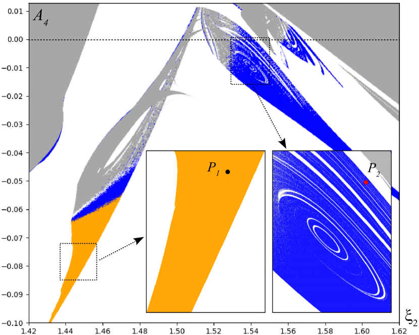
Figure 1: Lyapunov diagram for system (3) in the parameter plane $(\xi_{2},A_{4})$ for $\xi_{1}=-0.01,A_{1}=-1$. At each parameter value from the grid $1000\times 1000$, we compute the Lyapunov exponents $\lambda_{1}\geq\lambda_{2}\geq\lambda_{3}$. If $\lambda_{1}>0$, we additionally check that $\lambda_{1}+\lambda_{2}>0$, $\lambda_{2}>\lambda_{3}$, and the minimal angle $\alpha$ between the Lyapunov subspaces $E_{1}$ and $E_{2}$ is bounded away from zero. In the orange region these conditions are fulfilled, i.e., we have a robust chaotic attractor. In the blue region, $\alpha\approx 0$, so the pseudohyperbolicity conditions are violated, and the chaos is not robust; one can see numerous stability windows in the blue region. In the white and gray regions, the attractor is a periodic orbit or a stationary state, respectively.

The resulting diagram is shown in Fig. 1. In the orange region, the pseudohyperbolicity conditions are satisfied. There are no stability windows, as is clearly visible in the left inset. In the blue regions, we have both the area-expansion $\lambda_{1}+\lambda_{2}>0$ and dominated splitting conditions $\lambda_{2}>\lambda_{3}$, but the angle $\alpha$ is not separated from zero. Therefore, chaotic attractors in these regions are not pseudohyperbolic. This is in agreement with the presence of stability windows (white color – stable periodic orbits; gray – a stable stationary state) inside the regions of chaoticity, see the right inset in Fig. 1.

The chaotic attractors from the orange and blue regions (at points $P_{1}$ and $P_{2}$, respectively) are shown in Fig. 2. Note that they have quite similar shape, but the attractor in Fig. 2a is robustly chaotic, whereas the attractor in Fig. 2b fails the pseudohyperbolicity test. Hence, one cannot reliably conclude whether this is a genuine chaos or a chaotic transient sustained by the numerical noise.

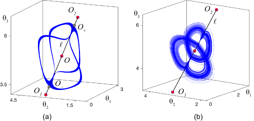
Figure 2: (a) Pseudohyperbolic attractor at $(\xi_{2},A_{4})=(1.45,-0.074)$ (the point $P_{1}$ taken in the orange region in Fig. 1); (b) non-pseudohyperbolic attractor at $(\xi_{2},A_{4})=(1.545,-0.003)$ (the point $P_{2}$ taken in the blue region in Fig. 1). At Fig. b, the invariant line $l$ contains three equilibria: stable equilibria $O_{1,2}$ and the equilibrium $O$, which is unstable in $l$ and is stable in a transverse direction. At Fig. a, the equilibria $O_{1,2}$ are unstable in $l$, and the invariant line contain two additional equilibria $O_{\pm}$, which are stable in $l$ and unstable in a transverse direction.

Note that the line $A_{4}=0$ (that corresponds to the only first 2 harmonics in the coupling function $g(\phi)$) does not intersect the orange region of robust chaos. Thus, adding the 4th harmonic is crucial for the creation of verifiable chaotic attractors in system (1).

Four-winged attractors.

The chaotic attractors, which we found numerically for a particular choice of the coupling function, emerge under fairly general conditions. They are examples of 4-winged Lorenz-like attractors (“Simo angels”), a geometric model for which is described in Refs. [43, 44]. Their characteristic shape is due to the $\mathbb{Z}^{4}$-symmetry in the system, permuting the attractor’s wings.

The symmetry in system (1) with $N=4$ is generated by the permutation $S:(\phi_{1},\phi_{2},\phi_{3},\phi_{4})\mapsto(\phi_{4},\phi_{1},\phi_{2},\phi_{3}-2\pi)$; obviously, $S^{4}=id$. Note that, up to reordering the phases $\phi_{j}$, it is enough to consider initial conditions in the symplex $C:\{\phi_{4}\leq\phi_{1}\leq\phi_{2}\leq\phi_{3}\leq\phi_{4}+2\pi\}$. Since the boundaries $\phi_{j}=\phi_{k}\mod 2\pi$ are invariant with respect to system (1), the orbits starting in $C$ can never leave it. The permutation $S$ also takes $C$ into itself. In system (3) for the phase differences $\theta$, the invariant symplex $C$ corresponds to $\hat{C}:\{0\leq\theta_{1}\leq\theta_{2}\leq\theta_{3}\leq 2\pi\}$; the permutation $S$ acts on $\hat{C}$ as $(\theta_{1},\theta_{2},\theta_{3})\mapsto(\theta_{2}-\theta_{1},\theta_{3}-\theta_{1},2\pi-\theta_{1})$.

The line $\ell:\{\theta_{3}=\theta_{1}+\pi,\ \theta_{2}=\pi\}$ is $S$-invariant and contains the $S$-symmetric splay-phase state $O=(\pi/2,\pi,3\pi/2)$. The symmetry axis $\ell$ intersects the boundary of $\hat{C}$ at the stationary points $O_{1}=(0,\pi,\pi)$ and $O_{2}=(\pi,\pi,2\pi)$. If $O$, $O_{1}$, and $O_{2}$ are unstable in $\ell$, then the invariant line $\ell$ must have an $S$-symmetric pair of equilibria $O_{\pm}$ which are stable in $\ell$, see Fig 2a. The 4-winged attractors may exist when $O_{\pm}$ are unstable in a direction transverse to $\ell$. In this case, the attractor can be defined as the prolongation of $O_{\pm}$ – the set of all points attainable from saddle stationary points $O_{+}$ or $O_{-}$ by $\varepsilon$-orbits for all small $\varepsilon>0$ [70, 45, 71]. From the computational perspective, this is the closure of numerically generated orbits that start close enough to $O_{\pm}$.

We say that the attractor has 4 wings, if the orbits from a small neighborhood of $O_{+}$ come to a small neighborhood of $O_{-}$ following one of the two unstable separatrices of $O_{+}$. By the symmetry, the orbits from a neighborhood of $O_{-}$ return to a small neighborhood of $O_{+}$. Thus, the attractor has an absorbing neighborhood which consists of 2 balls around $O_{\pm}$ and 4 handles around the separatrices. The chaoticity of the attractor expresses itself in the randomness of the itinerary with which the orbits follow the handles. This is very similar to the standard 2-winged Lorenz attractors [55], with the difference that the latter have 1, not 2, stationary points and the absorbing domain has 2, not 4, handles, see Fig. 4.

Triple instability and robust chaos.

In papers [43, 44], we studied bifurcations of triply unstable (3 zero eigenvalues) equilibrium states in $\mathbb{Z}^{4}$-symmetric systems and provided general conditions for the emergence of pseudohyperbolic 2-winged and 4-winged Lorenz-like attractors. We apply this theory to the bifurcations of the splay-phase state $O$. The linearization matrix of system (3) at $O$ is

$$\frac{1}{4}\,\cdot\begin{pmatrix}-\sum_{k=1}^{3}c_{k}&c_{1}-c_{2}&c_{2}-c_{3}\\ c_{3}-c_{1}&-\sum_{k=1}^{3}c_{k}&c_{1}-c_{3}\\ c_{2}-c_{1}&c_{3}-c_{2}&-\sum_{k=1}^{3}c_{k}\end{pmatrix},$$

where $c_{k}=g^{\prime}\left(\pi k/2\right)$. The eigenvalues $\mu=-(c_{1}+c_{3})/2$, $-\gamma+i\beta=-(c_{1}+2c_{2}+c_{3})/4\pm i\,(c_{1}-c_{3})/4\ \$ vanish if

$$g^{\prime}\left(\frac{\pi}{2}\right)=g^{\prime}\left(\pi\right)=g^{\prime}\left(\frac{3\pi}{2}\right)=0.$$ (4)

Choose the coordinates  $u=(\theta_{1}-\theta_{3}+\pi)-i(\theta_{2}-\pi)$,
$z=\theta_{1}-\theta_{2}+\theta_{3}-\pi.$ System (3) takes the form

$$\dot{u} =(-\gamma+i\beta)\,u+a_{0}zu^{*}+a_{1}u^{2}u^{*}+a_{2}z^{2}u+a_{3}(u^{*})^{3}+O_{4},$$

$$\dot{z} =\mu\,z+b_{0}\,u^{2}+b_{0}^{*}\,(u^{*})^{2}+b_{1}\,z^{3}+b_{2}\,zuu^{*}+O_{4},$$

where  $a_{0}=\frac{g^{\prime\prime}(\pi/2)+g^{\prime\prime}(3\pi/2)}{8}+i\,\frac{g^{\prime\prime}(\pi/2)-g^{\prime\prime}(3\pi/2)}{8},$
$b_{0}=\frac{g^{\prime\prime}(\pi)}{8}-i\,\frac{g^{\prime\prime}(\pi/2)-g^{\prime\prime}(3\pi/2)}{16}$$,\ b_{1}=-\frac{g^{\prime\prime\prime}(\pi/2)+g^{\prime\prime\prime}(3\pi/2)}{48}.$

By Theorems 1.1-1.3 from [44], when the conditions $b_{1}<0$, ${\rm Re}(a_{0}b_{0})<0$, and ${\rm Im}(a_{0}b_{0})\neq 0$ are fulfilled, the pseudohyperbolic 2-winged and 4-winged Lorenz-like attractors exist for open regions in the $(\gamma,\beta)$-plane for small $\mu>0$. This result implies that
the generalized Kuramoto system with $N=4$ has pseudohyperbolic attractors for small $g^{\prime}(\pi/2)+g^{\prime}(3\pi/2)<0$, provided the following conditions hold

$$g^{\prime\prime\prime}\left(\frac{\pi}{2}\right)+g^{\prime\prime\prime}\left(\frac{3\pi}{2}\right)>0,$$

$$\left[g^{\prime\prime}\left(\frac{\pi}{2}\right)-g^{\prime\prime}\left(\frac{3\pi}{2}\right)\right]^{2}+g^{\prime\prime}\left(\pi\right)\left[g^{\prime\prime}\left(\frac{\pi}{2}\right)+g^{\prime\prime}\left(\frac{3\pi}{2}\right)\right]<0,$$

$$g^{\prime\prime}\left(\frac{\pi}{2}\right)-g^{\prime\prime}\left(\frac{3\pi}{2}\right)\neq 0$$ (5)

$$g^{\prime\prime}\left(\frac{\pi}{2}\right)-2g^{\prime\prime}\left(\pi\right)+g^{\prime\prime}\left(\frac{3\pi}{2}\right)\neq 0.$$

Note that the function $g$ with only 3 first harmonics ($A_{4}=0$) cannot simultaneously satisfy conditions (4), (Triple instability and robust chaos.). Moreover, if $A_{4}=0$, then the equilibria $O_{\pm}$ do not exist, see Fig. 2b, and hence there are no Lorenz-like attractors.

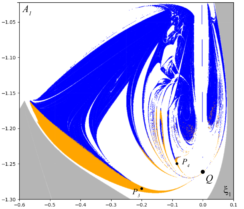
Figure 3: Lyapunov diagram for system (3) in the parameter plane $(\xi_{1},A_{1})$ for $\xi_{2}=1.81,A_{4}=-0.125$. Regions of the existence of pseudohyperbolic attractors (orange) adjoin to the point $Q:(\xi_{1},A_{1})\approx(0,-1.27)$. The region containing the point $P_{3}$ corresponds to an $S$-symmetric pair of $2$-winged Lorenz attractors, see Fig. 4a, and the region containing the point $P_{4}$ corresponds to a $4$-winged attractor, see Fig. 4b.

On the contrary, in the presence of the 4th harmonic, conditions of the theorem are easily satisfied. For instance, for the coupling function $g$ given by formula (2) with $A_{4}=-0.125$, the splay-phase state $O$ has three eigenvalues at $A_{1}=-1$, $\xi_{1}=0$, $\xi_{2}=\arccos\left(-0.25\right)\approx 1.823$, and inequalities (Triple instability and robust chaos.) are fulfilled. Therefore, system (3) has robustly chaotic attractors for $\xi_{2}$ close to $\arccos(-0.25)$ from below.

In Fig. 3, we show the regions of the existence of pseudohyperbolic attractors in the $(\xi_{1},A_{1})$-plane for $\xi_{2}=1.81$, $A_{4}=-0.125$. To plot this diagram, we repeated the same experiment as was done for Fig. 1, but with the initial conditions $(\theta_{1},\theta_{2},\theta_{3})=(1.57,3.14,4.71)$ (near the splay-phase state $O$), and the tolerance bounds equal to $0.001$ for the Lyapunov exponents and $0.03$ for the angle $\alpha$ between the Lyapunov subspaces. The diagram is consistent with that for the theoretical normal form, see Fig. 6 in Ref. [43]. In particular, there are several regions corresponding to the 2-winged and 4-winged pseudohyperbolic attractors, see Fig. 4. In agreement with Theorem 1.3 of Ref. [44], these regions adjoin to the same point $Q:(\xi_{1},A_{1})\approx(0,-1.2625)$.

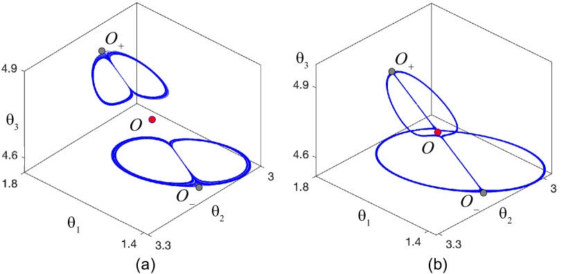
Figure 4: (a) a pair of 2-winged Lorenz attractors at $P_{3}:(\xi_{1},A_{1})=(-0.2,-1.285)$; (b) a 4-winged Lorenz-like attractor at $P_{4}:(\xi_{1},A_{1})=(-0.085,-1.25)$.

Conclusion.

There are two types of chaotic attractors: for pseudohyperbolic attractors every orbit has positive top Lyapunov exponent and this property is robust with respect to small perturbations, and if the pseudohyperbolicity is violated, then only a typical orbit has positive top Lyapunov exponent and small perturbations can destroy chaos and create stable periodic orbits. Numerically, the pseudohyperbolicity (hence – robust chaos) can be reliably verified by augmenting the computation of Lyapunov exponents with the evaluation of angles between Lyapunov subspaces. We gave rigorous analytic conditions for the emergence of pseudohyperbolic attractors in a system of 4 globally coupled identical phase oscillators due to a triple instability bifurcation of the splay-phase synchronization state. The existence, in the space of parameters of the system, of open regions of robustly chaotic behavior was confirmed numerically.

The robustness implies that the found chaotic attractors survive any small changes in the coupling function, as well as the frequency detuning, breaking the symmetry of the coupling, etc. An important general fact is that weakly coupled identical systems with pseudohyperbolic attractors also have pseudohyperbolic attractors. Therefore, our results imply that any network of 4-oscillator systems of the type studied here also has pseudohyperbolic attractors, provided the interaction between the 4-oscillator clusters is weak enough. In this way, one can create large ensembles of weakly-interacting identical oscillators that demonstrate robustly chaotic behavior.

References

- Izhikevich [2007] E. Izhikevich, Dynamical systems in neuroscience (MIT press, 2007).
- Ashwin et al. [2016] P. Ashwin, S. Coombes, and R. Nicks, Mathematical frameworks for oscillatory network dynamics in neuroscience, The Journal of Mathematical Neuroscience 6, 1 (2016).
- Taylor et al. [2022] J. D. Taylor, A. S. Chauhan, J. T. Taylor, A. L. Shilnikov, and A. Nogaret, Noise-activated barrier crossing in multiattractor dissipative neural networks, Physical Review E 105, 064203 (2022).
- Richard et al. [1996] P. Richard, B. M. Bakker, B. Teusink, K. Van Dam, and H. V. Westerhoff, Acetaldehyde mediates the synchronization of sustained glycolytic oscillations in populations of yeast cells, European journal of biochemistry 235, 238 (1996).
- Prindle et al. [2012] A. Prindle, P. Samayoa, I. Razinkov, T. Danino, L. S. Tsimring, and J. Hasty, A sensing array of radically coupled genetic “biopixels”, Nature 481, 39 (2012).
- Peskin [1975] C. S. Peskin, Mathematical aspects of heart physiology, Courant Inst. Math (1975).
- Garashchuk et al. [2020] I. R. Garashchuk, A. O. Kazakov, and D. I. Sinelshchikov, Synchronous oscillations and symmetry breaking in a model of two interacting ultrasound contrast agents, Nonlinear Dynamics 101, 1199 (2020).
- Kuramoto [1984] Y. Kuramoto, Chemical oscillations, waves, and turbulence (Springer Berlin, Heidelberg, 1984).
- Taylor et al. [2009] A. Taylor, M. Tinsley, Z. Huang, and K. Showalter, Dynamical quorum sensing and synchronization in large populations of chemical oscillators, science 323, 614 (2009).
- Toiya et al. [2010] M. Toiya, H. O. González-Ochoa, V. K. Vanag, S. Fraden, and I. R. Epstein, Synchronization of chemical micro-oscillators, The Journal of Physical Chemistry Letters 1, 1241 (2010).
- Yan et al. [2012] J. Yan, M. Bloom, S. C. Bae, E. Luijten, and S. Granick, Linking synchronization to self-assembly using magnetic Janus colloids, Nature 491, 578 (2012).
- Kourtchatov et al. [1995] S. Y. Kourtchatov, V. Likhanskii, A. Napartovich, F. Arecchi, and A. Lapucci, Theory of phase locking of globally coupled laser arrays, Physical Review A 52, 4089 (1995).
- Kozyreff et al. [2000] G. Kozyreff, A. Vladimirov, and P. Mandel, Global coupling with time delay in an array of semiconductor lasers, Physical Review Letters 85, 3809 (2000).
- Takemura et al. [2020] N. Takemura, M. Takiguchi, and M. Notomi, Designs toward synchronization of optical limit cycles with coupled silicon photonic crystal microcavities, Optics Express 28, 27657 (2020).
- Benz and Burroughs [1991] S. P. Benz and C. J. Burroughs, Coherent emission from two-dimensional Josephson junction arrays, Applied physics letters 58, 2162 (1991).
- Wiesenfeld et al. [1998] K. Wiesenfeld, P. Colet, and S. H. Strogatz, Frequency locking in Josephson arrays: Connection with the Kuramoto model, Physical Review E 57, 1563 (1998).
- Mukhopadhyay et al. [2023] S. Mukhopadhyay, J. Senior, J. Saez-Mollejo, D. Puglia, M. Zemlicka, J. M. Fink, and A. P. Higginbotham, Superconductivity from a melted insulator in Josephson junction arrays, Nature Physics 19, 1630 (2023).
- Martens et al. [2013] E. A. Martens, S. Thutupalli, A. Fourriere, and O. Hallatschek, Chimera states in mechanical oscillator networks, Proceedings of the National Academy of Sciences 110, 10563 (2013).
- Belykh et al. [2017] I. Belykh, R. Jeter, and V. Belykh, Foot force models of crowd dynamics on a wobbly bridge, Science advances 3, e1701512 (2017).
- Belykh et al. [2021] I. Belykh, M. Bocian, A. R. Champneys, K. Daley, R. Jeter, J. H. Macdonald, and A. McRobie, Emergence of the London Millennium Bridge instability without synchronisation, Nature communications 12, 7223 (2021).
- Turing [1952] A. M. Turing, The chemical basis of morphogenesis, Bulletin of mathematical biology 52, 153 (1952).
- Smale [1976] S. Smale, A mathematical model of two cells via Turing’s equation, in The Hopf bifurcation and its applications (Springe, 1976) pp. 354–367.
- Drubi et al. [2007] F. Drubi, S. Ibanez, and A. Rodriguez, Coupling leads to chaos, Journal of Differential Equations 239, 371 (2007).
- Nijholt et al. [2023] E. Nijholt, T. Pereira, F. Queiroz, and D. Turaev, Chaotic behavior in diffusively coupled systems, Communications in Mathematical Physics 401, 2715 (2023).
- Ashwin and Swift [1992] P. Ashwin and J. W. Swift, The dynamics of weakly coupled identical oscillators, Journal of Nonlinear Science 2, 69 (1992).
- Swift et al. [1992] J. W. Swift, S. H. Strogatz, and K. Wiesenfeld, Averaging of globally coupled oscillators, Physica D: Nonlinear Phenomena 55, 239 (1992).
- Winfree [1967] A. T. Winfree, Biological rhythms and the behavior of populations of coupled oscillators, Journal of theoretical biology 16, 15 (1967).
- Kuramoto [1975] Y. Kuramoto, Self-entrainment of a population of coupled non-linear oscillators, in International Symposium on Mathematical Problems in Theoretical Physics (Springer, 1975) pp. 420–422.
- Afraimovich et al. [1986] V. Afraimovich, N. Verichev, and M. I. Rabinovich, Stochastic synchronization of oscillation in dissipative systems, Radiophysics and Quantum Electronics 29, 795 (1986).
- Berner et al. [2023] R. Berner, A. Lu, and I. M. Sokolov, Synchronization transitions in kuramoto networks with higher-mode interaction, Chaos: An Interdisciplinary Journal of Nonlinear Science 33 (2023).
- Sakaguchi and Kuramoto [1986] H. Sakaguchi and Y. Kuramoto, A soluble active rotater model showing phase transitions via mutual entertainment, Progress of Theoretical Physics 76, 576 (1986).
- Ashwin and Rodrigues [2016] P. Ashwin and A. Rodrigues, Hopf normal form with symmetry and reduction to systems of nonlinearly coupled phase oscillators, Physica D: Nonlinear Phenomena 325, 14 (2016).
- Watanabe and Strogatz [1993] S. Watanabe and S. H. Strogatz, Integrability of a globally coupled oscillator array, Physical Review Letters 70, 2391 (1993).
- Strogatz [2000] S. H. Strogatz, From Kuramoto to Crawford: exploring the onset of synchronization in populations of coupled oscillators, Physica D 143, 1 (2000).
- Watanabe and Strogatz [1994] S. Watanabe and S. H. Strogatz, Constants of motion for superconducting Josephson arrays, Physica D: Nonlinear Phenomena 74, 197 (1994).
- Ashwin et al. [2007] P. Ashwin, G. Orosz, J. Wordsworth, and S. Townley, Dynamics on networks of cluster states for globally coupled phase oscillators, SIAM Journal on Applied Dynamical Systems 6, 728 (2007).
- Bick et al. [2011] C. Bick, M. Timme, D. Paulikat, D. Rathlev, and P. Ashwin, Chaos in symmetric phase oscillator networks, Physical Review Letters 107, 244101 (2011).
- Bick et al. [2016] C. Bick, P. Ashwin, and A. Rodrigues, Chaos in generically coupled phase oscillator networks with nonpairwise interactions, Chaos: An Interdisciplinary Journal of Nonlinear Science 26 (2016).
- Arefev et al. [2023] A. Arefev, E. Grines, and G. Osipov, Heteroclinic cycles and chaos in a system of four identical phase oscillators with global biharmonic coupling, Chaos: An Interdisciplinary Journal of Nonlinear Science 33 (2023).
- Grines et al. [2022] E. A. Grines, A. Kazakov, and I. R. Sataev, On the origin of chaotic attractors with two zero Lyapunov exponents in a system of five biharmonically coupled phase oscillators, Chaos: An Interdisciplinary Journal of Nonlinear Science 32 (2022).
- Afraimovich and Shilnikov [1983] V. S. Afraimovich and L. P. Shilnikov, Strange attractors and quasiattractors, in Nonlinear Dynamics and Turbulence, edited by G. I. Barenblatt, G. Iooss, and D. D. Joseph , 1 (1983).
- Gonchenko et al. [2021a] S. Gonchenko, A. Kazakov, and D. Turaev, Wild pseudohyperbolic attractor in a four-dimensional Lorenz system, Nonlinearity 34, 2018 (2021a).
- Karatetskaia et al. [2025a] E. Karatetskaia, A. Kazakov, K. Safonov, and D. Turaev, Multi-winged Lorenz attractors due to bifurcations of a periodic orbit with multipliers , Nonlinearity (2025a).
- Karatetskaia et al. [2025b] E. Karatetskaia, A. Kazakov, K. Safonov, and D. Turaev, Analytic proof of the emergence of new type of Lorenz-like attractors from the triple instability in systems with -symmetry, Journal of Differential Equations (2025b).
- Turaev and Shilnikov [1998] D. V. Turaev and L. P. Shilnikov, An example of a wild strange attractor, Sbornik: Mathematics 189, 291 (1998).
- Kuptsov and Parlitz [2012] P. V. Kuptsov and U. Parlitz, Theory and computation of covariant Lyapunov vectors, Journal of nonlinear science 22, 727 (2012).
- Ginelli et al. [2013] F. Ginelli, H. Chaté, R. Livi, and A. Politi, Covariant Lyapunov vectors, Journal of Physics A: Mathematical and Theoretical 46, 254005 (2013).
- Pikovsky and Politi [2016] A. Pikovsky and A. Politi, Lyapunov exponents: a tool to explore complex dynamics (Cambridge University Press, 2016).
- Oseledets [1968] V. Oseledets, A multiplicative ergodic theorem. Characteisitic Lyapunov, exponents of dynamical systems, Tr. Mosk. Mat. Obs 19, 179 (1968).
- Bonatti et al. [2004] C. Bonatti, L. J. Díaz, and M. Viana, Dynamics beyond uniform hyperbolicity: A global geometric and probabilistic perspective, Vol. 3 (Springer Science & Business Media, 2004).
- Turaev and Shilnikov [2008] D. Turaev and L. Shilnikov, Pseudohyperbolicity and the problem on periodic perturbations of Lorenz-type attractors, Doklady Mathematics 77, 17 (2008).
- Anosov et al. [1995] D. Anosov, G. Gould, S. Aranson, V. Grines, R. Plykin, A. Safonov, E. Sataev, S. Shlyachkov, V. Solodov, A. Starkov, et al., Dynamical systems IX: dynamical systems with hyperbolic behaviour, Vol. 66 (Springer, 1995).
- Pesin and Sinai [1982] Y. B. Pesin and Y. G. Sinai, Gibbs measures for partially hyperbolic attractors, Ergodic Theory and Dynamical Systems 2, 417 (1982).
- Kuznetsov [2005] S. P. Kuznetsov, Example of a physical system with a hyperbolic attractor of the Smale-Williams type, Physical review letters 95, 144101 (2005).
- Lorenz [1963] E. N. Lorenz, Deterministic nonperiodic flow, Journal of atmospheric sciences 20, 130 (1963).
- Guckenheimer and Williams [1979] J. Guckenheimer and R. F. Williams, Structural stability of Lorenz attractors, Publications Mathématiques de l’IHÉS 50, 59 (1979).
- Afraimovich et al. [1977] V. S. Afraimovich, V. Bykov, and L. P. Shilnikov, On the origin and structure of the Lorenz attractor, Akademiia Nauk SSSR Doklady 234, 336 (1977).
- Afraimovich et al. [1982] V. S. Afraimovich, V. Bykov, and L. P. Shilnikov, Attractive nonrough limit sets of Lorenz-attractor type, Trudy Moskovskoe Matematicheskoe Obshchestvo 44, 150 (1982).
- Tucker [1999] W. Tucker, The Lorenz attractor exists, Comptes Rendus de l’Académie des Sciences-Series I-Mathematics 328, 1197 (1999).
- Gonchenko et al. [2021b] S. Gonchenko, A. Gonchenko, A. Kazakov, and E. Samylina, On discrete Lorenz-like attractors, Chaos: An Interdisciplinary Journal of Nonlinear Science 31 (2021b).
- Gonchenko et al. [2022] S. Gonchenko, E. Karatetskaia, A. Kazakov, and V. Kruglov, Conjoined Lorenz twins – a new pseudohyperbolic attractor in three-dimensional maps and flows, Chaos: An Interdisciplinary Journal of Nonlinear Science 32 (2022).
- Barros et al. [2024] D. Barros, C. Bonatti, and M. J. Pacifico, Upper, down, two-sided Lorenz attractor, collisions, merging, and switching, Ergodic Theory and Dynamical Systems , 1 (2024).
- Kazakov et al. [2024] A. Kazakov, A. Murillo, A. Vieiro, and K. Zaichikov, Numerical study of discrete Lorenz-like attractors, Regular and Chaotic Dynamics 29, 78 (2024).
- Gonchenko et al. [2005] S. V. Gonchenko, I. Ovsyannikov, C. Simó, and D. Turaev, Three-dimensional Hénon-like maps and wild Lorenz-like attractors, International Journal of Bifurcation and Chaos 15, 3493 (2005).
- Newhouse [1974] S. E. Newhouse, Diffeomorphisms with infinitely many sinks, Topology 13, 9 (1974).
- Gonchenko et al. [2008] S. V. Gonchenko, L. P. Shilnikov, and D. V. Turaev, On dynamical properties of multidimensional diffeomorphisms from Newhouse regions: I, Nonlinearity 21, 923 (2008).
- Kuptsov [2012] P. V. Kuptsov, Fast numerical test of hyperbolic chaos, Physical Review E – Statistical, Nonlinear, and Soft Matter Physics 85, 015203 (2012).
- Kuptsov and Kuznetsov [2018] P. V. Kuptsov and S. P. Kuznetsov, Lyapunov analysis of strange pseudohyperbolic attractors: angles between tangent subspaces, local volume expansion and contraction, Regular and Chaotic Dynamics 23, 908 (2018).
- Gonchenko et al. [2021c] S. V. Gonchenko, M. Kaynov, A. O. Kazakov, and D. V. Turaev, On methods for verification of the pseudohyperbolicity of strange attractors, Izvestiya VUZ. Applied Nonlinear Dynamics 29, 160 (2021c).
- Ruelle [1981] D. Ruelle, Small random perturbations of dynamical systems and the definition of attractors, Communications in Mathematical Physics 82, 137 (1981).
- Gonchenko and Turaev [2017] S. V. Gonchenko and D. V. Turaev, On three types of dynamics and the notion of attractor, Proceedings of the Steklov Institute of Mathematics 297, 116 (2017).