Heat as a witness of quantum properties
Abstract
We present a new approach for witnessing quantum resources, including entanglement and coherence, based on heat generation. Inspired by the concept of Maxwell’s demon, we analyze the heat exchange between a quantum system and a thermal environment assisted by a quantum memory. By exploring the fundamental limitations of heat transfer in this scenario, we find that quantum states can reveal their non-classical signatures via energy exchange with a thermal environment. This approach offers a promising alternative to complex, system-specific measurements, as it relies solely on fixed energy measurements. To demonstrate the effectiveness of our method, we apply it to the detection of entanglement in isotropic states and coherence in a two-spin system interacting with a single-mode electromagnetic field.
I Introduction
Thermodynamics and information theory are fundamentally intertwined. A notable example highlighting this connection is the concept of Maxwell’s demon [1]. This thought experiment introduces an imaginary agent capable of sorting gas molecules by their velocities. By creating a temperature difference, the demon apparently defies the second law of thermodynamics, decreasing the system’s entropy without expending energy. The paradox is resolved by considering the demon’s memory: erasing the stored information, which is necessary to complete a thermodynamically cyclic process, inevitably generates heat and increases entropy, in accordance with Landauer’s principle [2, 3, 4].
In modern stochastic thermodynamics, Maxwell’s demon is regarded as a thermodynamic protocol incorporating measurement and feedback control [5, 6, 7]. The demon is an agent with the capacity to measure a thermodynamic system, store its measurement outcomes in a memory, and then use them to implement a feedback process. Importantly, the demon’s memory is typically seen as a classical system, one whose state can be fully described using orthogonal quantum states.
Recent progress both in theory [8] and technology [9, 10, 11] for storing quantum information naturally leads to the question of whether the quantum nature of the memory system can be harnessed in the operation of Maxwell’s demon. Such a generalization opens up possibilities for using the memory in new and interesting ways. Beyond storing classical information, ancillary quantum systems have the potential to store “unspeakable” information that cannot be transmitted through classical communication channels [12]. These ancillary systems act as reference frames [13, 14, 15], such as phase references [16]. Furthermore, quantum memories can become entangled with the system, leading to dynamics that cannot be explained solely by classical memory systems [17].
In this work we consider a quantum version of the Maxwell’s demon [18, 19, 20], namely a demon with a quantum memory that can be initialized in any quantum state. We show that such demons can surprisingly generate heat flows that exceed the limits of classical heat exchange. Within this broader scenario, we derive fundamental constraints on heat exchange in thermodynamic processes such as cooling and heating.
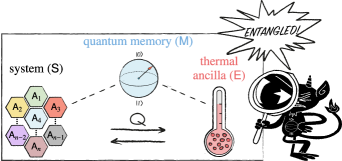
Our results reveal a fundamental correspondence between thermodynamic quantities and quantum features. More precisely, we demonstrate that the quantum nature of the system manifests in its heat exchange with the surrounding thermal environment. We identify distinct thermal signatures associated with quantum properties, including entanglement and coherence. This presents a novel approach for detecting quantum features via heat exchange during a thermodynamic process (see Fig. 1 for a schematic representation). This method replaces system-specific measurements with a simpler energy measurement on a thermal ancilla. To illustrate the effectiveness of this technique, we provide two examples: First, we show entanglement detection for two-qubit Werner states; Second, we propose an experimentally feasible protocol for certifying the coherence of spins interacting with a single-mode electromagnetic field.
II Preliminaries
We consider a setup comprising three parts: a main system S, a memory system M and an environment E (see Fig. 1). Each subsystem is described by its local Hamiltonian of dimension , where indicates the -th energy eigenvalue and the corresponding eigenstate of subsystem . Without loss of generality, we assume that the energies are sorted in increasing order, i.e., for all . The main system and memory starts in arbitrary states and , while the enviroment is initially in a thermal (Gibbs) state at inverse temperature , with denoting the Boltzmann constant. We use natural units where
We aim to characterize the maximum and minimum amount of heat that the system can exchange with the environment E at a given temperature when using M as a (quantum) memory system. To ensure that heat is delivered exclusively due to the system S, we need to make two additional assumptions. First, the joint system SRE is assumed to be closed and evolves via an energy-preserving unitary process as [21]
| (1) |
where satisfies . Since there are no extra sources of energy, the energy exchange between the system SR and the environment E can be considered as heat , where . Second, we demand that the memory M does not transfer energy to the system SE. This is achieved by imposing that M does not change under the dynamics, i.e.,
| (2) |
In other words, system M acts as a (quantum) memory, i.e., affects the dynamics of the system but not its energetics. This setting includes the scenario of Maxwell’s daemon with feedbacks [22, 23, 24], with the important distinction that here the control system is genuinely quantum. Note that, due to the Naimark’s theorem [25], any measurement and feedback protocol that restores the memory to its original state without requiring work can be implemented by an appropriate choice of and . Consequently, our framework encompasses, but is not restricted to, the standard Maxwell’s demon scenario. Finally, Eq. (2) indicates that the memory undegoes a cyclic evolution. While this process can be equivalently viewed as a catalytic evolution [26, 27], we emphasize that the memory is not reused in the process. For this reason, we refer to it as the “memory” throughout this paper.
The above assumptions allow us to define the maximal and minimal amounts of heat that can be transferred to any environment under any energy-preserving interaction, namely
| (3) | ||||
The index denotes the minimal and maximal heat for cooling and heating the environment, respectively.
We emphasize that our motivation is to quantify heat without making additional assumptions about the underlying model or its dynamical complexity. Therefore, we make no additional assumptions about the interaction’s strength (whether it is weak or strong), its complexity (local or collective), or its duration (short or long) relative to the natural time scales. Similarily, we make no assumptions about the thermal environment.
III Optimal heat transfer with quantum memory
To facilitate analysis we recast the optimisation problem from Eq. (3) into a simpler form. Let us denote the quantum free energy by , where and is the von-Neumann entropy. Using techniques from the resource theory of quantum thermodynamics [21, 28], we demonstrate in Appendix A that Eq. (3) can be reformulated as a convex optimisation problem over density operators, namely
| (4) | ||||
where . Note that the system can provide at most energy to the environment, hence . This happens when or .
The problem from Eq. (4) can be solved directly using Jaynes’s principle [29]. Specifically, consider the function
| (5) |
where and . In Appendix A-3, we show that the solution of the problem from Eq. (4) can be expressed as
| (6) | ||||
| (7) |
where the inverse temperatures are given by the zeros of the function chosen such that . These quantities specify the minimal and maximal amount of heat that a system can transfer to a thermal environment with the help of a quantum memory.
IV Certifying properties of quantum states via heat transfer
The heat flow between the system S and the environment E, mediated by the memory M, can reveal interesting properties of the quantum state of the system. To see this, let denote a fixed set of quantum states and consider
| (8) |
Any quantum state satisfies . This observation can be used to construct a witness for the set . Specifically, if we observe a state that releases or accepts heat with a magnitude greater than , we can be certain that the state did not belong to in the first place.
While directly computing the actual values can be difficult, often we can obtain useful bounds by exploiting specific properties of the set . For that, suppose we find a bound on the maximal free energy of states inside the set , namely . Then using Eq. (6), we find
| (9) |
The inverse temperature is given by the (largest) zero of the function . Similarly, is defined using the smallest zero of . In the following sections, this technique will be used to certify entanglement and coherence in quantum systems. We highlight that the presented method is rather general and can be used to certify also other properties of quantum states.
V Example 1: Entanglement witnessing
As a first example, we show that entanglement of a bipartite system can be witnessed by measuring the heat it transfers to the environment.
Let be a bipartite quantum system and be the set of separable bipartite states, i.e., the convex hull of product states between A and B [30]. To construct a witness for the set (entanglement witness), we first need to establish a bound on that is valid for all separable states. Observe that , where is the quantum mutual information and is the quantum conditional entropy [31, 32, 33]. Interestingly, the quantum conditional entropy is positive for all separable states [31, 34]. This allows us to establish the following (tight) bound:
| (10) |
Using this, we can construct a heat-based entanglement witness, namely , where
| (11) |
with as the inverse temperatures that correspond to the zeros of the function . Observe that the entanglement witness defined in Eq. (11) can detect any bipartite pure entangled state of arbitrary dimension. This is because the quantum conditional entropy of such states is always negative [35].
One can also use Eq. (11) to certify entanglement of general bipartite states. To demonstrate this we discuss an example involving two-qudit isotropic states with [36]:
| (12) |
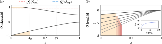
where , and is the identity operator on AB. It is known that isotropic states are entangled for [37]. We begin by analysing heat flow in the particular case of , where Eq. (12) reduces to the well-known family of Werner states. In Figure 2a, we plot as a function of and compare it with . It can be observed that both and detect entanglement up to a critical value which is precisely when the conditional entropy becomes positive.
The critical value specifies the range of isotropic states that can be witnessed using our techniques. In Appendix B, we show that is specified by a transcendental equation that relates it to the local dimension . The interplay between the heat exchange, local dimension, and is depicted in Fig. 2b. More precisely, we plot the heat exchange for different values of alongside the respective bounds (depicted by the colored region). We observe that as the local dimension increases, the detection improves, which depends on . To gain insight into the dependence of as a function of the local dimension, we show its behavior in the inset of Fig. 2b. As noted, for larger , approaches an asymptotic value .
We point out that when constructing our entanglement witness, we assumed that the local entropies and (average) energies are known. The construction can be easily generalized to the case when local entropies and energies are known only to a fixed precision. Furthermore, more general bounds that do not rely on this information can also be derived. Specifically, by using in Eq. (V), we can obtain more general (but typically looser) bounds on . Moreover, our analysis can be extended to witnessing multipartite entangled states, as shown in Appendix C. Finally, the techniques presented here also allow witnessesing classical correlations. In this case one would simply use a different bound in Eq. (V), e.g. using the fact that for uncorrelated states.
VI Example 2: Certification of Quantum Coherence
Our second example illustrate how to construct a heat-based witness for certifying the presence of quantum coherence.
Let be the set of states incoherent (i.e. diagonal) in the energy eigenbasis with a fixed average energy . Furthermore, define to be the state of S dephased in its energy basis. Our goal is to find an appropriate bound and then use it to construct witnesses for quantum coherence.
We start by observing that , where is the relative entropy of coherence [38, 15, 39]. Crucially, for all incoherent states and positive only for coherent ones. In order to find , we observe that the maximum is achieved by an incoherent state that minimises entropy under fixed average energy . Such a state is simply given by with . This allows us to find the following (tight) bound
| (13) |
where is the binary entropy. Using Eq. (13) we can construct a heat-based coherence witness, namely , where
| (14) |
where are specified by the zeros of .
We now illustrate how our witness performs in a realistic scenario. Consider two spins (two-level systems) S and E with the same energy gap and energy levels for , coupled to a single mode electromagnetic field M with frequency . Furthermore, let denote the bosonic annihilation operator of the field and be the lowering operator of spin X. The two spins S and E should be understood, respectively, as the main system and environment, while the field M plays the role of the memory system. The joint system then evolves via the Tavis-Cummings Hamiltonian [40], which in the rotating wave approximation reads
| (15) |
where and specifies the coupling strength. Notice further that and, moreover, the system S cannot directly transfer energy to the thermal environment E but only through the memory M.
The system is prepared in a state with coherence , where , while the environment starts in a Gibbs state . Finally, the field is prepared in a state which will be determined as follows. At time the interaction is turned on and the spins interact with the field for a fixed time . This evolution is described by a unitary and leads to
| (16) |
Since we want the field to act only as a control system, it must satisfy . This is a well-defined operator equation that can be solved numerically using various techniques, e.g. semi-definite programming [41]. The state of the field is then chosen to be the solution of this equation, meaning that the field returns to its initial state at time . This reasoning is valid for any .
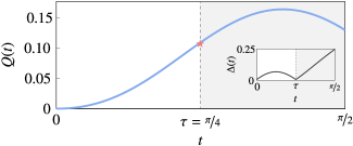
The heat exchanged in the process as a function of time is shown in Fig. 3. It can be easily verified that in our example the bounds on heat are zero, , since the dephased state is a Gibbs state. Consequently, the presence of coherence can be inferred by monitoring . It is worth noting that this behavior would be impossible if the control system were classical and lacked energy coherences. Remarkably, the quantum nature of the memory system provides a way to access the correlations “locked” in the non-degenerate energy subspaces theareby boosting the energy flow between the subsystems [42, 43].
VII Discussion and Outlook
In this work we have established a fundamental link between thermodynamics and quantum features. We demonstrated that quantum properties can be detected by monitoring the heat exchange in a quantum process. Our approach is inspired by the Maxwell’s demon thought experiment, where the classical memory is replaced by a quantum one.
To illustrate our results, we considered two case studies: entanglement detection in bipartite systems and coherence certification in a three-level system. Importantly, our methods are not limited to these examples and can be used more broadly, i.e., to certify other properties of quantum states.
Our results could be potentially implemented in state-of-the-art experimental setups, such as those utilizing nuclear magnetic resonance techniques [44, 45] or ion trap technology [46, 47]. Beyond proof-of-principle experiments, it would be interesting to investigate whether the techniques presented here offer practical advantages for entanglement or coherence certification. Specifically in the entanglement case, it would be interesting to to quantify the sample complexity of this entanglement witnessing procedure, comparing it with existing state-of-the-art techniques in the field.
Finally, we highlight that the concepts discussed here can be framed as a catalytic transformation [26, 27], with the quantum memory being the catalyst. Therefore, our findings demonstrate a concrete application for the concept of quantum catalysis. This contrasts with the typical abstract treatment of catalysts within the resource-theoretic framework [48].
Acknowledgements.
AOJ and JBB acknowledges financial support from the Danish National Research Foundation grant bigQ (DNRF 142) and VILLUM FONDEN through a research grant (40864). P.L.-B. acknowledges the Swiss National Science Foundation for financial support through the NCCR SwissMAP.References
- Maxwell [1984] J. C. Maxwell, Theory of heat (Longmans, Green, and Co., 1984).
- Landauer [1961] R. Landauer, Irreversibility and heat generation in the computing process, IBM J. Res. Dev. 5, 183 (1961).
- Reeb and Wolf [2014] D. Reeb and M. M. Wolf, An improved landauer principle with finite-size corrections, New J. Phys. 16, 103011 (2014).
- Plenio and Vitelli [2001] M. B. Plenio and V. Vitelli, The physics of forgetting: Landauer’s erasure principle and information theory, Contemp. Phys 42, 25 (2001).
- Parrondo et al. [2015] J. M. Parrondo, J. M. Horowitz, and T. Sagawa, Thermodynamics of information, Nat. Phys 11, 131 (2015).
- Esposito and Schaller [2012] M. Esposito and G. Schaller, Stochastic thermodynamics for “maxwell demon” feedbacks, EPL 99, 30003 (2012).
- Sagawa and Ueda [2008] T. Sagawa and M. Ueda, Second law of thermodynamics with discrete quantum feedback control, Phys. Rev. Lett. 100, 080403 (2008).
- Rosset et al. [2018] D. Rosset, F. Buscemi, and Y.-C. Liang, Resource theory of quantum memories and their faithful verification with minimal assumptions, Phys. Rev. X 8, 021033 (2018).
- Simon et al. [2010] C. Simon, M. Afzelius, J. Appel, A. Boyer de la Giroday, S. J. Dewhurst, N. Gisin, C. Y. Hu, F. Jelezko, S. Kröll, J. H. Müller, J. Nunn, E. S. Polzik, J. G. Rarity, H. De Riedmatten, W. Rosenfeld, A. J. Shields, N. Sköld, R. M. Stevenson, R. Thew, I. A. Walmsley, M. C. Weber, H. Weinfurter, J. Wrachtrup, and R. J. Young, Quantum memories: A review based on the european integrated project “qubit applications (qap)”, Eur. Phys. J. D 58, 1–22 (2010).
- Lvovsky et al. [2009] A. I. Lvovsky, B. C. Sanders, and W. Tittel, Optical quantum memory, Nat. Photonics 3, 706 (2009).
- Heshami et al. [2016] K. Heshami, D. G. England, P. C. Humphreys, P. J. Bustard, V. M. Acosta, J. Nunn, and B. J. Sussman, Quantum memories: emerging applications and recent advances, J. Mod. Opt 63, 2005–2028 (2016).
- Marvian and Spekkens [2016] I. Marvian and R. W. Spekkens, How to quantify coherence: Distinguishing speakable and unspeakable notions, Phys. Rev. A 94, 052324 (2016).
- Bartlett et al. [2007] S. D. Bartlett, T. Rudolph, and R. W. Spekkens, Reference frames, superselection rules, and quantum information, Rev. Mod. Phys. 79, 555 (2007).
- Giacomini et al. [2019] F. Giacomini, E. Castro-Ruiz, and C. Brukner, Quantum mechanics and the covariance of physical laws in quantum reference frames, Nat. Commun 10, 494 (2019).
- Lostaglio et al. [2015] M. Lostaglio, D. Jennings, and T. Rudolph, Description of quantum coherence in thermodynamic processes requires constraints beyond free energy, Nat. Commun 6, 6383 (2015).
- Streltsov et al. [2017] A. Streltsov, G. Adesso, and M. B. Plenio, Colloquium: Quantum coherence as a resource, Rev. Mod. Phys. 89, 041003 (2017).
- Rio et al. [2011] L. d. Rio, J. Åberg, R. Renner, O. Dahlsten, and V. Vedral, The thermodynamic meaning of negative entropy, Nature 474, 61–63 (2011).
- Cottet et al. [2017] N. Cottet, S. Jezouin, L. Bretheau, P. Campagne-Ibarcq, Q. Ficheux, J. Anders, A. Auffèves, R. Azouit, P. Rouchon, and B. Huard, Observing a quantum maxwell demon at work, PNAS 114, 7561 (2017).
- Naghiloo et al. [2018] M. Naghiloo, J. J. Alonso, A. Romito, E. Lutz, and K. W. Murch, Information gain and loss for a quantum maxwell’s demon, Phys. Rev. Lett. 121, 030604 (2018).
- Masuyama et al. [2018] Y. Masuyama, K. Funo, Y. Murashita, A. Noguchi, S. Kono, Y. Tabuchi, R. Yamazaki, M. Ueda, and Y. Nakamura, Information-to-work conversion by maxwell’s demon in a superconducting circuit quantum electrodynamical system, Nat. Commun. 9, 1291 (2018).
- Janzing et al. [2000] D. Janzing, P. Wocjan, R. Zeier, R. Geiss, and T. Beth, Thermodynamic cost of reliability and low temperatures: Tightening landauer’s principle and the second law, Int. J. Theor. Phys. 39, 2717 (2000).
- Sagawa and Ueda [2012] T. Sagawa and M. Ueda, Fluctuation theorem with information exchange: Role of correlations in stochastic thermodynamics, Phys. Rev. Lett. 109, 180602 (2012).
- Ito and Sagawa [2015] S. Ito and T. Sagawa, Maxwell’s demon in biochemical signal transduction with feedback loop, Nat. Commun 6, 1 (2015).
- Seifert [2012] U. Seifert, Stochastic thermodynamics, fluctuation theorems and molecular machines, Rep. Prog. Phys 75, 126001 (2012).
- Nielsen and Chuang [2001] M. A. Nielsen and I. L. Chuang, Quantum computation and quantum information, Vol. 2 (Cambridge university press Cambridge, 2001).
- Datta et al. [2023] C. Datta, T. V. Kondra, M. Miller, and A. Streltsov, Catalysis of entanglement and other quantum resources, Rep. Prog. Phys. 86, 116002 (2023).
- Lipka-Bartosik et al. [2024a] P. Lipka-Bartosik, H. Wilming, and N. H. Y. Ng, Catalysis in quantum information theory, Rev. Mod. Phys. 96, 025005 (2024a).
- Horodecki and Oppenheim [2013] M. Horodecki and J. Oppenheim, Fundamental limitations for quantum and nanoscale thermodynamics, Nat. Commun. 4, 2059 (2013).
- Jaynes [1957] E. T. Jaynes, Information theory and statistical mechanics, Phys. Rev 106, 620 (1957).
- Watrous [2018] J. Watrous, The theory of quantum information (Cambridge university press, 2018).
- Cerf and Adami [1997] N. J. Cerf and C. Adami, Negative entropy in quantum information theory (Springer, 1997).
- Cerf and Adami [1998] N. J. Cerf and C. Adami, Information theory of quantum entanglement and measurement, Physica D: Nonlinear Phenomena 120, 62–81 (1998).
- Cerf and Adami [1999] N. J. Cerf and C. Adami, Quantum extension of conditional probability, Phys. Rev. A 60, 893 (1999).
- Vollbrecht and Wolf [2002] K. G. H. Vollbrecht and M. M. Wolf, Conditional entropies and their relation to entanglement criteria, J. Math. Phys. 43, 4299–4306 (2002).
- Friis et al. [2017] N. Friis, S. Bulusu, and R. A. Bertlmann, Geometry of two-qubit states with negative conditional entropy, J. Phys. A: Math. Theor. 50, 125301 (2017).
- Horodecki and Horodecki [1999a] M. Horodecki and P. Horodecki, Reduction criterion of separability and limits for a class of distillation protocols, Phys. Rev. A 59, 4206 (1999a).
- Horodecki and Horodecki [1999b] M. Horodecki and P. Horodecki, Reduction criterion of separability and limits for a class of distillation protocols, Phys. Rev. A 59, 4206 (1999b).
- Janzing [2006] D. Janzing, Quantum thermodynamics with missing reference frames: Decompositions of free energy into non-increasing components, J. Stat. Phys. 125, 761 (2006).
- Winter and Yang [2016] A. Winter and D. Yang, Operational resource theory of coherence, Phys. Rev. Lett. 116, 120404 (2016).
- Tavis and Cummings [1968] M. Tavis and F. W. Cummings, Exact solution for an -molecule—radiation-field hamiltonian, Phys. Rev. 170, 379 (1968).
- Boyd and Vandenberghe [2004] S. Boyd and L. Vandenberghe, Convex Optimization (Cambridge University Press, New York, NY, USA, 2004).
- Lipka-Bartosik et al. [2023] P. Lipka-Bartosik, M. Perarnau-Llobet, and N. Brunner, Operational definition of the temperature of a quantum state, Phys. Rev. Lett. 130, 040401 (2023).
- Lipka-Bartosik et al. [2024b] P. Lipka-Bartosik, G. F. Diotallevi, and P. Bakhshinezhad, Fundamental limits on anomalous energy flows in correlated quantum systems, Phys. Rev. Lett. 132, 140402 (2024b).
- Micadei et al. [2019] K. Micadei, J. P. S. Peterson, A. M. Souza, R. S. Sarthour, I. S. Oliveira, G. T. Landi, T. B. Batalhão, R. M. Serra, and E. Lutz, Reversing the direction of heat flow using quantum correlations, Nat. Commun 10, 10.1038/s41467-019-10333-7 (2019).
- Vandersypen and Chuang [2005] L. M. K. Vandersypen and I. L. Chuang, Nmr techniques for quantum control and computation, Rev. Mod. Phys. 76, 1037 (2005).
- Goold et al. [2014] J. Goold, U. Poschinger, and K. Modi, Measuring the heat exchange of a quantum process, Phys. Rev. E 90, 10.1103/physreve.90.020101 (2014).
- Leibfried et al. [2003] D. Leibfried, R. Blatt, C. Monroe, and D. Wineland, Quantum dynamics of single trapped ions, Rev. Mod. Phys. 75, 281 (2003).
- Chitambar and Gour [2019] E. Chitambar and G. Gour, Quantum resource theories, Rev. Mod. Phys. 91, 025001 (2019).
- Brandão et al. [2015] F. G. S. L. Brandão, M. Horodecki, N. H. Y. Ng, J. Oppenheim, and S. Wehner, The second laws of quantum thermodynamics, Proc. Natl. Acad. Sci. U.S.A. 112, 3275 (2015).
- Lostaglio [2019] M. Lostaglio, An introductory review of the resource theory approach to thermodynamics, Rep. Prog. Phys. 82, 114001 (2019).
- Duan et al. [2005] R. Duan, Y. Feng, X. Li, and M. Ying, Trade-off between multiple-copy transformation and entanglement catalysis, Phys. Rev. A 71, 062306 (2005).
- Feng et al. [2006] Y. Feng, R. Duan, and M. Ying, Relation between catalyst-assisted transformation and multiple-copy transformation for bipartite pure states, Phys. Rev. A 74, 042312 (2006).
Appendix A Optimal heat exchange
We present here the solution to the optimal heat exchange as discussed in Sec. III. This begins by demonstrating that the optimisation problem posed by Eq. (3) can be translated into an equivalent, yet simpler, optimisation problem. We then propose an ansatz for the latter and demonstrate that the optimal heat exchange is given by Eqs. (6) and (7). The focus then shifts to identifying the output thermal state after the process. We show how this equivalent optimisation problem can be reformulated as a problem of determining the solution to an implicit equation. For clarity, the proof is structured into three distinct steps outlined below.
Step 1: Equivalence between optimisation problems
We now present a general proof valid for an -partite system, prepared in a state , where , and described by a Hamiltonian . The optimal amount of heat by which the environment can be either cooled down or warmed up is defined by the following optimisation problem:
| (17) | ||||
General picture illustrating the equivalence
Since solving Eq. (17) is highly non-trivial, we now recast it into a tractable problem. To do so, let us recall some important points. First, due to the catalytic constraint [Eq. (2)], heat is only exchanged between the main system S and the environment E. Second, when S is warmed up, then E is cooled down, and vice versa. Consequently, the minimum heat transferred from the system to the environment corresponds to the maximum heat received by the environment. Third, one can interpret such a process through the perspective of a state transformation undergone by the system , subject to energy conservation and the catalytic constraint. Putting all the pieces together, we can conclude that this is a well-studied class of quantum channels known as thermal operations [49, 28, 50]. In other words, this problem can be framed as a catalytic (coherent) thermal operation that maps to , where , with decaying exponentially with the size of the catalyst. Therefore, one can formulate an equivalent optimisation problem, namely
| (18) | ||||
where is the nonequilibrium free energy with being the relative entropy and is the partition function.
Formal proof
We start by proving that the constraints in Eq. (17) imply . This can be seen by using the unitary invariance property of the von Neumann entropy [3]
| (19) |
where and . Recollecting the terms implies that , which holds true for any choice of operators , and . Next, we assume that and prove that for sufficiently large catalysts, there always exist a choice of operators and that achieves the optimum
We begin by considering the Duan state [51, 52]:
| (20) |
where we denote and . Futhermore, we define where represents the partial trace over the first particles, and is an arbitrary -partite density matrix which will be specified shortly. The unitary is chosen to be
| (21) |
where is a set of unitaries chosen such that for and , which will be further specified. The unitary is a cyclic permutation in the sense that:
| (22) |
with . Up to this point, we still need to specify , and . Note that leads to the global state with of the form
| (23) |
Observe that is energy-preserving as long as is energy preserving on its support. To complete the achievibility proof, we employ the following Lemma:
Lemma 1 (Brandao et. al. [49]).
Let be an arbitrary density matrix and be an arbitrary block-diagonal density matrix. Then, for any , there exists an , a system E, with a Hamiltonian and a state , along with a unitary satisfying and implementing a quantum channel such that
| (24) |
if and only if . Moreover, can be taken to be for some .
From the above result, we know that for any there is a sufficiently large , a system E with Hamiltonian and state , and an energy-preserving unitary acting on the subspace such that
| (25) |
As indicated by the notation, we choose the unitary from Eq. (25) to be the unitary used in the catalytic protocol and the subsystem E to be the environment system whose existance is assured by Lemma 1. This assures that is energy-conserving and that the catalytic constraint is safisfied. Finally, the density matrix is chosen to be
| (26) |
As a result, we arrive at
| (27) |
A straightforward calculation further shows that
| (28) |
i.e. the catalytic constraint is satisfied and the protocol generates arbitrarily small correlations between the catalyst M and system S. Moreover, denoting with the partial trace over systems , we can verify that reads
| (29) |
By construction is close to , with being any state satisfying . Futhermore, Eq. (24) implies that for any operator satisfying . As a result, it follows that
| (30) |
with . Therefore, by taking sufficiently large, which amounts to considering larger catalytic reference frames in Eq. (20), the second term in Eq. (30) vanishes and we recover the first line of Eq. (17).
Step 2: Implicit solution for the optimisation problem
We will now demonstrate that the solution to Eq. (18) is given by
| (31) | ||||
| (32) |
Our analysis begins by examining the constraint in the optimisation problem as stated in Eq (18):
| (33) |
Employing the definition of nonequilibrium free energy, we can re-write the above equation as follows:
| (34) |
Thus, the constraint takes the form of
| (35) |
Since there are two solutions for the optimal heat exchange, i.e., it either warm up (maximisation) or cool down (minimisation), we will divide the discussion into these two cases for pedagogical purposes.
A.0.1 Warming up the system & cooling down the enviroment
First, we start by noting that the goal function since the system warmed up. Second, the left-hand side of the constraint given by Eq. (35) is the goal function that we aim to maximise. According to Jaynes’ principle, when is a thermal state, it maximises the entropy and hence maximises the upper bound of the goal function. However, since we also require the maximisation of , must be an inverted thermal state, as this state maximises the energy while having the same entropy as a thermal state. The difference now is that the population is thermally distributed but completely ordered with respect to the energies. That is, for , it implies for all and in – or, we can simply assume that . Therefore, it follows from the Jaynes’ principle ansatz that is given by
| (36) |
with being the inverse temperature to be determined. Finally, taking into account the minus sign in Eq. (35), we obtain Eq. (6). Note that, we could also have considered the sign in the analysis and nothing would have change. However, instead of maximising, we minimisation the negative of the goal function.
A.0.2 Cooling down the system & warming up the enviroment
Analogously to the previous case, the left-hand side of the constraint given by Eq. (35) is the objective function ( that we aim to minimise. Again, we invoke Jaynes’ principle and takes a thermal state as solution
| (37) |
Since we aim to minimise the energy this time, this will be a “proper” thermal state. Nevertheless, we have to be careful as one can cool down up to the ground state. Consequently, there are two optimal solution for two different regimes: (i) when , which implies into
| (38) |
and this will happens up to some critical temperature . When , then and the system is -pure with . This is the second regime (ii) where and . Observe that when is a pure state, then and similarly .
Step 3: Finding the inverse temperatures
Let us address the problem of determining the inverse temperature . More precisely, we aim to reformulate the optimisation problem presented in Eq. (18). Instead of optimising over , we find a simpler classical optimisation over a real parameter. To this end, we focus initially on the objective function defined as
| (39) |
We proceed by considering to be a thermal state as in Eq. (36), with the goal of finding its inverse temperature . Given that is to be determined via an optimisation problem, we express in terms of a inverse temperature , which we seek to maximise/minimise. This allows us to express the first term of as a function of the partition functions of the system:
| (40) |
where . Next, we address the constraint presented in Eq. (18) by manipulating the entropy difference given in Eq. (34)
| (41) |
Writing the entropy of explicitly, we obtain
| (42) |
Substituting Eq. (A) into Eq. (34), we reformulate the constraint as follows:
| (43) |
Finally, the optimisation problem in terms of can be written as
| (44) | ||||
where we used the fact that for the same constraints. Finally, it is important to note that both and are constants, as and are known quantities. Consequently, can be determined using standard optimisation methods. Once is found, it can be substituted into Eqs. (6)-(7) to obtain the optimal heat exchange.
Finally, let us observe that finding the inverse temperatures can be accomplished by finding the roots of a simple non-linear equation. For that, let us start with the optimization problem from Eq. (4). First, observe that due to Jayne’s principle [29], the optimizer is necessarily a Gibbs state of some temperature , that is . Second, observe that the optimum is achieved precisely when the constraints are saturated, i.e. . Combining these two facts leads to the following equivalent expression for the heat
| (45) | ||||
The temperatures can be therefore found by choosing that satisfies the equality constraint in the above reformulation. More specifically, noting that , we can define a function
| (46) |
where and . Consequently, the constraint is satisfied if and only if . This equation has exactly two solutions (i.e. defining and ) whenever , one solution when , and no solutions (meaning that the constraint is not saturated) when . This last case occurs only for , and the optimal value of is simply given by .
Harmonic oscillator Hamiltonian
Let us illustrate the simplicity of Eq. (44), by assuming that the main system is given by an -partite system , with local dimension , and described by a Harmonic oscillator Hamiltonian:
| (47) |
First, we focus on the objective function and start by re-writing the term
| (48) |
Now, manipulating the constraint in Eq. (44), one can write it as
| (49) |
Finally, the optimisation problem given in Eq. (44) is now given by
| (50) | ||||
A special case is when is a bipartite system with marginals described by maximally mixed states . As a result, , so and Eq. (51) becomes
| (51) | ||||
Note that in the simple case where , the goal function simplifies to and the constraint likewise simplifies significantly.
Harmonic oscillator Hamiltonian - asymptotic expansion
Let us focus on the case where the main system is bipartite and its marginals are given by maximally mixed states. That is, when is given by Eq. (51). First, observe that the objective function is monotonically non-decreasing. To see this, we need only take its derivative and confirm that it is always positive on its domain:
| (52) |
To verify the above inequality, note that the hyperbolic cosecant function is monotonically decreasing, and a general decays faster than when . As a result, while the scaling is quadratic, the decay is exponential. Therefore, .
Since the hyperbolic tangent is a monotonic function, we can focus solely on the constraint. Although one cannot solve it analytically for , we can obtain an easily expression for the symptotic case by considering that and . In this regime, one can approximate the functions
| (53) | ||||
| (54) |
Substituing Eqs. (53)-(54) in the optimisation constraint, we obtain
| (55) |
Solving it for , we find that in the asymptotic regime we have the following relation
| (56) |
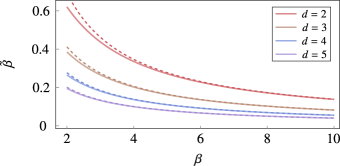
We present the comparison between our bound and the numerically obtained in Fig. 4. As can be observed, for large dimensions, the condition that needs to be much larger than one can be relaxed.
Appendix B Entanglement witnessing for Werner states
In this Appendix we specify the range of parameters for which the entanglement of Werner states can be certified using the witness from Sec. IV. For that we need to find the value for which the conditional entropy becomes negative. That is, the threshold value corresponds to the case when . This can be cast into the following transcendental equation:
| (57) |
The value which solves the above equation provides the boundary between negative and non-negative conditional entropy. The entanglement witness constructed in Sec. IV can witness Werner states for which .
Appendix C Entanglement witnessing for multipartite states
In this Appendix we discuuss how to extend our results from Sec. IV to multipartite states. Before we start, we recall a few mathematical relations that will be useful.
First, we write an expression for the von Neumann entropy of an -partite system in terms of a chain of conditional entropies. The starting point is to assume that the -partite system is bipartite , such that . By recursively applying this process times, we arrive at a general expression for the von Neumann entropy of a multipartite system as a chain of conditional entropies:
| (58) |
Second, we recall that the free energy of a (maximally) classically correlated system is given by:
| (59) |
where the second term is the mutual information, defined as . Consequently, expressing the joint entropy in terms of a chain of conditional entropies, we obtain that . Now, we write the mutual information in terms of the chain of conditional entropies as . Finally, putting together all this results, the free energy of the inital state is given by
| (60) |
Now, we notice that for separable states and that the largest free energy occurs when the chain of conditional entropies is zero. Futhermore, observe that the solution for the optimisation problem given by Eqs. (17)-(18) does not depend on whether is separable or not. Hence, its solution remains a thermal state at some inverse temperature . So, when we seek to optimize the heat exchange when is separable
| (61) | ||||
| (62) |
boils down to looking at the constraint. In this case, we know that the constraint is maximised (or the difference is maximised) when the chain of conditional entropies is zero, and this gives us the classical bound for the heat exchange.
As a final note, it is worth emphasizing that the condition can be directly inferred from the solution for , as seen in Eq. (6)]. However, the requirement for that the chain of conditional entropies must be zero may not be immediately apparent. This reveals a non-trivial relationship between the reduced entropies and the entropy of the output thermal state.