Renormalization, Decoupling and the Hierarchy Problem

Abstract

The hierarchy problem is associated with the renormalization and decoupling. By the decoupling of heavy fields, we can account for the smallness of the scalar mass against loop corrections and its insensitivity to ultraviolet physics. It is essential to correctly identify the observable parameters, which have natural convergence properties, as opposed to the bare ones. The loop corrections are finite and perturbatively expandable order by order. They are suppressed as powers of the external momentum to the mass ratio, according to the Appelquist–Carazzone decoupling theorem which we complete for the case of the scalar mass.

1 Introduction

In quantum field theory, a physical quantity is corrected by loop amplitudes. To the mass-squared parameter of a scalar field, e.g., the Higgs, loop corrections are added as

$$m_{B}^{2}+\sum_{\{l_{i}\}}\tilde{\Sigma}_{l_{1},l_{2},\dots,l_{n}}(p^{2}),$$ (1)

where $m_{B}^{2}$ is the bare mass-squared appearing in the Lagrangian and

$$\tilde{\Sigma}_{l_{1},l_{2},\dots,l_{n}}(p^{2})\propto\hbar^{l}g_{1}^{2l_{1}}g_{2}^{2l_{2}}\dots g_{n}^{2l_{n}}$$ (2)

are so-called the self-energy with the external momentum $p$ and the subscript denoting the dependence on the couplings $g_{1},g_{2},\dots g_{n}$ — the gauge, the Yukawa couplings and so on. We assume the amplitude is one-particle-irreducible thus $l=\lfloor\sum l_{i}\rfloor$, allowing half-integers $l_{i}$.

The scalar field theory suffers the hierarchy problem [1, 2, 3, 4, 5, 6, 7] (see also [9, 8, 10, 11, 12, 13]). It is well-known that each correction $\tilde{\Sigma}_{l_{1},l_{2},\dots,l_{n}}(p^{2})$ diverges quadratically, scaling as $\Lambda^{2}$, where $\Lambda$ is the momentum cutoff of the field in the loop. It is usually regarded as the scale up to which the effective theory is valid. This means the scalar mass is sensitive to unknown ultraviolet (UV) physics and needs to be well-defined in low energy. However, we shall see that this $\Lambda^{2}$ has little to do with the hierarchy problem. What is relevant are the other scaleful parameters, such as the mass $M$ of a field in UV physics, that also characterize the scale.

This paper points out that the hierarchy problem is related to renormalization and decoupling. By carefully following the renormalization procedure, we show that the heavy fields decouple and do not affect the scalar mass.

It is crucial to identify the observable physical parameters. Although the bare parameters define the theory, they can never be observed because the interactions modify them [1, 2]; hence, only the whole combination (1) can be observed. Thus, it is not necessary to make the loop corrections $\tilde{\Sigma}_{l_{1},l_{2},\dots,l_{n}}(p^{2})$ in (1) small, as attemped in the usual formulation. The common premise that $m_{B}^{2}$ is finite and small is not necessarily true, either. From the renormalization condition

$$m_{B}^{2}=m^{2}-\sum_{\{l_{i}\}}\tilde{\Sigma}_{l_{1},l_{2},\dots,l_{n}}(\mu^{2}),$$ (3)

where $m^{2}$ is the mass-squared indirectly observed at a renormalization point $p^{2}=\mu^{2}$, we see that, for small $m^{2}$, the other two should be comparable.

At first sight, the tuning between those two seems miraculous. However, the cancellation is natural. In effective field theory, the parameters in the Lagrangian quantify our ignorance and we fit them from the experiments. The one-parameter $m_{B}^{2}$ can be traded with the mass $m^{2}$ through the relation (3).

Using the relation (3), the Higgs mass admits well-defined perturbative expansion in terms of renormalized corrections

$$\begin{split}m^{2}(p^{2})&=m^{2}+\sum_{\{l_{i}\}}\delta m^{2}_{l_{1},l_{2},\dots,l_{n}}(p^{2})\\ &\equiv m^{2}+\sum_{\{l_{i}\}}(1-t_{\mu}^{2})\tilde{\Sigma}_{l_{1},l_{2},\dots,l_{n}}(p^{2}),\end{split}$$ (4)

where $t_{\mu}^{2}$ is the Taylor expansion operator up to two differentiation, in $p$ around the renormalization point. That is, the bare mass is the constant part of $m^{2}(p^{2})$ in (4).

It is shown by Zimmerman [15] that each term in the second line in (4) is finite. This means that each term is well-defined and finite even if we extend the momentum integral to infinite. This means the mass $m^{2}$ is independent of regularization or the cutoff $\Lambda$. There is no need for a miraculous cancellation. This should be finite because the same is obtained by running between the two scales, from $\mu$ to $p$, which is purely low-energy behavior [2]. If we wrote the Lagrangian using (3), there is no problem of infinity.

Our last concern is whether the Higgs mass depends on the UV parameters [16, 17, 18]. For instance, the scalar field can couple to a very heavy field with the mass $M$ and the loop correction can change the original scalar mass $m^{2}$. Then, the Appelquist–Carazzone decoupling theorem states that the corresponding amplitude is suppressed in some powers of $p^{2}/M^{2}$ and $m^{2}/M^{2}$ [19]. The renormalized loop corrections vanish as we send $M\to\infty$.

We show that this decoupling theorem also holds for the scalar mass. That is, the effect on a UV field vanishes in the limit of its heavy mass [1, 2]

$$\quad M\to\infty\quad\Longrightarrow\quad\delta m^{2}_{l_{1},l_{2},\dots,l_{n}}(p^{2})\to 0,$$ (5)

if this particular mass correction involves the field of the heavy mass $M$. This justifies the claim that there is no dependence on the UV physics in the scalar mass.

2 On-shell renormalization using counterterms

We briefly review the conventional renormalization using counterterms. We are mainly interested in an example of the $\phi^{4}$-theory, which appears as the Higgs sector in the Standard Model. The Lagrangian density is

$${\cal L}=\frac{1}{2}\partial_{\mu}\phi\partial^{\mu}\phi-\frac{1}{2}m_{B}^{2}\phi^{2}-\frac{6\lambda_{B}}{24}\phi^{4}.$$ (6)

The mass $m_{B}^{2}$ and the quartic coupling $\lambda_{B}$ are bare parameters defining the theory.

If we calculate the actual scattering amplitude, quantum corrections modify the observed parameters. Such corrections typically diverge, which is to be remedied as follows.

We re-normalize the field

$$\phi=\sqrt{Z}\phi_{r}$$ (7)

to rewrite the Lagrangian (6)

$$\begin{split}{\cal L}&=\frac{1}{2}\partial_{\mu}\phi_{r}\partial^{\mu}\phi_{r}-\frac{1}{2}m^{2}\phi_{r}^{2}-\frac{6\lambda}{24}\phi_{r}^{4}+\frac{1}{2}\delta_{Z}\partial_{\mu}\phi_{r}\partial^{\mu}\phi_{r}-\frac{1}{2}\delta_{m}\phi_{r}^{2}-\frac{6\delta_{\lambda}}{24}\phi_{r}^{4}.\end{split}$$ (8)

If we instead newly introduce counterterms on top of the bare Lagrangian, we redefine the theory.

In the on-shell (OS) or physical scheme (see, e.g.,[20, 21]), we regard the parameters $m^{2}$ and $\lambda$ as the observed ones through the scattering process at a reference scale, to be discussed below. The (Feynman) propagator contains the mass $m^{2},$

$$D(p^{2})=\frac{i}{p^{2}-m^{2}},$$ (9)

and treat the remaining terms, so-called counterterms, of

$$\delta_{Z}=Z-1,\quad\delta_{m}=m_{B}^{2}Z-m^{2},\quad\delta_{\lambda}=\lambda_{B}Z^{2}-\lambda$$ (10)

as perturbative interactions. They are going to absorb the divergences from the loop amplitude. Due to the symmetric factor and normalization in (8), the good expansion parameter is $6\lambda$ and $6\delta_{\lambda}$ in this paper.

In quantum theory, it is always modified by the self-energy $-i\tilde{\Sigma}(p^{2})$, the total 1PI amplitude with two external legs. The leading correction comes from the one-loop

$$-i\tilde{\Sigma}_{1}(p^{2})=\frac{1}{2}\int\frac{d^{4}k}{(2\pi)^{4}}(-6i\lambda)D(k^{2}).$$ (11)

Likewise, we have higher-order corrections $\tilde{\Sigma}_{l}(p^{2}).$

To remove the divergence, we impose a renormalization condition that the mass used in the propagator remains the same, to ${\cal O}(p^{2}-m^{2})$. That is, the quantum correction to the propagator should be

$$\left[\tilde{\Sigma}(p^{2})+6p^{2}\delta_{Z}-6\delta_{m}\right]_{p^{2}=m^{2}}=0,$$ (12)

to all orders of perturbation. We are free to choose expansion parameters and their reference points. From dimensional analysis, the self-energy $\tilde{\Sigma}(p^{2})$ is quadratic polynomial in $\sqrt{p^{2}}$. The constant $\delta_{m}$ is always chosen to keep the total mass at the specific value at $p^{2}=m^{2}$ unchanged. At the same time, it takes away the quadratic divergence in $\tilde{\Sigma}(p^{2})$. Our theory has parity symmetry, so there is no linear term for $p$. The constant $\delta_{Z}$ absorbs the logarithmic divergence in the coefficient of $p^{2}$ in $\tilde{\Sigma}(p^{2})$.

We regard the interaction as a small perturbation and calculate loop corrections order by order; further corrections may also modify the observed parameters. Thus, we regard that the parameters in the counterterms are to be expanded in powers of $\hbar$, which is equal to the number of loops

$$\delta_{Z}=\sum_{l=1}^{\infty}\hbar^{l}\delta_{Zl},\quad\delta_{m}=\sum_{l=1}^{\infty}\hbar^{l}\delta_{ml},\quad\delta_{\lambda}=\sum_{l=1}^{\infty}\hbar^{l}\delta_{\lambda l}.$$ (13)

At each loop order $l$, the condition (12) means, to the accuracy ${\cal O}(\hbar^{l+1}\lambda^{2l+2})$,

$$\quad 6\delta_{ml}=\tilde{\Sigma}_{l}(m^{2}),\quad 6\delta_{Zl}=-\frac{d\tilde{\Sigma}_{l}}{dp^{2}}(m^{2}).$$ (14)

After calculating a physical parameter to ${\cal O}(\lambda^{n})$, we impose the renormalization condition as the vanishing corrections and the physical parameter does not change. Further ${\cal O}(\hbar^{L+1})$ corrections may diverge, which must be absorbed by the counterterm of the same order, having the same divergence. Nevertheless, we hope that the canceled combination will be small enough ${\cal O}(\lambda^{n+1})$ to neglect it.

What is the prediction if all the quantum corrections to the propagator do not modify the observed mass by default? We have fixed the counterterm in the specific form as in (14). The quadratic interaction generally changes due to loop corrections $\tilde{\Sigma}_{n}(p^{2})$ and becomes a function of the external momentum $p^{2}$. In other words, the following effective interactions are induced in the momentum space

$$\delta{\cal L}=\sum_{l=1}^{\infty}\frac{1}{2}\left[-\tilde{\Sigma}_{l}(m^{2})+(p^{2}-m^{2})\frac{d\tilde{\Sigma}_{l}}{d(p^{2})}(m^{2})\right]\phi_{r}^{2},$$ (15)

in addition to the mass term. The momentum-dependent part is the only observational consequence of the loop-corrections. We cannot detect the constant shift in the quadratic interaction by construction in the OS scheme, as expressed in (12). In another scheme, we may take a different reference $m^{2}$ (indirectly through the propagator) and measure the departure of the mass $m^{2}(p^{2})$ from it. If we were to take the reference mass differently, additional loop corrections plus the corresponding counterterms would make the prediction for the mass more precise. A good and timely example is the Higgs mass profile from the dominant one-loop correction due to the top quark [1, 2].

3 Renormalization without counterterms

We have another way to achieve renormalization without introducing counterterms. The free particle is described by the propagator

$$D^{B}(p^{2})=\frac{i}{p^{2}-m_{B}^{2}},$$ (16)

encoding the information on the bare mass. It receives quantum corrections by the 1PI self-energy $-i\tilde{\Sigma}(p^{2})$. Collecting all the reducible diagrams, we have the geometric sum

$$\begin{split}D^{\prime}(p^{2})&=D^{B}(p^{2})+D^{B}(p^{2})[-i\tilde{\Sigma}(p^{2})]D^{B}(p^{2})+\dots\\ &=\frac{i}{p^{2}-m_{B}^{2}}\frac{1}{1+i\tilde{\Sigma}(p^{2})\frac{i}{p^{2}-m_{B}^{2}}}\\ &=\frac{i}{p^{2}-m_{B}^{2}-\tilde{\Sigma}(p^{2})}.\end{split}$$ (17)

The mass, to be probed by scattering experiments with this propagator, is changed. We take a reference mass for the expansion as the pole mass $m$ defined as

$$\left[p^{2}-m_{B}^{2}-\tilde{\Sigma}(p^{2})\right]_{p^{2}=m^{2}}=0.$$ (18)

At this pole, the residue of the propagator is changed, which comes from the next leading order expansion from $\tilde{\Sigma}(p^{2})$ from the reference mass

$$p^{2}\to m^{2}:\frac{i}{p^{2}-m_{B}^{2}-\tilde{\Sigma}(p^{2})}\to\frac{iZ}{p^{2}-m^{2}}+{\cal O}((p^{2}-m^{2})^{2}).$$ (19)

We renormalize the field as in (7), with the field strength $Z$ being

$$Z^{-1}=1-\frac{d\tilde{\Sigma}}{dp^{2}}(m^{2}).$$ (20)

The resulting propagator is the same as that in (9) to ${\cal O}(p^{2}-m^{2}),$ justifying its use. Therefore, we calculate the amplitude, including $\tilde{\Sigma}(p^{2})$, using the physical mass $m$.

A scattering amplitude with the momentum $p^{2}$ will be described by the propagator (17). From the denominator in the propagator (19), we are naturally led to define the momentum-dependent “running mass”

$$m^{2}(p^{2})\equiv m_{B}^{2}+\tilde{\Sigma}(p^{2})-(p^{2}-m^{2})\frac{d\tilde{\Sigma}}{dp^{2}}(m^{2}).$$ (21)

Using the pole mass, (18), we can eliminate the bare mass,

$$m^{2}(p^{2})=m^{2}+\tilde{\Sigma}(p^{2})-\tilde{\Sigma}(m^{2})-(p^{2}-m^{2})\frac{d\tilde{\Sigma}}{dp^{2}}(m^{2}).$$ (22)

In the RHS, the first $m^{2}$ and the sum of the rest terms are separately finite and independent of regularization, as seen in the next section.

The bare parameter is not observable and we may choose not to use it in the renormalization. What is important is the whole combination, or the running mass (22), which can be defined without reference to the bare parameter.

Of course, this description is equivalent to the previous one with counterterms if we absorb the counterterms for $\delta_{M},\delta_{Z}$ in the mass and the propagator, not treating them as perturbative interactions. There is a one-to-one correspondence between the loop correction and the counterterm as in (14). Although equivalent, the renormalization in this section did not care about the divergence of the loop amplitudes.

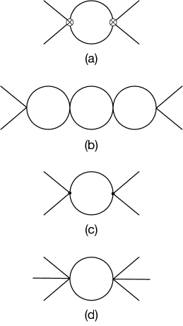
Figure 1: Neither loop-correction nor counterterm is not separately observable but only the combination is. (a) The one-loop diagram involving the counterterm coupling $\delta_{\lambda}$ (denoted by crossed circles). The corresponding amplitude is divergent. A counter-counterterm to this may give rise to another new divergence. (b) The only way to cancel this kind of divergence is to have special combination with ordinary loop diagrams with physical couplings. (c) If we always have the combination of the renormalized physical couplings (denoted by big dots), there is no additional divergence. (d) There is no problem in the cancellation of divergence for irrelevant operators.

We remark on what the conventional counterterm approach may need to be addressed. Since the counterterms provide interactions, we are tempted to take into account all the possible loop corrections with them. It can also give rise to divergences, for example, from the amplitude in Fig. 1 (a). Then, we worry that we need a quartic counter-counterterm to cancel the additional divergence. This gives rise to proliferating counterterms, which is the criterion for non-renormalizability.

However, this always happens in the renormalizable theory. This means only a particular combination can cancel the divergence from the counterterms. The amplitude for Fig. 1 (a) can be canceled by the physical loop in Fig. 1 (b). These two diagrams correspond to parts of the (subdiagram-)renormalized amplitude Fig. 1 (c)

$$\int d^{4}k_{1}d^{4}k_{2}d^{4}k_{3}[V(p+k_{1})-V(\mu)]V(p+k_{2})[V(p+k_{3})-V(\mu)],$$ (23)

where

$$iV(p^{2})\equiv\frac{1}{2}\int\frac{d^{4}k}{(2\pi)^{4}}D(k)D(k+p)$$ (24)

is the one-loop corrected vertex and we identified the counterterm $\delta_{\lambda 1}\sim V(\mu)$. The renormalized subdiagram is denoted by big dots in Fig. 1 (c).

It is more evident from the natural subtracted pair; if we have the amplitude Fig. 1 (b), we always have Fig. 1 (a) and vice versa; whenever we have a counterterm parameter in the amplitude, we have an amplitude with this counterterm replaced with loop sub-amplitude. This amplitude is again part of the completely renormalized three-loop quartic coupling

$$\int d^{4}k_{1}d^{4}k_{2}d^{4}k_{3}[V(p+k_{1})-V(\mu)][V(p+k_{2})-V(\mu)][V(p+k_{3})-V(\mu)].$$ (25)

(Of course, there are other diagrams, but this is one finite component.) This also means that the counterterm parameters are not the observables, which is equivalent to saying that the bare parameters are not the observables.

The above structure is always there, and the cancellation of small-scale physics is a bonus. The essence of renormalization is to reveal the scale dependence of the physical parameter, not the cancellation of divergence. Although fixing the physical mass itself does not give a prediction, the scale-dependence correction to the mass is a prediction.

Finally, we usually say that a non-renormalizable interaction is not renormalizable because we need infinitely many counterterms to absorb the divergence. For instance, a $\phi^{5}$ interaction generates an effective one as in Fig. 1 (d), which is effectively $\phi^{6}$ interaction requiring as many counterterms. Because of the natural pairing, we have indeed as many counterterms. The problem with non-renormalizable theory is that it may not admit effective interactions like higher-derivative couplings. ‘

4 Regularization scheme independence

We discuss the cancellation of the divergence in more detail.

Loop corrections are divergent because the loop integration extends to an arbitrary high-momentum scale. This is the limit of our only available calculational tool, the Lorentz-covariant continuum field theory. Conceptually, if the self-energy $\tilde{\Sigma}(p^{2})$ diverges as in (18), if the mass $m^{2}(p^{2})$ that we observe is finite, then the bare mass $m_{B}^{2}$ must similarly diverge.

Usually, we crystalize the infinity as a limit of a parameter $\Lambda$ by regularization. Again, we note that the physical quantity after renormalization is expressed as the difference between the same quantities at different scales. There is natural cancellation and, ultimately, they are expected to be finite or insensitive to $\Lambda$ [1].

In the simplest example of the one-loop correction to the scalar mass, we have

$$\int\frac{d^{4}k}{(2\pi)^{4}}\left[\frac{1}{\left(k^{2}-\Delta\right)^{2}}-\frac{1}{\left(k^{2}-\Delta^{\prime}\right)^{2}}\right]=\frac{i}{16\pi^{2}}\log\frac{\Delta^{\prime}}{\Delta}.$$ (26)

We obtain the same answer if we perform the integral separately by introducing momentum cutoff, doing dimensional regularization [32, 33] or Pauli–Villars regularization. The same holds true for the one-loop vacuum polarization and the scalar mass [1].

This natural cancellation behavior is rephrased as in the BPHZ scheme [23, 24, 25, 15, 26, 27] (see also [29, 28]). The renormalized quantity $Q(p^{2})$ is defined

$$Q(p^{2})=Q_{B}+\int I=Q_{\text{phy}}+(1-t^{D})\int I,$$ (27)

where $D$ is the superficial degree of divergence [14]. The integration for the Feynman diagram is done over the loop momenta. The above removes, assuming that possible subdiagram divergences are canceled by BPHZ prescription [23, 24, 25, 15, 26, 27].

In four dimensions, the scalar mass-squared (31) has $D=2$ and contains quadratic divergence. Thus,

$$m^{2}(p^{2})=m^{2}+\sum_{\{l_{i}\}}(1-t_{m}^{2})\tilde{\Sigma}_{l_{1},l_{2},\dots,l_{n}}(p^{2}).$$ (28)

For (super-)renormalizable quantity, we may always go to Wick rotated space to show the convergence and use the Feynman prescription [15].

We may even use the subtracted integrand, whose leading power cancels and has a lower power in the momentum. Thus, BPHZ uses the finite quantity

$$Q(p^{2})=Q_{\text{phy}}+\int(1-t^{D})I,$$ (29)

which is scheme-independent by default (if the exchange is permissible). Suppose we do not deal with the individual quantity in the subtract pair. In that case, we do not need to introduce unrealistic auxiliary theory like fields with wrong spin-statistics or heavy gauge bosons.

Therefore, specifying the renormalization condition at an agreed scale completely specifies the physical parameters. Since this is the only observable combination, it is natural to define this as the running physical quartic coupling. It is independent of the regularization scheme in the above sense. In this paper, running physical parameters are scale-dependent.

From the above, we see that the momentum cutoff $\Lambda$ in the integral has nothing to do with the hierarchy. Evidently, the loop correction by a massless field introduces no scale, providing an example that $\Lambda$ is not related. What we require is that the physical quantities we calculate have sufficiently close asymptotic behavior so that, for instance, for the self-energy $\tilde{\Sigma}(p^{2})$ is close to $\tilde{\Sigma}(m^{2})$ to the accuracy ${\cal O}(p^{2}/\Lambda^{2})$ [1]. Due to the natural pair-subtraction property, sufficient high-momentum contributions cancel and $\Lambda$ does not appear in the (super-)renormalizable parameters. In fact, the parameter $\Lambda$ is human-made, which is overlooked in the Wilsonian renormalization [2, 21] by a dimensionful parameter, e.g., the mass $M$, of the fields involved in the loop, provided by Nature.

In the above example, the effective mass $m^{2}(p^{2})$, in the end, is given by the solution to the renormalization-group equation with the initial condition set at a reference scale, $m^{2}$. Therefore this quantity does not see the high-scale contribution. The Wilsonian approach more clearly shows this [2].

5 The Hierarchy Problem

Now, we discuss the hierarchy problem. If one regards the bare mass $m_{B}^{2}$ in (21) as “God-given” from the beginning,

$$m^{2}(p^{2})=m_{B}^{2}+\sum_{\{l_{i}\}}\left[\tilde{\Sigma}_{l_{1},l_{2},\dots,l_{n}}(p^{2})-(p^{2}-m^{2})\frac{d\tilde{\Sigma}_{l_{1},l_{2},\dots,l_{n}}}{dp^{2}}(m^{2})\right],$$ (30)

using the notation in (2), it seems miraculous to have the rest of the corrections canceled to perfect accuracy to yield the observed small mass. There is, in general, more than one coupling, so some coupling we have yet to consider would also ruin the finite mass. In the Standard Model, we have corrections involving three gauge couplings and Yukawa couplings, in addition to the quartic self-coupling. Every loop correction from them has divergence. So, we need more delicate relations between counterterms.

Traditionally, the hierarchy problem has been why the correction $\tilde{\Sigma}(p^{2})$ is small, assuming small $m_{B}^{2}$ for some reason. Its understanding is guided by the naturalness criterion of ’t Hooft [30]. If we make the parameter (here, the bare mass) zero, there is emerging symmetry forbidding this parameter. This means the loop corrections are proportional to the original coupling by this symmetry, or the renormalization is multiplicative. This explains the smallness of the whole parameter; if we have some reason to have a small original parameter, all the corrections are proportional to it and the total coupling becomes parametrically small. Known examples are gauge symmetry and chiral symmetry. It is well-known that scalar mass renormalization is not protected by symmetry and is not multiplicative.

However, the renormalization condition (18) suggests that $m_{B}^{2}$ should be big around the UV scale. Then, the required cancellation becomes more unnatural because there should be a cancellation between $m_{B}^{2}$ and all the $\tilde{\Sigma}_{l_{1},l_{2},\dots,l_{n}}$’s to fine-tune the mass. A technical hierarchy problem arises once we force the quantum-corrected mass to be finite (presumably the observable value) at a given order $g_{1}^{L_{1}}g_{2}^{L_{2}}\dots g_{n}^{L_{n}}$, always higher order correction ruins the smallness, making the sum divergent. There needs to be a miraculous cancellation in any case.

We emphasize that we do not need to explain the smallness of the $\tilde{\Sigma}(p^{2})$ part. Because this and the bare parameters are never separable; what needs to be small is the combination [1].

Remember that our theory is the effective field theory, and the parameter $m_{B}^{2}$ in the Lagrangian is just parametrizations of our ignorance but valid below a certain scale and is to be matched with the counterpart in the UV completion or simply the observables (see e.g. [17, 37, 38]). We have another equivalent but better alternative one-parameter parametrization $m^{2}$, seen in Eq. (22). Using the relation, the running physical mass (30) is expressed as

$$\begin{split}m^{2}(p^{2})&=m^{2}+\sum_{\{l_{i}\}}\left[\tilde{\Sigma}_{l_{1},l_{2},\dots,l_{n}}(p^{2})-\tilde{\Sigma}_{l_{1},l_{2},\dots,l_{n}}(m^{2})-(p^{2}-m^{2})\frac{d\tilde{\Sigma}_{l_{1},l_{2},\dots,l_{n}}}{dp^{2}}(m^{2})\right]\\ &\equiv m^{2}+\sum_{\{l_{i}\}}(1-t_{m}^{2})\tilde{\Sigma}_{l_{1},l_{2},\dots,l_{n}}(p).\end{split}$$ (31)

Since the mass always appears in this combination, the cancellation of divergence is built-in. We understand why the loop corrections are canceled to be finite order by order. Each term in the square bracket is finite and small; it is interpreted as the perturbative expansion of the mass giving the relation (4), is small, in coupling $g_{1},g_{2},\dots g_{n}$ in $l$-loop. As long as there is no convergence problem, it is not difficult to convince ourselves that each correction becomes smaller and the perturbation works. Higher-order terms and/or loops in different couplings are parametrically small, and we can approximate and calculate them to the desired accuracy. We need Dirac’s naturalness: all the parameters appearing in the loop correction are of order one [36].

Although the bare parameter defines the effective theory, it is not observable. What is observable is the running mass (22), which can be determined without the reference to the bare parameter. It is desirable to remove unobservable bare parameters. That is, we may alternatively define the theory using the physical mass $m$ that is measurable, then the bare mass is derived from the relation (18),

$$m_{B}^{2}=m^{2}-\tilde{\Sigma}(m^{2}).$$ (32)

Once we fix $m^{2}$, calculating higher-order loop corrections makes the bare mass more precise. Conversely, if we regard the bare mass $m_{B}^{2}$ fixed, the calculation more precisely corrects the (constant part) of the physical parameter. The difference can also be understood as fixing the counterterms. This also justifies the expansion (13) through the identification of the counterterms using (31).

The original formulation by Gildener essentially addressed a technical hierarchy problem concerning stability with respect to higher-order loop corrections discussed in this paper [3, 4]. In the Grand Unified Theory, however this problem is tightly related to the hierarchy of scales. In the original formulation, the minimization condition for the scalar field, required for breaking the unified group like $SU(5)$ down to the Standard Model group, should satisfy the hierarchical relation, however, loop corrections generically ruin it.

In modern understanding, we can separate the symmetry-breaking source for the GUT and Standard Model groups. In string-theory-based construction, the former is broken by instantons in the extra dimensions and the latter by the Higgs scalar (see e. g. [31]), which are not a priori dependent.

In this paper, we do not deal with the “big” hierarchy problem, which is why the electroweak scale is way much smaller than the fundamental, the Planck scale.

6 Decoupling in the scalar mass

Finally, we propose that decoupling solves the technical hierarchy problem. So far, we have seen that the loop corrections are perturbative and divergence-free. It remains to be shown that any of them involved in a heavy field are suppressed.

The Appelquist–Carazzone decoupling theorem states that a 1PI amplitude involving a heavy field in the loop is suppressed as some powers of $p^{2}/M^{2}$ [19]. The sketch of the proof goes as follows. A loop diagram with $n$ external bosons with momentum $\sim\sqrt{p^{2}}$ scales like $p^{4-n}$. Considering a subdiagram in the loop diagram with the internal propagator of the field with the mass $M$, the subdiagram amplitude behaves like $M^{f-n}$ in the heavy mass limit. This subdiagram shrinks and becomes $(f-n)$-point amplitude. The total amplitude behaves like $M^{4-f}M^{f-n}=M^{4-n}$. It has shown that the heavy fields decouple in the strictly renormalizable (marginal) quantity. This means we do not need to care about heavy fields in the low energy limit.

One technical gap is a possible exception of the scalar mass-squared parameter. Although the original proof assumes external photons whose quadratic divergence is not taken care of, the case for the scalar propagator gives essentially the same result. We complete it.

Let us suppose that there are super-heavy scalar $X$ and Dirac field $\psi$ at the UV, described by the interaction

$$-\frac{1}{2}M_{s}^{2}X^{2}-\kappa\phi^{2}X^{2}-M_{f}\overline{\psi}\psi-y\phi\overline{\psi}\psi+\dots$$ (33)

The UV scale is characterized by $M_{s},M_{f}$. The decoupling limit is $M_{s},M_{f}\to\infty$ or $M_{s}^{2},M_{f}^{2}\gg m^{2},p^{2}$ to be precise.

The general form of $n$-loop amplitude as (we denote one index for simplicity, but the multi-coupling generation is straightforward)

$$\tilde{\Sigma}_{n}(p^{2})=\int d^{4}k_{1}\dots d^{4}k_{n}P(p,k_{1},\dots,k_{n})\prod_{j}\frac{1}{L_{j}(p,k_{1},\dots,k_{n})-m_{j}^{2}},$$ (34)

where $L_{j}$ is a quadratic function of the momenta and $P$ is a polynomial arising from the spin of the fields. Using the Feynman parameterization

$$\tilde{\Sigma}_{n}(p^{2})=\int d{\bf x}\int d^{4}k_{1}\dots d^{4}k_{n}\frac{\tilde{P}(k_{1},\dots,k_{n})}{[Q(p,k_{1},\dots,k_{n})+\Delta_{n}]^{n}}$$ (35)

with the collective notation ${d\bf x}=dx_{1}\dots dx_{n}$ allowing some monomial factors $x_{i}^{k}$. $\tilde{P}$ is another polynomial and $Q$ a is a quadratic function in $k_{i}$, whose details are not important here. By completing the square in every $k_{i}$, we can always single out the dependence in $p^{2}$ and $M^{2}$ into the unique combination

$$\Delta_{n}=-f_{n}({\bf x})p^{2}+\sum g_{i}(x_{i})m_{i}^{2},$$

where $f({\bf x}),g_{i}(x_{i})$ are the coefficients of $p^{2},m_{i}^{2},$ respectively. We imagine that some of the mass are those of heavy fields in (33). It is convenient to introduce the average mass $M$

$$g_{n}({\bf x})M^{2}=\sum g_{i}(x_{i})m_{i}^{2},$$ (36)

with some coefficient $g_{n}({\bf x})$. In the decoupling limit, we thus have $M^{2}\gg m^{2},p^{2}$.

Since $\tilde{\Sigma}_{n}(p^{2})$ is mass dimension two and is a function of $\Delta_{n}$ that is also dimension two. After the momentum integration and cancellation of subdiagram divergence a la BPHZ, dimensional analysis suggests the amplitude has the form

$$\tilde{\Sigma}_{n}(p^{2})=\int d{\bf x}\left[A_{n}+c_{n}\Delta+(d_{n}+e_{n}\Delta_{n})\log\frac{B_{n}}{\Delta_{n}}\right],$$ (37)

for each $n$, where $c_{n},e_{n}$ are order-one constants. Also, $d_{n}$ is a constant of mass dimension two, independent of heavy fields, or $d_{n}\ll M$. The divergence is regularized as a $p^{2}$-independent constants $A_{n}$ and $B_{n}$, both of which are mass dimension two. The physical mass is

$$\begin{split}m^{2}(p^{2})&=m^{2}+\sum_{n}\left\{\tilde{\Sigma}_{n}(p^{2})-\tilde{\Sigma}_{n}(m^{2})-(p^{2}-m^{2})\frac{d\tilde{\Sigma}_{n}}{dp^{2}}(m^{2})\right\}\\ &=m^{2}+\sum_{n}\left\{\int d{\bf x}\left[(d_{n}+e_{n}\Delta_{n})\log\frac{\Delta_{n}}{\Delta_{n}^{\prime}}+\frac{d+e\Delta_{n}^{\prime}}{\Delta_{n}^{\prime}}f({\bf x})(p^{2}-m^{2})\right]\right\},\end{split}$$ (38)

where we define $\Delta^{\prime}_{n}\equiv-f_{n}({\bf x})m^{2}+g_{n}({\bf x})M^{2}.$ The quadratic divergence $A_{n}$ is cancelled in $\tilde{\Sigma}_{n}(p^{2})-\tilde{\Sigma}_{n}(m^{2})$ and the logarithmic divergence $B_{n}$ is cancelled in the first order Taylor expansion in $p^{2}$ [1].

Now, in the decoupling limit $M\to\infty$, we have $d_{n}\ll e_{n}\Delta_{n}$ and $\Delta_{n}\to g_{n}M^{2}(1-f_{n}p^{2}/M^{2}+\dots)$, so that, for each $n$,

$$\begin{split}\delta m_{n}^{2}(p^{2})&=\int d{\bf x}\left[eM^{2}\left(\frac{f_{n}p^{2}}{M^{2}}+\frac{f_{n}^{2}p^{4}}{2M^{4}}+{\cal O}\left(\frac{p^{6}}{M^{6}}\right)-\frac{f_{n}m^{2}}{M^{2}}-\frac{f_{n}^{2}m^{4}}{2M^{4}}-{\cal O}\left(\frac{m^{6}}{M^{6}}\right)\right)\right.\\ &\qquad-e_{n}f_{n}(p^{2}-m^{2})\bigg{]}\bigg{\}}\\ &=e_{n}\int d{\bf x}\left[\frac{f_{n}^{2}p^{4}}{2M^{2}}-\frac{f_{n}^{2}m^{4}}{2M^{2}}+{\cal O}\left(\frac{p^{6}}{M^{4}}\right)-{\cal O}\left(\frac{m^{6}}{M^{4}}\right)\right].\end{split}$$ (39)

The cancellation of the quadratic terms takes place. Naively, the loop correction is proportional to $M^{2}\log M^{2}$. However, in the physical mass, the leading order contributions cancel and the total amplitude is suppressed as

$$\frac{p^{4}}{M^{2}}\text{\quad and \quad}\frac{m^{4}}{M^{2}}.$$ (40)

In the heavy mass limit, the corresponding mass correction vanishes

$$M\to\infty\quad\Longrightarrow\quad\delta m_{n}^{2}(p^{2})\to 0.$$ (41)

This is the suppression expected by the Applequist–Carazzone decoupling theorem, which we extend for the case with two external bosons. We expect a similar decoupling behavior in the super-renormalizable operators. It exhibits power running, seen from the dependence in $p^{2}$ [2]. Light fields can correct the mass sizably, but they are not hierarchical.

For reference, we verify this for the one-loop contribution from a fermion in (33)

$$\begin{split}-i\tilde{\Sigma}_{y}(p^{2})&=-2y^{2}\int_{0}^{1}dx\int\frac{d^{4}\ell}{(2\pi)^{4}}\frac{\ell^{2}-x(1-x)p^{2}-M_{f}^{2}}{(\ell^{2}+x(1-x)p^{2}-M_{f}^{2})^{2}}\\ &=\frac{2y^{2}}{16\pi^{2}}\int_{0}^{1}dx\left[\Lambda^{2}-2(M_{f}^{2}-x(1-x)p^{2})\log\frac{\Lambda^{2}}{M_{f}^{2}-x(1-x)p^{2}}-M_{f}^{2}+x(1-x)p^{2}\right],\end{split}$$ (42)

where we introduced a simple momentum cutoff $\Lambda$. This is of the same form as (37) with $f(x)=x(1-x),g(x)=1,b=-1,c=0,e=-2$. Although it diverges, the combination $\tilde{\Sigma}_{y}(p^{2})-\tilde{\Sigma}_{y}(M_{f}^{2})$ and hence the running physical mass $m^{2}(p^{2})$ in (39) converge. It vanishes in the limit $M_{f}\to 0.$

Another example is a two-loop contribution including a heavy scalar $X$. We have two amplitudes

$$\tilde{\Sigma}_{\lambda,\kappa,1}(p)=S_{1}\int\frac{d^{4}l}{(2\pi)^{4}}(-i\lambda)^{2}V_{M_{s}}(p+l)\frac{i}{l^{2}-m^{2}},$$ (43)

$$\tilde{\Sigma}_{\lambda,\kappa,2}(p)=S_{2}\int\frac{d^{4}l}{(2\pi)^{4}}(-i\lambda)^{2}V_{m}(p+l)\frac{i}{l^{2}-M^{2}},$$ (44)

where $V_{M}(p)$ is the one-loop corrected vertex (24) with the mass of the internal scalar $M$ and $S_{1},S_{2}$ are appropriate symmetry factor. Here, $\tilde{\Sigma}_{\lambda,\kappa,1}(p)$ vanishes because $V_{M_{s}}(p+l)-V_{M_{s}}(\mu)$ reduces to the physical one due to decoupling of $X$ after the renormalization of subamplitude. Then, the overall amplitude is essentially the one-loop, which vanishes as stated. The nontrivial one is the second one that is evaluated as

$$\begin{split}\tilde{\Sigma}(p)_{\lambda,\kappa,2}=-S_{2}(i\lambda)^{2}\frac{-i}{2}\int&\frac{d^{4}l}{(2\pi)^{4}}\int dxdy\frac{\Gamma(3-\frac{d}{2})}{(4\pi)^{d/2}}y^{1-d/2}\\ \times&\frac{1}{[ym^{2}-yx(1-x)(p+l)^{2}+(1-y)(l^{2}-M_{s}^{2})]^{3-d/2}}.\end{split}$$ (45)

This time, we employed dimensional regularization [39]. It is not difficult to perform the $l$-momentum integral; we are content with showing the decoupling in the large $M$ limit. In this case, the denominator in the last factor can be approximated as

$$[1-y-yx(1-x)]l^{2}+(1-y)M_{s}^{2},$$ (46)

so that

$$\tilde{\Sigma}_{\lambda,\kappa,2}(p)=-S_{2}\lambda^{2}\frac{1}{2(4\pi)^{d}}\frac{\Gamma(3-d)}{\Gamma(3-\frac{d}{2})}\int dxdy(-y)^{1-d/2}\frac{1}{M_{s}^{3-d}}.$$ (47)

Therefore, the difference vanishes, and the heavy scalar field $X$ decouples in the scalar mass correction.

In summary, the scalar mass is not sensitive to UV physics because the correction of the heavy field is suppressed. Also, the renormalized physical quantity is scheme-independent. Correct identification of physical observables is essential.

Acknowledgments

The author thanks Jong-Hyun Baek, Sungwoo Hong, Hyung-Do Kim, Bumseok Kyae, Lisa Im, Stefan Groot Nibbelink, Hans-Peter Nilles, Ruiwen Ouyang, Mu-In Park, Jaewon Song and Piljin Yi for discussions. This work is partly supported by the grant RS-2023-00277184 of the National Research Foundation of Korea.

References

- [1] K.-S. Choi, “On the observables of renormalizable interactions,” J. Korean Phys. Soc. 84 (2024) no.8, 591-595 doi:10.1007/s40042-024-01025-7 [arXiv:2310.00586 [hep-ph]].
- [2] K.-S. Choi, “Exact renormalization of the Higgs field,” Phys. Rev. D 109 (2024) no.7, 076008 doi:10.1103/PhysRevD.109.076008 [arXiv:2310.10004 [hep-th]].
- [3] E. Gildener, “Gauge Symmetry Hierarchies,” Phys. Rev. D 14 (1976), 1667 doi:10.1103/PhysRevD.14.1667
- [4] E. Gildener, “GAUGE SYMMETRY HIERARCHIES REVISITED,” Phys. Lett. B 92 (1980), 111-114 doi:10.1016/0370-2693(80)90316-0
- [5] S. Weinberg, “Gauge Hierarchies,” Phys. Lett. B 82 (1979), 387-391 doi:10.1016/0370-2693(79)90248-X
- [6] A. A. Natale and R. C. Shellard, “THE GAUGE HIERARCHY PROBLEM,” J. Phys. G 8 (1982), 635 doi:10.1088/0305-4616/8/5/005
- [7] L. Susskind, “THE GAUGE HIERARCHY PROBLEM, TECHNICOLOR, SUPERSYMMETRY, AND ALL THAT.,” Phys. Rept. 104 (1984), 181-193 doi:10.1016/0370-1573(84)90208-4
- [8] Y. Hamada, H. Kawai and K. y. Oda, Phys. Rev. D 87 (2013) no.5, 053009 [erratum: Phys. Rev. D 89 (2014) no.5, 059901] doi:10.1103/PhysRevD.87.053009 [arXiv:1210.2538 [hep-ph]].
- [9] M. Farina, D. Pappadopulo and A. Strumia, JHEP 08 (2013), 022 doi:10.1007/JHEP08(2013)022 [arXiv:1303.7244 [hep-ph]].
- [10] J. D. Wells, “The Utility of Naturalness, and how its Application to Quantum Electrodynamics envisages the Standard Model and Higgs Boson,” Stud. Hist. Phil. Sci. B 49 (2015), 102-108 doi:10.1016/j.shpsb.2015.01.002 [arXiv:1305.3434 [hep-ph]].
- [11] A. Hebecker, “Lectures on Naturalness, String Landscape and Multiverse,” [arXiv:2008.10625 [hep-th]].
- [12] N. Craig and S. Koren, “IR Dynamics from UV Divergences: UV/IR Mixing, NCFT, and the Hierarchy Problem,” JHEP 03 (2020), 037 doi:10.1007/JHEP03(2020)037 [arXiv:1909.01365 [hep-ph]].
- [13] S. Mooij and M. Shaposhnikov, “QFT without infinities and hierarchy problem,” Nucl. Phys. B 990 (2023), 116172 doi:10.1016/j.nuclphysb.2023.116172 [arXiv:2110.05175 [hep-th]].
- [14] S. Weinberg, “High-energy behavior in quantum field theory,” Phys. Rev. 118, 838-849 (1960) doi:10.1103/PhysRev.118.838;
- [15] W. Zimmermann, “Convergence of Bogolyubov’s method of renormalization in momentum space,” Commun. Math. Phys. 15, 208-234 (1969) doi:10.1007/BF01645676; W. Zimmermann, in S. Deser, M. Grisaru, H. Pendleton, Lectures on Elementary Particles and Quantum Field Theory. Volume 1. 1970 Brandeis University Summer Institute in Theoretical Physics, 1970.
- [16] G. F. Giudice, “Naturalness after LHC8,” PoS EPS-HEP2013 (2013), 163 doi:10.22323/1.180.0163 [arXiv:1307.7879 [hep-ph]].
- [17] T. Cohen, “As Scales Become Separated: Lectures on Effective Field Theory,” PoS TASI2018 (2019), 011 [arXiv:1903.03622 [hep-ph]].
- [18] N. Craig, “Naturalness: past, present, and future,” Eur. Phys. J. C 83 (2023) no.9, 825 doi:10.1140/epjc/s10052-023-11928-7 [arXiv:2205.05708 [hep-ph]].
- [19] T. Appelquist and J. Carazzone, “Infrared Singularities and Massive Fields,” Phys. Rev. D 11, 2856 (1975) doi:10.1103/PhysRevD.11.2856
- [20] M. E. Peskin and D. V. Schroeder, “An Introduction to quantum field theory,” Addison-Wesley, 1995, ISBN 978-0-201-50397-5
- [21] S. Weinberg, “The Quantum theory of fields. Vol. 1: Foundations,” Cambridge University Press, 2005, ISBN 978-0-521-67053-1, 978-0-511-25204-4 doi:10.1017/CBO9781139644167
- [22] Y. Nambu, “S Matrix in semiclassical approximation,” Phys. Lett. B 26 (1968), 626-629 doi:10.1016/0370-2693(68)90436-X
- [23] N. Bogoliubov and O. Parasiuk, Über die Multiplikation der Kausalfunktionen in der Quantentheorie der Felder, Acta Math. 97 (1957) 227–266.
- [24] K. Hepp, Proof of the Bogolyubov-Parasiuk theorem on renormalization, Commun. Math. Phys. 2 (1966) 301–326.
- [25] W. Zimmermann, Local field equation for -coupling in renormalized perturbation theory, Commun. Math. Phys. 6 (1967) 161–188.
- [26] J. H. Lowenstein, “Convergence Theorems for Renormalized Feynman Integrals with Zero-Mass Propagators,” Commun. Math. Phys. 47 (1976), 53-68 doi:10.1007/BF01609353
- [27] J. H. Lowenstein and W. Zimmermann, “The Power Counting Theorem for Feynman Integrals with Massless Propagators,” Commun. Math. Phys. 44 (1975), 73-86 doi:10.1007/BF01609059
- [28] Bogoliubov, D. V. Shirkov, “Introduction to the Theory of Quantized Fields.” John Wiley & Sons Inc; 3rd edition (1980).
- [29] D. N. Blaschke, F. Gieres, F. Heindl, M. Schweda and M. Wohlgenannt, “BPHZ renormalization and its application to non-commutative field theory,” Eur. Phys. J. C 73 (2013), 2566 doi:10.1140/epjc/s10052-013-2566-8 [arXiv:1307.4650 [hep-th]].
- [30] G. ’t Hooft, “Naturalness, chiral symmetry, and spontaneous chiral symmetry breaking,” NATO Sci. Ser. B 59 (1980), 135-157 doi:10.1007/978-1-4684-7571-5_9
- [31] K. S. Choi, “SU(3) x SU(2) x U(1) Vacua in F-Theory,” Nucl. Phys. B 842 (2011), 1-32 doi:10.1016/j.nuclphysb.2010.08.012 [arXiv:1007.3843 [hep-th]]; K. S. Choi, “On the Standard Model Group in F-theory,” Eur. Phys. J. C 74 (2014), 2939 doi:10.1140/epjc/s10052-014-2939-7 [arXiv:1309.7297 [hep-th]].
- [32] G. ’t Hooft and M. J. G. Veltman, “Regularization and Renormalization of Gauge Fields,” Nucl. Phys. B 44, 189-213 (1972) doi:10.1016/0550-3213(72)90279-9.
- [33] C. G. Bollini and J. J. Giambiagi, “Dimensional Renormalization: The Number of Dimensions as a Regularizing Parameter,” Nuovo Cim. B 12, 20-26 (1972) doi:10.1007/BF02895558
- [34] K. G. Wilson, “Renormalization group and critical phenomena. 1. Renormalization group and the Kadanoff scaling picture,” Phys. Rev. B 4, 3174-3183 (1971) doi:10.1103/PhysRevB.4.3174; K. G. Wilson, “Renormalization group and critical phenomena. 2. Phase space cell analysis of critical behavior,” Phys. Rev. B 4, 3184-3205 (1971) doi:10.1103/PhysRevB.4.3184
- [35] S. Coleman, B. G. g. Chen, D. Derbes, D. Griffiths, B. Hill, R. Sohn and Y. S. Ting, “Lectures of Sidney Coleman on Quantum Field Theory,” WSP, 2018, ISBN 978-981-4632-53-9, 978-981-4635-50-9 doi:10.1142/9371
- [36] P. A. M. Dirac, “The Cosmological constants,” Nature 139 (1937), 323 doi:10.1038/139323a0
- [37] A. V. Manohar, “Introduction to Effective Field Theories,” doi:10.1093/oso/9780198855743.003.0002 [arXiv:1804.05863 [hep-ph]].
- [38] I. Brivio and M. Trott, “The Standard Model as an Effective Field Theory,” Phys. Rept. 793 (2019), 1-98 doi:10.1016/j.physrep.2018.11.002 [arXiv:1706.08945 [hep-ph]].
- [39] J. M. Oberreuter, “The universe on edge: Limits of the effective field theory approach in the very early universe,” (2013), Thesis, Universiteit van Amsterdam.