New one-parameter models of dynamical particles in spatially flat FLRW space-times
Abstract
New one-parameter models of non-rotating dynamical particles are derived as isotropic solutions of Einstein’s equations with perfect fluid in space-times with FLRW asymptotic behaviour generalizing thus the models proposed recently in [I. I. Cotăescu, Eur. Phys. J. C (2022) 82:86]. These particles are produced by central singularities of the fluid density but without changing the pressure of the asymptotic FLRW space-times. The principal features of these models are investigated using a brief graphical analysis for pointing out the role of the new free parameter. The conclusion is that this gives rise to families of models which behave as non-rotating black holes in the physical space domain bordered by the black hole and cosmological horizons.
Pacs: 04.70.Bw
1 Introduction
The Friedmann-Lemaître-Robertson-Walker (FLRW) space-times play an important role in actual cosmology as plausible models of our universe in various epochs of evolution. These space-times evolve according to their scale factors which solve the Einstein-Friedmann equations with the energy-momentum tensor of an isotropic perfect fluid. For building more realistic models one populates the FLRW manifolds either with static black holes, which are vacuum solutions of the Einstein equations [1], or looking for dynamical particles defined as exact solutions of Einstein’s equations with perfect fluid laying out a FLRW asymptotic behaviour (see for instance Ref. [2]).
A prominent model of non-rotating dynamical particles was proposed by McVittie [3] and then studied by many authors mainly in physical frames with Painlevé-Gullstrand coordinates [4, 5] where their properties are visible and intuitive [6, 7, 8]. Recently the McVittie geometry was generalized to new solutions of the Einstein equations with perfect fluid behaving asymptotically as FLRW space-times with curved space sections [9]. The general feature of these models is that their gravitational source is the fluid pressure which is singular on the Schwarzschild sphere while the density remains that of the asymptotic FLRW space-time.
As in our opinion the McVittie dynamical particles cannot be seen as a natural generalizations of the Schwarzschild black holes which are produced by central singularities, we proposed recently a new type of dynamical particles which are exact solutions of Einstein’s equations with perfect fluid preserving the fluid pressure of the asymptotic FLRW space-times but giving rise to central point singularities in their densities [10]. We have shown that these dynamical particles behave as non-rotating black holes in the physical space domain bordered by the black hole and cosmological dynamical horizons. Moreover, these dynamical particles give rise to photon spheres and black hole shadows as in the case of the static Schwarzschild black holes. For this reason we say here that these are Schwarzschild-type dynamical particles or simply point dynamical particles.
We obtained these new solutions without using the traditional Schwarzschild binomial from which we kept only the last term that helped us to construct the metrics of the dynamical particles of Ref. [10] in a familiar manner. In this paper we would like to continue this study showing how these models can be generalized without compromising their FLRW asymptotic behaviour. We obtain thus more complicated models that depend on a new free parameter determining their principal features including the evolution of their black hole and cosmological horizons. We would like to briefly study these models we refer here simply as -models.
We start in the next section presenting our method of deriving solutions of Einstein’s equations with perfect fluid in physical proper frames. The next section is devoted to the McVittie and Schwarzschild-type dynamical particles whose properties are compared for understanding the differences between these two types of models. Our new solutions are presented in Section 4 where we show that the -models can be constructed either giving the mass function and the parameter or postulating the asymptotic behavior specifying the constant and the initial condition for the mass function. We show that there is a critical instant when a pair of dynamical horizons, the black hole and cosmological ones, are arising simultaneously on the same sphere. When the time is increasing these evolve as fold-type curves (or C-curves), the cosmological horizon, approaching asymptotically to the apparent horizon of the asymptotic FLRW space-time while the black hole one is shrinking to the dynamical Schwarzschild sphere collapsing then to zero. The -models are so complicated that we cannot apply some traditional analytical methods as, for example, that of the areal radius. Consequently, we have to rely mainly on numerical and graphical methods as we proceed in Section 5 for investigating the role of the new parameter . Some concluding remarks are presented in the last section. The method of solving cubic equations is given in Appendix.
We use the Planck units with .
2 Dynamical particles in physical frames
The static space-times with spherical symmetry are studied traditionally in static frames, , whose coordinates, (), are the static time and physical Cartesian space coordinates associated to the spherical ones . In these frames the line elements have the general form
| (1) |
where . However, for studying dynamical geometries it is convenient to consider the cosmic or proper time
| (2) |
defining the physical frames of Painlevé-Gullstrand coordinates [4, 5], in which the static line element (1) becomes
| (3) |
laying out flat space sections.
On the other hand, for the FLRW space-times of scale factors one uses the cosmic time and co-moving space coordinates giving the FLRW line element
| (4) |
which in the flat case of becomes just that of the Minkowski space-time, . The space coordinates of the physical frame are defined as such that the line element
| (5) |
depends only on the Hubble function which gives the radius
| (6) |
of the dynamical apparent horizon.
For example, the Schwarzschild-de Sitter (SdS) black hole is defined by the function
| (7) |
which depends on the static black hole mass and the Hubble-de Sitter constant related to the cosmological constant determining the asymptotic behaviour of the background. Indeed, for we have such that the metric (3) takes the form (5), of the de Sitter expanding universe with the scale factor .
In what follows we focus on space-times of non-rotating dynamical particles (or black holes) with spherical symmetry whose physical frames have line elements of the general form
| (8) |
depending on metric tensors that solve the Einstein equations
| (9) |
with a perfect fluid of density (of matter or energy) and pressure , moving with the four-velocity with respect to the physical frame under consideration. In a proper co-moving frame where the four-velocity has the components
| (10) |
Eqs. (9) are solved by an isotropic Einstein tensor whose non-vanishing components satisfy
| (11) | |||||
| (12) |
defining the gravitational sources in the co-moving frame as
| (13) | |||||
| (14) |
Moreover, the asymptotic manifold must also be a solution of the equation (9) corresponding to the asymptotic gravitational sources. In general, this is a spatially flat FLRW space-times as for the line element (8) is supposed to take the asymptotic form (5). The corresponding Einstein tensor has diagonal elements satisfying the Friedmann equations
| (15) | |||||
| (16) |
and a non-diagonal one, , satisfying the condition (12). The gravitational sources of the asymptotic space-time are the asymptotic density and pressure, and respectively .
In this framework many models of dynamical particles that may behave as black holes are considered so far in various geometries (as presented in Ref. [2]).
3 McVittie and Scwarzschild-type dynamical particles
Of a special interest is the McVittie [3] class of metrics describing isotropic dynamical particles in space-times whose line elements in physical frames have the form (8) with
| (17) | |||||
| (18) |
depending only on the static mass and the Hubble function given by the scale factor of the asymptotic FLRW space-time with the line element (5) which is just the asymptotic limit for of the McVittie one [9]. In other respects, in the static limit, when and , the McVittie line element becomes the Schwarzschild one of static frame,
| (19) |
but depending on the cosmic time instead of the static one . In addition we observe that the McVittie metrics in physical frames lay out curved space sections.
In spaces the dynamical particles behave as black holes but only in the physical domains where the metric component (17) is positively defined, , and consequently, the coordinate is the cosmic time. Solving the cubic equation as in the Appendix we find that in the general case of arbitrary functions the real solutions arise only in a given time domain. In the case of the expanding space-times there exists a critical time such that for we obtain two real solutions with physical meaning, and , and another nonphysical one, , which satisfy
| (20) |
where is the radius (6) of the apparent horizon of we call now the asymptotic horizon. The physical solutions have complicated and less intuitive forms but for expanding geometries with increasing monotonously in time we may write the expansions
| (21) | |||||
| (22) |
showing that and as in the left panel of Fig. 1. This behaviour convinces us that is the radius of the black hole horizon while is that of the cosmological one. In the physical space domain which appears between the spheres of black hole and cosmological horizons an observer can measure the black hole behaviour of the dynamical particle.
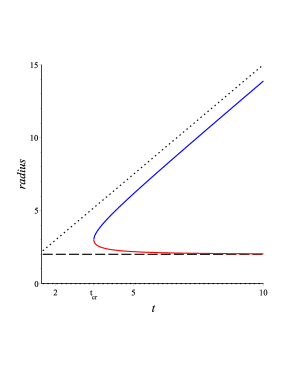
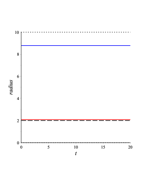
A notable exception arises when the asymptotic spacetime is the de Sitter expanding universe with with the Hubble-de Sitter constant . Then the McVittie metric closes to the Schwarzschild-de Sitter one having the same component (17) with . In this case one obtains a static black hole with static cosmological and black hole horizons as in the right panel of Fig. 1.
However, the principal attribute of the McVittie metric tensor defined by Eqs. (17) and (18) is to be an exact solution of the Einstein equations (9) [9] having the diagonal components
| (23) | |||||
| (24) |
while the component satisfies the condition (12). Thus the presence of this dynamical particle modifies only the fluid pressure, which becomes singular on the entire sphere of radius , but without affecting the density. It is important to observe that this singularity remains outside the physical space domain limited by the black hole horizon of radius . These properties suggest that the McVittie dynamical particles cannot be seen as genuine Schwarzschild-type ones that ought to be produced by a central point singularity in a space-time with flat space sections.
Recently we found a new type of dynamical particles satisfying such exigences. These are defined in new space-times with flat space sections, , having physical frames with line elements of the form
| (25) | |||||
where
| (26) |
In this metric, is the dynamical mass depending on the invariant mass defined as the mass at the initial time when . This metric is an exact solution of Eqs. (9) as in the co-moving physical frames of the space-times the Einstein tensors have isotropic components,
| (27) | |||||
| (28) |
where and are the components of Einstein’s tensor of the asymptotic manifold as given by Eqs. (15) and (16). These solutions describe dynamical particles whose presence gives rise to the additional terms,
| (29) |
which modifies the fluid density as , introducing a central singularity in while the fluid pressure remains unchanged, . These properties encourage us to consider these solutions as Schwarzschild-type dynamical particles or point dynamical particles.
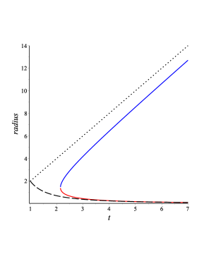
These solutions get physical meaning only inside the physical space domain delimited by the black hole and cosmological horizons whose radii have to be derived by solving the equation for expanding geometries and for collapsing ones [10]. As in the previous case, there is a critical instant such that for we have two positive solutions giving the horizon radii . For understanding their role we considered the expansions [10]
| (30) | |||||
| (31) |
in a time domain where drawing the conclusion that when the time is increasing in expanding universes the cosmological horizon tends to the asymptotic one while the black hole horizon is shrinking to the sphere of radius collapsing then to zero (as in Fig. 2). Note that this property holds even in the case when the asymptotic space-time is the de Sitter expanding universe shown in the right panel of Fig. 2.
| McVittie dyn. particles | Schwarzschild-type dyn. particles | |
| asympt. space-time | any FLRW [9] | spatially flat FLRW |
| static limit | distorted as in Eq. (19) | natural as in Eq. (3) with |
| space sections | curved | flat |
| particle mass | static, | dynamical, |
| black hole horizon | (as in Fig. 1) | (as in Fig. 2) |
| cosm. horizon | ||
| fluid density | unchanged | singular in origin |
| fluid pressure | singular at | unchanged |
Comparing the McVittie and Schwarzschild-type dynamical particles as in Tab. 1 we may conclude that these are systems with different dynamics despite of some general common features as, for example, the existence of the cosmological and black hole horizons. Recently the McVittie dynamical particles have been generalized to manifolds allowing asymptotic FLRW space-times with curved space sections [9]. Therefore we may ask how the Schwarzschild-type ones can be generalized in a non-trivial manner as new solutions of Einstein’s equations with perfect fluid with singular densities but without abandon the spatially flat asymptotic FLRW space-times.
4 New solutions of Einstein’s equations with perfect fluid
In what follows we try to find new solutions of Einstein’s equations in space-times with perfect fluid assuming that these must have: line elements (8) with flat space sections (i. e. ), the asymptotic form (5) and static limit as in Eq. (3).
As in Ref. [10] we consider a class of metrics of the form (25) but with more general functions
| (32) |
depending on the dynamical masses, , which are arbitrary functions of time representing the principal dynamical parameters. The functions and results from Eqs. (9) as
| (33) |
where is an integration constant playing the role of free parameter. We obtain thus the definitive form of the -function,
| (34) |
defining the line elements (25) of the new apace-times we denote from now by referring them as -models. The Einstein tensors of these models have in their proper physical frames the isotropic form
| (35) | |||||
| (36) |
satisfying the condition (12). Thus we may say that the -models defined here are exact solutions of Einstein’s equations with perfect fluid of density and pressure .
For any such model the form of the function (34) guarantees an asymptotic FLRW space-time whose Hubble function satisfies
| (37) |
The Hubble function must be a monotonously time dependent function without zeros in the physical time domain since these might produce singularities of the function giving the radius of the asymptotic horizon. We may prevent these zeros to appear in two cases, either for expanding geometries when we must take
| (38) |
or for collapsing ones for which we have to chose
| (39) |
In what follows we restrict ourselves to the expanding space-times which are of interest in cosmology. Therefore, we have to consider mass functions decreasing monotonously in time and positive parameters .
Integrating then Eq. (37) with the initial condition we obtain the scale factor
| (40) |
of the asymptotic FLRW space-time where such that we preserve the initial condition applied previously to the function (26).
On the other hand, we observe that we may reconstruct these space-times starting with the parameters and recovering the mass function as
| (41) |
and bringing the -function in the form
| (42) |
Under such circumstances the -models may be seen as perturbations of the perfect fluid of their asymptotic space-times. Writing the Einstein tensors in co-moving physical frames as
| (43) | |||||
| (44) |
we understand that these dynamical particles modify only the fluid density preserving its pressure. These perturbations are given by the term
| (45) |
which is singular in and satisfies the expected asymptotic condition .
When we use the parameters , and we denote the space-times by bearing in mind that this is isomorphic with through Eqs. (40) and (41) which relate their parameters. For we recover our point dynamical particles [10],
| (46) |
with -functions of the form (26). However, when we construct the space-times starting with the asymptotic scale factor we must prevent the possible poles in Eq. (41) imposing the restriction where must satisfy
| (47) |
because the function is positively defined.
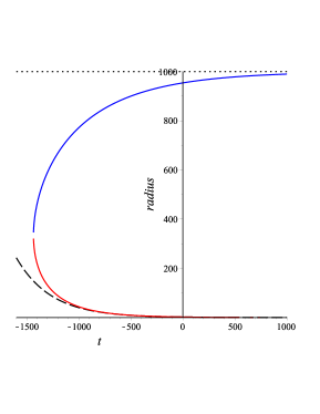
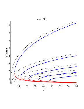
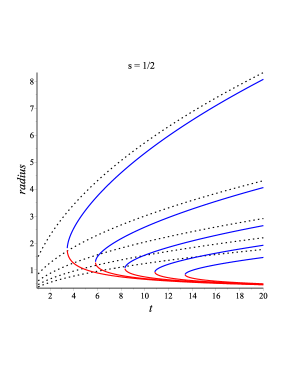
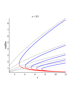
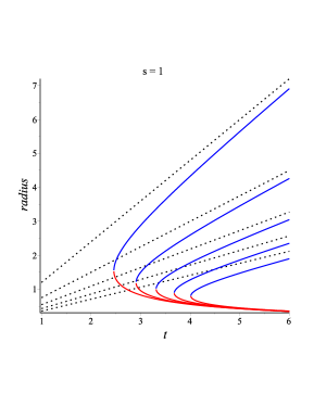
Regardless the parameters we use, the -models describe dynamical particles which behave as black holes inside their physical domains bordered by the spheres of black hole and cosmological horizons. The radii of these horizons have to be derived by solving the equation for expanding universes or for collapsing ones. In both these cases we have to solve cubic equations according to the method presented in the Appendix. The real and positive solutions represent the radii of the black hole and respectively cosmological horizons which arise at the critical time when evolving then in time as C-curves (as in Figs. 3 and 5). In general, for these functions are complicated and less intuitive. Moreover, these cannot be expanded as in Eqs. (30) and (31) because of the parameter which can take arbitrary values. Therefore, for understanding the principal features of the -models we must resort to numerical and graphical analyses.
5 Simple examples
Let us focus now on the simplest examples that could point out the role of the parameter of our new models proposed here without exceeding the performance of usual PC-s in numerical calculations. We restrict ourselves to the -models of expanding space-times which comply with the conditions (38).
Example A We consider first the models of dynamical particles we denote by defined in space-times with
| (48) |
assuming that . In the trivial case of , the mass is static, , and the metric becomes a Schwarzschild-de Sitter one with the line elements in physical frames of the form (7) but with and the Hubble de Sitter constant . The genuine dynamical -models have to be obtained for when the asymptotic behaviour is of FLRW type. The scale factors of the asymptotic space-times derived from Eq. (40) give the radii of the asymptotic horizons (6) as
| (49) |
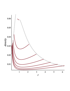
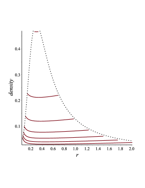
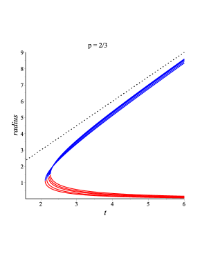
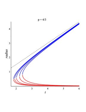
Deriving then the horizon radii (A.9) we may plot in Fig. 3 the evolution of the horizon radii of the -models for various values of parameters and , taking and . These plots show the role of the parameter which determines different asymptotic behaviours of models having the same mass function. Moreover, this parameter is responsible for the profile of the fluid density which carries the singularity in that remains outside the physical domain. Nevertheless, the density in the physical domain feels its effect increasing near the black hole horizon as in Fig. 4. However, for larger values of the density tends to homogeneity (as in the right panel of Fig. 4) which means that this parameter is able to suppress the effect of the singularity when this is increasing enough.
Example B The -models can be constructed using te parameters , and for writing down the metric tensors of the space-times . In this manner we may study families of models having the same asymptotic behaviour determined by the function . Here we consider the simple case of models denoted by having the scale functions
| (50) |
which satisfy our initial condition . In these models the mass functions may be derived as in Eq. (41) but respecting the restriction where
| (51) |
as it results from Eq. (47). This condition guarantees that the mass functions of these models
| (52) |
do not have singularities but restricts severely the values of the parameter . For this reason the models of families with the same asymptotic horizon are very close to each other having horizons whose radii form very similar C-curves as in Fig. 5. Note that we can set only when and the models with any become the dynamical particles of Ref. [10].
In other respects, we observe that the parameter gives some flexibility to our approach such that we may find non-trivial equivalences between different types of models as in the case of the models which are equivalent for any if we set the same values of the constants and .
6 Concluding remarks
We proposed here a new family of space-times depending on a free parameter showing that these represent dynamical particles produced by central singularities of the fluid density but without affecting the pressure of the perfect fluid of the asymptotic FLRW space-times. Each such dynamical particle becomes a black hole at a critical instant when a pair of black hole and cosmological horizons appear on the same sphere. For these horizons evolve creating the physical space between their spheres where a remote observer may perform measurements.
All these models depend on the free parameter resulted as an integration constant when we integrated the Einstein equations. The mass function and this parameter are enough for defining the model determining the time evolution of the entire manifold including the evolution of the cosmological and black hole horizons as well as the scale factor of the asymptotic FLRW space-time. An advantage of our -models is that these can be constructed using an alternative set of parameters formed by the scale factor of the asymptotic FLRW space-time, initial mass and . Regardless the parameters we use remains the typical parameter of our new models. When this parameter vanishes we recover the dynamical particles of Ref. [10] which appear now as a particular cases of the present approach.
As in Ref. [10] we argued that the models with represent a new type of dynamical particles we may conclude that the -models with we proposed and studied here are new dynamical particles that could populate new interesting models of dynamical universes.
Appendix A Solving cubic equations
For solving the cubic equation
| (A.1) |
we substitute first obtaining the modified depressed equation with the coefficients
| (A.2) |
that can be solved using the following form of Cardano’s formulae
| (A.3) | |||||
| (A.4) | |||||
| (A.5) |
where . The cubic equations allow real solutions only when their discriminants are positive, .
The horizons of the McVittie dynamical particles result directly from the depressed equation
| (A.6) |
which has real solutions for where solves the equation obeying . The black hole and cosmological horizons are given by and .
For our -models the cubic equations can be put in the canonical form (A.1) with the coefficients
| (A.7) |
where we denote
| (A.8) |
taking into account that the function is defined by Eq. (34). Finally the solutions we are looking for can be identified as
| (A.9) |
while is the nonphysical solution. Obviously, for we recover the results of Ref. [10].
References
- [1] V. P. Frolov and A. Zelnikov, Introduction to Black Hole Physics (Oxford Univ. Press. Inc., New York 2011).
- [2] C. Gao, X. Chen, Y.-G. Shen, and V. Faraoni, Phys. Rev. D 84, 104047 (2011).
- [3] G. C. McVittie, MNRAS 93 (1933) 325.
- [4] P. Painleve, C. R. Acad. Sci. (Paris) 173 (1921) 677.
- [5] A. Gullstrand, Arkiv. Mat. Astron. Fys. 16 (1922) 1.
- [6] B. C. Nolan, Phys. Rev. D 58 (1998) 064006.
- [7] M. Carrera and D. Giulini, Phys. Rev. D 81 (2010) 043521.
- [8] M. Carrera and D. Giulini, Rev. Modern Phys. 82 (2010) 169.
- [9] R. Nandra, A. N. Lasenby and M. P. Hobson, MNRAS 422 (2012) 2931.
- [10] I. I. Cotăescu, Eur. Phys. J. C 82 (2022) 86.