The probabilistic world II:
Quantum mechanics
from
classical statistics

Abstract

This work discusses simple examples how quantum systems are obtained as subsystems of classical statistical systems. For a single qubit with arbitrary Hamiltonian and for the quantum particle in a harmonic potential we provide explicitly all steps how these quantum systems follow from an overall ”classical” probability distribution for events at all times. This overall probability distribution is the analogue of Feynman’s functional integral for quantum mechanics or for the functional integral defining a quantum field theory. In our case the action and associated weight factor are real, however, defining a classical probabilistic system. Nevertheless, a unitary time-evolution of wave functions can be realized for suitable systems, in particular probabilistic automata. Based on these insights we discuss novel aspects for correlated computing not requiring the extreme isolation of quantum computers. A simple neuromorphic computer based on neurons in an active or quiet state within a probabilistic environment can learn the unitary transformations of an entangled two-qubit system. Our explicit constructions constitute a proof that no-go theorems for the embedding of quantum mechanics in classical statistics are circumvented. We show in detail how subsystems of classical statistical systems can explain various “quantum mysteries”. Conceptually our approach is a straightforward derivation starting from an overall probability distribution without invoking non-locality, acausality, contextuality, many worlds or other additional concepts. All quantum laws follow directly from the standard properties of classical probabilities.

1   The classical and the
quantum world

Why is the world described by quantum mechanics? The answer to this basic question involves three central ingredients Wetterich :

1. The physical description of the universe and its laws is based on probabilities. One may imagine one “overall probability distribution” for all possible events that could happen at different times and locations in our universe. Given the state of the universe at a given time, the probability for most particular events in our rich and complex evolving universe is neither very close to one nor to zero. Then a physical description is not predictive. It will not tell us if on planet earth a certain bee will visit a certain flower around noon on a certain sunny summer day in a garden in Heidelberg. Nevertheless, the classical statistical laws of probabilities can develop strong predictive power for certain questions. This concerns correlations of events, for example sequences of events. If a raindrop has been found at different moments of a time sequence at positions which allow to construct its trajectory and velocity up to a certain time $t$, the conditional probability to find it at the next time step $t+\Delta t$ at a given position may be very close to one or zero. In this case a physicist will predict the position of the drop at $t+\Delta t$ and a physical law for the falling raindrop may be established. The only assumption that we will use is the description of the universe by an overall probability distribution and the standard classical laws for probabilities Kolmogorov (1956). Quantum mechanics and its “axioms” follow once the concept of evolution is introduced and the evolution is unitary. Probabilistic realism Wetterich does not view probabilities as an epistemic description for the lack of knowledge of an observer about some ontological deterministic reality. The overall probability distribution is rather the basic conceptual setting for the description of the universe, similar to the functional integral for quantum field theory.

2. The second ingredient is a time structure of the probabilistic system Wetterich (2012a). We assume that a set of “basis events” can be ordered in some discrete or continuous variable that we call time. The overall probability distribution assigns probabilities to these basis events. We further assume ”locality in time” in the sense that the probability distribution can be written as a product of time-local factors which each involve basis events only at two neighboring times. A simple example is the two-dimensional Ising model Lenz (1920); Ising (1925); Binder (2001) with next-neighbor interactions. The basis events are the configurations of Ising spins on the sites of a two-dimensional lattice. Ising spins take values $\pm 1$ and can be associated with yes/no-decisions or bits in information theory Shannon (1948), or occupation numbers of fermions Wetterich (2017). We may define sequences of hypersurfaces which each divide the two-dimensional lattice into the present (on the hypersurface), the past and future. The choice of the time-hypersurfaces is not unique. We take one such that the interactions between the Ising spins only involve spins on two neighboring hypersurfaces. This implements the time-locality structure. The time-locality structure is not a very particular choice but rather common to many classical statistical systems. One can define a time-local probabilistic information by a suitable sum over events in the past and future. Time-locality permits the notion of evolution according to the simple question: Given the time-local probabilistic information at a certain time $t$, what will be the time-local probabilistic information at the next time step $t+\Delta t$? Most parts of the quantum formalism, namely wave functions or the density matrix encoding the time-local probabilistic information, operators for observables and the evolution operator emerge from the answer to this question. The non-commutative structures between operators characteristic for quantum mechanics are well known for classical statistical systems once they are investigated by the transfer matrix formalism Baxter (1982); Suzuki (1985); Fuchs (1990).

3. Within the large family of classical statistical systems with time locality the specific property which singles out quantum systems is the unitary evolution. For many classical statistical systems much of the initial time-local information is lost as time progresses. For the example of the Ising model we may specify the initial time-local probabilistic information at a given time $t_{0}$, typically on a boundary. As time increases (towards the bulk), the time-local probabilistic information will approach an equilibrium distribution. The rate how fast the more detailed initial information is lost is given by the correlation length. In contrast, for classical statistical systems describing quantum systems the initial information is never lost. Simple examples for “classical” probabilistic systems of this type are probabilistic cellular automata. For cellular automata Ulam (1950); von Neumann (1951); Zuse (1969); Hedlund (1969); Gardner (1970); Richardson (1972); Amoroso and Patt (1972); Hardy et al. (1976); Lindenmayer and Rozenberg (1976); Toom (1978); R. L. Dobrushin (1978); Wolfram (1983); Vichniac (1984); Preston and Duff (1984); Creutz (1986); Toffoli and Margolus (1990); ’t Hooft (2010a, b, 2014); Elze (2014a); LOUIS and Nardi (2018) the updating of the bit-configuration in a local cell is influenced only by a few neighboring cells. Probabilistic cellular automata are defined by a probability distribution over initial configurations. For probabilistic automata a deterministic updating rule guarantees that the initial information is not lost. The preservation of this time-local probabilistic information is the basis for the unitary evolution in quantum mechanics. The deterministic updating maps the probability for a given configuration in the next time step to the probability for the configuration which obtains by the updating. For any probability distribution over initial configurations this defines the overall probability distribution for events at all times. All probabilistic automata are actually quantum systems. Very often it is possible to introduce a complex structure, such that quantum mechanics appears in the familiar form with a complex wave function or density matrix.

If physicists want to describe our highly complex universe, with a rich dynamical evolution of structures seen everywhere, they better employ an overall probabilistic distribution with a time-local structure and unitary evolution Wetterich (1989). Without a unitary evolution most initial probabilistic information would be lost as time progresses, and physicists could only describe some equilibrium state which has not much to do with our universe. The need for a unitary evolution is the need for quantum mechanics, answering the question why we describe the world by quantum mechanics. It is actually sufficient that a large enough subsystem follows a unitary evolution. The remaining part of the time-local probabilistic information can then be seen as an environment for the subsystem which may approach some type of equilibrium. The complex evolution of our world is then described by the subsystem.

In the language of modern quantum field theory we may give a short answer to the question: what is quantum mechanics? The basic description of the world is based on a euclidean functional integral which involves the overall probability distribution for fields or configurations of infinitely many bits. Quantum physics is the projection to the part of the local-time subsystem which follows a unitary evolution. This projection is a quantum field theory in the operator formalism. Quantum mechanics for a few particles or a few qubits follows for appropriate subsystems of the local-time subsystem or quantum field theory.

From this general conceptual setting which is explained in detail in the first part of this work Wetterich , there remains still a long road to go before one understands the properties of a quantum particle in a potential. The reason is that a particle is not a simple object. The historic view has been that particles are simple basic objects, while complexity can be understood, at least in principle, from the interactions of particles. Modern quantum field theory has inverted this view. The quantum field theory for fundamental particles describes infinitely many interacting degrees of freedom. One first needs to find a vacuum state which is a highly complex object – a prime example being the theory of quantum chromodynamics for the strong interactions Wilson (1974); Gattringer and Lang (2010). Particles are seen as excitations of this vacuum. Even a single particle involves infinitely many degrees of freedom. The particle properties are no longer assumed as fundamental. They rather depend on properties of the vacuum. A good example is the mass of the electron which is due to the vacuum expectation value of the Higgs scalar. Actually, in very early cosmology (before the electroweak phase transition) this expectation value vanishes, and so does the electron mass. Quite generally, in cosmology the vacuum corresponds to the dynamical cosmological background solution and therefore depends itself on time.

We should therefore not be surprised if no simple classical statistical system is found for a quantum particle in a potential, or for a few interacting qubits. The classical statistical systems describing fully these simple quantum systems typically involve infinitely many degrees of freedom, similar to the particle in quantum field theory. Nevertheless, reduced quantum features can often be found for classical probability distributions involving only a few degrees of freedom. An example are the realization of discrete subsets of unitary transformations for a few qubits by generalized Ising models of a few classical bits or Ising spins.

The first part of this work Wetterich has developed the general probabilistic view of the world and the concepts of evolution and time. This leads to the quantum formalism for classical statistics Wetterich (2018a). The local factors describing the overall probability distribution for systems with a time-local structure are closely related to the step evolution operator, which is a normalized version of the transfer matrix. The overall probability distribution can be seen as a generalized local chain consisting of a product of local factors. The particular case of unique jump chains realizes a unitary evolution. This case corresponds to probabilistic automata.

In this first part we have developed probabilistic automata which are equivalent to discretized quantum field theories for fermions in one time and one space dimension. For the particular case of free massless fermions the continuum limit of the discrete formulation can be taken and corresponds indeed to the standard quantum field theory of massless free Dirac, Weyl or Majorana fermions in two dimensions. We have established a time- and space-translation invariant vacuum state which respects particle-antiparticle symmetry. All excitations of this vacuum have positive energy, in close analogy to the half-filled Dirac sea in particle physics.

Our discrete analysis of the probabilistic automaton for free massless fermions reveals that already the vacuum state corresponds to a highly non-trivial overall probability distribution. Single particle excitations can be constructed by applying fermionic creation and annihilation operators on this vacuum state. We emphasize that in our approach the basic simple object is directly the quantum field theory, while one-particle quantum mechanics is realized for particular subsystems in a complex setting. This subsystem involves infinitely many degrees of freedom of the overall system. Even though the model is very simple, it is striking how all the concepts of quantum field theory and quantum mechanics emerge in a very natural way from the overall probability distribution. All laws and axioms follow from the standard classical statistical properties of probabilities, without any further assumptions.

In the first part of this work we also have constructed rather simple probabilistic cellular automata which are equivalent to two-dimensional quantum field theories for fermions with interactions. They correspond to generalized Thirring or Gross-Neveu models Thirring (1958); Klaiber (1968); Gross and Neveu (1974); Wetzel (1984); Abdalla et al. (1991); Faber and Ivanov (2001) in a particular discretization. In principle, the path to one-particle quantum mechanics is straightforward to follow. One has to establish the vacuum state for these models and to investigate the properties of the one-particle excitations. In practice, this task is rather complex, however. In the presence of interactions the construction of a particle-antiparticle symmetric vacuum state for which all excitations have positive energy is a rather complicated issue. This influences the form of the possible continuum limit. One expects that important renormalization effects from quantum fluctuations distinguish the true continuum limit from a “naive continuum limit”.

In the present part of this work we approach the construction of one-particle quantum mechanics from the opposite end, starting with only a few classical bits. We keep in mind the basic observation that a quantum particle is a subsystem of a much more complex system, i.e. the quantum field theory. The same holds for the quantum mechanics of a certain number of qubits. Qubits can be seen as a focus on restricted sets of states of a quantum particle. Qubits are in turn subsystems of the quantum mechanics for particles. In principle, we expect that even a single qubit involves infinitely many degrees of freedom of the overall system. In this part of our work we approach the limit of infinitely many degrees of freedom by establishing fundamental concepts leading to quantum mechanics for only a small number of classical bits or Ising spins. We will see how continuous quantum mechanics can emerge in the limit of infinitely many classical bits.

In more detail, we will start from classical probability distributions for only a few discrete degrees of freedom or Ising spins on a given time layer. They can already describe the quantum mechanics of a single qubit for which only a restricted set of unitary transformations is allowed. We will extend this to the full quantum mechanics of a single qubit. This involves indeed infinitely many “classical Ising spins”. We discuss entanglement for classical statistical systems describing two qubits and continue this approach in the direction of several qubits.

This “bottom-up” approach for a few qubits has two important advantages. First, the classical statistical systems are very simple. This allows us to follow very explicitly how the characteristic quantum properties as non-commuting operators or entanglement arise for suitable subsystems of the classical statistical generalized Ising models. The so-called “quantum paradoxes” find explicit solutions in our classical statistical setting, demonstrating how no go theorems for the embedding of quantum mechanics in classical statistics are circumvented.

The second advantage is the direct contact with quantum computing or neuromorphic computing. This highlights the crucial importance of correlations for these types of computing, and points towards more general forms of “correlated computing”. We will show that for two qubits classical statistical systems can realize arbitrary unitary transformations. We demonstrate this by a “model neuromorphic computer” based on spiking neurons. It learns how to perform the complete set of the well known basic quantum gates. Suitable sequences of these gates result in arbitrary unitary transformations for the two-qubit quantum subsystem. This demonstrates that the performance of certain quantum tasks does not need the high degree of isolation of a quantum system often assumed to be necessary. These tasks could be performed under “human conditions”, for example by our brain. On the other hand, an extension to full quantum operations for many qubits requires a highly complex control of correlations. This underlines the great prospects of “real” quantum computers for which the nature of atoms as quantum objects guarantees the correlations necessary for quantum computing. One may envisage the possibility that intermediate forms of correlated computing, which do not perform arbitrary unitary transformations for entangled qubits, could still be used by macroscopic systems without extreme isolation, as the human brain.

In summary, quantum mechanics and “classical” probabilistic systems are in a much closer relation than commonly realized. In short, quantum systems are particular types of subsystems of general “classical” probabilistic systems. The general properties of subsystems and their relation to quantum mechanics are the central topic of this work. We will see how all the “mysterious” properties of quantum systems arise in a natural way from the generic properties of subsystems. The correlations of subsystems with their environment play an important role in this respect, leading to many features familiar from quantum mechanics. These features are not realized for the often considered uncorrelated subsystems. The presence of various quantum features in classical statistical systems has been proposed in different settings in refs. Hardy (2001); Kirkpatrick (2003); Barrett (2007); Fuchs and Schack (2013); Camsari et al. (2017); Budiyono and Rohrlich (2017); Camsari et al. (2019); Yavuz and Yadav (2023a, b); Chowdhury et al. (2023). We advocate here the viewpoint that all quantum features actually arise from suitable classical probabilistic systems Wetterich (2001, 2004, 2009).

In sect. 2 we discuss a first simple discrete quantum system for a single qubit. It is based on a local chain for three Ising spins at every time-layer $t$. Already this simple system shows many features of quantum mechanics, as the whole formalism and particle-wave duality. We recall in this section several key concepts of this work, as the classical wave function and density matrix, the step evolution operator, or the status of observables and associated operators. These concepts are described in detail in ref. Wetterich . We proceed in sect. 3 to entangled systems, both entangled quantum systems and entangled classical probabilistic systems. Entanglement is not a property particular to quantum mechanics. We construct explicitly entangled classical probabilistic systems which lead to entangled two-qubit quantum subsystems.

In sect. 4 we take the limit of continuous variables for the description of a classical probabilistic system. It obtains for an infinite number of Ising spins or yes/no decisions. All properties follow from the case of discrete variables by taking a suitable limit. There is no practical difference between continuous variables and a very large number of discrete variables. In this respect the continuum description is rather a matter of convenience. Nevertheless, the continuum limit often shows universal features which lead to important simplifications. The equivalence of continuous variables with an infinite number of discrete variables is at the basis of an important property of the one-qubit quantum system. The quantum system has an infinity of observables with only two possible measurement values. These are given by the quantum spin in arbitrary directions. The yes/no decisions associated to continuous classical variables can be mapped to the two-level observables in the quantum subsystem.

In sect. 5 we address continuous quantum mechanics. We first discuss the dynamics of a single qubit with an arbitrary time-dependent Hamiltonian. It is based on a classical statistical system with a probability distribution depending on continuous variables. A continuous set of yes/no questions is mapped to a continuous set of quantum observables corresponding to the quantum spin in different directions. The possible measurement values are discrete, as given by the eigenvalues of the associated quantum operators. The classical overall probability distribution realizes both sides of quantum mechanics: the continuous wave function and the discrete observables. As it should be, the quantum operators for spins in different directions do not commute. Their expectation values obey the uncertainty relations of quantum mechanics. This is related to the presence of ”quantum constraints” for the subsystem which enforce correlations between the spin in different directions. In this section we also construct a simple probabilistic automaton which describes a quantum particle in a harmonic potential. It is based on the classical statistical Liouville equation in phase space for a particle with two colors. Suitable initial conditions lead to color oscillations with periods predicted by the equidistant spectrum of the Hamiltonian of the quantum subsystem. This underlines the usefulness of the quantum description for the understanding of the dynamics of classical statistical systems.

In sect. 6 we turn to a possible use of our setting for computing. Classical and quantum computing are treated in the same general setting of probabilistic computing as different limiting cases. Many intermediate cases between the two limits could lead to new powerful computational structures. In particular, we address artificial neural networks and neuromorphic computing within our general setting and ask if computers constructed according to these principles, or even biological systems as the human brain, could perform quantum operations. We provide examples where this is the case for simple systems of spiking neurons. Since these systems are “classical”, this demonstrates in a very direct way that there are no conceptual boundaries between classical probabilistic systems and quantum systems.

In sect. 7 we turn to the important topic of conditional probabilities and their relations to sequences of measurements. Most of the questions that humans ask about Nature invoke conditional probabilities, of the type “if an experimental setting is prepared, what will be the probability for a certain outcome under this condition”. Conditional probabilities are closely related to different types of measurements. In particular, one has to think about the notion of “ideal measurements” for subsystems. The “reduction of the wave function” turns out to be a convenient mathematical tool for the description of conditional probabilities, rather than a physical process. The concepts of conditional probabilities and ideal measurements for subsystems play an important role for our discussion of the “paradoxes” of quantum mechanics in sect. 8. There we address Bell’s inequalities, the Kochen-Specker no-go theorem and the Einstein-Podolski-Rosen paradox. They all find a natural explanation in our “classical” probabilistic setting.

We conclude in sect. 9 by a short overview of the embedding of quantum mechanics in classical statistical systems. In particular, we address a list of often asked questions about the origin of various aspects of quantum mechanics. We provide short answers how these quantum features emerge from classical statistics if one focuses on appropriate subsystems.

2   Qubit automaton

Quantum mechanics is realized for local subsystems with unitary evolution. For a given quantum state, as characterized by the quantum density matrix $\rho(t)$, or wave function $\psi(t)$ for the special case of a pure quantum state, only the local probabilistic information at $t$ is used. We will express $\rho(t)$ in terms of the time-local probability distribution $\{p_{\tau}(t)\}$ for three classical Ising spins. The quantum subsystem typically does not use all the local information contained in $\{p_{\tau}(t)\}$. A few particular expectation values or classical correlations of the Ising spins $s_{\gamma}(t)$ specify the subsystem. The evolution law of the subsystem is inherited from the evolution law of the underlying local chain. It describes a linear unitary evolution of the density matrix, such that no information contained in the quantum subsystem is lost. Our quantum subsystem admits a complex structure. In the complex formulation the density matrix is Hermitian and normalized,

$$\rho^{\dagger}(t)=\rho(t), tr\rho(t)=1.$$ (2.0.1)

An important property is the positivity of the density matrix, i.e. the property that all its eigenvalues are positive or zero.

In the present section we concentrate on quantum mechanics for a single qubit. A simple local chain with three classical Ising spins realizes already many characteristic features of quantum mechanics, as non-commuting operators for observables, the quantum rule for the computation of expectation values, discrete measurement values corresponding to the spectrum of operators, the uncertainty principle, unitary evolution and complex structure.

2.1   Discrete qubit chain

Let us consider a simple automaton for three classical bits or Ising spins $s_{k}=\pm 1$. With probabilistic initial conditions the overall probability distribution is given by a local chain with three Ising spins $s_{k}(t)$ or $s_{k}(m)$, $k=1,2,3$, at every discrete position $m$. The discrete qubit chain is a unique jump chain for which each orthogonal step evolution operator maps $s_{k}=s_{k}(m)$ to $s_{k}^{\prime}=s_{k}(m+1)$. The order of these operators in the chain is left arbitrary. We employ six basis operators and products thereof,

$$\begin{split}T_{12}:\ s_{1}^{\prime}=s_{2},\ \quad s_{2}^{\prime}=-s_{1},\\ T_{23}:\ s_{2}^{\prime}=s_{3},\ \quad s_{3}^{\prime}=-s_{2},\\ T_{31}:\ s_{3}^{\prime}=s_{1},\ \quad s_{1}^{\prime}=-s_{3},\\ T_{1}:\ s_{2}^{\prime}=-s_{2},\quad s_{3}^{\prime}=-s_{3},\\ T_{2}:\ s_{1}^{\prime}=-s_{1},\quad s_{3}^{\prime}=-s_{3},\\ T_{3}:\ s_{1}^{\prime}=-s_{1},\quad s_{2}^{\prime}=-s_{2}.\end{split}$$ (2.1.1)

The Ising spins not listed explicitly remain invariant. The first three transformations correspond to $\pi/2$ rotations of the spin $s_{k}$ in different “directions”, where $k=1,2,3$ may be associated to three “coordinate directions”, say $x,y,z$. The three last transformations are combined reflections of two spins. We also admit all products of the six transformations (2.1.1). The transformations form a discrete group.

The unique jump operators $\hat{S}(m)$ may differ for different $m$. The different transformations do not commute, such that for $\hat{S}(m)$ depending on $m$ the order of the matrices according to $m$ matters for the overall probability distribution and the expectation values of local observables. A given sequence of $\hat{S}(m)$ could correspond to a deterministic classical computer with three bits $s_{k}$. This is realized if the initial state is a fixed spin configuration. In contrast, we will consider here probabilistic initial conditions by specifying at some initial $m$, say $m=0$, the probabilities $p_{\tau}$ for each configuration $\tau$. This defines a probabilistic automaton. We will restrict the initial probability distribution to obey a certain “quantum constraint”. The layers $m$ in the local chain may be a time sequence, but they could also label any other sequence, for example an order in space, or layers in a neural network. We will see that the discrete qubit chain can also be viewed as an embryonic quantum computer.

For three bits there are eight classical states, $\tau=1,...,8$, that we may label by eight different spin configurations, e.g. in the order $(---),$ $(--+),$ $(-+-),$ $(-++),$ $(+--),$ $(+-+),$ $(++-),$ $(+++)$ for $\tau$ from 1 to 8. The eight time-local probabilities $p_{\tau}(m)$ are the probabilities for these configurations on the layer $m$. The expectation values of the three spins follow the basic probabilistic rule

$$\rho_{k}(m)=<s_{k}(m)>=\sum_{\tau}p_{\tau}(m)(S_{k})_{\tau},$$ (2.1.2)

with $(S_{k})_{\tau}$ the value of the spin observable in the state $\tau$, e.g.

$$\begin{split}(S_{1})_{\tau}&=(-1,-1,-1,-1,\ 1,\ 1,\ 1,\ 1),\\ (S_{2})_{\tau}&=(-1,-1,\ 1,\ 1,-1,-1,\ 1,\ 1),\\ (S_{3})_{\tau}&=(-1,\ 1,-1,\ 1,-1,\ 1,-1,\ 1).\end{split}$$ (2.1.3)

2.2   Classical wave function and step
evolution operator

A convenient formalism for probabilistic automata is based on the real classical wave function. Its components $q_{\tau}(m)$ obey

$$p_{\tau}(m)=q_{\tau}^{2}(m)\ .$$ (2.2.1)

For arbitrary $q_{\tau}$ the probabilities $p_{\tau}$ are positive, $p_{\tau}\geq 0$. The normalization of the probability distribution is guaranteed if $q_{\tau}$ are the components of a unit vector. Any change of the probability distribution with time results in a simple rotation of this unit vector. The step evolution operator $\hat{S}(m)$ performs this rotation

$$q_{\tau}(m+1)=\hat{S}_{\tau\rho}(m)q_{\rho}(m)\ .$$ (2.2.2)

It is therefore an orthogonal matrix – in our case an $8\times 8$ matrix.

A classical density matrix $\rho^{\prime}(m)$ can be constructed as a bilinear of the classical wave function, with elements

$$\rho^{\prime}_{\tau\rho}(m)=q_{\tau}(m)q_{\rho}(m)\ .$$ (2.2.3)

We can express the expectation values (2.1.2) in terms of the classical density matrix $\rho^{\prime}(m)$, which is a real $8\times 8$ matrix, as

$$\rho_{k}(m)=\langle s_{k}(m)\rangle=tr\left(\hat{S}_{k}\rho^{\prime}(m)\right),$$ (2.2.4)

with diagonal classical spin operators

$$(\hat{S}_{k})_{\tau\rho}=(S_{k})_{\tau}\delta_{\tau\rho}.$$ (2.2.5)

Only the diagonal elements $p_{\tau}(m)=\rho^{\prime}_{\tau\tau}(m)$ contribute in this expression. The classical spin operators commute among themselves, but do not commute with the step evolution operator, except for those spins that remain invariant under a given transformation $T_{a}$. A similar expression in terms of the classical wave function is the analogue of the quantum law

$$\langle s_{k}(m)\rangle=q_{\tau}(m)\big{(}\hat{S}_{k}\big{)}_{\tau\rho}q_{\rho}(m)\ .$$ (2.2.6)

The overall probability distribution for probabilistic automata is rather easily visualized. For each initial configuration $\tau_{0}$ we can construct the trajectory by applying the updating rule of the automaton. This trajectory is the sequence of configurations reached by the updating. Each point on the trajectory has the same probability, given by the initial probability $p_{\tau_{0}}(0)$. Every configuration of spins $\{s_{k}(m)\}$ belongs to a unique trajectory. In this way one assigns overall probabilities to all configurations $\{s_{k}(m)\}$ which can be constructed from the spins at all $m$. The step evolution operators (2.2.2) are constructed in order to realize this overall probability distribution.

For all probabilistic automata the step evolution operators are unique jump matrices. They have in each row and column precisely one element equal to one or minus one, and all other elements zero. For each one of the transformations (2.1.1) we can construct an associated step evolution operator. This is done by following how each one of the eight configurations $\tau$ is mapped by the operation of $T$ to a new configuration. We do not need the explicit form of the step evolution operators $\hat{S}(m)$ for the present purpose and refer to ref. Wetterich for their explicit construction for cellular automata.

The unique jump step operators transform the local probabilities among themselves as a limiting case of a Markov chain without loss of information. This transformation reproduces for the expectation values $\rho_{k}=\langle s_{k}\rangle$ the same transformation as for the spins $s_{k}$, e.g. for $\hat{S}(m)$ corresponding to $T_{12}$ one has $\rho_{1}(m+1)=\rho_{2}(m)$, $\rho_{2}(m+1)=-\rho_{1}(m)$, $\rho_{3}(m+1)=\rho_{3}(m)$. (There should be no confusion between expectation values $\rho_{k}(m)$ and elements of the classical density matrix $\rho_{\tau\rho}^{\prime}(m)$.) We also do not need here the explicit form of the overall probability distribution. It is sufficient to realize that it exists in order to see that we deal with a classical statistical system. For a detailed discussion of the realization of the overall probability distribution as a constrained generalized Ising model we refer to ref. Wetterich .

2.3   Quantum subsystem

It is a key property of many quantum systems that they are subsystems of more extended classical probabilistic systems. The resulting incomplete statistics is the origin of the uncertainty relation and the non-commuting operator structure. We discuss the quantum subsystem for the discrete qubit chain here. We could already interpret the discrete qubit chain as a type of discrete quantum mechanics with real wave functions. This quantum system is somewhat boring since all operators commute and everything looks as a trivial reformulation of simple classical properties. We will show that the restriction to a subsystem can change these properties profoundly, leading to complex discrete quantum mechanics with non-commuting operators for the spin observables. On the one hand, the map to the subsystem discards part of the information contained in the time-local probability distribution $\{p_{\tau}(m)\}$ for the discrete qubit chain. The information retained for the subsystem exceeds, however, the one in a classical probability distribution for two or less classical bits. We can still compute all three expectation values $\rho_{k}(m)$ from the information contained in the subsystem.

Time-local subsystem

The quantum subsystem is based on the three expectation values $\rho_{k}(m)$. For every given $m$ it is a time-local subsystem. It is also a simple form of a subsystem based on correlations. (See ref Wetterich for a general discussion of subsystems based on correlations.) The three values $\rho_{k}(m)$ are the only information used by and available to the subsystem. The evolution of the discrete qubit chain transforms the expectation values among themselves and thus the subsystem is closed under the evolution. The subsystem uses only part of the local probabilistic information in the form of three particular combinations of local probabilities,

$$\begin{split}\rho_{1}=-p_{1}-p_{2}-p_{3}-p_{4}+p_{5}+p_{6}+p_{7}+p_{8}\ ,\\ \rho_{2}=-p_{1}-p_{2}+p_{3}+p_{4}-p_{5}-p_{6}+p_{7}+p_{8}\ ,\\ \rho_{3}=-p_{1}+p_{2}-p_{3}+p_{4}-p_{5}+p_{6}-p_{7}+p_{8}\ .\end{split}$$ (2.3.1)

Quantum density matrix and quantum operators

We collect the probabilistic information for the quantum subsystem in the form of a Hermitian $2\times 2$ matrix Wetterich (2009)

$$\rho=\frac{1}{2}(1+\rho_{k}\tau_{k}), \rho^{\dagger}=\rho, tr\ \rho=1.$$ (2.3.2)

Hermiticity follows for real $\rho_{k}$ from the hermiticity of the Pauli matrices $\tau_{k}$, and $tr\ \rho=1$ follows from $tr\ \tau_{k}=0$. This matrix is the quantum density matrix describing the subsystem, provided that it is a positive matrix, see below in sect. 2.5.

We introduce three Hermitian quantum operators $S_{k}$ for the three “Cartesian directions” of the qubit, given by the Pauli matrices,

$$S_{k}=\tau_{k}, S_{k}^{\dagger}=S_{k}.$$ (2.3.3)

In terms of these quantum operators we can compute for every $m$ the expectation values of the classical spins from the density matrix,

$$\langle s_{k}\rangle=\rho_{k}=tr\ (\rho S_{k}).$$ (2.3.4)

This follows from $tr(\tau_{k}\tau_{l})=2\delta_{kl}$, $tr\ \tau_{k}=0$,

$$\rho_{k}=\frac{1}{2}tr\left\{(1+\rho_{l}\tau_{l})\tau_{k}\right\}=\frac{1}{2}\rho_{l}\delta_{lk}\ tr\ 1.$$ (2.3.5)

We identify the three components of the quantum spin or qubit with the three classical Ising spins $s_{k}$,

$$\langle S_{k}\rangle_{q}=\langle s_{k}\rangle_{cl}.$$ (2.3.6)

Here$\langle s_{k}\rangle_{cl}$ is computed according to the classical rule, while $\langle S_{k}\rangle_{q}$ is computed according to the quantum rule which associates to every observable $A$ an Hermitian operator and computes the expectation value from the density matrix

$$\langle A\rangle=tr(\rho A).$$ (2.3.7)

We emphasize that with the identification (2.3.6) the quantum rule (2.3.7) is no independent new rule or axiom. It follows directly from the classical probabilistic definition of expectation values.

The classical spin operators $\hat{S}_{k}$ in eq. (2.2.5) and the quantum spin operators $S_{k}$ in eq. (2.3.3) are different objects. The classical spin operators $S_{k}$ are real diagonal $8\times 8$ matrices and commute. The quantum spin operators $\hat{S}_{k}$ are Hermitian $2\times 2$ matrices that do not commute,

$$\left[S_{k},S_{l}\right]=2i\varepsilon_{klm}S_{m}.$$ (2.3.8)

For distinction, we use a hat for classical operators and no hat for quantum operators. The map to the subsystem maps commuting ”classical” operators to non-commuting quantum operators Wetterich (2010a).

Particle-wave duality

Already in this very simple form we see the particle-wave duality of quantum mechanics. The possible measurement values of the quantum spin components are $\pm 1$, as given by the possible measurement values of the three classical Ising spins $s_{k}$. The possible measurement values of the quantum spin are the eigenvalues of the spin operators $S_{k}$. The quantum rule states that the possible measurement values of an observable are given by the spectrum of the associated operator. This is not a new rule or axiom, but follows from the association with the classical Ising spins. The discreteness of the possible measurement values is the “particle side” of particle-wave duality.

The “wave-side” is the continuous character of the time-local probabilistic information. The probabilities $p_{\tau}$, and therefore the expectation values $\rho_{k}$ in eq.(2.3.1), are continuous. The density matrix is continuous as well. The density matrix $\rho$ is a “pure state density matrix” if it obeys the condition

$$\rho^{2}=\rho.$$ (2.3.9)

In this case $\rho$ can be composed as a product of the pure state wave function $\psi$ and its complex conjugate $\psi^{*}$ according to

$$\rho_{\alpha\beta}=\psi_{\alpha}\psi_{\beta}^{*}.$$ (2.3.10)

The wave function is a normalized two component vector, $\psi^{\dagger}\psi=1$, which is an element of Hilbert space. The overall phase of $\psi$ plays no role since it does not appear in the density matrix (2.3.10). All the wave-aspects of quantum mechanics are associated to the continuous character of the local probabilistic information.

For the particular case of a pure quantum state the rule (2.3.7) for the expectation value of an observable takes the form familiar from quantum mechanics

$$\langle A\rangle=tr(\rho A)=\rho_{\beta\alpha}A_{\alpha\beta}=\psi_{\alpha}^{*}A_{\alpha\beta}\psi_{\beta}.$$ (2.3.11)

It may be written in the conventional bra-ket notation as

$$\langle A\rangle=\psi^{\dagger}A\psi=\bra{\psi}A\ket{\psi}.$$ (2.3.12)

We see that already for the simple one qubit subsystem the rules of quantum mechanics emerge in a natural way.

2.4   Incomplete statistics

The operators for the quantum spins do not commute. This is no accident or result of some particular choice. It is a direct consequence of the quantum subsystem being characterized by incomplete statistics Wetterich (2001, 2004). Incomplete statistics is defined here in the sense that the statistical information in the subsystem is not sufficient to compute classical correlation functions for all observables.

Quantum subsystem and environment

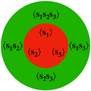
Figure 1: Schematic embedding of the quantum subsystem within the classical statistical system in the space of correlation functions. The inner region (red) comprises the quantum subsystem, and the outer region (green) constitutes the environment. In contrast, a “classical subsystem” would eliminate $s_{1}$, consisting of the correlations $s_{2}$, $s_{3}$ and $s_{2}s_{3}$. The quantum subsystem is clearly not of this type.

The quantum subsystem is characterized by the three expectation values $\langle s_{k}\rangle$. All other classical correlation functions of the Ising spins, as $\langle s_{k}s_{l}\rangle$ or $\langle s_{1}s_{2}s_{3}\rangle$, belong to the “environment”. This is depicted in Fig. 1. The quantum subsystem can be seen as a submanifold in the manifold of all classical correlation functions of Ising spins at a given $m$. In terms of the local probabilities $p_{\tau}$ the quantum subsystem is a three-dimensional submanifold of the seven-dimensional manifold of the independent local probabilities, specified by the relations (2.3.1). The other four independent combinations of $p_{\tau}$ specify the environment, but are not relevant for the quantum subsystem. For a given $(\rho_{1},\rho_{2},\rho_{3})$ all local probability distributions leading to the same $\rho$ describe the same quantum subsystem. The map from the local probability distribution to the quantum subsystem is not invertible. It “forgets” the probabilistic information pertaining to the environment.

Classical correlation functions

The classical two-point and three-point correlation functions belong to the environment, and not to the quantum subsystem. They cannot be computed from the probabilistic information of the quantum subsystem. For example, one has

$$\langle s_{1}s_{2}\rangle=p_{1}+p_{2}-p_{3}-p_{4}-p_{5}-p_{6}+p_{7}+p_{8}.$$ (2.4.1)

This linear combination cannot be expressed in terms of $\rho_{k}$. Classical correlations are “inaccessible” for the quantum subsystem, since their computation needs information about the environment beyond the subsystem. This is “incomplete statistics”. For incomplete statistics the probabilistic information is sufficient for the computation of expectation values of a certain number of observables, but insufficient for the computation of all classical correlation functions for these observables. For more general systems of incomplete statistics some of the correlation functions may belong to the subsystem, but not all of them. We will encounter this case for two qubits in sect. 3.2.

Incomplete statistics and non commuting operators

For an expression of expectation values by eq. (2.3.7) not all operators for observables of the incomplete statistical system can commute. This is the basic origin for the non-commutativity of the quantum spin operators for the discrete qubit chain.

If two quantum operators $A$ and $B$ commute, $[A,B]=0$, also the product $C=AB=BA$ is a valid quantum operator that commutes with $A$ and $B$. The expectation values of $A$, $B$ and $C$ are independent real numbers that have to be part of the probabilistic information in the quantum subsystem. More precisely, $\langle C\rangle$ is restricted by the values of $\langle A\rangle$ and $\langle B\rangle$, but not computable in terms of $\langle A\rangle$ and $\langle B\rangle$ except for the particular limiting cases $\langle A\rangle=\pm 1$, $\langle B\rangle=\pm 1$. If we associate $A$ with $s_{1}$ and $B$ with $s_{2}$ we have one more quantum observable $D$ associated with $s_{3}$. Since $\langle D\rangle$ cannot be expressed in terms of $\langle A\rangle$,$\langle B\rangle$ and $\langle C\rangle$, such a system would need at least the probabilistic information given by four real numbers. This is more than available by a $2\times 2$ Hermitian normalized density matrix. The assumption $[A,B]=0$ leads to a contradiction. One concludes that the operators representing the three classical spins $s_{k}$ in the subsystem cannot commute. This holds for every pair of quantum operators $S_{k}$.

It is interesting to consider for an extended setting the particular case where the quantum correlation $\langle AB\rangle_{q}$ of two commuting quantum observables equals the classical correlation $\langle AB\rangle_{cl}$ for two classical observables $A$ and $B$ whose expectation values are used for the definition of the quantum subsystems, i.e. $\langle A\rangle_{q}=\langle A\rangle_{cl}$, $\langle B\rangle_{q}=\langle B\rangle_{cl}.$ While this is not the general case, we will discuss in sect. 3.4 an interesting “correlation map” where this is realized. In this case one has

$$\langle AB\rangle_{q}=tr(\rho AB)=\langle AB\rangle_{cl}=\sum_{\tau}p_{\tau}A_{\tau}B_{\tau}.$$ (2.4.2)

This identity can hold only for commuting quantum operators. Indeed, for any two commuting operators there exists a basis where both are diagonal,

$$A_{\alpha\beta}=A_{\alpha}\delta_{\alpha\beta}, B_{\alpha\beta}=B_{\alpha}\delta_{\alpha\beta},$$ (2.4.3)

with $A_{\alpha}$ and $B_{\alpha}$ given by possible measurement values of the observables. In this basis one has

$$\langle AB\rangle_{q}=\sum_{\alpha}\rho_{\alpha\alpha}A_{\alpha}B_{\alpha},$$ (2.4.4)

which corresponds precisely to the classical expectation value $AB_{cl}$, provided that the diagonal elements $\rho_{\alpha\alpha}$ can be associated with probabilities of a subsystem of the classical system.

More precisely, for two-level observables $A$ and $B$ with possible measurement values $\pm 1$ the “simultaneous probability” $p_{++}$ for finding $A=+1$ and $B=+1$ is computable as an appropriate combination of diagonal elements $\rho_{\alpha\alpha}$. This also holds for the other simultaneous probabilities $p_{+-}$, $p_{-+}$ and $p_{--}$. The same simultaneous probabilities are computable from the classical probabilities $p_{\tau}$. The relation (2.4.2) requires that all simultaneous probabilities are the same in the quantum subsystem and the classical statistical system. On the other hand, simultaneous probabilities are not available for the quantum system if two associated operators do not commute. (An exception may be states for which $\langle[A,B]\rangle$ vanishes.) The two operators $A$ and $B$ cannot be diagonalized simultaneously. In a basis where $A$ is diagonal, linear combinations of the positive semidefinite diagonal elements $\rho_{\alpha\alpha}$ can be employed to define the probabilities to find $A=1$, or $A=-1$. Similar probabilities can be computed for $B$ in a basis where $B$ is diagonal. There is no way, however, to extract simultaneous probabilities.

We conclude the following properties: If the classical correlation function $\langle AB\rangle_{cl}$ is part of the probabilistic information of the quantum subsystem, the associated quantum operators $A$ and $B$ have to commute. Inversely, if $A$ and $B$ do not commute, the classical correlation function is not available for the quantum subsystem and therefore belongs to the environment. If $A$ and $B$ commute, the classical correlation function can belong to the quantum subsystem but does not need to. It may also be part of the environment. This issue depends on the precise implementation of the quantum subsystem.

2.5   Quantum condition

In order to realize a quantum subsystem the three expectation values $\rho_{k}=\langle s_{k}\rangle_{cl}$ have to obey an inequality

$$\sum_{k}\rho_{k}^{2}\leq 1.$$ (2.5.1)

This “quantum constraint” or “quantum condition” arises from the requirement that the quantum density matrix $\rho$ is a positive matrix. Pure quantum states require the “pure state condition”

$$\rho_{k}\rho_{k}=1,$$ (2.5.2)

while mixed states obey

$$\rho_{k}\rho_{k}<1.$$ (2.5.3)

The quantum subsystem can therefore not be realized for arbitrary time-local probabilities $\{p_{\tau}(m)\}$, but only for a submanifold defined by eq. (2.5.1). We will see that the quantum constraint is preserved by the evolution. It has important consequences for the expectation values in the quantum subsystem.

The quantum constraint arises here as a condition for the realization of a subsystem with closed time evolution. There are some analogues with restricted classical probability distributions which induce certain quantum features Caves and Fuchs (1996); Hardy (1999); Fuchs (2002); Spekkens (2007); Harrigan and Spekkens (2010); Bartlett et al. (2012). Our general idea is that suitable subsystems are selected by the evolution dynamics of the overall probability distribution in a context of infinitely many degrees of freedom, similar to isolated atoms in a quantum field theory. This dynamical selection can impose the quantum constraint. For the purpose of our example we simply postulate the quantum constraint.

Pure state condition

Consider first the pure state condition (2.5.2). For a pure quantum state one needs the condition (2.3.9). We write the definition (2.3.2) of the quantum subsystem as

$$\rho=\frac{1}{2}\rho_{\mu}\tau_{\mu},$$ (2.5.4)

where we employ

$$\tau_{0}=1, \rho_{0}=1,$$ (2.5.5)

and that the sum over $\mu$ extends form zero to three. The condition $\rho^{2}=\rho$ amounts to

$$\frac{1}{4}(\rho_{\mu}\tau_{\mu})(\rho_{\nu}\tau_{\nu})=\frac{1}{8}\rho_{\mu}\rho_{\nu}\{\tau_{\mu}\tau_{\nu}\}=\frac{1}{2}\rho_{\mu}\tau_{\mu}.$$ (2.5.6)

With $\{\tau_{k},\tau_{l}\}=2\delta_{kl}$, $\{\tau_{k},\tau_{0}\}=2\tau_{k}$, $\{\tau_{0},\tau_{0}\}=2$ the condition (2.5.6) becomes

$$\frac{1}{4}(1+\rho_{k}\rho_{k})+\frac{1}{2}\rho_{k}\tau_{k}=\frac{1}{2}+\frac{1}{2}\rho_{k}\tau_{k},$$ (2.5.7)

which indeed requires the condition (2.5.2). Inversely, eq. (2.5.2) implies a pure state density matrix $\rho^{2}=\rho$.

Positive eigenvalues of density matrix

For a pure quantum state the two eigenvalues of $\rho$ are $\lambda_{1}=1$, $\lambda_{2}=0$. In general, the positivity of $\rho$ requires $\lambda_{1}\geq 0$, $\lambda_{2}\geq 0$. From

$$\mathrm{tr}(\rho)=\lambda_{1}+\lambda_{2}=1, \det(\rho)=\lambda_{1}\lambda_{2},$$ (2.5.8)

we conclude that $\rho$ is a positive matrix if $\det(\rho)\geq 0$. Computing from eq. (2.5.4)

$$\det(\rho)=\frac{1}{4}(1-\rho_{k}\rho_{k}),$$ (2.5.9)

the condition $\det(\rho)\geq 0$ indeed coincides with the quantum constraint (2.5.1). The boundary value $\det(\rho)=0$ is realized for the pure state condition (2.5.2), as appropriate since one eigenvalue of $\rho$ vanishes. We conclude that mixed quantum states with positive $\rho$ not obeying $\rho^{2}=\rho$ require the inequality (2.5.3).

Bloch sphere

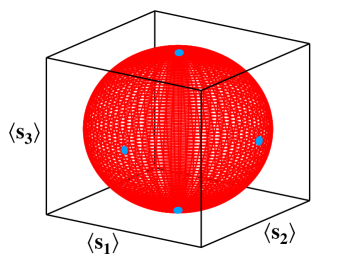
Figure 2: Quantum condition. For a quantum subsystem the expectation values $s_{z}$ must be inside or on the Bloch sphere. Points on the Bloch sphere are pure quantum states. Points outside the Bloch sphere correspond to classical statistical probability distributions that do not realize a quantum subsystem. Corners of the cube have $|s_{k}|=1$ for all $k$ and are not compatible with the quantum subsystem. The Bloch sphere touches the cube at the points indicated at the center of its surfaces.

The quantum condition is visualized in Fig. 2. Pure quantum states are points on the Bloch sphere with $\braket{s_{1}}^{2}+\braket{s_{2}}^{2}+\braket{s_{3}}^{2}=1$. The mixed quantum states correspond to points inside the Bloch sphere.

Uncertainty relation

The most general classical probability distributions for three Ising spins can realize arbitrary values $\braket{s_{k}}$ in the interval $-1\leq\braket{s_{k}}\leq 1$. These correspond to all points inside the cube in Fig. 2. Points inside the cube but outside the Bloch sphere are valid classical probability distributions, but the associated probability distributions do not admit a quantum subsystem. Quantum subsystems can therefore be only realized by a subfamily of classical probability distributions. The non-invertible map from the classical probability distribution $\{p_{\tau}\}$ to the matrix $\rho$ can be defined by eq. (2.5.4) for arbitrary $\{p_{\tau}\}$. Only for a submanifold of $\{p_{\tau}\}$ the matrix $\rho$ describes a valid positive quantum density matrix, however.

As an example we consider the limiting classical distribution for which $p_{\tau}$ differs from zero only for the particular state with $s_{1}=s_{2}=1$, $s_{3}=-1$. This translates to $\braket{s_{1}}=\braket{s_{2}}=1$, $\braket{s_{3}}=-1$ and corresponds to one of the corners of the cube in Fig. (2). With $\rho_{k}\rho_{k}=3$ this classical probability distribution violates the quantum constraint (2.5.1). Indeed, no valid quantum state can realize simultaneously fixed values for the quantum spin in all directions.

More generally, the uncertainty relation of quantum mechanics follows directly from the quantum constraint. Indeed, for a positive Hermitian normalized density matrix $\rho$ the formulation of quantum mechanics can be applied and induces the uncertainty relation. We can see directly from the quantum condition (2.5.1) that a sharp value $\braket{s_{1}}=\pm 1$ requires a vanishing expectation value for the spins in the two other Cartesian directions, $\braket{s_{2}}=\braket{s_{3}}=0$. Two spins cannot have simultaneously sharp values, as well known in quantum mechanics from the commutation relation (2.3.8) for the associated operators.

2.6   Unitary evolution

So far we have discussed how to extract a local quantum density matrix $\rho(m)$ from a classical probability distribution $\{p_{\tau}(m)\}$ at a given position $m$ in the local chain. We can identify $m$ with time, $t=m\varepsilon$, with $\varepsilon$ the time interval for a discrete formulation of the quantum evolution. For the discrete qubit chain (2.1.1) the probability distribution at $t$ is mapped to the probability distribution at $t+\varepsilon$. Indeed, the unique jump operation corresponding to one of the discrete transformations (2.1.1) maps every spin configuration $\sigma$ at $t$ to precisely one configuration $\tau(\sigma)$ at $t+\varepsilon$. The probabilities $p_{\tau}(t+\varepsilon)$ obtain from $p_{\tau}(t)$ by the simple relation

$$p_{\tau}(t+\varepsilon)=p_{\sigma(\tau)}(t)\ ,$$ (2.6.1)

with $\sigma(\tau)$ the inverse of the map $\tau(\sigma)$. In other words, the probability of a configuration $\tau$ at $t+\varepsilon$ equals the probability for the configuration $\sigma(\tau)$ at $t$ from which it originates by the updating rule of the automaton. From $\{p_{\tau}(t+\varepsilon)\}$ we can compute $\rho(t+\varepsilon)$ by eqs. (2.3.2), (2.2.4).

Discrete quantum evolution operator

The question arises if $\rho(t+\varepsilon)$ is again a positive quantum density matrix if $\rho(t)$ obeys the quantum constraint, and if the change from $\rho(t)$ to $\rho(t+\varepsilon)$ follows the unitary evolution law of quantum mechanics. We will see that both properties hold. The quantum evolution of a density matrix is given by the unitary quantum evolution operator $U(t+\varepsilon,t)$

$$\rho(t+\varepsilon)=U(t+\varepsilon,t)\rho(t)U^{\dagger}(t+\varepsilon,t).$$ (2.6.2)

For pure states, this is equivalent to the unitary evolution of the wave function,

$$\psi(t+\varepsilon)=U(t+\varepsilon,t)\psi(t).$$ (2.6.3)

Any mixed state quantum density matrix can be represented as a linear combination of pure state density matrices $\rho^{(a)}$

$$\rho=\sum_{a}w_{a}\rho^{(a)},$$ (2.6.4)

with $(\rho^{(a)})^{2}=\rho^{(a)}$. The pure state density matrices $\rho^{(a)}$ can be written in terms of wave functions $\psi^{\alpha}$,

$$\rho_{\alpha\beta}^{(a)}=\psi_{\alpha}^{(a)}\psi_{\beta}^{(a)*},$$ (2.6.5)

for which the evolution is given by eq. (2.6.2). Since the evolution equation is linear in $\rho^{(a)}$ it also holds for linear combinations of $\rho^{(a)}$. The positive coefficients $w_{a}\geq 0$ can be interpreted as probabilities to find a given pure state $a$. With eqs. (2.6.4), (2.6.5) eq. (2.6.2) follows from eq. (2.6.3).

We are interested here in discrete time steps from $t$ to $t+\varepsilon$, where the distance $\varepsilon$ between two neighboring time points is always the same. We therefore use the abbreviated notation

$$U(t)=U(t+\varepsilon,t), U^{\dagger}(t)U(t)=1.$$ (2.6.6)

The unitary $2\times 2$ matrices $U(t)$ are the discrete evolution operators.

Unitary evolution for discrete qubit chain

Consider as a particular transformation $T_{31}$, that acts on the expectation values $\rho_{k}=\braket{s_{k}}$ as

$$\rho_{3}(t+\varepsilon)=\rho_{1}(t), \rho_{1}(t+\varepsilon)=-\rho_{3}(t), \rho_{2}(t+\varepsilon)=\rho_{2}(t).$$ (2.6.7)

This corresponds to a unitary transformation in the quantum subsystem, given by the unitary matrix

$$U_{31}-\frac{1}{\sqrt{2}}\begin{pmatrix}1&1\\ -1&1\end{pmatrix}.$$ (2.6.8)

Indeed, one verifies

$$\ \frac{1}{2}U_{31}(t)\begin{pmatrix}[c]1+\rho_{3}(t)\phantom{00}&\rho_{1}(t)-i\rho_{2}(t)\\[5.69054pt] \rho_{1}(t)+i\rho_{2}(t)\phantom{00}&1-\rho_{3}(t)\end{pmatrix}U_{31}^{\dagger}(t)$$

$$=\frac{1}{2}\begin{pmatrix}[c]1+\rho_{1}(t)\phantom{00}&-\rho_{3}(t)-i\rho_{2}(t)\\[5.69054pt] -\rho_{3}(t)+i\rho_{2}(t)\phantom{00}&1-\rho_{1}(t)\end{pmatrix}$$ (2.6.9)

$$=\frac{1}{2}\begin{pmatrix}[c]1+\rho_{3}(t+\varepsilon)\phantom{00}&\rho_{1}(t+\varepsilon)-i\rho_{2}(t+\varepsilon)\\[5.69054pt] \rho_{1}(t+\varepsilon)+i\rho_{2}(t+\varepsilon)\phantom{00}&1-\rho_{3}(t+\varepsilon)\end{pmatrix}\ ,$$

in accordance with eq. (2.6.7). The unique jump operation $T_{31}$ acting on the probability distribution for the classical bits is reflected as a unitary transformation for the qubit.

The other unique jump operators in eq. (2.1.1) also act as unitary transformations on the quantum density matrix, with discrete evolution operators given by

$$U_{12}=\frac{1}{\sqrt{2}}\begin{pmatrix}1+i&0\\ 0&1-i\end{pmatrix}, U_{23}=\frac{1}{\sqrt{2}}\begin{pmatrix}1&i\\ i&1\end{pmatrix},$$

$$U_{1}=\begin{pmatrix}0&i\\ i&0\end{pmatrix}, U_{2}=\begin{pmatrix}0&1\\ -1&0\end{pmatrix}, U_{3}=\begin{pmatrix}i&0\\ 0&-i\end{pmatrix}.$$ (2.6.10)

The overall phase of $U$ is arbitrary since it drops out in the transformation (2.6.2). We observe that $U_{23}=\exp(i\pi\tau_{1}/4)$, $U_{31}=\exp(i\pi\tau_{2}/4)$ and $U_{12}=\exp(i\pi\tau_{3}/4)$ induce rotations by $\pi/2$ for the vector $(\rho_{1},\rho_{2},\rho_{3})$ in the planes indicated by the indices. The operators $U_{k}=i\tau_{k}$ induce rotations by $\pi$ around the $k$-axis for the Cartesian spin directions, equivalent to simultaneous reflections of two spin directions.

Not all unique jump operators on the classical probability distributions lead to unitary transformations for the quantum subsystem. As an example, consider the unique jump operation $p_{1}\leftrightarrow p_{3}$, $p_{2}\leftrightarrow p_{4}$. It corresponds to a conditional change of $s_{2}$. If $s_{1}=-1$ the sign of $s_{2}$ flips, $s_{2}^{\prime}=-s_{2}$, while for $s_{1}=1$ the spin $s_{2}$ remains unchanged. This transformation leaves $\rho_{1}$ and $\rho_{3}$ invariant, while $\rho_{2}$ changes to $\rho_{2}^{\prime}=p_{1}+p_{2}-p_{3}-p_{4}-p_{5}-p_{6}+p_{7}+p_{8}$. The combination $\rho_{2}^{\prime}$ cannot be expressed in terms of $\rho_{1}$, $\rho_{2}$, $\rho_{3}$. For realizing a unitary transformation on the quantum subsystem it is necessary that the density matrix at $t+\varepsilon$ can be expressed in terms of the density matrix at $t$. This is not the case for the above conditional spin flip. Another type of unique jump operation that does not correspond to a unitary quantum evolution is the reflection of an odd number of classical Ising spins. For example, $s_{2}\to-s_{2}$ results in complex conjugation of the quantum density matrix, $\rho\to\rho^{*}$, rather than a unitary transformation of $\rho$.

Sequences of unitary evolution steps

For the discrete qubit chain one may choose arbitrary sequences of unique jump operations (2.1.1). On the level of the quantum subsystem this is reflected by a sequence of unitary operations, e.g.

$$\rho(t+3\varepsilon)=$$

$$U_{a}(t+2\varepsilon)U_{b}(t+\varepsilon)U_{c}(t)\rho(t)U_{c}^{\dagger}(t)U_{b}^{\dagger}(t+\varepsilon)U_{a}^{\dagger}(t+2\varepsilon)\ .$$ (2.6.11)

Such transformations are elements of a discrete group that is generated by two basis transformations, say $T_{31}$ and $T_{12}$. On the level of unitary transformations of the quantum subsystem this is the group generated by $U_{31}$ and $U_{12}$, with matrices differing only by an overall phase.

We note the identities

$$U_{31}^{2}=U_{2} U_{12}^{2}=U_{3}, U_{23}^{2}=U_{1},$$ (2.6.12)

which correspond to a sequence of two identical $\pi/2$-rotations producing a $\pi$-rotation around the same axis. The inverse $\pi/2$-rotations obey

$$U_{13} =-U_{31}U_{2}=-U_{2}U_{31}=U_{31}^{\dagger},$$

$$U_{21} =-U_{12}U_{3}=-U_{3}U_{12}=U_{12}^{\dagger},$$

$$U_{32} =-U_{23}U_{1}=-U_{1}U_{23}=U_{23}^{\dagger}.$$ (2.6.13)

We finally observe

$$U_{23}=U_{12}U_{31}U_{21},$$ (2.6.14)

such that two basic transformations induced by $U_{31}$ and $U_{12}$ generate the complete discrete group. The discrete qubit chains can realize arbitrary sequences of unitary transformations belonging to this discrete group.

Quantum computing

What is quantum computing? Quantum computing is based on a stepwise evolution of a quantum system. For simplicity we consider equidistant time steps $t$, $t+\varepsilon$, $t+2\varepsilon$ and so on. A given computational step maps the probabilistic information of a quantum system at time $t$ to the one at time $t+\varepsilon$. The discrete unitary transformations of the density matrix (2.6.2) are called gates. In case of pure states the gates $U(t)$ act on the wave function (2.6.3). We concentrate on the formulation in terms of the density matrix

$$\rho(t+\varepsilon)=U(t)\rho(t)U^{\dagger}(t),$$ (2.6.15)

from which eq. (2.6.3) can be derived as a special case. A quantum computation consists of a sequence of quantum gates, corresponding to matrix multiplication of unitary matrices according to eq. (2.6). In this way the input in form of $\rho(t_{in})$ is transformed to the output in form of $\rho(t_{f})$, where it can be read out by measurements.

The discrete bit chain (2.1.1) can be viewed as a quantum computer. It is a very simple one since it can only perform a rather limited set of gates, corresponding to the discrete group discussed above. Nevertheless, it can perform a set of quantum operations by simple deterministic manipulation of classical bits. The discrete subgroup generated by the $\pi/2$-rotations of the vector of classical Ising spins $(s_{1},s_{2},s_{3})$ are only a small subgroup of the general deterministic operations for three classical spins. The latter correspond to the group of permutations for eight elements, corresponding to the eight states $\tau$.

One may ask what is particular about the quantum operations realized by three classical spins. The particularity arises from the quantum constraint (2.5.1). The classical Ising spins or bits do not all have well determined values $s_{k}=\pm 1$, as for classical computing. Only the three independent probabilities to find the values one or zero are available for a given bit. The probabilities for the possible states of three bits, corresponding to $p_{\tau}$, are not needed. Many probability distributions for the states of three bits lead to the same expectation values $\braket{s_{k}}=\rho_{k}$. On the other hand, knowledge of the probability distribution for one spin, say $\braket{s_{1}}$, entails information on the two other spins. For example, if $\braket{s_{1}}=\pm 1$, one knows $\braket{s_{2}}=\braket{s_{3}}=0$.

Complete unitary transformations

In quantum computing it is well known that if a system can perform a suitable set of basis gates it can perform the complete set of all unitary transformations by a suitable sequence of the basis gates. For the two basis gates for a one-qubit system one usually takes the Hadamard gate $U_{H}$ and the rotation gate $U_{T}$,

$$U_{H}=\frac{1}{\sqrt{2}}\begin{pmatrix}1&1\\ 1&-1\end{pmatrix} U_{T}=\begin{pmatrix}1&0\\ 0&e^{i\pi/4}\end{pmatrix}.$$ (2.6.16)

For the Hadamard gate one has

$$U_{H}:\ \rho_{1}(t+\varepsilon) =\rho_{3}(t),\quad\rho_{3}(t+\varepsilon)=\rho_{1}(t),$$

$$\rho_{2}(t+\varepsilon) =-\rho_{2}(t),$$ (2.6.17)

while the $T$-gate amounts to

$$U_{T}:\ \rho_{1}(t+\varepsilon) =\frac{1}{\sqrt{2}}(\rho_{1}(t)-\rho_{2}(t)),$$

$$\rho_{2}(t+\varepsilon) =\frac{1}{\sqrt{2}}(\rho_{1}(t)+\rho_{2}(t)),$$

$$\rho_{3}(t+\varepsilon) =\rho_{3}(t).$$ (2.6.18)

An arbitrary unitary matrix $U$ can be approximated with any wanted precision by a sequence of factors $U_{H}$ and $U_{T}$.

The Hadamard gate can be realized by a deterministic operation on classical bits, $s_{1}\leftrightarrow s_{3}$, $s_{2}\to-s_{2}$. The matrix $U_{H}$ is a product of the rotation matrices discussed above,

$$U_{H}=-iU_{31}U_{1}.$$ (2.6.19)

It can be realized by the corresponding combination of updatings (2.1.1) of the probabilistic automaton. The rotation gate cannot be obtained by unique jump operations. If we could represent it as a product of the unitary matrices of the discrete group generated by $\pi/2$-rotations, these transformations would generate arbitrary unitary transformations by suitable products. This is obviously not possible for the finite discrete group.

General unitary transformations

The rotation gate requires a change of the classical probability distribution $\{p_{\tau}\}$ that does not correspond to a unique jump operation. Since every quantum density matrix $\rho(t)$ can be realized by some probability distribution $\{p_{\tau}(t)\}$ according to eqs. (2.3.1), (2.3.2), suitable changes of probability distributions that realize the rotation gate do exist. This extends to arbitrary unitary transformations of the one-qubit density matrices. Any arbitrary unitary quantum evolution can be realized by suitable evolutions of time-local probability distributions. The issue is not a question of principle, but rather if possible concrete realizations of the required changes of probability distributions are available.

While it is not possible to realize the $T$-gate by a simple automaton acting on three classical bits, it is possible to realize it in more extended classical statistical systems. The probability distributions for three classical Ising spins could perhaps be realized by three suitably correlated probabilistic bits ($p$-bits) Camsari et al. (2017). This would permit to perform transformations of these probability distributions, possibly conserving automatically the quantum constraint. We will discuss in sect. 6 artificial neural networks or neuromorphic computers that can learn to perform changes of the classical probability distribution which realize the $T$-gate.

Unitary evolution and quantum condition

A unitary quantum evolution and the quantum condition (2.5.1) are in close correspondence. Unitary transformations act as rotations on the three component vector $(\rho_{1},\rho_{2},\rho_{3})$. They therefore preserve the “purity”

$$P=\rho_{k}\rho_{k}.$$ (2.6.20)

In particular, a pure quantum state with $P=1$ remains a pure quantum state after the transformation. More generally, if $\rho(t)$ obeys the quantum constraint $P\leq 1$, this is also the case for $\rho(t+\varepsilon)$.

On the other hand, the possibility to perform arbitrary unitary evolution steps requires the quantum condition (2.5.1). For points outside the Bloch sphere in Fig. 2, for which $P>1$, arbitrary rotated points do not lie within the cube. In other words, a general rotation of the vector of expectation values $(\braket{s_{1}},\braket{s_{2}},\braket{s_{3}})$ is no longer a set of allowed expectation values. Some of the $|\braket{s_{k}}|$ would have to be larger than one, which is not possible. If the dynamics is such that arbitrary unitary transformations are possible for a simple qubit quantum subsystem, the probability distributions have to obey the quantum condition.

Correlated computing

Even though the discrete qubit chain cannot perform arbitrary unitary transformations of a single qubit, it realizes already a key property of quantum computing, namely correlated computing. In a quantum computer the different Cartesian spin directions are not independent but obey strong correlations. If one changes one spin direction $\langle s_{k}\rangle$, one necessarily influences simultaneously the other two. This extends to several qubits in an entangled state. Manipulating one qubit immediately affects the other qubits. This use of correlations is a key feature of quantum computing which enhances its power as compared to a classical computer. For a classical computer changing one bit $s_{k}$ does not necessarily affect other bits.

The reason for this “global effect” of a change in a single quantity (e.g. single qubit) resides in strong correlations. Our embryonic quantum computer is a simple model for the understanding of this “correlated computing”. Indeed, the probability distributions $\{p_{\tau}(t)\}$ for the classical spins which are compatible with the quantum constraint (2.5.1) all describe states with strong correlations between the different spins. Probability distributions for which two (or three) of the classical spins are uncorrelated can be written in a suitable product form. This product form is not compatible with the quantum constraint. We conclude that the quantum constraint enforces correlations. Once these correlations are realized for some initial state they will be preserved by the unitary evolution.

2.7   Probabilistic observables

The time-local probabilistic information of the quantum subsystem is given by expectation values $\rho_{k}(m)$. The vector $\rho_{k}$ or the associated density matrix specify the state of the system at a given time $t$. The transition to the subsystem entails important conceptual changes for the status of observables.

Observables have no longer fixed values for every state of the subsystem. They become “probabilistic observables” for which only probabilities to find a given possible measurement value are given for any state of the subsystem Birkhoff and von Neumann (1936); von Neumann (1955); Misra (1974); Ali and Prugovečki (1977); Holevo (1982); Singer and Stulpe (1992); Beltrametti and Bugajski (1995a, b); Bugajski (1996); Stulpe and Busch (2008). This change of character of the observables is not a fundamental change – the possible measurement values are not changed by the transition to the subsystem. We only deal with restricted information available for the observables in the subsystem. Since realistic quantum systems are typically subsystems of systems with infinitely many degrees of freedom it is essential to understand the concept of probabilistic observables for subsystems. Many quantum features emerge from the map to a subsystem. We have discussed the concept of probabilistic observables in detail in the first part of this work Wetterich .

Consider the three Ising spins $s_{k}$. Within the subsystem they are time-local system observables whose expectation values $\braket{s_{k}}$ can be computed from the probabilistic information of the subsystem. The latter is given by the three system variables $\rho_{k}$ that define the density matrix. These system observables have associated local-observable operators $\hat{S}_{k}=\tau_{k}$. The possible measurement values $\lambda_{\pm}^{(k)}=\pm 1$ correspond to the eigenvalues of the operators $\hat{S}_{k}$. Together with the probabilities $w_{\pm}^{(k)}$ to find for $s_{k}$ the value $\lambda_{\pm}^{(k)}$ they specify probabilistic observables. These probabilities are given by

$$w_{\pm}^{(k)}=\frac{1}{2}\left(1\pm\rho_{k}\right)\,.$$ (2.7.1)

They are computable from the system variables $\rho_{k}$. Due to the quantum constraint $\rho_{k}\rho_{k}\leq 1$ at most one of the spins can have a sharp value, however. This requires the state of the subsystem to be a particular pure quantum state, namely an eigenstate to the corresponding operator $\hat{S}_{k}$. Thus one has genuinely probabilistic observables which cannot all take simultaneously sharp values. The quantum subsystem admits no microstates for which all system observables have sharp values.

One may question about other possible system observables. The spin operators in arbitrary directions,

$$\hat{S}(e)=e_{k}\tau_{k}\,,\quad e_{k}e_{k}=1\ ,$$ (2.7.2)

obey the criteria for local-observable operators Wetterich . The question is if there are measurement procedures that identify probabilistic observables $s(e_{k})$ for which the possible outcomes are the values $\pm 1$, and for which the probabilities $w_{\pm}(e_{k})$ are given by

$$w_{\pm}(e_{k})=\frac{1}{2}(1+e_{k}\rho_{k})\,.$$ (2.7.3)

If yes, these are system observables. We will discuss in sect. 5.1 a setting for which the observable $s(e_{k})$ are associated to yes/no decisions in a classical statistical setting. In this case we are guaranteed that they are system observables of the quantum subsystem.

2.8   Bit-quantum map

A bit-quantum map is a map from the local probabilistic information for classical Ising spins or bits to the density matrix for qubits. It maps a “classical” probabilistic system to a quantum subsystem. This map is compatible with the local structure associated to time and evolution. It maps a time-local subsystem to a quantum subsystem at the same time $t$. In general, a bit-quantum map is a map from the classical density matrix $\rho^{\prime}(t)$ to a quantum density matrix $\rho(t)$. In our case it is a map from the time-local probability distribution $\{p_{\tau}(t)\}$ to the density matrix of the subsystem. The bit-quantum map can be generalized from a finite set of classical Ising spins to continuous variables.

For the present one-qubit quantum system realized by the discrete qubit chain the bit-quantum map is given by eq. (2.3.2), with coefficients $\rho_{k}(t)$ expressed in terms of the probabilities $p_{\tau}(t)$ by eq. (2.3.1). This map is “complete” in the sense that for every quantum density matrix $\rho(t)$ one can find a local probability distribution $\{p_{\tau}(t)\}$ such that the bit-quantum map realizes this density matrix. The bit-quantum map is not an isomorphism. Many different probability distributions $\{p_{\tau}(t)\}$ realize the same quantum density matrix $\rho(t)$. For the particular case of a density matrix for a pure quantum state the bit-quantum map is a map between the eight classical probabilities and the complex normalized two-component quantum wave function. A map of this type is also considered in ref. Yavuz and Yadav (2023a).

The bit-quantum map transports the time evolution of the time-local subsystem to the time evolution of the quantum subsystem. In our case, a time evolution of the probabilities $p_{\tau}(t)$ results in a time evolution of $\rho(t)$, as shown in Fig. 3. This requires the time evolution of the time-local subsystem to be compatible with the bit-quantum map. If $\{p_{\tau}(t_{1})\}$ obeys the quantum constraints, this has to hold for $\{p_{\tau}(t_{2})\}$ as well. For the discrete qubit chain as a probabilistic automaton with updatings (2.1.1) the evolution of the quantum subsystem is indeed unitary, with discrete evolution operators (2.6.8), (2.6.10).

Figure 3: Evolution of quantum subsystem induced by evolution of “classical” time-local subsystem.

More generally, a unitary quantum evolution requires particular properties for the evolution of the probability distribution $\{p_{\tau}(t)\}$. Consider two different Hermitian, normalized, and positive matrices $\rho_{1}$ and $\rho_{2}$ that are related by a unitary transformation $U$,

$$\rho_{2}=U\rho_{1}U^{\dagger}.$$ (2.8.1)

If $\{p_{\tau}(t_{1})\}$ is mapped to $\rho_{1}(t_{1})$, and $\{p_{\tau}(t_{2})\}$ to $\rho_{2}(t_{2})$, the unitary quantum evolution operator $U(t_{2},t_{1})$ is given by eq. (2.8.1). An arbitrary evolution of $\{p_{\tau}(t)\}$ defines the evolution of a hermitean normalized matrix $\rho(t)$ according to eq. (2.3.2). In the general case, however, $\rho(t_{2})$ needs not to be related to $\rho(t_{1})$ by a unitary transformation (2.8.1).

A necessary condition for a unitary transformation is that $\{p_{\tau}(t)\}$ obeys the quantum constraint for all $t$. The quantum constraint ensures positivity of the associated density matrix. Since a unitary evolution preserves the eigenvalues of $\rho(t)$, a violation of the quantum constraint cannot be compatible with a unitary evolution for which $\rho(t)$ remains positive for all $t$. As a sufficient condition for a unitary evolution of $\rho(t)$ we may state that the evolution of $\{p_{\tau}(t)\}$ must be such that all eigenvalues of $\rho(t)$ are invariant. Two hermitean matrices with the same eigenvalues can indeed be related by a unitary transformation (2.8.1). In particular, if the evolution of the “classical” time-local subsystem is such that every $\{p_{\tau}(t_{1})\}$ representing a pure state density matrix $\rho(t_{1})$ evolves at $t_{2}$ to a distribution representing another (unique) pure state density matrix $\rho(t_{2})$, the quantum evolution has to be unitary.

It should be clear by this short discussion that the time evolution of classical probabilistic systems can generate by the quantum-bit map an evolution law for the quantum subsystem that is not unitary. In particular, it can describe phenomena as decoherence or syncoherence for which pure quantum states evolve to mixed quantum states and vice versa. We will discuss in sec. 5.6 the general reason why Nature selects the unitary quantum evolution among the many other possible evolution laws.

For a complete bit-quantum map an arbitrary unitary evolution of the quantum subsystem can be realized by a suitable evolution of the time-local “classical” subsystem. For every $U$ in eq. (2.8.1) one obtains from $\rho_{1}$ a given $\rho_{2}$, for which a probability distribution $\{p_{\tau}(t_{2})\}$ exists by virtue of completeness. Since $\{p_{\tau}(t_{2})\}$ realizing $\rho_{2}$ is not unique, the “classical evolution law” for $\{p_{\tau}(t)\}$ realizing a given unitary quantum evolution is not unique.

2.9   Simple quantum system from classical statistics

In summary of this chapter we have constructed a simple discrete quantum system from a classical statistical setting. It is described by a complex Hermitian and positive density matrix, or by a complex wave function in case of a pure state. Its time evolution performs a restricted set of unitary transformations. This quantum system can be regarded as a restricted one-qubit quantum computer. On the formal side the three Cartesian spin observables are represented by non-commuting quantum operators. This non-commutativity reflects the incomplete statistics of the subsystem. The eigenvalues of the quantum operators coincide with the possible measurement values. The spin observables are probabilistic observables which cannot have simultaneous sharp values. The quantum mechanical uncertainty is realized. The classical correlation function for the spin observables is not accessible for the quantum subsystem. Our classical probabilistic model constitutes a simple example for the emergence of quantum mechanics from classical statistics Wetterich (2009).

In our example all these quantum properties arise from the focus to a subsystem. We should emphasize, however, that the map to a subsystem is not the only way how incomplete statistics and non-commutative operators are realized for classical statistical systems. Another origin can be “statistical observables” which characterize properties of the probabilistic information and have no definite value for a given spin configuration. The momentum observable for probabilistic cellular automata discussed in ref. Wetterich is a good example.

3   Entanglement in classical and quantum statistics

Entanglement describes situations where two parts of a system are connected and cannot be separated. The properties in one part depend on the properties of the other part. The quantitative description of such situations is given by correlation functions. There is no conceptual difference between entanglement in classical statistics and in quantum mechanics Wetterich (2010b). In this chapter we will construct explicitly probabilistic automata that realize the maximally entangled state of a two-qubit quantum system.

3.1   Entanglement in classical statistics and quantum mechanics

A simple example of entanglement in a classical probabilistic system is a system of two Ising spins $s_{1}$ and $s_{2}$ for which the probabilities for equal signs of both spins vanish. The two spins are maximally anticorrelated. We denote by $p_{++}$ the probability for $s_{1}=s_{2}=1$, and by $p_{--}$ the one for the state $s_{1}=s_{2}=-1$. Similarly, we label the probabilities $p_{+-}$ for $s_{1}=1$, $s_{2}=-1$ and $p_{-+}$ for $s_{1}=-1$, $s_{2}=1$. For a probability distribution

$$p_{+-}=p_{-+}=\frac{1}{2}, p_{++}=p_{--}=0$$ (3.1.1)

one finds the correlation function

$$\braket{s_{1}s_{2}}=-1,$$ (3.1.2)

while the expectation values for both spins vanish

$$\braket{s_{1}}=0, \braket{s_{2}}=0.$$ (3.1.3)

The interpretation is simple: the two spins necessarily have opposite signs. Assume that a measurement of $s_{1}$ yields $s_{1}=1$, and the measurement is ideal in the sense that it eliminates the possibilities to find $s_{1}=-1$ without affecting the relative probabilities to find $s_{2}$. The conditional probability $p_{+-}^{(c)}$ to find $s_{2}=-1$ after a measurement $s_{1}=1$ equals one in this case, while the conditional probability $p_{++}^{(c)}$ to find $s_{2}=1$ after a measurement $s_{1}=1$ vanishes. One is certain to find $s_{2}=-1$ in a second measurement of $s_{2}$. We observe, however, that this statement involves the notion of conditional probabilities and ideal measurements which may not always be as simple as for the assumed situation. We will discuss this issue in sect. 7.

There is no need that the measurement of $s_{1}$ sends any “signal” to $s_{2}$. For example, the two spins may be separated by large distances, such that no light signal can connect $s_{1}$ and $s_{2}$ for the time span relevant for the two measurements. An example is the cosmic microwave background where $s_{1}$ and $s_{2}$ may correspond to temperatures above or below the mean in two regions of the sky at largely different angles. The two temperature differences or Ising spins are correlated, even though no maximal anticorrelation will be found in this case. No signal can connect the two regions at the time of the CMB-emission or during the time span of the two measurements at different angles. At the time of the CMB-emission the correlations on large relative angles are non-local. They can be prepared by some causal physics in the past, however. We will discuss the issue of causality much later in this work. What is already clear at this simple level is the central statement: In the presence of correlations a system cannot be divided into separate independent parts. The whole is more than the sum of its parts.

In the concept of probabilistic realism there exists one real world and the laws are probabilistic. The reality is given by the probability distribution without particular restrictions on its form. One may nevertheless introduce a restricted concept of reality by calling real only those properties that occur with probability one or extremely close to one. This is the approach used by Einstein, Podolski and Rosen in ref. Einstein et al. (1935). If we apply this restricted concept of reality to the entangled situation above, it is the anticorrelation between the two spins that is real. In contrast, the individual spin values are not real in this restricted sense, since they have the value $+1$ or $-1$ with probability one half. If one tries to divide the system artificially into separated parts, and assigns “restricted reality” to the spin values in each part, one should not be surprised to encounter paradoxes. We will discuss the issue in more detail in sect. 8.

In quantum mechanics the precise quantitative definition of the notion of entanglement is under debate. An entangled state is typically a state that is not a direct product state of two single spin states. The main notion is a strong correlation between two individual spins. Consider a two qubit system in a basis of eigenstates to the spins in the 3-direction $S_{3}^{(1)}$ and $S_{3}^{(2)}$. A “maximally entangled state” is given by

$$\psi_{\text{en}}=\frac{1}{\sqrt{2}}(\ket{\uparrow}\ket{\downarrow}-\ket{\downarrow}\ket{\uparrow}),$$ (3.1.4)

where $\ket{\uparrow}$ and $\ket{\downarrow}$ in the first position denote the spin $S_{3}^{(1)}=1$ or $-1$ of the first qubit, while the second position indicates $S_{3}^{(2)}=+1,\ -1$. In the state $\psi_{\text{en}}$ the spins of the two qubits are maximally anticorrelated in all directions

$$\braket{S_{1}^{(1)}S_{1}^{(2)}}=\braket{S_{2}^{(1)}S_{2}^{(2)}}=\braket{S_{3}^{(1)}S_{3}^{(2)}}=-1,$$ (3.1.5)

while all expectation values of spins vanish.

$$\braket{S_{k}^{(i)}}=0.$$ (3.1.6)

Furthermore, for $k\neq l$ one has

$$\braket{S_{k}^{(1)}S_{l}^{(2)}}=0.$$ (3.1.7)

The problems with the precise definition of entanglement are connected to the possibility of different choices of basis. Here we employ a fixed basis, associated to the two individual quantum spins.

It is often believed that entanglement is a characteristic feature of quantum systems, not present in classical probabilistic systems. If quantum systems are subsystems of classical statistical systems, however, all quantum features, including the notion of entanglement, should be present for the classical probabilistic systems. We will see that this is indeed the case.

3.2   Two-qubit quantum systems

We briefly recall here basic notions of two-qubit quantum systems. This fixes the notation and specifies the relations that we want to implement by a classical statistical system.

Direct product basis

A system of two quantum spins or qubits is a four-state system. Its density matrix $\rho$ is a positive Hermitian $4\times 4$ matrix, normalized by $\mathrm{tr}\rho=1$. Correspondingly, for a pure quantum state the wave function is a complex four-component vector. We will use a basis of direct product states of wave functions for single qubits,

$$\psi=\begin{pmatrix}\psi_{1}\\ \psi_{2}\\ \psi_{3}\\ \psi_{4}\end{pmatrix}=\psi_{1}\ket{\uparrow}\ket{\uparrow}+\psi_{2}\ket{\uparrow}\ket{\downarrow}+\psi_{3}\ket{\downarrow}\ket{\uparrow}+\psi_{4}\ket{\downarrow}\ket{\downarrow},$$ (3.2.1)

with $\psi_{\alpha}^{*}\psi_{\alpha}=1$, $\alpha=1...4$. A general direct product state is given by

$$\psi_{\text{dp}}=(b_{1}\ket{\uparrow}+b_{2}\ket{\downarrow})(c_{1}\ket{\uparrow}+c_{2}\ket{\downarrow})\ ,$$ (3.2.2)

or

$$\psi_{1}=b_{1}c_{1}\ ,\quad\psi_{2}=b_{1}c_{2}\ ,\quad\psi_{3}=b_{2}c_{1}\ ,\quad\psi_{4}=b_{2}c_{2}\ .$$ (3.2.3)

Pure states that do not obey the relations (3.2.3) are called entangled. An example is the maximally entangled state (3.1.4) with

$$\psi_{2}=-\psi_{3}=\frac{1}{\sqrt{2}}, \psi_{1}=\psi_{4}=0.$$ (3.2.4)

Unitary transformations and the CNOT-gate

Unitary transformations can transform direct product states into entangled states and vice versa. A prominent example is the CNOT-gate

$$U_{C}=\begin{pmatrix}\bm{1}_{2}&0\\ 0&\tau_{1}\end{pmatrix}=U_{C}^{\dagger}.$$ (3.2.5)

Starting with a direct product state

$$\psi_{\text{dp}} =\frac{1}{\sqrt{2}}(\ket{\uparrow}-\ket{\downarrow})\ket{\downarrow}=\frac{1}{\sqrt{2}}(\ket{\uparrow}\ket{\downarrow}-\ket{\downarrow}\ket{\downarrow})$$

$$=\frac{1}{\sqrt{2}}(0,1,0,-1),$$ (3.2.6)

one obtains the maximally entangled state by multiplication with $U_{C}$

$$\psi_{\text{en}}=U_{C}\psi_{\text{dp}}=\frac{1}{\sqrt{2}}(0,1,-1,0).$$ (3.2.7)

In quantum mechanics unitary transformations can be employed for a change of basis. This demonstrates that the concept of entanglement needs some type of selection of a basis that accounts for the notion of direct product states for individual quantum spins.

Together with the Hadamard gate $U_{H}$ and rotation gate $U_{T}$ for single qubits, the CNOT-gate $U_{C}$ forms a set of three basis matrices from which all unitary matrices can be approximated arbitrarily closely by approximate sequences of products of basis matrices. If we include CNOT-gates for arbitrary pairs of qubits this statement generalizes to arbitrary unitary matrices for an arbitrary number of qubits.

Density matrix for two qubits

The most general Hermitian $4\times 4$ matrix can be written in terms of sixteen Hermitian matrices $L_{\mu\nu}$,

$$\rho=\frac{1}{4}\rho_{\mu\nu}L_{\mu\nu}, L_{\mu\nu}=\tau_{\mu}\otimes\tau_{\nu},$$ (3.2.8)

with

$$\tau_{\mu}=(1,\tau_{k}), \mu,\nu=0...3, k=1...3.$$ (3.2.9)

The normalization $\mathrm{tr}\rho=1$ requires

$$\rho_{00}=1.$$ (3.2.10)

The matrix $L_{00}$ is the unit matrix, and the other $L_{\mu\nu}$ are the fifteen generators $L_{z}$ of $SU(4)$. The relation

$$\mathrm{tr}(L_{\mu\nu}L_{\sigma\lambda})=4\delta_{\mu\rho}\delta_{\sigma\lambda}$$ (3.2.11)

implies

$$\mathrm{tr}(L_{\mu\nu}\rho)=\rho_{\mu\nu}.$$ (3.2.12)

We observe

$$L_{\mu\nu}^{2}=1,$$ (3.2.13)

and the eigenvalues of $L_{z}$ are $+1$ and $-1$.

We further need the quantum constraint which requires that all eigenvalues $\lambda_{i}$ of $\rho$ obey $\lambda_{i}\geq 0$. We first discuss the condition for pure quantum states, $\rho^{2}=\rho$,

$$\frac{1}{16}(\rho_{\mu\nu}L_{\mu\nu})^{2}=\frac{1}{32}\rho_{\mu\nu}\rho_{\sigma\lambda}\{L_{\mu\nu},L_{\sigma\lambda}\}=\frac{1}{4}\rho_{\alpha\beta}L_{\alpha\beta}.$$ (3.2.14)

With

$$\{L_{\mu\nu},L_{\sigma\lambda}\}=2d_{\mu\nu,\sigma\lambda,\alpha\beta}L_{\alpha\beta},$$ (3.2.15)

the constraint for pure states reads

$$\frac{1}{4}d_{\mu\nu,\sigma\lambda,\alpha\beta}\rho_{\mu\nu}\rho_{\sigma\lambda}=\rho_{\alpha\beta}.$$ (3.2.16)

This relation constrains the allowed values of $\rho_{\mu\nu}$ for which $\rho$ describes a pure quantum state. In particular, the relation

$$\mathrm{tr}\rho^{2}=\mathrm{tr}\rho=1$$ (3.2.17)

implies with eq. (3.2.11) the condition

$$\rho_{\mu\nu}\rho_{\mu\nu}=4.$$ (3.2.18)

With the 15 generators of SO(4) denoted by $L_{z}$

$$L_{00}=1, L_{\mu\nu}=L_{z}\text{ for }(\mu\nu)\neq(00)$$ (3.2.19)

we can write the density matrix in a way analogous to the single qubit case

$$\rho=\frac{1}{4}(1+\rho_{z}L_{z}).$$ (3.2.20)

The pure state condition then requires

$$\rho_{z}\rho_{z}=3,$$ (3.2.21)

in distinction to the single qubit case where $\rho_{z}\rho_{z}=1$. In this language eq. (3.2.15) reads

$$\{L_{z},L_{y}\}=2\delta_{zy}+2d_{zyw}L_{w}$$ (3.2.22)

and the pure state condition requires

$$d_{zyw}\rho_{z}\rho_{y}=2\rho_{w},$$ (3.2.23)

in addition to the constraint (3.2.21). From

$$\mathrm{tr}L_{z}=0, L_{z}^{2}=1,$$ (3.2.24)

we conclude that the spectrum of each $L_{z}$ has two eigenvalues $+1$ and two eigenvalues $-1$.

The operators for the spin of the first and second qubit are given by

$$S_{k}^{(1)}=L_{k0}=\tau_{k}\otimes 1, S_{k}^{(2)}=L_{0k}=1\otimes\tau_{k}.$$ (3.2.25)

The generators with two indices $k,l$ are products of single spin operators

$$L_{kl}=L_{k0}L_{0l}.$$ (3.2.26)

This implies simple relations as (no sums over repeated indices here)

$$L_{kl}L_{0l}=L_{k0}, L_{kl}L_{k0}=L_{0l}.$$ (3.2.27)

The operators $L_{k0}$ and $L_{0l}$ commute

$$[L_{k0},L_{0l}]=0.$$ (3.2.28)

For given pairs $(k,l)$ all three generators $L_{k0}$, $L_{0l}$ and $L_{kl}$ commute.

3.3   Classical probabilistic systems for two qubits

This section presents explicit time-local classical probability distributions which are mapped to a two-qubit quantum subsystem by a bit-quantum map. The implementation of a quantum subsystem for two qubits by a classical probability distribution for Ising spins is not unique. Different implementations correspond to different bit-quantum maps.

Average spin map

A simple bit-quantum map is based on fifteen Ising spins $s_{z}$, one corresponding to each generator $L_{z}$. With eigenvalues of $L_{z}$ being $\pm 1$ the possible measurement values of the quantum observables associated to $L_{z}$ coincide with the ones for the Ising spins $s_{z}$. Identifying $\rho_{z}$ with the classical expectation values of $s_{z}$,

$$\rho_{z}=\braket{s_{z}},$$ (3.3.1)

defines the bit-quantum map by eq. (3.2.20). Only the average spins $\braket{s_{z}}$ and no correlations are employed for this definition of the quantum subsystem.

The “average spin map” (3.3.1) is a complete bit quantum map, since every possible ensemble of eigenvalues $\braket{s_{z}}$ can be realized by suitable classical probability distributions. As a direct consequence, arbitrary unitary SU(4)-transformations of the density matrix can be realized by suitable changes of classical probability distributions.

For the average spin map the CNOT-gate can be realized by a deterministic unique jump operation. On the level of the coefficients $\rho_{z}=\rho_{\mu\nu}$ of the density matrix (3.2.8) the CNOT gate (3.2.5) corresponds to the transformation

(3.3.4)

$$\rho_{30},\ \rho_{01},\ \rho_{31}\text{ invariant.}$$ (3.3.5)

It can be realized directly for a probabilistic automaton by the analogous transformations between the Ising spins $s_{z}=s_{\mu\nu}$.

We can start with a classical probability distribution for the $15$ Ising spins which realizes the direct product state (3.2) and let the automaton perform the updating equivalent to the CNOT-gate. This produces a probability distribution corresponding to the maximally entangled state (3.2.7). Of course, we could also directly construct a probability distribution which realizes the entangled state (3.2.7) for the quantum subsystem. This setting constitutes a direct explicit example for a classical statistical system which realizes a maximally entangled quantum state for a suitable subsystem. Not only general entanglement, but also specific quantum entanglement can be found in classical statistical systems.

General bit-quantum maps

For a general class of bit-quantum maps we consider Ising spins $\sigma_{\mu\nu}$ that are not necessarily independent, and denote their expectation values by

$$\chi_{\mu\nu}=\braket{\sigma_{\mu\nu}}.$$ (3.3.6)

We define the bit-quantum map by associating the quantum density matrix to these expectation values

$$\rho=\frac{1}{4}\chi_{\mu\nu}L_{\mu\nu},$$ (3.3.7)

where

$$\sigma_{00}=1,\quad\chi_{00}=1.$$ (3.3.8)

In this case the parameters $\rho_{\mu\nu}$ characterizing the subsystem are given by these expectation values

$$\rho_{\mu\nu}=\chi_{\mu\nu}=\braket{\sigma_{\mu\nu}}.$$ (3.3.9)

(The parameters $\rho_{z}=\rho_{\mu\nu}$ characterizing the subsystem should not be confounded with the elements $\rho_{\alpha\beta}$ of the density matrix. In most cases of interest the map from $\rho_{z}$ to $\rho_{\alpha\beta}$ is invertible, such that both sets of parameters contain equivalently the probabilistic information for the subsystem. This is the reason why we employ the same symbol $\rho$.)

For the average spin map the Ising spins $\sigma_{\mu\nu}$ are independent spins, $\sigma_{\mu\nu}=s_{\mu\nu}$. Since products of Ising spins are again Ising spins, we can construct different bit-quantum maps by associating some of the $\sigma_{\mu\nu}$ to products of two or more “fundamental” Ising spins. A particularly important bit-quantum map of this type is the correlation map which employs correlation functions of “fundamental” Ising spins.

3.4   Correlation map

The correlation map Wetterich (2019) is a bit-quantum map that maps probability distributions for six classical Ising spins to a two-qubit quantum subsystem. It is more economical than the average spin map in the sense that only six Ising spins are used instead of fifteen. On the other hand, the probabilistic information of the subsystem does not only involve the expectation values of classical spins, but also some of the correlation functions. The correlation map employs two sets of Cartesian Ising spins $s_{k}^{(1)}$ and $s_{k}^{(2)}$, $k=1...3.$ They will be associated to the Cartesian directions of the two quantum spins. It defines the quantum density matrix (3.2.8) by

$$\rho_{k0}=\braket{s_{k}^{(1)}}, \rho_{0k}=\braket{s_{k}^{(2)}}, \rho_{kl}=\braket{s_{k}^{(1)}s_{l}^{(2)}}.$$ (3.4.1)

Besides the six expectation values $\braket{s_{k}^{(i)}}$ it also employs nine classical correlation functions $\braket{s_{k}^{(1)}s_{l}^{(2)}}$.

The product $s_{k}^{(1)}s_{l}^{(2)}$ can only take the values $\pm 1$ and is therefore again an Ising spin. We may consider it as a composite Ising spin

$$\sigma_{kl}=s_{k}^{(1)}s_{l}^{(2)}.$$ (3.4.2)

Using a four-component notation for the independent Ising spins with $s_{0}^{(i)}=1$, $s_{\mu}^{(i)}=(1,s_{k}^{(i)})$, we can write

$$\sigma_{\mu\nu}=s_{\mu}^{(1)}s_{\nu}^{(2)},\quad\chi_{\mu\nu}=\braket{\sigma_{\mu\nu}}=\braket{s_{\mu}^{(1)}s_{\nu}^{(2)}},$$ (3.4.3)

with density matrix given by eq. (3.3.7).

In contrast to the average spin map, $\sigma_{kl}=s_{k}^{(1)}s_{l}^{(2)}$ is, however, not an independent spin. Its expectation value is given by the probability distribution for the six Ising spins $s_{k}^{(1)},\ s_{k}^{(2)}$. The expectation values of $\sigma_{kl}$ and $s_{k},s_{l}$ are therefore related. They have to obey the restrictions for classical correlations, as the inequality for all pairs $(k,l)$

$$-1+|\braket{s_{k}^{(1)}}+\braket{s_{l}^{(2)}}|\leq\braket{s_{k}^{(1)}s_{l}^{(2)}}\leq 1-|\braket{s_{k}^{(1)}}-\braket{s_{l}^{(2)}}|.$$ (3.4.4)

It is therefore not guaranteed a priori that the correlation map is a complete bit-quantum map for which every positive density matrix can be realized. We discuss the completeness of the correlation map for two qubits in sect. 3.8.

For the quantum system the expectation value for the operator $L_{kl}$ is given by the quantum correlation function of the spin operators $S_{k}^{(1)}$ and $S_{l}^{(2)}$,

$$\braket{L_{kl}}_{q} =\mathrm{tr}(\rho L_{kl})=\mathrm{tr}(\rho S_{k}^{(1)}S_{l}^{(2)})$$

$$=\braket{S_{k}^{(1)}S_{l}^{(2)}}_{q}=\chi_{kl}.$$ (3.4.5)

For this particular set of correlation functions the quantum correlation and the classical correlation coincide

$$\braket{S_{k}^{(1)}S_{l}^{(2)}}_{q}=\braket{s_{k}^{(1)}s_{l}^{(2)}}_{\mathrm{cl}}.$$ (3.4.6)

We observe that the correlation functions $\braket{S_{k}^{(1)}S_{l}^{(2)}}_{q}$ only involve two commuting operators. The correlation functions for non-commuting operators as $\braket{S_{k}^{(1)}S_{l}^{(1)}}_{q}$ are not expressed in terms of classical correlation functions. Also the classical correlation functions $\braket{s_{k}^{(1)}s_{l}^{(1)}}_{\mathrm{cl}}$ are not part of the probabilistic information of the quantum subsystem. They belong to the environment, similar to Fig. 1. Also the three-point and higher classical correlation functions belong to the environment.

The subsystem is still characterized by incomplete statistics, since only a small part of the classical correlation functions is accessible for the subsystem. The probabilistic information in the subsystem is sufficient for the computation of the simultaneous or joint probabilities to find for $s_{k}^{(1)}$ and $s_{l}^{(2)}$ given pairs of values as $(1,-1)$ etc. It is insufficient for the computation of joint probabilities for Ising spins corresponding to different Cartesian directions of a single given quantum spin, as $s_{k}^{(1)}$ and $s_{l}^{(1)}$. We recall that the association between quantum correlations and classical correlations is not a general property, but rather depends on the particular bit-quantum map. No identification of classical and quantum correlations is present for the average spin map.

For the correlation map the deterministic operations on the classical Ising spins are restricted to permutations among the 64 classical states $\tau$. They can be performed by operations on the bits of a probabilistic automaton. The CNOT-gate cannot be realized by these unique jump operations Wetterich (2019). The unique jump operations can still realize the unitary transformations (2.6.8),(2.6.10) for each individual quantum spin. They are given by $(U^{(1)}\otimes 1)$ and $(1\otimes U^{(2)})$ respectively. Here the matrices $U^{(1)}$ and $U^{(2)}$ can be multiplied by arbitrary phases. Another deterministic operation is the exchange between the two quantum spins, as given by the “swap operation”

$$U_{S}=\begin{pmatrix}1&0&0&0\\ 0&0&1&0\\ 0&1&0&0\\ 0&0&0&1\end{pmatrix}.$$ (3.4.7)

It is realized by a simultaneous exchange of the classical Ising spins $s_{k}^{(1)}\leftrightarrow s_{k}^{(2)}$.

On the level of classical Ising spins an exchange of expectation values and correlations

$$s_{k}^{(1)}\leftrightarrow s_{k}^{(1)}s_{l}^{(2)}\quad\mathrm{or}\quad s_{k}^{(2)}\leftrightarrow s_{k}^{(2)}s_{l}^{(1)}$$ (3.4.8)

can be achieved by a conditional jump: If $s_{l}^{(2)}=-1$, switch the sign of $s_{k}^{(1)}$, or similar for the second switch in eq. (3.4.8). It is difficult, however, to construct unitary quantum transformations with a switch $\rho_{k0}\to\rho_{kl}$. The reason is that other classical correlations, as $s_{k}^{(1)}s_{l^{\prime}}^{(2)}$ for $l^{\prime}\neq l$, transform into a three-point function, $s_{k}^{(1)}s_{l}^{(2)}\to s_{k}^{(1)}s_{l^{\prime}}^{(2)}s_{l}^{(2)}$, which is not part of the probabilistic information for the quantum subsystem.

3.5   Classical entanglement

It is not difficult to simultaneously realize the maximal anticorrelation (3.1.5), the vanishing expectation values (3.1.6) and the vanishing correlations (3.1.7) for $k\neq l$ with a suitable classical probability distribution. For six Ising spins $s_{k}^{(i)}$, $k=1...3$, $i=1,2$, we have $2^{6}=64$ states $\tau$, labeled by the configurations for six Ising spins. If $p_{\tau}$ vanishes for all states for which any pair $k$ of spins $(s_{k}^{(1)},s_{k}^{(2)})$ has the same signs, the system is maximally anticorrelated according to eq. (3.1.5). These vanishing probabilities concern 56 out of the 64 configurations. For the remaining eight configurations the spins $s_{k}^{(1)}$ and $s_{k}^{(2)}$ have opposite signs for each $k$. If the probabilities for these eight states are all equal, one infers, in addition, the relations (3.1.6) and (3.1.7).

Classical probability distributions for maximally anticorrelated states

For the six Ising spins $s_{k}^{(i)}$ we can label the classical states by $\tau=(\tau_{1},\tau_{2})$, where $\tau_{1}=1,...,8$ labels the eight configurations for the triplet of spins $s_{k}^{(1)}$, and $\tau_{2}=1,...,8$ the ones of $s_{k}^{(2)}$. Instead of $\tau_{2}$ we may equivalently use $\tilde{\tau}_{2}$ for which the signs of all spins are switched as compared to $\tau_{2}$. For example, $\tau_{2}=(1,1,-1)$ corresponds to $\tilde{\tau_{2}}=(-1,-1,1)$. The non-vanishing probabilities for a maximally anticorrelated state are given by

$$p(\tau_{1},\tilde{\tau}_{2})=p(\tau_{1},\tilde{\tau}_{2}=\tau_{1})=\bar{p}(\tau_{1}).$$ (3.5.1)

In other words, $p(\tau_{1},\tau_{2})$ differs from zero only if for each $k$ the value of $s_{k}^{(2)}$ is opposite to $s_{k}^{(1)}$. The non-vanishing probabilities $\bar{p}(\tau_{1})$ are therefore labeled by the eight configurations of the first triplet of Ising spins $s_{k}^{(1)}$. The expectation values of $s_{k}^{(1)}$ only depend on $\tau_{1}$,

$$\braket{s_{k}^{(1)}}=\sum_{\tau_{1},\tau_{2}}p(\tau_{1},\tau_{2})s_{k}^{(1)}(\tau_{1})=\sum_{\tau_{1}}\bar{p}(\tau_{1})s_{k}^{(1)}(\tau_{1}).$$ (3.5.2)

with $s_{k}^{(1)}(\tau_{1})$ the value of the Ising spin $s_{k}^{(1)}$ in the state $\tau_{1}$. For every $\tau_{1}$ the second triplet of spins $s_{k}^{(2)}$ has opposite signs to $s_{k}^{(1)}$. We conclude for the maximally anticorrelated systems that the expectation values of $s_{k}^{(1)}$ and $s_{k}^{(2)}$ are opposite

$$\braket{s_{k}^{(2)}}=-\braket{s_{k}^{(1)}},$$ (3.5.3)

while the classical correlation functions are the same,

$$\braket{s_{k}^{(2)}s_{l}^{(2)}}=\braket{s_{k}^{(1)}s_{l}^{(1)}}.$$ (3.5.4)

For arbitrary $\bar{p}(\tau_{1})$ the maximal anticorrelation (3.1.5) is realized by the classical correlations between pairs of different spin triplets in arbitrary Cartesian directions

$$\braket{s_{k}^{(1)}s_{k}^{(2)}}=-1.$$ (3.5.5)

Probability distributions that additionally realize vanishing expectation values

$$\braket{s_{k}^{(i)}}=0$$ (3.5.6)

require three conditions on $\bar{p}(\tau_{1})$, namely for each $k$

$$\sum_{\tau_{1}}\bar{p}(\tau_{1})s_{k}^{(1)}(\tau_{1})=0.$$ (3.5.7)

Together with the normalization one has four constraints on eight real positive numbers. As an example for two different classical probability distributions that realize eqs. (3.1.5),(3.1.6) we first take an equipartition for which all $\bar{p}(\tau_{1})$ are equal and $\braket{s_{k}^{(1)}s_{l}^{(1)}}=0$ for $k\neq l$, and second $\bar{p}(1,-1,-1)=\bar{p}(1,-1,1)=\bar{p}(-1,1,1)=1/4$, for which $\braket{s_{1}^{(1)}s_{2}^{(1)}}=-1$.

If we want to realize, in addition, the vanishing correlations (3.1.7) for $k\neq l$

$$\braket{s_{k}^{(1)}s_{l}^{(2)}}=0\quad\text{for }k\neq l\,,$$ (3.5.8)

we need to impose three additional constraints. One has

$$\begin{split}\braket{s_{1}^{(1)}s_{2}^{(2)}}&=\braket{s_{2}^{(1)}s_{1}^{(2)}}\\ &=\bar{p}_{+-+}+\bar{p}_{+--}+\bar{p}_{-++}+\bar{p}_{-+-}\\ &\quad-\bar{p}_{+++}-\bar{p}_{++-}-\bar{p}_{--+}-\bar{p}_{---}\,,\end{split}$$ (3.5.9)

$$\begin{split}\braket{s_{1}^{(1)}s_{3}^{(2)}}&=\braket{s_{3}^{(1)}s_{1}^{(2)}}\\ &=\bar{p}_{++-}+\bar{p}_{+--}+\bar{p}_{-++}+\bar{p}_{--+}\\ &\quad-\bar{p}_{+++}-\bar{p}_{+-+}-\bar{p}_{-+-}-\bar{p}_{---}\,,\end{split}$$ (3.5.10)

and

$$\begin{split}\braket{s_{2}^{(1)}s_{3}^{(2)}}&=\braket{s_{3}^{(1)}s_{2}^{(2)}}\\ &=\bar{p}_{++-}+\bar{p}_{-+-}+\bar{p}_{+-+}+\bar{p}_{--+}\\ &\quad-\bar{p}_{+++}-\bar{p}_{-++}-\bar{p}_{+--}-\bar{p}_{---}\,,\end{split}$$ (3.5.11)

where $\bar{p}_{+-+}$ is a shorthand for $\bar{p}(1,-1,1)$ etc. The general family of classical probability distributions that obeys simultaneously the relations (3.5.5), (3.5.6) and (3.5.8) is given by

$$\begin{split}\bar{p}_{+++}&=\bar{p}_{+--}=\bar{p}_{-+-}=\bar{p}_{--+}=\frac{1}{8}+\Delta\,,\\ \bar{p}_{---}&=\bar{p}_{-++}=\bar{p}_{+-+}=\bar{p}_{++-}=\frac{1}{8}-\Delta\,.\end{split}$$ (3.5.12)

Thus the classical probability distributions corresponding to the “maximally entangled classical state” (3.5.5), (3.5.6), (3.5.8) is not unique. It is given by a one parameter family, with $|\Delta|\leq 1/8$. All classical correlation functions depend on a single parameter $\Delta$.

In analogy to the two quantum spins we may divide the system of six classical spins into two parts. The first part is composed of the triplet $s_{k}^{(1)}$ and the second part involves the three Ising spins $s_{k}^{(2)}$. “Direct product states” are those for which the probability distribution factorizes,

$$p(\tau_{1},\tau_{2})=p_{1}(\tau_{1})p_{2}(\tau_{2})\,.$$ (3.5.13)

Probability distributions for which eq. (3.5.13) is violated, as the maximally anticorrelated states, may be called entangled. The notion of “entangled states” refers to the probabilistic information encoded in $\{p_{\tau}\}$, not to properties of the spin configurations $\tau$. The double use of the wording “state” is similar to quantum mechanics, where an “entangled state” refers to the probabilistic information, while a “two state system” counts the dimension of the wave function or the number of independent basis states.

Similar to quantum mechanics, the notion of entanglement in classical probabilistic systems needs the selection of a basis. More generally, entanglement is a statement about relations or correlations between two (or several) parts of a system. It needs the specification of what the parts are. We demonstrate this next by instructive examples.

Fundamental and composite degrees of freedom

In particle physics or condensed matter physics there is no sharp distinction between fundamental and composite particles or between fundamental and composite degrees of freedom. For the theory of strong interactions, the microscopic particles are quarks and gluons, while the observed propagating particles are mesons and baryons. The field for the mesons can be represented as a correlation function for quarks and antiquarks. Fields for baryons are associated to three point correlations for three quarks. Baryons are as “real” as quarks, demonstrating in a simple striking way that sometimes “restricted reality” concerns the correlations, rather than the expectation values of “fundamental observables”.

The partition function in condensed matter physics can often be expressed in terms of different degrees of freedom. A variable transform can switch degrees of freedom, without affecting the functional integral. The notion of what is “composite” or “fundamental”, what is a correlation or an expectation value, depends on the choice of the variables which are associated to “fundamental degrees of freedom”.

Different divisions into parts

As we have seen before the notion of entanglement depends on the specification of parts of the system. These parts are often associated to different particles. For our example of quantum entanglement the system consists of two particles to which the two qubits are associated. For the classical statistical counterpart the two triplets of Ising spins $s_{k}^{(1)}$ and $s_{k}^{(2)}$ have been associated to two different particles. We call this division the “two-particle basis”. Entanglement concerns then the correlations between the different particles $i=1$ or $2$.

For our classical statistical example with six Ising spins $s_{k}^{(i)}$ we can order the degrees of freedom in a different way. The Ising spins may be associated to three different particles, labeled by $k$. For each particle $k$ the “internal degrees of freedom” are now labeled by $i$. We call this assignment the “three-particle basis”. As compared to the previous discussion the new assignment exchanges the role of $k$ and $i$. In the two-particle basis $i$ labels the two particles, and $k$ the internal degrees of freedom. In the three-particle basis the direct product states correspond to probability distributions with three factors

$$p_{\tau}=p_{1,\sigma_{1}}p_{2,\sigma_{2}}p_{3,\sigma_{3}}\,,$$ (3.5.14)

where $\sigma_{k}=1\ldots 4$ denotes for each $k$ the four states $s_{k}^{(1)}=s_{k}^{(2)}=1$, $s_{k}^{(1)}=1$, $s_{k}^{(2)}=-1$, $s_{k}^{(1)}=-1$, $s_{k}^{(2)}=1$, $s_{k}^{(1)}=s_{k}^{(2)}=-1$. The maximally anticorrelated states (3.5.5) in the two-state basis can be direct product states in the three-state basis. Indeed, if for each $k$ one has $p_{k++}=p_{k--}=0$, one finds maximal anticorrelation $\braket{s_{k}^{(1)}s_{k}^{(2)}}=-1$. For these states one remains with three independent probabilities $p_{k+-}$, with $p_{k-+}=1-p_{k+-}$. They fix the expectation values

$$\braket{s_{k}^{(1)}}=p_{k+-}-p_{k-+}=2p_{k+-}-1=-\braket{s_{k}^{(2)}}\,.$$ (3.5.15)

Vanishing expectation values (3.5.8) obtain for $p_{k+-}=1/2$. The direct product form (3.5.14) implies vanishing connected correlation functions for each pair of different “particles”, e.g. for $k\neq l$ one has

$$\braket{s_{k}^{(i)}s_{l}^{(j)}}_{c}=\braket{s_{k}^{(i)}s_{l}^{(j)}}-\braket{s_{k}^{(i)}}\braket{s_{l}^{(j)}}=0\,.$$ (3.5.16)

For this family of classical probability distributions the relations (3.5.8) follow from eq. (3.5.6). We conclude that out of the one-parameter family of probability distributions (3.5.12) for maximally entangled classical states only the one with $\Delta=0$ can be realized as a direct product state (3.5.14).

On the other hand, direct product states in the two-particle basis can appear as entangled states in the three-particle basis. For a direct product state in the two-particle basis one has

$$\braket{s_{k}^{(1)}s_{l}^{(2)}}=\braket{s_{k}^{(1)}}\braket{s_{l}^{(2)}}\,,$$ (3.5.17)

whereas a direct product state in the three-particle basis obeys

$$\braket{s_{k}^{(i)}s_{l}^{(j)}}=\braket{s_{k}^{(i)}}\braket{s_{l}^{(j)}}\quad\text{for }k\neq l\,.$$ (3.5.18)

Consider a direct product state (3.5.13) in the two-particle basis, with $p_{1}(\tau_{1})$ chosen such that

$$\braket{s_{1}^{(1)}s_{2}^{(2)}}=-1,\quad\braket{s_{1}^{(1)}}=\braket{s_{2}^{(2)}}=0\,,$$ (3.5.19)

and similarly for $p_{2}(\tau_{2})$. The relation (3.5.19) contradicts eq. (3.5.18), such that this state can only be realized as an entangled state in the three-particle basis. The notion of classical entanglement depends on the division into parts or the basis for direct product states. There is no difference in this respect from quantum mechanics.

Classical probabilities for quantum dices

The maximally entangled quantum state for two qubits is sometimes associated with a pair of two dice with mysterious properties. Whenever the first dice shows a number $\tau$, the second dice shows a complementary number $\bar{\tau}$. For example, we may take pairs of complementary numbers $(\tau,\bar{\tau})=(1,6),(2,5)$ and $(3,4)$. Otherwise the dice have unbiased probabilities, e.g. the probability to find a number $\tau_{1}$ for dice one equals $1/6$, and the probability for finding another number $\tau_{2}$ for dice two is also given by $1/6$. No number is preferred for one of the individual dice. There is widespread prejudice that this mysterious behavior of the pair of “quantum dice” is not compatible with classical probabilistic systems.

This prejudice is inappropriate. The only thing that cannot work is a direct product state for the probability distribution of the two dice. The classical states of dice one can be labeled with $\tau_{1}$, $\tau_{1}=1\ldots 6$, and similarly with $\tau_{2}$ for dice two. The two numbers $(\tau_{1},\tau_{2})$ occur with probabilities $p(\tau_{1},\tau_{2})$. For a direct product state,

$$p(\tau_{1},\tau_{2})=p(\tau_{1})p(\tau_{2})\,,$$ (3.5.20)

unbiased dice correspond to $p(\tau_{1})=1/6$ independent of $\tau_{1}$, and similarly $p(\tau_{2})=1/6$. The probability for any given pair $(\tau_{1},\tau_{2})$ equals $1/36$, in contrast to the behaviour of the quantum dice. We conclude that the classical probability distribution for the pair of quantum dice has to be entangled, showing strong correlation between the two dice.

Indeed, we can realize the strong correlation by classical probabilities that vanish whenever $\tau_{2}\neq\bar{\tau}_{1}$, e.g.

$$p(\tau_{1},\tau_{2}\neq\bar{\tau}_{1})=0\,.$$ (3.5.21)

Nonzero probabilities occur only if $\tau_{1}+\tau_{2}=7$. The six non-vanishing probabilities may be assigned by

$$\bar{p}(\tau_{1})=p(\tau_{1},\tau_{2}=\bar{\tau}_{1})\,.$$ (3.5.22)

For $\bar{p}(\tau_{1})=1/6$ the two dice are unbiased, showing every number with probability $1/6$.

In everyday life unbiased dice in a game will not show the correlation $p(\tau_{1}+\tau_{2}\neq 7)=0$. Even if the correlation would be prepared by the hands of a gifted player, the stochastic evolution of the dice once they have left the hands of the player would destroy the correlation. This is somewhat analogous to decoherence in quantum mechanics. One may imagine a different evolution of the pair of correlated dice. For example, the could perform rotations in vacuum such that $\tau_{1}+\tau_{2}=7$ is conserved.

While the realization of such a system for dice may be very difficult, many analogous systems can be found in nature. For example, there may be conserved total angular momentum of two bodies. Assume that a system of two bodies has initially zero total angular momentum

$$L_{k}^{(1)}+L_{l}^{(2)}=0\,,\quad k=1\ldots 3\,,$$ (3.5.23)

and that the subsequent evolution preserves total angular momentum, such that eq. (3.5.23) holds for all later times $t$. This implies for the correlation functions for every $k$

$$\braket{L_{k}^{(1)}L_{k}^{(2)}}=-\braket{(L_{k}^{(1)})^{2}}=-\braket{(L_{k}^{(2)})^{2}}\,.$$ (3.5.24)

No particular direction may be preferred by the system, such that

$$\braket{L_{k}^{(1)}}=\braket{L_{k}^{(2)}}=0\,,$$ (3.5.25)

as well as

$$\braket{L_{k}^{(1)}L_{l}^{(2)}}=0\quad\text{for }k\neq l\,.$$ (3.5.26)

If we assume further probability distributions with

$$\braket{(L_{k}^{(1)})^{2}}=\braket{(L_{k}^{(2)})^{2}}=c_{k}^{2}\,,\quad c_{k}>0\,,$$ (3.5.27)

we can define

$$s_{k}^{(i)}=L_{k}^{(i)}/c_{k}\,.$$ (3.5.28)

The relations (3.5.24)–(3.5.26) coincide with the relations (3.5.5), (3.5.6), (3.5.8) in this case. It does not matter for these properties of correlation functions if we deal with macroscopic bodies or the microscopic decay of a spinless particle into a pair of particles with spin. We also note that we do not require that the angular momentum of individual bodies or particles is conserved during the evolution. The conservation of zero total angular momentum during the evolution is sufficient to guarantee eq. (3.5.24) for arbitrary $t$, including possible large distances between the bodies such that the correlation becomes non-local.

Correlation map for maximally entangled quantum state

Let us define a two-qubit quantum subsystem in terms of the probability distribution for six classical Ising spins $s_{k}^{(1)},s_{k}^{(2)}$ by the correlation map (3.4.1). In this case the quantum correlations (3.1.5), (3.1.6), (3.1.7) are directly given by the classical correlations (3.5.5), (3.5.6), (3.5.8). The family of classical probability distributions (3.5.12) realises the maximally entangled pure state (3.1.4) for the quantum subsystem. This demonstrates by direct construction that entanglement is not an obstruction for obtaining quantum systems as subsystems of classical probabilistic systems.

Inversely, the probabilistic information contained in the quantum subsystem for the maximally entangled state is sufficient to compute the classical correlation functions (3.5.5), (3.5.6), (3.5.8). It also contains many relations among other classical functions since all can be computed in terms of a simple parameter $\Delta$ in eq. (3.5.12). One may wonder if the maximally entangled quantum state contains information beyond the correlation functions (3.5.5), (3.5.6), (3.5.8). This is not the case. The maximally entangled correlation functions (3.5.5), (3.5.6), (3.5.8) impose restrictions on the possible classical probability distribution that can realize them. These restrictions lead precisely to eq. (3.5.12) and the corresponding relations between classical correlations functions.

3.6   Classical wave function and
entanglement

The classical wave function Wetterich (2010c) is a powerful tool for the discussion of entanglement in classical probabilistic systems. It provides for classical statistics a formulation in close analogy to quantum mechanics. This makes the similarity between quantum entanglement and classical entanglement particularly apparent.

Classical wave function and probabilities

We define the classical wave function $q$ as a root of the probability distribution

$$p_{\tau}=q_{\tau}^{2}\,.$$ (3.6.1)

This determines $q_{\tau}$ up to a sign $\sigma_{\tau}$,

$$q_{\tau}=\sigma_{\tau}\sqrt{p_{\tau}}\,,\quad\sigma_{\tau}=\pm 1\,.$$ (3.6.2)

The normalization of the probabilities $\sum_{\tau}p_{\tau}=1$ implies that $q$ is a unit vector,

$$q_{\tau}q_{\tau}=1\,.$$ (3.6.3)

Transformations of the probability distribution that preserve the normalization are simply rotations of the normalized wave function. This simplicity is an important advantage for many purposes. For an orthogonal step evolution operator, as realized for probabilistic cellular automata, the evolution directly performs such rotations. For general classical statistics a linear evolution law involves a pair of independent wave functions. The wave function (3.6.1) can be constructed from this pair as the ”normalized classical wave functions” Wetterich (2018b, a).

Using the diagonal classical operators,

$$\hat{A}_{\tau\rho}=A_{\tau}\delta_{\tau\rho}\ ,$$ (3.6.4)

one finds for the expectation value a relation similar to quantum mechanics

$$\braket{A}=q_{\tau}\hat{A}_{\tau\rho}q_{\rho}=\braket{q}{\hat{A}}{q}\,.$$ (3.6.5)

The signs $\sigma_{\tau}$ drop out for diagonal classical operators. Eq. (3.6.5) reproduces directly the fundamental definition of expectation values (2.1.2) in classical statistics

$$\sum_{\tau,\rho}q_{\tau}\hat{A}q_{\rho}=\sum_{\tau}A_{\tau}q_{\tau}^{2}=\sum_{\tau}A_{\tau}p_{\tau}\,.$$ (3.6.6)

Classical entanglement

In the formalism for classical wave functions we can directly implement concepts familiar from quantum mechanics as direct product wave functions and entangled wave functions. As in quantum mechanics, the notions of direct product and entanglement depend on the definition of parts of the system and the adapted choice of basis functions.

In the two-particle basis the six classical spin operators corresponding to the Ising spins $s_{k}^{(1)},s_{k}^{(2)}$ are represented as

$$\hat{S}_{k}^{(1)}=\hat{S}_{k}\otimes 1\,,\quad\hat{S}_{k}^{(2)}=1\otimes\hat{S}_{k}\,,$$ (3.6.7)

with diagonal $8\times 8$ matrices $\hat{S}_{k}$ given by eqs. (2.2.5), (2.1.3). A direct product wave function takes the form

$$q_{\tau}=q_{\tau_{1}\tau_{2}}=q_{\tau_{1}}^{(1)}q_{\tau_{2}}^{(2)}\,,$$ (3.6.8)

with 8-component unit vectors $q^{(1)}$ and $q^{(2)}$. For direct product wave functions one has

$$p_{\tau}=p_{\tau_{1}}^{(1)}p_{\tau_{2}}^{(2)},\quad p^{(1)}_{\tau_{1}}=(q_{\tau_{1}}^{(1)})^{2},\quad p^{(2)}_{\tau_{2}}=(q_{\tau_{2}}^{(2)})^{2},$$ (3.6.9)

and with eq. (3.6.5)

$$\begin{split}\braket{s_{k}^{(1)}}&=q_{\tau_{1}}^{(1)}\left(\hat{S}_{k}\right)_{\tau_{1}\rho_{1}}q_{\rho_{1}}^{(1)},\\ \braket{s_{k}^{(2)}}&=q_{\tau_{2}}^{(2)}\left(\hat{S}_{k}\right)_{\tau_{2}\rho_{2}}q_{\rho_{2}}^{(2)},\\ \braket{s_{k}^{(1)}s_{l}^{(2)}}&=\braket{s_{k}^{(1)}}\braket{s_{l}^{(2)}}.\end{split}$$ (3.6.10)

The probability distribution (3.5.12) for the classically entangled state cannot be obtained from a direct product normalized classical wave function.

A general entangled classical wave function can be represented as a linear combination of direct product wave functions

$$q_{\tau}=\sum_{a}c_{a}q_{\tau_{1}}^{(a,1)}q_{\tau_{2}}^{(a,2)}\,.$$ (3.6.11)

If we chose the direct product wave function orthogonal

$$q_{\tau_{1}}^{(a,1)}q_{\tau_{1}}^{(b,1)}q_{\tau_{2}}^{(a,2)}q_{\tau_{2}}^{(b,2)}=\delta_{ab}\,,$$ (3.6.12)

the normalization reads

$$\sum_{a}c_{a}^{2}=1\,.$$ (3.6.13)

Every probability distribution can be represented in this way as $p_{\tau}=q_{\tau}^{2}$, including the one for the classically entangled state (3.5.12). We observe complete analogy with entanglement in quantum mechanics.

Three particle basis

Following ref. Wetterich (2019) we can represent the classical entangled state for $\Delta=0$ by a direct product classical wave function. We will generalize the setting and construct a classical probability distribution for which the correlation map to the two-qubit quantum subsystem yields a pure entangled state of the form

$$\psi=\begin{pmatrix}0\\ \cos(\vartheta)\\ \sin(\vartheta)\\ 0\end{pmatrix}\,.$$ (3.6.14)

The maximally entangled quantum state (3.1.4) arises for $\vartheta=-\pi/4$. The non-vanishing quantum expectation values or equivalent classical expectation values and correlations are given by

$$\begin{split}\rho_{30}&=-\rho_{03}=\cos^{2}(\vartheta)-\sin^{2}(\vartheta)\,,\quad\rho_{33}=-1\,,\\ \rho_{11}&=\rho_{22}=2\cos(\vartheta)\sin(\vartheta)\,.\end{split}$$ (3.6.15)

The construction of a probability distribution realizing the properties (3.6.15) is most easily done with the classical wave function in the three particle basis. In the three-particle basis the classical spin operators are represented as

$$\begin{split}\hat{S}_{1}^{(i)}&=t^{(i)}\otimes 1\otimes 1\,,\quad\hat{S}_{2}^{(i)}=1\otimes t^{(i)}\otimes 1\,,\\ \hat{S}_{3}^{(i)}&=1\otimes 1\otimes t^{(i)}\,,\end{split}$$ (3.6.16)

with diagonal $4\times 4$ matrices,

$$t^{(1)}=\operatorname{diag}(1,1,-1,-1)\,,\quad t^{(2)}=\operatorname{diag}(1,-1,1,-1)\,.$$ (3.6.17)

A direct product classical wave function takes the form

$$q_{\tau}=q_{\alpha}^{(1)}q_{\beta}^{(2)}q_{\gamma}^{(3)}\,,$$ (3.6.18)

with normalized four-component vectors $q_{\alpha}^{(k)}q_{\alpha}^{(k)}=1$. One infers the expectation values

$$\rho_{k0}=\sum_{\alpha}t_{\alpha}^{(1)}\left(q_{\alpha}^{(k)}\right)^{2}\,,\quad\rho_{0k}=\sum_{\alpha}t_{\alpha}^{(2)}\left(q_{\alpha}^{(k)}\right)^{2},$$ (3.6.19)

with $t_{\alpha}^{(i)}$ the appropriate eigenvalues of $t^{(i)}$. For the correlations one has

$$\begin{split}\rho_{kk}&=\sum_{\alpha}t_{\alpha}^{(1)}t_{\alpha}^{(2)}\left(q_{\alpha}^{(k)}\right)^{2}\,,\\ \rho_{kl}&=\rho_{k0}\rho_{0l}\quad\text{for }k\neq l\,.\end{split}$$ (3.6.20)

Taking

$$q^{(1)}=q^{(2)}=\begin{pmatrix}a\\ b\\ b\\ a\end{pmatrix}\,,\quad q^{(3)}=\begin{pmatrix}0\\ \cos(\vartheta)\\ \sin(\vartheta)\\ 0\end{pmatrix}\,,$$ (3.6.21)

with

$$a=\frac{1}{2}\left(\cos(\vartheta)+\sin(\vartheta)\right)\,,\quad b=\frac{1}{2}\left(\cos(\vartheta)-\sin(\vartheta)\right)\,,$$ (3.6.22)

one realizes the entangled state according to eq. (3.6.15). These examples demonstrate in a straightforward way the construction of classical entangled states which are mapped by the bit-quantum map to entangled quantum states.

3.7   Bell’s inequalities

Bell’s inequalities Bell (1964), or the more general form of the CHSH inequalities Clauser et al. (1969), are identities for correlation functions in classical probabilistic systems. They become relevant for quantum subsystems if parts of the probabilistic information contained in the quantum subsystem is given by classical correlation functions. This is the case for the correlation map. In contrast, the average spin map employs no classical correlation functions. In this case the generalized Bell’s inequalities only concern the environment. They are irrelevant for the quantum subsystem.

Generalized Bell’s inequalities and bit-quantum maps

For the correlation map there is a set of quantum correlations, namely $\rho_{kl}$, that is given by classical correlation functions. As for any classical correlation function they have to obey the CHSH inequality. Otherwise the correlation map cannot be a complete bit-quantum map. If there would exist positive density matrices for which the quantum correlations $\rho_{kl}$ violate the CHSH-inequality, this set of density matrices cannot be obtained from classical probability distributions. The only assumption for the CHSH-inequality is the existence of some complete probability distribution for which simultaneous probabilities for the two factors in the correlation are available, and that the classical correlation is computed in the usual way using these simultaneous probabilities. We will show that the particular quantum correlations $\rho_{kl}$ obey the CHSH-inequality. No obstruction to the completeness of the correlation map arises from this side. It is important that the particular set of quantum correlations $\rho_{kl}$ concerns correlations for commuting quantum operators. There exist other quantum correlations which violate the CHSH-inequality. They are not related to classical correlation functions, such that no contradiction arises.

CHSH-inequality

For the relevant CHSH-inequality we employ two sets of classical Ising spins, namely $A,A^{\prime}$ from the triplet of spins $s_{k}^{(1)}$, and $B,B^{\prime}$ from $s_{k}^{(2)}$,

$$\begin{split}A&=\pm s_{k}^{(1)}\,,\quad A^{\prime}=\pm s_{l}^{(1)}\,,\\ B&=\pm s_{m}^{(2)}\,,\quad B^{\prime}=\pm s_{n}^{(2)}\,.\end{split}$$ (3.7.1)

We define the combination

$$\begin{split}C&=AB+AB^{\prime}+A^{\prime}B-A^{\prime}B^{\prime}\\ &=A\left(B+B^{\prime}\right)+A^{\prime}\left(B-B^{\prime}\right)\,.\end{split}$$ (3.7.2)

Since $B$ and $B^{\prime}$ are Ising spins with possible values $\pm 1$, one has either $B=B^{\prime}$ or $B=-B^{\prime}$. For $B^{\prime}=B$ one has $C=2AB$, such that $C$ can take the values $\pm 2$. For $B^{\prime}=-B$ one finds $C=2A^{\prime}B$. Again $C$ can only take the values $\pm 2$. For any probability distribution the inequality $-2\leq\braket{C}\leq 2$, $\lvert\braket{C}\rvert\leq 2$, holds. For a complete classical probability distribution the classical correlations $\braket{AB}$ etc. can be computed from the same probability distribution as used for $\braket{C}$. One concludes the CHSH-inequality

$$\lvert\braket{C}\rvert=\lvert\braket{AB}+\braket{AB^{\prime}}+\braket{A^{\prime}B}-\braket{A^{\prime}B^{\prime}}\rvert\leq 2\,.$$ (3.7.3)

Bell’s inequalities are special cases of the more general CHSH inequality. We observe that the completeness of the probabilistic information plays a central role. For the incomplete statistics of quantum subsystems this completeness is not given, in general. For this reason, quantum correlations need not to obey the CHSH-inequality.

CHSH inequality for the correlation map

For two qubits the maximally entangled state is often believed to lead to a maximal violation of the CHSH inequality. One can verify by explicit computation Wetterich (2019) that the quantum correlations (3.1.5), (3.1.7) obey the CHSH inequality. We can anticipate this finding since we have already constructed an explicit classical probability distribution (3.5.12) from which these correlations can be computed as classical correlations. They therefore have to obey the CHSH inequality. This extends to the family of entangled state (3.6.14). A general proof that the correlation map is compatible with the CHSH inequality has to establish the inequality

$$\lvert\rho_{km}+\rho_{kn}+\rho_{lm}-\rho_{ln}\lvert\leq 2\,,$$ (3.7.4)

for all possible density matrices and arbitrary $k,l,m,n=1\ldots 3$.

3.8   Completeness of correlation map

The correlation map is a complete bit-quantum map if for every positive density matrix one can find at least one classical probability distribution for the two triplets of Ising spins $s_{k}^{(1)}$ and $s_{k}^{(2)}$ such that the coefficients $\rho_{\mu\nu}$ can be expressed in terms of classical expectation values and correlations $\chi_{\mu\nu}$ in eq. (3.4.3). This requires the inequality (3.7.4), which involves four correlation functions. Further inequalities that have to be obeyed for all positive density matrices arise from the restriction (3.4.4) for classical correlation functions

$$-1+\lvert\chi_{k0}+\chi_{0l}\lvert\leq\chi_{kl}\leq 1-|\chi_{k0}-\chi_{0l}|\,.$$ (3.8.1)

We will demonstrate that eq. (3.8.1) indeed holds for arbitrary pairs $(k,l)$.

For a given pair $(k,l)$ the quantum operators $S_{k}^{(1)}$ and $S_{l}^{(2)}$ commute and can be diagonalized simultaneously. In the basis where both are diagonal the positive diagonal elements of the density matrix can be associated with probabilities: $p_{++}$ for the element corresponding to the eigenvalues $+1$ of $S_{k}^{(1)}$ and $+1$ for $S_{l}^{(2)}$, $p_{+-}$ for the pair of eigenvalues $(+1,-1)$ and so on. The four probabilities $(p_{++},p_{+-},p_{-+},p_{--})$ form a normalized probability distribution, from which $\braket{S_{k}^{(1)}},\braket{S_{l}^{(2)}}$ and $\braket{S_{k}^{(1)}S_{l}^{(2)}}$ can be computed according to the classical rule. As for any classical correlation function the inequality (3.4.4) holds, which coincides in this case with eq. (3.8.1). More in detail, one has

$$\begin{split}\chi_{k0}&=p_{++}+p_{+-}-p_{-+}-p_{--}\,,\\ \chi_{0l}&=p_{++}-p_{+-}+p_{-+}-p_{--}\,,\\ \chi_{kl}&=p_{++}-p_{+-}-p_{-+}+p_{--}\,,\end{split}$$ (3.8.2)

from which eq. (3.8.1) follows directly. We conclude that the positivity of the quantum density matrix ensures that the inequality (3.8.1) is indeed obeyed for arbitrary pairs $(k,l)$. No obstruction to the completeness of the correlation map arises from this type of inequalities. The positivity of the density matrix is crucial for this property. For two different pairs $(k,l)$ the pairs of operators are diagonal in two different bases. The probability distributions $(p_{++},p_{+-},p_{-+},p_{--})$ are different. The positivity of the density matrix guarantees that the diagonal elements are all positive semidefinite in an arbitrary basis, such that they constitute indeed normalized probability distributions. The normalization follows from $\mathrm{tr}\rho=1$, which is independent of the choice of basis.

So far we have seen that no obstruction to the completeness of the correlation map arises from the CHSH-inequality or from the inequalities (3.8.1). We also have found explicit classical probability distributions for a family of entangled quantum states, including the maximally entangled state. These findings suggest that the correlation map is complete. They are not a proof, however, since obstructions on a higher level involving six or more correlation functions could, in principle, exist.

An analytic proof of completeness of the correlation map is not a simple task. The classification of all possible inequalities for classical correlation functions is cumbersome. We have not yet succeeded to find an analytic expression for finding a probability distribution for an arbitrary density matrix. The issue has been settled numerically in ref. Pehle and Wetterich (2022). For a very large set of randomly chosen density matrices it has always been possible to find an associated classical wave function (3.6.1), and therefore a probability distribution, for the classical time-local subsystem of six Ising spins. We therefore consider the correlation map for two qubits as complete. Arbitrary density matrices for two qubits can be obtained by the correlation map from a probability distribution for six Ising spins. As a direct consequence, an arbitrary unitary quantum evolution can be described by a suitable evolution of probabilities in the time-local system. Only if we restrict the evolution to the deterministic updatings of a probabilistic automaton, for which we are guaranteed that an overall probability distribution exists, the possible unitary transformations will be a restricted discrete subset.

3.9   Many qubits

The generalization to an arbitrary number $Q$ of qubits is rather straightforward. The generators of SU($Q$) can be written as a direct product of $Q$ factors

$$L_{\mu_{1}\mu_{2}...\mu_{Q}}=\tau_{\mu_{1}}\otimes\tau_{\mu_{2}}\otimes\tau_{\mu_{3}}\otimes...\otimes\tau_{\mu_{Q}},$$ (3.9.1)

and a general Hermitian normalized density matrix takes the form

$$\rho=2^{-Q}\rho_{\mu_{1}\mu_{2}...\mu_{Q}}L_{\mu_{1}\mu_{2}...\mu_{Q}},$$ (3.9.2)

with $L_{00...0}=1$, $\rho_{00...0}=1$. The $2^{2Q}$ real numbers $\rho_{\mu_{1}...\mu_{Q}}$ correspond to the $2^{Q}\times 2^{Q}$ elements of the matrix $\rho$. (Since $\rho^{\dagger}=\rho$, there are $2^{2Q}$ real independent elements, where one element is fixed by $\mathrm{tr}\rho=1$, corresponding to $\rho_{00...0}=1$.)

A general class of bit-quantum maps expresses the probabilistic information of the quantum system, as encoded in $\rho_{\mu_{1}...\mu_{Q}}$, by expectation values of $2^{2Q}-1$ Ising spins $\sigma_{\mu_{1}...\mu_{Q}}$

$$\rho_{\mu_{1}...\mu_{Q}}=\chi_{\mu_{1}...\mu_{Q}}=\braket{\sigma_{\mu_{1}...\mu_{Q}}},$$ (3.9.3)

where $\sigma_{00...0}=1$. For the average spin map all $\sigma_{\mu_{1}...\mu_{Q}}$ are independent Ising spins. Already for a rather modest number of qubits, say $Q=20$, this requires a very high number of $\approx 2^{40}$ Ising spins.

The minimal correlation map for $Q$ qubits is much more economical, involving only $3Q$ independent Ising spins $s_{k}^{(i)}$, $k=1...3$, $i=1...Q$. Composite spins are formed as products

$$\sigma_{\mu_{1}\mu_{2}...\mu_{Q}}=s_{\mu_{1}}^{(1)}s_{\mu_{2}}^{(2)}...s_{\mu_{Q}}^{(Q)}.$$ (3.9.4)

With $s_{0}^{(i)}=1$ the composite spins with only one index $\mu_{a}$ different from zero correspond to the “fundamental” Ising spins

$$\sigma_{00...k...0}=s_{k}^{(a)},$$ (3.9.5)

where the index $k$ on the l. h. s. is at the position $a$. Similarly, if only two indices $\mu_{a}$ and $\mu_{b}$ differ from zero, the expectation value $\chi_{0...k_{a}...k_{b}...0}$ corresponds to a two-point correlation function

$$\chi_{0...k_{a}0...k_{b}0...0}=\braket{s_{k_{a}}^{(a)}s_{k_{b}}^{(b)}}.$$ (3.9.6)

For $Q$-qubits the density matrix involves $n$-point functions of the Ising spins with $n$ up to $Q$. The price to pay for the use of only a small number $3Q$ of Ising spins is the need for rather high correlation functions for the complete characterization of the quantum density matrix. For a pure state density matrix the minimal correlation map expresses the $2^{Q}$-component wave function for $Q$ qubits in terms of $2^{3Q}$ probabilities. A map of this type is also discussed in ref. Yavuz and Yadav (2023b).

The Cartesian directions of the $Q$ quantum spins $S_{k}^{(i)}$ can be associated directly to the classical Ising spins, with

$$\braket{S_{k}^{(i)}}_{\mathrm{q}}=\braket{s_{k}^{(i)}}_{\mathrm{cl}}.$$ (3.9.7)

This extends to all correlation functions which involve only different quantum spins

$$\braket{S_{k_{1}}^{(i_{1})}S_{k_{2}}^{(i_{2})}...\,S_{k_{n}}^{(i_{n})}}_{\mathrm{q}}=\braket{s_{k_{1}}^{(i_{1})}s_{k_{2}}^{(i_{2})}...\,s_{k_{n}}^{(i_{n})}}_{\mathrm{cl}},$$ (3.9.8)

where $i_{1}\neq i_{2}\neq...i_{n}$. This can be seen easily from the form of the operator associated so $S_{k}^{(i)}$,

$$\hat{S}_{k}^{(i)}=1\otimes 1...\otimes\tau_{k}\otimes 1...\otimes 1,$$ (3.9.9)

with $\tau_{k}$ at the position $i$. The quantum operators with different $i_{1}$ and $i_{2}$ all commute,

$$\left[\hat{S}_{k_{1}}^{(i_{1})},\hat{S}_{k_{2}}^{(i_{2})}\right]=0\quad\textnormal{for }i_{1}\neq i_{2}.$$ (3.9.10)

Concerning completeness of the minimal correlation map for three qubits ref. Pehle and Wetterich (2022) has found a small subset of highly entangled density matrices, in particular the GHZ-state Greenberger et al. (2007); Mermin (1990), for which no classical probability distributions exist which are mapped to these states. The minimal correlation map is therefore not complete. For an extended correlation map explicit classical probability distributions have been constructed which are mapped to the GHZ-state. It is not known how many classical bits are needed for a complete bit-quantum map for arbitrary $Q$. One may suspect that this number increases faster than linear in $Q$. Nevertheless, special purpose “Ising machines” Yamaoka et al. (2016); McMahon et al. (2016); Inagaki et al. (2016); Wang and Roychowdhury (2017); Chou et al. (2019); Borders et al. (2019); Dutta et al. (2019); Aramon et al. (2019) can generate and manipulate probability distributions for a large number of classical Ising spins. A possible alternative could be suitably correlated $p$-bits Camsari et al. (2017). It is an interesting question for how many qubits general unitary transformations can be realized by these types of probabilistic computing.

For the minimal correlation map a large number of observables has the same expectation value in the quantum system and in the “classical” time-local system – namely all the correlations (3.9.8). The quantum operators for these observables do, in general, not commute. More precisely, two products of spins for which at least one factor for a given spin has a different Cartesian direction, are represented by non-commuting quantum operators. For those pairs of observables the simultaneous probabilities to find a given combination of their values $(++)$, $(+-)$, $(-+)$ and $(--)$ are not available in the quantum subsystem. The quantum subsystem is again characterized by incomplete statistics. In particular, it contains no information on $n$-point functions with $n>Q$. The probabilistic information of the quantum subsystem is given by $2^{2Q}-1$ real numbers. In contrast, the probability distribution $\{p_{\tau}(t)\}$ for the time-local system of $3Q$ Ising spins has $2^{3Q}-1$ independent probabilities. Obviously, only a small part of this information is available for the quantum subsystem. The number of classical Ising spins increases for extended correlation maps Pehle and Wetterich (2022).

For large $Q$ the complete information about the density matrix involves a large number of real parameters, namely $2^{2Q}-1$. This is the reason why rather high correlations are needed for its full characterization. There is no difference between the quantum system and the classical system in this respect. Also for the quantum system $2^{2Q}-1$ expectation values of observables are needed for a full characterization of the density matrix. As an example one may take the products of quantum spins in different Cartesian directions as on the l. h. s. of eq. (3.9.8). In the quantum case, the number of independent real numbers gets reduced to $2^{Q}-2$ for pure states. Still, it increases very rapidly with $Q$.

In practical applications for many qubits the complete information about the density matrix or the wave function is neither available nor needed. The question arises which part of the information actually matters for a given problem. For example, for certain cases a Gaussian approximation for the probability distribution may be sufficient

$$p[s]=\exp\left\{-\frac{1}{2}A_{kl}^{ij}(s_{k}^{(i)}-\tilde{\chi}_{k}^{(i)})(s_{l}^{(j)}-\tilde{\chi}_{l}^{(j)})\right\}.$$ (3.9.11)

For the minimal correlation map it involves $3Q$ numbers $\tilde{\chi}_{k}^{(i)}$ and $(3Q)^{2}$ coefficients $A_{kl}^{ij}$. This is much less than the $2^{2Q}-1$ independent elements of the density matrix. These elements can be computed for given $\tilde{\chi}_{k}^{(i)}$ and $A_{kl}^{ij}$. In the next approximation one may add in the exponent terms involving three or four Ising spins.

In summary, the extension of our simple bit-quantum maps for one and two qubits to an arbitrary number $Q$ poses problems in two respects. The first concerns the issue of completeness of the map. The second is the need to reproduce the high number of independent elements of the quantum density matrix, either by a high number of classical bits or high correlations of classical bits. On the conceptual level it is important to note that there is no obstruction to the construction of a complete bit-quantum map for an arbitrary number of $Q$-bits. An example is the average spin map which associates to each $\sigma_{\mu_{1}\mu_{2}\dots\mu_{Q}}$ an independent classical bit. For an arbitrary density matrix for $Q$ qubits one can find time-local classical probability distributions which are mapped to this density matrix.

On the practical side it seems doubtful if an all purpose quantum computer for many entangled $Q$-bits can be based on probabilistic automata or similar concepts. The use of real quantum particles or atoms as provided by nature as subsystems of a suitable quantum field theory seems to offer much better chances. An interesting issue remains to be explored: Are there useful forms of correlated computing that are not full quantum computations but nevertheless constrain correlations similar to the quantum constraint? Does nature use this possibility for life? We briefly turn back to this question in sect. 6.

4   Continuous classical variables

Most classical probabilistic systems are formulated in terms of continuous variables. The probability distribution $p(\varphi)\geq 0$ then depends on points $\varphi$ of some continuous manifold. It is normalized by

$$\int_{\varphi}p(\varphi)=1,$$ (4.0.1)

where $\int_{\varphi}=\int\,\mathrm{d}\varphi$ denotes the integration over the manifold, which may be multi-dimensional. As compared to the previous discussion with Ising spins, the discrete classical states or spin configurations $\tau$ are replaced by the points $\varphi$. Every point $\varphi$ denotes a classical state. Since a continuous variable can be associated to an infinite set of discrete variables, the classical statistical systems for continuous variables can be viewed as a limiting case for discrete variables. Observables are real functions of $\varphi$. The expectation value of an observable $A(\varphi)$ is given by

$$\braket{A}=\int_{\varphi}p(\varphi)A(\varphi).$$ (4.0.2)

The use of continuous classical variables brings us closer to the quantum particle for which we have argued that it involves an infinite number of degrees of freedom. If we allow for an arbitrary orthogonal evolution of the classical wave function we can find a bit-quantum map which maps this to the evolution of a quantum particle in a potential according to the usual Schrödinger equation. This orthogonal evolution is not a unique jump evolution and therefore cannot be realized directly by a probabilistic automaton. The existence of an overall probability distribution for events at all times is then not guaranteed. This general orthogonal evolution would have to obtain by mapping a quantum field theory to a suitable one-particle subsystem. For the particular case of a harmonic potential a probabilistic automaton which is mapped to the quantum particle will be presented in sect. 5.5.

4.1   Continuous variables and Ising spins

We begin by a discussion of the relation between continuous variables and Ising spins. This may seem somewhat trivial and pedantic. In the context of quantum mechanics it encodes, however, a crucial aspect. The Ising spins provide for discrete observables associated to yes/no decisions of the type: is a particle present in a certain region of space or not. The discreteness of these observables is associated to the “particle side” of particle-wave duality. In the context of quantum spins in arbitrary directions it explains why the possible measurement values of the spin in an arbitrary direction are discrete.

The association of classical Ising spins and continuous classical variables usually proceeds by some type of “binning”. For example, $\varphi$ may denote the position of a single particle. A most efficient binning divides the space into a finite number of bins that do not overlap and cover the whole space. The yes/no question associated to an Ising spin asks if the particle is in a given bin or not. Some of the Ising spins may be composite, i.e. products of other Ising spins. We take $s_{j}=1$ if the particle is in the bin $j$, and $s_{j}=-1$ if it is not.

Ising spins and most efficient binning of a circle

As an example, we take $\varphi$ to be a point on a circle or an angle, $-\pi\leq\varphi\leq\pi$, with endpoints of the interval identified. A first Ising spin is associated to the question if a particle is in the right half of the circle, $\cos\varphi\geq 0$, or in the left half of the circle, $\cos\varphi\leq 0$. The corresponding Ising spin observable is

$$s_{1}(\varphi)=\Theta(cos\varphi)-\Theta(-\cos\varphi).$$ (4.1.1)

(We may define spin variables such that $s_{1}(\pi/2)=1$ and $s_{1}(-\pi/2)=-1$. The precise definition does not matter for expectation values since the points $\varphi=\pm\pi/2$ are of measure zero in the corresponding integrals.) A second Ising spin may distinguish between the upper and lower halves of the circle

$$s_{2}(\varphi)=\Theta(\sin\varphi)-\Theta(\sin\varphi).$$ (4.1.2)

We can employ the two spins to define four bins

$$I: s_{1} =1, s_{2} =1: 0 <\varphi<\pi/2$$

$$II: s_{1} =1, s_{2} =-1: \ -\pi/2 <\varphi<0$$

$$III:\ s_{1} =-1, s_{2} =1: \pi/2 <\varphi<\pi$$

$$IV: s_{1} =-1, \ s_{2} =-1: -\pi <\varphi<-\pi/2.$$ (4.1.3)

We could further subdivide the bins by additional yes/no decisions or Ising spins, making the bins narrower and narrower. In the limit of infinitely many Ising spins the size of the bins shrinks to zero and a given point $\varphi$ can be resolved arbitrarily accurately. This procedure corresponds to the representation of real numbers in terms of bits on a computer. It is a type of “most efficient binning” since $M$ spins are sufficient for $2^{M}$ bins. We see the direct association of the bins with the classical states $\tau$ discussed previously.

Overlapping Ising spins on a circle

Another family of Ising spins associates to each angle $\psi$ a half-circle and asks if $\varphi$ is within this half circle or not. This association is employed for the description of a quantum spin in an arbitrary direction. The corresponding expression for this family of Ising spin observables $s(\psi)$ is given by

$$s(\psi;\varphi)=\Theta(\cos(\varphi-\psi))-\Theta(-\cos(\varphi-\psi)).$$ (4.1.4)

Here the range of $\psi$ is restricted to the half-circle

$$-\pi/2<\psi<\pi/2,$$ (4.1.5)

since the other half-circle is already covered by the opposite value of the spin observable, $s(\psi-\pi;\varphi)=-s(\psi;\varphi)$. Instead of the angle $\psi$ we may use a two-component unit vector $e=(e_{1},e_{2})$, $e_{1}^{2}+e_{2}^{2}=1$, and similarly employ a unit vector $f$ for $\varphi$

$$e_{1}=\cos\psi$$, ,

, .

(4.1.6)

With these definitions the Ising spin observables involve the scalar product $ef=e_{k}f_{k}$, $k=1,2$,

$$s(e;f)=\Theta(ef)-\Theta(-ef).$$ (4.1.7)

The two spins $s_{1}$ and $s_{2}$ in eqs.  (4.1.1),(4.1.2) belong to this family for unit vectors $e=(1,0)$ and $e=(0,1)$,

$$s_{1}(f)=s((1,0);f), s_{2}(f)=s_{2}((0,1);f).$$ (4.1.8)

Finer binning by using more spins $s(e)$ is less efficient than the previous case. For example, we may add $s_{+}=s(e=(1/\sqrt{2},1/\sqrt{2}))$ for half- spheres in the direction of a diagonal. Using different values of $s_{+}$ we can subdivide the bins II and III in eq. (4.1), but not the intervals I and IV. This occurs since the interval $0<\varphi<\pi/2$ with $s_{1}=s_{2}=1$ automatically has $s_{+}=1$. For positive $f_{1}(s_{1}=1)$ and positive $f_{2}(s_{2}=1)$ one has $(f_{1}+f_{2})/\sqrt{2}>0$ and therefore $s_{+}=1$. For subdividing the Intervals I and IV we need an additional Ising spin associated to $e=(1/\sqrt{2})(1,-1))$. For dividing the circle into eight equal bins we therefore need four Ising spins instead of three for the most efficient binning. Nevertheless, in the limit of infinitely many spins every point $\varphi$ can be resolved arbitrarily accurately. We will see that the family of Ising spins (4.1.7) is characteristic for quantum systems.

In contrast to the most effective binning the bins defined by eq. (4.1.4) overlap. A given point $\varphi$ can belong to a large number of bins. A particle at a given $\varphi$ can be “seen” by many detectors based on the yes/no decision (4.1.4). For a precise location of a particle at a given point $\varphi$ one has to specify a large number of values of Ising spins, going to infinity if the precision is to be sharply determined. This contrasts to the most efficient binning for which a single detector $s_{j}$ can decide if the particle is at the precise position associated to it.

Ising spins on spheres and $\mathbb{R}^{d}$

The family of Ising spin observables $s(e)$ in eq. (4.1.7) is easily extended to unit spheres. In this case $e$ and $f$ become $(d+1)$-component unit vectors. We can also define these Ising spins for $\varphi\in\mathbb{R}^{d}$. In this case we replace the unit vector $f$ by $\varphi$, e.g.

$$s(e;\varphi)=\Theta(e\varphi)-\Theta(-e\varphi).$$ (4.1.9)

We may equivalently use eq. (4.1.7), with

$$\varphi_{k}=rf_{k}, r^{2}=\varphi_{k}\varphi_{k}.$$ (4.1.10)

We observe that this binning only concerns the angular direction. Each bin still contains points with an arbitrary value of $r$. For resolving points on $\mathbb{R}^{d}$ one would need an additional binning of the radial coordinate $r$.

For the description of a single qubit we are no longer restricted to the three Cartesian spins $s_{k}$. One may use an infinite number of classical Ising spins $s(e_{k})$. For a fixed classical state denoted by $\varphi$ or $f_{k}$ as a point on the sphere these Ising spins have values $\pm 1$ according to eq. (4.1.9). One can construct Wetterich (2010d) a bit-quantum map from a classical probability distribution $p[\varphi]$ to the quantum system for a single qubit such that the classical spin $s(e_{k})$ is mapped to the quantum spin in the direction $e_{k}$. This entails that for an arbitrary direction $e_{k}$ the quantum spin can only have the possible measurement values $\pm 1$. One can construct the associated quantum spin operators $\hat{s}(e_{k})$ which have eigenvalues $\pm 1$. We will report this construction in chapter 5.

4.2   Quantum clock system

The quantum clock system is a simple example of a probabilistic automaton or a unique jump local chain for a single periodic continuous variable $\varphi$, with $-\pi<\varphi<\pi$ similar to sect. 4.1. The step evolution operator is a unique jump operator

$$\hat{S}_{\varphi^{\prime}\varphi}(t)=\delta_{\varphi^{\prime},\varphi+\Delta\alpha}.$$ (4.2.1)

A state $\varphi$ at $t$ necessarily changes to $\varphi+\Delta\alpha$ at $t+\varepsilon$. Correspondingly, one finds for the local probability distributions

$$p(t+\varepsilon,\varphi)=p(t,\varphi-\Delta\alpha).$$ (4.2.2)

In the continuous limit $\varepsilon\to 0$ this yields the evolution equation

$$\partial_{t}p(t,\varphi)=-\omega\partial_{\varphi}p(t,\varphi), \omega=\frac{\Delta\alpha}{\varepsilon}\ .$$ (4.2.3)

This can be seen as the continuum limit of a discrete automaton with discrete points $\varphi$ on a circle and discrete time steps.

Quantum clocks

For the quantum system of a single qubit the expectation value of the spin in an arbitrary direction is computable in terms of the expectation values of the spin in the three Cartesian directions. The latter fix the density matrix, and the density matrix determines the expectation values of all quantum observables. If one wants to construct a classical system that is mapped by the bit-quantum map to a one qubit quantum system, it has to share this property for the relation of expectation values of spins in arbitrary directions. We will construct a bit-quantum map to the one-qubit quantum subsystem in chapter 5. Here we develop a somewhat simpler system of a quantum clock for which expectation values of spins in arbitrary angles can be computed from the expectation values in two Cartesian directions.

The probability distribution $p(\varphi)$ permits the computation of the expectation value of an arbitrary spin $s(\psi)$ with an angle $\psi$. Here we define $s(\psi)$ by the relation (4.1.4), resulting in

$$\langle s(\psi)\rangle=\int\text{d}\varphi\,p(\varphi)\big{[}\theta\big{(}\cos(\varphi-\psi)\big{)}-\theta\big{(}-\cos(\varphi-\psi)\big{)}\big{]}\ .$$ (4.2.4)

We will realize an initial value $\langle s(\psi)\rangle=\cos\psi$ by a suitable initial probability distribution $p(\varphi)$. For later $t$ this can be followed by the evolution (4.2.2), (4.2.3). Indeed if we choose at some initial time $t=0$ the particular probability distribution

$$p(\varphi)=\frac{1}{2}\cos\varphi\ \Theta(\cos\varphi)\ ,$$ (4.2.5)

the expectation value of the Ising spin in the $\psi$-direction (4.1.4) is given by

$$\braket{s(\psi)}=\cos\psi.$$ (4.2.6)

This follows from the simple angular integration

$$\braket{s(\psi)}=\frac{1}{2}\int_{\varphi}\cos(\varphi)\Theta(\cos(\varphi))$$

$$\quad\quad\quad\quad\quad\times[\Theta(\cos(\varphi-\psi))-\Theta(-\cos(\varphi-\psi))]$$

$$=\frac{1}{2}\int_{-\frac{\pi}{2}}^{\frac{\pi}{2}}\,\mathrm{d}\varphi\cos(\varphi)[\Theta(\cos(\varphi-\psi))-\Theta(-\cos(\varphi-\psi))]$$

$$=\frac{1}{2}\left[\int_{\psi-\pi/2}^{\pi/2}\,\mathrm{d}\varphi\cos\varphi-\int_{-\pi/2}^{\psi-\pi/2}\,\mathrm{d}\varphi\cos\varphi\right]$$

$$=\cos\psi.$$ (4.2.7)

The probability distribution describes an eigenstate of the spin in the direction $\psi=\pi/2$, $\langle s(\pi/2)\rangle=1$. Eq. (4.2) describes the expectation value of a quantum spin in a direction that has an angle $\psi-\pi/2$ with respect to the direction of the spin for which the system is in an eigenstate.

A shift of the probability distribution (4.2.5) by a constant angle $\beta$,

$$p_{\beta}(\varphi)=\frac{1}{2}\cos(\varphi-\beta)\Theta(\cos(\varphi-\beta)),$$ (4.2.8)

results by a shift in the angle $\psi$

$$\braket{s(\psi)}_{\beta}=\cos(\psi-\beta).$$ (4.2.9)

For the evolution equation (4.2.3) one concludes that $p(t,\varphi)$ depends only on the combination $\varphi-\omega t$. For the initial distribution (4.2.8) one infers the time-local probability distribution

$$p(t,\varphi)=\frac{1}{2}\cos(\varphi-\omega t-\beta)\Theta(\cos(\varphi-\omega t-\beta)).$$ (4.2.10)

The expectation value of $s(\psi)$ rotates correspondingly

$$\braket{s(t;\psi)}_{\beta}=\cos(\psi-\omega t-\beta).$$ (4.2.11)

We conclude that the quantum clock is a probabilistic clock for which the maximum of the expectation values of the spins $s(\psi)$ can be used as a pointer. The expectation values of spins in arbitrary directions are fixed by their angle to the pointer direction. They rotate together with the pointer.

Instead of the angles $\varphi$, $\psi$ and $\beta$ we may also use two component unit vectors $f=(f_{1},f_{3})$, $e=(e_{1},e_{3})$, $\rho=(\rho_{1},\rho_{3})$,

$$e_{1}=\cos\psi,$$

(4.2.12)

The initial probability distribution (4.2.8) for $t=0$ reads in this representation

$$p(\rho;f)=\frac{1}{2}(\rho f)\Theta(\rho f), \rho_{k}\rho_{k}=1$$ (4.2.13)

the spins are given by

$$s(e;f)=\Theta(ef)-\Theta(-(ef)),$$ (4.2.14)

and the expectation values obey

$$\braket{s(e)}_{\rho}=(\rho e).$$ (4.2.15)

The appearance of the scalar products makes the invariance under simultaneous rotations of $\rho$, $f$ and $e$ apparent. For the time evolution one has

$$\rho_{1}(t)=\cos(\beta+\omega t), \rho_{3}(t)=\sin(\beta+\omega t).$$ (4.2.16)

Quantum subsystem

The expectation values of the Cartesian spins $s_{1}=s(e=(1,0))$ and $s_{3}=s(e=(0,1))$ are given by

$$\braket{s_{1}}=\rho_{1}, \braket{s_{3}}=\rho_{3}.$$ (4.2.17)

We can define a quantum subsystem based on these two expectation values, with density matrix

$$\rho=\frac{1}{2}(1+\rho_{1}\tau_{1}+\rho_{3}\tau_{3}).$$ (4.2.18)

This is the density matrix for a two-component quantum spin. The third spin direction $s_{2}$ is absent. The density matrix (4.2.18) is real and symmetric. It is a pure state density matrix, since $\rho_{1}^{2}+\rho_{3}^{2}=1$. The quantum operator for the spin in the direction $e=(e_{1},e_{3})$ is given by

$$S(e)=e_{1}\tau_{1}+e_{3}\tau_{3}.$$ (4.2.19)

The quantum rule,

$$\braket{S(e)}=\mathrm{tr}\{\rho S(e)\}=\rho_{1}e_{1}+\rho_{3}e_{3},$$ (4.2.20)

yields the same result as eq. (4.2.15). We therefore can identify the quantum spin in an arbitrary direction $e$ with the classical spin $s(e)$ in the same direction. The eigenvalues of the operators $S(e)$ are $\pm 1$, corresponding to the possible measurement values of the classical Ising spins. The expectation values can be evaluated equivalently with the classical rule or the quantum rule (4.2.20).

In contrast to the quantum subsystem discussed in sect. 2 the identification of quantum spin directions with classical Ising spins holds for arbitrary spin directions, not only for the Cartesian spins. This involves the infinitely many classical Ising spins associated to the continuous variable $\varphi$ by eq. (4.2.14).

Unitary evolution

The deterministic unique jump operations (4.2.1) can realize arbitrary rotations in the (1-3)-plane as unitary transformations. On the classical level a rotation on the circle,

$$\varphi^{\prime}=\varphi-\gamma,$$ (4.2.21)

corresponds to

$$f_{1}^{\prime} =\cos\gamma\ f_{1}+\sin\gamma\ f_{3}$$

$$f_{3}^{\prime} =\cos\gamma\ f_{3}-\sin\gamma\ f_{1}.$$ (4.2.22)

A unique jump operation transforms a probability distribution $p(\rho;f)$ at $t$ to $p(\rho;f^{\prime})$ at $t+\varepsilon$. Using the same variables at $t+\varepsilon$ and $t$ the transformation amounts to $p(\rho^{\prime};f)$ at $t+\varepsilon$ with

$$\rho_{1}^{\prime} =\cos\gamma\ \rho_{1}-\sin\gamma\ \rho_{3}$$

$$\rho_{3}^{\prime} =\cos\gamma\ \rho_{3}+\sin\gamma\ \rho_{1}.$$ (4.2.23)

The expectation values of the Cartesian spins and therefore the entries of the quantum density matrix are given by eq. (4.2) as well.

On the level of the quantum density matrix the unitary transformation

$$\rho^{\prime}=exp\left(\frac{i\gamma\tau_{2}}{2}\right)\rho\ exp\left(-\frac{i\gamma\tau_{2}}{2}\right)$$ (4.2.24)

rotates by an angle $\gamma$ in the 1-3 plane and realizes eq. (4.2)

$$\rho_{1}^{\prime} =\cos\gamma\rho_{1}-\sin\gamma\rho_{3}=\cos(\beta+\gamma),$$

$$\rho_{3}^{\prime} =\cos\gamma\rho_{3}+\sin\gamma\rho_{1}=\sin(\beta+\gamma).$$ (4.2.25)

The evolution (4.2.16),

$$\rho(t) =\frac{1}{2}(1+\rho_{1}(t)\tau_{1}+\rho_{3}(t)\tau_{3})$$

$$=U(t)\rho(0)U^{\dagger}(t)$$

$$=U(t)(\frac{1}{2}(1+\cos\beta\tau_{1}+\sin\beta\tau_{3}))U^{\dagger}(t,)$$ (4.2.26)

is realized by

$$U(t)=\exp\left(\frac{i\omega t}{2}\tau_{2}\right).$$ (4.2.27)

The quantum subsystem obeys a unitary evolution law. In particular, we can consider infinitesimal time steps $\varepsilon\to 0$. In this case one finds the von Neumann equation

$$\partial_{t}\rho=\partial_{t}UU^{\dagger}\rho+\rho U\partial_{t}U^{\dagger}=-i[H,\rho],$$ (4.2.28)

with hermitean Hamiltonian

$$H=-\frac{1}{2}\omega\tau_{2}.$$ (4.2.29)

This remains a real evolution equation since $-iH$ is a real antisymmetric matrix, and $U$ therefore an orthogonal matrix. With

$$\rho_{1}(t)=\cos\beta(t),\quad\rho_{3}(t)=\sin\beta(t),$$ (4.2.30)

the solution of the von-Neumann equation (4.2.28) reads indeed

$$\beta(t)=\beta_{0}+\omega t.$$ (4.2.31)

In summary, we have mapped the classical statistical quantum clock system for a continuous classical variable $\varphi$ and associated classical Ising spins $s(\psi)$ to a quantum subsystem which corresponds to a type of two-dimensional qubit. The unitary transformation of the quantum subsystem form the abelian group $\text{U}(1)$ or $\text{SO}(2)$. We encounter a particular case of “real quantum mechanics” with a real symmetric density matrix. A complex formulation could be realized by doubling the degrees of freedom. We will generalize in sect. 5 this system to a full qubit with unitary transformations forming the group $\text{SU}(2)$. This will automatically induce the usual complex formulation of quantum mechanics. We emphasize that the quantum clock system does not only realize the unitary evolution of the density matrix which is rather easy to achieve. It also relates the discrete possible measurement values of the quantum spin in an arbitrary direction to a yes/no question of the classical statistical system. The quantum rule for possible measurement values finds a direct root in the properties of classical observables. This aspect of particle-wave duality is directly realized.

General probability distributions for quantum clocks

The realization of the quantum clock system by the unique jump operation (4.2.1) with initial classical probability distribution (4.2.8) belongs to a wide class of possible classical probabilistic systems. The probability distributions may depend on additional variables, $p(t;\varphi;y)$. It is sufficient that for every $t$ these distributions obey

$$\int_{y}p(t;\varphi;y)=p_{\beta(t)}(\varphi),$$ (4.2.32)

with $p_{\beta(t)}$ given by eq. (4.2.8) for suitable $\beta(t)$. Since the classical Ising spins $s(e)$ depend on $\varphi$ and are independent of $y$, the relation (4.2.9) holds, with $\beta(t)$ defining $\rho(t)$ in eqs. (4.2.13), (4.2.15). If the relation (4.2.32) holds for $t=0$, many different unique jump operations can ensure this relation for arbitrary $t$. As a particular example, the unique jump operation may be given by eq. (4.2.1) with $y$ left invariant. General $\beta(t)$ correspond to time dependent $\omega(t)=\partial_{t}\beta(t)$. As a particular case we may consider continuous variables $\varphi\in\mathbb{R}^{2}$, with $\varphi_{k}=rf_{k}$. The Ising spins are independent of $r$, which can be associated with the additional variable $y$.

4.3   Deterministic evolution with
continuous variables

The concept of probabilistic automata can be taken over directly to continuous classical variables. This can be seen as the limit of infinitely many classical bits. For a given discrete time step $\varepsilon$ the updating describes an invertible map among the continuous variables $\varphi$. One often can take the continuous limit $\varepsilon\to 0$. For the time-local probability distribution this results in a first order non-linear differential evolution equation. It involves the derivatives of the probability distribution with respect to $\varphi$ in linear order. The Liouville equation for the probability distribution in phase space for a classical particle in a potential can be described in this way. We discuss a generalization that can describe a quantum particle in a potential as a suitable subsystem. For a harmonic potential this can be realized by a probabilistic automaton.

Unique jump operations for continuous variables

Unique jump operations map every variable $\varphi$ at $t$ to a unique variable $\varphi^{\prime}=f(\varphi;t)$ at $t+\varepsilon$. This is a deterministic evolution in the space of variables, that we may denote as

$$\varphi(t+\varepsilon)=f(\varphi;t).$$ (4.3.1)

It translates directly to the $t$-dependence of the time-local probability distributions,

$$p(t+\varepsilon;f(\varphi;t))=p(t;\varphi)\ .$$ (4.3.2)

We will consider invertible transformations $f(\varphi)$ here, such that

$$p(t+\varepsilon;\varphi)=p(t;f^{-1}(\varphi;t))\ .$$ (4.3.3)

The corresponding step evolution operator reads

$$\hat{S}(t;\varphi^{\prime},\varphi)=\delta(\varphi^{\prime},f(\varphi;t)).$$ (4.3.4)

Differential evolution equations with classical
variables

The deterministic evolution equation (4.3.1) admits a continuum limit if the transformation $f(\varphi)$ is sufficiently smooth. In this case it turns to a differential equation

$$\partial_{t}\varphi(t) =\frac{1}{2\varepsilon}(\varphi(t+\varepsilon)-\varphi(t-\varepsilon))$$

$$=\frac{1}{2\varepsilon}[f(\varphi(t);t)-f^{-1}(\varphi(t);t-\varepsilon)]$$

$$=\mathcal{D}(\varphi(t);t),$$ (4.3.5)

with $\mathcal{D}(\varphi(t);t)$ a suitable operator defined by the second line. For $\varepsilon\to 0$ and smooth $f$ one finds that $\mathcal{D}$ is simply a function of $\varphi$. In particular, for

$$f(\varphi(t);t) =\varphi(t)+\varepsilon g(\varphi(t);t),$$

$$f^{-1}(\varphi(t);t) =\varphi(t)-\varepsilon g(\varphi(t);t),$$ (4.3.6)

one has

$$\mathcal{D}(\varphi(t),t)=\frac{1}{2}[g(\varphi(t);t)+g(\varphi(t);t-\varepsilon)].$$ (4.3.7)

If the $t$-dependence of $g$ is smooth, one can identify $\mathcal{D}(\varphi(t);t)=g(\varphi(t);t)$.

The generalization to a multi-component classical continuous $\varphi_{k}$ is straightforward. The evolution equation

$$\partial_{t}\varphi_{k}=\mathcal{D}_{k}(\varphi;t)$$ (4.3.8)

is a first order differential equation that is, in general, not linear. It is local in time since only $\varphi(t)$ appears on the r.h.s, such that for given $\mathcal{D}$ one can compute $\varphi(t+\varepsilon)$ from $\varphi(t)$ without any additional information. This is the situation encountered in many classical deterministic systems with continuous variables.

The resulting time evolution of the time-local probability distribution follows from eq. (4.3.3),

$$\partial_{t}p(t;\varphi)=-\mathcal{D}_{k}(\varphi)\frac{\partial}{\partial\varphi_{k}}p(t;\varphi).$$ (4.3.9)

Here we employ for the definition of $\mathcal{D}_{k}$ a notation where $\varphi$ can be a multi-component vector

$$\partial_{t}p(t;\varphi) =\frac{1}{2\varepsilon}[p(t+\varepsilon;\varphi)-p(t-\varepsilon;\varphi)]$$

$$=\frac{1}{2\varepsilon}[p(t;f^{-1}(\varphi;t))-p(t;f(\varphi;t-\varepsilon))]$$

$$=\frac{1}{2\varepsilon}[p(t;\varphi-\varepsilon g(\varphi,t))-p(t;\varphi+\varepsilon g(\varphi;t-\varepsilon))]$$

$$=-\frac{1}{2}(g(\varphi;t)+g(\varphi;t-\varepsilon))\partial_{\varphi}p(t;\varphi).$$ (4.3.10)

For sufficiently smooth $g$ we take the continuum limit (4.3.7) for which $\mathcal{D}_{k}(\varphi)$ becomes a function of $\varphi$. The evolution equation (4.3.9) holds for all differentiable local probability distributions. It constitutes a non-linear partial differential equation for the time evolution of the time-local probability distribution.

We recall that all classical statistical systems with continuous variables of this type can be considered as probabilistic cellular automata. The overall probability distribution as a fundamental quantity for the description of a probabilistic world for all times is therefore well defined.

Liouville equation

As an example, we may consider a simple classical particle in a potential. The variables are points in phase space, $\varphi=(x_{k},p_{k})$, $k=1...3$. The deterministic equations of motion are Newton’s equation, such that eq. (4.3.8) reads

$$\partial_{t}x_{k}=\frac{p_{k}}{m}, \partial_{t}p_{k}=-\frac{\partial V}{\partial x_{k}},$$ (4.3.11)

where $V(x)$ is the potential and $m$ is the particle mass. The resulting evolution equation for the time-local probability distribution $w(\vec{x},\vec{p})$,

$$\partial_{t}w=-\frac{p_{k}}{m}\frac{\partial w}{\partial x_{k}}+\frac{\partial V}{\partial x_{k}}\frac{\partial w}{\partial p_{k}},$$ (4.3.12)

is the Liouville equation for free particles in a potential. For a $\delta$-distribution of $w(\vec{x},\vec{p})$ one recovers Newton’s equations (4.3.11). For more general $w(\vec{x},\vec{p})$ one observes a broadening of wave packets similar to quantum mechanics Wetterich (2010c); Volovich (2009).

4.4   Classical wave function and quantum particles

One may introduce a classical wave function $\phi_{\mathrm{c}}(\vec{x},\vec{p})$

$$w(\vec{x},\vec{p})=\phi_{\mathrm{c}}^{2}(\vec{x},\vec{p})\ .$$ (4.4.1)

Due to the particular structure of the Liouville operator it obeys the same differential equation as the probability distribution Wetterich (2010c, e, 2012b),

$$\partial_{t}\phi_{\mathrm{c}}(x,p)=-\hat{L}\phi_{\mathrm{c}}(x,p),\quad\hat{L}=\frac{p}{m}\partial_{x}-\frac{\partial V}{\partial x}\partial_{p}\ .$$ (4.4.2)

The description in terms of a classical wave function shares important features with the Hilbert space formulation of classical mechanics by Koopman Koopman (1931) and von Neumann v. Neumann (1932). This probabilistic view on classical mechanics has triggered many interesting formal developments Mauro (2002); Gozzi et al. (1989); Man'ko and Marmo (1999); Gozzi et al. (2005); Nikolić et al. (2007), with connection to the work of Wigner Wigner (1932) and Moyal Moyal (1949).

There is no need that the evolution equation for the classical wave function in phase space and associated probability distribution is given precisely by eq. (4.4.2), (4.3.12). We have discussed this in the introduction or ref. Wetterich for the example of rain drops. Interesting experiments show quantum features in the statistical motion of classical droplets Couder and Fort (2006); Eddi et al. (2009). For a suitable modification of the r. h. s. of eq. (4.4.2) one obtains the precise probabilistic motion of quantum particles in a potential, including phenomena as tunneling Wetterich (2010c, e, 2012b). One can also obtain zwitters Wetterich (2012c) – particles between classical particles and quantum particles.

For the evolution of a classical wave function $\phi_{c}$ and associated probability distribution in phase space $w$ which can be mapped to the evolution of a quantum particle according to the Schrödinger equation, the operator $\hat{L}$ in eq. (4.4.2) is replaced Wetterich (2010c, 2012b) by $\hat{L}_{\mathrm{W}}$

$$\hat{L}_{\mathrm{W}}=\frac{p}{m}\partial_{x}+iV\left(x+\frac{i}{2}\partial_{p}\right)-iV\left(x-\frac{i}{2}\partial_{p}\right)\ .$$ (4.4.3)

We note that $\hat{L}_{\mathrm{W}}$ is a real operator despite the complex formulation. An appropriate coarse graining by taking a subtrace of the classical density matrix constructed from $\phi_{c}$ yields a subsystem for which the complex wave function obeys the Schrödinger equation Wetterich (2010e) for the potential $V$. This coarse graining defines the bit-quantum map to a subsystem for a quantum particle. It associates to a classical probability distribution $w(\vec{x},\vec{p})$ a complex density matrix $\rho(x,x^{\prime})$ or a complex wave function $\psi(x)$.

The generator $\hat{L}_{W}$ induces a rotation of the classical wave function, such that no information is lost by the evolution

$$\partial_{t}\phi_{c}=-\hat{L}_{W}\phi_{c}\ .$$ (4.4.4)

We have seen in eq. (4.3.9), however, that the deterministic updating of a probabilistic automaton results in a generator that is linear in the derivatives $\partial/\partial x_{k}$ and $\partial/\partial p_{k}$. For a potential $V(x)$ which involves more than two powers of $x$ this is not the case for $\hat{L}_{W}$ in eq. (4.4.3). We conclude that eq. (4.4.4) describes a rotation of $\phi_{c}$ which induces a corresponding change in $w(\vec{x},\vec{p})$. This rotation is not realized, however, by the simple updating rule (4.3.1). It is not described by a probabilistic automaton and therefore the existence of an overall probability distribution is not guaranteed. Nevertheless, the evolution (4.4.4) describes a perfectly valid evolution of the time-local probability distribution $w(t;\vec{x},\vec{p})$. If this evolution can be obtained for a suitable subsystem from some overall probability distribution, this overall probability distribution can describe a quantum particle in an arbitrary potential $V(\vec{x})$. If one has the freedom to use arbitrary orthogonal step evolution operators for the evolution of the time-local probabilistic information rather complex quantum field theories can be described in this way Wetterich (2011a, b).

For the special case of a harmonic potential,

$$V(\vec{x})=\frac{1}{2}\beta_{kl}x_{k}x_{l}\ ,$$ (4.4.5)

one has

$$iV\left(\vec{x}+\frac{i}{2}\vec{\frac{\partial}{\partial p}}\right)-iV\left(\vec{x}-\frac{i}{2}\vec{\frac{\partial}{\partial p}}\right)=\beta_{kl}x_{l}\frac{\partial}{\partial p_{k}}\ .$$ (4.4.6)

This coincides with the Liouville equation (4.4.2). We conclude that a quantum particle in a harmonic potential can be described as an appropriate subsystem of a probabilistic automaton. The particular quantum features as the discrete energy spectrum arise from the quantum constraint which requires that the density matrix of the quantum subsystem has to be a positive matrix. We will describe the quantum particle in a harmonic potential in sect. 5.5.

5   Quantum mechanics

In this section we discuss probabilistic automata that realize all features of quantum mechanics. We start with quantum mechanics for a two-state system or a single qubit. The quantum spin in an arbitrary direction is associated to a corresponding classical Ising spin. The deterministic evolution for the automaton results for the quantum subsystem in the unitary evolution according to the von-Neumann equation for the quantum density matrix. Suitable updating rules can realize any arbitrary Hamiltonian for a single qubit. Quantum mechanics for a single qubit is the extension of the quantum clock system to rotations in three-dimensional space or on the two-dimensional sphere.

As a second example of a probabilistic automaton which describes a known quantum system as a subsystem we discuss the quantum particle in a harmonic potential. Both for the single qubit system and the quantum particle in a harmonic potential all rules and properties of quantum mechanics follow directly from the classical probability laws. The key ingredients are the identification of a suitable subsystem, and constraints on the probability distribution for the automaton which ensure a positive density matrix for the subsystem.

5.1   Classical Ising spins and quantum spin

We first consider a given site on the local chain $m$ or time $t$. The classical variables $\varphi$ are points in $\mathbb{R}^{3}$, $\varphi=(\varphi_{1},\varphi_{2},\varphi_{3})$. We could restrict $\varphi$ to be a unit vector. We keep here an arbitrary length in order to demonstrate that large classes of different classical probability distributions can lead to the same quantum subsystem. We define Ising spin observables in an arbitrary direction $e=(e_{1},e_{2},e_{3})$, $e_{k}e_{k}=1$, similar to eq. (4.1.9)

$$s(e)=\Theta(\varphi e)-\Theta(-\varphi e).$$ (5.1.1)

They take the value $+1$ if the scalar product $\varphi e=\varphi_{k}e_{k}$ is positive, and the value $-1$ otherwise. We also generalize the family of probability distributions (4.2.13),

$$p(\rho)=\bar{p}(r)(\varphi\rho)\Theta(\varphi\rho), r^{2}=\varphi_{k}\varphi_{k},$$ (5.1.2)

with $\bar{p}(r)\geq 0$ arbitrary as long as it obeys the normalization condition

$$\int\,\mathrm{d}^{3}\varphi p(\rho)=1.$$ (5.1.3)

The different members of this family are labeled by a unit vector $\rho$,

$$\rho_{k}\rho_{k}=1.$$ (5.1.4)

While eq. (5.1.2) comprises a large class of different probability distributions, it remains nevertheless a small subset of the most general time-local probability distributions. The particular form (5.1.2) realizes the quantum constraint.

Expectation values of classical Ising spins

For the probability distributions (5.1.2) the expectation values of the Ising spins obey

$$\braket{s(e)}_{\rho}=e\rho.$$ (5.1.5)

In order to show this important relation we need to establish the integral

$$\braket{s(e)}_{\rho}=\int\,\mathrm{d}^{3}\varphi\bar{p}(r)(\rho\varphi)\Theta(\rho\varphi)[\Theta(\varphi e)-\Theta(-\varphi e)]=\rho e.$$ (5.1.6)

We observe that the integral (5.1.6) is invariant under simultaneous rotations of $\varphi,\rho$ and $e$, since only invariant scalar products are involved. Without loss of generality we can choose

$$\rho=(1,0,0), e=(e_{1},0,e_{3}),$$ (5.1.7)

and proof the relation

$$\braket{s(e)}_{\rho}=$$

$$\int\,\mathrm{d}^{3}\varphi\bar{p}(r)\varphi_{1}\Theta(\varphi_{1})[\Theta(\varphi_{1}e_{1}+\varphi_{3}e_{3})-\Theta(-\varphi_{1}e_{1}-\varphi_{3}e_{3})]$$

$$=e_{1}.$$ (5.1.8)

We can perform the $\varphi_{2}$-integration

$$\int\,\mathrm{d}\varphi_{2}\bar{p}(r)=H(R), R^{2}=\varphi_{1}^{2}+\varphi_{3}^{2}.$$ (5.1.9)

The normalization condition (5.1.3) implies

$$\int\,\mathrm{d}\varphi_{1}\,\mathrm{d}\varphi_{3}H(R)\varphi_{1}\Theta(\varphi_{1})=1.$$ (5.1.10)

With

$$\varphi_{1}=R\cos\alpha,\quad\varphi_{3}=R\sin\alpha,$$ (5.1.11)

this yields

$$\int\,\mathrm{d}RR^{2}H(R)\int\,\mathrm{d}\alpha\cos\alpha\ \Theta(\cos\alpha)$$

$$=2\int\,\mathrm{d}RR^{2}H(R)=1,$$ (5.1.12)

in accordance with the normalization (5.1.3).

Using furthermore

$$e_{1}=\cos\psi,\quad e_{3}=\sin\psi,$$ (5.1.13)

the insertion of eqs. (5.1.9), (5.1) into eq. (5.1) yields with eq. (4.2)

$$\braket{s(e)}_{\rho}=$$

$$\frac{1}{2}\int\,\mathrm{d}\alpha\cos\alpha\Theta(\cos\alpha)[\Theta(\cos(\alpha-\psi))-\Theta(-(\cos(\alpha-\psi))]$$

$$=\cos\psi,$$ (5.1.14)

confirming eq. (5.1) and therefore establishing eq. (5.1.5). We observe that the number of components of $\varphi_{k}$ plays no role in this proof since for $k>3$ the l.h.s. of eq. (5.1.9) is replaced by an integration over all components except $\varphi_{1}$ and $\varphi_{3}$.

Quantum subsystem

We next define the quantum subsystem as a bit-quantum map from the family of probability distributions (5.1.2) to the density matrix for a single qubit Wetterich (2019). For this purpose we evaluate the relation (5.1.5) for three “Cartesian spins”

$$s_{1} =s(e=(1,0,0)), \quad s_{2} =s(e=(0,1,0)),$$

$$s_{3} =s(e=(0,0,1)),$$ (5.1.15)

with expectation values

$$\braket{s_{k}}=\rho_{k}.$$ (5.1.16)

We employ these expectation values for the definition of the density matrix $\rho$ of the quantum subsystem

$$\rho=\frac{1}{2}(1+\rho_{k}\tau_{k})\ .$$ (5.1.17)

With eq. (5.1.4) the quantum constraint is obeyed and $\rho$ is a positive matrix. Since the three components $\rho_{k}$ form a unit vector we actually deal with a pure quantum state for a single qubit or two-state quantum system. As usual, one can construct from $\rho$ the complex two-component pure state wave function $\psi$.

The quantum spin operators in the direction $e$ are given by

$$S(e)=e_{k}\tau_{k}.$$ (5.1.18)

According to the quantum rule their expectation values read

$$\braket{S(e)}=\mathrm{tr}\{\rho S(e)\}=e_{k}\rho_{k}.$$ (5.1.19)

This coincides with the expectation values of the classical Ising spins $s(e)$ according to eq. (5.1.5). We can identify the classical Ising spins $s(e)$ with the quantum spins $S(e)$ in the same direction. For both the possible measurement values are $\pm 1$, according to the eigenvalues of the quantum operators $S(e)$. The expectation value can equivalently be evaluated with the classical rule (5.1.6) or the quantum rule (5.1.19).

The information in the quantum subsystem is sufficient for the computation of all the infinitely many spin observables in the different directions. These correspond to the infinitely many classical Ising spins that are defined for a classical probabilistic system with continuous variables. None of the classical correlation functions for the Ising spins is computable from the information of the quantum subsystem. These classical correlation functions depend on the specific choice of $\bar{p}(r)$. They cannot be expressed in terms of the three numbers $\rho_{k}$ that characterize the quantum subsystem.

5.2   Unitary evolution for one-qubit
quantum system

We next define updatings of the probabilistic automaton which realize unitary transformations for the quantum subsystem. We consider finite time steps $\varepsilon$, for which a deterministic updating of the continuous classical variables is given by

$$\varphi_{k}\to\varphi_{k}+\varepsilon g_{k}\ .$$ (5.2.1)

We want to find out which $g_{k}$ lead to a unitary transformation of the quantum subsystem. For this purpose we establish that an $\text{SO}(3)$-rotation in the space of the continuous variables $\varphi$, namely

$$\varphi_{k}\to R_{kl}\varphi_{l}\ ,\quad R^{T}R=1\ ,\quad\text{det}R=1\ ,$$ (5.2.2)

induces a unitary evolution of the quantum subsystem. We may start with a rotation in the (1-3) plane between the variables $\varphi_{1}$ and $\varphi_{3}$, keeping $\varphi_{2}$ fixed,

$$\varphi_{1}^{\prime} =\cos\gamma\varphi_{1}+\sin\gamma\varphi_{3}$$

$$\varphi_{3}^{\prime} =\cos\gamma\varphi_{3}-\sin\gamma\varphi_{1}.$$ (5.2.3)

The probability distribution (5.1.2) is transformed to a new member of this family, according to

$$p(t+\varepsilon,\varphi^{\prime};\rho)=p(t,\varphi;\rho)=p(t+\varepsilon,\varphi,\rho^{\prime})$$ (5.2.4)

with $\rho^{\prime}$ defined by

$$\rho\varphi^{\prime}=\rho^{\prime}\varphi=\rho R\varphi\ .$$ (5.2.5)

For the transformation (5.2.4) this results for $\rho$ in the transformation (4.2). On the level of the quantum density matrix for the subsystem we recover the unitary transformation (4.2.24). Indeed, rotations around a given axis form a quantum clock system. The component $\rho_{2}$ remains invariant under rotations around the $2$-axis.

Rotations around one of the other Cartesian axes replaces $\tau_{2}$ in eq. (4.2.21) by $\tau_{1}$ or $\tau_{3}$. More generally, a rotation by $\gamma$ around an arbitrary axis with direction given by a unit vector $b$ results for the quantum subsystem in the unitary transformation

$$U(b)=\exp\left\{\frac{i\gamma}{2}(\tau_{k}b_{k})\right\}.$$ (5.2.6)

We conclude that the updatings (5.2.1) which are compatible with the evolution of the subsystem are the rotations (5.2.2) around an arbitrary axis. The probabilistic automaton can be defined by a sequence of rotations around different axes. This results for the quantum subsystem in the corresponding sequence of unitary transformation. As compared to the discrete qubit chain in sect. 2, the transition to continuous variables allows us to realize arbitrary sequences of unitary transformations.

A given discrete rotation and associated unitary transformation can be described for the quantum subsystem by a Hamiltonian that is constant between $t$ and $t+\varepsilon$,

$$U(b)=\exp\big{(}-i\varepsilon H(b)\big{)}\ ,$$ (5.2.7)

with

$$H(b)=-\frac{\omega}{2}\tau_{k}b_{k}\ ,\quad\omega=\frac{\gamma}{\varepsilon}\ .$$ (5.2.8)

If $b$ and $\gamma$ change only smoothly with time we can take the continuum limit $\varepsilon\to 0$. The discrete evolution equation turns then to the von Neumann equation for the density matrix

$$i\partial_{t}\rho=\big{[}H,\rho\big{]}\ .$$ (5.2.9)

For a pure state this yields for the associated complex wave function $\psi$ the Schrödinger equation

$$i\partial_{t}\psi=H\psi\ .$$ (5.2.10)

Here both $\omega$ and $b_{k}$ can depend on $t$, such that the most general time evolution of single qubit quantum mechanics can be implemented by a suitable updating prescription for a probabilistic automaton.

Taking things together, we have found a classical probabilistic system for which a suitable subsystem realizes all features of quantum mechanics for a two-state system. This is an example for the embedding of quantum mechanics in a classical probabilistic setting. More in detail, the overall probability distribution is the one for a probabilistic automaton. The map from the overall probability distribution to the quantum subsystem proceeds in two steps. One first defines the time-local subsystem for the automaton, as characterized by the classical wave function or the associated time-local probability distribution. From there the bit-quantum map maps a suitable family of time-local probability distributions (5.1.2) to the quantum subsystem. Our construction can be verified numerically by initializing a probabilistic automaton with a probability distribution over the states $\varphi$ obeying the quantum constraint. The automaton performs the rotations (5.2.2). One can determine the expectation values $\langle s(e)\rangle$ of the classical Ising spins (5.1.1) at any time $t$ from the time-local probability distribution for the automaton. One the quantum side one constructs the initial density matrix (5.1.17) from the initial probability distribution of the automaton. One performs the unitary transformation (5.2.6) corresponding to the rotations (5.2.2) of the automaton. The expectation values of the quantum spin with operator $S(e)$ given by eq. (5.1.18) can be evaluated for any $t$ by the usual quantum rule (5.1.19). They will coincide with the expectation values $\langle s(e)\rangle$ of the corresponding classical Ising spins.

5.3   Time reversal and complex conjugation

If we revert the time direction the l.h.s. of the von-Neumann equation,

$$\partial_{t}\rho=-i[H,\rho],$$ (5.3.1)

changes sign. In the time reverted system the positive direction points from the site $m$ to the site $m-1$ on the local chain. In other words, the time reversal transforms the von-Neumann equation and the Hamiltonian according to

$$T: \partial_{t}\rho=i[H,\rho], H\to-H.$$ (5.3.2)

The von-Neumann equation is a complex equation and we can take its complex conjugate:

$$C: \partial_{t}\rho^{*}=i[H^{*},\rho^{*}], H\to-H^{*}.$$ (5.3.3)

For the second expression in eqs. (5.3.2), (5.3.3) we perform the transformation by a transformation of the Hamiltonian, keeping the structure (5.3.1) of the von-Neumann equation fixed. We observe that for $H\to-H_{*}$ the term $\sim b_{2}$ is invariant. This reflects that the evolution for rotations in the (1-3)-plane involves only real quantities.

Finally, a reflection at the (1-3) plane changes the sign of $\rho_{2}$, such that $\rho$ is replaced by $\tilde{\rho}$ with opposite sign of $\rho_{2}$. Keeping the form of the von Neumann equation fixed this changes $H\to\tilde{H}$, where $\tilde{H}$ obtains from $H$ by changing the sign of $b_{2}$.

$$P_{2}: \partial_{t}\tilde{\rho}=-i[H,\tilde{\rho}], H\to\tilde{H}.$$ (5.3.4)

From eq. (5.2.8) we conclude

$$\tilde{H}=H^{*}.$$ (5.3.5)

As a result, one finds for the combination $CP_{2}$

$$CP_{2}:H\to-H.$$ (5.3.6)

This is the same as for time reversal. The von-Neumann equation is invariant under the combined transformation $CP_{2}T$.

The transformation $C$ is the analogue of charge conjugation in particle physics which involves a complex conjugation. Similarly, the transformation $P_{2}$ is a particular version of the parity transformation. We may define parity as the reflection $P=P_{1}P_{2}P_{3}$, with $P_{1}$ a reflection at the (2-3) plane, and $P_{3}$ a reflection at the (1-2) plane. Acting on $\rho_{k}$ the three reflections commute. The combination $P_{1}P_{3}$, i.e. $\rho_{1}\to-\rho_{1}$, $\rho_{3}\to-\rho_{3}$ is a rotation in the (1-3) plane. Thus $P_{2}$ is equivalent to $P$ up to a rotation. We conclude that the quantum subsystem is invariant under a type of CPT-transformation, similar to the situation in particle physics. Complex conjugation is directly linked to the discrete transformation $P_{2}T$. This reveals a relation between the complex structure in quantum mechanics and discrete reflections in time.

5.4   Quantum mechanics in continuous time

So far we have mainly described discrete quantum mechanics for which the evolution is described in discrete time steps. A unitary step evolution operator maps wave function and density matrix at time $t$ to a subsequent time $t+\varepsilon$. In general, we use quantum mechanics in a continuous version, with dynamics described by the Schrödinger- or von-Neumann-equation. This corresponds to the continuum limit $\varepsilon\to 0$ at fixed time intervals $\Delta t$. We have taken this continuum limit for the examples of the preceding sections and generalize it here.

Hamilton operator

Discrete quantum mechanics is formulated with discrete evolution steps between $t$ and $t+\varepsilon$, given by a unitary matrix $U(t)$. This can be translated to a Hamiltonian formulation which can be employed for a possible continuum limit for $\varepsilon\to 0$. The evolution is then described by the continuous Schrödinger equation

$$i\partial_{t}\psi(t)=H(t)\psi(t).$$ (5.4.1)

For the definition of the Hamiltonian one uses

$$U(t)=e^{-i\varepsilon H(t)}\ ,\quad H(t)=\frac{i}{\varepsilon}\ln U(t),\quad H^{\dagger}=H\ .$$ (5.4.2)

For the definition (5.4.2) even a real (e.g. orthogonal) evolution operator can yield a complex matrix $-iH$, such that a complex wave function is needed ’t Hooft (2014). The solution of eq. (5.4.2) may not be unique and require sometimes some effort to be found ’t Hooft (1990); ’t Hooft et al. (1992); ’t Hooft (2010b); Elze (2014b, a, 2020, 2022); t Hooft (2023); Elze (2024).

Since the direct construction (5.4.2) of the Hamiltonian $H$ can sometimes be cumbersome in practice, one may define an approximation $\bar{H}$ which coincides with $H$ in the continuum limit. For this purpose one defines for the discrete evolution the operator $G(t)$,

$$G(t)=\frac{i}{2\varepsilon}[U(t)-U^{\dagger}(t-\varepsilon)]\ .$$ (5.4.3)

It results in a discrete Schrödinger equation for the quantum wave function

$$\frac{i}{2\varepsilon}[\psi(t+\varepsilon)-\psi(t-\varepsilon)]=G(t)\psi(t).$$ (5.4.4)

Splitting $G$ into an Hermitian and anti-Hermitian part ($\bar{H}^{\dagger}=\bar{H}$, $J^{\dagger}=J$),

$$G(t)=\bar{H}(t)+iJ(t),$$ (5.4.5)

yields

$$\bar{H}(t)=\frac{i}{4\varepsilon}[U(t)+U(t-\varepsilon)-U^{\dagger}(t)-U^{\dagger}(t-\varepsilon)],$$ (5.4.6)

and

$$J(t)=\frac{1}{4\varepsilon}[U(t)-U(t-\varepsilon)+U^{\dagger}(t)-U^{\dagger}(t-\varepsilon)].$$ (5.4.7)

A consistent continuum limit for $\varepsilon\to 0$ requires that $J(t)$ vanishes in this limit.

In the continuum limit $\bar{H}(t)$ and $H(t)$ coincide, as can be seen by expanding

$$U(t)=1-i\varepsilon H(t)-\frac{\varepsilon^{2}}{2}H^{2}(t)+...,$$ (5.4.8)

for which one finds

$$\begin{split}H(t)&=\frac{1}{2}[H(t)+H(t-\varepsilon)]+\mathcal{O}(\varepsilon^{2}),\\ J(t)&=-\frac{\varepsilon}{4}[H^{2}(t)-H^{2}(t-\varepsilon)]+\mathcal{O}(\varepsilon^{3}).\end{split}$$ (5.4.9)

In the continuum limit we can write

$$H(t)=i\partial_{t}U(t)U^{\dagger}(t).$$ (5.4.10)

Quantum systems from motion in internal space

In the continuum limit both the quantum clock system in sect. 4.2 and the one qubit quantum mechanics in sect. 5.1, 5.2 can be associated to the motion in an appropriate geometry. We may associate this geometry to some type of ”internal space”. A quantum particle with spin would then be described by its motion in ordinary (external) space plus a motion in internal space. The focus on the spin leading to qubits forgets about the motion in external space and only retains the motion in internal space. This motion uses a probabilistic description by a Liouville-type equation that can be associated to a very simple deterministic Newton-type equation. For particular choices of the probability distributions solving the Liouville-type equation the probabilistic information has the properties which allow a reduction to a simple quantum subsystem.

The quantum clock system can be associated to the motion on a circle with constant velocity. For a particle at a sharp position on the circle or at a sharp angle $\beta$ the deterministic motion is simply

$$\beta(t)=\beta_{0}+\omega t.$$ (5.4.11)

The probability distribution associated to a particle centered around $\beta$ is given by $p_{\beta}(\varphi)$. It could be realized by a probabilistic distribution of initial conditions for sharp particles, but there is actually no need for this in our genuinely probabilistic description of the world. The evolution of the probability distribution obeys the Liouville-type equation (4.2.3)

$$\partial_{t}p_{\beta}(\varphi)=-\omega\partial_{\varphi}p_{\beta}(\varphi).$$ (5.4.12)

For this particularly simple motion no phase-space description with momentum is needed as for the usual Liouville equation – the evolution of $p_{\beta}(\varphi)$ is closed.

The general solution of eq. (5.4.12) reads

$$p_{\beta}(\varphi;t)=p_{\beta}(\varphi-\omega t).$$ (5.4.13)

For an initial condition for which $p_{\beta}(\varphi;t_{0})$ depends only on $\varphi-\beta_{0}$ this yields

$$p_{\beta}(\varphi;t)=p_{\beta}(\varphi-\beta(t))$$ (5.4.14)

with $\beta(t)$ given by eq. (5.4.11). If the initial condition is given more specifically by the particular form (4.2.8),

$$p_{\beta}(\varphi;t)=\frac{1}{2}\cos(\varphi-\beta_{0})\Theta(\cos(\varphi-\beta_{0})),$$ (5.4.15)

the probabilistic information allows for a map to a quantum subsystem from which all expectation values of the Ising spins (4.1.4) in different directions can be computed. The quantum subsystem provides for a conceptually much simpler description of the time evolution of the expectation values of Ising spins. Instead of following the evolution of a whole function $p(\varphi;t)$, it is now sufficient to investigate the evolution of a real two component wave function $\psi(t)$ or real $2\times 2$ density matrix (4.2.28) with the Hamiltonian (4.2.29). We emphasize that the map to the simple quantum subsystem is only possible for the particular initial condition (5.4.15).

The one-qubit quantum system corresponds to the time evolution of the probability distribution for a particle moving on a sphere. For a given constant unit vector $b$ the probability distribution differs from zero for a rotating half-sphere whose direction is perpendicular to $b$. This half-sphere rotates with angular frequency $\omega$ around the axis $b$. We can imagine particles on this half-sphere with trajectories rotating around the axis $b$. The corresponding Liouville-type equation describes the associated rotation of the probability distribution. Again, a particular initial condition for this probability distribution is needed in order to allow for the construction of a quantum subsystem. If $\gamma$ and $\omega$ depend on $t$, the direction and frequency of the rotations of all particles change with $t$. As compared with the classical Liouville-type evolution of probability distributions for particles on a sphere, the quantum evolution with a arbitrary Hamiltonian $H(t)$ is an important simplification. Still the Liouville-type probabilistic description of “classical particles” is useful for an understanding of the origin of the quantum rules from the basic rules of “classical statistics”.

The “internal space” and the particular form of the probability distribution which obeys the quantum constraint may not appear very natural. We do not consider these constructions as fundamental. On the fundamental side a particle is an excitation of the vacuum of a quantum field theory, and a qubit is a subsystem of a particle. Our constructions should rather serve as concrete examples that it is possible to obtain quantum subsystems from a classical probabilistic setting. Any direct explicit construction demonstrates that ”no go theorems” for the embedding of quantum mechanics in classical statistics are circumvented. The main reason is the incomplete statistics of the quantum subsystem for which classical correlation functions are not accessible. In addition, our construction highlights an important point, namely that even the quantum mechanics of a single qubit needs infinitely many classical bits or classical continuous variables. The central reason is that a quantum spin in an arbitrary direction involves infinitely many observables with a discrete spectrum, corresponding to the infinity of possible directions.

Single fermion

The one-qubit quantum system can also describe a single fermionic excitation. A single fermion is a two-level quantum system, the two states corresponding to the occupation number one or zero. It can therefore be described by a qubit. For the wave function of a pure state we can employ a basis of an empty and an occupied state,

$$\ket{1}=\begin{pmatrix}1\\ 0\end{pmatrix},\quad\ket{0}=\begin{pmatrix}0\\ 1\end{pmatrix}\ .$$ (5.4.16)

For $\gamma=(0,0,-1)$ the Hamiltonian,

$$H=\frac{\omega}{2}\begin{pmatrix}1&0\\ 0&-1\end{pmatrix}=\omega\left(n-\frac{1}{2}\right)\ ,$$ (5.4.17)

can be expressed in terms of the occupation number operator $n$,

$$n=\begin{pmatrix}1&0\\ 0&0\end{pmatrix}.$$ (5.4.18)

We may introduce fermionic annihilation and creation operators

$$a=\begin{pmatrix}0&0\\ 1&0\end{pmatrix},\quad a^{\dagger}=\begin{pmatrix}0&1\\ 0&0\end{pmatrix},$$ (5.4.19)

with

$$a\ket{0}=0,\quad a\ket{1}=\ket{0},\quad a^{\dagger}\ket{0}=\ket{1},\quad a^{\dagger}\ket{1}=0,$$ (5.4.20)

and

$$n=a^{\dagger}a,\quad\{a^{\dagger},a\}=1.$$ (5.4.21)

The Hermitian linear combinations of $a$ and $a^{\dagger}$ are expressed by the quantum spin operators

$$a+a^{\dagger}=S_{1}=\tau_{1},\quad i(a-a^{\dagger})=S_{2}=\tau_{2}.$$ (5.4.22)

For a given initial state the evolution of their expectation values can be computed from the Schrödinger or von-Neumann equation.

5.5   Quantum particle in harmonic
potential

In this section we construct a probabilistic automaton which realizes a quantum subsystem for a quantum particle in a harmonic potential. Our starting point is the Liouville equation for a classical particle in a harmonic potential. The evolution is given by a unique jump step evolution operator. The overall probability distribution exists as for all probabilistic automata. The subsystem is described by a complex wave function which obeys the Schrödinger equation for a quantum particle in the same potential as the one for the classical particle. We express the quantum observables which are represented by the familiar non-commuting quantum operators for position, momentum and energy as observables for the classical probabilistic automaton. For energy and momentum these are statistical observables.

The harmonic potential is special since particles with arbitrary initial conditions oscillate with the same frequency $\omega=\sqrt{c/m}$. We therefore expect periodicity in the evolution of the probability distribution with frequency $\omega$. The map to the quantum subsystem will reveal that suitable initial probability distributions lead to a periodic evolution with frequencies $n\omega$ for every integer $n$. This corresponds to the equidistant energy spectrum of the quantum Hamiltonian. We will also discuss briefly the Liouville equation for an anharmonic potential. The quantum formulation again predicts the existence of periodic evolution for suitable initial probability distributions.

Liouville equation for the classical wave function

Let us consider a probabilistic classical particle in a harmonic potential,

$$V=\frac{c}{2}z_{k}z_{k}\ .$$ (5.5.1)

We can describe the time evolution of the probability in phase space $w(z,p)$ in terms of the Liouville equation for the classical wave function $\phi_{c}(z,p)$

$$\partial_{t}\phi_{c}= \,-\hat{L}\phi_{c}\ ,\quad w(z,p)=\phi_{c}^{2}(z,p)\ ,$$

$$\hat{L}= \,\frac{p_{k}}{m}\frac{\partial}{\partial z_{k}}-cz_{k}\frac{\partial}{\partial p_{k}}\ .$$ (5.5.2)

(As compared to eq. (4.2.14) we have replaced $\vec{x}\to\vec{z}$ and use the specific potential (5.5.1).) The formulation in terms of the classical wave function allows us to perform a Fourier transform to a ”double position basis”, with $z=(x+y)/2$,

$$\tilde{\psi}_{c}(x,y)=\int_{p}e^{ip(x-y)}\phi_{c}\left(\frac{x+y}{2},p\right)=\tilde{\psi}^{*}_{c}(y,x)\ .$$ (5.5.3)

In this basis the time evolution equation (5.5) takes the form

$$\partial_{t}\tilde{\psi}_{c}= \,-i(H_{Q}-\tilde{H}_{Q})\tilde{\psi}_{c}\ ,$$

$$H_{Q}= \,-\frac{1}{2m}\frac{\partial}{\partial x_{k}}\frac{\partial}{\partial x_{k}}+\frac{c}{2}x_{k}x_{k}\ ,$$

$$\tilde{H}_{Q}= \,-\frac{1}{2m}\frac{\partial}{\partial y_{k}}\frac{\partial}{\partial y_{k}}+\frac{c}{2}y_{k}y_{k}\ .$$ (5.5.4)

This is already suggestive for the quantum particle in a harmonic potential.

Quantum subsystem

We next restrict the classical wave function $\tilde{\psi}_{c}$ to a direct product form

$$\tilde{\psi}_{c}(x,y)=\psi_{Q}(x)\psi_{Q}^{*}(y)\ .$$ (5.5.5)

This restriction encodes the quantum constraint which will allow the map to a quantum subsystem. The direct product form is consistent with the evolution if $\psi_{Q}(t,x)$ obeys the Schrödinger equation

$$i\partial_{t}\psi_{Q}(t,x)=H_{Q}\psi_{Q}(t,x)\ .$$ (5.5.6)

The normalization of $\tilde{\psi}_{c}(x,y)$ is guaranteed by

$$\int_{x}\psi_{Q}^{*}(x)\psi_{Q}(x)=1\ .$$ (5.5.7)

For $\tilde{\psi}_{c}$ obeying the quantum constraint (5.5.5) we can perform the map to a quantum subsystem by “integrating” over the $y$-position. For this purpose one defines the classical density matrix for the pure state classical wave function (5.5.3)

$$\rho_{c}(x,y;x^{\prime},y^{\prime})=\tilde{\psi}_{c}(x,y)\tilde{\psi}_{c}^{*}(x^{\prime},y^{\prime})\ .$$ (5.5.8)

The coarse graining

$$\rho_{Q}(x,x^{\prime})=\int_{y}\rho_{c}(x,y;x^{\prime},y)\ ,$$ (5.5.9)

leads for the quantum constraint (5.5.5) to the pure state quantum density matrix

$$\rho_{Q}(x,x^{\prime})=\psi_{Q}(x)\psi_{Q}^{*}(x^{\prime})\ .$$ (5.5.10)

We recognize $\psi_{Q}(t,x)$ as the complex wave function of the quantum subsystem. With eqs. (5.5.6), (5.5) its evolution equation is the Schrödinger equation for a quantum particle in the harmonic potential (5.5.1).

To summarize, the classical probabilistic Liouville equation for a classical particle in a harmonic potential is mapped to a quantum subsystem for a quantum particle in the same harmonic potential. This map requires as a condition or quantum constraint the factorized form (5.5.5) of the classical wave function. We may translate the quantum condition (5.5.5) to the equivalent condition for the classical wave function in phase space ($r=x-y$)

$$\phi_{c}(z,p)=\int_{r}e^{-ipr}\psi_{Q}\left(z+\frac{r}{2}\right)\psi_{Q}^{*}\left(z-\frac{r}{2}\right)\ .$$ (5.5.11)

The associated classical probability distribution $w(z,p)$ follows by $w(z,p)=\phi_{c}^{2}(z,p)$. This family of probability distributions covers only a part of the most general $w(z,p)$. It is parameterized by the quantum wave function $\psi_{Q}(x)$.

One can now take over all results for a quantum particle in a harmonic potential, as the discrete equidistant spectrum of a quantum energy observable associated to the operator $H_{Q}$, the conserved quantum angular momentum and so on. Every result for the quantum wave function $\psi_{Q}(x)$ can be taken over to the corresponding probability distribution $w(z,p)$ by use of eq. (5.5.11). The equivalence can be verified directly by following the evolution of $w(z,p)$ according to the Liouville equation.

In summary, we have here a simple example how a rather standard evolution of a classical probability distribution can describe the unitary quantum evolution of an appropriate subsystem. This phenomenon has been observed first in the investigation of the evolution of correlation functions in simple classical field theories Wetterich (1997).

Quantum operators as statistical observables in classical statistical systems

We may also employ the quantum position and momentum operators

$$\hat{X}_{Q,k}=x_{k}\delta(x-x^{\prime})\ ,\quad\hat{P}_{Q,k}=-i\frac{\partial}{\partial x_{k}}\delta(x-x^{\prime})\ .$$ (5.5.12)

They obey the usual commutation relation,

$$\big{[}\hat{X}_{Q,k},\hat{P}_{Q,l}\big{]}=i\delta_{kl}\ ,$$ (5.5.13)

and

$$H_{Q}=\frac{1}{2m}\hat{P}_{Q,k}\hat{P}_{Q,k}+\frac{c}{2}\hat{X}_{Q,k}\hat{X}_{Q,k}\ .$$ (5.5.14)

The action on the classical wave function $\phi_{c}(z,p)$ is given by

$$\hat{X}_{Q,k}\phi_{c}(z,p)= \,\left(z_{k}+\frac{i}{2}\frac{\partial}{\partial p_{k}}\right)\phi_{c}(z,p)\ ,$$

$$\hat{P}_{Q,k}\phi_{c}(z,p)= \,\left(p_{k}-\frac{i}{2}\frac{\partial}{\partial z_{k}}\right)\phi_{c}(z,p)\ .$$ (5.5.15)

For a real classical wave function they are not well defined.

In order to have observables associated to $\hat{X}_{Q}$ and $\hat{P}_{Q}$ we can extend our model by adding a discrete property to the particle. For example, the particle may be red or green. This remains a perfectly valid setting for a probabilistic classical particle. The probability distribution in phase space has now an additional index, $w_{i}(z,p)$, with $i=1$ for the green particle and $i=2$ for the red one. The same holds for the classical wave function $\phi_{c,i}(z,p)$. The Liouville equation does not affect the internal index $i$. This setting allows for the introduction of a simple complex structure defined by the complex wave function

$$\phi_{c}(z,p)=\phi_{c,1}(z,p)+i\phi_{c,i}(z,p)\ .$$ (5.5.16)

The steps to the quantum subsystem can be done in a similar way as before. In eq. (5.5.3) $\tilde{\psi}_{c}(x,y)$ is no longer automatically identified with $\tilde{\psi}_{c}^{*}(y,x)$. The quantum constraint can now be extended to a larger class

$$\tilde{\psi}_{c}(x,y)=\psi_{Q}(x)\tilde{\psi}_{Q}^{*}(y)\ ,$$ (5.5.17)

where $\tilde{\psi}_{Q}(y)$ is any normalized solution of the Schrödinger equation,

$$i\partial_{t}\tilde{\psi}_{Q}(t,y)=\tilde{H}_{Q}\tilde{\psi}_{Q}(t,y)\ ,$$ (5.5.18)

and no longer related to $\psi_{Q}(y)$. The complex wave function $\phi_{c}(z,p)$ which obeys the quantum constraint replaces in eq. (5.5.11) the last factor $\psi_{Q}^{*}\big{(}z-\frac{r}{2}\big{)}$ by $\tilde{\psi}_{Q}^{*}\big{(}z-\frac{r}{2}\big{)}$.

For a complex classical wave function the operator expressions (5.5) have a well defined meaning. We can evaluate mean values as

$$\langle X_{Q,k}\rangle=\int_{z,p}\phi_{c}^{*}(z,p)\left(z_{k}+\frac{i}{2}\frac{\partial}{\partial p_{k}}\right)\phi_{c}(z,p)\ .$$ (5.5.19)

The expectation value of $X_{Q}$ evaluated from the classical wave function in phase space by eq. (5.5.19) agrees with the one evaluated from the quantum subsystem, provided that $\phi_{c}(z,p)$ obeys the quantum constraint (5.5.17). We observe that $X_{Q}$ differs from the classical position observable for which the piece $(i/2)(\partial/\partial p_{k})$ is absent. Due to the momentum derivative it has no fixed value for the points $(z,p)$ in phase space. It is rather a statistical observable which reflects in parts properties of the probabilistic information.

The expectation values of arbitrary functions of $X_{Q}$ and $P_{Q}$, defined by Hermitian functions of the associated operators, $\hat{F}(\hat{X}_{Q},\hat{P}_{Q})=\hat{F}^{\dagger}(\hat{X}_{Q},\hat{P}_{Q})$, can be evaluated from the classical wave function

$$\langle\hat{F}(\hat{X}_{Q},\hat{P}_{Q})\rangle=\int_{z,p}\phi_{c}^{*}(z,p)\hat{F}(\hat{X}_{Q},\hat{P}_{Q})\phi_{c}(z,p)\ .$$ (5.5.20)

In particular, this concerns the quantum energy operator $H_{Q}$,

$$H_{Q}= \,\frac{1}{2m}\left(p_{k}p_{k}-\frac{1}{4}\frac{\partial}{\partial z_{k}}\frac{\partial}{\partial z_{k}}-ip_{k}\frac{\partial}{\partial z_{k}}\right)$$

$$+\frac{c}{2}\left(z_{k}z_{k}-\frac{1}{4}\frac{\partial}{\partial p_{k}}\frac{\partial}{\partial p_{k}}+iz_{k}\frac{\partial}{\partial p_{k}}\right)\ .$$ (5.5.21)

This operator commutes with the Liouville operator (5.5)

$$\big{[}\hat{L},H_{Q}\big{]}=0\ .$$ (5.5.22)

This concludes the construction of an embedding of the quantum subsystem for a quantum particle in a harmonic potential into a classical statistical model.

Quantum results for classical statistical system

One may ask if in turn the existence of the quantum subsystem can be useful for the understanding of the probabilistic evolution of a classical particle with two colors. The answer is positive. The quantum subsystem allows us to identify particular initial probability distributions which follow periodic oscillations between the red and green particle. This periodicity is a typical quantum feature not present for general classical statistical systems. For the harmonic potential the new features concern the oscillations with frequencies $n\omega$, $n>1$.

Another important point is the discovery of new conserved observables as the quantum energy $H_{Q}$. The observable (5.5) is defined for arbitrary complex classical wave functions $\phi_{c}(z,p)$. The commutation relation (5.5.22) does not involve the quantum constraint. Thus $H_{Q}$ is a conserved quantity for arbitrary complex $\phi_{c}$, and similar for $\tilde{H}_{Q}$. For classical wave functions obeying the quantum constraint the possible measurement values of $H_{Q}$ exhibit the familiar discrete equidistant spectrum. Similar remarks apply to the quantum angular momentum. One easily constructs complex classical wave functions $\phi_{c}$ which are eigenfunctions for these observables. They follow from the eigenfunctions in the quantum system by eq. (5.5.11). The corresponding periodic evolution in time for the classical probabilities $w_{i}(t,z,p)$ may not easily be guessed without the insight of the quantum subsystem.

Let us focus on complex classical wave functions which obey the quantum constraint, with $\psi_{Q}$ an eigenstate of $H_{Q}$ with energy $E_{n}$, and $\tilde{\psi}_{Q}$ and eigenstate of $\tilde{H}_{Q}$ with energy $\tilde{E}_{n^{\prime}}$,

$$\psi_{Q}= \,\psi_{n}(x)\exp\big{(}-iE_{n}t\big{)}\ ,\quad\tilde{\psi}_{Q}=\psi_{n^{\prime}}(y)\exp\big{(}-i\tilde{E}_{n^{\prime}}t\big{)}\ ,$$

$$E_{n}= \,\left(n+\frac{1}{2}\right)\omega\ ,\quad\tilde{E}_{n^{\prime}}=\left(n^{\prime}+\frac{1}{2}\right)\omega\ ,\quad\omega^{2}=\frac{c}{m}\ .$$ (5.5.23)

These classical wave functions show a periodic evolution

$$\phi_{c}(z,p)=$$

$$\int_{r}e^{-ipr}\psi_{n}\left(z+\frac{r}{2}\right)\psi_{n^{\prime}}^{*}\left(z-\frac{r}{2}\right)\exp\left\{-i\omega(n-n^{\prime})t\right\}\ .$$ (5.5.24)

This periodicity is taken over to the classical probability distribution in phase space $w_{i}(z,p)$. One can explicitly start with a probability distribution in phase space at $t=0$ according to eq. (5.5), with $w_{1}(z,p)=\big{(}\text{Re}\phi_{c}(z,p)\big{)}^{2}$, $w_{2}(z,p)=\big{(}\text{Im}\phi_{c}(z,p)\big{)}^{2}$ and follow the evolution according to the Liouville equation. This will reveal periodic oscillations between the two colors, reflecting the properties of the quantum subsystem.

One may ask more generally if the local-time probability distribution for the two-color classical particle in a harmonic potential admits solutions with a periodic time evolution. For this purpose we write the Liouville equation for the complex wave function $\phi_{c}(z,p)$ in a Hamiltonian form

$$i\partial_{t}\phi_{c}(t;z,p)= \,H_{L}\phi_{c}(t;z,p)\ ,$$

$$H_{L}= \,-i\hat{L}=-i\frac{p_{k}}{m}\frac{\partial}{\partial z_{k}}+icz_{k}\frac{\partial}{\partial p_{k}}=H_{L}^{\dagger}\ .$$ (5.5.25)

A periodic evolution is realized for eigenstates of $H_{L}$. With eq. (5.5)

$$H_{L}=H_{Q}-\tilde{H}_{Q}\ ,$$ (5.5.26)

the spectrum of eigenvalues $E_{L}$ of $H_{L}$ follows from the discrete spectrum of the quantum Hamiltonian,

$$E_{L}(n,n^{\prime})=\omega(n-n^{\prime})\ .$$ (5.5.27)

Thus the periods of the possible oscillations are fixed by the eigenvalues of the quantum energy operator. The corresponding oscillating probability distributions are determined by the quantum eigenstates (5.5), (5.5). The quantum subsystem is central for identifying and understanding the periodic probability distributions!

Quantum system for Liouville equation with
anharmonic potential

The Liouville equation for arbitrary potentials constitutes a probabilistic automaton and describes therefore a quantum system. In general, this quantum system may differ from the one of a quantum particle in a potential. Still, there exists a Hamiltonian with a spectrum of eigenvalues. The corresponding eigenfunctions will evolve periodically.

We demonstrate this for simplicity for one space dimension, with Liouville equation

$$\partial_{t}\phi_{c}=-\hat{L}\phi_{c}=\left(-\frac{p}{m}\partial_{z}+(cz+bz^{3})\partial_{p}\right)\phi_{c}\,.$$ (5.5.28)

Performing the Fourier transformation (5.5.3) one arrives at

$$i\partial_{t}\tilde{\psi}_{c}= \,H_{L}\tilde{\psi}_{c}\,,$$

$$H_{L}= \,-\frac{1}{2m}(\partial_{x}^{2}-\partial_{y}^{2})+\frac{c}{2}(x^{2}-y^{2})$$

$$+\frac{b}{8}(x^{2}-y^{2})(x+y)^{2}\,.$$ (5.5.29)

The Hamiltonian $H_{L}$ is unbounded, similar to the harmonic potential. It can, however, no longer be decomposed into two pieces involving only the coordinates $x$ or $y$, respectively. The anharmonic piece $\leavevmode\nobreak\ \sim b$ couples the motion in the $x$- and $y$-directions. Determining the spectrum of $H_{L}$ and its eigenfunctions will reveal periodic probability distributions.

5.6   Dynamical selection of quantum
subsystems

Quantum systems are ubiquitous in Nature. All what we observe is governed by quantum mechanics. In our concept of a probabilistic world quantum systems are particular subsystems of more general “classical” probabilistic systems. This raises the question: “what singles out quantum systems?”. Is the formulation of quantum systems just a particular choice of structures between observables that we use for the description of the world, and the associated choice of an overall probability distribution? Or are quantum systems singled out dynamically by the time evolution over many time steps, even if some initial time-local probability distribution does not describe a quantum system? In this section we argue that quantum systems are indeed selected by the dynamical evolution in the large time limit. If initial conditions are set in the infinite past, the distance to the present involves infinite time. Only quantum systems “survive” in this limit.

Our setting of a probabilistic world not only contains the possibility of quantum systems. It could give a fundamental explanation why our world is described by quantum physics. “Classical” probabilistic systems describe the overall probabilistic system of the whole Universe. The time-local subsystem at “finite time”, separated from the initial time in the infinite past by an infinite time interval, contains a quantum subsystem for which the probabilistic information is preserved. All relevant dynamics is related to the probabilistic information of this quantum subsystem. A possible environment of the quantum subsystem plays no longer a role. In turn, time-local quantum systems can have subsystems for which the probabilistic information in the subsystem is not conserved. Such subsystems are not quantum systems, but more general probabilistic systems. The notions of quantum systems and “classical” probabilistic systems are intrinsically related. Which aspect matters depends on the subsystem under consideration.

Conservation of information

General quantum systems have the property that they are time-local subsystems for which the initial probabilistic information is preserved. This corresponds to an orthogonal step evolution operator. In the presence of an appropriate complex structure the evolution is unitary. This property of an unitary or orthogonal evolution does not have to hold for the complete time-local subsystem. It is sufficient that it holds for an appropriate closed subsystem.

Consider the evolution of time-local subsystems with a step evolution operator that is not orthogonal. The step evolution operator may have a set of maximal eigenvalues $|\lambda_{i}|=1$, and another set of eigenvalues $\lambda_{j}$ with $|\lambda_{j}|<1$. Expanding the classical wave function in eigenfunctions of the step evolution operator, all eigenfunctions to eigenvalues $|\lambda_{j}|<1$ will approach zero as time progresses. Only the eigenfunctions to the maximal eigenvalues survive for infinite time. This reduces the time-local system to a subsystem for which the step evolution operator becomes orthogonal. The dynamics therefore selects systems for which the information in the classical wave functions is preserved Wetterich .

This dynamical selection leads to a subsystem for which all eigenvalues of the step evolution operator obey $|\lambda_{i}|=1$. There are two possible outcomes. Either one has $\lambda_{i}=1$ for all eigenvalues. In this case the time-local subsystem approaches some type of equilibrium state which is static in the sense that the classical wave functions and density matrix become independent of $t$. The evolution stops sufficiently far away from the boundaries. For boundaries in the infinite past and future this leads to a world without evolution. For the second alternative some of the eigenvalues differ from one, $\lambda\neq 1$, while $|\lambda_{i}|=1$. The eigenvalues are characterized by non-trivial phases, $\lambda_{i}=e^{i\alpha_{i}}$. In this case one observes a non-trivial evolution even arbitrarily far away from the boundaries. At this point we may formulate a simple postulate: The presence of our world is characterized by evolution. This is meant in the sense of a non-trivial evolution, with some phases $\alpha_{i}\neq 0$. Strictly speaking, this is not a postulate about the structure of a probabilistic description of the world. Since we know that structures among observables and associated overall probability distributions with a non-trivial evolution of the time-local subsystem exist, the postulate is rather a decision for the choice of these structures for an efficient description of the world.

Quantum systems and general information
preserving systems

Our postulate selects for the present world time-local subsystems for which the local probabilistic information in the classical wave functions and density matrix is preserved. These subsystems follow an orthogonal evolution. There are many such systems that we may not immediately associate with quantum systems. All unique jump step evolution operators have this property. This includes all discrete cellular automata and all systems characterized by deterministic evolution equations for a classical particle in the phase space of position and momentum. In fact, all those systems can be viewed as discrete quantum subsystems in a real formulation. If, in addition, a complex structure exists which is compatible with the evolution, the usual complex formulation of quantum mechanics can be implemented. The unitary transformation guarantees the existence of a Hermitian Hamiltonian, even though it may sometimes be difficult to find its explicit form. Furthermore, some of these discrete quantum systems may not admit a smooth continuum limit.

Nothing prevents us from choosing a description of the world with step evolution operators that are unique jump operators. For such a description the evolution is deterministic. The probabilistic aspects enter only through the probabilistic boundary condition. All eigenvalues of the step evolution operator obey $\lambda_{i}=e^{i\alpha_{i}}$, and we choose systems with some $\alpha_{i}\neq 0$. For our description of a continuous clock system or a classical probabilistic system for the one-qubit quantum systems arbitrary time-local probability distributions $p(\varphi;t)$ obey our postulate and follow an orthogonal evolution. The question is then raised if there exists some dynamical selection process that leads for a subsystem to the particular shape of $p_{\beta}(\varphi;t)$ or $p(\varphi,\rho;t)$ given by eq. (4.2.8) or eq. (5.1.2), that allows for the formulation of simple quantum subsystems.

As a first important observation we notice that every deterministic or unitary evolution formally preserves the initial information completely, while in practice part of the information is lost. An example is the approach to a thermal equilibrium state for a system of a great number of interacting classical particles. The preserved information is shuffled to $n$-point functions with very high $n$, while the $n$-point functions with low $n$ all reach their thermal equilibrium values. We may sharpen our postulate in the sense that we focus on overall probability distributions for which the present shows a non-trivial evolution of expectation values, propagators, or $n$-point correlation functions with low $n$. This restriction favors a dynamical selection of quantum subsystems in the common sense for which periodic behavior becomes, in principle, observable.

Dynamical selection of atoms

For the bottom-up approach followed in this part of our investigation the simple question “why do we observe identical atoms following a quantum evolution” remains an open issue. A possible answer by dynamical selection would have to be on the level of subsystems for individual atoms. We believe that the answer to this question is of a more global nature by the dynamical selection of a quantum field theory. The fact that the parameters for all atoms, as the fine structure constant or the ratio of electron to proton mass, are precisely the same for all atoms, and all atoms in a given quantum state are identical, points to the global answer in terms of a quantum field theory. If a quantum field theory and a corresponding vacuum are selected by the evolution from the infinite past to the present, all excitations as elementary particles or atoms are indeed identical.

At the end, our proposal for an explanation of the ubiquitous quantum systems in our world states that quantum field theories are well suited for the organization of the probabilistic information in our world. They are robust due to universal properties of their long-distance behavior Wetterich (1993). Quantum field theories contain as subsystems identical single atoms, or the single quantum spins.

5.7   Particle-wave duality

In the beginning of quantum mechanics particle-wave duality was considered as a great mystery. Light from a very distant star passes through the lenses of a telescope according to the laws of wave propagation. If the intensity is very low, single photons can be counted as hits of particles in light-detectors. How can an object be simultaneously a discrete particle and a continuous wave? In our probabilistic description of the world the answer is very simple. Many observables correspond to discrete yes/no-decisions. Does a particle detector fire or not? Such two-level observables or Ising spins have discrete possible measurement values: yes or no, $+1$ or $-1$. This is the particle side of events.

On the other hand, dynamics and evolution are described by the propagation of probabilistic information. This allows one to compute at every time the probabilities to find $+1$ or $-1$ for a two-level observable. The probabilistic information is encoded in the form of classical or quantum wave functions, the density matrix or the probability distribution. All these objects are continuous, given by real or complex numbers that depend on $t$. Furthermore, the wave function and the density matrix obey a linear evolution law. This holds both for classical and for quantum wave functions, and the corresponding classical or quantum density matrices. For a linear evolution law the superposition principle for possible solutions holds, as typical for the propagation of waves. Particle-wave duality deals with discrete possible outcomes of observations whose probabilities can be predicted by a linear evolution law for continuous probability waves. The probability waves are probability amplitudes, with probabilities given by a quadratic expression of the amplitudes.

We may recall at this occasion the one-qubit quantum system of sect. 5.1, 5.2. The quantum spins in different directions correspond to discrete yes/no decisions if an event belongs to the associated hemisphere or not. The evolution of the probabilistic information is given by the Schrödinger equation for a continuous wave function.

Our probabilistic setting addresses also another apparent “mystery”. Particles may be located in small space regions. A very high resolution photon detector either detects a particle or not. On the other hand, waves are typically much more extended objects. Already the wave propagation inside the telescope involves characteristic length scales of the size of the telescope, for example for interference. In our picture there is no contradiction between very localized observables (particles) and a much more extended character of the probabilistic information and its evolution (waves).

6   Correlated computing

Computing consists of a sequence of computational steps. Discrete time steps transform the state of the system at $t$ to the state of the system at $t+\varepsilon$. The formalism described in the present work is suitable for a general description of computing. “Time” orders here the sequence of computation steps and needs not to be identified with physical time. Each step performs a particular operation on the state of the system, which consists of a particular configuration for a sequence of bits or qubits. Since we describe here qubits in terms of classical bits we can develop a unified approach to classical and quantum computing.

As we have emphasized already, the crucial feature of quantum computing is the large amount of correlations between the associated classical bits. These correlations result from the quantum constraint of positivity of the density matrix for the quantum subsystem. There may exist intermediate forms of correlated computing which impose constraints on the probabilistic information of the time-local subsystem leading to correlations among the classical bits. These constraints may be weaker than the full quantum constraint. As a result, such an intermediate system will not be able to perform the most general quantum operations on many qubits. We explore here systems that only can perform parts of the quantum operations or only quantum operations for a few qubits. On the other hand, our systems do not involve a very large number of classical bits.

In particular, we are interested in the question if classical probabilistic systems which are not under the extreme conditions of isolation of a quantum computer, as for example artificial neural networks, neuromorphic computers or the brain, can learn the changes of classical probability distributions needed for the performance of certain quantum tasks. In this case we no longer deal with simple probabilistic automata. For probabilistic automata the deterministic updating of the probabilistic information severely restricts their capabilities. More general rotations of the classical wave function beyond unique jump operations offer a large spectrum of new possibilities. Our results establish that such a learning is indeed possible.

In order to collect a few first examples for correlated computing with a not too large number of classical bits we focus here on systems that perform simple unitary quantum operations. The fact that quantum operations are performed guarantees that the classical bits are indeed highly correlated. The field of correlated computing for which the realization of certain constraints enforces correlations for classical bits is much larger than a restriction to quantum operations. This is a wide area that needs to be explored!

6.1   Deterministic and probabilistic
computing

Standard or “classical” computing is deterministic. The state $\tau$ at a given time $t$ corresponds to one specific configuration of bits or Ising spins $\rho_{0}$. Here bits can be identified with fermionic occupation numbers $n$ taking values one or zero, and therefore with Ising spins, by $n=(s+1)/2$. At any given $t$ the normalized classical wave function for deterministic computation is a $\delta$-function, $q_{\rho}(t)=\delta_{\rho,\rho_{0}}$. A deterministic operation changes the bit configuration $\rho_{0}$ to a new bit configuration $\tau_{0}=\bar{\tau}(\rho_{0})$. A specific computational operation corresponds to a specific function $\bar{\tau}(\rho)$. Correspondingly, the normalized wave function after this computational step becomes $q_{\tau}(t+\varepsilon)=\delta_{\tau,\tau_{0}}=\delta_{\tau,\bar{\tau}(\rho_{0})}$. The corresponding step evolution operator $\hat{S}(t)$ is a unique jump operator. This process can be repeated for the next computational step from $t+\varepsilon$ to $t+2\varepsilon$. Classical computing corresponds to a deterministic automaton. The formulation with a normalized wave function and step evolution operator describes the result of a sequence of operations on arbitrary input states $\rho_{0}$.

Probabilistic computing

Probabilistic computing arises on two levels. First, the input state may be given by a probability distribution over initial configurations. In this case the step evolution operators $\hat{S}(t)$ remain unique jump operators and the sequence of operations remains the same as for deterministic computing. Only the initial wave function $q(t_{\mathrm{in}})$ is no longer a $\delta$-function, but rather some general unit vector. This is the setting that we call a probabilistic automaton.

Second, the computational operations may become probabilistic themselves. In this case the step evolution operators $\hat{S}(t)$ are no longer unique jump operators. We may distinguish two cases. For the first, the step evolution operator is an orthogonal matrix. In this case, no information is lost during the evolution. The corresponding maps in the space of probability distributions are not easy to realize in practice. In our example, they will be learned by artificial neural networks or neuromorphic computers. For the second case where $\hat{S}$ is not orthogonal a general formalism employs the evolution of the classical density matrix $\rho^{\prime}(t)$, from which the probabilities for bit configurations at every step $t$ can be extracted Wetterich (2018b). In this case the information is at least partly lost during the evolution. In the long time limit the system is expected to equilibrate at least partly.

Even for non-orthogonal step evolution operators in many cases the probabilities $p_{\tau}(t)$ at $t$ are sufficient for a determination of the probabilities $p_{\tau}(t+\varepsilon)$ at the next computation step. In this case the normalized classical wave function $q(t)$, with $q_{\tau}^{2}=p_{\tau}$, is a useful concept for describing the probabilistic state at every stage of the computation. It offers the important advantage that a rotation of $q(t)$ keeps easily control of the normalization of the probability distribution due to $p_{\tau}(t)=q_{\tau}^{2}(t)$. The computational operation from $t$ to $t+\varepsilon$ is then specified by an effective orthogonal step evolution operator. Every step of the calculation rotates the normalized classical wave function $q(t)$. At first sight, this looks rather similar to an orthogonal step evolution operator. The important difference is, however, that the effective step evolution operator can now depend on the wave function. The linearity of the evolution equation is lost.

Formulated in terms of the normalized wave function $q(t)$ the general form of probabilistic computing shares already many aspects of quantum computing. For general probabilistic computing the evolution law is not always linear, however. The effective step evolution operator $\tilde{S}(t)$, which transforms $q(t+\varepsilon)$ to $q(t)$,

$$q(t+\varepsilon)=\tilde{S}(t)q(t),\quad\tilde{S}^{\mathrm{T}}(t)\tilde{S}(t)=1,$$ (6.1.1)

is orthogonal, but it may depend on $q(t)$. This is an important difference to quantum computing. We will in the following discuss several interesting cases where quantum computing is realized as a special case of more general probabilistic computing.

Error propagation

A direct field of application for probabilistic computing is a systematic description of error propagation in classical computing. Due to errors, the effective step evolution operator $\hat{S}(t)$ is not precisely a unique jump operator. For a good computer it will produce “wrong” configurations at $t+\varepsilon$ only with small probabilities. This changes the zero elements in the unique jump step evolution operator to small non-zero entries. Error propagation investigates how such small entries can produce a substantial cumulative effect by products of many effective step evolution operators, corresponding to many computational steps. Furthermore, the input configuration may contain errors. This corresponds to a deviation of the input wave function $q(t_{\mathrm{in}})$ from a $\delta$-function.

Quantum computing

Quantum computing Benioff (1980); Manin (1980); Feynman (1980); Deutsch (1985) is a particular form of probabilistic computing. In this case the density matrix is a positive Hermitian matrix, and the step evolution operator $\hat{S}(t)$ is replaced by the unitary evolution operator $U(t+\varepsilon,t)$, that we denote here by $U(t)$. These are the only particular features.

We will not discuss in this work all the fascinating developments of performing quantum computing with atoms, photons or qubits in solids. (For some developments close to our topic see refs. Alicea et al. (2011); Sarma et al. (2015); Aasen et al. (2016); Lloyd (1996); Nielsen (2006).) Since we have understood how quantum systems can arise as subsystems of general probabilistic systems, we explore here to what extent the operations of quantum computing can be performed by the evolution of “classical” statistical systems. The Ising spins whose expectation values define the quantum subsystem can now be macroscopic two-level observables, as neurons in an active or quiet state. There is no need for small isolated subsystems or low temperatures. On the conceptual side, the realization of quantum operations by classical statistical systems will shed additional light on the embedding of quantum systems within general probabilistic systems.

6.2   Quantum computing by probabilistic automata

We have seen in sect. 2 that certain unitary quantum operations can be realized as deterministic operations on classical spin configurations. This typically concerns a discrete subgroup of the general unitary transformations. For the example in sect. 2 the discrete qubit chain employs an automaton consisting of three Ising spins. It realizes a discrete subgroup of the SU(2)-transformations for one-qubit quantum system. As we have discussed in sect. 2.6 this subgroup can be associated to $\pi/2$-rotations around the Cartesian axes.

Correlations between Ising spins

The quantum aspects of this simple “quantum computer” are due to the quantum constraint $\sum_{k}\rho_{k}^{2}\leq 1$, $\rho_{k}=\braket{s_{k}}$. This forbids a deterministic initial state. For any specific spin configuration the expectation values for a sharp state coincide with the values of the spins in this configuration, and therefore $\sum_{k}\rho_{k}^{2}=3$. This contradicts the quantum constraint. States respecting the quantum constraint are necessarily probabilistic. We therefore deal with probabilistic automata. At first sight the probabilistic input state may only look as a loss of precision of the computation. What is new, however, are the correlations between the three classical Ising spins. Given expectation values of two of the spins constrain the possible expectation value of the third spin.

Consider an initial state which is a pure quantum state, $\sum_{k}\rho_{k}^{2}=1$. This will remain a pure state for all steps of the computation. If some algorithm leads to $\rho_{1}(t)=\rho_{2}(t)=0$ at some step in the evolution, one automatically knows $\rho_{3}(t)=\pm 1$. This type of correlation enables one to influence the state of all spins by acting only on a subset of spins. Such a behavior is a characteristic of quantum computations.

Icosahedron

One may ask which other non-abelian subgroups of the unitary SU(2)-transformations for a single qubit can be realized by a probabilistic automaton. The maximal discrete subgroup of SU(2) is the symmetry group of the icosahedron. It can be realized by six classical bits labeled here by $s_{k}^{\pm}$. Their expectation values generate the quantum density matrix by

$$\begin{split}\braket{s_{1\pm}}&=a\rho_{1}\pm b\rho_{3},\\ \braket{s_{2\pm}}&=a\rho_{2}\pm b\rho_{1},\\ \braket{s_{3\pm}}&=a\rho_{3}\pm b\rho_{2},\end{split}$$ (6.2.1)

where

$$a=\left(\frac{1+\sqrt{5}}{2\sqrt{5}}\right)^{\frac{1}{2}},\quad b=\left(\frac{2}{5+\sqrt{5}}\right)^{\frac{1}{2}}$$ (6.2.2)

with

$$a^{2}+b^{2}=1,\quad b=\frac{2a}{1+\sqrt{5}}.$$ (6.2.3)

The expectation values of the six classical Ising spins $s_{k\pm}$ coincide with the expectation values of quantum spins $S_{k\pm}$ in particular directions, namely

$$\begin{split}S_{1\pm}=(a,0,\pm b),\\ S_{2\pm}=(\pm b,a,0),\\ S_{3\pm}=(0,\pm b,a).\end{split}$$ (6.2.4)

The associated operators are

$$\hat{S}_{k\pm}=a\tau_{k}\pm b\tilde{\tau}_{k},$$ (6.2.5)

where $\tilde{\tau}_{3}=\tau_{2}$, $\tilde{\tau}_{2}=\tau_{1}$, $\tilde{\tau}_{1}=\tau_{3}$. Six quantum spins (6.2.4) correspond to six corners of the icosahedron on the Bloch sphere, the other six corners being given by the opposite values of these spins. The twelve corners of the icosahedron give already a reasonable approximation of the sphere.

The particular feature of quantum computing consists again in the correlations between the spins. Besides the constraint $\sum_{k}\rho_{k}^{2}=1$, there are additional quantum constraints since six expectation values are given by three numbers $\rho_{k}$. For example, the relation

$$\rho_{1}=\frac{1}{2a}\left(\braket{s_{1+}}+\braket{s_{1-}}\right)=\frac{1}{2b}\left(\braket{s_{2+}}-\braket{s_{2-}}\right)$$ (6.2.6)

implies the constraint

$$\braket{s_{2+}}-\braket{s_{2-}}=\frac{2}{1+\sqrt{5}}\left(\braket{s_{1+}}+\braket{s_{1-}}\right).$$ (6.2.7)

With two similar constraints for the differences $\braket{s_{1+}}-\braket{s_{1-}}$ and $\braket{s_{3+}}-\braket{s_{3-}}$, any change of the expectation value of one of the classical Ising spins is necessarily accompanied by changes for other spins.

The operations of the probabilistic automaton realizing the icosahedron subgroup of the unitary quantum transformations of the density matrix $\rho$ are permutations of the classical bits or Ising spins. Only those are permitted that respect the quantum constraint. These are precisely the $2\pi/5$ rotations around appropriate axes which leave the icosahedron invariant, and compositions thereof. The corresponding unitary transformations of the quantum density matrix can be performed by simple bit permutations of a classical computer. If an algorithm aims at exploiting the correlations due to the quantum constraints, the initial state has to be prepared in order to obey these constraints. For the following computational steps the constraints will be preserved automatically.

Already for a single qubit we observe the general tendency: A more dense subgroup of the unitary transformation can be realized by a larger number of classical Ising spins. In turn, the system has to be initialized with a larger number of quantum constraints.

Two qubits

For a quantum system with two qubits the relevant group of transformations is SU(4). Similar to the case of a single qubit, one may investigate which permutations of classical bit configurations can realize an appropriate non-abelian discrete subgroup of SU(4). It is not known to us which subgroups realize the CNOT-transformation. This is not crucial, however, since other discrete transformations can transform direct product states into entangled states. For the case of two qubits the construction of discrete subgroups of $\text{SU}(4)$ which can be realized by a finite number of classical spins is already rather complex.

The six-dimensional manifold spanned by the wave functions for pure two-qubit quantum states corresponds to SU(4)/SU(3)$\times$U(1) Brody and Hughston (2001). (The four complex components of the two-qubit wave function correspond to eight real numbers. The normalization imposes a first constraint, and the overall phase is irrelevant, leaving six independent real numbers.) For an arbitrary pure state a particular triplet $(\sigma_{1},\sigma_{2},\sigma_{3})$ of commuting observables with eigenvalues $\pm 1$ has sharp values, with $\sigma_{3}=\sigma_{1}\sigma_{2}$. For example, in the state $q_{0}=(1,0,0,0)$ one has $\sigma_{1}^{(0)}=S_{3}^{(1)}$, $\sigma_{2}^{(0)}=S_{3}^{(2)}$, $\sigma_{3}^{(0)}=S_{3}^{(1)}S_{3}^{(2)}$, with $\braket{\sigma_{k}^{(0)}}=1$. After an SU(4) transformation, $q=Uq_{0}$, the two-level observables with sharp values $\sigma_{k}=1$ in the state $q$ are $\sigma_{k}=U\sigma_{k}^{(0)}U^{\dagger}$.

The manifold of all two-level quantum observables is the eight dimensional homogeneous space SU(4)/SU(2)$\times$SU(2)$\times$U(1). It corresponds to the unitary transformations of a particular spin operator, say $\hat{S}_{3}^{(1)}$. Out of the spin-operators associated to these two-level observables a given pure state selects two commuting ones corresponding to $\sigma_{1}$ and $\sigma_{2}$, with $\sigma_{3}$ the product of the two. These three have a sharp value $+1$. The six-dimensional manifold of pure states corresponds therefore to the possible embeddings of the three sharp observables $\sigma_{1}$, $\sigma_{2}$, $\sigma_{3}$ into the eight-dimensional manifold of two-level observables. The transformations of the discrete subgroup of SU(4) act both in the eight-dimensional space of possible two-level observables and in the six-dimensional space of possible embeddings of $(\sigma_{1},\sigma_{2},\sigma_{3})$. In other words, the action of SU(4) in the eight-dimensional space of observables is such that each triplet of commuting sharp observables is mapped to a new triplet of commuting sharp observables.

Probabilistic automata for two qubits

We want to know which discrete subgroups of $\text{SU}(4)$ can be realized by unique jump operations for classical spins. This will depend on the number of independent classical spins used, or on the bit-quantum map employed. We have already seen that the CNOT-gate (3.3.5) can be realized by the average spin map, but not by the correlation map.

A possible strategy for realizing discrete quantum rotations by permutations of classical Ising spins selects first a discrete subgroup of SU(4). The action of its elements on the quantum spin operator $\hat{S}_{3}^{(1)}$ produces a discrete set of two-level quantum observables. One associates to each point of this set a classical Ising spin. Here, a change of sign is not counted as a new variable, but rather as a change of the value of the two-level observable. The action of the unitary quantum transformation of the discrete subgroup of $\text{SU}(4)$ can then be realized by the corresponding permutations of classical bits. If all the classical bits are independent this corresponds to the average spin map. If some of the spins can be represented as products of other spins, as for the correlation map, this induces additional relations. These relations may or may not be compatible with the chosen subgroup of $\text{SU}(4)$.

The association between classical Ising spins and quantum spins is possible provided that the expectation values of the classical Ising spins coincide with the expectation values of the associated quantum spins. This constitutes the quantum constraint. In a pure state all expectation values of the discrete set of quantum spins generated by the discrete subgroup of SU(4) are fixed in terms of the six parameters characterizing the pure state wave function. The pure state quantum constraint requires for the classical probability distribution that all expectation values of the associated Ising spins take the same value. It is sufficient to realize this quantum constraint for the probability distribution of the initial state. It is then preserved by the Ising spin permutations that correspond to the discrete unitary transformation. Similar to the case of the icosahedron for a single qubit, the quantum constraint induces many correlations between the classical Ising spins.

A unitary quantum operation transforms the expectation values of two-level quantum observables with associated quantum operators

$$\begin{split}\braket{A^{\prime}}&=\mathrm{tr}\left\{\hat{A}\rho(t+\varepsilon)\right\}\\ &=\mathrm{tr}\left\{\hat{A}U\rho(t)U^{-1}\right\}=\mathrm{tr}\left\{\hat{A}_{\mathrm{H}}(t)\rho(t)\right\},\end{split}$$ (6.2.8)

with unitary evolution operator $U=U(t+\varepsilon,t)$, and Heisenberg operator

$$\hat{A}_{\mathrm{H}}(t)=U^{-1}\hat{A}U.$$ (6.2.9)

If all classical expectation values $\rho_{\mu\nu}=\chi_{\mu\nu}$ of Ising spins, that are used for the definition of the quantum density matrix (3.3.7), are transformed in the same way as the transformation from $\braket{A}=\braket{A(t)}$ to $\braket{A^{\prime}}=\braket{A(t+\varepsilon)}$ in eq. (6.2.8), the corresponding $U$ can be realized by a change of the time-local probability distribution. For a deterministic change it has to be realized by a map between bit configurations $\tau\to\tau^{\prime}$.

As an example, let us consider the unitary transformation

$$U_{\mathrm{D3}}=\begin{pmatrix}1&0&0&0\\ 0&1&0&0\\ 0&0&-1&0\\ 0&0&0&1\end{pmatrix},\quad U_{\mathrm{D3}}^{2}=1.$$ (6.2.10)

It leaves the quantum spin operators $S_{3}^{(1)}$ and $S_{3}^{(2)}$ invariant. Its action on $S_{1,2}^{(1),(2)}$ produces products of spin operators

$$\begin{split}U_{\mathrm{D3}}^{\dagger}S_{1}^{(1)}U_{\mathrm{D3}}&=-S_{1}^{(1)}S_{3}^{(2)},\quad U_{\mathrm{D3}}^{\dagger}S_{2}^{(1)}U_{\mathrm{D3}}=-S_{2}^{(1)}S_{3}^{(2)},\\ U_{\mathrm{D3}}^{\dagger}S_{1}^{(2)}U_{\mathrm{D3}}&=S_{1}^{(2)}S_{3}^{(1)},\quad U_{\mathrm{D3}}^{\dagger}S_{2}^{(2)}U_{\mathrm{D3}}=S_{2}^{(2)}S_{3}^{(1)}.\end{split}$$ (6.2.11)

The corresponding changes of classical spin expectation values are

$$\begin{split}\rho_{10}\leftrightarrow-\rho_{13}&,\quad\rho_{20}\leftrightarrow-\rho_{23},\\ \rho_{01}\leftrightarrow\rho_{31}&,\quad\rho_{02}\leftrightarrow\rho_{32}.\end{split}$$ (6.2.12)

The remaining four quantities defining the density matrix, namely $\rho_{11}$, $\rho_{12}$, $\rho_{21}$ and $\rho_{22}$, correspond to the quantum expectation values of the product of commuting quantum spin operators $\braket{S_{1}^{(1)}S_{1}^{(2)}}$, $\braket{S_{1}^{(1)}S_{2}^{(2)}}$, $\braket{S_{2}^{(1)}S_{1}^{(2)}}$ and $\braket{S_{2}^{(1)}S_{2}^{(2)}}$, respectively. They transform under the D3-transformation as

$$\begin{split}U_{\mathrm{D3}}^{\dagger}S_{1}^{(1)}S_{1}^{(2)}U_{\mathrm{D3}}&=-S_{2}^{(1)}S_{2}^{(2)},\\ U_{\mathrm{D3}}^{\dagger}S_{1}^{(1)}S_{2}^{(2)}U_{\mathrm{D3}}&=S_{2}^{(1)}S_{1}^{(2)},\end{split}$$ (6.2.13)

corresponding to the map

$$\rho_{11}\leftrightarrow-\rho_{22},\quad\rho_{12}\leftrightarrow\rho_{21}.$$ (6.2.14)

Average spin map

The map (6.2.12), (6.2.14), with invariant $\rho_{30}$, $\rho_{03}$, $\rho_{33}$, can be performed by spin exchanges and changes of sign for the fifteen spins of the average spin map (3.3.1). In contrast, it cannot be performed by the correlation map. For the correlation map with six classical spins $s_{k}^{(1)}$, $s_{k}^{(2)}$, and correlations $\rho_{kl}=\braket{s_{k}^{(1)}s_{l}^{(2)}}$, the transformation (6.2.12) can be achieved by conditional jumps. Also the transformation (6.2.13) is achieved by a simple spin exchange $s_{1}^{(1)}\to-s_{2}^{(1)}$, $s_{2}^{(1)}\to s_{1}^{(1)}$, $s_{1}^{(2)}\to s_{2}^{(2)}$, $s_{2}^{(2)}\to-s_{1}^{(2)}$. This would, however, further change the quantities appearing in eq. (6.2.12). There seems to be no transformation of Ising spin configurations which realizes both eq. (6.2.12) and (6.2.14) simultaneously, such that the unitary transformation (6.2.10) cannot be performed by deterministic operations for the correlation map. The situation is similar to the CNOT gate (3.3.5).

We can employ the $\pi$-rotation around the 3-axis of spin one for realizing

$$U=\operatorname{diag}(1,1,-1,-1)=\tau_{3}\otimes 1=-i\left(U_{3}^{(1)}\otimes 1\right).$$ (6.2.15)

The overall phase of a transformation acting on a single spin does not matter, such that single spin operations are also represented by $e^{i\varphi}U^{(1)}\otimes 1$ and $e^{i\varphi}1\otimes U^{(2)}$, with arbitrary phases. The $\pi$-rotation around the three-axis of spin two realizes

$$U=\operatorname{diag}(1,-1,1,-1)=1\otimes\tau_{3}=-i\left(1\otimes U_{3}^{(2)}\right),$$ (6.2.16)

and the combination of $\pi$-rotations around the three-axis for both spins gives

$$U=\operatorname{diag}(1,-1,-1,1)=\tau_{3}\otimes\tau_{3}.$$ (6.2.17)

For the average spin map such transformations can be combined with the transformation D3 in eq. (6.2.10). Together with a free overall phase of the unitary matrices, arbitrary diagonal $U$ with elements $\pm 1$ can be realized by deterministic maps of spins.

Already at this state it becomes clear that the average spin map can realize a rather dense set of unitary transformations of the two-qubit quantum system by the simple deterministic updating of a probabilistic automaton.

Phases in quantum computing

Phases in quantum wave functions or in unitary operations play an important role in quantum computing. If one wants to implement operations of quantum computing by changes of probability distributions for classical bits one has to account for these phases. It is instructive to see how different phases in unitary quantum operators correspond to different unique jump classical operators for the average spin map. Let us consider the matrix

$$U^{\dagger}=\begin{pmatrix}0&a&0&0\\ 0&0&0&b\\ c&0&0&0\\ 0&0&d&0\end{pmatrix},\quad U=\begin{pmatrix}0&0&c^{*}&0\\ a^{*}&0&0&0\\ 0&0&0&d^{*}\\ 0&b^{*}&0&0\end{pmatrix}.$$ (6.2.18)

For $|a|=|b|=|c|=|d|=1$ this is a unitary matrix, $U^{\dagger}U=1$. One has

$$\left(U^{\dagger}\right)^{2}=\begin{pmatrix}0&0&0&ab\\ 0&0&bd&0\\ 0&ac&0&0\\ cd&0&0&0\end{pmatrix},\quad\left(U^{\dagger}\right)^{4}=abcd\,1_{4},$$ (6.2.19)

such that $U^{4}$ is unity up to an irrelevant overall phase. We have chosen this matrix such that it rotates for arbitrary phases $a$, $b$, $c$, $d$ the three-components of the two quantum spins

$$\left(\hat{S}_{3}^{(1)}\right)^{\prime}=U^{\dagger}\hat{S}_{3}^{(1)}U=\hat{S}_{3}^{(2)},\quad\left(\hat{S}_{3}^{(2)}\right)^{\prime}=U^{\dagger}\hat{S}_{3}^{(2)}U=-\hat{S}_{3}^{(1)}.$$ (6.2.20)

For the other spins one finds

$$\left(\hat{S}_{1}^{(1)}\right)^{\prime}=U^{\dagger}\hat{S}_{1}^{(1)}U =\begin{pmatrix}0&ab^{*}&0&0\\ a^{*}b&0&0&0\\ 0&0&0&cd^{*}\\ 0&0&c^{*}d&0\end{pmatrix},$$

$$\left(\hat{S}_{2}^{(1)}\right)^{\prime}=U^{\dagger}\hat{S}_{2}^{(1)}U =\begin{pmatrix}0&-iab^{*}&0&0\\ ia^{*}b&0&0&0\\ 0&0&0&-icd^{*}\\ 0&0&ic^{*}d&0\end{pmatrix},$$

$$\left(\hat{S}_{1}^{(2)}\right)^{\prime}=U^{\dagger}\hat{S}_{1}^{(2)}U =\begin{pmatrix}0&0&ac^{*}&0\\ 0&0&0&bd^{*}\\ a^{*}c&0&0&0\\ 0&b^{*}d&0&0\end{pmatrix},$$ (6.2.21)

$$\left(\hat{S}_{2}^{(2)}\right)^{\prime}=U^{\dagger}\hat{S}_{2}^{(2)}U =\begin{pmatrix}0&0&iac^{*}&0\\ 0&0&0&ibd^{*}\\ -ia^{*}c&0&0&0\\ 0&-ib^{*}d&0&0\end{pmatrix}.$$

By the choice of different phases $a$, $b$, $c$, $d$ we can realize different transformations. For $a=b=c=d=1$ one has

$$\begin{split}\left(\hat{S}_{1}^{(1)}\right)^{\prime}&=\hat{S}_{1}^{(2)},\quad\left(\hat{S}_{2}^{(1)}\right)^{\prime}=\hat{S}_{2}^{(2)},\\ \left(\hat{S}_{1}^{(2)}\right)^{\prime}&=\hat{S}_{1}^{(1)},\quad\left(\hat{S}_{2}^{(2)}\right)^{\prime}=-\hat{S}_{2}^{(1)}.\end{split}$$ (6.2.22)

On the other hand, for $a=1$, $b=i$, $c=1$, $d=i$ one finds

$$\begin{split}\left(\hat{S}_{1}^{(1)}\right)^{\prime}&=\hat{S}_{2}^{(2)},\quad\left(\hat{S}_{2}^{(1)}\right)^{\prime}=-\hat{S}_{1}^{(2)},\\ \left(\hat{S}_{1}^{(2)}\right)^{\prime}&=\hat{S}_{1}^{(1)},\quad\left(\hat{S}_{2}^{(2)}\right)^{\prime}=-\hat{S}_{2}^{(1)}.\end{split}$$ (6.2.23)

A different type of transformation is realized for $a=b=c=1$, $d=-1$. Quantum spins transform now into correlation functions,

$$\begin{split}\left(\hat{S}_{1}^{(1)}\right)^{\prime}&=\hat{S}_{1}^{(2)}\hat{S}_{3}^{(1)},\quad\left(\hat{S}_{2}^{(1)}\right)^{\prime}=\hat{S}_{2}^{(2)}\hat{S}_{3}^{(1)},\\ \left(\hat{S}_{1}^{(2)}\right)^{\prime}&=\hat{S}_{1}^{(1)}\hat{S}_{3}^{(2)},\quad\left(\hat{S}_{2}^{(2)}\right)^{\prime}=-\hat{S}_{2}^{(1)}\hat{S}_{3}^{(2)}.\end{split}$$ (6.2.24)

Correspondingly, these correlations transform as

$$\begin{split}\left(\hat{S}_{1}^{(2)}\hat{S}_{3}^{(1)}\right)^{\prime}&=\hat{S}_{1}^{(1)},\quad\left(\hat{S}_{2}^{(2)}\hat{S}_{3}^{(1)}\right)^{\prime}=-\hat{S}_{2}^{(1)},\\ \left(\hat{S}_{1}^{(1)}\hat{S}_{3}^{(2)}\right)^{\prime}&=-\hat{S}_{1}^{(2)},\quad\left(\hat{S}_{2}^{(1)}\hat{S}_{3}^{(2)}\right)^{\prime}=-\hat{S}_{2}^{(2)}.\end{split}$$ (6.2.25)

The other five correlation functions employed in the correlation map transform as

$$\left(\hat{S}_{3}^{(1)}\hat{S}_{3}^{(2)}\right)^{\prime}=-\hat{S}_{3}^{(1)}\hat{S}_{3}^{(2)},$$ (6.2.26)

and

$$\begin{split}\left(\hat{S}_{1}^{(1)}\hat{S}_{1}^{(2)}\right)^{\prime}&=\hat{S}_{2}^{(1)}\hat{S}_{2}^{(2)},\quad\left(\hat{S}_{2}^{(1)}\hat{S}_{2}^{(2)}\right)^{\prime}=-\hat{S}_{1}^{(1)}\hat{S}_{1}^{(2)},\\ \left(\hat{S}_{1}^{(1)}\hat{S}_{2}^{(2)}\right)^{\prime}&=\hat{S}_{1}^{(1)}\hat{S}_{2}^{(2)},\quad\left(\hat{S}_{2}^{(1)}\hat{S}_{1}^{(2)}\right)^{\prime}=-\hat{S}_{2}^{(1)}\hat{S}_{1}^{(2)}.\end{split}$$ (6.2.27)

All these transformations are realized for the average spin map by simple exchanges and sign changes of spins. Different phases of the quantum operator (6.2.18) clearly correspond to different deterministic classical operations. This is a simple demonstration that there is no contradiction between the importance of phases in quantum computing and implementations of quantum computing by manipulations of classical bits or the associated probability distributions.

Density of unitary transformations

For the average spin map with fifteen classical bits the covering of SU(4)/SU(2)$\times$SU(2)$\times$U(1) by fifteen discrete points remains rather sparse. Nevertheless, quite a substantial number of discrete SU(4)-transformations can be performed by products of the unitary matrices discussed so far, including the CNOT gate (3.3.5). These transformations can transform direct product states to entangled states and vice versa. The correlation map uses less spins, but also permits for far less deterministic operations realizing unitary quantum changes. For all other unitary transformations one has to employ truly probabilistic changes of the probability distribution for the classical Ising spins.

If one aims for a dense set of discrete unitary quantum transformations performed by deterministic bit operations one is interested in the other direction, by using more classical spins, similar to the icosahedron for the single qubit case. The issue of the most dense subset of unitary transformations is related to the topic of maximal non-abelian discrete subgroups of SU(4) Hanany and He (2001).

Many qubits

For a larger number $Q$ of qubits rather large non-abelian subgroups of SU($2^{Q}$) exist and can be realized by the deterministic operations of probabilistic cellular automata. The prize to pay is a rapidly increasing number of classical bits. For the average spin map one employs $2^{2Q}-1$ Ising spins, one for each independent $\rho_{\mu_{1}...\mu_{Q}}$ characterizing the density matrix. Even denser discrete subgroups of SU($2^{Q}$) employ even more Ising spins. These numbers increase very rapidly with $Q$. For practical computations one will have to make a compromise between the density of deterministic operations realizing quantum operations, and the number of necessary classical bits. Nevertheless, an investigation of the non-abelian discrete subgroups for large $Q$ would be interesting from the conceptual side.

Restricted unitary computing

The possibility to realize a discrete subgroup of unitary transformations for a certain number of qubits by the deterministic updating of classical bits may be called “restricted unitary computing”. In contrast to classical computing it is a form of probabilistic computing. One has to prepare an initial probability distribution for the configurations of classical bits. This initial probability distribution has to realize the “quantum constraints” which ensure the necessary correlations between the classical bits. We therefore deal with a form of correlated computing. The terrain of possible algorithms which could solve computational tasks by use of restricted unitary transformations, in particular the use of entanglement, is essentially unexplored. (See refs. Lent et al. (1993); Cowburn and Welland (2000); Ney et al. (2003); Allwood et al. (2005); Imre et al. (2006); Khajetoorians et al. (2011); Loth et al. (2012); Menzel et al. (2012); Banchi et al. (2017) for related ideas.)

The prize to pay for the use of correlations for computational tasks is the preparation of an initial probability distribution. A straightforward way could run repeatedly or in parallel over many initial bit-configurations, and evaluate expectation values for observables at the end by sampling with weights given by the initial probability distribution $\{p_{\tau}(t_{0})\}$. Acceptable $\{p_{\tau}(t_{0})\}$ should all obey the quantum constraints. Still there will be many different $\{p_{\tau}(t_{0})\}$ compatible with these constraints.

A typical algorithm could construct a two-level observable $A(t_{f})$ with possible values $A(t_{f})=\pm 1$. At the final step of the computation its expectation value will be either positive or negative, depending on the initial $\{p_{\tau}(t_{0})\}$. The determination of the expectation value $\langle A(t_{f})\rangle$ needs the sampling over initial bit-configurations. The outcome $\langle A(t_{f})\rangle$ can decide between two classes of initial probability distributions. Generalizing to several $A(t_{f})$ can be employed for classification problems.

6.3   Artificial neural networks

Unitary quantum operations can be performed with a much smaller number of classical bits if one employs genuinely probabilistic updating instead of probabilistic automata. We have argued that for two qubits the correlation map is complete. Suitable changes of the probability distribution $p(t)$ to $p(t+\varepsilon)$ can therefore induce any arbitrary unitary transformation $U(t)$ of the density matrix for the two-qubit the quantum subsystem. The question arises how to find the required changes of the probability distribution in practice. We pursue here the idea that a system can learn the required change of the probability distribution, and explore the possibility of quantum computation by artificial neural networks or neuromorphic computing. Several ideas for realizing aspects of quantum computations by artificial neural networks (ANN) can be found in refs. Panchi and Shiyong (2008); Swaddle et al. (2017); Carleo and Troyer (2017); Gan and Shu (2017); Gao and Duan (2017); Killoran et al. (2018); Jónsson et al. (2018); Carleo et al. (2018); Jónsson et al. (2018); Carrasquilla et al. (2019). Our focus here is a complete quantum computation by ANN. We want to know if a classical ANN (not a quantum neural network) can learn quantum operations. Our positive answer raises the question if the deep neural networks used for artificial intelligence Hinton et al. (2006); Hastie et al. (2009); LeCun et al. (2015); Goodfellow et al. (2016) could possibly make use of this capacity.

We investigate the “learning of quantum operations” in two steps. The first step concerns the learning of the change of expectation values required for a unitary quantum transformation. At this stage there is no difference between the average spin map or the correlation map, since we do not specify if the expectation values concern basic Ising spins or include correlations as expectation values of composite Ising spins. For two qubits we treat the fifteen quantities $\rho_{\mu\nu}$ simply as real numbers whose change has to be learned. For the second step we focus on the correlation map. In this step the $\rho_{\mu\nu}$ are realized as expectation values and correlations of Ising spins in some stochastic process. This second step is discussed in sect. 6.4. In the present section we concentrate on the first, following ref. Pehle et al. (2018).

It is our aim to construct an ANN which learns the three basis gates for two qubits, namely the Hadamard gate, the rotation gate and the CNOT-gate. After the training the connections of the network are optimized such that it can perform these three tasks for an arbitrary initial density matrix. Subsequently, we can employ these learned transformations in order to realize arbitrary unitary transformations by sequences of the basis gates. No new learning is necessary for performing arbitrary sequences. In this sense the ANN realizes after the learning part important aspects of a two-qubit quantum computer. It can transform density matrices, but it does not yet realize the connection between elements of the density matrix and expectation values of classical spins. From the view of particle-wave duality it realizes the continuous wave aspects of the probabilistic information, but not the particle aspects. A full two-qubit quantum computer which also realizes the particle aspects of quantum mechanics will be constructed in the next section.

Quantumness gate

As a first requirement, the neural network has to learn that it deals with a quantum system expressed by a density matrix $\rho(t)$. In particular, it has to learn the quantum constraints that guarantee the positivity of $\rho(t)$. We may call the process that establishes a density matrix $\rho(t_{0})$ as an initial state for a quantum operation a “quantumness gate”.

There are different ways to realize quantumness gates. We describe here the setting in ref. Pehle et al. (2018) for two qubits. It works with an artificial neural network (ANN), for which 64 real artificial neurons in a layer can be ordered such that they represent a real $8\times 8$-matrix. The input $8\times 8$ matrix $A(t_{\text{in}})$ is arbitrary, i.e. the input is $64$ arbitrary real numbers. The task of the quantumness gate consists of transforming $A(t)$ to a representation of a positive Hermitian $4\times 4$ density matrix $\rho(t)$ for two qubits. In this way the quantumness gate prepares the quantum constraints.

Every complex $4\times 4$ matrix $C=C_{R}+iC_{I}$, with real $4\times 4$ matrices $C_{R}$ and $C_{I}$, has a real representation given by the real $8\times 8$ matrix $\bar{C}$,

$$\bar{C}=\begin{pmatrix}C_{R}&-C_{I}\\ C_{I}&C_{R}\end{pmatrix}=1_{2}\otimes C_{R}+I_{2}\otimes C_{I}\,,$$ (6.3.1)

with $I_{2}=-i\tau_{2}$. The real matrix product $\bar{C}_{1}\bar{C}_{2}$ is isomorphic to the complex matrix product $C_{1}C_{2}$. The first step associates to a given input matrix $A$ a representation $\bar{C}$ of a complex matrix by

$$\tilde{A}=-IAI\,,\quad I=\begin{pmatrix}0&-1_{4}\\ 1_{4}&0\end{pmatrix},$$ (6.3.2)

and

$$\bar{C}=\frac{1}{2}\left(A+\tilde{A}\right)\,.$$ (6.3.3)

The matrix $\bar{C}$ has the structure (6.3.1), and we can associate to it a complex matrix $C$.

The second step constructs from the complex $4\times 4$ matrix $C$ a positive Hermitian normalized density matrix

$$\rho=\frac{CC^{\dagger}}{\mathrm{tr}\left\{CC^{\dagger}\right\}}=\rho_{R}+i\rho_{I}\,.$$ (6.3.4)

The associated real representation is the $8\times 8$ matrix

$$\bar{\rho}=1_{2}\otimes\rho_{R}+I_{2}\otimes\rho_{I}\,.$$ (6.3.5)

It can again be represented by particular values of the 64 real neurons. Taking things together, the quantumness gate learns how to map every input matrix $A(t_{\text{in}})$ to an input density matrix $\bar{\rho}(t_{\text{in}})$. This can be used as an initial state for a sequence of quantum operations. A quantumness gate is required if the quantum computation consists in processing the initial information stored in an initial density matrix. Different “preparations” of initial density matrices are conceivable. In our construction the 64 real numbers specifying $A(t_{\text{in}})$ are mapped to 15 real numbers specifying $\rho(t_{\text{in}})$. There could also be quantum algorithms that start by a fixed density matrix, and provide the information to be processed by a number of “initial gates” acting on this fixed density matrix. In this case no quantumness gate is necessary.

Constructing an ANN that learns the quantumness gate for the initialization of the computation is not a very hard task. We may shortcut this by performing analytically the map from $A(t_{\text{in}})$ to $\bar{\rho}(t_{\text{in}})$. Our main emphasis is the processing of the information in $\bar{\rho}(t_{\text{in}})$.

Learning unitary transformations

Figure 4: Learning the CNOT-gate for two qubits. Loss function $C_{\mathrm{l}}$ after 1000, 3000 and 10 000 epochs of training. The plot as a function of bottleneck dimension $m$ shows that the ANN can learn the unitary transformation of the CNOT-gate only for $m\geq 15$. The number $m=15$ corresponds to the number of independent elements of the density matrix for two qubits. The figure is taken from ref. Pehle et al. (2018).

Arbitrary unitary transformations for two qubits can be composed of three basis gates: the Hadamard gate $U_{H}$ and the rotation gate $U_{T}$ in eq. (2.6.16) acting on a simple qubit, and the CNOT-gate $U_{C}$ in eq. (3.2.5) connecting the two qubits. If the ANN can learn to perform these three basis gates, it can perform arbitrary unitary transformations by suitable sequences of these gates. A given gate transforms

$$\rho(t+\varepsilon)=U(t)\rho(t)U^{\dagger}(t)\,,\quad\bar{\rho}(t+\varepsilon)=\bar{U}(t)\bar{\rho}(t)\bar{U}^{-1}(t)\,,$$ (6.3.6)

with $\bar{\rho}(t)$ and $\bar{\rho}(t+\varepsilon)$ the real representations of $\rho(t)$ and $\rho(t+\varepsilon)$. The task for the ANN is therefore to learn how to transform $\bar{\rho}(t)$ by the unitary transformations $U_{H}$, $U_{T}$ and $U_{C}$.

Ref. Pehle et al. (2018) uses a small ANN consisting of three layers. The first layer contains 64 real neurons and represents the input matrix $\bar{\rho}(t)$. The intermediate layer with $m$ real neurons, typically $m$ much smaller than 64, constitutes a “bottleneck”. The third layer has again 64 real neurons that parametrize the output matrix $B(t+\varepsilon)$. Without learning, the output matrix $B(t+\varepsilon)$ is an arbitrary real $8\times 8$ matrix. The learning consists in adapting the connections between the neurons in the different layers such that the output matrix $B(t+\varepsilon)$ equals $\bar{\rho}(t+\varepsilon)$. The loss function to be minimized employs the Frobenius norm $||B(t+\varepsilon)-\bar{\rho}(t+\varepsilon)||$.

The ANN is trained by a sample of $N$ arbitrarily chosen input matrices $\bar{\rho}_{i}(t)$, for which $B_{i}(t+\varepsilon)$ results as a map involving parameters specifying the connections between neurons. For each $\bar{\rho}_{i}(t)$ the matrix $\bar{\rho}_{i}(t+\varepsilon)$ is computed analytically for the particular unitary transformation to be learned. The loss function is defined as

$$C_{\mathrm{l}}=\frac{1}{N}\sum_{i=1}^{N}||B_{i}(t+\varepsilon)-\bar{\rho}_{i}(t+\varepsilon)||^{2}\,.$$ (6.3.7)

It depends on the parameters specifying the connections between neurons for a given step in the training. At the next training step the procedure is repeated with different parameters specifying the connections. By comparison of the resulting loss, the connection parameters are adapted in order to minimize the loss function. (For details see ref. Pehle et al. (2018).)

Fig. 4 shows the loss function for different numbers of training steps (epochs) Pehle et al. (2018). The result is plotted as a function of the bottleneck dimension $m$. One observes successful training for $m\geq 15$. We could use this result in order to establish the minimal number of real quantities needed to store the necessary information. The number fifteen coincides with the number of real parameters specifying the density matrix for two qubits. The ANN can learn how to combine 64 real numbers into 15 numbers containing the relevant information for the given task.

Sequence of unitary transformations

The training is stopped after a certain number of epochs. The parameters of the connections between neurons, that specify the map $\bar{\rho}(t)\to B(t+\varepsilon)$, are now kept at the fixed values that have been learned in order to bring $B(t+\varepsilon)$ close to $\bar{\rho}(t+\varepsilon)$. For a given unitary gate the resulting approximation to the map $\bar{\rho}(t)\to\bar{U}(t)\bar{\rho}(t)\bar{U}^{-1}(t)$ can now be applied to arbitrary input density matrices $\bar{\rho}(t)$. After having learned the three parameter sets for $U_{H}$, $U_{T}$ and $U_{C}$, the trained system should be able to perform sequences of unitary transformations. For this purpose, the output matrix $B(t+\varepsilon)$ is used as the input density matrix $\bar{\rho}^{\prime}(t+\varepsilon)$ for the next computational step from $t+\varepsilon$ to $t+2\varepsilon$, with $B(t+2\varepsilon)=\bar{U}(t+\varepsilon)\bar{\rho}(t+\varepsilon)\bar{U}^{-1}(t+\varepsilon)$. Since $B(t+\varepsilon)$ is not exactly equal to $\bar{\rho}(t+\varepsilon)$ there will be a small error in the matrix product $U(t+\varepsilon)U(t)$. A typical computation uses different gates $U(t+\varepsilon)$ and $U(t)$. Different basis gates do not commute. The process can be repeated for an arbitrary sequence of unitary transformations.

As a quantitative test for the quality of the learned unitary transformations one can perform some given sequence of $n$ unitary transformations. On the one hand one computes $\bar{\rho}(t+n\varepsilon)$ analytically for this sequence. On the other hand the ANN for a sequence of learned unitary transformations produces $B(t+n\varepsilon)$. Comparison of $B(t+n\varepsilon)$ and $\bar{\rho}(t+n\varepsilon)$ allows one to quantify the error of $n$ computational steps.

Figure 5: Iteration of unitary gates. An alternating sequence of CNOT-gates and a combination of Hadamard and rotation gates is applied to an initial density matrix after the ANN has learned these operations. We plot the mean square error between the final numerically computed and the analytic density matrix after $n$ steps of iteration. The error remains modest even after $10^{4}$ iterations. For this high number of iterations the unitary SU(4)-transformations are already covered very densely. The figure is taken from ref. Pehle et al. (2018).

Fig. 5 shows the mean square error after $n$ computational steps or layers Pehle et al. (2018). Even after more than $10^{4}$ layers the error remains small. The specific sequence used alternates the CNOT-gate with a combination of Hadamard and rotation gates

$$U=U_{C}U_{HR}\,,\quad U_{HR}=U_{H1}U_{R2}\,,$$ (6.3.8)

where

$$U_{H1}=U_{H}\otimes 1\,,\quad U_{R2}=1\otimes U_{T}\,.$$ (6.3.9)

Repeating $U$ many times explores the SU(4)-transformations very densely. One of the products $U^{n}$ for $n$ between 1 and $2^{15}$ comes very close to any arbitrary SU(4)-matrix. This demonstrates that after learning the three basis gates the ANN can perform arbitrary unitary transformations for two qubits.

6.4   Neuromorphic computing

In the preceding sect. 6.3 we have demonstrated how arbitrary unitary quantum transformations could be performed by suitable changes of expectation values. In the present section we realize these expectation values in suitable classical probabilistic systems. The classical bits or Ising spins are given by “neurons” in an active or quiet state of a small neuromorphic computer, which mimics in a rough way the dynamics of real neurons in a brain. The probability distribution for the configurations of these neurons is implemented by some stochastic time evolution. This permits us to compute expectation values for the Ising spins by taking time averages over this stochastic time evolution. We discuss here the implementation of ref. Pehle and Wetterich (2022) – for related approaches see refs. Czischek et al. (2019); Melko et al. (2019); Czischek et al. (2022).

A subset of six expectation values of Ising spins defines the density matrix for the quantum subsystem by the correlation map. Learning consists in adapting the connections between the neurons. We train the system to learn initially the quantum correlations by a quantumness gate. Subsequently, it learns how to perform unitary transformations for the two-qubit quantum system. This classical probabilistic system can therefore be regarded as a small quantum computer for two qubits. It realizes both aspects of particle-wave duality of quantum mechanics. The particle side of discrete observables is realized by the neurons which can be observed to be in an active state or not. The wave side corresponds to the continuous probability distribution for the configurations of neurons.

This system learns how to perform the changes of these probability distributions which preserve the information without being unique jump operations. The step evolution operator is orthogonal without being a unique jump matrix. More precisely, the system has a subsystem for which the step evolution is orthogonal, and this subsystem is mapped to the two-qubit quantum system. Albeit rather simple, this two-qubit quantum computer demonstrates that quantum operations can be performed by classical probabilistic systems. No extreme isolation preventing the qubits from decoherence is needed. Our brain could learn the simple two-qubit quantum operations if they would be of use for performing certain tasks. Our system has not been implemented by hardware and remains so far a theoretical neuromorphic quantum computer. There seems to be no major obstacle for a hardware implementation.

In ref. Pehle and Wetterich (2022) the correlation map for two qubits has been implemented in neuromorphic computing Buesing et al. (2011); Petrovici et al. (2016); Pfeil et al. (2016); Friedmann et al. (2017); Aamir et al. (2018); Thakur et al. (2018); Jordan et al. (2019); Dold et al. (2019); Roy et al. (2019). The six classical Ising spins $s_{k}^{(1)}$, $s_{k}^{(2)}$ correspond to active ($s=1$) or silent ($s=-1$) stages of six particular, but randomly chosen neurons. These neurons are embedded in an environment of many other neurons that provide for stochastic dynamics in the time evolution of the six selected neurons. The Ising spins $s_{k}^{(i)}$ are “macroscopic two-level observables” that “measure” at any time $\tau$ if a given neuron is active or silent.

The detailed stochastic dynamics used for the results below can be found in ref. Pehle and Wetterich (2022). What is important for the present summary is only that the neuron $j=(k,i)$ takes the value $s_{j}(\tau)=1$ for some part of the time $\tau_{j}^{+}$ during a “measurement” period $T$. For the rest of the time, $\tau_{j}^{-}=T-\tau_{j}^{+}$, it assumes the value $s_{j}(\tau)=-1$. Expectation values can be determined by time averages

$$\braket{s_{j}} =\frac{1}{T}\int_{0}^{T}\,\mathrm{d}\tau\,s_{j}(\tau)=\frac{\tau_{j}^{+}-\tau_{j}^{-}}{T}$$

$$=\frac{2\tau_{j}^{+}}{T}-1\,.$$ (6.4.1)

With $\tau_{jl}^{++}$ the time interval when $s_{j}(\tau)=s_{l}(\tau)=1$, $\tau_{jl}^{+-}$ the interval with $s_{j}(\tau)=1$, $s_{l}(\tau)=-1$, and similarly for $\tau_{jl}^{-+}$ with opposite sign, and $\tau_{jl}^{--}$ for both signs negative, the correlations are given by

$$\braket{s_{j}s_{l}} =\frac{1}{T}\int_{0}^{T}\,\mathrm{d}\tau\,s_{j}(\tau)s_{l}(\tau)$$

$$=\frac{2\left(\tau_{jl}^{++}+\tau_{jl}^{--}\right)}{T}-1\,.$$ (6.4.2)

Thus the expectation values and correlations needed for the construction of the density matrix by the correlation map can be measured directly.

Denoting the relevant expectation values by $\sigma_{\mu\nu}$,

$$\sigma_{k0}=\braket{s_{k}^{(1)}},\quad\sigma_{0k}=\braket{s_{k}^{(2)}},\quad\sigma_{kl}=\braket{s_{k}^{(1)}s_{l}^{(2)}},$$ (6.4.3)

and identifying for the density matrix by $\rho_{\mu\nu}=\sigma_{\mu\nu}$,

$$\rho=\frac{1}{4}\sigma_{\mu\nu}L_{\mu\nu}\,,$$ (6.4.4)

where $\rho_{00}=\sigma_{00}=1$, the stochastic evolution during the measurement time $T$ defines a quantum density matrix if the expectation values $\sigma_{\mu\nu}$ obey the quantum constraints. This construction applies for many stochastic systems. The neurons may be the ones in a neuromorphic computer or in a biological system as our brain. The neurons can also be used as abstract quantities for suitable two-level observables in many other stochastic systems.

A given measurement period corresponds to a given step $t$ in the computation. This defines the expectation values $\sigma_{\mu\nu}(t)$ and the density matrix $\rho(t)$. For the next step at $t+\varepsilon$ one may change the parameters determining the stochastic evolution and do again measurements for a time period $T$. This defines $\sigma_{\mu\nu}(t+\varepsilon)$ and $\rho(t+\varepsilon)$. The change of the parameters of the stochastic evolution can again be done by learning. Thus the parameters defining the map form $\rho(t)$ to $B(t+\varepsilon)$ in sect. 6.3 are replaced here by the parameters of the stochastic evolution. One may construct the same neural network as in sect. 6.3 and use the same training for the learning of the basis gates for unitary transformations of the quantum density matrix.

We present here only a simple task for the learning process, namely how the stochastic dynamics can learn the density matrix for a given quantum state. The learning consists in adapting the parameters of the stochastic evolution such that the expectation values (6.4.3) yield by eq. (6.4.4) the quantum density matrix which is the goal for the learning. This step can be viewed as a quantumness gate preparing the initial density matrix for following computational steps.

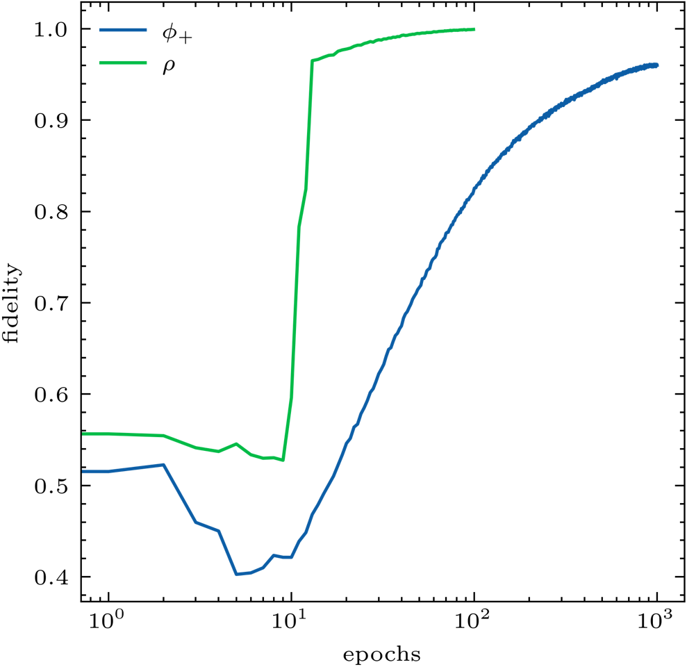
Figure 6: Learning density matrices by a stochastic state of neurons. We plot the fidelity $F(\rho,\sigma)$ by comparing the density matrix $\rho$ extracted from the expectation values and correlations of two-level neurons to a given density matrix $\sigma$ that is to be learned. The fidelity monitors the progress after a given number of training epochs. We compare two density matrices: a maximally entangled one ($\psi_{+}$) and a random one ($\rho$). The figure is taken from ref. Pehle and Wetterich (2022).

Fig. 6 demonstrates the learning of two particular density matrices Pehle and Wetterich (2022). The precision of the agreement of the matrix obtained as a result of a given number of learning steps (epochs) with the wanted density matrix is measured by the “fidelity”, a concept generally used to measure precision in quantum computations. The fidelity compares two density matrices $\rho$ and $\sigma$. It is defined by

$$F(\rho,\sigma)=\left(\mathrm{tr}\left\{\sqrt{\sqrt{\rho}\sigma\sqrt{\rho}}\right\}\right)^{2}.$$ (6.4.5)

We demonstrate the learning of the probability distribution which realizes the density matrix of the pure maximally entangled state with wave function

$$\psi_{+}=\frac{1}{\sqrt{2}}(\ket{\uparrow\uparrow}+\ket{\downarrow\downarrow}),$$ (6.4.6)

as well as the one for a randomly generated density matrix $\rho$. Both can be learned after a sufficient number of epochs, where we observe that the learning of a highly entangled state stakes somewhat longer.

Once the stochastic dynamics realizing a given density matrix has been learned, one can measure all correlations of the six Ising spins and construct the probability distribution. In Fig. 7 we display the probabilities for the $64$ configurations of the six Ising spins that result from this learning.

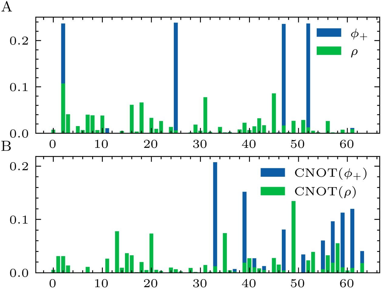
Figure 7: Classical probabilities for quantum states. In part $A$ we plot the probability distributions which are mapped to the density matrix of the maximally entangled pure state $\psi_{+}=\frac{1}{\sqrt{2}}(|00\rangle+|11\rangle)$ (blue) and for a randomly chosen density matrix (green). In part $B$ we display the probability distributions corresponding to the density matrices which are obtained from the ones of part $A$ by applying the CNOT-gate. The labels $0\dots 63$ refer to the configurations of six classical Ising spins $s_{k}^{(i)}$, $i=1,2$, $k=1\dots 3$. They can be though as binary numbers constructed from the bits associated to Ising spins. For example the label three corresponds to the spin configuration $(-1,-1,-1,-1,1,1)$. This figure demonstrates that entangled quantum states can be realized by classical probability distributions, and quantum gates by changes of these probability distributions. The figure is taken from ref. Pehle and Wetterich (2022).

We do this for both the state $\psi_{+}$ and the randomly chosen density matrix. We also perform the learning of the density matrices which obtain by applying the CNOT-gate to $\psi_{+}$ and the randomly chosen $\rho$. The result is also shown in Fig. 7. This demonstrates that the system can learn the density matrices that obtain by applying basis quantum gates to a given density matrix.

Fig. 8 displays the expectation values and correlations used for the quantum density matrix.

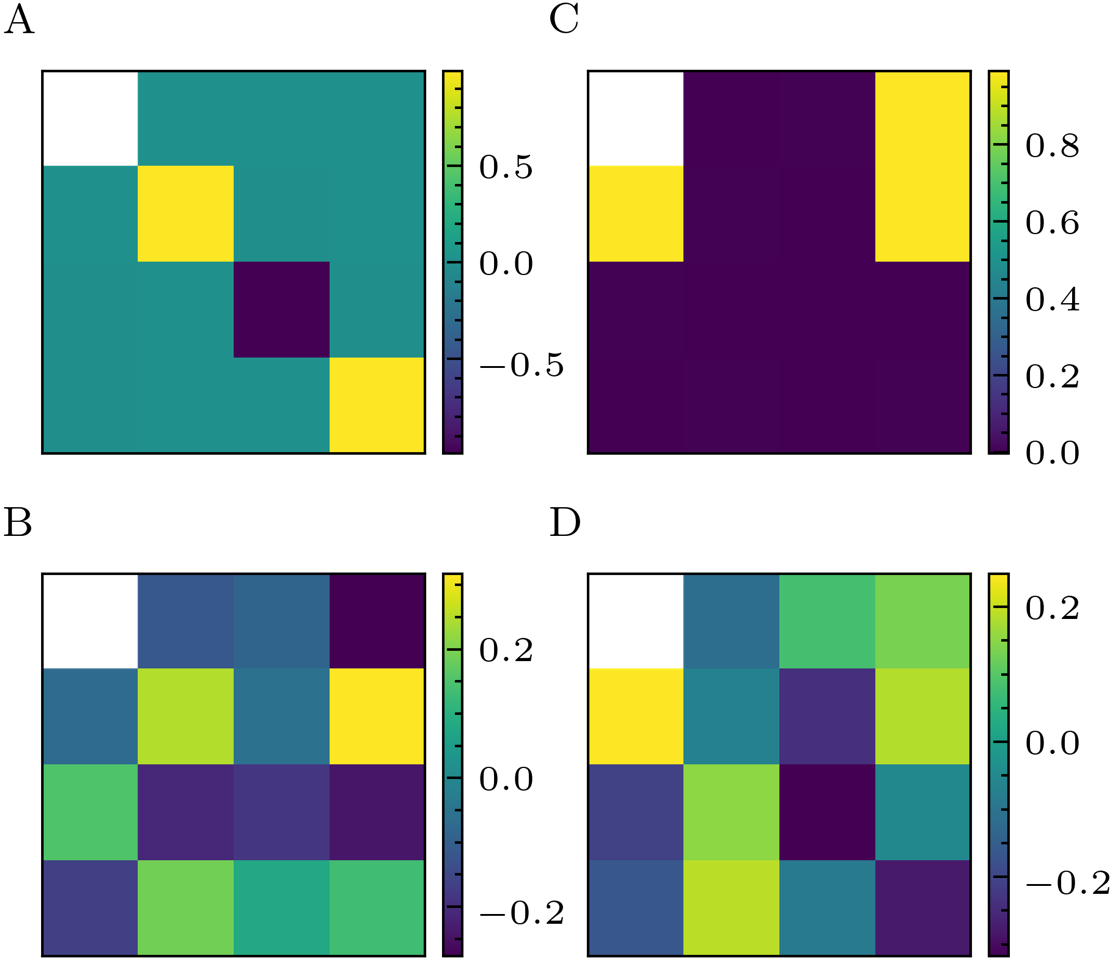
Figure 8: Expectation values and correlations of classical Ising spins which are used for the quantum density matrix. The first row indicates the three expectation values $\langle s_{k}^{(1)}\rangle$, while the first column indicates $\langle s_{k}^{(2)}\rangle$. The remaining $3\times 3$ matrices display the correlations $\langle s_{k}^{(1)}s_{k}^{(2)}\rangle$. We display the expectation values and correlations learned by the neuromorphic stochastic system for the pure entangled quantum state in part $A$, and for a randomly chosen density matrix in part $B$. The parts $C$ and $D$ display the results for density matrices that obtain from $A$ and $B$ by applying the CNOT gate. Similar results obtain by analytic computation from the probability distributions in Fig. 7. The figure is taken from ref. Pehle and Wetterich (2022).

They can directly be extracted from measurement. On the other hand, we can equivalently compute them from the classical probability distributions shown in Fig. 7. This can be used as a check that the probability distributions found are indeed correct. We emphasize that the probability distributions for the $64$ configurations realizing a given quantum density matrix are not unique. Only $15$ linear combinations of the $64$ probabilities enter the density matrix. Therefore a different training typically finds a different probability distribution for the configurations realizing a given quantum density matrix.

If the system would have to learn how to perform the basic quantum gates for arbitrary probability distributions realizing a given quantum density matrix, it has to learn how to update the parameters of the stochastic dynamics for arbitrary probability distributions realizing a given density matrix. Such a procedure would learn a large amount of redundant information. For learning a given quantum gate it is sufficient that a map between stochastic parameter sets for two consecutive time periods is learned such that the $15$ expectation values and correlations are changed according to the unitary transformation. This task is similar to the one discussed in the preceding section. The other $63-15=48$ correlations for the six Ising spins simply play no role. Together with the neurons not used for the quantum density matrix they constitute the environment for the quantum subsystem.

Already the implementation of the quantumness gate can be used to answer a computational question which is not easily accessible otherwise: Is the minimal correlation map a complete bit-quantum map or not? The answer is positive for two qubits and negative for three or more qubits. Completeness of the correlation map means that arbitrary quantum density matrices can be realized for suitable probability distributions of the classical bits. For this purpose one investigates a very large number of randomly chosen density matrices. For two qubits the learning of the associated stochastic dynamics and corresponding probability distribution has always been successful. Without being a formal proof this constitutes a rather strong argument for completeness. For three qubits we have found no successful learning for a certain class of density matrices. This is again not a formal proof of incompleteness of the minimal correlation map. In principle, it could be a shortcoming of the learning algorithm. Having the indication of incompleteness it was possible, however, to find analytically obstructions for the minimal correlation map to work for GHZ-states Pehle and Wetterich (2022).

Outlook on correlated computing

We have presented several examples for correlated computing. They are necessarily based on some type of probabilistic computing since only non-trivial probability distributions can realize the necessary correlations between two-level observables. Quantum computation by real atoms or photons implement these correlations by the very nature of quantum systems. For example, the correlations between different directions of the quantum spin, which may be regarded as independent two-level observables, follow automatically from the uncertainty relations or similar properties of the quantum formalism. In our example the two-level observables are represented by some type of classical bits, as neurons in two different possible states. Then the quantum correlations have to be prepared by the initialization through a quantumness gate. It seems very unlikely that the high precision of quantum correlations for sufficiently isolated real quantum particles can be reached by the classical spins. Also the extension to many entangled qubits is, in principle, straightforward for real quantum particles, while it is far from obvious for classical bits. This points to a clear superiority of real quantum computers as compared to realizations by classical bits.

What is then the point of our very simple correlated computers realized by classical bits? It is the demonstration that the performance of tasks by correlated computing does not need the extreme isolation of microscopic qubits. The Ising spins can be macroscopic observables, and the issue of decoherence does not seem to play an important role. This implies that correlated computing may be used in practice by nature for performing certain tasks. The evolution may have taught animals to employ correlations between the states of neurons in order to recognize patterns or to store memory. In the same way deep artificial neural networks may learn to employ correlations between different building blocks. Our simple examples demonstrate that the presence of probabilities needs not to reduce the computational power. In contrast, probabilities open the door to the use of correlations. Much more information can be stored in correlations between configurations of Ising spins than in the sharp independent configurations. And, most important, for a correlated system the manipulation of one observable can simultaneously affect many other observables as well.

7   Conditional probabilities and measurements

Probabilistic realism Wetterich is based on the concept of an overall probability distribution, describing the whole Universe from the infinite past to the infinite future. In practice, one is often interested, however, in subsystems that are local in time and space. A typical physicists question asks: If I have prepared certain initial experimental conditions, what will be the outcome? This type of questions concerns conditional probabilities.

Conditional probabilities are the key concept for understanding the outcomes of sequences of measurements. One needs the conditional probabilities $(w_{a}^{A})_{b}^{B}$ to find for an observable $A(t_{2})$ the value $a$ under the condition that another observable $B(t_{1})$ has been found previously to have the value $b$. They determine the correlations found in sequences of measurements – the measurement correlations. Conditional probabilities and measurement correlations are not unique – they depend on the details how measurements are performed. Conditional probabilities cannot be computed from the probabilistic information for a subsystem. They involve the specification of additional input on the circumstances how a sequence of two measurements for the subsystem is performed. We define criteria for ideal measurements for subsystems. For ideal measurements in typical subsystems the measurement correlations do not correspond to the classical correlations in the overall probabilistic system. This is particularly apparent for the continuum limit of time-local subsystems. The classical correlation functions depend on precise details of the environment and measurement apparatus, as well as on details of averaging procedures. They do not correspond to ideal measurements. In contrast, there exist other robust measurement correlations obeying the criteria for ideal measurements. They are based on operator products in our formalism for time-local subsystems.

We discuss the connection between ideal measurements and conditional probabilities in detail since many misconceptions for measurements in quantum mechanics arise from an insufficient consideration of conditional probabilities. In particular, the reduction of the wave function is nothing else than an appropriate formalism for the description of conditional probabilities for decoherent ideal measurements. There is no need to relate the reduction of the wave function to a non-unitary physical process or to a “many world interpretation” of quantum mechanics. We will find that for most cases the classical correlation function is not an acceptable measurement correlation for ideal measurements in subsystems. Confounding measurement correlations and classical correlations is at the root of some other “paradoxes of quantum mechanics” and “no-go theorems” that we will discuss in sect. 8.

7.1   Conditional probabilities

Conditional probabilities concern sequences of events or observations. These are typically time sequences, but not necessarily so. Consider two Ising spins $A$ and $B$. One wants to make statements about the probability for the event $A=1$, given that the event $B=1$ has happened. For a corresponding sequence of two measurements the question asks for the conditional probability $(w_{+}^{A})_{+}^{B}$ to find for $A$ the value $+1$ if $B$ is measured to be $B=1$. Similarly, the conditional probability to find $A=+1$ given that $B=-1$ is denoted by $(w_{+}^{A})_{-}^{B}$ and so on. For an Ising spin $A$ either $A=1$ or $A=-1$ has to happen independently of the outcome of the measurement of $B$, such that the conditional probabilities obey the rule

$$(w_{+}^{A})_{+}^{B}+(w_{-}^{A})_{+}^{B}=1\,,\quad(w_{+}^{A})_{-}^{B}+(w_{-}^{A})_{-}^{B}=1\,.$$ (7.1.1)

The generalization of conditional probabilities to observables with more than two possible measurement values is straightforward.

Most statements in physics concern conditional probabilities, rather than the probabilities for events $A$ or $B$. Imagine that a person holds a pen between two fingers one meter above the floor and opens the hand. A physicist would predict that after some time the probability for the pen to be on the floor in a radius of $20\,$m around this person ($A=1$) is close to one if the hand is open ($B=1$), while the probability that the pen is not on the floor at this location ($A=-1$) is almost zero. This is a statement about conditional probabilities, $(w_{+}^{A})_{+}^{B}\approx 1$, $(w_{-}^{A})_{+}^{B}\approx 0$. In contrast, from the point of view of the overall probability distribution for the whole Universe the probability for a pen to be on the floor at the given time and place $w_{+}^{A}=w(A=1)$ is almost zero. Given initial conditions at the time of the emission CMB fluctuations the pen on the floor requires 1) that a galaxy has formed in the vicinity of the position $x$ on the floor, 2) that a star with a planet is there, 3) that a civilization with pens has developed and so on. If $A=1$ is the event that there is a pen in some interval of time and space around $t$ and $x$, the probability $w(A=1)$ is extremely close to zero, in contrast to the conditional probability $(w_{+}^{A})_{+}^{B}$ which is very close to one. It is rather obvious from this simple example that the interest lies in the conditional probabilities, not in the probabilities themselves. For most practical purposes one uses conditional probabilities without naming them in this way. The condition that certain initial conditions have been prepared is not mentioned explicitly.

It is important to distinguish between the conditional probabilities $(w_{+}^{A})_{+}^{B}$ and the probabilities $w_{++}^{(AB)}$ to find the events $A=1$, $B=1$ in the overall probabilistic system. The probability $w_{++}^{(AB)}$ to find a sequence $B=1$, $A=1$ can be expressed as the product of the probability for the event $B=1$ and the conditional probability to find $A=1$ for $B=1$ given

$$w_{++}^{(AB)}=(w_{+}^{A})_{+}^{B}w(B=1)=(w_{+}^{A})_{+}^{B}w_{+}^{B}\,.$$ (7.1.2)

While both $w(B=1)=w_{+}^{B}$ and $w_{++}^{(AB)}$ may be very small, the conditional probability $(w_{+}^{A})_{+}^{B}$ can be large. This is precisely what happens in our example with the pen. From the point of view of the whole Universe the probability for a hand with a pen opening at $t_{1}$ and $x_{1}$, e.g. $w(B=1)$, is tiny. Also the probability $w_{++}^{(AB)}$ for the two events, a hand with a pen opening at ($t_{1},x_{1}$), ($B=1$), and a pen at ($t_{2},x_{2}$), ($A=1$), is extremely small. Nevertheless, the conditional probability, given formally by

$$(w_{+}^{A})_{+}^{B}=\frac{w_{++}^{(AB)}}{w_{+}^{B}}\,,$$ (7.1.3)

is close to one. We note that conditional probabilities can be determined by eq. (7.1.3) for arbitrarily small non-zero $w_{+}^{B}$. Eq. (7.1.3) is not meaningful, however, if the probability for the event $B=1$ is precisely zero, e.g. $w_{+}^{B}=w_{++}^{(AB)}=w_{-+}^{(AB)}=0$.

In the following we will often forget about the overall probabilistic system and rather concentrate on subsystems as quantum systems prepared by some experimental conditions. The importance of conditional probabilities for sequences of measurements does not change. Only the probabilistic information of the subsystem replaces the overall probability distribution. We will denote in this case by $w_{+}^{A}$ the probability to find the value $+1$ for the observable $A$, as computed from the probabilistic information of the subsystem. The meaning and notation of conditional probabilities remains the same as before.

Let us consider subsystems with incomplete statistics, where $A$ and $B$ are system observables but the classical correlation function $\braket{AB}_{\text{cl}}$ is not available. The probabilistic information of the subsystem permits the computation of $w_{\pm}^{A}$ and $w_{\pm}^{B}$, but provides no direct prescription how to compute $w_{++}^{(AB)}$ etc. At this stage neither $w_{++}^{(AB)}$ nor the conditional probability $(w_{+}^{A})_{+}^{B}$ is fixed. For subsystems with incomplete statistics one needs some type of independent information that defines the conditional probabilities. In other words, the conditional probabilities are not simply properties of the probabilistic information of the subsystem. They need additional input how a sequence of measurements of $A$ and $B$ is done. This will lead us to the concept of ideal measurements.

7.2   Sequence of measurements

A conceptual understanding of measurements is a rather complex issue. From the point of view of the overall probabilistic description of the world, measurements and the humans or apparatus performing them are part of the world and included in the overall probability distribution. We do not aim here for a systematic discussion of the measurement process. We rather highlight a few aspects Wetterich (2009) that are crucial for the conceptual understanding of a “classical” probabilistic description.

In particular, we emphasize that the correlations found in sequences of measurements are not unique. They depend on the precise way how measurements are performed. Correspondingly, there are many different product structures of observables that correspond to sequences of measurements. In general, they do not correspond to the “classical product” of observables, which is often not available for a subsystem. The products of observables relevant for measurements are often non-commutative. The order in a sequence of measurement matters.

Different types of measurements

Every student in physics learns that the outcome of a measurement or a sequence of measurements depends on how the measurement is done. There are good measurements that provide valuable information about a system, and other measurements that depend on rather random circumstances of the environment of a system. In the case of two Ising spins or yes/no decisions $A$ and $B$, every sequence of first measuring $B$ and subsequently $A$ will give one of the four possible results ($++$), ($+-$), ($-+$), ($--$). Imagine a physics class where each student should perform the sequence of measurements of $A$ and $B$ with his own constructed apparatus. An experienced researcher may be able to estimate the outcomes of the different measurement devices. She may concentrate on the measurements where the first measurement has found $B=1$. Knowing the physics law behind the experiment, she predicts that an ideally constructed apparatus will find $A=1$. For this ideal apparatus the conditional probability is $(w_{+}^{A})_{+}^{B}=1$. For some other apparatus she may judge that the outcome will be random $(w_{+}^{A})_{+}^{B}=(w_{-}^{A})_{+}^{B}=1/2$. And still for others there will be conditional probabilities in between.

The lesson from this simple example is that conditional probabilities for a sequence of measurements depend on how the measurement is done. The conditional probabilities do actually not depend on the judgement of the experienced researcher. In view of a probabilistic description of the whole process they are properties of the measurement apparatus employed. Only for an ideal measurement apparatus one has a conditional probability, $(w_{+}^{A})_{+}^{B}=1$, independently if this has been recognized by the experienced researcher or not.

Measurement correlation

Depending on the precise way how a measurement is done one will find different “measurement correlations”. For the two observables $A$ and $B$ the outcomes depend on the conditional probabilities. Those depend, in turn, on the way how the measurements are done. A basic rule for measurements associates the probabilities $w^{(AB)}$ for the outcome of a sequence to the conditional probabilities and the probabilities to find a given value for the first measurement,

$$w_{++}^{(AB)} =(w_{+}^{A})_{+}^{B}w_{+}^{B}\,,\quad w_{+-}^{(AB)}=(w_{+}^{A})_{-}^{B}w_{-}^{B}\,,$$

$$w_{-+}^{(AB)} =(w_{-}^{A})_{+}^{B}w_{+}^{B}\,,\quad w_{--}^{(AB)}=(w_{-}^{A})_{-}^{B}w_{-}^{B}\,.$$ (7.2.1)

This can be used in order to define the measurement correlation

$$\braket{AB}_{m}=w_{++}^{(AB)}+w_{--}^{(AB)}-w_{+-}^{(AB)}-w_{-+}^{(AB)}\,.$$ (7.2.2)

The measurement correlation is not a universal quantity. It depends on how the measurement is done, as expressed by the conditional probabilities. In general, the measurement correlation is not the classical correlation function or any other universally defined correlation function. It always involves the particular realisation of a measurement by a given apparatus or observation.

By using the same symbol $w_{++}^{(AB)}$ for the probability of a sequence of events in some time- and space-local subsystem as the one used for the overall probability distribution of the Universe in eq. (7.1.2) we follow a commonly used procedure. We treat the subsystem as if it would be the whole Universe and take it for this particular purpose as a replacement of the overall probabilistic system. From the point of view of the whole Universe $w_{++}^{(AB)}$ is related to some sort of conditional probability, namely under the condition that a suitable subsystem is realized. This condition is here tacitly assumed, and the context makes the meaning of $w_{++}^{(AB)}$ clear.

Still, the time- and space-local subsystem associated to the new overall system can be much larger than the subsystem actually employed for the description of the sequence of measurements. It may contain an environment which may influence the outcome of the sequence of measurements. Typically, the precise details of the measurement apparatus are part of this environment. The subsystem for $A$ and $B$ does not include the probabilistic information related to these details. Subsystems occur here on different levels. For example, the quantum subsystem for the observables $A$ and $B$ is a subsystem of the experiment-subsystem which includes the measurement apparatus. This in turn is a subsystem of the overall probabilistic system. We also deal with classical statistical subsystems of the overall probabilistic system, which have in turn quantum systems as subsystems.

Different products of observables for different
measurements

Within the subsystem with observables $A$ and $B$ one can formally define a product of the two observables $(A\circ B)_{m}$ such that its expectation value is the measurement correlation,

$$\braket{(A\circ B)_{m}}=\braket{AB}_{m}\,.$$ (7.2.3)

Indeed, for any given apparatus the sequence of measurements of $A$ and $B$ is a new combined observable with possible measurement values $\pm 1$. Different types of apparatus correspond to different products $(A\circ B)_{m}$. We conclude that for subsystems the product of two observables is not unique. There exist many different definitions of observable products $C=(A\circ B)_{m}$, since there are many different ways to perform measurements. The classical observable product in the overall probabilistic system, $C_{\tau}=A_{\tau}B_{\tau}$, is only one out of many possibilities. We will see that for many subsystems, in particular for subsystems with incomplete statistics, it plays no role.

The product $A\circ B$ is, in general, not commutative. The order in the sequence of two measurements can matter. It makes a difference if $A$ or $B$ are measured first. Thus the measurement correlation can depend on the order of the two factors

$$\braket{AB}_{m}\neq\braket{BA}_{m}\,,$$ (7.2.4)

in distinction to the classical correlation. This can be seen by the different expressions in terms of the conditional probabilities

$$\braket{BA}_{m}=w_{++}^{(BA)}+w_{--}^{(BA)}-w_{+-}^{(BA)}-w_{-+}^{(BA)}\,,$$ (7.2.5)

where

$$w_{++}^{(BA)} =(w_{+}^{B})_{+}^{A}w_{+}^{A}\,,\quad w_{+-}^{(BA)}=(w_{+}^{B})_{-}^{A}w_{-}^{A}\,,$$

$$w_{-+}^{(BA)} =(w_{-}^{B})_{+}^{A}w_{+}^{A}\,,\quad w_{--}^{(BA)}=(w_{-}^{B})_{-}^{A}w_{-}^{A}\,.$$ (7.2.6)

There is no a priori direct relation between $w^{(AB)}$ in eq. (7.2) and $w^{(BA)}$ in eq. (7.2). One has to find this relation for each concrete sequence of two measurements.

The expectation value of the observable that is measured first does not depend on the conditional probabilities for the sequence of measurements. Measuring first $B(t_{1})$ one has

$$\braket{B(t_{1})}=\braket{B}=w_{+}^{B}-w_{-}^{B}\,,$$ (7.2.7)

where the probabilities $w_{\pm}^{B}$ to find $B=\pm 1$ are part of the probabilistic information of the subsystem. For the expectation value of the second observable $A(t_{2})$ the way how the measurement is performed matters, however. Indeed, $\braket{A(t_{2})}$ involves the conditional probabilities

$$\braket{A(t_{2})}_{B}=\braket{A}_{B}=w_{++}^{(AB)}+w_{--}^{(AB)}-w_{+-}^{(AB)}-w_{-+}^{(AB)}\\ =\left[(w_{+}^{A})_{+}^{B}-(w_{-}^{A})_{+}^{B}\right]w_{+}^{B}+\left[(w_{+}^{A})_{-}^{B}-(w_{-}^{A})_{-}^{B}\right]w_{-}^{B}\,.$$ (7.2.8)

Performing first a measurement of $B(t_{1})$ can influence the expectation value for $A(t_{2})$. The expectation value $\braket{A(t_{2})}_{B}$ can differ from the expectation value obtained without the measurement of $B$, i.e.

$$\braket{A(t_{2})}=w_{+}^{A}-w_{-}^{A}\,.$$ (7.2.9)

The expectation value (7.2.9) describes a measurement in the subsystem which evolves without any disturbance. In contrast, $\braket{A}_{B}$ in eq. (7.2.8) takes into account that the subsystem may be influenced by the measurement of $B(t_{1})$. The measurement brings a subsystem into contact with its environment. A closed subsystem follows its evolution law, as formulated in terms of the probabilistic information for the subsystem, only for the time between measurements. The interaction with the environment due to the measurement of $B$ at $t_{1}$ can influence the state of the subsystem at $t_{1}$, which serves as initial condition for the evolution at $t>t_{1}$. It is this influence that is responsible for a possible difference between $\braket{A(t_{2})}_{B}$ and $\braket{A(t_{2})}$.

Conditional probabilities from measurement
correlations

The relation between the conditional probabilities and the measurement correlation can be inverted. Whenever $\braket{AB}_{m}$, $\braket{A}_{B}$ and $\braket{B}$ are known, one can reconstruct the conditional probabilities if they are defined. With

$$w_{\pm}^{B}=\frac{1}{2}\left(1\pm\braket{B}\right)$$ (7.2.10)

and

$$w_{++}^{(AB)}=\frac{1}{4}(1+\braket{A}_{B}+\braket{B}+\braket{AB}_{m})\,,$$

$$w_{+-}^{(AB)}=\frac{1}{4}(1+\braket{A}_{B}-\braket{B}-\braket{AB}_{m})\,,$$

$$w_{-+}^{(AB)}=\frac{1}{4}(1-\braket{A}_{B}+\braket{B}-\braket{AB}_{m})\,,$$

$$w_{--}^{(AB)}=\frac{1}{4}(1-\braket{A}_{B}-\braket{B}+\braket{AB}_{m})\,,$$

the conditional probabilities obtain by inverting the relations (7.2). For the system of two Ising spins we observe a one to one correspondence between the measurement correlation and expectation values $\braket{B}$, $\braket{A}_{B}$ on one side and the conditional probabilities on the other side.

7.3   Ideal measurements for subsystems

Not all measurements are equivalent – some are better than others. Physicists have developed the concept of “ideal measurements” in order to find out the properties of subsystems. An ideal measurement apparatus is one that is best suited to measure the properties of the subsystem rather than its environment. The concept of an ideal measurement may single out a particular set of conditional probabilities or a particular measurement correlation among the many possibilities. In turn, it may single out a specific ideal observable product $A\circ B$ among the many possible choices of products $(A\circ B)_{m}$. (If we discuss ideal measurements we often will omit the subscript $m$ for measurement.)

Ideal measurements should be as insensitive as possible to the state of the environment of a subsystem, and we develop criteria for this property. An important finding is that the measurement correlations for ideal measurements are not given by the classical correlation function. We distinguish between coherent and decoherent ideal measurements. For the particular case of quantum subsystems we discuss in detail the different outcomes for correlation functions for these two types of ideal measurements. For coherent ideal measurements the measurement correlation is the quantum correlation as defined by the product of Heisenberg operators. For decoherent ideal measurements the state of the quantum subsystem is influenced by the interaction with the environment during the measurement process. This is related to the “reduction of the wave function”.

Criteria for ideal measurements

Ideal measurements for subsystems should obey five criteria:

1. Measurement of subsystems properties

   The measurement should measure properties of the subsystem, not of its environment. The outcome of a given ideal measurement should only depend on the probabilistic information of the subsystem. This means that the conditional probabilities and the measurement correlation should be computable from the variables characterizing the subsystem.

2. Independence of environment

   In other words, the outcome of an ideal measurement for a subsystem should not depend on the state of its environment. This is a type of “common sense criterion” that is used in practice. The influence of the state of the environment is considered as “noise” which has to be minimized for an ideal measurement. The criterion 2 does not state that the environment plays no role for the measurement. Only the outcome of the measurement should not depend on the particular state of the environment.

   Typically, the measurement apparatus is part of the environment of a subsystem. The measurement process necessarily involves an interaction between the subsystem and the measurement apparatus, and therefore an interaction between the subsystem and its environment. Nevertheless, ideal measurements should not introduce additional probabilistic information from the environment into the subsystem, or at least should restrict such additional information to a minimum. Despite the interaction with the environment during the measurement process and a possible change of state of the subsystem induced by this interaction, the outcome of the sequences of ideal measurements should not depend on the state of the measurement apparatus. A possible change of state of the subsystem during the measurement process should be computable from the probabilistic information of the subsystem.

3. Non-intrusiveness

   The outcome of a sequence of ideal measurements should be computable with the time evolution of the subsystem between two measurements. We distinguish coherent and decoherent ideal measurements. For coherent ideal measurements the first measurement of $B(t_{1})$ should not alter the subsystem. The probabilistic information of the subsystem after the measurement is the same as before the measurement. This implies, in particular, that $\braket{A(t_{2})}$ is the same with or without the measurement of $B(t_{1})$. If the probabilistic information in a subsystem is sufficient to compute for two probabilistic observables $A(t_{2})$ and $B(t_{1})$ the expectation value $\braket{A(t_{2})B(t_{1})}$, $t_{2}>t_{1}$, this correlation should coincide with the measurement correlation for coherent ideal measurements. For probabilistic observables $\braket{A(t_{2})B(t_{1})}$ often differs from the classical correlation function.

   For “decoherent ideal measurements” the measurement of $B(t_{1})$ may change the state of the subsystem. This change should be computable from the probabilistic information of the subsystem. The non-intrusiveness of the measurement procedure is now limited to the time inbetween measurements.

4. Repetition of identical measurements

   If the second observable $A(t_{2})$ is identical to $B(t_{1})$ and $t_{2}\to t_{1}$, one measures twice the observable $B(t_{1})$. If the first measurement finds the value $b_{m}$, the second measurement should find this value again. In the continuum limit for time this property should hold if $|t_{2}-t_{1}|$ is much smaller than the characteristic time for the evolution of the subsystem.

5. Compatibility with equivalence classes

   Probabilistic observables for a subsystem correspond to equivalence classes of observables of the overall probabilistic system. Many different observables of the overall system are mapped to the same probabilistic observable of the subsystem. They form an equivalence class of observables. From the point of view of the subsystem the differences between overall observables belonging to the same equivalence class should be regarded as properties of the environment. Ideal measurements in a subsystem should be compatible with the notion of the equivalence class. The outcome should only depend on the equivalence class, not on the specific member. If two observables $A$ and $A^{\prime}$ belong to the same equivalence class they may still be different observables in the overall system. This difference concerns properties of the environment of the subsystem. Ideal measurements in a subsystem should not be sensitive to this difference. The outcome should be the same for all members of a given equivalence class.

The five criteria are not independent. They reflect different facets of the basic requirement that any ideal measurement in a subsystem should be as independent as possible from the state of the environment.

Time-local subsystem

For an understanding of time-sequences of measurements we employ the time-local subsystem as a crucial concept. It is characterized by the probabilistic information at a given time $t$. Time-local subsystems can be defined for every overall probabilistic system for all events in time and space. They are discussed in detail in ref. Wetterich . We summarize here the results relevant for measurement sequences.

By integrating in the overall probability distribution over the probabilities for all configurations in the past, $t^{\prime}<t$, and focusing on a given configuration $\tau$ at $t$, one obtains the classical wave function $\tilde{q}(t)$ with components $\tilde{q}_{\tau}(t)$. The wave function $\tilde{q}(t+\varepsilon)$ at the next time step is determined by a linear evolution law involving the step evolution operator $\hat{S}(t)$,

$$\tilde{q}_{\tau}(t+\varepsilon)=\hat{S}_{\tau\rho}(t)\tilde{q}_{\rho}(t)\,.$$ (7.3.1)

Similarly, integrating out the future, $t^{\prime}>t$, yields the conjugate wave function $\bar{q}(t)$. We concentrate here on orthogonal step evolution operators $\hat{S}(t)$. In this case one can identify $\bar{q}(t)=\tilde{q}(t)=q(t)$, once one factors out an overall transition amplitude Wetterich . The time-local classical probabilities $p_{\tau}(t)$ are then given by the square of the components of the classical wave function

$$p_{\tau}(t)=q_{\tau}^{2}(t)\,.$$ (7.3.2)

For probabilistic automata we recover the setting of sect. 2.2. The classical wave function is a probability amplitude. In contrast to the general case for local probabilities it obeys a linear evolution law (7.3.1). As compared to the probabilities the classical wave function contains some redundancy, namely the signs of $q_{\tau}(t)$. The corresponding local $\mathbb{Z}_{2}$ gauge symmetry can be fixed by choosing a sign convention for $q_{\tau}(t)$. Due to the linear evolution law and the possibility of basis changes familiar from quantum mechanics the classical wave function is more suitable for the understanding of the time evolution than the classical time-local probability distribution.

The classical density matrix $\rho^{\prime}(t)$ is a bilinear of the wave function

$$\rho^{\prime}_{\tau\rho}(t)=q_{\tau}(t)q_{\rho}(t)\,.$$ (7.3.3)

It contains more time-local probabilistic information than the probabilities which are given by its diagonal elements, $p_{\tau}(t)=\rho_{\tau\tau}(t)$. It obeys again a linear evolution law, $\hat{S}^{-1}(t)=\hat{S}^{T}(t)$,

$$\rho^{\prime}(t+\varepsilon)=\hat{S}(t)\rho^{\prime}(t)\hat{S}^{-1}(t)\,.$$ (7.3.4)

This can be extended to an arbitrary time $t_{1}>t$

$$\rho^{\prime}(t_{1})=U(t_{1},t)\rho^{\prime}(t)U^{-1}(t_{1},t)\,,$$ (7.3.5)

with

$$U(t_{1},t)=\hat{S}(t_{1}-\varepsilon)\hat{S}(t_{1}-2\varepsilon)\dots\hat{S}(t+\varepsilon)\hat{S}(t)\,.$$ (7.3.6)

For a time-local classical observable $A(t)$ the possible measurement values $A_{\tau}(t)$ depend only on the configuration $\tau$ at $t$. Its expectation value obeys

$$\langle A(t)\rangle=\sum_{\tau}p_{\tau}(t)A_{\tau}(t)=\mathrm{tr}\big{\{}\rho^{\prime}(t)\hat{A}(t)\big{\}}\,,$$ (7.3.7)

with diagonal operator $\hat{A}_{\tau\rho}(t)=A_{\tau}(t)\delta_{\tau\rho}$. This generalizes eq. (2.2.5). The probabilistic information of the density matrix at $t$ is sufficient for a computation of the expectation value of a time-local classical observable at $t_{1}$ different from $t$,

$$\langle A(t_{1})\rangle= \mathrm{tr}\big{\{}\hat{A}(t_{1})\rho^{\prime}(t_{1})\big{\}}$$

$$= \mathrm{tr}\big{\{}\hat{A}(t_{1})U(t_{1},t)\rho^{\prime}(t)U^{-1}(t_{1},t)\big{\}}$$

$$= \mathrm{tr}\big{\{}\hat{A}_{H}(t_{1},t)\rho^{\prime}(t)\big{\}}\,,$$ (7.3.8)

where we introduce the Heisenberg operator

$$\hat{A}_{H}(t_{1},t)=U(t,t_{1})\hat{A}(t_{1})U(t_{1},t)\,.$$ (7.3.9)

With

$$U(t,t_{1})=U^{-1}(t_{1},t)\,,\quad U(t,t)=1\,,$$ (7.3.10)

the relation (7.3) is valid for arbitrary $t_{1}$.

Let us consider next two time-local classical observables $A(t_{2})$ and $B(t_{1})$. Their classical correlation function $\langle A(t_{2})B(t_{1})\rangle_{\text{cl}}$ can be computed from the overall probability distribution. Equivalently it can be expressed in terms of the time ordered product of Heisenberg operators

$$\langle A(t_{2})B(t_{1})\rangle_{\text{cl}}=\mathrm{tr}\big{\{}\rho^{\prime}(t)T\{\hat{A}_{H}(t_{2},t)\hat{B}_{H}(t_{1},t)\}\big{\}}\,,$$ (7.3.11)

with

$$T\{\hat{A}_{H}(t_{2},t)\hat{B}_{H}(t_{1},t)\}=\begin{cases}\hat{A}_{H}(t_{2},t)\hat{B}(t_{1},t)\ \text{for}\ t_{2}>t_{1}\\ \hat{B}_{H}(t_{1},t)\hat{A}_{H}(t_{2},t)\ \text{for}\ t_{2}<t_{1}\,.\end{cases}$$ (7.3.12)

The time ordering is important since in general the operators $\hat{A}_{H}(t_{2},t)$ and $\hat{B}(t_{1},t)$ do not commute. The time ordered product is commutative, as appropriate for the classical correlation function. We will see that it is precisely this time ordering that makes the classical correlation inappropriate for a measurement correlation in the continuum limit.

Coherent ideal measurements

The measurement correlation depends on the type of local observables. For the sake of simplicity we focus on two-level observables $A,B$. The simplest case are Ising spins at neighboring sites, as $A=s(t_{2}),B=s(t_{1}),t_{2}>t_{1}$. In this case the expectation value $\braket{AB}$ can be computed from the probabilistic information of the subsystem. For coherent ideal measurements one has according to the criterion 3

$$\braket{AB}_{m}=\braket{s(t_{2})s(t_{1})}=\mathrm{tr}\left\{\rho^{\prime}(t)\hat{A}_{H}(t_{2},t)\hat{B}_{H}(t_{1},t)\right\}\,,$$ (7.3.13)

with $\hat{A}_{H}(t_{2},t)$ and $\hat{B}_{H}(t_{1},t)$ the Heisenberg operators associated to $A=s(t_{2})$ and $B=s(t_{1})$. The density matrix $\rho^{\prime}$ and Heisenberg operators for observables are defined for the time-local “classical” probabilistic subsystem. Since $\rho^{\prime}$ is a symmetric matrix only the symmetric part of the operator product $\hat{A}_{H}(t_{2})\hat{B}_{H}(t_{1})$ contributes to $\langle AB\rangle_{m}$. We may therefore use equivalently an expression in terms of the anticommutator $\{\hat{A}_{H},\hat{B}_{H}\}$,

$$\langle AB\rangle_{m}=\frac{1}{2}\mathrm{tr}\Big{(}\rho^{\prime}(t)\{\hat{A}_{H}(t_{2},t),\hat{B}_{H}(t_{1},t)\}\Big{)}\,,$$ (7.3.14)

where we employ that $\hat{A}_{H}$ and $\hat{B}_{H}$ are symmetric matrices for orthogonal $\hat{S}$ and $U$.

The expectation value

$$\braket{A(t_{2})}=\mathrm{tr}\left\{\rho^{\prime}(t)\hat{A}_{H}(t_{2},t)\right\}\,,$$ (7.3.15)

is the same if $B$ is measured or not. The conditional probabilities can be inferred from this measurement correlation and the expectation values $\braket{A(t_{2})}$ and $\braket{B(t_{1})}$ according to eq. (7.2), (7.2). For this particular case the measurement correlation (7.3.13) coincides with the classical correlation in the overall probabilistic system Wetterich .

The prescription for ideal coherent measurements by Heisenberg operators (7.3.13) can be extended to arbitrary observables $A(t_{2})$ and $B(t_{1})$. This formulation in terms of the Heisenberg operators $\hat{A}_{H},\hat{B}_{H}$ is compatible with the notion of equivalence classes. Two members of a given equivalence class are mapped to the same Heisenberg operator. By the criterion 4 the same measurement correlation should hold for all local probabilistic observables $A^{\prime}$ and $B^{\prime}$ that are represented by the operators $\hat{A}_{H}$ and $\hat{B}_{H}$, respectively. As we have discussed in ref. Wetterich , the classical correlations in the overall probabilistic system often differ for different representatives in the same equivalence class. Thus the relation (7.3.13) for the measurement correlation implies that, in general, the measurement correlation differs from the classical correlation. The robust object that respects the equivalence class is an observable product $A\circ B$ based on the operator product $\hat{A}_{H}\hat{B}_{H}$. It is typically non-commutative.

Continuum limit in time

These more formal considerations become particularly relevant for the continuum limit in time. We will argue that in this limit the classical correlation function based on the time-ordered operator product is no longer compatible with the criteria for ideal measurements. The reason is a clash between time ordering and time averaging. In contrast, the operator product without time ordering remains compatible with an ideal measurement.

In the continuum limit the relevant observables typically involve an averaging over infinitesimal time steps. In ref. Wetterich we have introduced a time-averaged spin observable

$$\sigma(\bar{t})=\sum_{t^{\prime}}a^{(\sigma)}(\bar{t}+t^{\prime})s(\bar{t}+t^{\prime})\,,$$ (7.3.16)

with averaging function $a^{(\sigma)}$ taking a suitable shape such that only some time-region around $\bar{t}$ contributes effectively to the averaged spin. Since $\sigma(\bar{t})$ is linear in the spins $s(\bar{t}+t’)$ we can introduce the associated Heisenberg operator

$$\hat{\sigma}_{H}(\bar{t},t)=\sum_{t^{\prime}}a^{(\sigma)}(\bar{t}+t^{\prime})U(t,\bar{t}+t^{\prime})\hat{s}(\bar{t}+t^{\prime})U(\bar{t}+t^{\prime},t)$$ (7.3.17)

and compute the expectation value as

$$\langle\sigma(\bar{t})\rangle=\mathrm{tr}\big{\{}\rho^{\prime}(t)\hat{\sigma}_{H}(\bar{t},t)\big{\}}\,.$$ (7.3.18)

There is a large family of different averaging functions $a^{(\sigma)}$ which lead to the same Heisenberg operator $\hat{\sigma}_{H}(\bar{t},t)$. If this difference cannot be resolved in the continuum limit for time the corresponding average observables $\sigma(\bar{t})$ for this family should be considered as equivalent.

One can define a possible correlation function for $t_{2}>t_{1}$ as

$$\braket{\sigma(t_{2})\sigma(t_{1})}=\mathrm{tr}\left\{\rho^{\prime}(t)\hat{\sigma}_{H}(t_{2},t)\hat{\sigma}_{H}(t_{1},t)\right\}\,.$$ (7.3.19)

This is a good candidate for the measurement correlation for coherent ideal measurements in the subsystem. It respects the structure of equivalence classes, is compatible with the time evolution of the subsystem and only uses the probabilistic information in the subsystem as encoded in the classical density matrix $\rho^{\prime}(t)$.

The correlation (7.3.19) is, in general, no longer a classical correlation function. The classical correlation function for $\sigma(t_{2})\sigma(t_{1})$ involves in eq. (7.3.19) the time ordered operator $\operatorname{T}\left\{\hat{\sigma}_{H}(t_{2},t)\hat{\sigma}_{H}(t_{1},t)\right\}$ instead of the product $\hat{\sigma}_{H}(t_{2},t)\hat{\sigma}_{H}(t_{1},t)$. The two expressions only coincide if $t_{2}-t_{1}$ is sufficiently large as compared to the interval used for the averaging $\Delta t$, and the Heisenberg operators $\hat{s}_{H}(t_{2}+t^{\prime},t)$ and $\hat{s}_{H}(t_{1}+t^{\prime},t)$ in the definition of $\hat{\sigma}_{H}(t_{2},t)$ and $\hat{\sigma}_{H}(t_{1},t)$ have no overlapping time region. Whenever $t_{2}-t_{1}$ becomes of the order $\Delta t$ or smaller the time ordered product becomes very complicated. It involves microscopic details not available in the continuum limit. It does not respect the notion of equivalence classes since different average procedures that lead to the same operators $\hat{\sigma}_{H}(t_{2},t)$ or $\hat{\sigma}_{H}(t_{1},t)$ do not yield the same time ordered products. Furthermore, no simple time evolution law exists for the time ordered product.

We conclude that the classical correlation function is not suitable for the measurement correlation for ideal measurements in the classical time-local subsystem. We generalize these findings by postulating that for two local observables $A(t_{2}),B(t_{1}),t_{2}>t_{1}$ the measurement correlation for coherent ideal measurements is given by

$$\braket{A(t_{2})B(t_{1})}_{m}=\mathrm{tr}\left\{\rho^{\prime}(t)\hat{A}_{H}(t_{2},t)\hat{B}_{H}(t_{1},t)\right\}\,.$$ (7.3.20)

Here $\hat{A}_{H}(t_{2},t)$ and $\hat{B}_{H}(t_{1},t)$ are the Heisenberg operators associated to $A(t_{2})$ and $B(t_{1})$. This measurement correlation obeys all criteria for ideal measurements in a subsystem. It equals suitable classical correlation functions in certain limiting cases, but is a much more robust object. If $A(t_{2})$ and $B(t_{1})$ are two-level observables, the measurement correlation fixes the conditional probabilities for ideal measurements. For more general cases also higher order measurement correlations will be needed for the determination of the conditional probabilities.

The measurement correlation (7.3.20) in terms of the operator product does not employ particular properties of quantum subsystems. It holds for all local-time subsystems, both for quantum systems and more general probabilistic subsystems. The central motivation arises from the continuum limit for the time-local subsystem. Still, the measurement correlation (7.3.20) remains a postulate for coherent ideal measurements. This is necessarily so and there is no direct way to derive conditional probabilities from the probability distribution of the subsystem or overall system. One has to define what is an ideal measurement – this is done in the form of a postulate for measurement correlations. There may be other possible definitions for ideal measurements in time-local subsystems. What should be clear at this stage is that the classical correlation function is not a viable candidate.

It is not always guaranteed that a measurement process exists which leaves the probabilistic information of the time-local subsystem the same before and after the measurement of $B(t_{1})$. If not, we will have to deal with decoherent ideal measurements. We will discuss below such decoherent ideal measurements for quantum subsystems, which are particular local-time subsystems. At the end it remains an experimental question if a measurement apparatus can be constructed whose results come close to coherent ideal measurements.

Quantum subsystems and quantum correlation

Quantum subsystems are time-local subsystems with incomplete statistics. We may therefore try to take over the measurement correlation (7.3.20) for coherent ideal measurements in time-local subsystems and employ the quantum correlation $\langle AB\rangle_{q}$,

$$\braket{A(t_{2})B(t_{1})}_{q}=\mathrm{tr}\left\{\rho(t)\hat{A}_{H}(t_{2},t)\hat{B}_{H}(t_{1},t)\right\}\,.$$ (7.3.21)

Here $\hat{A}_{H}(t_{2},t)$ and $\hat{B}_{H}(t_{1},t)$ are the Heisenberg operators in the quantum subsystem associated to the observables $A(t_{2})$ and $B(t_{1})$. In the real formulation $U(t_{2},t_{1})$ is an orthogonal matrix and the density matrix $\rho^{\prime}$ is symmetric. In the presence of a complex structure the density matrix $\rho$ becomes a Hermitian complex matrix, and the evolution operators $U(t_{2},t_{1})$ are unitary matrices. As a result the quantum correlation has an imaginary part if the operators $\hat{A}_{H}(t_{2})$ and $\hat{B}_{H}(t_{1})$ do not commute. For a real measurement correlation for coherent ideal measurements we propose to use the anticommutator

$$\langle A(t_{2})B(t_{1})\rangle_{m}=\frac{1}{2}\mathrm{tr}\Big{(}\rho(t)\{\hat{A}_{H}(t_{2}),\hat{B}_{H}(t_{1})\}\Big{)}\,,$$ (7.3.22)

similar to eq. (7.3.14) for the real formulation. This correlation is compatible with the notion of equivalence classes of observables and therefore robust. It obeys all criteria for ideal measurements. Translated to the real formulation of quantum mechanics it is equivalent to eq. (7.3.13). Combining the measurement correlation (7.3.22) with the expectation value as

$$\braket{A(t_{2})}=\mathrm{tr}\left\{\hat{A}_{H}(t_{2},t)\rho(t)\right\}\,,$$ (7.3.23)

one can extract the conditional probabilities for coherent ideal measurements of two-level observables from eq. (7.2). The conditional probabilities for coherent ideal measurements can also be obtained directly from a suitable projection of $\rho$ Wetterich (2009).

Decoherent ideal measurements

Not all ideal measurements in quantum subsystems are coherent ideal measurements. Often a measurement apparatus cannot preserve the coherence of the quantum information. For this case we define the notion of decoherent ideal measurements. Bell-type experiments typically assume coherent ideal measurements, while sequences of Stern-Gerlach type experiments employ decoherent ideal measurements.

We discuss the concept of decoherent ideal measurements for one qubit quantum mechanics with $A(t_{2})$ and $B(t_{1})$ having possible measurement values $\pm 1$. For a decoherent ideal measurement the measurement of $B(t_{1})$ can change the state of the subsystem. Let us work in a basis where $\hat{B}_{H}(t_{1},t_{1})$ is diagonal, $\hat{B}_{H}(t_{1},t_{1})=\tau_{3}$. The complex density matrix $\rho(t_{1})$ takes the general form

$$\rho(t_{1})=\begin{pmatrix}w_{+}^{B}&c\\ c^{*}&w_{-}^{B}\end{pmatrix},$$ (7.3.24)

with $w_{\pm}^{B}$ the probabilities to find $B=\pm 1$ and

$$\braket{B(t_{1})} =\mathrm{tr}\left\{\rho(t_{1})\hat{B}_{H}(t_{1},t_{1})\right\}=\mathrm{tr}\left\{\rho(t_{1})\tau_{3}\right\}$$

$$=w_{+}^{B}-w_{-}^{B}\,.$$ (7.3.25)

For a pure state one has $|c|^{2}=w_{+}^{B}w_{-}^{B}$, while an incoherent mixed state is characterized by $c=0$.

A decoherent measurement can change $\rho(t_{1})$ to $\rho^{\prime}(t_{1})$,

$$\rho^{\prime}(t_{1})=\begin{pmatrix}w_{+}^{B}&c^{\prime}\\ c^{\prime*}&w_{-}^{B}\end{pmatrix}.$$ (7.3.26)

The diagonal elements of $\rho^{\prime}(t_{1})$ and $\rho(t_{1})$ have to be the same in order to guarantee the criterion (iv) for ideal measurements. For a repetition of the same measurement the conditional probabilities have to obey

$$(w_{+}^{B})_{+}^{B}=(w_{-}^{B})_{-}^{B}=1\,,\quad(w_{+}^{B})_{-}^{B}=(w_{-}^{B})_{+}^{B}=0\,.$$ (7.3.27)

This means that for the second measurement of $B$ one has

$${w^{\prime}}_{+}^{B}=(w_{+}^{B})_{+}^{B}w_{+}^{B}+(w_{+}^{B})_{-}^{B}w_{-}^{B}=w_{+}^{B}\,,$$ (7.3.28)

and similarly for ${w^{\prime}}_{-}^{B}$. The probabilities to find $B=\pm 1$ should not change by the first measurement of $B$. In contrast, the off-diagonal elements $c^{\prime}$ in $\rho^{\prime}(t_{1})$ are not constrained by this requirement. They play no role for $\braket{B(t_{1})}$ or $w_{\pm}^{B}$.

For decoherent ideal measurements we assume that the coherent information is lost by the measurement, as we will discuss in sect. 7.5 in more detail. After the measurement of $B(t_{1})$ the state of the quantum subsystem is described by the incoherent “reduced density matrix”

$$\rho_{r}(t_{1})=\begin{pmatrix}w_{+}^{B}&0\\ 0&w_{-}^{B}\end{pmatrix}.$$ (7.3.29)

With $\rho_{+}(t_{1})$ and $\rho_{-}(t_{1})$ pure state density matrices for the eigenstates with $B(t_{1})=\pm 1$,

$$\hat{B}_{H}(t_{1},t_{1})\rho_{\pm}(t_{1})=\pm\rho_{\pm}(t_{1})\,,$$ (7.3.30)

the reduced density matrix can be written as a linear combination of $\rho_{\pm}$,

$$\rho_{r}(t_{1})=w_{+}^{B}\rho_{+}(t_{1})+w_{-}^{B}\rho_{-}(t_{1})\,.$$ (7.3.31)

The relations (7.3.30), (7.3.31) are independent of the basis chosen for the quantum subsystem. The subsequent evolution of $\rho_{r}(t)$, $t>t_{1}$ is given by the unitary evolution of the quantum system

$$\rho_{r}(t)=U(t,t_{1})\rho_{r}(t_{1})U^{\dagger}(t,t_{1})\,.$$ (7.3.32)

Criterion 3 for ideal measurements will be obeyed if we define conditional probabilities in terms of $\rho_{r}(t)$.

For decoherent ideal measurements we postulate the conditional probabilities

$$(w_{+}^{A})_{\pm}^{B}=\mathrm{tr}\left\{\frac{1}{2}\left(1+\hat{A}_{H}(t_{2},t_{1})\right)\rho_{\pm}(t_{1})\right\}\,,$$ (7.3.33)

and

$$(w_{-}^{A})_{\pm}^{B}=\mathrm{tr}\left\{\frac{1}{2}\left(1-\hat{A}_{H}(t_{2},t_{1})\right)\rho_{\pm}(t_{1})\right\}\,.$$ (7.3.34)

This implies for the expectation value of $A(t_{2})$ in the presence of a first measurement of $B(t_{1})$ the relation

$$\braket{A(t_{2})}_{B} =(w_{+}^{A})_{+}^{B}w_{+}^{B}+(w_{+}^{A})_{-}^{B}w_{-}^{B}$$

$$\quad-(w_{-}^{A})_{+}^{B}w_{+}^{B}-(w_{-}^{A})_{-}^{B}w_{-}^{B}$$

$$=w_{+}^{B}\mathrm{tr}\left\{\hat{A}_{H}(t_{2},t_{1})\rho_{+}(t_{1})\right\}$$

$$\quad+w_{-}^{B}\mathrm{tr}\left\{\hat{A}_{H}(t_{2},t_{1})\rho_{-}(t_{1})\right\}$$

$$=\mathrm{tr}\left\{\hat{A}_{H}(t_{2},t_{1})\rho_{r}(t_{1})\right\}\ .$$ (7.3.35)

In other words, the decoherent ideal measurement assumes that coherence is lost by the interaction with the apparatus at the first measurement. After the measurement the reduced density matrix $\rho_{r}$ evolves according to the von-Neumann equation without further disturbance by the environment. At $t_{2}$ one evaluates $\braket{A(t_{2})}$ using $\rho_{r}(t_{2})$,

$$\braket{A(t_{2})}_{B}=\mathrm{tr}\big{\{}A(t_{2})\rho_{r}(t_{2})\}\ ,$$ (7.3.36)

which coincides with the Heisenberg picture (7.3).

For the measurement correlation one finds

$$\braket{A(t_{2})B(t_{1})}_{m}= \,(w_{+}^{A})_{+}^{B}w_{+}^{B}+(w_{-}^{A})_{-}^{B}w_{-}^{B}$$

$$-(w_{-}^{A})_{+}^{B}w_{+}^{B}-(w_{+}^{A})_{-}^{B}w_{-}^{B}$$

$$= \,w_{+}^{B}\mathrm{tr}\left\{\hat{A}_{H}(t_{2},t_{1})\rho_{+}(t_{1})\right\}$$

$$-w_{-}^{B}\mathrm{tr}\left\{\hat{A}_{H}(t_{2},t_{1})\rho_{-}(t_{1})\right\}$$

$$= \,w_{+}^{B}\mathrm{tr}\left\{\hat{A}_{H}(t_{2},t_{1})\hat{B}_{H}(t_{1},t_{1})\rho_{+}(t_{1})\right\}$$

$$+w_{-}^{B}\mathrm{tr}\left\{\hat{A}_{H}(t_{2},t_{1})\hat{B}_{H}(t_{1},t_{1})\rho_{-}(t_{1})\right\}$$

$$= \,\mathrm{tr}\left\{\hat{A}_{H}(t_{2},t_{1})\hat{B}_{H}(t_{1},t_{1})\rho_{r}(t_{1})\right\}\,.$$ (7.3.37)

In comparison with the expressions (7.3.21), (7.3.23) for coherent ideal measurements the decoherent ideal measurements replace $\rho(t)$ by $\rho_{r}(t)$, and $\braket{A}$ by $\braket{A}_{B}$.

The reduced density matrix $\rho_{r}(t_{1})$ can be computed from $\rho(t_{1})$ by an appropriate projection

$$\rho_{r}=P_{+}\rho P_{+}+P_{-}\rho P_{-}\,,$$ (7.3.38)

where

$$P_{+}=\begin{pmatrix}1&0\\ 0&0\end{pmatrix},\quad P_{-}=\begin{pmatrix}0&0\\ 0&1\end{pmatrix}.$$ (7.3.39)

Thus $\rho_{r}$ can be computed from the probabilistic information of the subsystem which is contained in $\rho(t_{1})$. This extends to the expectation value

$$\braket{B(t_{1})}=\mathrm{tr}\left\{\hat{B}_{H}(t_{1},t_{1})\rho_{r}(t_{1})\right\}\,,$$ (7.3.40)

as well as $\braket{A(t_{2})}_{B}$ in eq. (7.3) and the measurement correlation (7.3). In turn, the conditional probabilities (7.3.33) are computable from the information in the subsystem and the criteria 1, 2 for ideal measurements are obeyed. We observe that for decoherent ideal measurements the measurement affects the subsystem. This happens, however, in a universal way which does not depend on the particular state of the environment. One easily verifies that also the criteria 3–5 for ideal measurement are obeyed. Decoherent ideal measurements are a reasonable definition for ideal measurements for cases where decoherence of quantum subsystems plays an important role.

Coherent and decoherent ideal measurements

In contrast to $\braket{B(t_{1})}$, which does not depend on the particular type of measurement, the expectation value $\braket{A(t_{2})}$ for coherent ideal measurements differs from $\braket{A(t_{2})}_{B}$ for decoherent ideal measurements. This is easily seen in a basis of eigenstates of $\hat{B}_{H}(t_{1},t_{1})$ where $\rho(t_{1})$ and $\rho_{r}(t_{1})$ are given by eqs. (7.3.24), (7.3.29). One finds

$$\braket{A}-\braket{A}_{B}=\mathrm{tr}\left\{\hat{A}_{H}(t_{2},t_{1})(\rho(t_{1})-\rho_{r}(t_{1}))\right\}\,,$$ (7.3.41)

where $\rho(t_{1})-\rho_{r}(t_{1})$ involves the off diagonal elements of $\rho(t_{1})$

$$\rho(t_{1})-\rho_{r}(t_{1})=\begin{pmatrix}0&c\\ c^{*}&0\end{pmatrix}.$$ (7.3.42)

The expression (7.3.41) differs from zero for many cases where $\hat{A}_{H}(t_{2},t_{1})$ has off-diagonal elements, which occur for

$$\left[\hat{A}_{H}(t_{2},t_{1}),\hat{B}_{H}(t_{1},t_{1})\right]\neq 0\,.$$ (7.3.43)

This is the general case. By the same argument the measurement correlations can differ for coherent and decoherent ideal measurements.

Sequence of three measurements

The difference between coherent and decoherent ideal measurements can be seen easily for a sequence of measurements of three spin observables. We consider a one qubit quantum system with an evolution operator

$$U(t_{2},t_{1})=\exp\left\{i\omega\tau_{3}(t_{2}-t_{1})\right\}\,,$$ (7.3.44)

and measurements of the spins $S_{z}(0)$, $S_{x}(\pi/\omega)$ and $S_{z}(2\pi,\omega)$. In a basis where $\hat{S}_{z,H}(0,0)=\tau_{3}$ one has $\hat{S}_{x,H}(\pi/\omega,0)=\tau_{1}$ and $\hat{S}_{z,H}(\pi/2\omega,0)=\tau_{3}$. We consider a pure initial state with $\rho(0)=\rho_{+}(0)$. The first measurement of $S_{z}(0)$ only confirms that at $t=0$ the system is in an eigenstate of $S_{z}$. The probability to find $S_{z}(0)=1$ equals one.

Consider first coherent ideal measurements. In this case the expectation value of $S_{z}(2\pi/\omega)$ equals one and one is certain to find for the third measurement the value $S_{z}(2\pi/\omega)=1$. For $S_{x}(\pi/\omega)$ the expectation value vanishes,

$$\braket{S_{z}(0)}=1\,,\quad\braket{S_{x}(\pi/\omega)}=0\,,\quad\braket{S_{z}(2\pi/\omega)}=1\,.$$ (7.3.45)

We denote by $w_{+++}$ the probabilities to find for the sequence of measurements the values $(+1,+1,+1)$, and similar for the other combinations. For the coherent ideal measurements one has

$$w_{+++}=w_{+-+}=\frac{1}{2}\,,$$ (7.3.46)

while all other combinations with either $S_{z}(0)=-1$ or $S_{z}(2\pi/\omega)=-1$ vanish. The different correlations are easily obtained from these probabilities.

The outcome differs for a sequence of decoherent ideal measurements. The first measurement of $S_{z}(0)$ does not change the state of the quantum system. The second measurement of $S_{x}(\pi/\omega)$ yields with equal probability $S_{x}(\pi/\omega)=1$ or $S_{x}(\pi/\omega)=-1$. After this measurement the quantum state is characterized by a reduced density matrix

$$\rho_{r}\left(\frac{\pi}{\omega}\right)=\frac{1}{2}\begin{pmatrix}1&0\\ 0&1\end{pmatrix},$$ (7.3.47)

for which the two eigenstates of $S_{x}(\pi/\omega)$ have equal probability $1/2$. This state does not change by the evolution from $t=\pi/\omega$ to $t=2\pi/\omega$. The expectation value of $S_{z}(2\pi/\omega)$ in this state is therefore zero,

$$\braket{S_{z}(0)}=1\,,\quad\braket{S_{x}(\pi/\omega)}=0\,,\quad\braket{S_{z}(2\pi/\omega)}=0\,.$$ (7.3.48)

The third expectation differs from eq. (7.3.45) for coherent ideal measurements. The non-zero probabilities for sequences of different results are now given by

$$w_{+++}=w_{+-+}=w_{-++}=w_{--+}=\frac{1}{4}\,.$$ (7.3.49)

One may realize the sequence of measurements by a series of Stern-Gerlach apparatus for which beams are split, going upwards for $S_{z}=1$ and downwards for $S_{z}=-1$, and left for $S_{x}=1$ and right for $S_{x}=-1$. The apparatus are positioned in all the possible beam directions, and at distances such that the time sequence of measurements described above is realized. Coherent ideal measurements would predict a final outcome of two beams, both going upwards, one left and one right. Decoherent ideal measurements predict four beams, two up and two down, and in each pair one left and one right. Experiments will typically find the latter situation with four beams. We will discuss in sect. 7.5 why decoherent ideal measurements are appropriate for this setting.

With a sufficient effort an experimenter may also be able to perform a sequence of measurements that come close to coherent ideal measurements. This supposes that she can limit the loss of quantum correlations by decoherence. This demonstrates that the issue which type of ideal measurement is realized is not given a priori. The conditional probabilities for subsystems always require additional information how measurements are performed. They are not properties of the subsystem alone, even though for ideal measurements the outcome can be predicted only based on the probabilistic information of the subsystem.

7.4   Reduction of the wave function

The “reduction of the wave function” is often considered as one of the mysteries of quantum mechanics. At some given time $t_{1}$ the quantum system is characterized by a density matrix $\rho(t_{1})$. Consider a first measurement of the observable $B(t_{1})$. The outcome of the measurement is one of the eigenvalues $b_{m}$ of the operator $\hat{B}_{H}(t_{1},t_{1})$. The “reduction of the wave function” states that after this measurement the quantum system is in a new state, namely a pure state with wave function $\psi_{m}(t_{1})$, which is an eigenstate of the operator $\hat{B}_{H}(t_{1},t_{1})$ corresponding to the measured eigenvalue $b_{m}$. Subsequently, the system will continue its unitary quantum evolution, now with initial value $\psi_{m}(t_{1})$. At some later time $t_{2}$ one can measure another observable $A(t_{2})$. The expectation value is then given by

$$\braket{A(t_{2})}_{m}=\braket{\psi_{m}(t_{2})\hat{A}(t_{2},t_{2})\psi_{m}(t_{2})}\,,$$ (7.4.1)

where $\psi_{m}(t_{2})$ obtains from $\psi_{m}(t_{1})$ by a unitary evolution,

$$\psi_{m}(t_{2})=U(t_{2},t_{1})\psi_{m}(t_{1})\,.$$ (7.4.2)

This simple prescription for the computation of $\braket{A(t_{2})}$ seems to lead to a conceptual problem. The jump from the density matrix $\rho(t_{1})$ to the new pure state density matrix $\rho_{m}(t_{1})$, $\rho_{m,\alpha\beta}(t_{1})=\psi_{m,\alpha}(t_{1})\psi^{*}_{m,\beta}(t_{1}),$ is not unitary if $\rho(t_{1})$ is not a pure state density matrix. Even if $\rho(t_{1})$ is a pure state density matrix, $\rho_{\alpha\beta}(t_{1})=\psi_{\alpha}(t_{1})\psi^{*}_{\beta}(t_{1})$, the jump from the associated wave function $\psi(t_{1})$ to $\psi_{m}(t_{1})$ is discontinuous. Such a jump cannot be accounted for by the continuous unitary evolution of the quantum subsystem. This has led to many proposals for modifications of quantum mechanics in order to account for such discontinuous jumps.

We will show that the reduction of the wave function is simply a convenient mathematical identity, or “technical trick”, for the computation of conditional probabilities for decoherent ideal measurements. As such it does not need to correspond to a continuous unitary evolution of the quantum subsystem. Measurements involve the interaction of the subsystem with the measurement apparatus.

Reduction of wave function for one qubit quantum subsystem

Let us demonstrate our statement first for a one-qubit quantum system. We consider two-level observables $A(t_{2})$ and $B(t_{1})$, with possible measurement values $\pm 1$ and associated Heisenberg operators $\hat{A}_{H}(t_{2},t)$ and $\hat{B}_{H}(t_{1},t)$. The reduction of the wave function defines conditional probabilities by the rule

$$\begin{split}(w_{\pm}^{A})_{+}^{B}=\frac{1}{2}\left(1\pm\braket{A}_{B=1}\right)\,,\\ (w_{\pm}^{A})_{-}^{B}=\frac{1}{2}\left(1\pm\braket{A}_{B=-1}\right)\,,\end{split}$$ (7.4.3)

such that

$$\begin{split}\braket{A}_{B=1}=(w_{+}^{A})_{+}^{B}-(w_{-}^{A})_{+}^{B}\,,\\ \braket{A}_{B=-1}=(w_{+}^{A})_{-}^{B}-(w_{-}^{A})_{-}^{B}\,.\end{split}$$ (7.4.4)

The expression

$$\braket{A}_{B=\pm 1}=\braket{\psi_{\pm}(t_{2})}{\hat{A}_{H}(t_{2},t_{2})}{\psi_{\pm}(t_{2})}$$ (7.4.5)

corresponds to the rule (7.4.1) according to the reduction of the wave function. It is the expectation value of $A(t_{2})$ evaluated in the pure quantum state

$$\psi_{\pm}(t_{2})=U(t_{2},t_{1})\psi_{\pm}(t_{1})\,,$$ (7.4.6)

with $\psi_{\pm}(t_{1})$ corresponding to the reduced wave functions obeying

$$\hat{B}_{H}(t_{1},t_{1})\psi_{\pm}(t_{1})=\pm\psi_{\pm}(t_{1})\,.$$ (7.4.7)

The evolution operator $U(t_{2},t_{1})$ describes the evolution of the quantum subsystem from $t_{1}$ to $t_{2}$, without any disturbance. We may call $\braket{A}_{B=1}$ the “conditional expectation value”, i.e. the expectation value of $A(t_{2})$ under the condition that $B(t_{1})=1$ is found previously, and similarly for $\braket{A}_{B=-1}$. We will show that the expression (7.4.5) coincides with the expression (7.4.4) in terms of conditional probabilities.

For a proof of this statement we define at $t_{1}$ the pure state density matrices $\rho_{\pm}(t_{1})$ in terms of the reduced wave function

$$\rho_{\pm}(t_{1})_{\alpha\beta}=\psi_{\pm,\alpha}(t_{1})\psi^{*}_{\pm,\beta}(t_{1})\,,$$ (7.4.8)

such that

$$\begin{split}\braket{A}_{B=\pm 1}&=\mathrm{tr}\left\{\hat{A}_{H}(t_{2},t_{1})\rho_{\pm}(t_{1})\right\}\\ &=\mathrm{tr}\left\{\hat{A}_{H}(t_{2},t_{2})\rho_{\pm}(t_{2})\right\}\,.\end{split}$$ (7.4.9)

Here we employ the standard unitary evolution law for density matrices

$$\rho_{\pm}(t_{2})=U(t_{2},t_{1})\rho_{\pm}(t_{1})U^{\dagger}(t_{2},t_{1})\,,$$ (7.4.10)

in order to establish the equivalence of eqs. (7.4.5) and (7.4.9). Insertion of eq. (7.4.9) into eq. (7.4.3) establishes that the conditional probabilities computed from the reduction of the wave function equal the conditional probabilities (7.3.33) for decoherent ideal measurements.

The expectation value for $B(t_{1})$,

$$\braket{B(t_{1})}=\mathrm{tr}\{\rho(t_{1})\hat{B}_{H}(t_{1},t_{1})\},$$ (7.4.11)

and the associated probabilities to find $B(t_{1})=1$ or $B(t_{1})=-1$,

$$w_{\pm}^{B}=\frac{1}{2}(1+\braket{B(t_{1})}),$$ (7.4.12)

do not depend on the reduction of the wave function and the way how ideal measurements are defined. These quantities are independent of a possible later measurement of $A(t_{2})$ and involve only the probabilistic information in the local time subsystem at $t_{1}$. From the conditional probabilities and the probabilities $w_{\pm}^{B}$ we can compute the probabilities $w^{(AB)}$ according to eq. (7.2), and infer the expectation values $\braket{A(t_{2})}$ and $\braket{AB}_{m}$ from eq. (7.2.2), (7.2.8). All these quantities are the same if determined from the conditional probabilities for decoherent ideal measurements or from the reduction of the wave function. In particular, one has for the measurement correlation $\braket{AB}_{m}$ and the expectation values $\braket{A}$ and $\braket{B}$ for a sequence of decoherent ideal measurements the simple identities

$$\begin{split}1\pm\braket{A}+\braket{B}\pm\braket{AB}_{m}&=(1+\braket{B})(1\pm\braket{A}_{B=1}),\\ 1\pm\braket{A}-\braket{B}\mp\braket{AB}_{m}&=(1-\braket{B})(1\pm\braket{A}_{B=-1}).\end{split}$$ (7.4.13)

The computation of the conditional expectation values $\braket{A}_{B=\pm 1}$ according to the rule (7.4.5) for the reduction of the wave function is indeed a convenient tool for the computation of the values on the r. h. s. of eq. (7.4.13).

There is, however, no input from the reduction of the wave function beyond the rules for conditional probabilities for decoherent ideal measurements. There is no need to employ the reduction of the wave function. Everything can be computed from the conditional probabilities (7.4.3). In particular, no specification of a physical process that achieves the reduction of the wave function is needed. It is sufficient that the measurement apparatus performs a decoherent ideal measurement, independently of all details how this is done. We emphasize that the reduction of the wave function accounts specifically for decoherent ideal measurements. It is not valid for other types of measurements as, for example, the coherent ideal measurements. It is not a general property of the evolution of quantum systems but rather describes a particular type of ideal measurements in a subsystem.

Reduction of wave function for two and more qubits

For a spin measurement in a one qubit system the reduction of the wave function is unique. There is a unique eigenfunction to any given eigenvalue of the spin operator. This does not hold for systems of two or more qubits. The spectrum of eigenvalues of a spin operator is now degenerate. The space of eigenfunctions is therefore multi-dimensional. There is no unique eigenfunction, such that additional information is needed in order to specify to which eigenfunction the wave function should be reduced after the measurement. This is in line with our general argument that conditional probabilities for a sequence of measurements need additional information on how an experiment is performed.

Consider a system of two qubits and spin observables $S_{k}^{(1)}$ and $S_{k}^{(2)}$ for the Cartesian spin directions of the two spins. The spin observable $S_{z}^{(1)}$ has the possible measurement values $\pm 1$. The corresponding operator $\hat{S}_{z}^{(1)}$ is a $4\times 4$ matrix with two eigenvalues $+1$ and two eigenvalues $-1$. If $S_{z}^{(1)}=1$ is measured, the state with respect to the second spin is not specified. One could have a pure state, say an eigenstate to one of the spin operators $\hat{S}_{l}^{(2)}$. One could also take a linear superposition of such states, or even a mixed state with density matrix obeying

$$\hat{S}_{z}^{(1)}\rho=\rho\hat{S}_{z}^{(1)}=\rho.$$ (7.4.14)

The outcome depends on what happens to the second spin during the measurement of $S_{z}^{(1)}$. The apparatus could simultaneously measure $S_{l}^{(2)}$ in some direction given by $l$. With a measurement of a complete set of commuting operators the eigenfunction for a given outcome of the measurement would be unique and the reduction of the wave function unambiguous. The measurement could also not affect the second spin at all. Then one may suppose that the measurement of $S_{z}^{(1)}$ keeps as much previous information on the second spin as possible. For systems with many quantum spins a simultaneous measurement of all spins is typically not realistic. A unique reduction of the wave function is then not given.

One could formulate decoherent ideal measurements for situations with more than one quantum spin or, more generally, for incomplete quantum measurements where the measurement does not determine a maximal set of commuting operators. This is a more basic conceptual framework from which effective rules similar to the reduction of the wave function can be derived. A possible rule for decoherent ideal measurements is the generalization of eq. (7.3.38), where the projectors $P_{\pm}$ are replaced by projectors on the possible measurement values of the observable that is actually measured. For the example of a two-qubit system in a basis where $\hat{S}_{z}^{(1)}=\operatorname{diag}(1,1,-1,-1)$ one has $P_{+}=\operatorname{diag}(1,1,0,0)$, $P_{-}=\operatorname{diag}(0,0,1,1)$. The matrix

$$\tilde{\rho}_{+}=P_{+}\rho P_{+},\quad\hat{S}_{z}^{(1)}\tilde{\rho}_{+}=\tilde{\rho}_{+}\hat{S}_{z}^{(1)}=\tilde{\rho}_{+},$$ (7.4.15)

can be renormalized by defining

$$\rho_{+}=\frac{\tilde{\rho}_{+}}{\mathrm{tr}\{\tilde{\rho}_{+}\}},\quad\mathrm{tr}\rho_{+}=1.$$ (7.4.16)

This generalizes the pure state density matrix $\rho_{+}$ for the single qubit system. A projection on $\rho_{+}$ after the measurement of $S_{z}^{(1)}$ with result $S_{z}^{(1)}=1$ replaces the reduction of the wave function. It keeps a maximum amount of information on the second spin since it is insensitive to the properties of $\rho$ with respect to the second spin. The generalization of the rule for decoherent ideal measurements of a single observable with possible measurement values $\pm 1$, for which $+1$ is found after the first measurement, would be a “reduction of the density matrix”. After the measurement, the new state of the system is given by $\rho_{+}$.

In general, $\rho_{+}$ will not be a pure state density matrix, however. Let us write a general $4\times 4$ density matrix in terms of $2\times 2$ matrices $\hat{\rho}_{+}$, $\hat{\rho}_{-}$, $c$ as

$$\rho=\begin{pmatrix}\hat{\rho}_{+}&c\\ c^{\dagger}&\hat{\rho}_{-}\end{pmatrix},\quad\hat{\rho}_{\pm}^{\dagger}=\hat{\rho}_{\pm}.$$ (7.4.17)

The density matrix $\rho_{+}$ reads

$$\rho_{+}=\frac{1}{\mathrm{tr}\{\hat{\rho}_{+}\}}\begin{pmatrix}\hat{\rho}_{+}&0\\ 0&0\end{pmatrix}.$$ (7.4.18)

This is a pure state density matrix only if one of the eigenvalues of $\hat{\rho}_{+}$ vanishes, which is not the general case.

The conditional probabilities for a sequence of two measurements are again defined by eq. (7.3.33), which does not assume that $\rho_{\pm}$ are pure state density matrices. With the reduced density matrix $\rho_{\mathrm{r}}$ defined by eq. (7.3.38), one has again

$$\begin{split}\braket{A(t_{2})}_{B}&=\mathrm{tr}\{\hat{A}_{H}(t_{2},t_{1})\rho_{\mathrm{r}}(t_{1})\},\\ \braket{A(t_{2})B(t_{1})}_{m}&=\mathrm{tr}\{\hat{A}_{H}(t_{2},t_{1})\hat{B}_{H}(t_{1},t_{1})\rho_{\mathrm{r}}(t_{1})\}.\end{split}$$ (7.4.19)

This setting is easily generalized to simultaneous measurements of two two-level observables. According to the possible outcomes $(++)$, $(+-)$, $(-+)$, $(--)$ one defines projectors $P_{++}$ etc., and

$$\rho_{\mathrm{r}}=P_{++}\rho P_{++}+P_{+-}\rho P_{+-}+P_{-+}\rho P_{-+}+P_{--}\rho P_{--}.$$ (7.4.20)

For a simultaneous measurement of a maximal set of commuting operators the different pieces in the sum (7.4.20) are pure state density matrices up to normalization.

7.5   Decoherence and syncoherence

Decoherence and syncoherence are possible properties of the time evolution of subsystems. Decoherence Zeh (1970); Joos and Zeh (1985); Zurek (2003); Joos et al. (2003) describes how a pure state can become a mixed state, and syncoherence Wetterich (2010f) accounts for a mixed state evolving to a pure state. For the full local-time subsystem a pure state remains a pure state during the evolution. This is a direct consequence of the evolution laws for the classical density matrix $\rho^{\prime}$. With

$$\rho^{\prime}(t+\varepsilon)=\hat{S}(t)\rho^{\prime}(t)\hat{S}^{-1}(t)$$ (7.5.1)

the eigenvalues of $\rho^{\prime}(t+\varepsilon)$ are the same as for $\rho^{\prime}(t)$. The same properties hold for closed quantum systems. In a complex formulation they correspond to the replacement $\rho^{\prime}\rightarrow\rho$, $\hat{S}\rightarrow U$. Full local-time subsystems or closed quantum subsystems do not admit decoherence and syncoherence.

Decoherence for a two-qubit quantum system

The situation changes if we consider the evolution of subsystems. We may describe the main issues within a two-qubit quantum system in a complex formulation. The subsystem is given by the first qubit, and the environment, which is very simple in this case, consists of the second qubit and its possible correlation with the first qubit. For a pure quantum state we denote the four complex components of the wave function for the two-qubit system by $\psi_{\alpha\gamma}(t)$, with $(\alpha,\gamma)$ a double index where $\alpha=1,2$ refers to the first qubit and $\gamma=1,2$ to the second qubit. Correspondingly, a density matrix is described by a Hermitian positive matrix $\rho_{\alpha\gamma,\beta\delta}(t)$, with a pure state density matrix given by $\rho_{\alpha\gamma,\beta\delta}(t)=\psi_{\alpha\gamma}(t)\psi^{*}_{\beta\delta}(t)$. The density matrix $\bar{\rho}$ of the subsystem for the first qubit obtains by taking a trace over the degrees of freedom of the environment

$$\bar{\rho}_{\alpha\beta}(t)=\rho_{\alpha\gamma,\beta\delta}(t)\delta^{\gamma\delta}.$$ (7.5.2)

A pure quantum state of the full system can be a mixed state of the subsystem. This may be demonstrated by comparing two different pure states. The first state is given by

$$\psi^{(1)}=\begin{pmatrix}1\\ 0\end{pmatrix}\otimes\begin{pmatrix}1\\ 0\end{pmatrix},\,\rho^{(1)}=\begin{pmatrix}1&0&0&0\\ 0&0&0&0\\ 0&0&0&0\\ 0&0&0&0\end{pmatrix},$$ (7.5.3)

or

$$\psi_{11}=1,\,\psi_{12}=\psi_{21}=\psi_{22}=0.$$ (7.5.4)

The second state is an entangled state

$$\psi^{(2)}=\frac{1}{\sqrt{2}}\left[\begin{pmatrix}1\\ 0\end{pmatrix}\otimes\begin{pmatrix}1\\ 0\end{pmatrix}\,-\,\begin{pmatrix}0\\ 1\end{pmatrix}\otimes\begin{pmatrix}0\\ 1\end{pmatrix}\right]\ ,$$

$$\psi^{(2)}=\frac{1}{\sqrt{2}}\begin{pmatrix}1\\ 0\\ 0\\ -1\end{pmatrix},\,\rho^{(2)}=\frac{1}{2}\begin{pmatrix}1&0&0&-1\\ 0&0&0&0\\ 0&0&0&0\\ -1&0&0&1\end{pmatrix},$$ (7.5.5)

or

$$\psi_{11}=\frac{1}{\sqrt{2}}\;,\;\psi_{12}=\psi_{21}=0\;,\;\psi_{22}=-\frac{1}{\sqrt{2}}.$$ (7.5.6)

The density matrix for the subsystem is a pure state density matrix for $\rho^{(1)}$, and a mixed state density matrix for $\rho^{(2)}$,

$$\bar{\rho}^{(1)}=\begin{pmatrix}1&0\\ 0&0\end{pmatrix},\,\bar{\rho}^{(2)}=\frac{1}{2}\begin{pmatrix}1&0\\ 0&1\end{pmatrix}.$$ (7.5.7)

We next want to describe a unitary time evolution which turns a pure state of the subsystem into a mixed state. For this purpose we consider a unitary evolution of the full quantum system,

$$U(t)=\exp\{{i}{\omega}{t}{T}\},\quad T=\frac{1}{\sqrt{2}}\begin{pmatrix}1&0&0&-1\\ 0&1&0&0\\ 0&0&1&0\\ -1&0&0&-1\end{pmatrix}.$$ (7.5.8)

With

$$T^{\dagger}=T,\quad T^{2}=1,$$ (7.5.9)

we can write

$$U(t)=\cos{({\omega}{t})}+i\sin{({\omega}{t})}T.$$ (7.5.10)

In particular, for $t=\pi/(2\omega)$ one has

$$U(\frac{\pi}{2\omega})=iT.$$ (7.5.11)

Let us start at $t=0$ with the pure state $\psi^{(1)}$,

$$\psi(0)=\psi^{(1)},\quad\rho(0)=\rho^{(1)}.$$ (7.5.12)

With

$$T\psi^{(1)}=\psi^{(2)},$$ (7.5.13)

one has

$$\psi(\frac{\pi}{2\omega})=i\psi^{(2)},\quad\rho(\frac{\pi}{2\omega})=\rho^{(2)}.$$ (7.5.14)

Correspondingly, the density matrix for the subsystem evolves from the pure state density matrix $\bar{\rho}^{(1)}$ to the mixed state density matrix $\bar{\rho}^{(2)}$,

$$\bar{\rho}(0)=\bar{\rho}^{(1)},\quad\bar{\rho}({\frac{\pi}{\omega}})=\bar{\rho}^{(2)}.$$ (7.5.15)

This is a simple example of decoherence. Syncoherence, the change from a mixed state to a pure state, is encountered for

$$\rho(0)=\rho^{(2)},\quad\rho({\frac{\pi}{{2}{\omega}}})=\rho^{(1)}.$$ (7.5.16)

Decoherent evolution equation

From the unitary evolution equation for the two-qubit system

$$\partial_{t}\rho=-i[{H},{\rho}],\quad H=-{\omega}{T},$$ (7.5.17)

with $T$ given by eq. (7.5.8), and the definition (7.5.2) of the one-qubit subsystem, one can infer the evolution equation for the density matrix of the subsystem,

$$\partial_{t}\bar{\rho}=-i[{\bar{H}},{\bar{\rho}}]+\bar{F},$$ (7.5.18)

with

$$\bar{H}=-\frac{\omega}{{2}{\sqrt{2}}}\tau_{3}.$$ (7.5.19)

The term $\bar{F}$ involves the properties of the environment

$$\bar{F}={\begin{pmatrix}A&B\\ B^{*}&-A\end{pmatrix}},$$ (7.5.20)

where

$$\begin{split}A&=-\sqrt{2}\omega\,{\mathrm{Im}(\rho_{1122})},\\ B&={\frac{i\omega}{\sqrt{2}}}(\rho_{1211}+\rho_{1222}-\rho_{1121}-\rho_{2221}).\end{split}$$ (7.5.21)

The evolution equation (7.5.18) is the general evolution equation for subsystems obtained by taking a subtrace, with

$$\bar{H}^{\dagger}=\bar{H},\quad\bar{F}^{\dagger}=\bar{F},\quad\mathrm{tr}\bar{F}=0.$$ (7.5.22)

The particular form (7.5.19) (7.5.20) (7.5.21) is valid for the particular unitary evolution with $U$ given by eq.(7.5.8).

For $\bar{F}\neq 0$ the evolution of the subsystem is no longer closed. It cannot be computed from the probabilistic information of the subsystem alone, but also involves properties of the environment. It is the interaction with the environment that is responsible for decoherence or syncoherence in the subsystem. This can be be seen by the evolution of the purity $P$, defined by

$$P=\rho_{k}\rho_{k},\quad\bar{\rho}_{\alpha\beta}=\frac{1}{2}(1+{\rho_{k}}(\tau_{k})_{\alpha\beta}).$$ (7.5.23)

A pure quantum state of the subsystem has $P=1$. In terms of the matrix elements $\bar{\rho}_{{\alpha}{\beta}}$ one has

$$\begin{split}\rho_{1}&=2\operatorname{Re}(\bar{\rho}_{12}),\quad\rho_{2}=-2\operatorname{Im}(\bar{\rho}_{12}),\\ \rho_{3}&=\bar{\rho}_{11}-\bar{\rho}_{22}\end{split}$$ (7.5.24)

or

$$P=4|\bar{\rho}_{12}|^{2}+(\bar{\rho}_{11}-\bar{\rho}_{22})^{2}.$$ (7.5.25)

The purity is conserved by a unitary evolution and therefore for $\bar{F}=0$. A change of the purity is directly reflecting the coupling to the environment

$$\partial_{t}P=4(\rho_{1}Re(B)-\rho_{2}Im(B)+\rho_{3}A).$$ (7.5.26)

Due to the coupling to the environment the purity of the subsystem can decrease, accounting for decoherence, or increase, corresponding to syncoherence.We observe that there are particular states of the subsystem and environment for which the purity remains constant despite the coupling to the environment. For example, for $\rho_{3}=0$ and a coupling to the environment with $B=0$, the purity is conserved even for $A\neq 0$. This is compatible with a non-trivial unitary evolution of the subsystem which may correspond to a rotation in the $(\rho_{1},\rho_{2})$-plane, with $\rho_{3}=0$.

Decoherence for macroscopic environment

Our two-qubit system is a rather extreme case for a subsystem coupled to its environment. Typically, the environment may involve many more degrees of freedom, as for the coupling of the quantum subsystem to a macroscopic measurement apparatus. For the simple two-qubit system the overall unitary evolution is periodic with period $2\pi/\omega$ - or $\pi/\omega$ if we consider the density matrix. Phases of decoherence and syncoherence follow each other. This is a simple example of “recurrence”. One may separate the characteristic time scales for the unitary evolution of the subsystem and for decoherence or syncoherence by adding to $\bar{H}$ in eq. (7.5.18) a term with a period much shorter than $\pi/\omega$. This is easily done on the level of the two-qubit system by adding to $H$ in eq. (7.5.17) a piece acting only on the first qubit. With eigenvalues $\bar{E}$ of $\bar{H}$ we may consider the limit of a small ratio $\omega/\bar{E}$. On the time scale of the unitary evolution given by $1/\bar{E}$ the decoherence or syncoherence is very slow. The subsystem almost performs a unitary evolution, with only minor corrections due to the decoherence. Nevertheless, after a “recurrence time” $\pi/(2\omega)$ decoherence stops and changes to syncoherence.

Recurrence occurs because the matrix $\bar{F}$ in eq. (7.5.18) “remembers” the unitary evolution of the overall system. For a macroscopic environment this memory is effectively lost. For an increasing number of degrees of freedom in the environment the recurrence time becomes rapidly very long, much longer than the typical time scale of decoherence or syncoherence. In practice, the recurrence time can be taken to infinity. The subsystem may then undergo decoherence until minimal purity $P=0$ is reached, or until it reaches some of the states for which $\partial_{t}P=0$ at nonzero $P$. If there is no subsequent syncoherence, the state with constant purity is typically reached asymptotically for $t\rightarrow\infty$. After fast initial decoherence the phenomenon of decoherence can effectively stop. This is analogous to thermalization. The same can hold in the opposite direction for syncoherence. We note that for an environment with many degrees of freedom the time reflection symmetry can be effectively lost for the evolution of the subsystem.

Decoherent ideal measurements

A measurement couples a quantum subsystem to the measurement apparatus, which is typically a macroscopic system with many degrees of freedom. We may consider a one-qubit quantum subsystem and measure the spin observable in the 3-direction $S_{3}$. The measurement apparatus is assumed to have two pointer positions $B=\pm 1$. For an ideal measurement one will find $B=1$ whenever $S_{3}=1$, and $B=-1$ whenever $S_{3}=-1$. An example is the “Schrödinger cat” system, where a decaying nucleus triggers the emission of poison which kills the cat. The decaying nucleus corresponds to $S_{3}=1$, and the non-decaying nucleus to $S_{3}=-1$. For $B=1$ the cat is dead, for $B=-1$ it is alive.

Let us consider some subsystem which contains the probabilistic observables $S_{3}$ and $B$. We may call it the “pointer-probe subsystem”. For definiteness we consider a two-qubit quantum system, for which $S_{3}^{(1)}=S_{3}$ corresponds to the yes/no decision if the nucleus has decayed or not, and $S_{3}^{(2)}=B$ indicates if the cat is dead or alive. The two-qubit quantum subsystem contains further observables as $S_{1}^{(1)}$ or $S_{1}^{(2)}$ that will play no particular role here. The reason why we have chosen a quantum subsystem is a demonstration that the decoherent ideal measurement can be fully described within quantum mechanics. More general probabilistic systems could be used as well. The density matrix $\bar{\rho}$ for the pointer-probe subsystem is a Hermitian positive $4\times 4$ matrix, obeying the evolution law (7.5.18). It is not a closed subsystem, since the two “pointer states” $B=\pm 1$ are connected to many other states of the measurement apparatus which act as an environment for the subsystem. The Hermitian traceless $4\times 4$ matrix $\bar{F}$ in eq. (7.5.18) accounts for the coupling to this environment and does not vanish. The evolution of the pointer-probe systems is not unitary and can admit decoherence or syncoherence.

An ideal measurement correlates the values of $S_{3}^{(1)}$ and $S_{3}^{(2)}$,

$$\braket{S_{3}^{(1)}\,S_{3}^{(2)}}=1.$$ (7.5.27)

This correlation should be achieved during the measurement. Once achieved, it should not change anymore during the measurement process. If we employ the direct product basis (3.2.8) for the two-qubit system

$$\bar{\rho}=\dfrac{1}{4}(\rho_{\mu\nu}\,L_{\mu\nu}),\quad\bar{F}=f_{\mu\nu}\,L_{\mu\nu}\,,$$ (7.5.28)

the correlation (7.5.27) is realised for

$$\rho_{33}=1.$$ (7.5.29)

Any ideal measurement has to establish the condition (7.5.29) in early stages of the measurement when the pointer adapts its value to the value of the measured observable. After this initial stage the correlation (7.5.27) has to remain stable. In the ending stage of the measurement $\rho_{33}$ has to be conserved, and the evolution has to obey

$$[\bar{H},\,\tau_{3}\otimes\tau_{3})]=0,\quad f_{33}=0.$$ (7.5.30)

A second requirement for an ideal measurement is that the expectation value $\braket{S_{3}^{(1)}}$ is not changed during the measurement. The relative probabilities for the nucleus having decayed or not should not be affected by the measurement. In our notation this requires that $\rho_{30}$ is invariant, and the time evolution should obey during the whole measurement

$$[\bar{H},\,\tau_{3}\otimes 1)]=0,\quad f_{30}=0.$$ (7.5.31)

One concludes that during the ending stage of any ideal measurement both $\rho_{33}$ and $\rho_{30}$ should not depend on time.

We have not made any assumption on the time evolution of $\rho_{03}(t)$. In a basis of eigenstates to $S_{3}^{(1)}$ and $S_{3}^{(2)}$ with double indices refering to the two qubits, the diagonal elements of the density matrix during the ending stage of the measurement are given by

$$\bar{\rho}_{11,11}=\frac{1}{2}+\frac{1}{4}\bigl{(}\rho_{30}+\rho_{03}(t)\bigr{)},$$

$$\bar{\rho}_{12,12}=-\bar{\rho}_{21,21}=\frac{1}{4}\bigl{(}\rho_{30}-\rho_{03}(t)\bigr{)},$$

$$\bar{\rho}_{22,22}=\frac{1}{2}-\frac{1}{4}\bigl{(}\rho_{30}+\rho_{03}(t)\bigr{)}.$$ (7.5.32)

(There should be no confusion between the elements $\bar{\rho}_{\alpha\gamma\,,\beta\delta}$ of the density matrix and the coefficients $\rho_{\mu\nu}$ of the expansion (7.5.28).)

Consider now the one-qubit subsystem whose properties are measured. We denote its density matrix by $\bar{\rho}_{\alpha\beta}^{(1)}$. According to eq. (7.5.2) its diagonal elements are given by

$$\bar{\rho}_{11}^{(1)}=\bar{\rho}_{1111}+\bar{\rho}_{1212}=\frac{1}{2}(1+\rho_{30})\,,$$

$$\bar{\rho}_{22}^{(1)}=\bar{\rho}_{2121}+\bar{\rho}_{2222}=\frac{1}{2}(1-\rho_{30})\,,$$ (7.5.33)

independently of $\rho_{03}(t)$. This reflects that the expectation value $\braket{S_{3}^{(1)}}$ is not affected by the measurement. We are interested in $\bar{\rho}^{(1)}(t_{f})$ at the time $t_{f}$ at the end of the measurement.

The difference between coherent and decoherent ideal measurements concerns the off-diagonal elements $\bar{\rho}_{12}^{(1)}$ and $\bar{\rho}_{21}^{(1)}=(\bar{\rho}_{12}^{(1)})^{*}$ at $t_{f}$. A decoherent ideal measurement assumes that the only probabilistic information in the one-qubit subsystem at the end of the measurement is given by $<S_{3}^{(1)}>$. This amounts to vanishing off-diagonal elements $\bar{\rho}_{12}(t_{f})=0$. For a decoherent ideal measurement the one-qubit subsystem at the end of the measurement is a mixed state whenever $\left|\rho_{30}\right|\neq 1$,

$$\bar{\rho}^{(1)}=\dfrac{1}{2}\begin{pmatrix}{1+\rho_{30}}&0\\ 0&{1-\rho_{30}}\end{pmatrix}.$$ (7.5.34)

This corresponds to the “reduction of the wave function” discussed previously. In contrast, for a coherent ideal measurement the off-diagonal elements of $\bar{\rho}_{1}(t_{f})$ at the end of the measurement are the same as the ones before the measurement, $\bar{\rho}_{1}(t_{f})=\bar{\rho}_{1}(t_{in})$.

A rough picture of the evolution corresponding to ideal measurements can be depicted as follows. Before the measurement the total system of the measured subsystem and the measurement apparatus is a direct product system, for which the subsystem and the apparatus follow their separate evolution. During the measurement between $t_{in}$ and $t_{f}$ the interactions between the measured system and the apparatus play a role. This is the range for which eq.(7.5.18) describes the evolution of the “pointer-probe subsystem”. After the measurement the probe and the apparatus are separated and follow again a separate evolution. The measured one-qubit subsystem follows its own unitary evolution, starting from $\bar{\rho}_{2}(t_{f})$ at the end of the measurement. A second measurement in a sequence of two measurements can be performed afterwards at some time $t_{2}>t_{f}$.

For an understanding why decoherent ideal measurements are realistic for many macroscopic measurements we need to investigate the off-diagonal elements of $\bar{\rho}^{(1)}$,

$$\bar{\rho}_{12}^{(1)}=\bigl{(}\bar{\rho}_{21}^{(1)}\bigr{)}^{*}=\bar{\rho}_{1121}+\bar{\rho}_{1222}.$$ (7.5.35)

The part of $\bar{\rho}_{\alpha\gamma,\beta\delta}$ contributing to the off-diagonal part of $\bar{\rho}_{nd}^{(1)}$,

$$\bar{\rho}_{nd}^{(1)}=\begin{pmatrix}0&g\\ g^{*}&0\end{pmatrix},\quad g=\bar{\rho}_{12}^{(1)},$$ (7.5.36)

is given by

$$\bar{\rho}_{nd}=\dfrac{1}{2}\bar{\rho}_{nd}^{(1)}\otimes 1=\dfrac{1}{4}\{\rho_{10}(\tau_{1}\otimes 1)+\rho_{20}(\tau_{2}\otimes 1)\},$$ (7.5.37)

and involves among the $\rho_{\mu\nu}$ the coefficients $\rho_{10}$ and $\rho_{20}$. Only off-diagonal elements of the two-qubit density matrix $\bar{\rho}$ contribute to $\bar{\rho}_{12}^{(1)}$.

As every density matrix, the two-qubit density matrix can be interpreted as a linear combination of pure state density matrices $\bar{\rho}^{(i)}$

$$\bar{\rho}=\sum\limits_{i}w_{i}\bar{\rho}^{(i)},$$ (7.5.38)

with $w_{i}$ the probabilities to “realise” $\bar{\rho}^{(i)}$, i.e. $\sum_{i}w_{i}=1,w_{i}\geq 0$. Assume now that the probabilities vanish for all pure states that do not either have $B=1$ or $B=-1$. In other words, only eigenstates of $B$ contribute in the sum (7.5.38). This is the statement that no superposition states of dead and living cats can be realized. This assumption restricts the possible form of $\rho_{\tau\rho}^{(i)}=\psi_{\tau}^{(i)}\psi_{\rho}^{(i)}$, with $\psi^{(i)}$ taking the possible forms

$$\psi_{+}^{(i)}=\begin{pmatrix}a\\ 0\\ c\\ 0\end{pmatrix},\,\psi_{-}^{(i)}=\begin{pmatrix}0\\ b\\ 0\\ d\end{pmatrix},$$ (7.5.39)

For an ideal measurement in the ending stage of the measurement the probability for eigenstates with opposite values of $S_{3}^{(1)}$ and $S_{3}^{(2)}$ has to vanish by virtue of eq. (7.5.27). This implies that only pure states with $c=0$, $b=0$ can contribute the sum (7.5.38). As a consequence, the pointer-probe density matrix in $\bar{\rho}(t_{f})$ is diagonal. This translates to diagonal $\bar{\rho}^{(1)}(t_{f})$. The selection of decoherent ideal measurements therefore follows from the vanishing probability of superposition states with $B=1$ and $B=-1$.

The absence of superposition states for different positions of the pointer (dead and living cat) is a property of the apparatus that does not depend on the presence of the probe to be measured. The interaction between the probe to be measured and the apparatus is not relevant for this issue. The formal reason for the absence of the superposition of the different pointer states resides in the fact that the pointer subsystem – the one-qubit subsystem corresponding to the observables $S_{k}^{(2)}$ – is itself a subsystem of the macroscopic apparatus. The term $\bar{F}$ in eq. (7.5.18) can produce the decoherence of any superposition state. Even if one would start with a superposition state of the pointer subsystem it will end in a mixed state after some characteristic time $\tau_{dc}$.

As we have seen above, decoherence in the pointer subsystem is perfectly compatible with a unitary evolution of a quantum system for the whole apparatus. The “rest of the apparatus” is the environment for the pointer subsystem. The decoherence time $\tau_{dc}$ is typically a property of the apparatus. There is no need to put the apparatus in a further environment and to invoke, for example, its interaction with the cosmic microwave radiation or similar effects. Using a cat as a measurement apparatus, $\tau_{dc}$ is typically some “biological time”. Dying is a complex issue and not instantaneous. The final stage for $t\gg\tau_{dc}$ is either dead or alive, however. A rather long biological $\tau_{dc}$ does not mean that other superposition states do not decohere much faster. The decoherence time is not universal - it depends on the particular selection of a pointer subsystem used for the measurement.

Whenever the typical time interval for the measurement $\Delta{t}=t_{f}-t_{in}$ is much longer than the decoherence time, ideal measurements are decoherent ideal measurements. A coherent ideal measurement could be realised in the opposite limit $\Delta{t}\ll\tau_{dc}$. It needs a pointer subsystem with a sufficiently long decoherence time.

Syncoherence

Syncoherence Wetterich (2010f) in subsystems is a frequent phenomenon in Nature. We typically find isolated atoms in a unique pure quantum state, namely the ground state. This would not happen without syncoherence. If the time evolution of subsystems would be either unitary or decoherent, quantities as the purity could not increase. Once smaller than one at $t_{1}$, the purity would have to be smaller than one for all $t_{2}>t_{1}$. There is no need, however, for the purity to be monotonically decreasing or constant. The general evolution equation for subsystems (7.5.18) is perfectly compatible with increasing purity or syncoherence.

As an example, consider a single atom emitted from a hot region where it has been in thermal equilibrium. At the time $t_{in}$ when it leaves the hot region its state is characterized by a thermal density matrix, with energy levels occupied according to Boltzmann factors. This is a mixed state. Away from the hot region the atom subsystem follows a new evolution law for which the thermal environment does no longer play a role. The time evolution of the atom subsystem is not closed, however.

The atom still interacts with its environment, e.g. with the photon states of the vacuum. In a quantum field theory the atom can emit photons, until it reaches its ground state. The corresponding evolution is characterized by syncoherence. The term $\bar{F}$ in eq. (7.5.18) leads to increasing purity of the atom subsystem. Starting from a mixed state at $t_{in}$, the atom subsystem reaches a pure state for sufficiently large $t-t_{in}$ for many situations.

8   The “paradoxes” of quantum
mechanics

The literature is full of statements that quantum mechanics cannot be described by classical probabilistic systems, that quantum mechanics has to be incomplete, or that quantum mechanics is not compatible with a single world. These arguments are based on no-go theorems or “paradoxes” for quantum mechanics. We have described quantum mechanics as particular local-time subsystems of an overall probabilistic description of one single world. Our description is based only on the fundamental laws for “classical” probabilities. Our explicit constructions are counter examples for no-go theorems forbidding the embedding of quantum mechanics in classical statistics. These no-go theorems cannot be complete. Still we should explain why there is no conflict with no-go theorems, and how the paradoxes can be understood. As usual, the no-go theorems are not wrong. Only the assumptions, often implicit, for the applicability of the no-go theorems do not hold for quantum subsystems. Most of the time the apparent conflicts and paradoxes arise from a too narrow view on subsystems of probabilistic systems. Key properties such as incompleteness, the equivalence classes of probabilistic observables or the correct choice of the measurement correlation are often not taken into account. The structure of possible subsystems is much richer than for simple direct product subsystems. Correlations of the subsystem with its environment play an important role.

We have argued that for arbitrary quantum systems there is no obstruction to embed them as appropriate subsystems in a probabilistic overall description of the world. We should therefore find out at what point the assumptions of specific no-go theorems fail to be realized. We will discuss Bell’s inequalities in sect. 8.1 and the Kochen-Specker theorem Kochen and Specker (1967); Mermin (1970); Peres (1991); Straumann (2009) in sect. 8.2. In sect. 8.3 we turn to the Einstein-Podolski-Rosen (EPR)-paradox. We have already discussed the reduction of the wave function in sect. 7.4.

8.1   Classical correlation functions and Bell’s inequalities

Bell’s inequalities are powerful constraints that classical correlation functions have to obey. Measured correlation functions in quantum systems are found to violate these constraints. Statements that this implies the impossibility to embed quantum mechanics into a classical statistical system make one important implicit assumption, namely that the measured correlations are described by classical correlation functions. As we have seen in sect. 7 this assumption typically does not hold for measurement correlations in quantum subsystems. The classical correlation functions cannot describe the correlation functions for ideal measurements in many circumstances. The reasons are the incomplete statistics of the quantum subsystem and the incompatibility of the classical correlations with the structure of equivalence classes for observables.

In short, classical correlations obey Bell’s inequalities but are not appropriate for a description of the outcome of measurements. There exist other correlation functions describing ideal measurements in subsystems. These are typically the quantum correlations based on operator products. These “measurement correlations” can violate Bell’s inequalities.

In the first part of this work Wetterich we have encountered observables for which the classical correlation functions simply do not exist. One example is the momentum observable for a simple probabilistic automaton describing free massless fermions in two dimensions. It does not take a definite value for a given configuration of the overall probabilistic system. It rather measures properties of the time-local probabilistic information. It is a “statistical observable”, with a status similar to temperature in classical equilibrium systems. Nevertheless, it is a conserved quantity which is crucial for the dynamics of particles. Since there are no simultaneous values for momentum and occupation numbers for the overall configurations, a classical correlation for such pairs of observables does not exist. The energy and momentum observables for the quantum subsystem for a particle in a harmonic potential discussed in sect. 5.5 are of a similar nature.

Another example are the time-derivative observables. The classical correlation function for the time-derivative observables has been found to be incompatible with the continuum limit. This means that whenever a continuum limit is possible a classical correlation between position and the time-derivative of the position cannot be defined. Constraints on classical correlation functions do not apply for such cases.

Bell’s inequalities apply, however, also for simple spin systems. This is where important experiments have been done. We have to discuss why the classical correlation functions are inappropriate for measurements in such systems.

Bell type inequalities

Bell-type inequalities Bell (1971, 1964); Clauser et al. (1969); Clauser and Shimony (1978); Clauser and Horne (1971) are constraints on systems of classical correlation functions. By a classical correlation function for a pair of two observables $A$ and $B$ we understand for this discussion any correlation function that can be written in the form

$$\braket{AB}_{\mathrm{cl}}=\sum_{i,j}w_{ij}^{(AB)}A_{i}B_{j},$$ (8.1.1)

where $A_{i}$ and $B_{j}$ are the possible measurement values of the observables $A$ and $B$, and $w_{ij}^{(AB)}$ are the simultaneous probabilities to find $A_{i}$ for $A$ and $B_{j}$ for $B$. They have to obey

$$w_{ij}^{(AB)}\geq 0,\quad\sum_{i,j}w_{ij}^{(AB)}=1.$$ (8.1.2)

A system of classical correlations for three observables $A$, $B$, $C$ consists of the classical correlation functions $\braket{AB}_{\mathrm{cl}}$, $\braket{AC}_{\mathrm{cl}}$, $\braket{BC}_{\mathrm{cl}}$, obeying eqs. (8.1.1), (8.1.2). For a system of classical correlations for three observables we further require that the simultaneous probabilities to find $A_{i}$ for $A$, $B_{j}$ for $B$ and $C_{k}$ for $C$ are defined

$$w_{ijk}^{(ABC)}\geq 0,\quad\sum_{i,j,k}w_{ijk}^{(ABC)}=1.$$ (8.1.3)

The simultaneous probabilities for pairs (8.1.1), (8.1.2) follow by partial summation, e. g.

$$w_{ij}^{(AB)}=\sum_{k}w_{ijk}^{(ABC)}.$$ (8.1.4)

If these simultaneous probabilities are available we can define new observables by linear combinations, as $B+C$ with possible measurement values given by the sums of $B_{j}$ and $C_{k}$

$$D=B+C,\quad D_{l}=D_{(jk)}=B_{j}+C_{k}.$$ (8.1.5)

Classical correlations involving $D$ obey

$$\braket{AD}_{\mathrm{cl}}=\sum_{i,l}A_{i}\,D_{l}\,w_{il}^{(AD)},$$ (8.1.6)

where $l=(jk)$,

$$w_{il}^{(AD)}=w_{i(jk)}^{(AD)}=w_{ijk}^{(ABC)}.$$ (8.1.7)

In case of a degenerate spectrum, where a given $D_{l}$ can be reached by more than one combination $B_{j}+C_{k}$, the probability $w_{il}^{(AD)}$ obtains by summing $w_{ijk}^{(ABC)}$ over all pairs $(jk)$ that correspond to a given $l$. This generalizes to systems of classical correlations for more than three observables.

Bell type inequalities concern systems of classical correlation functions for three or more observables. A crucial assumption for these inequalities is the existence of the simultaneous probabilities $w_{ijk}^{(ABC)}$. For a subsystem with complete statistics the probabilities $w_{ijk}^{(ABC)}$ are available, while this is typically not the case for subsystems characterized by incomplete statistics. A central assumption for these inequalities (that is often not stated) is that all relevant measurement correlations are classical correlations that obey eqs. (8.1.1) and (8.1.2). Furthermore, it is assumed that the system is characterized by complete statistics for which the simultaneous probabilities $w_{ijk}^{(ABC)}$ are defined. With this assumption Bell type inequalities follow as constraints on combinations of classical correlations belonging to a system of classical correlations for three or more observables.

We have already discussed in sect. 3.7 the CHSH-inequalities Clauser et al. (1969); Clauser and Shimony (1978); Clauser and Horne (1971). They concern combinations of correlation functions for a system of classical correlations for four observables $A$, $A^{\prime}$, $B$, $B^{\prime}$. As a special case they include Bell’s original inequality if two out of the four observables are identified. The CHSH-inequalities apply if the simultaneous probabilities $w_{ijkl}^{(AA^{\prime}BB^{\prime})}$ are defined and used for the definition of the correlation functions. For comparison with observation one further assumes that the measurement correlations coincide with the classical correlations of this system.

For complete statistics the assumption for the CHSH- or Bell-inequalities are obeyed. In turn, if correlations are found to violate the CHSH-inequalities, complete statistics are not possible. The issue concerns the existence of simultaneous probabilities as $w_{ijk}^{(ABC)}$ which could be used for the prediction of outcomes of ideal measurements. As we have discussed, they are often not available for measurements in subsystems. In this case the CHSH-inequalities dot not need to hold. It may happen that a system of classical correlations for three or more observables exists, but cannot be used for ideal measurements in subsystems. In this case the CHSH-inequalities dot not apply to the measurement correlation found in this type of measurements. If the CHSH-inequalities are violated by a measurement of correlations, either the corresponding subsystem has incomplete statistics, or classical correlations cannot be used.

The observation that classical correlation functions may not be available or not be appropriate for a description of the outcome of measurements in subsystems does not constitute a problem. As we have seen in sect. 7, other correlation functions based on conditional probabilities are available and well adapted for ideal measurements in subsystems. These measurement correlations do not have to obey Bell’s inequalities. In the following we will work out in more detail why classical correlation functions are not appropriate.

Classical correlations of overall probabilistic
systems

For observables that take fixed values for the configurations of the overall probabilistic system the classical correlation function (8.1.1) always exists. The probabilities $w_{ij}^{(AB)}$ obtain by summing the probabilities of all states for which $A$ takes the value $A_{i}$ and $B$ takes the value $B_{j}$. They obey the relations (8.1.2). This extends to systems of classical correlation functions. The simultaneous probabilities $w_{ijk}^{(ABC)}$ are all available as sums of the probabilities for appropriate states. The overall probabilistic system has complete statistics for all observables that take fixed values for each given overall configuration.

Often these classical correlations are, however, not the correlations appearing in ideal measurements for subsystems. For subsystems characterized by incomplete statistics not all simultaneous probabilities are accessible by the probabilistic information of the subsystem. Typically, classical correlations depend on properties of the environment of the subsystem. They take different values for two observables that belong to the same equivalence class of probabilistic observables for the subsystem, but differ in “environment properties”. This excludes a use of classical correlation functions for ideal measurements in a subsystem, since the latter should not measure properties of the environment. We have discussed in sect. 7 the measurement correlations that reflect ideal measurements in a subsystem. They do not need to obey the CHSH-inequalities.

We have also encountered probabilistic observables in subsystems that do not take fixed values for the configurations of the overall probabilistic system. An example is the momentum observable. For such observables the classical correlation functions are not defined at all.

Coherent ideal measurements

For local-time subsystems we have advocated that ideal measurements should use a measurement correlation based on the product of associated local operators. This holds, in different ways, for decoherent and coherent ideal measurements. For experiments testing the CHSH-inequalities one typically measures two parts of a subsystem, with observables $A$, $A^{\prime}$ for the first part and $B$, $B^{\prime}$ for the second part. Since the two sets of operators for these observables commute with each other,

$$[\hat{A},\hat{B}]=[\hat{A},\hat{B}^{\prime}]=[\hat{A}^{\prime},\hat{B}]=[\hat{A}^{\prime},\hat{B}^{\prime}]=0,$$ (8.1.8)

the precise time sequence of the measurements does not matter for correlations of the type $\braket{AB}$, $\braket{AB^{\prime}}$. One typically tries to measure both observables simultaneously in order to exclude signals sent from one part of the subsystem to the other. With eq. (8.1.8) we can extend our discussion of sequences of ideal measurements to this case. The appropriate setting are coherent ideal measurements since the measurement of $B$ has no influence on the simultaneous measurement of $A$ and $B$.

The measured correlations have been found to violate Bell’s inequalities. This possibly may be anticipated because the measurement correlations are not the classical correlations of the overall probabilistic system, and the local-time subsystem is characterized by incomplete statistics. It is instructive to understand at which point the logic leading to CHSH-inequalities does not apply.

Simultaneous probabilities

For the measurement correlation (7.3.13) of coherent ideal measurements the simultaneous probabilities for the pairs $w_{ij}^{(AB)}$, $w_{ij}^{(AB^{\prime})}$, $w_{ij}^{(A^{\prime}B)}$ and $w_{ij}^{(A^{\prime}B^{\prime})}$ can still be computed. This follows from the definition of conditional probabilities and the relations (7.2), (7.2), which imply the relations (8.1.2). The assumptions (8.1.1), (8.1.2) for the derivation of the CHSH-inequalities are therefore obeyed. This holds independently of the property if the measurement correlations can be associated with classical correlations of the overall system or not. For the correlation map in sect. 3.4 some of the measurement correlations can be associated to classical correlations, while this is not the case for the average spin map (3.3.1). For both bit-quantum maps the assumptions (8.1.1), (8.1.2) hold, since they are only based on the relations for conditional probabilities.

The point where a proof of the CHSH-inequalities fails for general two-level observables represented by operators $\hat{A}$, $\hat{A}^{\prime}$, $\hat{B}$, $\hat{B}^{\prime}$ with eigenvalues $\pm 1$ is the absence of simultaneous probabilities $w_{ijk}^{(ABB^{\prime})}$ etc. Typically, $\hat{B}$ and $\hat{B}^{\prime}$ do not commute for the interesting cases, and similarly for $\hat{A}$ and $\hat{A}^{\prime}$. The violation of the CHSH-inequalities for measurement correlations concerns the case where not all the four observables are Cartesian spins.

A crucial point in the simple proof of the CHSH-inequality in sect. 3.7 is the relation

$$\braket{AB}+\braket{AB^{\prime}}+\braket{A^{\prime}B}-\braket{A^{\prime}B^{\prime}}=\braket{AD_{+}}+\braket{A^{\prime}D_{-}},$$ (8.1.9)

where

$$D_{+}=B+B^{\prime},\quad D_{-}=B-B^{\prime}$$ (8.1.10)

are observables with possible measurement values $\pm 2,\,0$. If $B$ and $B^{\prime}$ are represented by non-commuting operators, $[\hat{B},\hat{B}^{\prime}]\neq 0$, the simultaneous probabilities $w_{ijk}^{(ABB^{\prime})}$ are not available for the quantum subsystem. As a consequence, simultaneous probabilities as $w_{il}^{(AD_{\pm})}$ are not available either, and a proof of the CHSH-inequality is no longer possible.

To be more concrete we take $B=S_{1}^{(2)}$ and $B^{\prime}=S_{3}^{(2)}$. The corresponding local operators are

$$\hat{B}=(1\otimes\tau_{1}),\quad\hat{B}^{\prime}=(1\otimes\tau_{3}).$$ (8.1.11)

For the observable $D_{+}$ there is no associated local-observable operator, however. The measurement correlation $\braket{AD_{+}}_{m}$ is not defined. We can, of course, define the sums and products of operators, as

$$\hat{D}_{+}=\hat{B}+\hat{B}^{\prime}=(1\otimes(\tau_{1}+\tau_{3})).$$ (8.1.12)

This operator has eigenvalues $\pm\sqrt{2}$. It is not the local-observable operator associated to the observable $D_{+}$, which has possible measurement values $\pm 2,\,0$. It is at this point where the proof of the CHSH-inequalities fails for the measurement correlation based on operator products.

CHSH-inequalities for special cases of
measurement correlations

For general spin observables $A$, $A^{\prime}$, $B$, $B^{\prime}$ the CHSH-inequalities dot not have to hold for measurement correlations. There are special cases, however, for which these inequalities can be proven, nevertheless. This holds whenever a given system of measurement correlations can be expressed as an equivalent system of classical correlations. An example are the Cartesian spin observables in the two-qubit quantum system. The existence of the correlation map tells us that the measurement correlations for the Cartesian spin observables can be associated to a system of classical correlations computed from a local probability distribution. If the correlation map is complete there exists a probability distribution for every arbitrary quantum state or every density matrix. For arbitrary quantum states a classical probability distribution can therefore represent the measurement correlations for Cartesian spins by a system of classical correlations. As a consequence, the measurement correlations for Cartesian spins have to obey the CHSH-inequalities. This is indeed the case. The violations of the CHSH-inequalities only occur for angles between spins different from $\pi/2$. The proof of the CHSH-inequalities for Cartesian spins is independent of the fact if the correlation map is used or not for the definition of the quantum subsystem. The existence of a complete map is sufficient. There is also no need that the local probability distribution defining the system of classical correlation functions is unique. Typically, this in not the case.

This argument can be inverted. For any system of measurement correlations that violates the CHSH-inequalities there cannot be a classical probability distribution such that all measurement correlations of this system can be associated to classical correlations.

8.2   Kochen-Specker theorem

The Kochen-Specker no-go theorem Kochen and Specker (1967); Mermin (1970); Peres (1991); Straumann (2009) concerns the possible associations between quantum operators and classical observables. It makes the (generally implicit) assumption that one can associate to a quantum operator a unique “classical observable” whose expectation value can be computed from a probability distribution according to the standard rule of classical statistics. With this assumption of uniqueness it establishes contradictions.

For local-time subsystems, including quantum subsystems, we have shown that one can associate to each system observable an operator, such that its expectation value, as defined in the overall probabilistic ensemble, can equivalently be computed by the quantum rule using the associated operator. The map from system observables to operators associates to each system observable a unique operator. The inverse is not given. There are equivalence classes of system observables for which all members are mapped to the same operator. Such equivalence classes have more than a single member. There is therefore no inverse map from quantum operators to classical observables. The central assumption of uniqueness for the Kochen-Specker theorem is not obeyed for quantum subsystems.

We briefly describe the Kochen-Specker theorem and show how the non-uniqueness of the classical observables which are mapped to a given quantum operator avoids the applicability of the no-go theorem.

Commuting operators and observables

Let us consider two observables $A$, $B$ that are represented by two different commuting quantum operators $\hat{A}$, $\hat{B}$. Two such observables may be called “comeasurable”. For comeasurable observables it is possible to represent the classical product observable $AB$ by the operator product $\hat{A}\hat{B}$. The simultaneous probabilities $w_{ij}^{(AB)}$ to find for $A$ the value $A_{i}$, and for $B$ the value $B_{j}$, can be part of the probabilistic information of the quantum subsystem. We will consider pairs of comeasurable observables for which the classical observable product $AB$ is mapped to the operator product $\hat{A}\hat{B}$.

This does not mean that the associative classical product of observables is isomorphic to the associative operator product. As a simple example we consider observables and operators in a two-qubit system. We associate

$$\begin{split}A&\rightarrow\hat{A}=(\tau_{1}\otimes 1),\quad B\rightarrow\hat{B}=(\tau_{1}\otimes\tau_{3}),\\ C&\rightarrow\hat{C}=(\tau_{3}\otimes\tau_{1}),\end{split}$$ (8.2.1)

where

$$\hat{A}\hat{B}=\hat{B}\hat{A}=(1\otimes\tau_{3}),\quad\hat{B}\hat{C}=\hat{C}\hat{B}=(\tau_{2}\otimes\tau_{2}).$$ (8.2.2)

While $\left[\hat{A},\hat{B}\right]=0$, $\left[\hat{B},\hat{C}\right]=0$, the operators $\hat{A}$ and $\hat{C}$ do not commute,

$$\hat{A}\hat{C}=-\hat{C}\hat{A}=-i(\tau_{2}\otimes\tau_{1}).$$ (8.2.3)

In contrast, the classical observable product is always commutative.

Let us now assume that the inverse map would exist for all pairs of commuting operators

$$\hat{A}\rightarrow A,\quad\hat{B}\rightarrow B,\quad\hat{A}\hat{B}\rightarrow AB.$$ (8.2.4)

We define the operator $\hat{D}=\hat{A}\hat{B}$, and assume a further operator $\hat{E}$ that commutes with $\hat{D}$. With

$$\hat{F}=\hat{D}\hat{E}\rightarrow F=DE,$$ (8.2.5)

this implies

$$\hat{A}\hat{B}\hat{E}=\hat{D}\hat{E}=\hat{F}\rightarrow F=ABE.$$ (8.2.6)

We can in this way construct chains of operators that are mapped to multiple classical products of observables. This construction contradicts the non-commuting structure of operator products, as we will show next.

Complete comeasurable bit chains

Consider a number of Ising spins or bits that are represented by a set of commuting operators. They form a “comeasurable bit chain.” For a given number $Q$ of qubits there are maximally $2^{Q}-1$ mutually commuting two-level operators. A set of Ising spins that is mapped to a maximal set of commuting operators is called a “complete comeasurable bit chain.”

As an example we take a three-qubit quantum system. Complete comeasurable bit chains consist each of seven different Ising spins. These seven Ising spins contain “composite Ising spins” as products of Ising spins. Let us consider four different complete comeasurable bit chains that we specify by the commuting sets of operators used:

F-chain:

$$\begin{split}&\hat{F}_{1}=(\tau_{3}\otimes 1\otimes 1),\;\hat{F}_{2}=(1\otimes\tau_{1}\otimes 1),\;\hat{F}_{3}=(1\otimes 1\otimes\tau_{1}),\\ &\hat{F}_{12}=(\tau_{3}\otimes\tau_{1}\otimes 1),\;\hat{F}_{13}=(\tau_{3}\otimes 1\otimes\tau_{1}),\\ &\hat{F}_{23}=(1\otimes\tau_{1}\otimes\tau_{1}),\;\hat{F}_{123}=(\tau_{3}\otimes\tau_{1}\otimes\tau_{1}),\end{split}$$ (8.2.7)

G-chain:

$$\begin{split}&\hat{G}_{1}=(\tau_{1}\otimes 1\otimes 1),\;\hat{G}_{2}=(1\otimes\tau_{3}\otimes 1),\;\hat{G}_{3}=(1\otimes 1\otimes\tau_{1}),\\ &\hat{G}_{12}=(\tau_{1}\otimes\tau_{3}\otimes 1),\;\hat{G}_{13}=(\tau_{1}\otimes 1\otimes\tau_{1}),\\ &\hat{G}_{23}=(1\otimes\tau_{3}\otimes\tau_{1}),\;\hat{G}_{123}=(\tau_{1}\otimes\tau_{3}\otimes\tau_{1}),\end{split}$$ (8.2.8)

H-chain:

$$\begin{split}&\hat{H}_{1}=(\tau_{1}\otimes 1\otimes 1),\;\hat{H}_{2}=(1\otimes\tau_{1}\otimes 1),\;\hat{H}_{3}=(1\otimes 1\otimes\tau_{3}),\\ &\hat{H}_{12}=(\tau_{1}\otimes\tau_{1}\otimes 1),\;\hat{H}_{13}=(\tau_{1}\otimes 1\otimes\tau_{3}),\\ &\hat{H}_{23}=(1\otimes\tau_{1}\otimes\tau_{3}),\;\hat{H}_{123}=(\tau_{1}\otimes\tau_{1}\otimes\tau_{3}),\end{split}$$ (8.2.9)

Q-chain:

$$\begin{split}&\hat{Q}_{1}=\hat{F}_{123}=(\tau_{3}\otimes\tau_{1}\otimes\tau_{1}),\;\hat{Q}_{2}=\hat{G}_{123}=(\tau_{1}\otimes\tau_{3}\otimes\tau_{1}),\\ &\hat{Q}_{3}=\hat{H}_{123}=(\tau_{1}\otimes\tau_{1}\otimes\tau_{3}),\;\hat{Q}_{12}=(\tau_{2}\otimes\tau_{2}\otimes 1),\\ &\hat{Q}_{13}=(\tau_{2}\otimes 1\otimes\tau_{2}),\;\hat{Q}_{23}=(1\otimes\tau_{2}\otimes\tau_{2}),\\ &\hat{Q}_{123}=-(\tau_{3}\otimes\tau_{3}\otimes\tau_{3}),\end{split}$$ (8.2.10)

If we can associate to each operator a unique Ising spin, e. g.

$$\hat{F}_{12}=\hat{F}_{1}\hat{F}_{2}\rightarrow F_{12}=F_{1}F_{2},$$ (8.2.11)

one finds

$$\hat{Q}_{123}=\hat{F}_{123}\hat{G}_{123}\hat{H}_{123}=F_{1}F_{2}F_{3}G_{1}G_{2}G_{3}H_{1}H_{2}H_{3}.$$ (8.2.12)

With

$$F_{2}=H_{2},\quad F_{3}=G_{3},\quad G_{1}=H_{1},$$ (8.2.13)

one has for Ising spins

$$F_{2}H_{2}=1,\quad F_{3}G_{3}=1,\quad G_{1}H_{1}=1,$$ (8.2.14)

and therefore the map

$$\hat{Q}_{123}\rightarrow F_{1}G_{2}H_{3}.$$ (8.2.15)

On the other hand we may construct one more complete comeasurable bit chain:

C-chain:

$$\begin{split}&\hat{C}_{1}=\hat{F}_{1}=(\tau_{3}\otimes 1\otimes 1),\;\hat{C}_{2}=\hat{G}_{2}=(1\otimes\tau_{3}\otimes 1),\\ &\hat{C}_{3}=\hat{H}_{3}=(1\otimes 1\otimes\tau_{3}),\;\hat{C}_{12}=(\tau_{3}\otimes\tau_{3}\otimes 1),\\ &\hat{C}_{13}=(\tau_{3}\otimes 1\otimes\tau_{3}),\;\hat{C}_{23}=(1\otimes\tau_{3}\otimes\tau_{3}),\\ &\hat{C}_{123}=(\tau_{3}\otimes\tau_{3}\otimes\tau_{3}).\end{split}$$ (8.2.16)

With

$$\hat{Q}_{123}=-\hat{C}_{123}$$ (8.2.17)

a unique map from operators to observables implies

$$\hat{Q}_{123}\rightarrow-C_{1}C_{2}C_{3}.$$ (8.2.18)

On the other hand one has

$$F_{1}=C_{1},\quad G_{2}=C_{2},\quad H_{3}=C_{3},$$ (8.2.19)

such that eq. (8.2.15) reads

$$\hat{Q}_{123}\rightarrow C_{1}C_{2}C_{3}.$$ (8.2.20)

The signs in eqs. (8.2.18) and (8.2.20) contradict each other. One concludes that no map from quantum operators to observables is possible. This particular, rather simple version of the Kochen-Specker theorem follows the elegant derivation by N. Straumann Straumann (2009).

The Kochen-Specker no-go theorem has often been misinterpreted by stating that it is not possible to associate quantum operators and classical observables. The correct interpretation tells us that one can map classical observables to quantum operators, but that this map is not invertible. Different classical observables in the same equivalence class are mapped to the same quantum operator. The Kochen-Specker theorem is not applicable and no contradiction for the embedding of quantum mechanics in classical mechanics arises.

Minimal correlation map for three qubits

The minimal correlation map for three qubits maps 9 classical Ising spins $s_{k}^{(i)}$, $k=1..3$, $i=1..3$, plus 27 products for two different Ising spins $s_{k}^{(i)}s_{l}^{(j)}$, $i\neq j$, and 27 products of three different Ising spins $s_{k}^{(1)}s_{l}^{(2)}s_{m}^{(3)}$, to the corresponding quantum spin operators $\hat{S}_{k}^{(i)}$ and products thereof. The expectation values of these 63 classical spin observables can be equivalently computed as classical expectation values and correlations or by the quantum rule with the associated operators, using the density matrix

$$\rho=\frac{1}{8}(\braket{s_{\mu\nu\rho}}\tau_{\mu}\otimes\tau_{\nu}\otimes\tau_{\rho}),$$ (8.2.21)

with

$$\begin{split}&s_{000}=1,\;s_{k00}=s_{k}^{(1)},\;s_{0k0}=s_{k}^{(2)},\;s_{00k}=s_{k}^{(3)},\\ &s_{kl0}=s_{k}^{(1)}s_{l}^{(2)},\;s_{k0l}=s_{k}^{(1)}s_{l}^{(3)},\;s_{0kl}=s_{k}^{(2)}s_{l}^{(3)},\\ &s_{klm}=s_{k}^{(1)}s_{l}^{(2)}s_{m}^{(3)}.\end{split}$$ (8.2.22)

The two level operators

$$\hat{S}_{\mu\nu\rho}=\tau_{\mu}\otimes\tau_{\nu}\otimes\tau_{\rho}$$ (8.2.23)

are of the type of the operators associated to the complete comeasurable bit chains in eqs. (8.2.7)-(8.2.10). Thus the minimal correlation map maps the classical spin observables to quantum operators. This includes products of spins with different “flavor” $i$. The correlation map does not involve classical correlation functions with four or more factors, or correlations of spins $s_{k}^{(i)}$ with different $k$ but the same $i$. These quantities are not accessible from the probabilistic information of the quantum subsystem. The map from the observables to operators is not invertible. For example, the product $\hat{F}_{123}\hat{G}_{123}=(\tau_{2}\otimes\tau_{2}\otimes 1)$ is not uniquely associated to the product $s_{3}^{(1)}s_{1}^{(2)}s_{1}^{(1)}s_{3}^{(2)}$ which would follow from identities of the type (8.2.6) for an invertible map. The classical observable $s_{2}^{(1)}s_{2}^{(2)}$ is mapped to the operator $\hat{F}_{123}\hat{G}_{123}$, but many other observables, for example observables at different times, are typically mapped to this observable as well. The Kochen-Specker theorem is not relevant for the correlation map. In particular, it does not impose restrictions for the completeness of this bit-quantum map.

8.3   Einstein-Podolski-Rosen paradox

While Bell’s inequalities and the Kochen-Specker theorem have often been invoked for an argument that there cannot be a “classical probabilistic system” underlying quantum mechanics, the Einstein-Podolski-Rosen (EPR) argument Einstein et al. (1935) tries to show that some extension of quantum mechanics is conceptually necessary. It argues in favor of some type of “hidden variables” that contain information beyond quantum mechanics. Our embedding of quantum systems as subsystems of the overall probabilistic system provides for such hidden variables. In our view, the additional probabilistic information in the overall system is, however, not necessary to understand the dynamics of closed quantum subsystems and ideal measurements which are compatible with these subsystems.

The overall probabilistic system provides for a satisfactory conceptual framework for understanding the origin of the rules of quantum mechanics. Once one accepts that subsystems are characterized by probabilistic observables and incomplete statistics, and admits the concept of ideal measurements, the quantum subsystems are self-contained logical systems without inherent contradictions.

EPR-type experiments

A typical EPR-type experiment considers the decay of a spinless particle into two fermions with spin. Spin conservation requires that the spins of the two decay products have to be opposite. (We neglect here spin-nonconservation by a coupling to angular momentum or magnetic fields. We also omit position or momentum degrees of freedom.) After the decay, the two particles are treated as two qubits in a spin singlet state, with quantum wave function

$$\psi=\frac{1}{\sqrt{2}}\left(\braket{\uparrow\downarrow}-\braket{\downarrow\uparrow}\right).$$ (8.3.1)

This is the maximally entangled state (3.1.4) discussed in sect. 3. The spins in all directions are maximally anticorrelated. For example, the correlation function for Cartesian spin directions obey eq. (3.1.5), while the expectation values $\braket{s_{k}^{(i)}}$ vanish.

After the decay the two fermions may fly to regions that are no longer causally connected. No event happening in the region of the first particle at time $t_{1}$ can send signals to the region of the second particle which could influence the behavior of the second particle in a finite time interval $\Delta t$ around $t_{1}$. Assume that two observers situated in these causally disconnected regions both measure the spin $S_{3}$ of the fermions for a series of decays. If they later come together and compare their results they will find out that each observer sees in average as many events with $S_{3}$ up or down, corresponding to the vanishing expectation values $\braket{S_{3}^{(i)}}=0$. Whenever for a given decay $S_{3}^{(1)}=1$ is measured by the first observer, the second observer finds precisely $S_{3}^{(2)}=-1$, as predicted by the maximal anticorrelation $\braket{S_{3}^{(1)}S_{3}^{(2)}}=-1$, or more basically, by the conservation of total spin.

Reality of correlations

The EPR-argument in favor of “incompleteness of quantum mechanics” or the equivalent necessity of additional information (hidden variables) for a complete description of physics goes in several steps. (1) Assume that $S_{3}^{(1)}=1$ is measured at $t_{1}$. After the measurement it is certain that $S_{3}^{(1)}$ has the value one. (2) Whenever some event is certain a piece of physical reality is associated to it. (This concept of reality concerns the notion of “restricted reality” discussed in the introduction of ref. Wetterich .) (3) For $t>t_{1}$ the value $S_{3}^{(1)}$ is real. (4) It is also certain that a measurement of $S_{3}^{(2)}$ at $t_{2}>t_{1}$, $(t_{2}-t_{1})<\Delta t$, will find $S_{3}^{(2)}=-1$. (5) For $t>t_{2}$ the value $S_{3}^{(2)}=-1$ is real. (6) Since no signal has affected the region of the second particle, the spin of the second particle cannot have changed in the interval $t_{1}-\Delta t/2<t_{1}<t_{1}+\Delta t/2$. (7) Therefore $S_{3}^{(2)}$ has with certainty the value $-1$ already for some time $t<t_{1}$. (8) The value $S_{3}^{(2)}=-1$ is real for $t<t_{1}$. (9) This information is not given by quantum mechanics since without the measurement of $S_{3}^{(1)}$ at $t_{1}$ the probability to find $S_{3}^{(2)}=-1$ is only one half. Quantum mechanics is therefore incomplete.

The shortcoming of this argument is the assignment of reality to the individual spins. What is certain in this setting, and therefore real, is the maximal anticorrelation between the spins of the two fermions, not the individual spins. A possible description of the world predicts for this situation a probability one half for $S_{3}^{(1)}=1$, $S_{3}^{(2)}=-1$, and one half for $S_{3}^{(1)}=-1$, $S_{3}^{(2)}=1$. What is certain, and directly expected by spin conservation with $S_{3}^{(1)}+S_{3}^{(2)}=0$, is the opposite value of the two spins. There is no reason why certainty or reality should only be attributed to individual spins. Correlations can be real in the restricted sense for situations where individual spin values are not real.

Of course, if one believes in a deterministic world, the event $S_{3}^{(1)}=1$, $S_{3}^{(2)}=-1$ may be associated with fixed values of these spins before the measurement. From a deterministic point of view any probabilistic setting for subsystems, and in particular quantum mechanics, is incomplete in the sense that knowledge of the deterministic full system would contain additional information beyond the subsystem. There is, however, no necessity for such a deterministic description. The probabilistic description is fully self-consistent.

Indivisibility of correlated systems

It is often felt as counter-intuitive that a measurement in one system can provide information about the state of another system that is not in causal contact with the first system. The mistake in this intuition is the consideration of the two fermions after the decay as separate systems. They are, however, only parts of a common system. In the presence of correlations between two parts of a system these parts of the system cannot be treated as separate systems, even if no signals can be exchanged between the parts after some time. The correlation does not disappear because of the separation in space. The system has always to be considered as a whole. Any measurement, even if done only on one of the spins, provides information on the whole system of the spins for both fermions.

The simple intuition that for total vanishing spin a measurement of one of the spins provides automatically information about the other spin having the opposite value is correct and does not lead to any contradiction. It is only based on the sum of both spins being zero. Only measurements that change the spin $S_{3}^{(1)}$ could destroy the anticorrelation between the two spins by introducing spin nonconservation into the system. Such measurements are not ideal measurements of $S_{3}^{(1)}$. Any ideal measurement has to respect spin conservation and therefore preserves the correlation $\braket{S_{3}^{(1)}S_{3}^{(2)}}=-1$. It is actually causality that implies that only an ideal measurement of $S_{3}^{(1)}$ which does not change its value does also not change the anticorrelation relation $S_{3}^{(1)}+S_{3}^{(2)}=0$, simply because it cannot influence $S_{3}^{(2)}$.

In summary, the discussion of the EPR-paradox confirms an old wisdom: The whole is more than the sum of its parts.

9   Embedding quantum mechanics in classical statistics

Numerous statements have asserted that an embedding of quantum mechanics in classical statistics is not possible. The present work demonstrates by explicit examples that this claim is not justified. We have presented a complete classical statistical description of two simple quantum systems:

• a single qubit with an arbitrary time-dependent Hamiltonian,

• a quantum particle in a harmonic potential.

For both systems we have found a family of classical overall probability distributions and specified how they are mapped to the quantum subsystem. We further have described how a rather simple “classical” neuromorphic computer can learn to perform unitary transformations for the entangled states of two qubits. We have indicated an evolution law for classical time-local probability distributions in phase space which accounts for a quantum particle in an arbitrary potential as a subsystem. We have argued that all probabilistic automata with deterministic updating are actually discrete quantum systems.

It is important to stress that all these examples realize both sides of quantum mechanics: the dynamics in terms of a unitary evolution of a continuous wave function and the realization of observables which may have a discrete or continuous spectrum of possible measurement values. For example, every spin direction for single qubit quantum mechanics corresponds to a classical two-level observable based on a yes/no decision. Observables are mapped to operators whose spectrum of eigenvalues coincides with the possible measurement values. Classical observables have a well defined value for every configuration of the overall statistical ensemble. These values coincide with the possible measurement values of the quantum system. In addition, we have encountered statistical observables which describe properties of the probabilistic information without taking fixed values for the configurations of the overall statistical ensemble.

Our final goal is the construction of an overall probability distribution for events at all times and locations which can describe the dynamics of a realistic model for fundamental particles and their interactions. This overall probability distribution is the equivalent to the functional integral for a quantum field theory, with the important specification that the (euclidean) action $S$ is real, such that $Z^{-1}\exp(-S)$ describes a distribution of real positive probabilities.

A unitary evolution of the time-local probabilistic information from one time-layer to the next does not need a complex functional integral. It is possible for a real action as well. A simple way – not necessarily the only way – to realize this unitary evolution are probabilistic automata. The deterministic updating from one time-layer to the next guarantees the unitary evolution for which no information is lost. Probabilistic initial conditions induce the probabilistic aspects crucial for quantum systems. The time-local probabilistic information is encoded in a continuous real wave function. The squares of the components of this wave function are the time-local probabilities. The evolution law for the wave function is linear, such that the superposition principle holds. In consequence, all probabilistic automata are quantum systems in a discrete and real formulation. For a suitable complex structure the real wave function is mapped to a complex wave function. The standard continuous description of the quantum evolution in terms of a Schrödinger or von-Neumann equation follows if a continuum limit exists.

Probabilistic cellular automata with cells associated to positions in space implement the locality and causality structures of quantum field theories. Suitable probabilistic cellular automata for Ising spins describe fermionic quantum field theories in an occupation number basis Wetterich (2010g, 2012d, 2021a), with occupation numbers and Ising spins in direct correspondence. A large variety of discrete quantum field theories for fermions have been constructed in this way Wetterich (2021b, 2022a, 2022b, 2023, 2022c). They include models with local gauge symmetry or local Lorentz symmetry. A key next issue will be the establishment of a continuum limit for these models Kreuzkamp and Wetterich (2024).

The present part of this work does not focus on the construction of quantum field theories. It rather supplements this approach by a complementary “bottom-up” approach based on simple constructions of quantum systems. The light that these examples shed on basic questions of an embedding of quantum mechanics in classical statistics may be summarized by simple answers to a few quantum questions.

9.1   Short answers to quantum questions

We conclude this part of our work by a list of short answers to questions that are typically asked for the understanding of quantum mechanics. While these questions are certainly not exhaustive, our answers should summarize in a concise form important lessons from an embedding of quantum mechanics in a classical probabilistic description of our world.

1. Can one understand particle-wave duality? The positive answer is rooted in the probabilistic description of the world. On the one side observables have often discrete possible measurement values, as yes-no answers to the question if at a given time a particle is located in a certain space interval or not. On the other side the dynamics describes the evolution of continuous probabilistic information. This wave aspect is particularly apparent if one uses classical wave functions in order to encode the time-local probabilistic information. The classical wave functions are probability amplitudes which obey a linear evolution law. This realizes the superposition principle characteristic for waves.

2. Why is the time-local probabilistic information described by wave functions? The time-local subsystem “integrates out” the past and the future of the overall probability distribution. Each one of the two integrations leaves a wave function, which obeys a linear evolution law. Time-local probabilities, or more generally the classical density matrix, are bilinear in the wave functions since both the past and the future are integrated out.

3. Does quantum mechanics require a complex functional integral? In Feynman’s approach to quantum mechanics the functional integral is complex, and quantum field theories are typically based on complex functional integrals with a Minkowski signature for the metric. The steps from the functional integral to wave functions can be done as well for real functional integrals which describe an overall probability distribution for events at all times. The evolution of the wave function can nevertheless be unitary. A real “classical” or “microscopic” action defining the functional integral can lead under certain conditions to a unitary time evolution of the wave function. A simple example are probabilistic automata.

4. Where do the phases of the wave function come from? Classical wave functions which are computed from the overall probability distribution or functional integral with real action are real functions. Nevertheless, a suitable complex structure is often compatible with the evolution. This maps the real wave function to a complex wave function. In this complex formulation for quantum subsystems the phases play the usual role. We have given several explicit examples.

5. Where do non-commuting operators come from? Contrary to widespread prejudice non-commuting operators play a role in classical statistics. A prime example is the transfer matrix. It commutes with operators for observables only for conserved quantities. The basic structure of operators describing observables arises from the projection of the overall probability distribution or functional integral to the time-local subsystem. The issue if operators commute or not in a given subsystem depends on the completeness of the probabilistic information in the subsystem. Operators for observables commute if the simultaneous probabilities for their measurement values are available in the probabilistic information of the subsystem. This cannot be realized for statistical observables. Also for classical observables a given subsystem can be characterized by incomplete statistics, with a representation of these observables by non-commuting operators.

6. What is the origin of Planck’s constant $\hbar$? Actually, $\hbar$ is only a conversion factor for units. It does not appear if the units of momentum are inverse length and the units of energy are inverse time. The role of $\hbar$ in quantum mechanics reflects the non-commutativity of operators. It appears in the commutator relations if other units for momentum or energy are used. We choose units for which $\hbar$ is set to one.

7. How can one explain the quantum rule for expectation values of observables? For classical observables these quantum rules follow directly from the basic classical law for expectation values in terms of the classical probabilities of the overall probability distribution. They are a result of the projection to the time-local subsystem and involve only the standard laws for probabilities. The generalization to expectation values of statistical observables arises from the observation that for subsystems the statistical observables are typically represented by operators very similar to the classical observables. The possible measurement values of statistical observables correspond to the eigenvalues of the operators for suitable eigenstates. These eigenstates correspond to particular forms of the time-local probabilistic information. Simple examples are observables for momentum or energy.

8. What is the origin of the quantum mechanical uncertainty? This uncertainty is related to the incomplete statistics of subsystems. Observables are then represented by non-commuting operators. Uncertainty relations follow from the non-vanishing commutator. The incomplete statistics can be of a basic nature as for statistical observables. It can also be the result of the projection to a subsystem. Some subsystems are possible only if the classical time-local probability distribution obeys certain constraints. These constraints – the quantum constraints for our examples – can enforce directly the uncertainty relations.

9. How can the unitary time evolution of quantum mechanics be realized in classical probabilistic systems? For many classical systems the evolution is not unitary, but rather describes the approach to some equilibrium state. The rate of this approach is given by some correlation time or length. There exist, however, classical statistical systems for which the step evolution operator is orthogonal, or its projection to a subsystem is orthogonal. This realizes a unitary evolution for which no information is lost as time proceeds. A simple example are probabilistic automata. Here the deterministic updating guarantees the conservation of the time-local probabilistic information.

10. Why is the world described by quantum mechanics? An overall probability distribution which approaches an equilibrium state as time progresses cannot describe the complexity of our world. Any realistic description of the universe has to be based on an overall probability distribution for which the step evolution operator is orthogonal, at least once projected on a suitable subsystem. This subsystem may have an environment which equilibrates. The universe is then described by the subsystem. With an orthogonal step evolution operator the subsystem is a quantum system in a real or complex formulation.

11. Does on expect deviations from quantum mechanics? Quantum mechanics is exact for subsystems with a unitary evolution. Possible deviations from quantum mechanics can only arise from the interaction of the quantum subsystem with its environment. One the fundamental level the step evolution operator can be made block-diagonal in a part with orthogonal evolution for the subsystem and a part for the environment. The absolute size of the eigenvalues of the step evolution operator for the environment is smaller than one. As time progresses, this erases the probabilistic information in the environment. Due to the very long history of the universe in terms of fundamental time units – Planck time or smaller – the probabilistic information in the environment is completely lost at present time. With an equilibrated environment only the subsystem remains. On the fundamental level the quantum laws are exact without any deviations. The situation can be different for particular quantum subsystems of the time-local subsystem for the whole world. They may not be completely decoupled from their environment. For example, this may happen if quantum constraints are not obeyed exactly. The effective deviations from quantum mechanics for such subsystems can be understood within the exact quantum laws of the overall exact quantum mechanics for the whole world Kossakowski (1972); Lindblad (1976); Zoller and Gardiner (1997).

12. Does entanglement distinguish quantum mechanics from classical statistics? No. Entanglement is a statement about correlations. Correlation functions are defined for all probabilistic systems. Correlations between parts imply that the system has to be regarded as a whole and cannot be separated into independent parts.

13. Why are observables probabilistic? For a given state in quantum mechanics only probabilities are available for finding one of the possible measurement values for an observable. This feature typically also occurs for subsystems in a classical statistical setting. Even observables which have definite values for the configurations of the overall probabilistic system are often mapped to probabilistic observables for the subsystem. Constraints on the overall probability distribution which can realize a given subsystem may not allow simultaneously sharp values for all observables of the subsystem.

14. Can one use the classical correlation function for a sequence of measurements? In general, the correlations for sequences of measurements are described by measurement correlations based on conditional probabilities. For particular cases, that may be called ideal classical measurements, the measurement correlation coincides with the classical correlation function. In case of incomplete statistics the classical correlation function is not available for arbitrary pairs of observables. This is the case for statistical observables for which classical correlation functions are not defined. It can also happen for subsystems if the probabilistic information available for the subsystem does not contain simultaneous probabilities for the possible measurement values of a pair of observables. Even if available, the classical correlation function is often not appropriate for measurements because of a lack of robustness.

15. Why do Bell’s inequalities not prevent an embedding of quantum mechanics into classical statistics? Bell’s inequalities concern classical correlation functions. The measurement correlation in quantum systems has been found experimentally to violate Bell’s inequalities for certain pairs of observables. The conclusion is that classical correlations cannot be used for the measurement correlations of such pairs of observables. Since for classical statistical subsystems the measurement correlation for ideal measurements often differs from the classical correlation function, the non-applicability of the classical correlation function is no argument why quantum mechanics cannot be embedded in classical statistics. Our examples of explicit constructions of quantum subsystems from an overall classical statistical probability distribution prove that such an embedding is possible.

16. What is the reduction of the wave function? The reduction of the wave function is a convenient mathematical procedure to describe the conditional probabilities for a sequence of incoherent ideal measurements. It does not apply to sequences of arbitrary measurements. It is also not well defined for quantum systems of many qubits. No violation of quantum laws or the unitarity of the evolution are necessary for the realization of the conditional probabilities of incoherent ideal measurements.

17. Which classical probability distribution can describe a quantum particle in an arbitrary potential? One can formulate a time-evolution law for the time local probabilities which describe the quantum particle as an appropriate subsystem. An overall probability distribution which realizes this evolution law is not known at present, with the exception of harmonic potentials. Given the fact that particles are excitations of a complex vacuum of a quantum field theory, a final answer to this question may have to follow the route of a quantum field theory and its vacuum first.

When one comes to more concrete questions as the last one, one realizes that the way is still long for a quantitative understanding of interesting quantum systems from an overall classical probability distribution. The examples of this part of our work mainly help to clarify conceptual issues since all steps can be followed explicitly in a simple way. A promising route to understand real physical quantum systems from an overall “classical” probability distribution of the world may proceed by probabilistic cellular automata. They guarantee a unitary time evolution and implement the locality and causality of quantum field theories. Suitable probabilistic cellular automata for Ising spins are equivalent to discretized quantum field theories for fermions. A key task is the establishment of a continuum limit and an understanding of the vacuum of these quantum field theories. First advances are described in the first part of this work Wetterich . A good part of these tasks still needs to be done.

References

- (1) C. Wetterich, “The probabilistic world,” arXiv:2011.02867 [quant-ph] .
- Kolmogorov (1956) A. Kolmogorov, Foundations of the theory of probability (Chelsea Publishing Company, New York, 1956) second Engish Edition.
- Wetterich (2012a) C. Wetterich, “Probabilistic Time,” Found. Phys. 42, 1384 (2012a), arXiv:1002.2593 [hep-th] .
- Lenz (1920) W. Lenz, “Beitrag zum Verständnis der magnetischen Erscheinungen in festen Körpern,” Phys. Z. 21, 613 (1920).
- Ising (1925) E. Ising, “Beitrag zur Theorie des Ferromagnetismus,” Z. Phys. 31, 253 (1925).
- Binder (2001) K. Binder, “Ising Model,” in Encyclopedia of Mathematics (Springer, Berlin Heidelberg, 2001).
- Shannon (1948) C. E. Shannon, “A mathematical theory of communication,” Bell Syst. Tech. J. 27, 379 (1948).
- Wetterich (2017) C. Wetterich, “Fermions as generalized Ising models,” Nucl. Phys. B917, 241–271 (2017), arXiv:1612.06695 [cond-mat.stat-mech] .
- Baxter (1982) R. J. Baxter, Exactly solved models in statistical mechanics (Academic Press, London / San Diego, 1982).
- Suzuki (1985) Y. Suzuki, “Transfer-matrix method and Monte Carlo simulation in quantum spin systems,” Phys. Rev. B 31, 2957 (1985).
- Fuchs (1990) N. H. Fuchs, “Transfer-matrix analysis for Ising models,” Phys. Rev. B 41, 2173 (1990).
- Ulam (1950) S. Ulam, “Random processes and transformations,” in Proceedings of the International Congress on Mathematics, Vol. 2 (1950) pp. 264–275.
- von Neumann (1951) John von Neumann, “The general and logical theory of automata.” (Wiley, Oxford, England, 1951) pp. 1–41.
- Zuse (1969) Konrad Zuse, Rechnender Raum (Vieweg, Teubner Verlag, 1969) pp. 1–3.
- Hedlund (1969) G. A. Hedlund, “Endomorphisms and automorphisms of the shift dynamical system,” Mathematical systems theory 3, 320–375 (1969).
- Gardner (1970) Martin Gardner, “Mathematical games,” Scientific American 223, 120–123 (1970).
- Richardson (1972) D. Richardson, “Tessellations with local transformations,” Journal of Computer and System Sciences 6, 373–388 (1972).
- Amoroso and Patt (1972) S. Amoroso and Y.N. Patt, “Decision procedures for surjectivity and injectivity of parallel maps for tessellation structures,” Journal of Computer and System Sciences 6, 448–464 (1972).
- Hardy et al. (1976) J. Hardy, O. de Pazzis, and Y. Pomeau, “Molecular dynamics of a classical lattice gas: Transport properties and time correlation functions,” Phys. Rev. A 13, 1949–1961 (1976).
- Lindenmayer and Rozenberg (1976) Aristid Lindenmayer and Grzegorz Rozenberg, “Automata, languages, development,” (North Holland, 1976).
- Toom (1978) A. L. Toom, Locally Interacting Systems and their application in Biology (Springer Berlin Heidelberg, 1978).
- R. L. Dobrushin (1978) A. L. Toom R. L. Dobrushin, V.I. Kryukov, Stochastic cellular systems: Ergodicity, Memory, Morphogenesis (Manchester University Press, 1978).
- Wolfram (1983) Stephen Wolfram, “Statistical mechanics of cellular automata,” Rev. Mod. Phys. 55, 601–644 (1983).
- Vichniac (1984) Gérard Y. Vichniac, “Simulating physics with cellular automata,” Physica D: Nonlinear Phenomena 10, 96–116 (1984).
- Preston and Duff (1984) Kendall Preston and Michael J. B. Duff, Modern Cellular Automata (Springer US, 1984) pp. 1–15.
- Creutz (1986) Michael Creutz, “Deterministic ising dynamics,” Annals of Physics 167, 62–72 (1986).
- Toffoli and Margolus (1990) Tommaso Toffoli and Norman H. Margolus, “Invertible cellular automata: A review,” Physica D: Nonlinear Phenomena 45, 229–253 (1990).
- ’t Hooft (2010a) Gerard ’t Hooft, “Classical cellular automata and quantum field theory,” Int. J. Mod. Phys. A 25, 4385–4396 (2010a).
- ’t Hooft (2010b) Gerard ’t Hooft, “Classical cellular automata and quantum field theory,” in Proceedings, Conference in honour of Murray Gell-Mann’s 80th Birthday on Quantum mechanics, elementary particles, quantum cosmology and complexity: Singapore, Singapore, February 24-26, 2010, Vol. A25 (2010) p. 4385.
- ’t Hooft (2014) Gerard ’t Hooft, “The Cellular Automaton Interpretation of Quantum Mechanics. A View on the Quantum Nature of our Universe, Compulsory or Impossible?” (2014), arXiv:1405.1548 [quant-ph] .
- Elze (2014a) Hans-Thomas Elze, “Quantumness of discrete Hamiltonian cellular automata,” EPJ Web Conf. 78, 02005 (2014a), arXiv:1407.2160 [quant-ph] .
- LOUIS and Nardi (2018) Pierre-Yves LOUIS and Francesca R. Nardi, Probabilistic Cellular Automata (Springer, 2018).
- Wetterich (1989) C. Wetterich, “General statistics,” Nucl. Phys. B 314, 40 (1989).
- Wilson (1974) K. G. Wilson, “Confinement of quarks,” Phys. Rev. D 10, 2445 (1974).
- Gattringer and Lang (2010) C. Gattringer and C. B. Lang, Quantum Chromodynamics on the Lattice (Springer, 2010).
- Wetterich (2018a) C. Wetterich, “Quantum formalism for classical statistics,” Ann. Phys. 393, 1 (2018a), arXiv:1706.01772 [quant-ph] .
- Thirring (1958) Walter E Thirring, “A soluble relativistic field theory,” Annals of Physics 3, 91 – 112 (1958).
- Klaiber (1968) B. Klaiber, “The thirring model,” Lect. Theor. Phys. A 10, 141 (1968).
- Gross and Neveu (1974) David J. Gross and André Neveu, “Dynamical symmetry breaking in asymptotically free field theories,” Phys. Rev. D 10, 3235–3253 (1974).
- Wetzel (1984) W Wetzel, “Two-loop beta-function for the Gross-Neveu model,” Phys. Lett. B 153, 297–299. 10 p (1984).
- Abdalla et al. (1991) E. Abdalla, M.C.B. Abdalla, and K.D. Rothe, Nonperturbative methods in two-dimensional quantum field theory (1991).
- Faber and Ivanov (2001) Manfried Faber and A.N. Ivanov, “On the solution of the massless Thirring model with fermion fields quantized in the chiral symmetric phase,” (2001), arXiv:hep-th/0112183 .
- Hardy (2001) Lucien Hardy, “Quantum theory from five reasonable axioms,” (2001), arXiv:quant-ph/0101012 [quant-ph] .
- Kirkpatrick (2003) K. A. Kirkpatrick, ““quantal” behavior in classical probability,” Foundations of Physics Letters 16, 199–224 (2003), arXiv:quant-ph/0106072 .
- Barrett (2007) Jonathan Barrett, “Information processing in generalized probabilistic theories,” Phys. Rev. A 75, 032304 (2007).
- Fuchs and Schack (2013) Christopher A. Fuchs and Rüdiger Schack, “Quantum-bayesian coherence,” Rev. Mod. Phys. 85, 1693–1715 (2013).
- Camsari et al. (2017) Kerem Yunus Camsari, Rafatul Faria, Brian M. Sutton, and Supriyo Datta, “Stochastic -bits for invertible logic,” Phys. Rev. X 7, 031014 (2017).
- Budiyono and Rohrlich (2017) Agung Budiyono and Daniel Rohrlich, “Quantum mechanics as classical statistical mechanics with an ontic extension and an epistemic restriction,” Nature Communications 8, 1306 (2017).
- Camsari et al. (2019) Kerem Y. Camsari, Brian M. Sutton, and Supriyo Datta, “p-bits for probabilistic spin logic,” Applied Physics Reviews 6 (2019).
- Yavuz and Yadav (2023a) D. D. Yavuz and A. Yadav, “Mapping of quantum systems to the probability simplex,” (2023a), arXiv:2301.06572 [quant-ph] .
- Yavuz and Yadav (2023b) D. D. Yavuz and A. Yadav, “Simulation of quantum algorithms using classical probabilistic bits and circuits,” (2023b), arXiv:2307.14452 [quant-ph] .
- Chowdhury et al. (2023) Shuvro Chowdhury, Kerem Y. Çamsari, and Supriyo Datta, “Emulating quantum circuits with generalized ising machines,” IEEE Access 11, 116944–116955 (2023).
- Wetterich (2001) C. Wetterich, “Quantum correlations from incomplete classical statistics,” Nova Publishers (2006) , 99 (2001), arXiv:0104074 [hep-th] .
- Wetterich (2004) C. Wetterich, “Quantum correlations in classical statistics,” in Decoherence and entropy in complex systems. Proceedings, 1st International Workshop on Decoherence, Information, Complexity and Entropy, DICE 2002, Piombino, Italy, September 2-6, 2002, Vol. 633 (2004) p. 180, arXiv:0212031 [quant-ph] .
- Wetterich (2009) C. Wetterich, “Emergence of quantum mechanics from classical statistics,” J. Phys. Conf. Ser. 174, 012008 (2009), arXiv:0811.0927 [quant-ph] .
- Wetterich (2010a) C. Wetterich, “Non-commutativity from coarse grained classical probabilities,” (2010a), arXiv:1005.3972 [hep-th] .
- Caves and Fuchs (1996) Carlton M. Caves and Christopher A. Fuchs, “Quantum information: How much information in a state vector?” (1996), arXiv:quant-ph/9601025 [quant-ph] .
- Hardy (1999) Lucien Hardy, “Disentangling nonlocality and teleportation,” (1999), arXiv:quant-ph/9906123 [quant-ph] .
- Fuchs (2002) Christopher A. Fuchs, “Quantum mechanics as quantum information (and only a little more),” (2002), arXiv:quant-ph/0205039 [quant-ph] .
- Spekkens (2007) Robert W. Spekkens, “Evidence for the epistemic view of quantum states: A toy theory,” Phys. Rev. A 75, 032110 (2007).
- Harrigan and Spekkens (2010) Nicholas Harrigan and Robert W. Spekkens, “Einstein, incompleteness, and the epistemic view of quantum states,” Foundations of Physics 40, 125–157 (2010).
- Bartlett et al. (2012) Stephen D. Bartlett, Terry Rudolph, and Robert W. Spekkens, “Reconstruction of gaussian quantum mechanics from liouville mechanics with an epistemic restriction,” Phys. Rev. A 86, 012103 (2012).
- Birkhoff and von Neumann (1936) G. Birkhoff and J. von Neumann, “The Logic of Quantum Mechanics,” Ann. Math. 37, 823 (1936).
- von Neumann (1955) J. von Neumann, Mathematical Foundations of Quantum Mechanics (Princeton University Press, 1955).
- Misra (1974) B. Misra, Physical Reality and Mathematical Description, edited by C. P. Enz and J. Mehra (Dordrecht, Reidel, 1974) p. 455.
- Ali and Prugovečki (1977) S. T. Ali and E. Prugovečki, “Systems of imprimitivity and representations of quantum mechanics on fuzzy phase spaces,” J. Math. Phys. 18, 219 (1977).
- Holevo (1982) A. S. Holevo, Probabilistic and Statistical Aspects of Quantum Theory (Amsterdam, North-Holland, 1982).
- Singer and Stulpe (1992) M. Singer and W. Stulpe, “Phase‐space representations of general statistical physical theories,” J. Math. Phys. 33, 131 (1992).
- Beltrametti and Bugajski (1995a) E. G. Beltrametti and S. Bugajski, “A classical extension of quantum mechanics,” J. Phys. A: Math. Gen. 28, 3329 (1995a).
- Beltrametti and Bugajski (1995b) E. G. Beltrametti and S. Bugajski, “Quantum observables in classical frameworks,” Int. J. Theor. Phys. 34, 1221 (1995b).
- Bugajski (1996) S Bugajski, “Fundamentals of fuzzy probability theory,” Int. J. Theor. Phys. 35, 2229 (1996).
- Stulpe and Busch (2008) W. Stulpe and P. Busch, “The structure of classical extensions of quantum probability theory,” J. Math. Phys. 49, 032104 (2008).
- Wetterich (2010b) C. Wetterich, “Quantum entanglement and interference from classical statistics,” in AIP Conference Proceedings, Vol. 1232 (AIP, 2010) p. 175, arXiv:0809.2671 [quant-ph] .
- Einstein et al. (1935) A. Einstein, B. Podolski, and N. Rosen, “Can Quantum-Mechanical Description of Physical Reality Be Considered Complete?” Phys. Rev. 47, 777 (1935).
- Wetterich (2019) C. Wetterich, “Quantum computing with classical bits,” Nucl. Phys. B 948, 114776 (2019), arXiv:1806.05960 [quant-ph] .
- Wetterich (2010c) C. Wetterich, “Quantum particles from classical statistics,” Annalen Phys. 522, 807 (2010c), arXiv:0904.3048 [quant-ph] .
- Wetterich (2018b) C. Wetterich, “Information transport in classical statistical systems,” Nucl. Phys. B 927, 35 (2018b), arXiv:1611.04820 [cond-mat.stat-mech] .
- Bell (1964) J. S. Bell, “On the Einstein Podolsky Rosen paradox,” Phys. Phys. Fiz. 1, 197 (1964).
- Clauser et al. (1969) J. F. Clauser, M.A. Horn, A. Shimony, and R. A. Holt, “Proposed Experiment to Test Local Hidden-Variable Theories,” Phys. Rev. Lett. 23, 880 (1969).
- Pehle and Wetterich (2022) Christian Pehle and Christof Wetterich, “Neuromorphic quantum computing,” Phys. Rev. E 106, 045311 (2022), arXiv:2005.01533 [cond-mat.dis-nn] .
- Greenberger et al. (2007) Daniel M. Greenberger, Michael A. Horne, and Anton Zeilinger, “Going beyond bell’s theorem,” (2007), arXiv:0712.0921 [quant-ph] .
- Mermin (1990) N. David Mermin, “Quantum mysteries revisited,” American Journal of Physics 58, 731–734 (1990).
- Yamaoka et al. (2016) Masanao Yamaoka, Chihiro Yoshimura, Masato Hayashi, Takuya Okuyama, Hidetaka Aoki, and Hiroyuki Mizuno, “A 20k-spin ising chip to solve combinatorial optimization problems with cmos annealing,” IEEE Journal of Solid-State Circuits 51, 303–309 (2016).
- McMahon et al. (2016) Peter L. McMahon, Alireza Marandi, Yoshitaka Haribara, Ryan Hamerly, Carsten Langrock, Shuhei Tamate, Takahiro Inagaki, Hiroki Takesue, Shoko Utsunomiya, Kazuyuki Aihara, Robert L. Byer, M. M. Fejer, Hideo Mabuchi, and Yoshihisa Yamamoto, “A fully programmable 100-spin coherent ising machine with all-to-all connections,” Science 354, 614–617 (2016).
- Inagaki et al. (2016) Takahiro Inagaki, Yoshitaka Haribara, Koji Igarashi, Tomohiro Sonobe, Shuhei Tamate, Toshimori Honjo, Alireza Marandi, Peter L. McMahon, Takeshi Umeki, Koji Enbutsu, Osamu Tadanaga, Hirokazu Takenouchi, Kazuyuki Aihara, Ken ichi Kawarabayashi, Kyo Inoue, Shoko Utsunomiya, and Hiroki Takesue, “A coherent ising machine for 2000-node optimization problems,” Science 354, 603–606 (2016).
- Wang and Roychowdhury (2017) Tianshi Wang and Jaijeet Roychowdhury, “Oscillator-based ising machine,” (2017), arXiv:1709.08102 [cs.ET] .
- Chou et al. (2019) Jeffrey Chou, Suraj Bramhavar, Siddhartha Ghosh, and William Herzog, “Analog coupled oscillator based weighted ising machine,” Scientific Reports 9, 14786 (2019).
- Borders et al. (2019) William A. Borders, Ahmed Z. Pervaiz, Shunsuke Fukami, Kerem Y. Camsari, Hideo Ohno, and Supriyo Datta, “Integer factorization using stochastic magnetic tunnel junctions,” Nature 573, 390–393 (2019).
- Dutta et al. (2019) S. Dutta, A. Khanna, J. Gomez, K. Ni, Z. Toroczkai, and S. Datta, “Experimental demonstration of phase transition nano-oscillator based ising machine,” in 2019 IEEE International Electron Devices Meeting (IEDM) (2019) pp. 37.8.1–37.8.4.
- Aramon et al. (2019) Maliheh Aramon, Gili Rosenberg, Elisabetta Valiante, Toshiyuki Miyazawa, Hirotaka Tamura, and Helmut G. Katzgraber, “Physics-inspired optimization for quadratic unconstrained problems using a digital annealer,” Frontiers in Physics 7 (2019).
- Wetterich (2010d) C. Wetterich, “Probabilistic observables, conditional correlations, and quantum physics,” Ann. Phys. 522, 467 (2010d), arXiv:0810.0985 [quant-ph] .
- Volovich (2009) I. V. Volovich, “Time Irreversibility Problem and Functional Formulation of Classical Mechanics,” (2009), arXiv:0907.2445 [cond-mat.stat-mech] .
- Wetterich (2010e) C. Wetterich, “Quantum particles from coarse grained classical probabilities in phase space,” Ann. Phys. 325, 1359 (2010e), arXiv:1003.3351 [quant-ph] .
- Wetterich (2012b) C. Wetterich, “Quantum particles from classical probabilities in phase space,” International Journal of Theoretical Physics 51, 3236–3273 (2012b), arXiv:1003.0772 [quant-ph] .
- Koopman (1931) B. O. Koopman, “Hamiltonian Systems and Transformation in Hilbert Space,” Proc. Acad. Sci. 17, 315 (1931), https://www.pnas.org/content/17/5/315.full.pdf .
- v. Neumann (1932) J. v. Neumann, “Zur Operatorenmethode In Der Klassischen Mechanik,” Ann. Math. 33, 587 (1932).
- Mauro (2002) D. Mauro, “On Koopman–Von Neumann Waves,” Int. J. Mod. Phys. A 17, 1301 (2002), arXiv:0105112 [quant-ph] .
- Gozzi et al. (1989) E. Gozzi, M. Reuter, and W. D. Thacker, “Hidden BRS invariance in classical mechanics. II,” Phys. Rev. D 40, 3363 (1989).
- Man'ko and Marmo (1999) V. I. Man'ko and G. Marmo, “Probability Distributions and Hilbert Spaces: Quantum and Classical Systems,” Physica Scripta 60, 111 (1999).
- Gozzi et al. (2005) E. Gozzi, D. Mauro, and A. Silvestri, “Chiral Anomalies via Classical and Quantum Functional Methods,” Int. J. Mod. Phys. A 20, 5009 (2005), arXiv:0410129 [hep-th] .
- Nikolić et al. (2007) H. Nikolić, G. Adenier, A. Yu. Khrennikov, P. Lahti, V. I. Man'ko, and T. M. Nieuwenhuizen, “Classical Mechanics as Nonlinear Quantum Mechanics,” AIP Conf. Proc. (2007), 10.1063/1.2827300, arXiv:0707.2319 [quant-ph] .
- Wigner (1932) E. Wigner, “On the Quantum Correction For Thermodynamic Equilibrium,” Phys. Rev. 40, 749 (1932).
- Moyal (1949) J. E. Moyal, “Quantum mechanics as a statistical theory,” Math. Proc. Camb. Philos. Soc. 45, 99 (1949).
- Couder and Fort (2006) Y. Couder and E. Fort, “Single-Particle Diffraction and Interference at a Macroscopic Scale,” Phys. Rev. Lett. 97, 154101 (2006).
- Eddi et al. (2009) A. Eddi, E. Fort, F. Moisy, and Y. Couder, “Unpredictable Tunneling of a Classical Wave-Particle Association,” Phys. Rev. Lett. 102, 240401 (2009).
- Wetterich (2012c) C. Wetterich, “Zwitters: Particles between quantum and classical,” Phys. Lett. A 376, 706 (2012c), arXiv:0911.1261 [quant-ph] .
- Wetterich (2011a) C. Wetterich, “Classical probabilities for Majorana and Weyl spinors,” Ann. Phys. 326, 2243 (2011a), arXiv:1102.3586 [hep-th] .
- Wetterich (2011b) C. Wetterich, “Quantum field theory from classical statistics,” (2011b), arXiv:1111.4115 [hep-th] .
- ’t Hooft (1990) Gerard ’t Hooft, “Quantization of discrete deterministic theories by hilbert space extension,” Nuclear Physics B 342, 471–485 (1990).
- ’t Hooft et al. (1992) G. ’t Hooft, K. Isler, and S. Kalitzin, “Quantum field theoretic behavior of a deterministic cellular automaton,” Nuclear Physics B 386, 495–519 (1992).
- Elze (2014b) Hans-Thomas Elze, “Action principle for cellular automata and the linearity of quantum mechanics,” Phys. Rev. A 89, 012111 (2014b).
- Elze (2020) Hans-Thomas Elze, “Are quantum spins but small perturbations of ontological ising spins?” Foundations of Physics 50, 1875–1893 (2020).
- Elze (2022) Hans-Thomas Elze, “Are quantum-classical hybrids compatible with ontological cellular automata?” Universe 8 (2022).
- t Hooft (2023) Gerard t Hooft, “An ontological description for relativistic, massive bosons,” (2023), arXiv:2306.09885 [quant-ph] .
- Elze (2024) Hans-Thomas Elze, “Cellular automaton ontology, bits, qubits and the dirac equation,” International Journal of Quantum Information (2024).
- Wetterich (1997) C. Wetterich, “Quantum dynamics in classical time evolution of correlation functions,” Phys. Lett. B 399, 123 (1997), arXiv:hep-th/9702125 [hep-th] .
- Wetterich (1993) C. Wetterich, “Geometry from general statistics,” Nucl. Phys. B 397, 299 (1993).
- Benioff (1980) P. A. Benioff, “The computer as a physical system: A microscopic quantum mechanical Hamiltonian model of computers as represented by Turing machines,” J. Stat. Phys. 22, 563 (1980).
- Manin (1980) Yu. I. Manin, “Computable and Noncomputable,” Sov. Radio 22, 13 (1980), (in Russian).
- Feynman (1980) R. P. Feynman, “Simulating physics with computers,” Int. J. Theor. Phys. 21, 467 (1980).
- Deutsch (1985) D. Deutsch, “Quantum theory, the Church–Turing principle and the universal quantum computer,” Proc. R. Soc. Lond. A 400, 97 (1985).
- Alicea et al. (2011) J. Alicea, Y. Oreg, G. Refael, F. von Oppen, and M. P. A. Fischer, “Non-Abelian statistics and topological quantum information processing in 1D wire networks,” Nature Physics 7, 412 (2011), arXiv:1006.4395 [cond-mat.mes-hall] .
- Sarma et al. (2015) S. D. Sarma, M. Freedman, and C. Nayak, “Majorana Zero Modes and Topological Quantum Computation,” npj Quantum Information 1, 15001 (2015), arXiv:1501.02813 [cond-mat.str-el] .
- Aasen et al. (2016) D. Aasen, M. Hell, R. V. Mishmash, A. Higginbotham, J. Danon, M. Leijnse, T. S. Jespersen, J. A. Folk, C. M. Marcus, K. Flensberg, and J. Alicea, “Milestones Toward Majorana-Based Quantum Computing,” Physical Review X 6, 031016 (2016), 10.1103/PhysRevX.6.031016, arXiv:1511.05153 [cond-mat.mes-hall] .
- Lloyd (1996) S. Lloyd, “Universal Quantum Simulators,” Science 273, 1073 (1996).
- Nielsen (2006) M. A. Nielsen, “Quantum Computation as Geometry,” Science 311, 1133 (2006).
- Brody and Hughston (2001) D. C. Brody and L. P. Hughston, “Geometric quantum mechanics,” J. Geom. Phys. 38, 19 (2001), arXiv:9906086 [quant-ph] .
- Hanany and He (2001) A. Hanany and Y.-H. He, “A Monograph on the classification of the discrete subgroups of ,” JHEP 02, 027 (2001), arXiv:9905212 [hep-th] .
- Lent et al. (1993) C. S. Lent, P. D. Tougaw, W. Porod, and G. H. Bernstein, “Quantum cellular automata,” Nanotechnology 4, 49 (1993).
- Cowburn and Welland (2000) R. P. Cowburn and M. E. Welland, “Room temperature magnetic quantum cellular automata,” Science 287, 1466 (2000).
- Ney et al. (2003) A. Ney, C. Pampuch, R. Koch, and K. H. Ploog, “Programmable computing with a single magnetoresistive element,” Nature 425, 485 (2003).
- Allwood et al. (2005) D. A. Allwood, G. Xiong, C. C. Faulkner, D. Atkinson, D. Petit, and R. P. Cowburn, “Magnetic Domain-Wall Logic,” Science 309, 1688 (2005).
- Imre et al. (2006) A. Imre, G. Csaba, L. Ji, A. Orlov, G. H. Bernstein, and W. Porod, “Majority Logic Gate for Magnetic Quantum-Dot Cellular Automata,” Science 311, 205 (2006).
- Khajetoorians et al. (2011) A. A. Khajetoorians, J. Wiebe, B. Chilian, and R. Wiesendanger, “Realizing All-Spin–Based Logic Operations Atom by Atom,” Science 322, 1062 (2011).
- Loth et al. (2012) S. Loth, S. Baumann, C. P. Lutz, D. M. Eigler, and A. J. Heinrich, “Bistability in atomic-scale antiferromagnets,” Science 335, 196 (2012).
- Menzel et al. (2012) M. Menzel, Y. Mokrousov, R. Wieser, J. E. Bickel, E. Vedmedenko, S. Blügel, S. Heinze, K. von Bergmann, A. Kubetzka, and R. Wiesendanger, “Information Transfer by Vector Spin Chirality in Finite Magnetic Chains,” Phys. Rev. Lett. 108, 197204 (2012).
- Banchi et al. (2017) L. Banchi, J. Fernandez-Rossier, C. F. Hirjibehedin, and S. Bose, “Gating classical information flow through spin chains by quantum phase transitions,” Phys. Rev. Lett. 118 (2017), arXiv:1606.09427 [cond-mat.mes-hall] .
- Panchi and Shiyong (2008) L. Panchi and L. Shiyong, “Learning algorithm and application of quantum BP neural networks based on universal quantum gates,” Journal of Systems Engineering and Electronics 19, 167 (2008).
- Swaddle et al. (2017) M. Swaddle, L. Noakes, H. Smallbone, L. Salter, and J. Wang, “Generating three-qubit quantum circuits with neural networks,” Phys. Lett. A 381, 3391 (2017), arXiv:1703.10743 [quant-ph] .
- Carleo and Troyer (2017) G. Carleo and M. Troyer, “Solving the quantum many-body problem with artificial neural networks,” Science 355, 602 (2017), arXiv:1606.02318 [cond-mat.dis-nn] .
- Gan and Shu (2017) W.-C. Gan and F.-W. Shu, “Holography as deep learning,” Int. J. Mod. Phys. D26, 1743020 (2017), arXiv:1705.05750 [gr-qc] .
- Gao and Duan (2017) Xun Gao and Lu-Ming Duan, “Efficient representation of quantum many-body states with deep neural networks,” Nature Communications 8, 662 (2017).
- Killoran et al. (2018) N. Killoran, J. Izaac, N. Quesada, V. Bergholm, M. Amy, and C. Weedbrook, “Strawberry Fields: A Software Platform for Photonic Quantum Computing,” (2018), arXiv:1804.03159 [quant-ph] .
- Jónsson et al. (2018) B. Jónsson, B. Bauer, and G. Carleo, “Neural-network states for the classical simulation of quantum computing,” (2018), arXiv:1808.05232 [quant-ph] .
- Carleo et al. (2018) Giuseppe Carleo, Yusuke Nomura, and Masatoshi Imada, “Constructing exact representations of quantum many-body systems with deep neural networks,” Nature Communications 9, 5322 (2018).
- Jónsson et al. (2018) Bjarni Jónsson, Bela Bauer, and Giuseppe Carleo, “Neural-network states for the classical simulation of quantum computing,” (2018), arXiv:1808.05232 [quant-ph] .
- Carrasquilla et al. (2019) Juan Carrasquilla, Giacomo Torlai, Roger G. Melko, and Leandro Aolita, “Reconstructing quantum states with generative models,” Nature Machine Intelligence 1, 155–161 (2019).
- Hinton et al. (2006) Geoffrey E. Hinton, Simon Osindero, and Yee-Whye Teh, “A Fast Learning Algorithm for Deep Belief Nets,” Neural Computation 18, 1527–1554 (2006).
- Hastie et al. (2009) Trevor Hastie, Robert Tibshirani, and Jerome Friedman, The Elements of Statistical Learning (Springer New York, 2009).
- LeCun et al. (2015) Yann LeCun, Yoshua Bengio, and Geoffrey Hinton, “Deep learning,” Nature 521, 436–444 (2015).
- Goodfellow et al. (2016) Ian Goodfellow, Yoshua Bengio, and Aaron Courville, Deep Learning (MIT Press, 2016) http://www.deeplearningbook.org.
- Pehle et al. (2018) C. Pehle, K. Meier, M. Oberthaler, and C. Wetterich, “Emulating quantum computation with artificial neural networks,” (2018), arXiv:1810.10335 [quant-ph] .
- Czischek et al. (2019) Stefanie Czischek, Jan M. Pawlowski, Thomas Gasenzer, and Martin Gärttner, “Sampling scheme for neuromorphic simulation of entangled quantum systems,” Phys. Rev. B 100, 195120 (2019).
- Melko et al. (2019) Roger G. Melko, Giuseppe Carleo, Juan Carrasquilla, and J. Ignacio Cirac, “Restricted boltzmann machines in quantum physics,” Nature Physics 15, 887–892 (2019).
- Czischek et al. (2022) Stefanie Czischek, Andreas Baumbach, Sebastian Billaudelle, Benjamin Cramer, Lukas Kades, Jan M. Pawlowski, Markus K. Oberthaler, Johannes Schemmel, Mihai A. Petrovici, Thomas Gasenzer, and Martin Gärttner, “Spiking neuromorphic chip learns entangled quantum states,” SciPost Phys. 12, 039 (2022).
- Buesing et al. (2011) L. Buesing, J. Bill, B. Nessler, and W. Maass, “Neural dynamics as sampling: a model for stochastic computation in recurrent networks of spiking neurons,” PLoS computational biology 7, e1002211 (2011).
- Petrovici et al. (2016) M. A. Petrovici, J. Bill, I. Bytschok, J. Schemmel, and K. Meier, “Stochastic inference with spiking neurons in the high-conductance state,” Phys. Rev. E 94, 042312 (2016), arXiv:1610.07161 [q-bio.NC] .
- Pfeil et al. (2016) T. Pfeil, J. Jordan, T. Tetzlaff, A. Grübl, J. Schemmel, M. Diesmann, and K. Meier, “Effect of Heterogeneity on Decorrelation Mechanisms in Spiking Neural Networks: A Neuromorphic-Hardware Study,” Phys. Rev. X 6, 021023 (2016), arXiv:1411.7916 [q-bio.NC] .
- Friedmann et al. (2017) S. Friedmann, J. Schemmel, A. Grübl, A. Hartel, M. Hock, and K. Meier, “Demonstrating hybrid learning in a flexible neuromorphic hardware system,” IEEE transactions on biomedical circuits and systems 11, 128 (2017), arXiv:1604.05080 [q-bio.NC] .
- Aamir et al. (2018) S. A. Aamir, Y. Stradmann, P. Müller, C. Pehle, A. Hartel, A. Grübl, J. Schemmel, and K. Meier, “An Accelerated LIF Neuronal Network Array for a Large Scale Mixed-Signal Neuromorphic Architecture,” IEEE Transactions on Circuits and Systems I: Regular Papers 65, 4299 (2018), arXiv:1804.01906 [q-bio.NC] .
- Thakur et al. (2018) Chetan Singh Thakur, Jamal Lottier Molin, Gert Cauwenberghs, Giacomo Indiveri, Kundan Kumar, Ning Qiao, Johannes Schemmel, Runchun Wang, Elisabetta Chicca, Jennifer Olson Hasler, Jae-sun Seo, Shimeng Yu, Yu Cao, André van Schaik, and Ralph Etienne-Cummings, “Large-scale neuromorphic spiking array processors: A quest to mimic the brain,” Frontiers in Neuroscience 12 (2018).
- Jordan et al. (2019) J. Jordan, M. A. Petrovici, O. Breitwieser, J. Schemmel, K. Meier, M. Diesmann, and T. Tetzlaff, “Deterministic networks for probabilistic computing,” Scientific Rep. 9, 18303 (2019), arXiv:1710.04931 [q-bio.NC] .
- Dold et al. (2019) D. Dold, I. Bytschok, A. F. Kungl, A. Baumbach, O. Breitwieser, W. Senn, J. Schemmel, K. Meier, and M. A. Petrovici, “Stochasticity from function – Why the Bayesian brain may need no noise,” Neural Networks 119, 200 (2019), arXiv:1809.08045 [q-bio.NC] .
- Roy et al. (2019) Kaushik Roy, Akhilesh Jaiswal, and Priyadarshini Panda, “Towards spike-based machine intelligence with neuromorphic computing,” Nature 575, 607–617 (2019).
- Zeh (1970) H. D. Zeh, “On the interpretation of measurement in quantum theory,” Found. Phys. 1, 69 (1970).
- Joos and Zeh (1985) E. Joos and H. D. Zeh, “The emergence of classical properties through interaction with the environment,” Z. Phys. B 59, 223 (1985).
- Zurek (2003) W. H. Zurek, “Decoherence, einselection, and the quantum origins of the classical,” Rev. Mod. Phys. 75, 715 (2003), arXiv:0105127 [quant-ph] .
- Joos et al. (2003) E. Joos, H. D. Zeh, C. Kiefer, D. J. W. Giulini, J. Kupsch, and I.-O. Stamatescu, Decoherence and the Appearance of a Classical World in Quantum Theory (Springer, 2003).
- Wetterich (2010f) C. Wetterich, “Quantum mechanics from classical statistics,” Ann. Phys. 325, 852 (2010f), arXiv:0906.4919 [quant-ph] .
- Kochen and Specker (1967) S. Kochen and E. P. Specker, “The Problem of Hidden Variables in Quantum Mechanics,” J. Math. Mech. 17, 59 (1967).
- Mermin (1970) N. D. Mermin, “Simple unified form for the major no-hidden-variables theorems,” Phys. Rev. Lett. 65, 3373 (1970).
- Peres (1991) A. Peres, “Two simple proofs of the Kochen-Specker theorem,” J. Phys. A 24, L175 (1991).
- Straumann (2009) N. Straumann, “A simple proof of the Kochen-Specker theorem on the problem of hidden variables,” Ann. Phys. 19, 121 (2009), arXiv:0801.4931 [quant-ph] .
- Bell (1971) J. S. Bell, On the Foundations of quantum mechanics (Academic, New York, 1971) p. 171.
- Clauser and Shimony (1978) J. Clauser and A. Shimony, “Bell’s theorem. Experimental tests and implications,” Rep. Prog. Phys. 41, 1881 (1978).
- Clauser and Horne (1971) J. Clauser and M. Horne, “Experimental consequences of objective local theories,” Phys. Rev. D 10, 526 (1971).
- Wetterich (2010g) C. Wetterich, “Fermions from classical statistics,” Ann. Phys. 325, 2750 (2010g), arXiv:1006.4254 [hep-th] .
- Wetterich (2012d) C. Wetterich, “Quantum fermions and quantum field theory from classical statistics,” J. Phys.: Conf. Ser. 361, 012031 (2012d), arXiv:1201.6212 [quant-ph] .
- Wetterich (2021a) C. Wetterich, “Probabilistic cellular automata for interacting fermionic quantum field theories,” Nuclear Physics B 963, 115296 (2021a), arXiv:2007.06366 [quant-ph] .
- Wetterich (2021b) Christof Wetterich, “Quantum fermions from classical bits,” Philosophical Transactions of the Royal Society A: Mathematical, Physical and Engineering Sciences 380 (2021b), arXiv:2106.15517 [quant-ph] .
- Wetterich (2022a) C. Wetterich, “Fermionic quantum field theories as probabilistic cellular automata,” Physical Review D 105 (2022a), arXiv:2111.06728 [hep-lat] .
- Wetterich (2022b) C. Wetterich, “Fermion picture for cellular automata,” (2022b), arXiv:2203.14081 [nlin.CG] .
- Wetterich (2023) C Wetterich, “Cellular automaton for spinor gravity in four dimensions,” Journal of Physics: Conference Series 2533, 012016 (2023), arXiv:2211.09002 [hep-lat] .
- Wetterich (2022c) C. Wetterich, “Probabilistic cellular automaton for quantum particle in a potential,” (2022c), arXiv:2211.17034 [quant-ph] .
- Kreuzkamp and Wetterich (2024) A. Kreuzkamp and C. Wetterich, “Quantum systems from random probabilistic automata,” (2024), arXiv:2405.09829 [quant-ph] .
- Kossakowski (1972) A. Kossakowski, “On quantum statistical mechanics of non-Hamiltonian systems,” Rep. Math. Phys. 3, 247 (1972).
- Lindblad (1976) G. Lindblad, “On the generators of quantum dynamical semigroups,” Comm. Math. Phys. 48, 119 (1976).
- Zoller and Gardiner (1997) P. Zoller and C. W. Gardiner, “Quantum Noise in Quantum Optics: the Stochastic Schrödinger Equation,” (1997), arXiv:9702030 [quant-ph] .