Closeby Habitable Exoplanet Survey (CHES). II. An Observation Strategy for the Target Stars

Abstract

The Closeby Habitable Exoplanet Survey (CHES) constitutes a mission intricately designed to systematically survey approximately 100 solar-type stars located within the immediate proximity of the solar system, specifically within a range of 10 parsecs. The core objective of this mission is the detection and characterization of potentially habitable Earth-like planets or super-Earths within the habitable zone of these stars. The CHES mission obtains high-precision astrometric measurements of planets orbiting the target stars by observing angular distance variations between the target star and reference stars. As a result, we surveyed the relevant parameters of both target and reference stars in detail, conducting a thorough analysis and calculation of the required observation accuracy, the number of observations, and the priority assigned to each target star. Observational emphasis will be concentrated on targets considered of higher priority, ensuring the effectiveness of their observation capabilities. Through this approach, we formulate a five-year observation strategy that will cover all the target stars within a six-month timeframe. The strategy not only fulfills the required observing capability but also exhibit high efficiency simultaneously, providing an executable program for future mission. Over the span of the mission’s five-year duration, a cumulative observation time of 29,220 hours will be available. Approximately 86 percent of this, totaling 25,120 hours, is allocated for the observation of target stars. This allocation leaves approximately 4,100 hours for extended scientific observation programs. We have also performed simulated observations based on this strategy and verified its observational capability for exoplanets.

1 Introduction

The exploration of habitable planets bears significance in understanding the formation of our home planet, its future evolution, and addressing the existential question of our solitude in the universe. Advances in observational methodologies and techniques have steadily bolstered the detection of exoplanets, marking a discernible trajectory of refinement in observational precision. The first exoplanet of 51 Pegasi b, was discovered to orbit a sun-like star (Mayor & Queloz, 1995) using radial velocity method, which revolutionizes our understanding of planetary systems beyond our own. Subsequently, high-precision photometric measurements were conducted on the star HD 209458, revealing a gas giant transiting across the stellar disk (Charbonneau et al., 2000). With advancements in high-contrast and high-angular resolution instruments, direct imaging for the planet around 2M1207 were also conducted using infrared photometry techniques (Chauvin et al., 2004). The astrometric method has also contributed to the detection of exoplanets (Sahlmann et al., 2013; Curiel et al., 2022). One of them is an exoplanet discovered by Gaia (Sozzetti et al., 2023). By analyzing the astrometric perturbations in the Gaia DR3, the semi-major axis of the host star’s orbit can be determined, which allows for the inference of the planet’s orbit and mass. This finding was further confirmed and refined through radial velocity (RV) observations, which provided corrections and narrowed down the actual range of the planet’s parameters. Currently, more than 6000 exoplanets are discovered, which unveils a diversity and complexity of the planetary systems that include hot Jupiters, cold-Jupiters, mini-Neptunes, super-Earths, and terrestrial planets around the stars (Butler et al., 2004; Borucki et al., 2010, 2011; Batalha et al., 2013; Anglada-Escudé et al., 2016; Gillon et al., 2017). Most of the small planets in temperate orbits have been found around M dwarfs due to the much higher sensitivity of the transit and Doppler spectroscopy technique on the low-mass stars. As a result, there is a remarkable absence of detected habitable terrestrial planets orbiting solar-type stars among the reported population.

In recent years, a number of programs have been conducted to infer the presence of potentially habitable planets. The Kepler mission and its successor, the K2 mission (Howell et al., 2014), employ the transiting method for planetary detection. This method relies on high-precision photometry and the utilization of a large field of view (FOV) to simultaneously monitor multiple targets. Its main objective is to identify small-mass, short-period planets orbiting dwarf stars, with K2 having already confirmed the discovery of 548 planets. The TESS mission (Ricker et al., 2015) is dedicated to the search for planets transiting nearby bright stars, observing stars one to two orders of magnitude brighter than those scrutinized in the Kepler mission. Over its nearly six-year operational span, TESS has confirmed 410 planets. Given that the transiting method is inclined to detecting planets with relatively short orbital periods, most observed orbital periods do not exceed 10 days. Furthermore, the James Webb Space Telescope (JWST) is capable of characterizing low-mass planets orbiting M dwarfs. The seven planets of TRAPPIST-1 (Gillon et al., 2017) present excellent targets for JWST, allowing for the detection of planetary atmospheres using the transiting method (Lustig-Yaeger et al., 2019). In addition to space telescopes, large ground-based telescopes can also play a crucial role in planetary detection. Techniques such as transmission spectroscopy (Snellen et al., 2013; Rodler & López-Morales, 2014) or direct imaging during transits (Crossfield, 2013) are employed to study atmospheric components and other biological features, via the Thirty Meter Telescope (TMT) (Skidmore et al., 2015), the Giant Magellan Telescope (GMT) (Johns et al., 2012), and the European Extremely Large Telescope (E-ELT) (Gilmozzi & Spyromilio, 2007).

In the future, additional missions are expected to actively target the detection and characterization of exoplanets through a variety of techniques. The PLATO mission (Rauer et al., 2014), scheduled for launch in 2026, is designed to discern the radii of planets as they transit across stars while simultaneously investigating their atmospheric components. Atmospheric Remote-sensing Infrared mission Exoplanet Large-survey (ARIEL) (Tinetti et al., 2016) mission aims to study the composition, formation, and evolution by surveying hundreds of transiting exoplanets in both visible and infrared wavelengths. Similar to SIM (Sozzetti et al., 2002, 2003; Catanzarite et al., 2006), the JASMINE mission (Kawata et al., 2023) is proposed to be an astrometric satellite by observing the exoplanets at the near-infrared wavelengths (Baba & Kawata, 2020). The JASMINE satellite is scheduled for launch in 2028, with positional measurements of stars expected to be accurate to the order of tens of micro-arcseconds. Morever, the HabEX mission (Gaudi et al., 2020) is dedicated to detecting planetary atmospheres through a space-based direct imaging method. Furthermore, Habitable Worlds Observatory (HWO) survey (Mamajek & Stapelfeldt, 2024) is anticipated to be launched in the 2040s. The Large Interferometer For Exoplanets (LIFE) mission (Quanz et al., 2022) and Miyin Project (Ji & Wang, 2020; Wang et al., 2024), aim to detect nearby habitable planets through space interferometry.

Unlike the detection methods of transit and the radial velocity, the CHES mission (Ji et al., 2022, 2024; Bao et al., 2024a) will employ an astrometric technique to discover habitable-zone planets around nearby solar-type stars and is a candidate for a future space mission by the Chinese Academy of Sciences. The signals derived from this motion provide valuable information, including the period of the planet’s motion and its mass ratio. To illustrate the precision required for detection of terrestrial planets, consider a solar-type star situated 10 pc away, harboring a $M_{\oplus}$ planet and orbiting at 1 au away from the star. The allowable measurement errors for position, enabling the detection of the planet’s existence, is ${0.3~{}\mu\rm as}$ (Malbet et al., 2012). As the currently highest-precision star catalog, Gaia DR3 can also detect cold Jupiter-mass planets over its observations (Lattanzi et al., 2000; Sozzetti et al., 2001; Casertano et al., 2008). However, the precision of its measurements for reference stars in the magnitude range of 9-12, including positions, proper motions, and parallaxes, exceeds 10 microarcseconds (Lindegren et al., 2021), which may not be sufficient for establishing a reference system with the required accuracy for space observations. Consequently, they cannot detect perturbation signals on the order of micro-arcsecond produced by Earth-like planets.

CHES will utilize relative measurements to attain astrometric parameters for neighboring solar-type stars with accuracies on the order of micro-arcseconds. The planetary data is inferred from the micro-arcsecond-scale angular distance variation between the target star and the reference star. In contrast to a sky survey telescope (van Leeuwen, 2007a; Gaia Collaboration et al., 2016), CHES deliberately focuses on the observation of nearly 100 pre-selected solar-type target stars. For these target stars, CHES will conduct extensive observations throughout its operational period to achieve an observational precision better than Gaia (${20~{}\mu\rm as}$ )(Lindegren et al., 2021), reaching the approximately ${1~{}\mu\rm as}$ required for detecting habitable planets. In addition to ensuring precise observations of target stars, it is crucial to distribute the observations as evenly as possible across the five years of operation. To maintain observing efficiency, it is imperative to minimize the telescope’s back-and-forth movements over large angles during pointing.

This study aims to compute the necessary observing accuracy for each target star, considering the relevant parameters of both the target and reference stars. Through this approach, our objective is to formulate an observing strategy that not only meets the required observing capability but also exhibits high efficiency. We also validate the efficacy of this strategy for planetary detection through simulations.

This work is structured as follows: In Section 2, we present an overview of the CHES mission, analyzing the expected observed values resulting from the observations. Section 3 explores the determination of the number of observations and the optimal single exposure time for each target star considering photon noise. The prioritization of observations for target stars is addressed in Section 4. The observing strategy is given in Section 5 while Section 6 assesses the impact of observing strategy on the mission. Finally, we provide a brief summary.

2 The CHES mission and observed quantity

The satellite’s in-orbit operation encompasses two observation modes: conventional mode and revisited mode, as illustrated in Figure  1. In the conventional mode, two types are distinguished. The first involves the rotation of the telescope’s optical axis along the great circle passing through the north and south ecliptic poles. The second entails the movement of the telescope’s optical axis along two semicircles connected at the north and south ecliptic poles, forming an angle of 60°, observing nearby target stars. In the revisited mode, there are no restrictions on the optical axis pointing of the telescope, except for avoiding direct sunlight. This mode allows the telescope to be pointed at any target star for observation. A more comprehensive description of these modes and the associated observing strategy will be presented in Section  5. In conjunction with the two scanning modes, sufficient observations of all target stars will be conducted efficiently, as will be discussed later.

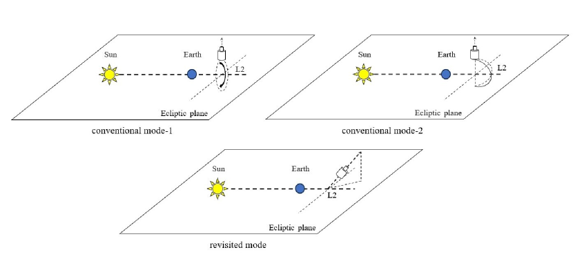
Figure 1: Two types of the observation modes (Ji et al., 2022). Upper panel: conventional mode. Lower panel: revisited mode.

The relative measurement method employed differs fundamentally from the absolute measurement method (Kovalevsky & Seidelmann, 2004), which relies on the precision of a prior catalog. The accuracy of the relative measurement hinges on the precise measurement of angular distances. In absolute measurement, obtaining the positions of reference stars from a prior catalog is imperative, followed by the establishment of a reference frame based on these positions. Subsequently, the positional change information of the target star is ascertained within this reference frame on the local coordinate frame around each target star. Consequently, the accuracy of target star position measurement is limited by the precision of the prior catalog. Even with the most accurate astrometric data available to date, such as Gaia DR3 (Gaia Collaboration et al., 2021), with precision in the order of tens of micro-arcseconds for position, it remains insufficient for detecting stellar disturbance signals caused by Earth-like planets.

The relative measurement method involves measuring the angular distance between the target star and the reference star within the local reference frame spanning the telescope field of view. This change arises from the disparity in proper motion and parallax between the two stars, coupled with the perturbation of the planets affecting the position of the target star. The parameters of relative measurement are illustratively described in Eq. 1,

$$\begin{array}[]{cc}l_{\alpha}(t)=\Delta\alpha_{0}+\Delta\mu_{\alpha}(t-t_{0})+(\pi_{1}F_{\alpha 1}-\pi_{2}F_{\alpha 2})\\ +~{}\alpha_{p}(t)+O(t^{2})\\ l_{\delta}(t)=\Delta\delta_{0}+\Delta\mu_{\delta}(t-t_{0})+(\pi_{1}F_{\delta 1}-\pi_{2}F_{\delta 2})\\ +~{}\delta_{p}(t)+O(t^{2})\end{array}$$ (1)

where $l_{\alpha}$ and $l_{\delta}$ represent two components of the angular distance. $\Delta\alpha_{0}$ and $\Delta\delta_{0}$ denote the initial coordinate difference, while $\Delta\mu_{\alpha}$ and $\Delta\mu_{\delta}$ stand for the proper motion difference. The $F_{\alpha 1},F_{\alpha 2},F_{\delta 1},F_{\delta 1}$ represent the components of the parallax factor of two stars in the directions of right ascension and declination, respectively, and $\alpha_{p}$ and $\delta_{p}$ account for the variations in position due to the planets, while $O(t^{2})$ represents the higher-order terms of the proper motion.

In Eq. 1, there is no necessity to ascertain the actual position coordinates of the reference stars, eliminating the requirements for a prior catalog. Consequently, the measurement accuracy of angular distance has become a crucial factor in determining the ability of exoplanet detection. To achieve such high-precision astrometry, Theia previously imposed strict requirements on the instruments (Malbet et al., 2021) and attempted to calibrate telescope distortions by using the positions of reference stars obtained from the Gaia prior star catalog (Malbet et al., 2022). CHES also considered the low-distortion wide-field telescope optical systems, high-stability attitude control and high-precision thermal control technologies to ensure measurements reach micro-arcsecond accuracy in angular distance (Ji et al., 2022, 2024).

The measurement of angular distance in actual observations involves determining the position and distance between the target star and the reference star on the focal plane. It is crucial to consider the projection relationship from the celestial sphere to the focal plane when addressing angular distance on the celestial sphere and distance on the focal plane. During the observation process, no reference frame is available in the FOV as it does not rely on a priori catalog. Typically, the target star is positioned at the center of the FOV, surrounded by multiple distributed reference stars. Special cases may arise, such as when the target of observation is a binary star, exemplified by * i Boo (van Leeuwen, 2007b), where eleven target stars fall into this category. In such cases, the center of the FOV is directed toward the brighter of the two stars, and the reference stars for both targets within the FOV are identical. Consequently, the two targets can be observed simultaneously, enhancing observation efficiency. An even more uncommon scenario is illustrated by the stars V* AK Lep and * gam Lep (Cutri et al., 2003), which are not binaries but are positioned so closely on the celestial sphere that they can be observed concurrently. Figure  2 displays the relative positions of these two stars on the celestial sphere.

Figure 2: The relative positions of V* AK Lep and * gam Lep on the celestial sphere. While these two stars do not form a binary star system, their close proximity on the celestial sphere allows for simultaneous observation of both targets. The FOV is $0.44^{\circ}\times 0.44^{\circ}$. Panel (a): Image from Aladin Sky Atlas (Bonnarel et al., 2000). Panel (b): Simulated observational images of the target stars (Ji et al., 2023).

In previous study, the direction of the optic axis was a subject of discussion (Tan et al., 2022). This discussion highlighted that the target star may not be precisely at the center of the FOV. However, it was established that as long as the range of the point of change falls within a specific range (68 milli-arcseconds at 1 micro-arcsecond), it satisfies the error requirements.

In the CHES mission, the FOV is $0.44^{\circ}\times 0.44^{\circ}$, and the focal plane is equipped with an array of 9 by 9 scientific CMOS detectors. Each detector comprises $4096\times 4096$ pixels. Utilizing the projection relationship and the pertinent instrument parameters, a nonlinear relationship between the radians value of angular distance and the corresponding pixel value is established. One end of the angular distance is anchored at the center of the FOV:

$$P_{D}=\frac{P_{N}}{\tan R}\tan l,$$ (2)

where $P_{D}$ represents the pixel distance from the center of the image point to the center of the FOV. $P_{N}$ refers to the number of pixels from the center to the edge of the detector, with a value of $9\times 4096/2$ in this case. $R$ represents the angular radius from the center to the edge of the FOV, as $0.44^{\circ}/2$. $l$ denotes the angular distance between the stars on the celestial sphere and the center of the FOV. The relationship between the pixel distance from the center point and the angular distance from the center point on the celestial sphere is not strictly linear but exhibits an approximate linearity.

The angular distance between the target star and the reference star can also be employed for the indirect measurement of changes in angular distance between reference stars, utilizing spherical triangulation. These changes in angular distance among reference stars are also on the order of micro-arcseconds, providing valuable information for scientific inquiries such as identifying the presence of binaries in reference stars.

3 Photon noise and observation time

In observations at the micro-arcsecond scale, the impact of photon noise on observational accuracy becomes non-negligible. The error due to photon noise is inversely proportional to the number of photons received, with lower noise levels for a target star surrounded by a greater number of reference stars in the FOV. Consequently, no more than 12 brightest reference stars, along with the target star, are chosen to compute the number of photons received per unit time. The incorporation of additional reference stars increases the photon count for them, thereby reducing the influence of photon noise.

The error arising from photon noise is directly proportional to the square root of the inverse of the product of the number of observations and the exposure time for each observation, expressed as $\sigma\propto(N_{vis}\times t_{vis})^{-1/2}$ (Malbet et al., 2021). Consequently, increasing both the number of observations and the exposure time for each observation proves effective in reducing photon noise. We hope to discover Earth-like planets around the target star, and therefore need to observe signals of periodic motions of the host star due to the presence of Earth-like planets in the habitable zone of the target star.

We calculate the range of habitable zone of the Earth-like planets based on the effective temperature and luminosity of each target star (Kopparapu et al., 2014):

$$S_{eff}=S_{eff\odot}+aT_{\star}+bT_{\star}^{2}+cT_{\star}^{3}+dT_{\star}^{4},$$ (3)

where $T_{\star}=T_{eff}-5780~{}\rm{K}$ and the coefficients of $T_{\star}$ are parameters related to the planetary mass. In this context, the planetary mass is assumed to be one Earth mass. The corresponding range of habitable zones is given by the following equation (Kopparapu et al., 2014):

$$D_{HZ}=\left(\frac{L/L_{\odot}}{S_{eff}}\right)^{0.5}\ \mathrm{AU},$$ (4)

where $L/L_{\odot}$ is the luminosity of the star compared to the Sun.

We take the centre of the habitable zone as the orbital semi-major axis of the planet and calculate the strength of the signal(Malbet et al., 2012):

$$\alpha=0.3\left(\frac{M_{P}}{M_{\oplus}}\right)\left(\frac{a}{1\rm~{}AU}\right)\left(\frac{M_{\star}}{M_{\odot}}\right)^{-1}\left(\frac{D}{10\rm~{}pc}\right)^{-1}\rm\mu as,$$ (5)

where the $M_{P}$ and $M_{\star}$ are the mass of the planet and the host star, $a$ is the semi-major axis base on the habitable zone and $D$ is the distance of the host star. We take the classical signal-to-noise ratio SNR = 6 (Brown, 2009) to estimate the upper limit of the allowable error due to photonic noise $\sigma=A/\rm SNR$. This will ultimately be used to determine the precision and time needed to observe Earth-like planets.

In the observation design, to ensure precision in the measurements, the CHES satellite will conduct a 2.5-hour calibration after each scientific observation of the target star, comprising 2 hours for optical aberration correction and 0.5 hours for focal plane calibration (Ji et al., 2022). Consequently, for a given observation target, optimizing the observation time for a single measurement and reducing the overall number of observations can minimize the calibration time share in the entire observation cycle, thereby enhancing observation efficiency. It is essential to strike a balance, ensuring an adequate number of observations to obtain a satisfactory set of stellar astrometric measurements.

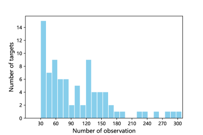
Figure 3: The distribution of the proposed number of observations for each target star is determined by various parameters. The average number of observations was approximately 100. The minimum required number of observations is set at 30, while the maximum number of observations reaches 308.

The ultimate design entails observing each target star a minimum of 30 times during the 5-year observation period, with each scientific observation lasting no less than 0.5 hours. The distribution of the number of observations is presented in Fig 3. The specific number of observations for each target star is detailed in the Appendix.

4 Prioritization of target stars observation

We further filtered out the target stars that require less than about 300 observations based on the number of observations of the target stars in the previous section, totaling 94 target stars. Among them, there are 11 groups of two target stars in the same FOV, which will be observed at the same time, resulting in a total of 83 observation targets. For these targets, an observing strategy will be developed based on that one in the FOV that requires a higher number of observations. Given that the time required for a single observation is no less than 3 hours, prioritization of target stars is essential to efficiently observe scientifically interesting ones within the designated operational timeframe. The prioritization of observations is determined by considering the following five factors:

1. D: Distance. We intend to observe nearly 100 stars within 10 pc, and as a result, we will prioritize observations from the closest to the farthest in terms of distance. The value for distance prioritization ranges from 1.0 for the closest target star (* alf Cen A, 1.3459 pc (Voges et al., 2000)) to 0.8 for the farthest target star (* i Boo A, 12.9450 pc (Gaia Collaboration, 2018)). The other target stars will be assigned values between 0.8 and 1.0 based on their respective distances.

2. M: Magnitude. Considering the impact of photon noise, we analyze the effect of magnitude on observing priority, taking into account the illumination of the target star.

   $$\frac{E_{2}}{E_{1}}=10^{0.4\times\Delta M}$$ (6)

   The calculation of the effect of magnitude on observations is based on the illumination of a target star with a magnitude of 3. For targets with a magnitude less than or equal to 3, this factor is assigned a value of 1. For the target with the minimum magnitude (HD 32450, magnitude 9.6368 (Gaia Collaboration, 2020)), this factor is assigned a value of 0.8. For other targets, the factor is assigned values in the range of 0.8 to 1.0, depending on the illumination.

3. N: Number of the reference stars. The number of reference stars affects both measurement error and the impact of photon noise. Reference stars in the FOV are generally selected with magnitudes not exceeding 13. For some target stars in a dense star field, there may be numerous reference stars. In actual observation, the brightest reference stars are chosen to measure the angular distance between them and the target star. In this prioritization, we consider cases with no more than 12 reference stars. For cases with more than 12, their influence on priority is equated to that of 12 reference stars. The values representing their influence on priority are as follows:

   Value : $>12$:1.0; 8-11 : 0.9 ; 6-7 : 0.8 : $<6$ : 0.7

4. E: Exoplanet. Kepler/K2 and TESS or ground-based telescopes, have detected a large number of exoplanets and candidates using transiting or radial velocity methods. The target stars selected for CHES include those that have been previously confirmed to have exoplanets or are tentative candidates. For instance, tau Cet has four identified planets (Feng et al., 2017b): tau Cet e, tau Cet f, tau Cet g, and tau Cet h. Other target stars with confirmed exoplanets and tentative candidates are listed in Table 1. The planetary systems in Table 1 were all detected using the radial velocity method. Among them, HD 219134 b and HD 219134 c were also detected using the transit method. The CHES will further confirm the tentative candidates but also provide true planetary mass and three-dimensional orbits for the confirmed planets, thereby leading to a full understanding of planetary formation and evolution. The impact of the presence of exoplanets on priority is determined as follows:

   Value : Confirmed planets or tentative candidate: 1.0; Uncomfirmed: 0.8

5. B: Binary or more stars. This factor takes into account the possibility of using the same reference star in the same FOV for simultaneous exoplanet detection of the binary star, thereby improving observation efficiency. Additionally, observations of binary stars can yield high-precision astrometric data. The special case mentioned in Section 2 involving stars V* AK Lep and * gam Lep is also considered here as a binary star assignment to this factor.

   Value : Binary or more stars: 1.0; single stars: 0.8

The priority of each target star is determined by a combination of the five factors mentioned above, represented as ${rankindex=D*M*N*E*B}$. The final priority is obtained by normalizing this value and is presented in the Appendix. A higher value indicates a higher priority for observation. Given the current number of established observations and the exposure time for a single observation, all observation targets can receive sufficient observation time. This prioritization of observation targets serves as a strategy for discarding certain observation targets in scenarios where additional observation tasks are introduced and there is insufficient observation time.

Table 1: Confirmed planets and tentative planets in CHES targets.

Host name	Other name	Confirmed Planet	Tentative Planet
61 Vir	-	61 Vir b (1,2); 61 Vir c (1,2)	61 Vir d (2)
HD 20794	e Eri	HD 20794 b (3,4); HD 20794 c (3,4); HD 20794 d (3,4)	HD 20794 e (4)
tau Cet	-	tau Cet e (5); tau Cet f (5); tau Cet g (5); tau Cet h (5)	tau Cet b (6); tau Cet c (6); tau Cet d (6)
HD 102365	-	HD 102365 b (7)	-
HD 147513	-	HD 147513 b (8)	-
HD 69830	-	HD 69830 b (2,9); HD 69830 c (2,9); HD 69830 d (2,9)	-
eps Eri	-	eps Eri b (2,10,11,12,13)	-
eps Ind	-	eps Ind A b (14,15)	-
HD 26965	omi02 Eri	-	HD 26965 b (16)
HD 131977	-	-	HD 131977 b (17)
HD 219134	-	HD 219134 b (2,18,19,20,21,22); HD 219134 c (2,18,19,21,22); HD 219134 d (2,18,19,22); HD 219134 f (2,18,19,22); HD 219134 h (2,22,23)	HD 219134 g (22)
HD 192310	-	HD 192310 b (2,4,24)	HD 192310 c (4)
GJ 86	HD 13445	GJ 86 b (25,26,27)	-
HD 3651	54 Psc	HD 3651 b (2,27,28,29,30)	-
HD 85512	-	HD 85512 b (4,25)	-
HD 40307	-	HD 40307 b (31,32,33); HD 40307 c (31,32,33); HD 40307 d (31,32,33); HD 40307 f (31,32,33); HD 40307 g (31,32)	-
lam Ser	-	-	lam Ser b (2)
HD 115404	LHS 2713	-	HD 115404 A b (34); HD 115404 A c (34)

Note. — References:(1)Vogt et al. (2010); (2)Rosenthal et al. (2021); (3)Feng et al. (2017a); (4)Pepe et al. (2011); (5)Feng et al. (2017b); (6)Dumusque et al. (2017); (7)Tinney et al. (2011); (8)Mayor et al. (2004); (9)Lovis et al. (2006); (10)Llop-Sayson et al. (2021); (11)Mawet et al. (2019); (12)Benedict et al. (2006); (13)Hatzes et al. (2000); (14)Feng et al. (2019); (15)Feng et al. (2023); (16)Ma et al. (2018); (17)Gaia Collaboration (2020); (18)Gillon et al. (2017); (19)Motalebi et al. (2015); (20)Kokori et al. (2023); (21)Seager et al. (2021); (22)Vogt et al. (2015); (23)Johnson et al. (2016); (24)Howard et al. (2011); (25)Stassun et al. (2017); (26)Butler et al. (2001); (27)Butler et al. (2006); (28)Wittenmyer et al. (2019); (29)Wittenmyer et al. (2007); (30)Wittenmyer et al. (2009); (31)Tuomi et al. (2013); (32)Brasser et al. (2014); (33)Díaz et al. (2016); (34)Feng et al. (2022)

5 Strategy for observation

Sky survey telescopes typically follow an established scanning law to observe targets entering their FOV (Gaia Collaboration et al., 2016). Given that the observation will encompass the entire celestial sphere, the allocated observation time and the number of observations for each target are limited. Furthermore, adhering to the principles of the scanning law, the time intervals between consecutive observations are relatively extended. This temporal arrangement may result in the oversight of certain periodic signals. Specifically, signals associated with the gravitational effects of exoplanets on the target star may be absent from the observations.

In contrast, CHES focuses on pre-screened candidate targets. Its observation accuracy is higher, and the duration of a single observation is longer. Therefore, we have tailored an observation strategy specifically for CHES. This strategy aims to ensure that the number of observations for each target star is sufficient, while maintaining a uniform time interval between observations. This approach guarantees that the observations capture accurate information about position changes, allowing for the deduction of information about surrounding planets, as well as the masses and orbits of habitable planets.

As detailed in Section  2, the CHES satellite conducts observations in two modes: conventional mode and revisited mode. The two types of conventional modes are interspersed over the five-year observation period and constitute the majority of the observing time. The first type is utilized during the first, third, and fifth years of observations, while the second type is employed for the remaining two years. In both types of conventional modes, the range of observations is fixed relative to the position of the Sun. Consequently, as the satellite trails the Earth in its orbit around L2, each region will be observed twice during a year of observation.

Figure 4 illustrates the regions to be observed at each time during every year. The figure provides a top view of the ecliptic plane, with the Sun’s ecliptic determining the range of ecliptic longitudes observable by satellites. To avoid direct sunlight, the detector observation direction should be at least $60^{\circ}$ away from the direction of the sun, denoted as regions 9-12 in the figure. In the first type of conventional mode, the telescope rotates along the great circle passing through the north and south ecliptic poles, with the observation regions represented in red, green, and purple. In the second type of conventional mode, the telescope observes along two semicircles perpendicular to the ecliptic plane, connected at the north and south poles of the ecliptic, forming an angle of 60 degrees between them. The observation regions are depicted in blue and yellow.

For the annual parallax of a target star, the maximum parallax occurs when the difference between its ecliptic longitude and that of the Sun in the station-centered ecliptic coordinate system is $90^{\circ}$. In the first year, the red region in Fig 4 is selected and overlapped with the purple and green regions, aiming to achieve more observations at the maximum parallax, thereby enhancing the accuracy of the parallax measurement.

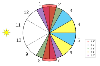
Figure 4: Observed ranges under different years at each moment. In the 1st, 3rd, and 5th years, conventional mode type one will be used. In the 2nd, 4th years, conventional mode type two will be used. To avoid the effects of sunlight, no observations will be conducted in regions 9-12.

In the course of the observation, the satellite is designed to operate with an observing range of 30 degrees in ecliptic longitude. As an example of the regions of observations in the first year, when the ecliptic longitude of the Sun in the station-centered ecliptic coordinate system is $0^{\circ}$, the range of observation can be $75^{\circ}-105^{\circ}$ and $255^{\circ}-285^{\circ}$ in the first year. The satellite is in the vicinity of the L2 point, and the plane of observation is perpendicular to the ecliptic plane, so stars with close ecliptic longitudes in ecliptic coordinates will be observed in close proximity. Figure 5 shows the distribution of targets in ecliptic coordinates.

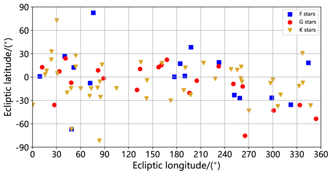
Figure 5: Distribution of targets in ecliptic coordinates. The distribution is not homogeneous, leading to the need to use the re-observation mode to make adjustments in the observation time.

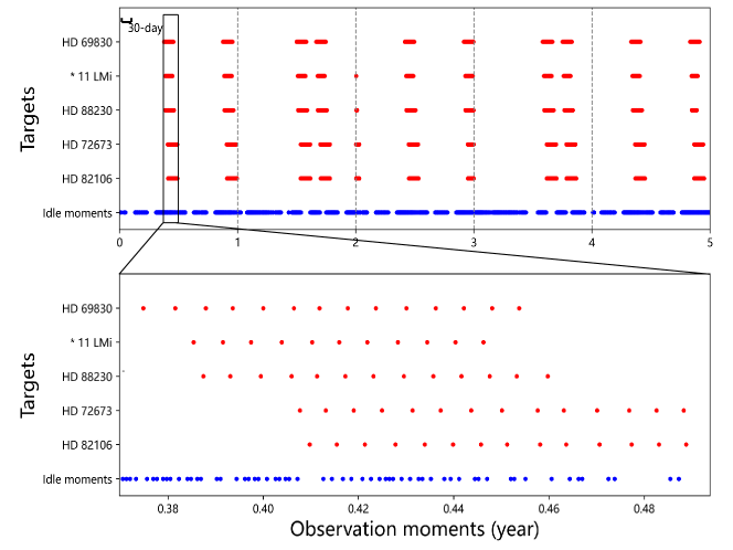
Figure 6: Distribution of observation moments for targets and idle. The five target stars are distributed around 135 degrees of ecliptic longitude. The figure below is a partial enlargement of the black box in the above figure. The order of observation is determined by the position of the target star and the number of observations. At this ecliptic longitude, the distribution of target stars is also relatively sparse, providing idle time in between observations. This idle time can be used to intersperse with other observing tasks.

The satellite moves with the rotation of the Earth at the L2 point, and the range of its observation will also change with time. This allows the regions of observation to cover the entire celestial sphere within the first six months. Since the observations are within a certain range, any target star can be observed for at least two time periods per year, totaling about two months. Within each time period, to ensure that the observation time is as uniform as possible, each observation for a single target star is separated by a certain amount of time. We adopt the following scheme to determine the observation interval for each target star:

$$N_{per}=\frac{\lambda_{width}}{v_{rot}}N_{t},$$ (7)

$$N_{int}=\frac{N_{per}}{N_{obs}/10},$$ (8)

where ${\lambda_{width}}$ represents the observing range of the telescope in ecliptic longitude, set to $30^{\circ}$ in this paper. $v_{rot}$ stands for the speed of the telescope as it rotates along the ecliptic with the Earth at point L2. $N_{t}$ denotes the average number of observations per day. $N_{per}$, $N_{obs}$, and $N_{int}$ represent the total number of observations in the observing range, the total number of observations per star, and the number of intervals between observations, respectively. In a 5-year observation period, each star has 10 subperiods, so the number of observations required in each subperiod is $N_{obs}/10$.

Ultimately, the number and duration of observations of each target star are distributed as uniformly as possible over the 10 observation periods within the 5-year operating time. Meanwhile, to ensure the efficiency of the observation, the positions of the target stars on the celestial sphere during two adjacent observations need to be as close as possible, so as to avoid the detector’s pointing to make reciprocal rotations over a large area.

In addition to the conventional mode, there is the previously mentioned revisited mode. The situations that require the use of the revisited mode are twofold.

1. According to the Section 3, when some target stars require a large number of observations, a sufficient number of observations cannot be accomplished within the time period in which they can be observed, while ensuring that each observation is separated by a certain period of time.

2. As shown in Fig 5, the distribution of target stars at some ecliptic longitudes (e.g., $45^{\circ}$ and $255^{\circ}$) is relatively dense. In this case, although the number of observations required for each of these target stars may be small, the total number of observations required for the target stars within this range is too large. Since the detector has limited time to cover this range, the number of observations is limited, which may result in some target stars not being fully observed for a sufficient number of times during the corresponding observing period.

In both cases, the revisited mode is employed to conduct additional observations during idle moments of the telescope. As mentioned earlier, there are ecliptic longitudes where the distribution of target stars is dense, and conversely, there are some ecliptic longitudes where the distribution of target stars is sparser (e.g., $115^{\circ}$). When observing these target stars, there are telescope idle moments since each star has its own observation interval. Multiple observations of the same target star with a long orbital period in a short period are meaningless. During this idle moments, the telescope can be used for checking and filling in the gaps of the target stars observation due to above two points, but also for other scientific programs.

Based on the single observation time plan described in Section 3 and the observation program described in this section, we formulate the final observation strategy for the target stars. Examples of some target stars with close ecliptic longitudes are shown in Fig 6. The idle moments of the telescope are shown at the bottom of Fig 6. In this observation strategy, the total duration of the satellite’s 5-year operating time is 29,220 hours ($16~{}h\times 365.25\times 5$), with approximately 25,120 hours dedicated to the total observation time on the target stars (about 86 percent of the entire time), as shown in Table 2. The duration available for other observation missions is about 4,100 hours. These times can be distributed at any point during the 5-year operating time by further adjustments to the observing strategy to ensure that the basic observation task is satisfactorily completed, along with other observing tasks.

6 Impact of observing strategies on scientific missions

For the observation strategy, the CHES observation time series is not uniform. The observation moments for targets vary from year to year, and the distribution of observation times shows segmentation. For targets that require more observations, the observations are more discrete. Nevertheless, in the 5-year observation, the observations of each year are complementary to each other, satisfying the needs of scientific observations.

As to the observation design, the target star is positioned at the center of the FOV, ensuring that the results of multiple observations reveal relative changes in the position of the reference star. The celestial motion of the star is a cumulative effect of various motions, and alterations are manifested in the relative proper motion and relative parallax between the target star and the reference star, along with the influence of other factors on the star’s position.

6.1 Proper motion and parallax

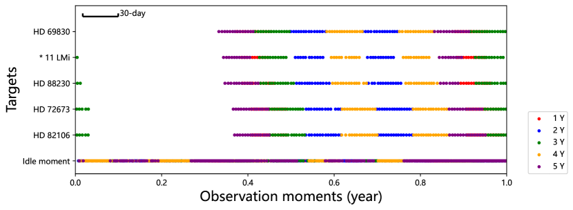
Figure 7: Distribution of observation moments for each target (five for illustration) overlapped in one year.

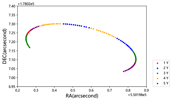
Figure 8: Observable part of the parallax ellipse (Target: HD 88230 (Gaia Collaboration, 2020))

We analyzed the distribution of observation strategies in Fig 6 by consolidating the overlap of observations for each year into a single year, and the results are illustrated in Fig 7. Various colors in the figure denote observations in different years. Maintaining an angle of at least 60 degrees between the observation direction and the Sun is essential to avoid the Sun’s influence. Consequently, for any target star, there must be a one-third of the year during which it cannot be observed, represented by the blank time period in Fig 7.

While the blank time period implies that only two-thirds of the parallax ellipse of the target star will be observed, it is sufficient to fit the parallax with a high degree of precision. According to the observing strategy outlined in the previous section, the observable parallax ellipse can be entirely captured during a 5-year period, with additional observations concentrated when the target star is positioned near its parallax maximum (i.e., the region where the first, third, and fifth years of observations overlap). The observed part is depicted in Fig 8. The proper motion has been eliminated, retaining only the parallax of the target star.

6.2 Coverage of planetary orbit period

The mission’s primary objective is to acquire data on the orbits of planets exhibiting periodic motion around their stars. Consequently, the mission’s efficacy in detecting these orbits will be crucial. The capability to observe the periodic motion of the planets will directly impact the precision of orbit fitting. In the observing strategy outlined in the previous section, observations of any star are not continuous. Thus, it is essential to verify the mission’s capacity to cover the orbital period of the planets in our observations.

We divided the orbital period into 20 parts, each representing 0.05 of the period. A period is considered observed if the observation time for the target star falls within a specific part. Using the observation moments for each target star from the aforementioned observing strategy, we simulated all target stars for planets with varying periods (ranging from 0.1 to 5 years). The distribution of the final coverage is illustrated in Fig 9, with the blue line representing the average value. The coverage of planetary orbital periods consistently exceeds 50 percent and shows an increase with the number of observations, although the changes are not substantial. Our primary focus is on detecting Earth-like planets, i.e., those with periods around 1 year. The coverage of their periods ranges from approximately 60 to 75 percent.

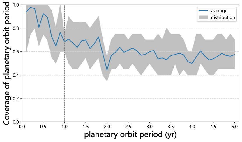
Figure 9: Coverage of planetary orbit period. The blue line indicates the mean value, while the grey ranges indicate the distribution of period coverage under each planetary period for all target stars.

6.3 Simulation solution of planetary parameters

Figure 10: The black dotted line represent the simulated periodic motion of the target star caused by the presence of planet around it. The grey forks in (a) and dots with error bars in (b) depict the residual motion that remains after eliminating the relative proper motion and parallax of the target and reference stars in the fit based on the relative measurement method. The red dots illustrate the outcome of the fit to this periodic motion. Left panel: Component at right ascension and declination. Right panel: Periodic motion of the target star on the celestial sphere.

Figure 11: The black dotted line represent the simulated periodic motion of the target star caused by the presence of both planets around it. The grey forks in (a) and dots with error bars in (b) depict the residual motion that remains after eliminating the relative proper motion and parallax of the target and reference stars in the fit with the relative measurement method. Left panel: Component at right ascension and declination. Right panel: Periodic motion of the target star on the celestial sphere.

Figure 12: The black dotted line in the upper and lower panels represent the simulated periodic motion of the target star caused by the presence of two planets around it, respectively. (a) and (b) correspond to the inner Earth-like planets. (c) and (d) correspond to the outer planet. The red dots illustrate the outcome of the fit to these periodic motion. Left panel: Component at right ascension and declination. Right panel: Periodic motion of the target star on the celestial sphere.

We chose HD 88230 (Gaia Collaboration, 2020) as an illustrative example and conducted two simulations incorporating relevant parameters. The first example considers the scenario of an Earth-like planet at 1 AU from the star, while the second run is related to an additional planet with a mass 20 times that of Earth located at 2 AU. During these simulations, the target star undergoes periodic motion induced by the gravitational influence of the planets, resulting in positional variations at the micro-arcsecond level. Following the observing strategy outlined in this work, we simulated the FOV of the target star as observed by the detector from the L2 point at various time points. This field of view encompasses positional information of both the target and reference stars. Subsequently, we employed a fitting procedure on the angular distance data, incorporating a Gaussian error based on the detection capability.

As outlined in the preceding section, this mission relies on the principle of relative measurement to capture the periodic motion of the target star. Consequently, during the observation and data processing of the target star and the reference star, it is unnecessary to acquire precise position information of the target star. Simultaneously, obtaining position information for the target star with the required high accuracy (on the order of micro-arcseconds) is not feasible.

Based on the fitting method of relative measurements (Bao et al., 2024b), we fit the relative proper motions, and the parallaxes. The residual represents the periodic motion of the target star due to the presence of the planet. The orbital fit to this residual yields the orbital parameters. Figure 10 shows the results of the orbital fitting in the right ascension and declination directions, along with the simulated periodic motion of the star based on the observed moments from the observing strategy. Figure 11 and 12 illustrate the presence of two planets orbiting the star. Table 3 summarizes the fitting parameters for one-planet and two-planet systems, respectively, along with the initial parameters, indicating that the fitted values are in close to the given data.

Table 2: Time allocation in CHES mission.

Program	Observation mode	Used time (h)	Mission fraction
CHES targets	Conventional mode	21451	0.734
	Revisited mode	3669	0.126
	Total	25120	0.860
Open time		4100	0.140
Overall		29220	1.00

7 Conclusions and Discussions

In this work, we conduct an extensive study of the optimization of observation strategy for the target stars in the CHES mission. The primary objective of CHES is to identify and characterize potentially habitable Earth-like planets or super-Earths orbiting approximately 100 solar-type stars within a distance of 10 parsecs from our solar system. CHES accomplishes high-precision astrometric measurements by tracking angular distance variations between the target star and reference stars. A thorough analysis of relevant parameters for both target and reference stars has been carried out to determine required observation accuracy, the number of observations required, and priority assignment for each target star.

Here two observation modes of the observing strategy involve adopting different observation areas in different years, and measures such as peaks and troughs are adjusted to ensure a sufficient number of observations of all target stars within a 5-year period. With this observing strategy, every target star will be observed at least once within a six-month period. Over the course of the 5-year period, a total of 29,220 hours are available for scientific observations, with 25,120 hours (86 percent) designated for observing target stars, and the remaining 4,100 hours allocated to other programs. Each target star is assigned no fewer than 30 observations, with a maximum of 308 observations and an average of approximately 100 observations. Reflecting the motion of a star by the variation of the angular distance between the reference star and the target star, CHES is not limited to the detection of terrestrial planets but can also detect factors affecting the reflex motion of the star, such as the motion of a binary star and its evolution, and the detection of black holes. The design of the observing strategy allows for the flexible allocation of time for other observing tasks, ensuring that CHES can achieve its utmost scientific goals while completing additional observation tasks.

There is scope for optimization within this observation strategy. During observations, to mitigate the impact of direct sunlight on the detector, the target star is discontinued from observation when the angle between the sun and the target star falls below a certain threshold. In the formulation of this strategy, this threshold angle is set to 60 degrees. Consequently, the target star remains unobserved for one third of the year, as shown in Figure 8. This angle is determined by the telescope’s design, and optimizing it could result in more comprehensive time-series observations.

Table 3: The fitting of planetary orbital parameters with simulated relative measurements.

Object	Parameters	Single planet fitting	Double planet fitting	Given values
Inner planet	$\cos i$	$0.853^{+0.013}_{-0.496}$	$0.803^{+0.135}_{-0.138}$	0.867
	$e\cos\omega$	$0.042^{+0.434}_{-0.003}$	$0.031^{+0.125}_{-0.161}$	0.087
	$e\sin\omega$	$0.000^{+0.662}_{-0.000}$	$0.095^{+0.729}_{-0.084}$	0.0500
	$\Omega$ (rad)	$3.14^{+0.01}_{-2.31}$	$1.52^{+1.08}_{-1.01}$	1.05
	$M_{0}$ (rad)	$2.69^{+0.32}_{-0.16}$	$1.54^{+1.06}_{-1.03}$	0.79
	Mass ($M_{\oplus}$)	$0.969^{+0.733}_{-0.016}$	$0.958^{+0.035}_{-0.033}$	1.000
	Period (days)	$466.14^{+0.38}_{-102.30}$	$453.89^{+17.63}_{-16.62}$	447.67
Outer planet	$\cos i$		$0.730^{+0.047}_{-0.022}$	0.867
	$e\cos\omega$		$0.070^{+0.017}_{-0.014}$	0.00
	$e\sin\omega$		$0.171^{+0.013}_{-0.027}$	0.100
	$\Omega$ (rad)		$0.763^{+0.103}_{-0.049}$	0.785
	$M_{0}$ (rad)		$0.383^{+0.056}_{-0.026}$	1.047
	Mass ($M_{\oplus}$)		$19.402^{+0.596}_{-0.299}$	20.000
	Period (days)		$1229.51^{+37.42}_{-21.82}$	1266.21

Note. — $i$ : inclination; $\omega$ : argument of periapsis; $e$ : eccentricity; $\Omega$ : longitude of ascending node ;$M$ : mean anomaly; $M_{\oplus}$ : mass of the earth

The targets are identified within this observing strategy, which also requires that observations alternate between these target stars. Consequently, this leads to a non-uniform distribution of observation times for the targets, further compounded by the fact that the observing strategy changes from year to year. While this variability enables CHES to encompass, to the greatest extent, the parallax period of the target stars and the period of planetary perturbations over the overall 5-year observation period, the resulting non-uniform sampling also impacts the fitting process. In the future study, additional techniques or algorithms are required to minimize errors and ensure micro-arcsecond precision measurements and planetary orbit detection.

Appendix A Parameters related to the observed target

In Section 4, we investigate the prioritization of observing targets, and the outcomes are elucidated in Table LABEL:table:appendix. Ultimately, we carefully selected 94 target stars based on the criterion of the number of observations, with exclusion of those demanding an excessive number (more than 300). For the case where there are two target stars in the field of view (11 groups in total), they will be observed simultaneously, so the target star requiring more observations dominates in the prioritization calculation. The data columns in the table present five factors affecting priority: distance, V-band magnitude, number of reference stars, confirmed to have exoplanet or tentative candidates, and whether the star is part of a binary system. In the ”Binary” column, the case of three stars is also included. We also present the spectral type of the target star in one of the columns. In the last two columns, we provide the number of observations and their priority.

Table 4: Priority of target stars and number of observations

Target stars	Distance	Magnitude	Nref	Exoplanet	Binary	Spectral Type	Nobs	Priority
	(pc)	V		confirm				%
alf Cen A	1.35	0.01	59	N	Y	G2V	30	100.0
(alf Cen B)
omi02 Eri	5.04	4.43	16	Y	Y	K0V	30	99.89
alf CMi	3.51	0.37	31	N	Y	F5IV	30	96.26
eps Eri	3.20	3.73	16	Y	N	K2V	30	87.31
eta Cas A	5.84	3.44	38	N	Y	F9V	30	86.10
(eta Cas B)
chi Dra	8.30	3.58	25	N	Y	F7V	57	80.72
61 Cyg B	3.49	6.03	46	N	Y	K7V	78	78.20
(61 Cyg A)
36 Oph B	5.96	5.03	20	N	Y	K1V	71	76.45
(36 Oph A)
70 Oph B	5.12	6.07	33	N	Y	K4V	30	75.88
HD 191408	6.02	5.32	18	N	Y	K2.5V	30	75.71
HD 131977	5.88	5.72	14	N	N	K4V	114	75.23
HD 219134	6.53	5.57	32	Y	N	K3V	30	74.53
bet Hyi	5.84	2.79	20	N	N	G0V	31	73.80
HD 156384	6.84	5.89	13	N	Y	K3V+K5V	42	73.67
61 Vir	8.51	4.74	12	Y	N	G7V	61	73.64
ksi Boo B	6.75	6.82	13	N	Y	K5Ve	52	73.07
(ksi Boo A)
eps Ind	3.64	4.69	10	Y	N	K5V	31	72.78
HD 102365	9.29	4.88	16	Y	N	G2V	60	72.08
p Eri B	8.19	5.80	17	N	Y	K2V	119	71.88
(p Eri A)
gam Vir B	12.7	3.85	13	N	Y	F0mF2V	138	71.63
(gam Vir A)
41 Ara A	8.79	5.52	36	N	Y	G9V	83	71.43
tau Cet	3.60	3.50	7	Y	N	G8V	30	71.20
HD 192310	8.80	5.72	12	Y	N	K2+V	107	71.12
iot Peg	11.8	4.20	27	N	Y	F5V	51	71.00
V* AK Lep	8.90	6.15	21	N	Y	K3	119	70.52
(gam Lep)
HD 32450	8.38	8.32	14	N	Y	K7V	62	70.41
pi.03 Ori	8.04	3.19	19	N	N	F6V	30	68.49
lam Ser	11.8	5.03	24	Y	N	G0-V	119	68.06
zet TrA	12.2	5.46	29	N	Y	F9V	102	66.73
HD 85512	11.3	8.83	32	Y	N	K6Vk	92	66.35
zet01 Ret	12.0	6.18	12	N	Y	G2.5	155	66.10
(zet02 Ret)
HD 38A	11.5	10.2	21	N	Y	K6V	126	65.98
85 Peg	12.7	6.42	15	N	Y	G5V	130	65.08
HD 69830	12.6	6.74	24	Y	N	G8:V	160	65.02
HD 40307	12.9	8.10	23	Y	N	K2.5V	121	64.13
e Eri	6.00	4.27	6	Y	N	G6V	49	63.42
bet TrA	12.4	3.14	53	N	N	F1V	121	63.21
sig Dra	5.77	4.68	27	N	N	K0V	39	62.25
HD 88230	4.87	6.61	16	N	N	K6V	125	60.64
zet Tuc	8.53	4.23	15	N	N	F9.5V	51	60.57
gam Pav	9.27	4.22	20	N	N	F9V	60	59.73
V* V2215 Oph	5.95	6.34	21	N	N	K5V	57	59.58
chi01 Ori	8.84	4.40	29	N	N	G0V	60	59.56
mu. Cas	7.55	5.17	22	N	N	G5Vb	33	59.07
107 Psc	7.61	5.24	12	N	N	K1V	65	58.89
LHS 2713	11.0	6.66	3	Y	Y	K2V	220	58.85
i Boo A	12.9	5.72	10	N	Y	F5V	139	58.76
(i Boo B)
HD 147513	12.9	6.02	9	Y	N	G5V	153	58.52
V* TW PsA	7.61	6.48	15	N	N	K4Ve	101	57.65
HD 157881	7.71	7.56	13	N	N	K7V	39	57.17
gam Ser	11.3	4.34	17	N	N	F6IV	59	56.92
61 UMa	9.58	5.34	12	N	N	G8V	88	56.49
HD 32147	8.85	6.21	20	N	N	K3+V	175	56.43
HD 50281	8.75	6.57	42	N	N	K3.5V	50	56.34
tet Per	11.1	4.62	23	N	N	F8V	67	56.19
alf Men	10.2	5.09	25	N	N	G7V	81	56.18
HD 100623	9.54	5.98	21	N	N	K0V	143	55.82
HD 10780	10.0	5.63	21	N	N	K0V	97	55.59
HD 17925	10.4	6.05	12	N	N	V-K1V	145	54.85
zet Dor	11.6	5.22	30	N	N	F9VFe-0.5	85	54.35
HD 13445	10.8	6.17	6	Y	N	K1.5V	231	54.29
HD 154363	10.5	7.71	18	N	N	K4/5V	259	54.10
11 LMi	11.2	6.11	12	N	N	G8V	109	53.86
bet Com	9.18	4.25	8	N	N	F9.5V	70	53.74
54 Psc	11.1	6.71	19	Y	N	K0.5V	168	53.62
lam Aur	12.5	5.33	27	N	N	G1.5IV	70	53.21
V* V2689 Ori	11.4	10.3	27	N	N	K6V	166	52.87
CD-57 1079	11.7	10.4	28	N	N	K7Vk	140	52.58
HD 4628	7.4	5.74	9	N	N	K2.5V	80	52.57
HD 72673	12.2	7.17	32	N	N	K1V	288	52.31
HD 37394	12.3	7.07	18	N	N	K1	163	52.22
kap01 Cet	9.15	4.85	11	N	N	G5V	74	52.11
HD 21531	12.5	9.71	7	N	Y	K5V	143	51.71
HD 82106	12.8	8.22	18	N	N	K3V	308	51.47
HD 101581	12.8	8.83	12	N	N	K4.5Vk	132	51.42
ksi UMa B	8.73	4.73	5	N	Y	G2V	82	51.34
(ksi UMa A)
HD 36003	12.9	8.78	25	N	N	K5V	150	51.26
HD 217357	8.23	7.87	8	N	N	K7+Vk	187	50.89
HD 103095	9.18	6.45	9	N	N	K1V	277	50.33
12 Oph	9.92	5.77	11	N	N	K0V	124	50.03
bet Vir	11.1	3.60	7	N	N	F9V	47	48.69
bet CVn	8.61	4.25	7	N	N	G0V	60	48.32
HD 222237	11.5	8.09	11	N	N	K3+V	101	47.66

References

- Anglada-Escudé et al. (2016) Anglada-Escudé, G., Amado, P. J., Barnes, J., et al. 2016, Nature, 536, 437, doi: 10.1038/nature19106
- Baba & Kawata (2020) Baba, J., & Kawata, D. 2020, MNRAS, 492, 4500, doi: 10.1093/mnras/staa140
- Bao et al. (2024a) Bao, C., Ji, J., Tan, D., et al. 2024a, AJ, 167, 286, doi: 10.3847/1538-3881/ad4031
- Bao et al. (2024b) —. 2024b, Acta Astronomica Sinica, 65, 39
- Batalha et al. (2013) Batalha, N. M., Rowe, J. F., Bryson, S. T., et al. 2013, ApJS, 204, 24, doi: 10.1088/0067-0049/204/2/24
- Benedict et al. (2006) Benedict, G. F., McArthur, B. E., Gatewood, G., et al. 2006, AJ, 132, 2206, doi: 10.1086/508323
- Bonnarel et al. (2000) Bonnarel, F., Fernique, P., Bienaymé, O., et al. 2000, A&AS, 143, 33, doi: 10.1051/aas:2000331
- Borucki et al. (2010) Borucki, W. J., Koch, D., Basri, G., et al. 2010, Science, 327, 977, doi: 10.1126/science.1185402
- Borucki et al. (2011) Borucki, W. J., Koch, D. G., Basri, G., et al. 2011, ApJ, 736, 19, doi: 10.1088/0004-637X/736/1/19
- Brasser et al. (2014) Brasser, R., Ida, S., & Kokubo, E. 2014, MNRAS, 440, 3685, doi: 10.1093/mnras/stu555
- Brown (2009) Brown, R. A. 2009, ApJ, 699, 711, doi: 10.1088/0004-637X/699/1/711
- Butler et al. (2001) Butler, R. P., Tinney, C. G., Marcy, G. W., et al. 2001, ApJ, 555, 410, doi: 10.1086/321467
- Butler et al. (2004) Butler, R. P., Vogt, S. S., Marcy, G. W., et al. 2004, ApJ, 617, 580, doi: 10.1086/425173
- Butler et al. (2006) Butler, R. P., Wright, J. T., Marcy, G. W., et al. 2006, ApJ, 646, 505, doi: 10.1086/504701
- Casertano et al. (2008) Casertano, S., Lattanzi, M. G., Sozzetti, A., et al. 2008, A&A, 482, 699, doi: 10.1051/0004-6361:20078997
- Catanzarite et al. (2006) Catanzarite, J., Shao, M., Tanner, A., Unwin, S., & Yu, J. 2006, PASP, 118, 1319, doi: 10.1086/504442
- Charbonneau et al. (2000) Charbonneau, D., Brown, T. M., Latham, D. W., & Mayor, M. 2000, ApJ, 529, L45, doi: 10.1086/312457
- Chauvin et al. (2004) Chauvin, G., Lagrange, A. M., Dumas, C., et al. 2004, A&A, 425, L29, doi: 10.1051/0004-6361:200400056
- Crossfield (2013) Crossfield, I. J. M. 2013, A&A, 551, A99, doi: 10.1051/0004-6361/201220914
- Curiel et al. (2022) Curiel, S., Ortiz-León, G. N., Mioduszewski, A. J., & Sanchez-Bermudez, J. 2022, AJ, 164, 93, doi: 10.3847/1538-3881/ac7c66
- Cutri et al. (2003) Cutri, R. M., Skrutskie, M. F., van Dyk, S., et al. 2003, VizieR Online Data Catalog, II/246
- Díaz et al. (2016) Díaz, R. F., Ségransan, D., Udry, S., et al. 2016, A&A, 585, A134, doi: 10.1051/0004-6361/201526729
- Dumusque et al. (2017) Dumusque, X., Borsa, F., Damasso, M., et al. 2017, A&A, 598, A133, doi: 10.1051/0004-6361/201628671
- Feng et al. (2019) Feng, F., Anglada-Escudé, G., Tuomi, M., et al. 2019, MNRAS, 490, 5002, doi: 10.1093/mnras/stz2912
- Feng et al. (2023) Feng, F., Butler, R. P., Vogt, S. S., Holden, B., & Rui, Y. 2023, MNRAS, 525, 607, doi: 10.1093/mnras/stad2297
- Feng et al. (2017a) Feng, F., Tuomi, M., & Jones, H. R. A. 2017a, A&A, 605, A103, doi: 10.1051/0004-6361/201730406
- Feng et al. (2017b) Feng, F., Tuomi, M., Jones, H. R. A., et al. 2017b, AJ, 154, 135, doi: 10.3847/1538-3881/aa83b4
- Feng et al. (2022) Feng, F., Butler, R. P., Vogt, S. S., et al. 2022, ApJS, 262, 21, doi: 10.3847/1538-4365/ac7e57
- Gaia Collaboration (2018) Gaia Collaboration. 2018, VizieR Online Data Catalog, I/345, doi: 10.26093/cds/vizier.1345
- Gaia Collaboration (2020) —. 2020, VizieR Online Data Catalog, I/350, doi: 10.26093/cds/vizier.1350
- Gaia Collaboration et al. (2016) Gaia Collaboration, Prusti, T., de Bruijne, J. H. J., et al. 2016, A&A, 595, A1, doi: 10.1051/0004-6361/201629272
- Gaia Collaboration et al. (2021) Gaia Collaboration, Brown, A. G. A., Vallenari, A., et al. 2021, A&A, 649, A1, doi: 10.1051/0004-6361/202039657
- Gaudi et al. (2020) Gaudi, B. S., Seager, S., Mennesson, B., et al. 2020, arXiv e-prints, arXiv:2001.06683, doi: 10.48550/arXiv.2001.06683
- Gillon et al. (2017) Gillon, M., Triaud, A. H. M. J., Demory, B.-O., et al. 2017, Nature, 542, 456, doi: 10.1038/nature21360
- Gilmozzi & Spyromilio (2007) Gilmozzi, R., & Spyromilio, J. 2007, The Messenger, 127, 11
- Hatzes et al. (2000) Hatzes, A. P., Cochran, W. D., McArthur, B., et al. 2000, ApJ, 544, L145, doi: 10.1086/317319
- Howard et al. (2011) Howard, A. W., Johnson, J. A., Marcy, G. W., et al. 2011, ApJ, 730, 10, doi: 10.1088/0004-637X/730/1/10
- Howell et al. (2014) Howell, S. B., Sobeck, C., Haas, M., et al. 2014, PASP, 126, 398, doi: 10.1086/676406
- Ji et al. (2023) Ji, J., Tan, D., Bao, C., et al. 2023, Research in Astronomy and Astrophysics, 23, 125015, doi: 10.1088/1674-4527/ad0499
- Ji & Wang (2020) Ji, J., & Wang, S. 2020, Chinese Journal of Space Science, 40, 729, doi: 10.11728/cjss2020.05.729
- Ji et al. (2024) Ji, J., Li, H., Zhang, J., et al. 2024, Chinese Journal of Space Science, 44, 193, doi: 10.11728/cjss2024.02.yg03
- Ji et al. (2022) Ji, J.-H., Li, H.-T., Zhang, J.-B., et al. 2022, Research in Astronomy and Astrophysics, 22, 072003, doi: 10.1088/1674-4527/ac77e4
- Johns et al. (2012) Johns, M., McCarthy, P., Raybould, K., et al. 2012, in Society of Photo-Optical Instrumentation Engineers (SPIE) Conference Series, Vol. 8444, Ground-based and Airborne Telescopes IV, ed. L. M. Stepp, R. Gilmozzi, & H. J. Hall, 84441H, doi: 10.1117/12.926716
- Johnson et al. (2016) Johnson, M. C., Endl, M., Cochran, W. D., et al. 2016, ApJ, 821, 74, doi: 10.3847/0004-637X/821/2/74
- Kawata et al. (2023) Kawata, D., Kawahara, H., Gouda, N., et al. 2023, arXiv e-prints, arXiv:2307.05666, doi: 10.48550/arXiv.2307.05666
- Kokori et al. (2023) Kokori, A., Tsiaras, A., Edwards, B., et al. 2023, ApJS, 265, 4, doi: 10.3847/1538-4365/ac9da4
- Kopparapu et al. (2014) Kopparapu, R. K., Ramirez, R. M., SchottelKotte, J., et al. 2014, ApJ, 787, L29, doi: 10.1088/2041-8205/787/2/L29
- Kovalevsky & Seidelmann (2004) Kovalevsky, J., & Seidelmann, P. K. 2004, Fundamentals of Astrometry
- Lattanzi et al. (2000) Lattanzi, M. G., Spagna, A., Sozzetti, A., & Casertano, S. 2000, MNRAS, 317, 211, doi: 10.1046/j.1365-8711.2000.03637.x
- Lindegren et al. (2021) Lindegren, L., Klioner, S. A., Hernández, J., et al. 2021, A&A, 649, A2, doi: 10.1051/0004-6361/202039709
- Llop-Sayson et al. (2021) Llop-Sayson, J., Wang, J. J., Ruffio, J.-B., et al. 2021, AJ, 162, 181, doi: 10.3847/1538-3881/ac134a
- Lovis et al. (2006) Lovis, C., Mayor, M., Pepe, F., et al. 2006, Nature, 441, 305, doi: 10.1038/nature04828
- Lustig-Yaeger et al. (2019) Lustig-Yaeger, J., Meadows, V. S., & Lincowski, A. P. 2019, AJ, 158, 27, doi: 10.3847/1538-3881/ab21e0
- Ma et al. (2018) Ma, B., Ge, J., Muterspaugh, M., et al. 2018, MNRAS, 480, 2411, doi: 10.1093/mnras/sty1933
- Malbet et al. (2012) Malbet, F., Léger, A., Shao, M., et al. 2012, Experimental Astronomy, 34, 385, doi: 10.1007/s10686-011-9246-1
- Malbet et al. (2021) Malbet, F., Boehm, C., Krone-Martins, A., et al. 2021, Experimental Astronomy, 51, 845–886, doi: 10.1007/s10686-021-09781-1
- Malbet et al. (2022) Malbet, F., Labadie, L., Sozzetti, A., et al. 2022, in Society of Photo-Optical Instrumentation Engineers (SPIE) Conference Series, Vol. 12180, Space Telescopes and Instrumentation 2022: Optical, Infrared, and Millimeter Wave, ed. L. E. Coyle, S. Matsuura, & M. D. Perrin, 121801F, doi: 10.1117/12.2629927
- Mamajek & Stapelfeldt (2024) Mamajek, E., & Stapelfeldt, K. 2024, arXiv e-prints, arXiv:2402.12414, doi: 10.48550/arXiv.2402.12414
- Mawet et al. (2019) Mawet, D., Hirsch, L., Lee, E. J., et al. 2019, AJ, 157, 33, doi: 10.3847/1538-3881/aaef8a
- Mayor & Queloz (1995) Mayor, M., & Queloz, D. 1995, Nature, 378, 355, doi: 10.1038/378355a0
- Mayor et al. (2004) Mayor, M., Udry, S., Naef, D., et al. 2004, A&A, 415, 391, doi: 10.1051/0004-6361:20034250
- Motalebi et al. (2015) Motalebi, F., Udry, S., Gillon, M., et al. 2015, A&A, 584, A72, doi: 10.1051/0004-6361/201526822
- Pepe et al. (2011) Pepe, F., Lovis, C., Ségransan, D., et al. 2011, A&A, 534, A58, doi: 10.1051/0004-6361/201117055
- Quanz et al. (2022) Quanz, S. P., Ottiger, M., Fontanet, E., et al. 2022, A&A, 664, A21, doi: 10.1051/0004-6361/202140366
- Rauer et al. (2014) Rauer, H., Catala, C., Aerts, C., et al. 2014, Experimental Astronomy, 38, 249, doi: 10.1007/s10686-014-9383-4
- Ricker et al. (2015) Ricker, G. R., Winn, J. N., Vanderspek, R., et al. 2015, Journal of Astronomical Telescopes, Instruments, and Systems, 1, 014003, doi: 10.1117/1.JATIS.1.1.014003
- Rodler & López-Morales (2014) Rodler, F., & López-Morales, M. 2014, ApJ, 781, 54, doi: 10.1088/0004-637X/781/1/54
- Rosenthal et al. (2021) Rosenthal, L. J., Fulton, B. J., Hirsch, L. A., et al. 2021, ApJS, 255, 8, doi: 10.3847/1538-4365/abe23c
- Sahlmann et al. (2013) Sahlmann, J., Lazorenko, P. F., Ségransan, D., et al. 2013, A&A, 556, A133, doi: 10.1051/0004-6361/201321871
- Seager et al. (2021) Seager, S., Knapp, M., Demory, B.-O., et al. 2021, AJ, 161, 117, doi: 10.3847/1538-3881/abcd3d
- Skidmore et al. (2015) Skidmore, W., TMT International Science Development Teams, & Science Advisory Committee, T. 2015, Research in Astronomy and Astrophysics, 15, 1945, doi: 10.1088/1674-4527/15/12/001
- Snellen et al. (2013) Snellen, I. A. G., de Kok, R. J., le Poole, R., Brogi, M., & Birkby, J. 2013, ApJ, 764, 182, doi: 10.1088/0004-637X/764/2/182
- Sozzetti et al. (2002) Sozzetti, A., Casertano, S., Brown, R. A., & Lattanzi, M. G. 2002, PASP, 114, 1173, doi: 10.1086/343823
- Sozzetti et al. (2003) —. 2003, PASP, 115, 1072, doi: 10.1086/376872
- Sozzetti et al. (2001) Sozzetti, A., Casertano, S., Lattanzi, M. G., & Spagna, A. 2001, A&A, 373, L21, doi: 10.1051/0004-6361:20010788
- Sozzetti et al. (2023) Sozzetti, A., Pinamonti, M., Damasso, M., et al. 2023, A&A, 677, L15, doi: 10.1051/0004-6361/202347329
- Stassun et al. (2017) Stassun, K. G., Collins, K. A., & Gaudi, B. S. 2017, AJ, 153, 136, doi: 10.3847/1538-3881/aa5df3
- Tan et al. (2022) Tan, D.-J., Liu, J.-C., Zhu, Z., & Liu, N. 2022, Research in Astronomy and Astrophysics, 22, 025008, doi: 10.1088/1674-4527/ac3df1
- Tinetti et al. (2016) Tinetti, G., Drossart, P., Eccleston, P., et al. 2016, in Society of Photo-Optical Instrumentation Engineers (SPIE) Conference Series, Vol. 9904, Space Telescopes and Instrumentation 2016: Optical, Infrared, and Millimeter Wave, ed. H. A. MacEwen, G. G. Fazio, M. Lystrup, N. Batalha, N. Siegler, & E. C. Tong, 99041X, doi: 10.1117/12.2232370
- Tinney et al. (2011) Tinney, C. G., Butler, R. P., Jones, H. R. A., et al. 2011, ApJ, 727, 103, doi: 10.1088/0004-637X/727/2/103
- Tuomi et al. (2013) Tuomi, M., Anglada-Escudé, G., Gerlach, E., et al. 2013, A&A, 549, A48, doi: 10.1051/0004-6361/201220268
- van Leeuwen (2007a) van Leeuwen, F. 2007a, Hipparcos, the New Reduction of the Raw Data, Vol. 350, doi: 10.1007/978-1-4020-6342-8
- van Leeuwen (2007b) —. 2007b, A&A, 474, 653, doi: 10.1051/0004-6361:20078357
- Voges et al. (2000) Voges, W., Aschenbach, B., Boller, T., et al. 2000, IAU Circ., 7432, 3
- Vogt et al. (2010) Vogt, S. S., Wittenmyer, R. A., Butler, R. P., et al. 2010, ApJ, 708, 1366, doi: 10.1088/0004-637X/708/2/1366
- Vogt et al. (2015) Vogt, S. S., Burt, J., Meschiari, S., et al. 2015, ApJ, 814, 12, doi: 10.1088/0004-637X/814/1/12
- Wang et al. (2024) Wang, X., Zhang, J., Li, L., & Guo, C. 2024, Chinese Journal of Space Science, 44, 356, doi: 10.11728/cjss2024.02.yg06
- Wittenmyer et al. (2019) Wittenmyer, R. A., Clark, J. T., Zhao, J., et al. 2019, MNRAS, 484, 5859, doi: 10.1093/mnras/stz290
- Wittenmyer et al. (2007) Wittenmyer, R. A., Endl, M., Cochran, W. D., & Levison, H. F. 2007, AJ, 134, 1276, doi: 10.1086/520880
- Wittenmyer et al. (2009) Wittenmyer, R. A., Endl, M., Cochran, W. D., Levison, H. F., & Henry, G. W. 2009, ApJS, 182, 97, doi: 10.1088/0067-0049/182/1/97