Rigorous Hausdorff dimension estimates for conformal fractals
Abstract.
We develop a versatile framework which allows us to rigorously estimate the Hausdorff dimension of maximal conformal graph directed Markov systems in for . Our method is based on piecewise linear approximations of the eigenfunctions of the Perron-Frobenius operator via a finite element framework for discretization and iterative mesh schemes. One key element in our approach is obtaining bounds for the derivatives of these eigenfunctions, which, besides being essential for the implementation of our method, are of independent interest.
1. Introduction
Understanding and determining the Hausdorff dimension of various and diverse attractors has played a crucial role in advancing the fields of fractal geometry and dynamical systems. In particular, one of the most influential results in iterated function systems, due to Hutchinson [25], asserts that if is a set of similitudes which satisfies the open set condition, and is the unique compact set such that (frequently called the limit set or the attractor of ), then is the parameter so that
| (1.1) |
where are the contraction ratios of the maps .
The dimension theory of conformal iterated function systems (CIFS) is much more complex. In [34] Mauldin and the third named author employed thermodynamic formalism to determine the Hausdorff dimension of limit sets of CIFSs. According to [34], given a finite or countable collection of uniformly contracting conformal maps which satisfies some natural assumptions then the Hausdorff dimension of its limit set coincides with the zero of a corresponding (topological) pressure function, see Section 2 for more details. We note that that this approach traces back to the the fundamental work of Rufus Bowen [3], and frequently the zero of the previously mentioned pressure function is called the Bowen’s parameter. Using Hutchinson’s formula (1.1) one can determine the Hausdorff dimension of self similar sets with very high precision. However, due to the complexity of the pressure function, obtaining rigorous and effective estimates for the Hausdorff dimension of self-conformal sets is significantly subtler.
Consider for example the set of irrational numbers whose continued fraction expansion can only contain digits from a prescribed set , i.e.
Quite conveniently, the set is the limit set of the CIFS where
Estimating for is of particular historical and contemporary interest. The problem first appeared in Jarnik’s work [26] during the late 1920s in relation to Diophantine approximation and badly-approximable numbers. Specifically, Jarnik obtained dimension estimates when . Jarnik’s result was subsequently improved and extended by many authors [6, 5, 10, 11, 12, 17, 21, 23, 22, 20, 27, 28, 29, 19, 40]. Notably, Pollicott and Vytnova in [40], were able to rigorously estimate with an accuracy of 200 digits. They used the zeta function—an approach introduced in this topic by Pollicott and his collaborators in previous studies—along with their “bisection method” to deliver very precise estimates for when the alphabet is quite specific (for example when is an initial segment of or specific arithmetic progressions). Additionally, rigorous bounds for were needed in a seminal work by Kontorovich and Bourgain [2] and follow up work of Huang [24] to prove an almost everywhere version of Zaremba’s Conjecture. More precisely, lower bounds for and were respectively employed in [2] and [24]. These bounds were justified rigorously in [30] and they also follow from [16].
Falk and Nussbaum [16, 18, 17], developed a quite versatile (although frequently less accurate) method in order to provide rigorous estimates for CIFSs arising from continued fraction algorithms, both real and complex. In [8] the three first-named authors further refined the Falk-Nussbaum method in order to rigorously estimate for a wide variety of subsets , such as the primes, various powers, arithmetic progressions, etc. These estimates played a crucial in the study of the dimension spectrum of continued fractions with restricted digits in [8], and they were also recently used in [13].
So far we have only discussed rigorous Hausdorff dimension estimates for one very specific family of CIFSs in the real line. As it happens, there exist very few rigorous dimension estimates for other CIFSs. Falk and Nussbaum [18] obtained rigorous dimension estimates for complex continued fractions and Vytnova and Wormell [43] recently obtained very sharp dimension estimates for the Apollonian gasket (which as discovered in [35] can be viewed as an infinite CIFS). These approaches are fundamentally based on the specifics of the aforementioned systems. Our goal in this paper is to develop a versatile method that can provide rigorous and effective Hausdorff dimension estimates for a very broad family of conformal fractals.
We will focus our attention on dimension estimates of limit sets in the general framework of conformal graph directed Markov systems (CGDMS). For the moment, we will only describe CGDMSs briefly and we will discuss them in more detail in Section 2. A CGDMS in is structured around a directed multigraph with a countable set of edges and a finite set of vertices , and an incidence matrix . Each vertex corresponds to a pair of sets such that is compact and connected, is open and connected and . For each each edge there exists a contracting map which extends to conformal diffeomorphism from into . The incidence matrix determines if a pair of these maps is allowed to be composed. A CGDMS is called maximal when if and only if ; i.e. all possible compositions are admissible.
We will always assume that CGDMSs satisfy the Open Set Condition (OSC) and the finite irreducibility condition. Assuming these two conditions, we have at our disposal a very rich and robust dimension theory of CGDMSs developed by Mauldin and the third-named author in [36], see also [9, 39, 42, 31] for related recent advances.
We will show that:
The Hausdorff dimension of limit sets of maximal and finitely irreducible CGDMSs in which satisfy either the WCC or the SOSC is effectively and rigorously computable.
Limit sets of maximal and finitely irreducible CGDMSs encompass a diverse range of geometric objects, including limit sets of Kleinian groups, complex hyperbolic Schottky groups, Apollonian circle packings, as well as self-conformal and self-similar sets. This diversity justifies our focus on studying dimension estimates within the unified framework of CGDMSs.
Our approach relies on piecewise linear approximations of the eigenfunctions of the following Perron-Frobenius operator. Given any maximal and finitely irreducible CGDMS we define the Perron-Frobenius operator
where and is any parameter such that , the topological pressure of the system evaluated at , is finite.
In Section 3 we prove that there exists a unique continuous function so that
| (1.2) |
Moreover, we show that the eigenfunctions are uniformly bounded above and below (with bounds depending on ) and they are the uniform limits of the sequences . We also prove that the eigenfunctions are the Radon-Nikodym derivatives , where is the -conformal measure of the system and is the push forward of the unique shift-invariant Gibbs state. Some of the results from Section 3 were earlier proved in [36, Section 6.1] for the case of CIFSs. We stress that the open set condition is not required for any of our results in Section 3.
Since the Hausdorff dimension of the limit set of a CGDMS is the zero of its pressure function , it follows from (1.2) that it coincides with the parameter , for which the Perron-Frobenius operator has as the leading eigenvalue. So, instead of trying to compute directly the zero of , one can try to estimate . Especially if the corresponding eigenfunction is smooth with derivatives that can be estimated, then this alternative approach has proven to be very effective and has led to several rigorous computational methods for estimating the Hausdorff dimension of the limit set.
One such method is based on the following fact: if for some positive function , , then and if , then . As a result, we get , and if the interval is small, one obtains a rigorous and effective estimate for the Hausdorff dimension of the limit set. Thus, the main task in this method is to construct such functions . In the recent work [40], Pollicott and Vytnova constructed the desired functions as global polynomials. Once the basis is chosen, the problem of computing the parameters and reduces to a finite dimensional linear algebra problem. For certain problems this approach yields very impressive results with many digits of accuracy; see for example the aforementioned paper [40], where highly accurate estimates are obtained for several one dimensional continued fractions susbsystems, and the very recent paper of Vytnova and Wormell [40, 43] where the Hausdorff dimension of the Apollonian gasket is estimated with high precision. We note however that this approach is heavily problem dependent and it is not straightforward to extend it to higher dimensional problems.
Inspired by the work of Falk and Nussbaum [17, 18, 16], we develop a universal method, which can be applied in a straightforward manner to any maximal and finitely irreducible CGDMS in , , although presently, and due to computer power limitations, is less precise than the method described in the previous paragraph. In this approach, instead of dealing with the finite dimensional problem of restricting the action of the Perron-Frobenius operator to global polynomials, we focus our attention to the action of on piecewise linear approximations of the eigenfunction on some mesh domain . Provided that is small and good estimates for the second derivatives of are available, we have accurate piecewise linear approximations of and our method yields rigorous Hausdorff dimension estimates with several digits of accuracy even for limit sets in for .
As mentioned earlier, our strategy depends on certain derivative bounds for the eigenfunctions of the Perron-Frobenius operator . Falk and Nussbaum obtained such bounds for second order derivatives in the case of CIFSs defined via real and complex continued fraction algorithms using some very technical arguments (especially in the case of complex continued fractions). In Section 4 (Theorem 4.1) we prove that the eigenfuntions admit real analytic extensions and they satisfy the desired inequalities for derivatives of all orders. More precisely if is a maximal and finitely irreducible CGDMS in then for any multi-index :
-
(1)
There exists a computable constant such that if consists of Möbius maps:
-
(2)
There exists a computable constant such that if :
Besides being key ingredients in our methods, we consider that these derivative bounds have independent value and they might also find applications in other related problems. The proof of Theorem 4.1, which is quite short and streamlined, employs complexification and some basic tools from the theory of several complex variables. We also stress that the open set condition is not required for Theorem 4.1, i.e. for (1) and (2).
In Sections 5 and 6 we discuss a sampler of CGDMSs where our method can be applied. Due to length considerations we decided not to include an exhaustive list of applications, but we focused on examples which highlight the versatility of our method. We gather our estimates in Table 1.
We pay particular attention to CIFSs which are defined by continued fraction algorithms. We rigorously estimate the Hausdorff dimension of limit sets of CIFSs defined by complex continued continued fractions, earlier considered in [18], and for the first time, we also provide estimates for the complex continued fraction system whose alphabet is the set of Gaussian primes. We also introduce a CIFS modeled on higher dimensional continued fraction algorithms and we provide the first dimension estimates for the limit set of the three-dimensional continued fraction system. To the best of our knowledge this is the first example of a genuine -dimensional CIFS (meaning that the generating conformal maps are defined in , they are not similarities, and the limit set is not contained in any lower dimensional affine subspace of ) where a rigorous numerical method is applied in order to estimate the Hausdorff dimension of its limit set.
We also discuss how our method can be applied to limit sets of systems defined by quadratic perturbations of linear maps. We included this example in order to highlight the fact that our method can be also applied to systems which do not consist of Möbius maps. All other known numerical methods for the estimation of the Hausdorff dimension of conformal fractals have focused on systems consisting of very specific Möbius maps.
Since our method encompasses the general framework of CGDMSs, and not only CIFSs, we also include a toy example of a system defined by a Schottky group (one of the most well known families of fractals which can be viewed as limit sets of CGDMSs) and we estimate its Hausdorff dimension.
Finally, we also provide rigorous estimates for the Hausdorff dimension of the Apollonian gasket, and for the Hausdorff dimension of several limit sets of its subsystems. Although there exist several non-rigorous estimates for the Hausdorff dimension of the Apollonian gasket [37, 1], until this year there was only one rigorous estimate, due to Boyd [4]. As mentioned earlier, Vytnova and Wormell [43] recently obtained rigorous and very accurate (up to 128 digits) estimates for the Hausdorff dimension of the Apollonian gasket. While our method applied to the gasket yields estimates that are notably less accurate compared to those achieved by Vytnova and Wormell, it offers the advantages of ease of implementation and high flexibility. These attributes allow us to derive rigorous and effective estimates for the Hausdorff dimensions of various subsystems of the Apollonian gasket. This is crucial for an upcoming project aiming to identify the gasket’s dimension spectrum, where we need rapid and reliable estimates for a broad range of its subsystems.
We summarize our numerical findings in the following table.
| Example | Hausdorff dimension |
|---|---|
| Continued fractions with 4 generators | |
| Continued fractions | |
| Continued fractions on Gaussian primes | |
| Continued fractions with 5 generators | |
| Continued fractions | |
| A quadratic -example | |
| An example of a Schottky group | |
| 12 map Apollonian subsystem | |
| Apollonian gasket | |
| Apollonian gasket without a generator | |
| Apollonian gasket without a spiral |
Table 1 illustrates the generality of our method by providing several rather distinct examples, for which the Hausdorff dimensions are computed with various order of accuracy. The accuracy of the computations depends mainly on the size of the alphabet and the size of the discrete problem (see Section 5 for more details). Naturally, the largest and the most computationally intensive problem is 3D Continued fractions on an infinite lattice while our Schottky group example is the smallest. Our main objective in this paper is to elaborate that Hausdorff dimensions of a very broad family of conformal fractals are effectively computable. We did not pursue the avenue of giving the best results possible, which we plan to do in future works where we will explore the computational boundaries of our method.
2. Preliminaries
In this section we introduce all the necessary background and definitions about conformal graph directed Markov systems and their thermodynamic formalism.
Definition 2.1.
A graph directed Markov system (GDMS)
| (2.1) |
consists of
-
(1)
a directed multigraph with a countable set of edges , which we will call the alphabet of , and a finite set of vertices ,
-
(2)
an incidence matrix ,
-
(3)
two functions such that whenever ,
-
(4)
a family of non-empty compact metric spaces ,
-
(5)
a family of injective contractions
such that every has Lipschitz constant no larger than for some .
When it is clear from context we will use the simpler notation for a GDMS. We will always assume that the alphabet is not a singleton and for every there exist such that and . GDMSs with finite alphabets will be called finite.
Remark 2.2.
When is a singleton and for every , if and only if , the GDMS is called an iterated function system (IFS).
We will use the following standard notation from symbolic dynamics. For every , we denote by the unique integer such that , and we call the length of . We also set . For and , we let
If and , then
For , the longest initial block common to both and will be denoted by . The shift map
is given by the formula
For a matrix we let
and we call its elements -admissible (infinite) words. We also set
and
The elements of are called -admissible (finite) words. Slightly abusing notation, if we let and . For every , we let
Given we denote
and
For each , we let
Definition 2.3.
A matrix will be called finitely irreducible if there exists a finite set such that for all there exists for which . If the associated matrix of a GDMS is finitely irreducible, we will call the GDMS finitely irreducible as well.
We will be interested in maximal GDMSs.
Definition 2.4.
A GDMS with an incidence matrix is called maximal if it satisfies the following condition:
This notion has an easy colloquial description — a GDMS is maximal when one can compose maps whose range and domain coincide.
Let be a GDMS. For we define the map coded by :
| (2.2) |
For , the sequence of non-empty compact sets is decreasing (in the sense of inclusion) and therefore their intersection is nonempty. Moreover,
for every , hence
is a singleton. Thus we can now define the coding map
| (2.3) |
the latter being a disjoint union of the sets , . The set
will be called the limit set (or attractor) of the GDMS .
For , we define the metrics on by setting
| (2.4) |
We record that all the metrics induce the same topology. Moreover, see [9, Proposition 4.2], the coding map is Hölder continuous, when is equipped with any of the metrics as in (2.4) and is equipped with the direct sum metric.
Let be an open and connected subset of . A diffeomorphism will be called conformal if its derivative at every point of is a similarity map. We will denote the derivative of evaluated at the point by and we denote its operator norm by . It is well known by Liouville’s theorem, see [41, Theorem 19.2.1], that for
-
•
the map is conformal if and only if it is a -diffeomorphism,
-
•
the map is conformal if and only if it is either holomorphic or antiholomorphic,
-
•
the map is conformal if and only if it is a Möbius transformation.
We can now define conformal GDMSs. 111There are several variants for a definition of GDMS, see e.g. [41, 31]. The definition we are using is slightly more restrictive however it is the more convenient for our applications.
Definition 2.5.
A graph directed Markov system is called conformal (CGDMS) if the following conditions are satisfied.
-
(i)
The metric spaces are compact and connected subsets of a fixed Euclidean space and for all .
-
(ii)
(Open Set Condition or OSC). For all , ,
-
(iii)
For every vertex there exist open and connected sets such that for every , the map extends to a conformal diffeomorphism of into .
-
(iv)
(Bounded Distortion Property or BDP) For each there exist compact and connected sets such that so that for all and
where and are two constants depending only on and .
We will use the abbreviation CIFS for conformal IFS.
Remark 2.6.
If the definition of a conformal GDMS can be significantly simplified. First, condition (iii) can be replaced by the following weaker condition:
-
(iii)’
For every vertex there exists an open connected set such that for every , the map extends to a conformal diffeomorphism of into .
Moreover, Condition (iv) is superfluous since Condition (iii)’ Condition (iv)(with ), see e.g. [36, 31].
We record that the Bounded Distortion Property(BDP) implies that there exists some constant depending only on such that
| (2.5) |
for every and every pair of points .
For we set
Note that (2.5) and the Leibniz rule easily imply that if and for some , then
| (2.6) |
Moreover, there exists a constant , depending only on , such that for every , and every ,
| (2.7) |
where is the Euclidean metric on . In particular for every
| (2.8) |
2.1. Thermodynamic formalism
We will now recall some well known facts from the thermodynamic formalism of GDMSs. Let be a finitely irreducible conformal GDMS. For and let
| (2.9) |
Note that (2.6) implies that
| (2.10) |
and consequently the sequence is subadditive. Therefore, the limit
exists and it is called the topological pressure of the system evaluated at the parameter . We also define two special parameters related to topological pressure;
The parameter is known as Bowen’s parameter.
It is well known that is decreasing on with , and it is convex and continuous on , see e.g. [41, 19.4.6]. Moreover
| (2.11) |
and for
| (2.12) |
The proofs of these facts can be found in [9, Proposition 7.5] and [7, Lemma 3.10].
Thermodynamic formalism, and topological pressure in particular, plays a fundamental role in the dimension theory of conformal dynamical systems:
Theorem 2.7.
If is a finitely irreducible conformal GDMS, then
We close this section with a discussion regarding conformal measures and Perron-Frobenius operators. If is a finitely irreducible conformal GDMS we define
Gibbs measures are of crucial importance in thermodynamic formalism of countable alphabet symbolic dynamics.
Definition 2.8.
Let be a finitely irreducible conformal GDMS and let . A Borel probability measure on is called -Gibbs state for (or a Gibbs state for the potential ) if and only if there exist some constant such that
| (2.13) |
for all and .
For the Perron-Frobenius operator with respect to and is defined as
| (2.14) |
where is the Banach space of real-valued bounded continuous functions on . It is well known that . Moreover, by a straightforward inductive calculation:
| (2.15) |
We will also denote by the dual operator of . The proof of the following theorem can be found in [9, Theorem 7.4].
Theorem 2.9.
Let be a finitely irreducible conformal GDMS and let .
-
(1)
There exists a unique eigenmeasure of the conjugate Perron-Frobenius operator and the corresponding eigenvalue is .
-
(2)
The eigenmeasure is a -Gibbs state.
-
(3)
There exists a unique shift-invariant -Gibbs state which is ergodic and globally equivalent to .
For all we will denote
| (2.16) |
Note that the measures are probability measures supported on . The measures will be called -conformal and in the case when , the measure is simply called the conformal measure of .
We will conclude this section with a bound for which will be of paramount importance in Sections 3 and 4.
Proposition 2.10.
Let be a finitely irreducible conformal GDMS and let . There exists a constant such that
| (2.17) |
for all and .
Proof.
The upper bound follows from [41, Lemma 18.1.1]. We will now present the proof for the lower bound. We remark that a much more general statement, which establishes lower bounds for Perron-Frobenius operators with respect to general potentials, will appear in the forthcoming book [14].
We will first show that for all and :
| (2.18) |
By Theorem 2.9 (3) and Definition 2.8 we know that there exists some such that
| (2.19) |
for all and . Note that (2.19) and the chain rule imply that
| (2.20) |
for any such that .
We can now prove the lower bound in (2.17). Let and . If and then by the bounded distrotion property:
| (2.21) |
Therefore,
The proof is complete. ∎
3. The Radon-Nikodym derivative for maximal CGDMS
In this section we study another Perron-Frobenius operator for CGDMSs. This operator is defined on and it is strongly related to the Perron-Frobenius operator that we encountered in Section 2. A detailed study of its eigenfunctions are of paramount importance for our method. We also note that the restriction of these eigenfunctions to the limit set of the system coincide with the Radon-Nikodym derivative .
Our treatment generalizes earlier results from [36, Section 6.1], which only dealt with CIFSs, to maximal CGDMSs. We also show discuss extensions of the Perron-Frobenius operator to . In what follows
will denote a maximal CGDMS. We stress that the results in this sections do not require any separation condition; in particular the open set condition is not needed.
Recall that and similarly define . We will assume that these unions are disjoint. This is not an essential restriction because, as it was described in [9, Remark 4.20], given any GDMS we can use formal lifts to obtain a new GDMS with essentially the same limit set but whose corresponding compact sets are disjoint.
In the rest of the section we will focus on the spaces of complex valued continuous functions and . We will denote by and the constant functions (defined on or , depending on context) with values and respectively. We start by introducing a Perron-Frobenius operator on . For , , let
| (3.1) |
The following proposition shows that maps to itself.
Proposition 3.1.
Suppose that is a finitely irreducible, maximal CGDMS of and . For defined as above,
and is a bounded linear operator.
Proof.
Since , we have that
Let . By the compactness of and the continuity of ,
| (3.2) |
for all .
Let and . If , set , and let otherwise. By [9, Lemma 4.16] or [41, Lemma 19.3.4] there exists so that whenever ,
| (3.3) |
for all . Moreover, using the uniform continuity of and contractivity of , we can find so that
| (3.4) |
for all all and all satisfying .
If then,
| (3.5) |
Let and let such that . We analyze each part of (3.5) separately. For the first part, notice that since
| (3.6) |
where we also used that when . Hence,
| (3.7) |
We will now find an explicit formula for . Starting with a single composition,
To simplify this equation, notice first that when , , disallowing compositions for which . Moreover, whenever we must have that , so the characteristic function can be absorbed into the expression . Hence the second iterate of is given by
Such reasoning easily generalizes to the -th iterate of the operator, so
| (3.9) |
Note that if then
| (3.10) |
The connection between the Perron-Frobenius operator and the symbolic Perron-Frobenius operator defined in Section 2 can be easily obtained. For every and :
| (3.11) |
See [31, p. 425] for the straightforward calculation leading to (3.11).
Remark 3.2.
We note that the main reason why we restrict ourselves to maximal systems is the fact that the iterates of the Perron-Frobenius operator , see (3.10), are not well defined if the GDMS is not maximal.
We will now show that the iterates are uniformly bounded above and below with bounds depending on and .
Proposition 3.3.
Let be a finitely irreducible, maximal CGDMS. If then for all and :
| (3.12) |
where is as in Proposition 2.10.
Proof.
Let .Then for some . Let such that . Then, by Theorem 2.10
The lower bound follows by a similar argument. ∎
In order to simplify notation we will also use the following normalized version of . For we let
where is the spectral radius of . Recalling (3.9), we obtain a formula for given by
Clearly, (3.11) implies that for every and :
| (3.13) |
where . Moreover, Theorem 2.9 (1) implies that
| (3.14) |
for all .
As it turns out, the operator is almost periodic. We first recall the definition of almost periodicity.
Definition 3.4 (Almost Periodicity).
Suppose that is a bounded operator on a Banach space , with . Then is called almost periodic if, for every , the orbit is relatively compact in .
We will now prove that is almost periodic.
Proposition 3.5 ( is Almost-Periodic).
Let is a finitely irreducible, maximal CGDMS. If then the operator is almost periodic.
Proof.
Fix a function and an . By the compactness of we know that is uniformly continuous, and so there is a so that
| (3.15) |
Since the family of functions is equicontinuous, see e.g. [9, Lemma 4.16] or [41, Lemma 19.3.4], we can choose so that
| (3.16) |
for all and all satisfying . We also let . The quantity is positive since we assume that the sets are disjoint. Hence, taking such that we know that for some and
We start by analyzing the latter term. Using the uniform continuity of and our choice of and , we see that
| (3.17) |
Arguing exactly as in (3.6), we also get that
| (3.18) |
Therefore,
| (3.19) |
Combining these bounds, we find that for every if and then
Hence, is equicontinuous. Since it is also uniformly bounded by Proposition 3.3, so the Arzela-Ascoli theorem implies that has a convergent subsequence. Therefore is relatively compact. Ergo by definition, is almost periodic. ∎
We are now ready to prove the main result in this section.
Theorem 3.6.
Let be a finitely irreducible, maximal CGDMS and let . There exists a unique continuous function so that
| (3.20) |
Moreover:
-
(1)
,
-
(2)
converges uniformly to on ,
-
(3)
.
Proof.
By Proposition 3.3 the sequence is uniformly bounded between and . Moreover, recalling the proof of Proposition 3.5, we know that
is equicontinuous. Here, we make the convention that . Hence, the Arzela-Ascoli Theorem implies that there exists some subsequence
which converges to a function . Clearly, satisfies (1). We will now show that . Since is a bounded linear operator
On the other hand if then by Proposition 3.3
Thus in . Note also that for all ,
Therefore, for all . By Lebesgue’s dominated convergence (since ) we then deduce that
The next step in the proof is to show that if is a continuous function such that for some and
then . In particular, this will imply that satisfies (3). By (3.13) we see that is a fixed point of the normalized symbolic transfer operator . Specifically, . An application of [41, Corollary 17.7.6] implies that
where
Now consider the measure
Therefore,
and is shift-invariant. Note also that is a -Gibbs because is bounded away from and infinity. Since is both shift-invariant and a Gibbs State, [41, Corollary 17.7.5] implies that . Therefore, and consequently .
We will now show that is the unique continuous function bounded away from zero and infinity which satisfies (3.20). Suppose that and both satisfy (3.20) and moreover for some . By the previous step . We denote this common restriction by For an and choose so small that both and whenever and We can assume that is so small so that if then both for a single . Since the maps are contractive with Lipschitz constants bounded by ,
Fix so large so that . Let and let such that . Let and take ,
Therefore,
Taking , we see that .
Recall that by Proposition 3.5 the Perron–Frobenius operator is almost periodic. By a well known result of Lyubich [33] we can then deduce that
| (3.21) |
where
and
Replicating the argument from [36, pg 147] we obtain that:
| (3.22) |
Note that (3.21) and (3.22) imply that if a function satisfies then for some . This follows because if satisfies then there exist a unique and a unique such that . Therefore,
Letting , we conclude that .
We will also need extensions of the eigenfunctions on neighborhoods of . They will be used in Section 4 in order to show that the functions admit real analytic extensions on , and for technical reasons they will also be useful in the implementation of our method in Section 5. First we need to define an extension of the Perron-Frobenius operator in . We assume that the sets are disjoint. For and , we let
| (3.24) |
We also consider the normalized operators
where .
Since (2.5) and [41, Lemma 19.3.4] hold in , replicating the the proof of Proposition 3.1 and only replacing by we see that and is a bounded linear operator. Similarly we obtain analogues of Propositions 3.3 and Proposition 3.5.
Proposition 3.7.
Let be a finitely irreducible, maximal CGDMS and let . Then for all and :
| (3.25) |
Proposition 3.8.
Let be a finitely irreducible, maximal CGDMS. If then the operator is almost periodic.
We can now state and prove the extension theorem that we will use in the following.
Theorem 3.9.
Let be a finitely irreducible, maximal CGDMS. If then there exists a unique continuous function so that:
| (3.26) |
-
(1)
-
(2)
,
-
(3)
, where is as in Theorem 3.6,
-
(4)
converges uniformly to on .
Proof.
The proof is identical to the proof of Theorem 4. Everything goes through without issues because (2.5) and [41, Lemma 19.3.4] hold in , and the open set condition (which is not satisfied by the system ) was never used in the proof of Theorem 4 or in any other result in this section. We only comment on (3). If then
| (3.27) |
By the proof of uniqueness in Theorem 3.6 we know that is the unique continuous function such that . Therefore, (3.27) implies that in , and thus (3) has been proven.
∎
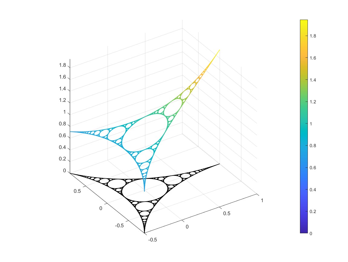
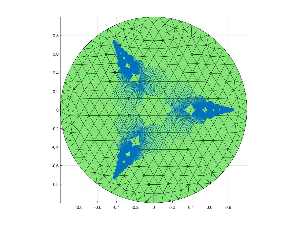
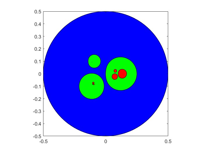
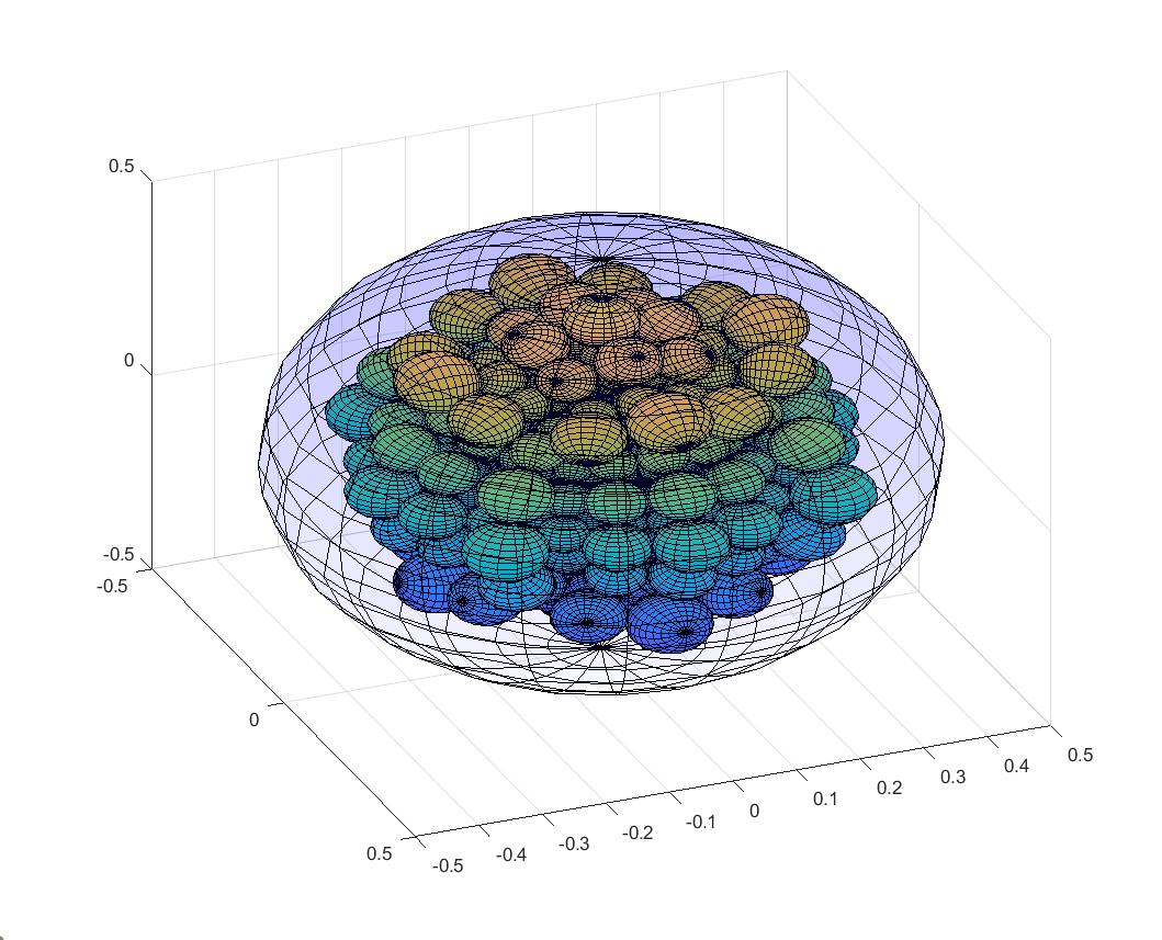
We conclude this section with a small, visual prelude to our numerical results following from this theory. Our numerical method uses approximations on to estimate the Hausdorff dimension of GDMS attractors. The corresponding approximate eigenfunctions for both the full Apollonian IFS and a truncation to its first 12 maps are shown below.
4. Derivative bounds for
In this section we will prove derivative bounds for the eigenfunctions of the Perron-Frobenius operator on maximal CGDMSs. These bounds will play a crucial role in our numerical method. We stress that, as in Section 3, the open set condition is not needed for any of the results in this section.
We start by introducing some standard notation. A multi-index is an -tuple of non-negative integers . The length of is
and we also denote
For a weakly -differentiable function , we define the operator by
As in Section 3,
will denote a maximal CGDMS and we will again assume that the sets are disjoint. Moreover, we will let
Theorem 4.1.
Let be a a finitely irreducible, maximal CGDMS in . Let , let be as in Theorem 3.6, and let be any multi-index.
-
(1)
The eigenfunctions admit real analytic extensions on .
-
(2)
If consists of Möbius maps then for any such that ,
(4.1) where .
-
(3)
If , then
(4.2) where can be any numbers such that and
Proof.
We will denote translation by by . The definition of the Möbius group implies that for all the map has the form
where ,, is an orthogonal transformation, , and
Thus,
When is not the identity we have that .
We will first prove statement (2). We fix and . For any we define a function given by
where, denotes the Euclidean norm in .
For simplicity of notation we let . Let and set . We will first show that if then
| (4.3) |
Note that if , we have nothing to prove. Therefore we may assume that
Let . Then:
and consequently
| (4.4) |
Since and
| (4.5) |
Using the Cauchy-Schwarz inequality,
| (4.6) |
Thus,
| (4.7) |
Therefore,
Since is simply connected, the analytic function
has an analytic logarithm, see e.g. [32, Lemma 6.1.10]. Thus,
is analytic for . We then let
Using Proposition 3.3 we see that for all and ,
| (4.8) |
Since the maps are analytic in , Montel’s theorem (see e.g. [38, Proposition 6]) and (4.8) imply that the maps are analytic in . Let and set
A second application of Montel’s Theorem implies that there is some subsequence and a holomorphic function such that
| (4.9) |
Therefore, Theorem 3.6 (2), (4.8) and (4.9) imply that
| (4.10) |
Note that for :
Thus, combining Theorem 3.6 (2) and (4.9) we deduce that
| (4.11) |
Recall that the polydisk metric in is defined as
A polydisk in is a set of the form
It is easy to check that
| (4.12) |
Therefore,
Recall that is holomorphic in which is an open neighborhood of . Therefore, if is any multi-index, applying the Cauchy estimates (see e.g. [38, Chapter 1, Proposition 3]), we see that
| (4.13) |
Since and were arbitrary, the proof of statement 2 is complete.
We will now prove statement 3. We fix and we define
| (4.14) |
for and . Note that for ,
| (4.15) |
Let . Recall that since the maps are conformal we have that either (when is holomorphic) or (when is antiholomorphic). By Proposition 3.3
| (4.16) |
For , define
Thus . Fix some and, without loss of generality, assume that Given any , define
To simplify notation we again let . Since is simply connected, is analytic and it does not vanish, all of the branches of are well defined on . After choosing a suitable branch, an application of Köebe’s Distortion Theorem [42, Theorem 23.1.6] gives
and
on for . Therefore is an analytic logarithm for and
| (4.17) |
for and . Therefore we can write as a power series
and by Cauchy estimates we can see that for all
| (4.18) |
Hence, if
Thus for all
| (4.19) |
Consider the complex valued function, formally defined on , given by
Note that for , the function is holomorphic in the polydisk Indeed, :
| (4.20) |
In the following we will use the embedding ,
for all . To simplify notation, we let
Note also that . Hence,
| (4.21) |
Let
For
| (4.22) |
Now note that for all
| (4.23) |
Thus,
Since the functions
are holomorphic in and the partial sums of are uniformly bounded, an application of Montel’s Theorem implies that the functions
are holomorphic in Via another application of Montel’s Theorem, we can extract a sequence of functions converging uniformly to a holomorphic function in for any . Thus, Theorem 3.6 (2) and (4.22) imply that
| (4.24) |
Moreover, Theorem 3.6 (2) and (4.23) imply that
| (4.25) |
By the Cauchy Estimates, if is any multiindex,
The proof of (3) is complete.
We will now prove (1). First observe that using (4.11) and (4.24) we can deduce that for every there exists an analytic function such that
We now set
Using Proposition 3.7, Theorem 3.9 and arguing exactly as in the proofs of (2) and (3) we can deduce that for every there exists an analytic function such that
Clearly, is real analytic on and (1) follows after we recall Theorem 3.9 (4). The proof is complete. ∎
We conclude this section with two remarks.
Remark 4.2.
5. Numerical method
In this section, we describe an algorithm that rigorously computes the Hausdorff dimension of limit sets of maximal GDMSs. The method is based on the Falk-Nussbaum approach of approximating the eigenfunctions of the Perron-Frobenius operator [16], and consists of the following steps:
-
•
Discretizing .
-
•
Approximating the Perron-Frobenius operator.
-
•
Computing upper and lower bounds for the Hausdorff dimension of the limit set.
Before we describe the method, we introduce some notation and supplementary results.
5.1. Notation and the Bramble-Hilbert lemma
Our numerical estimates apply results from finite element methods. Suppose we are working on an open, bounded domain in . Throughout the paper, we will use the usual notation for the Lebesgue (), Sobolev () and Hölder () spaces with the corresponding norms and semi-norms. Thus if , the corresponding norm is defined by
and the semi-norm by
To state the following version of the Bramble-Hilbert lemma, we recall that a domain is star-shaped with respect to if the segment
for all . Let be the space of piecewise -degree polynomials on . We will use a version of the Bramble-Hilbert Lemma with a computational constant, found in [15].
Lemma 5.1 (Explicit Bramble-Hilbert).
Suppose is an open bounded set which is star-shaped with respect to every point in a measurable set of positive measure . Let , suppose that and let If then
| (5.1) |
where
5.2. Discretizing .
To discretize we use a finite element approach. Take so that , where
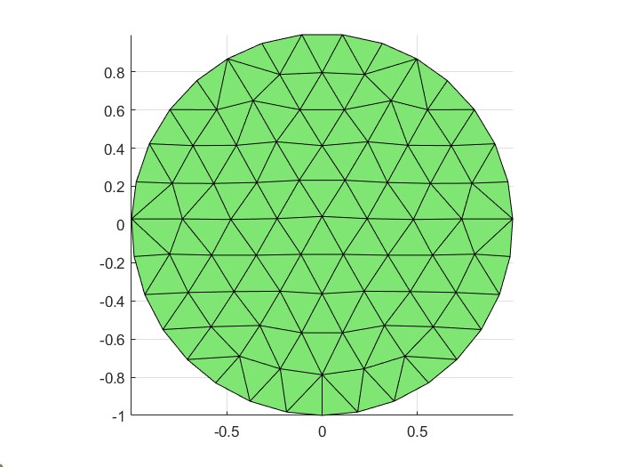
For choose a subdomain such that . We partition (triangulate) into simplices, i.e. . For simplicity we choose a conformal mesh, meaning that two neighboring simplices can intersect only by lower dimensional simplices (faces, edges, or nodes). An example of 2-dimensional conformal triangulation is shown in Figure 4.
Let and define On an element of the mesh, we define the space of linear functions on . Furthermore, let be the space of piecewise linear functions on
By the Bramble-Hilbert Lemma 5.1, for any ,
| (5.2) |
for some constant independent of , which can be explicitly estimated from the Lemma 5.1.
Remark 5.2.
Instead of triangulation, we could choose any other partition of , for example rectangular elements and use bilinear functions as was done in [18], which is a valid alternative. However, in our opinion the triangulation provides more structure that makes the implementation faster and easier.
To use the finite element space for computations, we need some basis functions. Since any element from is uniquely defined by its values at the nodes of the triangulation , we choose basis functions satisfying
and define a nodal (Lagrange) interpolation operator by
Since the nodal interpolant is invariant on , i.e. for any , and bounded from with a constant 1, by the triangle inequality, for an arbitrary , we have
Thus, we immediately obtain the following corollary.
Corollary 5.3.
Provided we have the following continuity and derivative estimates for
| (5.3) |
| (5.4) |
for some computable constants and , for any , we obtain
Thus we have
| (5.5) |
where
Thus, provides upper and lower pointwise bounds for and these bounds tend to 1 quadratically as . From now on we assume that is sufficiently small, so that
5.3. Approximating the Perron-Frobenius operator when the alphabet is finite.
Next we want to approximate the Perron-Frobenius operator which was introduced in (3.1). Recall that
Using (5.5), we have
| (5.6) |
Let be a vector with entries
and define two matrices such that
One of the technical difficulties of assembling the above matrices is to locate an element that contains . At this point, the structure of the triangulation comes very handy as one can use a barycentric point location, which makes the assembly rather efficient. For example if for the node , the image for some , then we have , where are the vertices of the simplex and , are the barycentric coordinates of the point . Thus, we obtain the contribution to the entries of -th columns of the matrices and the rows corresponding to the global indices of the nodes weighted by the barycentric coordinates . This step can be vectorized for all , making the assembly very efficient.
5.4. Computing upper and lower bounds of the Hausdorff dimension
The matrices consist of non-negative entries and we can use the following key result for such matrices [18, Lemma 3.2].
Lemma 5.4.
Let be an matrix with non-negative entries and an -vector with strictly positive components. Then,
where denotes the spectral radius of .
Since
where denotes the spectral radius of , for all ,
and
Therefore Lemma 5.4 implies that
Let and recall by Bowen’s formula from Section 2 that . Thus, our goal is to compute tight upper and lower bounds such that . Since the map is strictly decreasing, if we find such that , then and as a result . Similarly, if we find such that , then and as a result . In conclusion, we would have , which is a rigorous effective estimate for the Hausdorff dimension of the set .
Thus, given matrices and the problem essentially reduces to nonlinear problem of computing a parameter that corresponds to a leading eigenvalue . Since there is a spectrum gap between the leading eigenvalue and the rest, this problem is well-suited for a power method, which starting from arbitrary vector , generates an iterative sequence given by
and the corresponding sequence of numbers is given by
such that and converges to the corresponding eigenvector at the rate . Since , the power method is rather efficient. Furthermore, since the power method only requires matrix-vector multiplication, there is no need to construct the matrices and explicitly, which is an important issue for large problems, for example in 3D.
Using the logarithm, the above nonlinear problem is equivalent to root finding problem. There are many good choices can be used. In our computations, we used a variation of a secant method, since good initial guesses for such problem are available.
5.5. Case of infinite alphabet
In the case of the infinite alphabet, we consider the truncated finite alphabet and initially define the matrices on the truncated alphabet as,
For estimating the lower bound , we can use the matrix , however for estimating the upper bound , we need to modify the matrix to account for the tail
Provided that
converges uniformly in , in view of the continuity estimate (5.3), we have that for any
Thus, for each column of we only need to modify the first row of . In the above estimate, the choice of is arbitrary, we could select any other node (or nodes) as well. The exact estimate of the constant , depends of course on a concrete problem and the size of . In many examples, we can chose the size of the truncated so large that the modified matrix allows us to obtain a sharp upper bound .
Remark 5.5.
In the case of infinite alphabet, We have two sources of errors, one is due to discretization of the domain and the other is due to truncation of the alphabet . The sizes of the matrices and only depend on the discretization parameter and not on the truncated alphabet . The size of the truncation alphabet affects of course the entries of the matrices and and the time it takes to assemble them. However, as we already mentioned in the section 5.3, this step can be made very efficient and in all our examples given below, we are able to take so large (corresponding to be very small) that the dominating error is due to the discretization parameter only.
5.6. Mesh Trimming
In this section we provide a meshing scheme for fractals generated by CGDMSs, that eliminates computationally redundant points in the iterative creation of the mesh and some cases can reduce the number of degrees of freedom by orders of magnitude. We visualize the method using the Apollonian gasket, although the algorithm is presented below works for general CGDMS.
In section 5.3, we showed that elements of the approximating matrices are defined by the expression
| (5.7) |
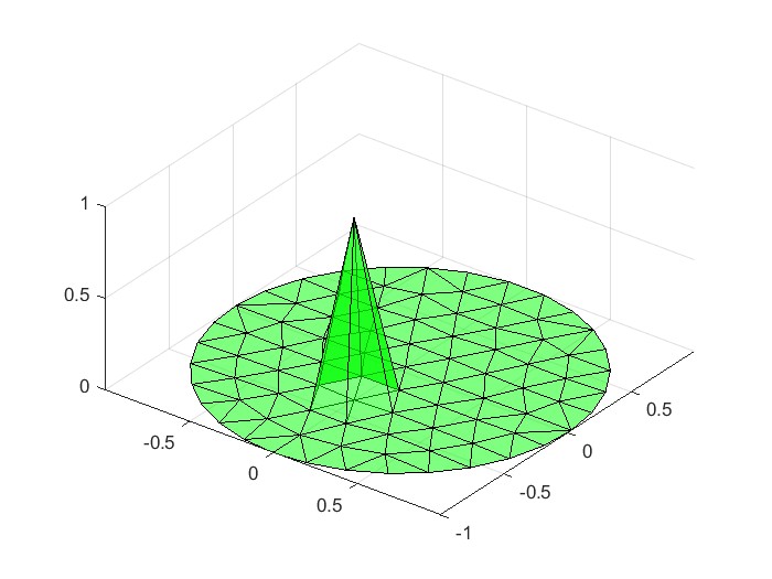
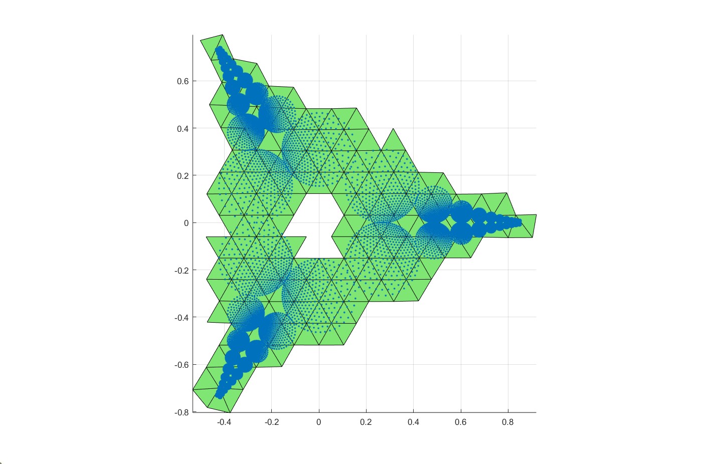
Looking at Figure 6, which shows a general mesh on and the image of all the nodes under the map as blue dots, one can see that the blue dots are not distributed uniformly. In fact most of the elements (triangles) do not contain any such dots. This implies that when we generate the matrices using formula (5.7), the resulting matrices will have many zero columns. Such columns do not play any role in computing the corresponding eigenvectors, and the size of the matrix can be significantly reduced by removing those zero columns and the corresponding rows. Alternatively, we could just remove those elements altogether at the beginning, see the in the mesh on Figure 6, which significantly saves time for generating the approximating matrices.
Remark 5.6.
The step 3 for unstructured meshes may be computationally difficult, however, if the meshes consist of shape regular simplices this step can be done directly using the edge data structure.
6. Applications
In this section, we illustrate how the method can be applied to various CGDMSs. In particular, we verify that these systems are indeed CGDMSs and highlight some properties of the general families that these systems belong to. In Section 6 we will describe the specific implementation of our numerical method for these examples.
6.1. -dimensional continued fractions
In this section we review -dimensional continued fractions and some of their dynamical properties. We find their -number and prove they are a CIFS.
Definition 6.1 (-dimensional Continued Fractions IFS).
Let and let denote the Euclidean norm. The -dimensional continued fraction IFS, denoted , consists of the maps
| (6.1) |
where
To verify that is a CIFS, first note that . We are left with three properties to check. First, the the system has to satisfy the OSC. Second, each must map to itself to be an IFS. Finally, there must exist an open set furnishing a conformal extension for each .
Lemma 6.2.
For any with ,
Proof.
Each in is the composition of two distinct maps — a translation followed by an inversion about the unit sphere:
-
(1)
and
-
(2)
Since , we see that for distinct
Applying the injectivity of an inversion,
so the open set condition is satisfied. ∎
We now provide an analytic proof that each maps to itself, proving that is an IFS.
Lemma 6.3.
For each , .
Proof.
It suffices to show that for all ,
Since , for all , ,
Dividing through by and squaring both sides gives
From here, subtracting terms yields
Equating
and taking square roots, we see that
∎
We are interested in the existence and maximality of conformal extensions of . The existence of a conformal extension shows that is a CIFS, while finding maximal extensions is needed for eigenfunction bounds. Introducing some notation, for all , let
To show the existence of a uniformly contracting conformal extension we must find a so that
Note that in this lemma, we only consider corresponding to words of finite length greater than one, as it is not true for single letters (specifically, letting , we see that whenever ). While this formally corresponds to a different dynamical system, they clearly share the same limit set.
Lemma 6.4.
For any ,
where .
Proof.
To show this, note that since , it suffices to show that for any . Consider the set
We wish to show that . To do so, note that the boundary of is a half plane, and thus described uniquely by points. If we can show that , we will be done.
By properties of Möbius transformations, we know that is either a sphere or a hyperplane. Notably, any points determine this image. For the point at infinity, . Moreover, . Now, let , be the point . Certainly for each , as
so our claim is proven.
Defining the set
note that the first coordinate of any point in is always positive when . Hence for any and any , , so , verifying our claim. Note also that this inequality is strict, for if then , and is undefined. ∎
Hence we have shown that -dimensional continued fractions are a CIFS. We now move onto tail bounds for these systems for continued fraction systems in any dimension.
Lemma 6.5 (Tail Bounds).
Let . Then for any ,
| (6.2) |
where is the surface area of the sphere of radius and
Proof.
Consider . From the definition of , we immediately have
In addition, by the Mean Value Theorem and the derivative estimate (4.1) with , we have
and as a result
| (6.3) |
for any . To estimate the sum we use the integral comparison test. Using that for any and any ,
we have
Using the spherical coordinates , we compute
Combining, we obtain the result.
∎
Remark 6.6.
Following the lines of more refined analysis from [17], we could obtain a slightly sharper tail bounds. However, the above bounds are more than sufficient for our purpose, and the dominating error is due to discretization of .
6.2. Quadratic perturbations of linear maps (abc-examples)
In this section we discuss a CIFS in the the complex plane which does not consist of Möbius maps. Suppose that and let
for The corresponding (formal) CIFS is denoted by An arbitrary set of such maps will not be a CIFS. The maps may not be contractions, have intersecting images, or be non-invertible. Conformality is automatic, so for verification purposes we need to do the following:
-
(1)
Verify the maps are contractions on .
-
(2)
Find an open, connected set for which each extends to a uniformly contracting map taking into itself.
-
(3)
Verify the OSC holds on .
-
(4)
Verify the Bounded Distortion Property.
Many of these questions may be verified using computational means, provided the system satisfies appropriate separation properties. An investigation of these algorithms is beyond the scope of the paper, and instead we show how to verify this is a CIFS in one particular case. In particular, consider the CIFS consisting of the maps
defined on with . To show this system maps to itself we use norm estimates. For all we have that
implying
for all Hence for all . To verify the OSC, simply note that for all . Pairing this with the fact that for all , it is obvious that for all . More explicitly, we have that
Checking case by case, we find that
-
(1)
For and ,
so and are disjoint.
-
(2)
For and ,
so and are disjoint.
-
(3)
For and ,
so and are disjoint.
Hence our system satisfies the OSC. To find an open set satisfying property 3, recall that
we wish to find the supremum of for which whenever . For an arbitrary , taking the supremum norm on yields
we must solve
Doing so, we have that
Hence for this example.
Moving onto injectivity, it is sufficient to show the existence of a nonzero directional derivative for some direction. In particular, taking derivatives yields
Since we have that
so injectivity has been proven. Of course, since the alphabet is finite, the tail bounds are not needed.
6.3. An application to Schottky groups
Another application of our estimates it to 2D Schottky Groups, specifically classical, nonhyperbolic Schottky Groups generated by Möbius transformations. Suppose that , , are disjoint closed disks in , and consider Möbius transformations of the form
For each , is a contraction on its domain of definition. However, this is not yet a CGDMS as it does not satisfy the open set condition. To rectify this, consider the maps
all of which are defined when . The incidence matrix is then just a matrix of ’s whenever , and zeros everywhere else. Moreover, extending to the whole Riemann Sphere, it is apparent that only when , so uniform contractivity follows from the finiteness of the system. We now provide a specific example of a Schottky group for which our theory applies. Consider the initial, paired balls
Visually, these circles are shown below:
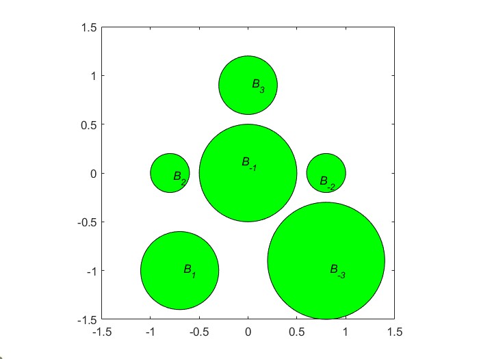
The mappings between them were found computationally and are certainly not unique. Because of this, Schottky groups give a great example CGDMSs whose 1-cylinder sets agree but whose limit sets have different Hausdorff dimension. The maps used in this paper are as follows:
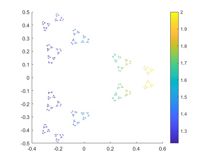
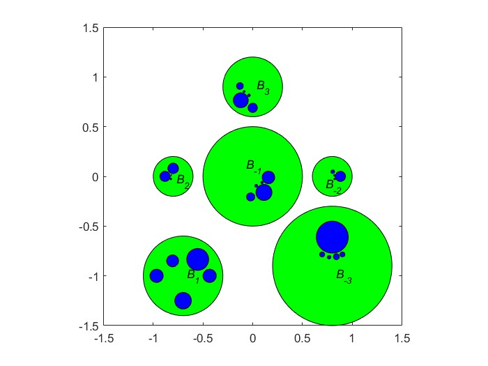
A graphic representing the first iteration is in Figure 11.
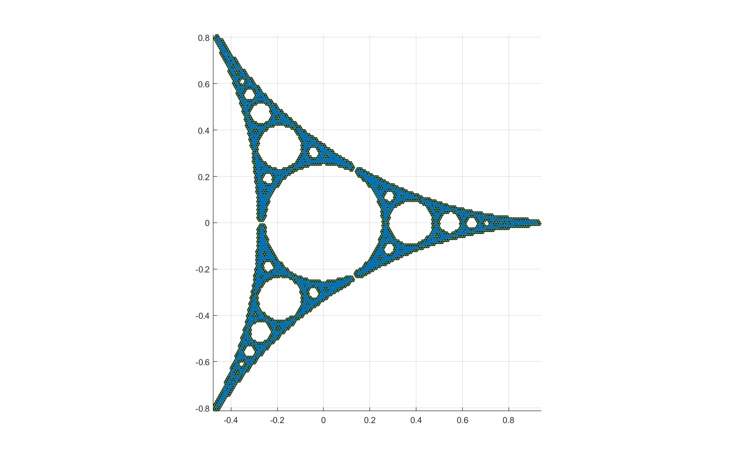
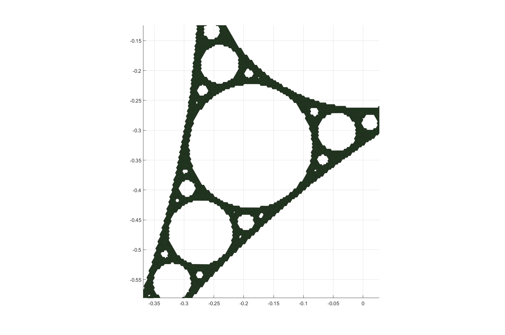
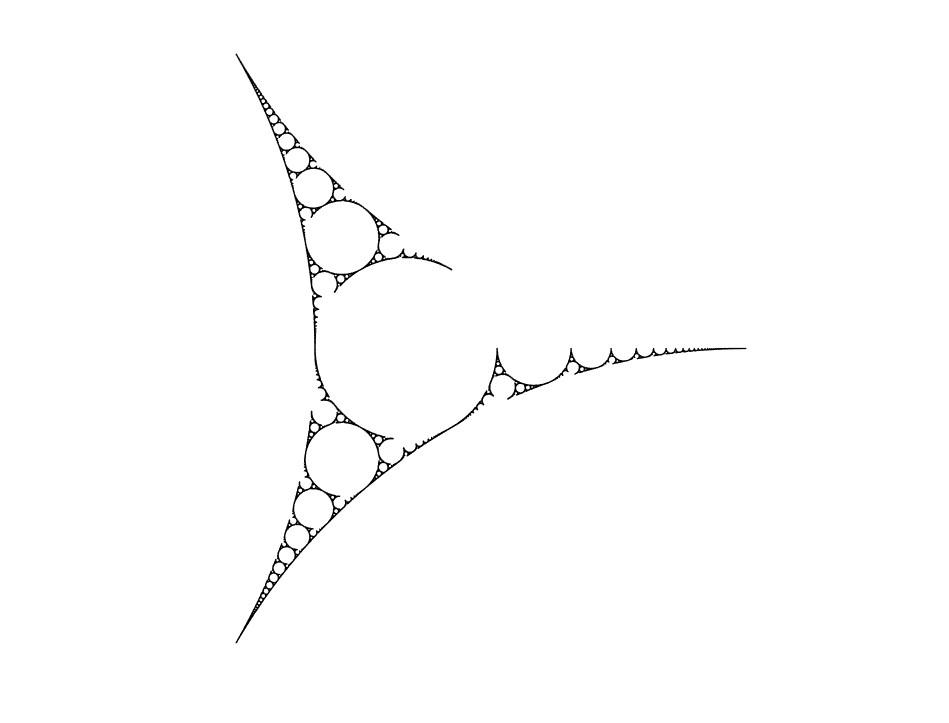
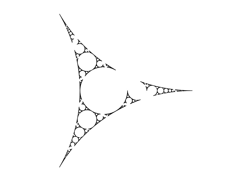
6.4. The Apollonian gasket
We now focus our attention on one of the most famous fractals, the Apollonian packing. To fully describe the packing as the limit of a conformal IFS, suppose that and consider the angles
The generators of the system then have a representation via the maps
where is the standard complex rotation by angle . With this notation, the infinite set of maps generating the Apollonian packing is
where
For the rest of this section, we let .
Proposition 6.7 ().
The maximal domain furnishing a conformal extension for the Apollonian IFS is .
Proof.
We will show that with satisfies . Writing
consider the matrix representation of , given by
Notice that
as is the single eigenvalue of multiplicity 2 for . By nilpotence
and so the matrix representation of is
Using this representation, and the matrix representation for the rotation
we see that the map
has the matrix representation given by
| (6.4) |
Now we consider the action of each map on . Start with the image of . Since is a pole of , maps the ball onto the right part of the plane of the vertical line
This is easy to see, for
and
The equality follows by noticing that the real parts of both these points are equal.
This is followed by a rotation by — that is, finding the image after . By the symmetry of the gasket maps under the complex conjugation, we will only need to consider a rotation by . Under the rotation , the line becomes
Solving for real and imaginary parts to be zero, we see that the new line passes through the points and .
The image after is given by the inversion by . This is a Möbius transformation, so it maps the line into a circle. To compute the center and the radius of this circle, notice that
Thus, we need to compute the center and radius of circle passing through three points , , and , which is equivalent of solving a linear system with the matrix
and the right hand side
Solving, we obtain that the desired center of the circle is and the radius .
The image after is simply the translation by , corresponding to the matrix
Alternatively, this is the map , which is just a translation by and the new image is just a circle centred at of radius . We can represent it as
We could now proceed with the next map , but we will use a different approach. Due to the elementary fact that for functions and , implies , a splitting argument for may be used to show that . Here the map is the map corresponding to the product of matrices
and the map to the product of matrices
Naturally the rotation leaves invariant. Since
we need to find the image of under the Möbius map We proceed similarly when we treated , consider the image of three points , , and .
Thus, we need to compute the center and radius of circle passing through three points , , and , which is equivalent to solving a linear system with the matrix
and the right hand side
with . Solving, we obtain that the center of the circle is and the radius is .
To conclude , we only need to establish that the distance between centers of the circles and is greater than the sum of the radii and . Magically,
and the direct computations show that even for ,
and of course the above distance is even greater for . ∎
Remark 6.8.
The decomposition in (6.4) is also of practical interest. If one were to naively compute for higher powers of (specifically, for ) the entries of would become so large they could not be stored in memory. Using the fact that Möbius maps act on , the scaling factor outside of the decomposition of may be ignored, avoiding the aforementioned exponential scaling.
6.4.1. Tail Bounds
In this section we find tail bounds for the Apollonian gasket. As mentioned with continued fractions, such bounds are necessary for rigorous Hausdorff dimension estimates of infinite systems, though the structure of such bounds will change depending on the system. Generally, an ordering needs to be given on the maps of the system, which in this case is given in it’s definition.
Recall that any Möbius transformation
has a matrix representation
and the norm of its derivative at is given by the formula
| (6.5) |
As in the previous section, the matrix form for is
Finding tail bounds for the system will amount to applying (6.5) and the chain rule. Focusing on the rightmost matrices, note that is just a rotation by , and thus leaves the derivative unchanged. Taking the determinant,
The and terms for the map are and , respectively, so the derivative will be maximized when
is minimized. This is at , giving the derivative . Hence we have that
We need to find . Since is symmetric about the real axis, the points
are antipodal points on . Thus Without loss of generality, suppose that . Then rotating by gives
Moving onto the next three maps, note that the final map is just a rotation by , and therefore doesn’t change the norm of the derivative. Hence we can omit it from our calculations. Furthermore,
implying that
Referring back to (6.5), this implies that
Notice that the above maximum occurs at that minimizes
It is well known from basic complex analysis that the minimum of on the circle is attained for
with , , and , we have
Using that , we compute,
After a simple application of the integral comparison test, one finds that
7. Hausdorff dimension estimates
In this section, for the concrete example from the previous section, we provide the estimates for all the constants and parameters needed for computations and give reliable computational range the Hausdorff dimensions.
7.1. 2-dimensional continued fractions
In two dimensions , hence
and as a result and by Bramble-Hilbert Lemma 5.1
By Theorem 4.1, for any , and taking ,
| (7.1) |
Thus, we need to obtain an estimate for which depends on the Hausdorff dimension of the limit set. Although we do not know this exactly, good upper bounds on the quantity can be applied.
7.1.1. Alphabet with four smallest generators.
For a simple illustration we consider the alphabet consisting with four generators,
Denoting the limit set of the system by , the upper bound for the is . As a result
combining the estimates we obtain
Naturally, no tail bounds are required in this case. Using this estimate, we compute that
7.1.2. Infinite lattice alphabet.
Now we consider the infinite alphabet . For this example, we know that and as a result
combining, we obtain
For tail bound we use Lemma 6.5. Thus, since for ,
we have
and to account for the tail, we need modify -th column and the row of the matrix that corresponds to the zero node.
Denoting the limit set of this system by , our computation found that
7.1.3. Gaussian prime alphabet.
As an intermediate example, we consider the case when the alphabet consist of Gaussian prime with positive real parts. For this example, we know that and as a result
combining, we obtain
For tail bound we use Lemma 6.5. Thus, since for ,
we have
and to account for the tail, we need modify -th column and the row of the matrix that corresponds to the zero node.
Denote the limit set of this system by . Then,
7.2. -dimensional continued fractions
In three dimensions , hence
and as a result and by Bramble-Hilbert Lemma 5.1
By Theorem 4.1, for any , and taking ,
| (7.2) |
7.2.1. Alphabet with five smallest generators.
First, we consider the alphabet consisting with five generators,
Denoting the limit set of the system by , the upper bound for the is . As a result
combining the estimates we obtain
Naturally, no tail bounds are required in this case. Using this estimate, we compute that
7.2.2. Infinite lattice alphabet.
Now we consider the infinite alphabet . For this example, we know that and as a result
combining all estimates we obtain
To account for the tail bound, similarly to 2D case, we use Lemma 6.5. Thus, since for ,
we have
and again to account for the tail, we need modify -th column and the row of the matrix that corresponds to the zero node.
Suppose that is the limit set for the above 3-dimensional continued fraction system. Using a mesh size of we found that
7.3. Quadratic perturbations of linear maps
Similarly to Section 7.1, and by Bramble-Hilbert Lemma 5.1
However, since this system does not consist of Möbius transformations, to estimate we will use (3) from Theorem 4.1, namely
| (7.3) |
where , can be any numbers such that and . Since ,
Setting and , we need to optimize the expression
As before, this varies depending on the parameter we are using. Setting , an upper bound for our system, we find that
for all . Combining this with the Bramble-Hilbert Lemma, we see that
For our computations, we used a mesh of size . Denoting the limit set by , a resulting computation gave
This is up to standard MATLAB long precision and may be given as an equality, due to the computed upper and lower bounds being equal. Expanding the precision of the computation would therefore yield more digits.
7.4. Schottky groups
Error estimates for 2-dimensional, classical Schottky groups are slightly different than continued fractions. Since we are in two dimensions, implying . However, the optimization problem involving will necessarily change, as in many cases. The corresponding minimization problem then is
Note that can become arbitrarily small, implying different bounds are needed for these cases. In the provided example, it is straightforward to verify that . The subsequent minimization is
This, like the other minimization, is changed for each we consider. That said, since an upper bound on the dimension of our Schottky group is 0.78, one finds that
Completing our bounds, just recall (4.1), and so
Denote the limit set of the Schottky group by . Then
The maximum mesh size used for this computation was .
7.5. Apollonian gasket
The bounds for the Apollonian packing are similar to those on complex continued fractions. Since the generating IFS consists of Möbius maps, the bounds from the Bramble-Hilbert Lemma remain the same. Specifically, we have that so
Applying (4.1), we need to optimize the expression
when and is an upper bound for the Hausdorff dimension of . Since , one finds that
Excluding the tail, we find that
Adding in the tail bounds,
As shown below, similar bounds will hold for each subsystem we consider. For the limit set of the Apollonian gasket, we have that
This bound was obtained using a mesh of size .
7.5.1. A Finite Apollonian Subsystem
The first subsystem of the Apollonian gasket we consider is a finite subsystem consisting of the first 12 maps in it’s standard enumeration. In particular, this is given by
with corresponding limit set . A visual of a system and its corresponding eigenfunction is found at the end of section 3 2. This system exhibits our methods capabilities to estimate systems without the quadratic decaying tails seen in other examples. As such, the bounds for it are similar to the original gasket. In this case, , so optimizing the expression yields
and so the Bramble-Hilbert lemma implies
Using a mesh size of , our numerics found that
7.5.2. The Packing without a Generator
Due to the flexibility of our method, we can find rigorous Hausdorff dimension estimates for infinite subsystems of the Apollonian gasket. Starting with one of the simplest subsystems, we consider the fractal generated from the Apollonian gasket without a generator. Specifically, let
with corresponding limit set . Being a subsystem, all of the previous bounds carry over. In this case, taking one finds
and hence, excluding the tail
The appropriate tail bounds in this situation are
Moving onto our numerics, using a mesh size of we found that
7.5.3. The Packing without a Spiral
Another interesting subsystem of occurs when a map from a different generator is removed for each level . Taking from concurrent maps, this yields a spiral of disks taken away from the fractal. Specifically, consider the CIFS
It is clear that the tail bounds for this system are the same as in the previous example, being
where if and only if . The specific eigenfunction bounds differ at a certain level due to the higher dimension of the limit set for compared to the system missing a generator. In this case , which is close enough to 1.24 so that the same full bound applies
Denote the limit set of this system by . Then our numerics find that
with mesh size .
References
- [1] Zai-Qiao Bai and Steven R. Finch. Precise calculation of Hausdorff dimension of Apollonian gasket. Fractals, 26(4):1850050, 9, 2018.
- [2] Jean Bourgain and Alex Kontorovich. On Zaremba’s Conjecture. Ann. of Math., Vol. 180, 137-196, 2014.
- [3] Rufus. Bowen. Hausdorff dimension of quasicircles. Inst. Hautes Études Sci. Publ. Math., (50):11–25, 1979.
- [4] David W. Boyd. The residual set dimension of the Apollonian packing. Mathematika, 20:170–174, 1973.
- [5] Richard T. Bumby. Hausdorff dimension of sets arising in number theory. In Number theory (New York, 1983–84), volume 1135 of Lecture Notes in Math., pages 1–8. Springer, Berlin, 1985.
- [6] Ruchart T. Bumby. Hausdorff dimensions of Cantor sets. J. Reine Angew. Math., 331:192–206, 1982.
- [7] Vasileios Chousionis, Dmitriy Leykekhman, and Mariusz Urbański. The dimension spectrum of conformal graph directed Markov systems. Selecta Math. (N.S.), 25(3):Paper No. 40, 74, 2019.
- [8] Vasileios Chousionis, Dmitriy Leykekhman, and Mariusz Urbański. On the dimension spectrum of infinite subsystems of continued fractions. Trans. Amer. Math. Soc., 373(2):1009–1042, 2020.
- [9] Vasileios Chousionis, Jeremy Tyson, and Mariusz Urbański. Conformal graph directed Markov systems on Carnot groups. Mem. Amer. Math. Soc., 266(1291):viii+155, 2020.
- [10] Thomas W. Cusick. Continuants with bounded digits. Mathematika, 24(2):166–172, 1977.
- [11] Thomas W. Cusick. Continuants with bounded digits. II. Mathematika, 25(1):107–109, 1978.
- [12] Thomas W. Cusick. Continuants with bounded digits. III. Monatsh. Math., 99(2):105–109, 1985.
- [13] Tushar Das and David Simons. Exact dimensions of the prime continued fraction cantor set. preprint, arXiv 2305.11829, 2023.
- [14] Tushar Das, Giulio Tiozzo, Mariusz Urbański, and Anna Zdunik. Open Dynamical Systems: Statistics, Geometry, and Thermodynamic Formalism. De Gruyter Expositions in Mathematics. to appear.
- [15] Ricardo G. Durán. On polynomial approximation in Sobolev spaces. SIAM Journal on Numerical Analysis, 20(5):985–988, 1983.
- [16] Richard S. Falk and Roger D. Nussbaum. eigenfunctions of perron-frobenius operators and a new approach to numerical computation of hausdorff dimension, 2016.
- [17] Richard S. Falk and Roger D. Nussbaum. Eigenfunctions of Perron-Frobenius Operators and a New Approach to Numerical Computation of Hausdorff Dimension: applications in . J. Fractal Geom., Vol. 5, 2016.
- [18] Richard S. Falk and Rorger D. Nussbaum. A New Approach to Numerical Computation of Hausdorff Dimension of Iterated Function Systems: Applications to Complex Continued Fractions. Integral Equations Operator Theory, 90(5):90–61, 2018.
- [19] Irving J. Good. The fractional dimensional theory of continued fractions. Proc. Cambridge Philos. Soc., 37:199–228, 1941.
- [20] D. Hensley. A polynomial time algorithm for the Hausdorff dimension of continued fraction Cantor sets. J. Number Theory, 58(1):9–45, 1996.
- [21] Doug Hensley. The Hausdorff dimensions of some continued fraction Cantor sets. J. Number Theory, 33(2):182–198, 1989.
- [22] Doug Hensley. Continued fractions. World Scientific Publishing Co. Pte. Ltd., Hackensack, NJ, 2006.
- [23] Doug Hensley. Continued fractions, Cantor sets, Hausdorff dimension, and transfer operators and their analytic extension. Discrete Contin. Dyn. Syst., 32(7):2417–2436, 2012.
- [24] ShinnYih Huang. An improvement to Zaremba’s conjecture. Geom. Funct. Anal., 25(3):860–914, 2015.
- [25] John E. Hutchinson. Fractals and self-similarity. Indiana Univ. Math. J., 30(5):713–747, 1981.
- [26] Vojtěch Jarnik. Zur metrischen theorie der diophantischen approximationen (on the metric theory of diophantine approximations). Prace Matematcyzno-Fizyczne, 36, 1928-1929.
- [27] Oliver Jenkinson. On the density of Hausdorff dimensions of bounded type continued fraction sets: the Texan conjecture. Stoch. Dyn., 4(1):63–76, 2004.
- [28] Oliver Jenkinson and Mark Pollicott. Computing the dimension of dynamically defined sets: and bounded continued fractions. Ergodic Theory Dynam. Systems, 21(5):1429–1445, 2001.
- [29] Oliver Jenkinson and Mark Pollicott. Rigorous Effective bounds on the Hausdorff dimension of continued fraction Cantor sets: A hundred decimal digits for the dimension of . Adv. in Math. 325, 87 - 115, 2018.
- [30] Oliver Jenkinson and Mark Pollicott. Rigorous dimension estimates for Cantor sets arising in Zaremba theory. In Dynamics: topology and numbers, volume 744 of Contemp. Math., pages 83–107. Amer. Math. Soc., [Providence], RI, [2020] ©2020.
- [31] Janina Kotus and Mariusz Urbański. Meromorphic dynamics. Vol. I. Abstract ergodic theory, geometry, graph directed Markov systems, and conformal measures, volume 46 of New Mathematical Monographs. Cambridge University Press, Cambridge, 2023.
- [32] Steven G. Krantz. Function theory of several complex variables. AMS Chelsea Publishing, Providence, RI, 2001. Reprint of the 1992 edition.
- [33] M. Ju. Ljubich. Entropy properties of rational endomorphisms of the Riemann sphere. Ergodic Theory Dynam. Systems, 3(3):351–385, 1983.
- [34] R. Daniel Mauldin and Mariusz Urbański. Dimensions and measures in infinite iterated function systems. Proc. London Math. Soc. (3), 73(1):105–154, 1996.
- [35] R. Daniel Mauldin and Mariusz Urbański. Dimension and measures for a curvilinear Sierpinski gasket or Apollonian packing. Adv. Math., 136(1):26–38, 1998.
- [36] R. Daniel Mauldin and Mariusz Urbański. Graph directed Markov systems, volume 148 of Cambridge Tracts in Mathematics. Cambridge University Press, Cambridge, 2003. Geometry and dynamics of limit sets.
- [37] Curtis McMullen. Hausdorff Dimension and Conformal Dynamics, III : Computation of Dimesion. American Journal of Mathematics, Vol. 120, 691-721, 1997.
- [38] Raghavan Narasimhan. Several complex variables. Chicago Lectures in Mathematics. University of Chicago Press, Chicago, Ill.-London, 1971.
- [39] Mark Pollicott and Mariusz Urbański. Asymptotic counting in conformal dynamical systems. Mem. Amer. Math. Soc., 271(1327):v+139, 2021.
- [40] Mark Pollicott and Polina Vytnova. Hausdorff dimension estimates applied to Lagrange and Markov spectra, Zaremba theory, and limit sets of Fuchsian groups. Trans. Amer. Math. Soc. Ser. B, 9:1102–1159, 2022.
- [41] Mariusz Urbański, Mario Roy, and Sara Munday. Non-invertible dynamical systems. Vol. 2. Finer thermodynamic formalism—distance expanding maps and countable state subshifts of finite type, conformal GDMSs, Lasota-Yorke maps and fractal geometry, volume 69.2 of De Gruyter Expositions in Mathematics. De Gruyter, Berlin, [2022] ©2022.
- [42] Mariusz Urbański, Mario Roy, and Sara Munday. Non-invertible dynamical systems. Vol. 3. Analytic endomorphisms of the Riemann sphere, volume 69.3 of De Gruyter Expositions in Mathematics. De Gruyter, Berlin, [2023] ©2023.
- [43] Polina Vytnova and Caroline Wormell. Hausdorff dimension of the apollonian gasket. arXiv:2406.04922, 2024.