A magnetised Galactic halo from inner Galaxy outflows

Large-scale magnetic fields are observed off the midplanes of disk galaxies, indicating that they harbour magnetised halos[1, 2]. These halos are crucial to studies of galaxy evolution, galactic-scale outflows, and feedback from star formation activity[3, 4, 5]. Identifying the magnetised halo of the Milky Way is challenging because of the potential contamination from foreground emission arising in local spiral arms[6, 7]. Additionally, it is unclear how our magnetic halo is influenced by recently revealed large-scale structures such as the X-ray emitting eROSITA Bubbles[8], which, according to previous simulations, might be transient structures powered by the Galactic Center[9, 10] or the Galaxy’s star-forming ring[11]. Here we report the identification of several kpc-scale magnetised structures based on their polarized radio emission and their gamma-ray counterparts, which can be interpreted as the radiation of relativistic electrons. These non-thermal structures extend far above and below the Galactic plane and are spatially coincident with the thermal X-ray emission from the eROSITA Bubbles. The morphological consistency of these structures suggests a common origin, which can be sustained by Galactic outflows driven by the active star-forming regions located at $3-5$ kpc from the Galactic Centre. These results reveal how X-ray-emitting and magnetised halos of spiral galaxies can be related to intense star formation activities and suggest that the X-shaped coherent magnetic structures observed in their halos can stem from galaxy outflows.

Main

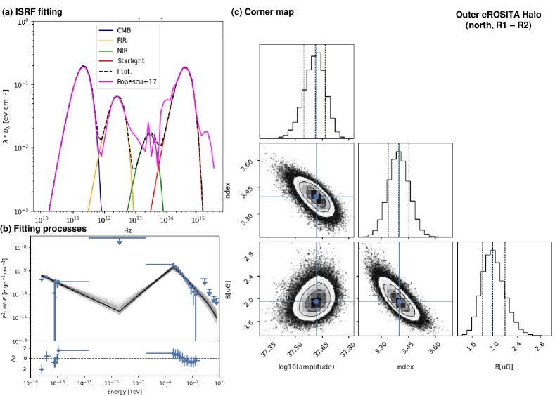
Figure 1: Supplementary Figure 1 $\mid$ The fitting details for northeastern outer outflows. These calculations correspond to the SED fitting in Figure 2c for the patch R1 - patch R2. (a) the seed photon field through the fitting of the ISRF+CMB from [Ref. [83]]. (b) The fitting processes for the MCMC fitting (different grey lines) and the data deviation ($\Delta\sigma$) compared to the best fit. The data dispersion is within 2-$\sigma$ to the best fit. (c) the corner map for the MCMC fitting. The Gaussian distribution for all the three parameters have been reached.

X-ray-emitting galactic halos have been discovered in star-forming galaxies[12, 13]. Several of them are accompanied by large-scale coherent magnetic structures revealed by radio data[14, 2]. However, the relationship between the X-ray-emitting and magnetised galactic halos is unclear, and similarly for their nature and origins. The recent discovery of the X-ray emitting large structures of the Milky Way, the eROSITA Bubbles[8], provides important physical insights to our understanding of galactic halos. Figure 1 compares the eROSITA all-sky emission at 0.6-1.0 keV with the magnetic field determined from the polarized synchrotron emission at 22.8 GHz from WMAP[15], for which Faraday rotation effects are marginal. Several magnetic structures revealed through their polarized emission and coherent field line direction, here denoted as magnetic ridges, appear in the inner Galaxy, emerging from the Galactic plane[16] and stretching for more than 20^∘. The polarized intensity is enhanced at the edges of the eROSITA Bubbles. The magnetic field directions are parallel to the Bubbles’ edges in the east. The magnetic ridges show a general tilt westwards, starting from the disc and rising to high latitudes. This implies a potential connection between magnetic ridges and the eROSITA Bubbles.

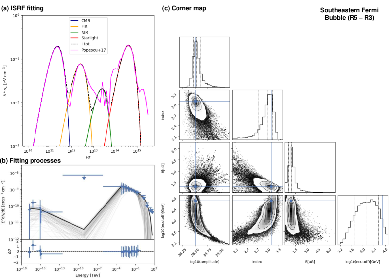
Figure 3: Supplementary Figure 3 $\mid$ The fitting details for southeastern cap of the Fermi Bubble. Same as Supplementary Figure 1 but for the SED fitting in Figure 2e for the patch R5 - patch R3. The data dispersion is within 2-$\sigma$ to the best fit. The Gaussian distribution for all the four parameters have been reached.

A key issue for these extended structures is whether they are local objects within the Local hot Bubble (LB)[17], or distant Galactic structures. Thus far, they have mostly been modeled as shells of old supernova remnants in the LB[18, 16]. Extended Data Figure 3, panels a-d, reveal an anti-correlation between the X-ray maps of eROSITA[8] (0.6–1.0 keV) at mid/low Galactic latitudes and the dust column density based on the dust distribution within 500 pc from the Sun by [Ref.[19]]. Therefore, the local dust within 500 pc is responsible for the X-ray absorption, implying that the X-ray emitting eROSITA Bubbles are not local and the bulk of the emitting structures must originate from a distance beyond the 500-pc of our Local Arm.

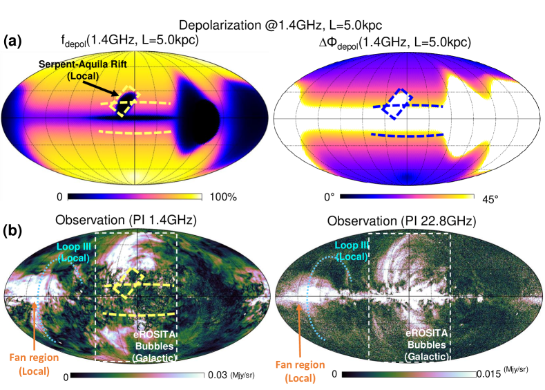
Figure 5: Extended Data Figure 5 $\mid$ Depolarization of the radio polarized emission ridges and local structures, such as the Fan region and Loop III. (a) Depolarization analyses ($f_{depol}$, $\Delta\Phi_{depol}$) at 1.4 GHz; (b) observations for polarized intensity at 1.4 GHz[29, 50] and 22.8 GHz[15, 52]. No Faraday depolarization is expected for local emission down to the Galactic disc. At 1.4 GHz, the radio counterpart of the eROSITA Bubbles is depolarized at Galactic latitudes smaller than $|b|\lesssim 20^{\circ}$, whilst no depolarization is observed for the Fan region or Loop III.

We also estimate our distance from the polarized synchrotron emission of the magnetised ridges thanks to the Faraday-rotation depolarization of the foreground turbulent magnetised medium[20, 21, 22] (see Methods and Extended Data Figures 3–5). The depolarization is largest at lower frequencies and decreases at higher latitudes because of a decline with latitude of the magnetic field strength and electron density in the foreground medium. Using the depolarization expected from the magneto-ionic medium out to different depths, we find that the observed depolarization is consistent with that produced by the medium out to distances of several kpc (Extended Data Figure 4). The polarized magnetic ridges thus are several kpc-scale Galactic structures. This indicates that the bulk of the emission associated with the North Polar Spur (NPS) is beyond several kpc from us, however it does not exclude a smaller contribution from some local features.

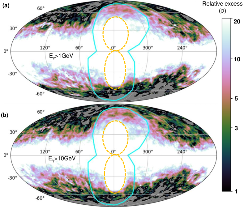
Figure 6: Extended Data Figure 6 $\mid$ $\gamma-$ray diffuse emission intensity maps. Following Figure 2a and the calculations in Methods, we calculate the relative excess of the $\gamma-$ray flux density comparing to the patch R0 for $\gamma-$ray photons with (a) $E_{\gamma}\gtrsim 1$ GeV; (b) $E_{\gamma}\gtrsim 10$ GeV. The background area is selected in the yellow triangle in the northeast. The northern edges of the eROSITA Bubble are consistent with $\sigma\gtrsim 5$, the same as $E_{\gamma}\gtrsim 100$ GeV. However, there is no clear counterpart of diffuse gamma-ray emission to the southern eROSITA Bubble, unlike the southern cut shown at Extended Data Figure 8 for $E_{\gamma}\gtrsim 100$ GeV.

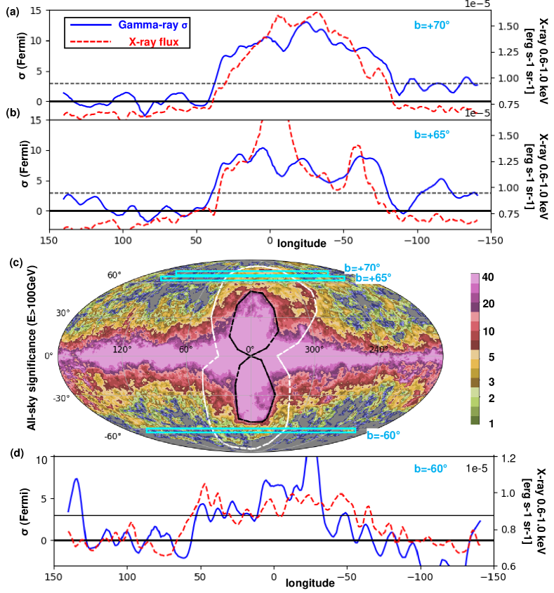
Figure 8: Extended Data Figure 8 $\mid$ Comparison between the X-ray surface brightness (0.6-1.0 keV) and gamma-ray intensity ($E_{\gamma}\gtrsim 100$ GeV) of the eROSITA Bubbles at high Galactic latitudes. Two cuts in the Galactic north (a: $l=+70^{\circ}$, b: $l=+65^{\circ}$) and one cut in the Galactic south (d: $l=-60^{\circ}$) are considered for X-ray (red dashed lines) and gamma-ray (blue lines). Lower latitudes are not considered to avoid the influence from the foreground structures or the Fermi Bubbles. The two energy bands have shown enhancements beyond the background within the edges of the eROSITA Bubbles, and the edges of the enhancements are in agreement with an error of only a few degrees. The consistencies are observed in the southern cut, but the enhanced plateau is less evident for the southern Bubble.

The fact that synchrotron radiation is enhanced at the edges of the eROSITA Bubbles indicates the presence of relativistic electrons. Those electrons can also give rise to gamma-ray emission via inverse Compton (IC) scattering of photons from interstellar radiation and the Cosmic Microwave Background (CMB). We investigate the potential gamma-ray counterparts of the eROSITA Bubbles using the Fermi-LAT data of the diffuse all-sky gamma-ray intensity from [Ref.[23]]. The relative excess of the gamma-ray intensity above the background is presented in Figure 2(a) and Extended Data Figure 6. The horizontal cuts at north and south high Galactic latitudes above and below the Fermi Bubbles are shown in Extended Data Figure 8. We observe that extended structures with $\gamma-$ray enhancements show agreement with a large part of the edges of the eROSITA Bubbles. The consistency in the north can be observed in all three energy ranges for the eROSITA Bubble at mid/high latitude ($b>30^{\circ}$). The consistency in the south is observed for $E_{\gamma}\gtrsim 100$ GeV and for $b\gtrsim-60^{\circ}$ (Extended Data Figure 8), while no clear structure is observed at the cap of the southern eROSITA Bubble. The similarity in the morphology between radio and $\gamma$-ray bands implies a common origin of the emissions in these two bands and we will study their spectral energy distribution.

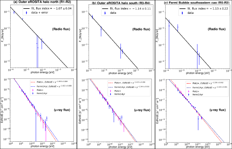
Figure 7: Extended Data Figure 7 $\mid$ Power-law fits for observed fluxes in radio and $\gamma-$ray bands. Upper plots fit the radio fluxes with respect to the energy $F_{\nu}\propto E_{\gamma}^{\alpha_{r}}$. Lower plots fit the gamma-ray fluxes with respect to the energy for Platz+[23] –$EdN/dE\propto E_{\gamma}^{\alpha_{Platz}}$, Fermi14yr – $EdN/dE\propto E_{\gamma}^{\alpha_{F14}}$. (a) northeastern outer outflows (R1-R2). $\alpha_{r}=-1.07\pm 0.04$, $\alpha_{Pl}=-1.499\pm 0.004$, and $\alpha_{F14}=-1.422\pm 0.008$. (b) southeastern outer outflows (R3-R4). $\alpha_{r}=-1.14\pm 0.11$, $\alpha_{Pl}=-1.415\pm 0.006$, and $\alpha_{F14}=-1.344\pm 0.010$. (c) southeastern Fermi Bubble cap (R5-R3). $\alpha_{r}=-1.13\pm 0.22$, $\alpha_{Pl}=-1.239\pm 0.002$, and $\alpha_{F14}=-1.144\pm 0.001$.

We define the region outside the Fermi Bubbles but inside the edges of the eROSITA Bubbles as the outer region. In Figure 2, two patches within the outer region are selected for further investigation: patch R1 in the north ($20^{\circ}<l<40^{\circ}$, $45^{\circ}<b<60^{\circ}$) and patch R3 in the south ($20^{\circ}<l<40^{\circ}$, $-45^{\circ}<b<-30^{\circ}$). The average flux densities in comparison patches outside the eROSITA Bubbles at the same Galactic latitudes (patches R2 and R4, respectively) are subtracted from the two selected patches within the outer region to exclude the influence of foreground emission from the Galactic disc. The radio data[28, 29, 30, 31, 32] from 0.408–30 GHz are used to characterize the synchrotron emission. The effective area of Fermi-LAT drops quickly with decreasing energy below 1 GeV, leading to poor statistics for diffuse emissions in the chosen patches[33]. Therefore, we use only the data beyond 1 GeV in our study. We fit the spectrum with a single power-law in each individual band (radio or gamma-ray, see Extended Data Figure 7), and note that the gamma-ray flux density exhibits a softer spectrum compared to the radio flux in the outer region due to the Klein-Nishina effect.

Assuming the same electrons within a given patch are responsible for both the synchrotron emission and IC scattering, we fit the multi-wavelength SED in different patches of the eROSITA Bubbles to study the cosmic rays (CRs) and magnetic fields therein (Methods). The best-fit results of the SED fitting are presented in Figure 2(c-e). The SED fitting results demonstrate a north/south symmetry of the outer region of the eROSITA Bubbles. The derived electron distributions $N\propto E^{\alpha}$ have shown consistent, very steep slopes, with $\alpha=-3.40\pm 0.06$ in the northern patch R1 and $-3.38\pm 0.10$ in the southern patch R3. The magnetic field directions are largely symmetric about the Galactic disk, and the average magnetic field strengths are $1.97\pm 0.20$ $\mu$G in the north and $1.40\pm 0.20$ $\mu$G in the south. Adopting a temperature of 0.3 keV[8], a halo electron density of $3\times 10^{-3}$ cm^-3 calculated from [Ref.[34]], and magnetic field strength obtained through our SED fitting, we calculate the plasma beta in patch R1: $\beta_{r1}\simeq 9$, and in patch R3: $\beta_{r3}\simeq 18$.

Plausible origins of the CRs responsible for the non-thermal radiation in the outer region of the eROSITA Bubbles include acceleration processes in the inner Fermi Bubbles or Galactic outflows from the disc. As a comparison, we perform an SED fitting for the southeastern edge of the Fermi Bubbles in Figure 2(e) and find an electron energy index $-3.00^{+0.3}_{-0.13}$ for patch R5. This electron index is harder than that in the patch R3 of the outer region at the same latitude. We compare the synchrotron flux densities for the outer patch R3 and the inner patch R5 after foreground subtraction, for 0.408 GHz: $F_{\nu,R3}=0.0523\pm 0.0078$ MJy/sr, $F_{\nu,R5}=0.0140\pm 0.0099$ MJy/sr; for 1.4 GHz: $F_{\nu,R3}=0.0082\pm 0.052$ MJy/sr, $F_{\nu,R5}=0.0118\pm 0.0059$ MJy/sr; for 23 GHz: $F_{\nu,R3}=(5.9\pm 4.6)\times 10^{-4}$ MJy/sr, $F_{\nu,R5}=(3.4\pm 6.7)\times 10^{-4}$ MJy/sr; for 30 GHz: $F_{\nu,R3}=(3.3\pm 1.3)\times 10^{-4}$ MJy/sr, $F_{\nu,R5}=(1.5\pm 1.4)\times 10^{-4}$ MJy/sr. The synchrotron flux densities in the outer region are equvalent or higher compared to the foreground-subtracted values inside the Fermi Bubbles at a similar Galactic height. Therefore, diffusion from the Fermi Bubbles cannot be the primary process for injecting the relativistic electrons into the outer region. Additionally, the magnetic field is parallel to the shell of the Bubbles and the diffusion from the Fermi Bubbles into the outer halo requires the cross field transport of relativistic electrons, which is very inefficient.

Figure 3 shows that magnetic ridges of the outer region connect to the locations having high star-formation rates in the disc, corresponding to the star-forming ring of our Galaxy. The magnetised ridges related to the Fermi Bubbles, on the other hand, appear to originate from the few-hundred parsec Central Molecular Zone (CMZ) and to wrap around the surface of the Fermi Bubbles, which is consistent with previous works[6, 35]. This distinction is also consistent with the conclusion above that there are different origins of relativistic electrons in the Fermi Bubbles and the outer region. In search of the sources for relativistic electrons, we show in Figure 3c a polar view of the specific star-formation rate distribution in the Milky Way, as measured by Herschel[36], displaying several clumps in the star-forming ring with rates $\Sigma_{SFR}\gtrsim 0.02~{}\mathrm{M_{\odot}yr^{-1}kpc^{-2}}$. This distribution aligns with the footprint of the magnetised ridges, which gives us a clue to the origin of these relativistic electrons in the outer region. The collective effect of merging supernova explosions can generate a Galactic wind by expelling material at speeds ranging from $100$ to $1000$ km s^-1 out of the Galactic disc[37, 38, 39, 40]. Consequently, a wind termination shock is anticipated at far end of the wind, where particles are accelerated and heated. Hence, the primary source of CRs responsible for the outer region is likely to be the Galactic outflows from the star-forming ring (hereafter “outer outflows”). The radio-gamma flux densities in the outer outflows can be effectively modeled by electrons with energies higher than 2 GeV, following a single power-law distribution. This supports the hypothesis of a shared origin for the multi-wavelength radiations. The electron index of $\alpha\simeq-3.4$ observed in the outer outflows is too soft with respect to the expectation from the strong shock acceleration (the classical value for the index of the strong shock is $\alpha=-2$)[41, 42]. Instead, the observed soft spectrum arises from a significant cooling above 2 GeV within the investigated patches. This indicates that the dynamic timescale of the outer outflows is longer than the cooling timescale of the relativistic electrons, $10^{8}$ yr (see Methods). In this scenario, the thermal X-ray emission of the eROSITA Bubbles comes from the shock-heated plasma. Applying the Rankine-Hugoniot relation, we find that the wind velocity is approximately $v_{w}\sim 400$ km/s (Methods), falling within the anticipated range for galactic winds driven by collective supernova explosions. Our calculations indicate that sustaining the outer outflows requires less than $15\%$ of the energy released from supernova explosions in the star-forming ring and the mass loss rate from the star forming ring would be 0.3-0.9 M_⊙/yr (see calculations in Methods and Extended Data Table 2).

We present a detailed 3D picture for the eROSITA Bubbles in Figure 3d, where the outflows form a “bouquet” shape in the Galactic halo. In our model, magnetic ridges appear as coherent structures emerging from the active star-forming regions in the Galactic disc. Early researches[43, 6, 44] found that Galactic halo medium rotate clockwise as seen from the Galactic north, similarly to the disc medium, and the azimuth rotation speed decreases with the height from the disc. External spiral galaxies show a similar behavior and have been found to have a lag in the halo with a reduction of the gas rotational speed on the order of $10~{}\mathrm{km/s}\,\frac{H}{~{}\mathrm{kpc}}$[45, 46], where $H$ is the height from the Galactic plane. Figure 3e shows that the angular lag of the field lines with increasing height from the Galactic plane can explain the general orientation of the magnetic field, aligned with the ridges in the east edges and westwards oriented in the west. Recent simulations[47] of the magnetic halo of galaxies found that ordered magnetic fields are associated with free gas winds. Thus, the magnetic ridges trace the outflows that have a slower angular speed at increasing heights. This is consistent with what was previously found for the magnetic ridges wrapping the Fermi Bubbles[6], thus suggesting similar gas dynamics for the inner and outer outflows.

Our results show there is a connection between the X-ray-emitting and magnetised Galactic halos and offer insights into the origin of these halos in other galaxies. We show that star-forming activities play an important role in the formation of these halos. Notably, observations of edge-on galaxies have revealed a distinctive X-shaped magnetic halo at radio frequencies, featuring kpc-scale anisotropic magnetic ridges emerging from the galaxy’s inner region[2]. Such features can be attributed to galactic outflows launched from active star-forming regions, which can regulate the gas ecosystem of galaxies and have a fundamental impact on the galactic evolution.

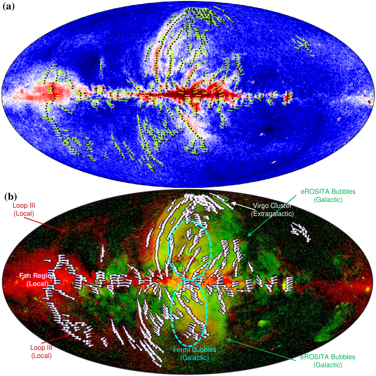
Figure 1: Figure 1 $\mid$ Polarized radio counterpart of the eROSITA Bubbles. (a) Background image: polarized synchrotron intensity (PI_syn) from WMAP data at 22.8 GHz; Black dots: local maxima of the polarized synchrotron intensity estimated from constant latitude profiles; Green bars: magnetic field direction inferred from polarized synchrotron emission. Several coherent magnetised ridges rise from the Galactic disc and are progressively bent toward the west with increasing latitude. (b) Magnetised ridges (PI_syn,max, white dots) and polarized synchrotron emission at 22.8 GHz (red) compared to the eROSITA X-ray emission at 0.6-1.0 keV (green). The large structure close to the east end of the map with no X-ray counterpart is the Fan Region (local emission, see Extended Data Figure 5). The magnetised ridges in the inner Galaxy ($\mid l\mid\lesssim 60^{\circ}$) are spatially correlated with Galactic structures: the ridges associated spatially with the Fermi Bubbles appear to emanate from the CMZ[6, 26, 27], while the ridges in the outer region appear to originate in the disc a few kpc from the Galactic Centre. The ridges show an approximate north-south symmetry. The polarized intensity is enhanced at the edges of the eROSITA Bubbles. The eastern edges of these Bubbles are parallel to their magnetic field. The western roots of the eROSITA Bubbles’ edges are limb-brightened in polarized synchrotron emission.

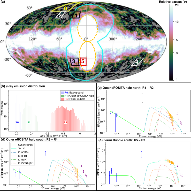
Figure 2: Figure 2 $\mid$ Radio–$\gamma$-ray analysis and SED. (a) Intensity map (defined in Methods) of the Fermi all-sky diffuse map at $E_{\gamma}\gtrsim 100$ GeV expressed in units of the noise level from the reference background (patch R0 in the northeastern high galactic latitude sector). Patches R1-R5 are used for the SED study. The two solid lines are the edges of the eROSITA and Fermi Bubbles. (b) the distribution of the pixel counts for the gamma-ray fluxes in the background (R0), the outer region of the eROSITA Bubbles (R1), and the Fermi Bubble (R5). The three distributions are well separated. (c-e) SED best-fit of leptonic radiation in: (c) the outer region north (R1-R2) with electron energy index $-3.40\pm 0.06$ and magnetic field $1.97\pm 0.20$ $\mu$G; (d) south (R3-R4) with electron index $-3.38\pm 0.10$, magnetic field $1.40\pm 0.20$ $\mu$G; (e) southeastern cap of the Fermi Bubble (R5-R3) with electron index $-3.00^{+0.30}_{-0.13}$, magnetic field $1.0^{+0.5}_{-0.4}$ $\mu$G. The fitting results for the electron distribution indices for the outer regions are consistent, but the Fermi Bubble has a harder electron energy distribution index. The detailed results are summarized in Extended Data Table 1.

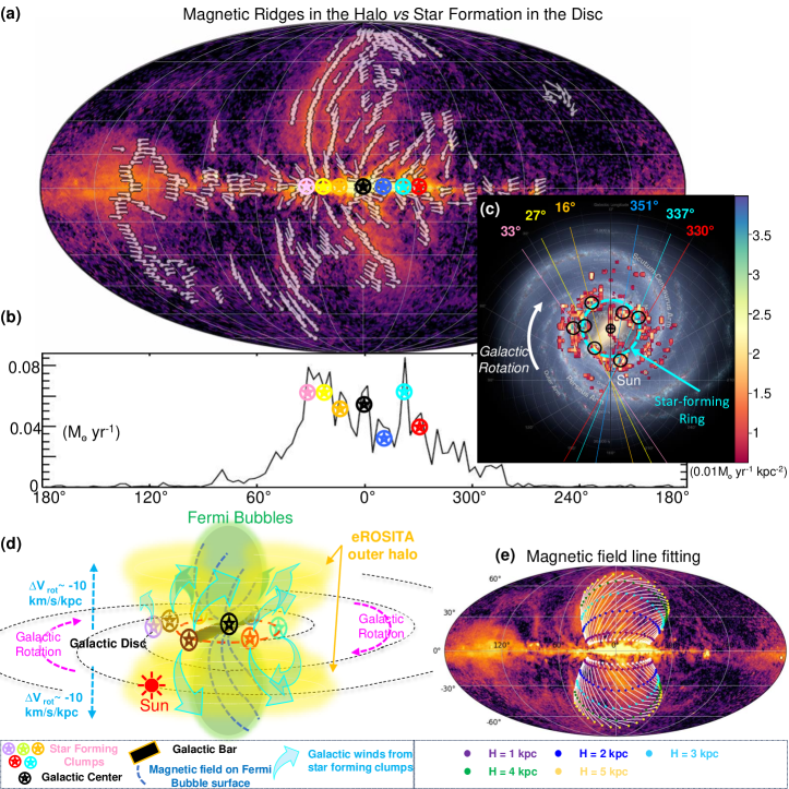
Figure 3: Figure 3 $\mid$ Energy sources of the Galactic outflows. (a) the polarized intensity map with at 22.8 GHz by WMAP the magnetic ridges (white bars) overlaid. The footpoints of the magnetic ridges correspond to the marked clumps with a high star-formation rate on the Galactic plane in (b). (c): an artistic view of the Galaxy (NASA/JPL-Caltech/R. Hurt) with the active star-forming clumps and their Galactic longitude overlaid. The specific star formation rates are measured from [Ref.[36]] binned by a resolution of $0.5\times 0.5~{}\mathrm{kpc^{2}}$, and the clumps with $\Sigma_{SFR}\gtrsim 0.02~{}\mathrm{M_{\odot}yr^{-1}kpc^{-2}/bin}$ are considered. (d) Proposed scenario for the observed multi-wavelength Milky Way outflows. The star-forming ring powers the outer outflows, showing a “bouquet” morphology. We assume the presence of a central outflow that generates the Fermi Bubbles, as discussed in previous works[35, 26]. We note that some magnetised ridges appear to be wrapped around the Fermi Bubbles. The outflows show a lag as the plasma is transported to higher Galactic latitudes because of the decrease of rotational speed at higher heights from the plane. (e) Modelling of the field line flow wrapping around the surface of the outer outflows. An angular lag of $4.5^{\circ}\frac{\mathrm{H}}{\mathrm{kpc}}$ with an increasing height H is used. The east-to-west tilted orientation of the magnetic ridges can be reproduced by such lagging. The resulting magnetic field is parallel to the surface of the Bubbles, providing confinement to the CRs.

Methods

Multi-wavelength data

We use the following surveys in our paper to analyze the magnetic halo: the polarized synchrotron emission surveys at different frequencies – Haslam408 (0.408 GHz)[48, 49, 28]; DRAO/Villa-Elisa (1.4 GHz)[29, 50], S-PASS (2.3GHz)[6, 51], QUIJOTE (11, 13 GHz)[30], WMAP K-Band (22.8 GHz)[15, 52], and Planck (30 GHz)[53]. To exclude the local contribution we use the dust polarized emission at 353 GHz from Planck [54]. The SED analysis made use of the diffuse $\gamma-$ray emission measured by Fermi-LAT (1 GeV to 200 GeV) with sources subtracted off[23]. The diffuse Fermi emission is compared with data from Fermi 14 year data subtracting the 14-year Fermi point source catalog[55]. The HAWC[56] also provides constraints to the SED. The Gaia-2MASS survey uses the star dust absorption of the Gaia survey to study the dust structures at different distances[19]. The X-ray emission the energy band 0.6–1.0 keV by eROSITA was used [8] for the eROSITA Bubbles. The data of the energy band 0.11–0.28 keV are from ROSAT[57]. The star-forming rates of the Galactic disc are from the infrared Herschel Legacy survey[36]. For processing and analyzing the observational data, we use Python[58] with the package Numpy[59, 60], Healpy[61, 62], Astropy[63, 64, 65], Fermipy[66]; Jupyter Notebook[67], Matplotlib[68]; and DS9[69].

Distance measurements through X-ray and dust observations

We estimate the distance to the X-ray emitting eROSITA Bubbles in Extended Data Figure 3. The X-ray photons emitted by hot plasma can be absorbed by foreground medium. Extended Data Figure 1(c) shows that an anti-correlation is observed between the eROSITA Bubbles (0.6–1.0 keV) and the contour of polarized intensity from the dust at $\mathrm{PI_{dust}}=22\mu$K. On the other hand, Extended Data Figure 3(d) reports the anti-correlation between softer X-ray emission from ROSAT[57] (0.11–0.28 keV) and the contour of a lower polarized intensity from the dust ( $\mathrm{PI_{dust}}=5\mu$K). We take the measurements from [Ref.[19]], and integrate the extinction for distances lower than $500$ pc around the Sun, as obtained from the 3D dust distribution by the Gaia-2MASS-Apogee dataset. Extended Data Figure 3(b) shows that the polarized dust intensity from Planck survey is originated mainly from the local medium. The X-ray absorber for softer X-ray emission has extended to a higher Galactic latitude. This is consistent with the picture that the bulk of the X-ray emitting structure is behind the dust within 500 pc. Therefore we conclude that the eROSITA Bubbles stand behind the dust emission within 500 pc from the Sun, beyond the Local Arm. Hence, they should extend above and below the Galactic disc. The distance to magnetic ridges will be estimated in the Faradaty-Rotation depolarization analysis in later paragraphs.

Comparison between dust and synchrotron polarization

We obtain the magnetic ridges by performing same-latitude cuts across the all-sky polarized synchrotron emission map (PI_syn) from WMAP K band[15] to find the local maximum points (PI_syn,max) along each cut. The points with PI${}_{syn,max}>0.04$ K are preserved in Figure 1, and the corresponding magnetic field directions are overlaid. Several coherent magnetic structures extending more than $15^{\circ}$ are found and we define them as magnetic ridges. Extended Data Figure 3(b) demonstrates that the polarized dust intensity from Planck survey are originated mainly from the thermal dust within 500 pc from us. Simulations of dust emission at 353 GHz also show that it is consistent with dust emission of the Local Bubble[70] that is within 200 pc from the Sun[71, 72]. Extended Data Figure 1 presents the comparison between polarization angles of dust (353 GHz) and synchrotron polarized emission. The polarization angle of the synchrotron emission is perpendicular to the direction of the magnetic field (on the plane of the sky), whereas the dust polarization angle at mm-wavelengths is perpendicular to the magnetic field. As shown in Extended Data Figure 1(b), the known local structures, the Fan Region, and most of the Galactic plane ($\mid b\mid<5^{\circ}$) apply to the dust polarization parallel to the magnetic field. There is no uniform correlation between the magnetic field and dust polarization in the Serpens-Aquila Rift. Furthermore, most of the magnetic ridges corresponding to the outer region of the eROSITA Bubbles and the southern Fermi Bubbles have no dust counterparts. Hence these ridges are Galactic structures which are not contaminated with other components along the line-of-sight. Because the polarized synchrotron emission also does not have the distance information for the emitting layer, we will introduce the Faraday rotation depolarization analysis below to measure the distances to those magnetic ridges.

Faraday rotation depolarization analysis

The depolarization is the ratio between the polarization fraction at a frequency and that at a reference frequency, assumed not depolarized. The polarized intensity and polarization angles of the magnetic ridges show wavelength-dependent depolarization. Based on the derivations from [Refs.[20, 22, 73]], the wavelength-dependent Faraday depolarization for a synchrotron-emitting and Faraday rotating turbulent magneto-ionic plasma is:

$$f_{depol}=\frac{1-\exp(-S)}{S},$$ (1)

where $S\equiv 2\sigma_{RM}^{2}\lambda^{4}$. In our calculations, we pick the $22.8$ GHz of the WMAP[74] data as the reference frequency, at which the Faraday rotation depolarization can be assumed negligible. The RM dispersion $\sigma_{\rm RM}$ is:

$$\sigma_{RM}=0.81\,\sigma_{B\parallel}\,n_{e}\,d\,N_{\mid\mid}^{1/2}$$ (2)

where $n_{e}$ [cm^-3] is the electron number density of the plasma, $\sigma_{B\parallel}$ [$\mu$G] is the component along the line.-of-sight of the isotropic, turbulent magnetic field, and $N_{\mid\mid}$ is the number of random-walk cells of length $d$ [pc] along the line-of-sight. The latter is defined as $N_{\mid\mid}\equiv L\,f/d$ where $L$ [pc] is the distance from us and $f\equiv<n_{e}>^{2}/<n_{e}^{2}>$ is the electron volume filling factor. The RM dispersion can thus be written as[75]:

$$\sigma_{RM}^{2}=\left(0.81\,\sigma_{B\parallel}\right)^{2}\,L\,d\,<n_{e}^{2}>$$ (3)

The cell length is assumed[76, 77, 73] $d=100~{}\mathrm{pc}$. We use the electron density model by [Ref.[78]] and the turbulent magnetic field of the model by [Ref.[79]] modified to fit Planck results[80]. We assume a distance of the Sun from the Galactic Centre of $D_{\odot}=8.5~{}\mathrm{kpc}$. Given a position on the line-of-sight of Galactic coordinates ($l$, $b$) and a distance $L$ from the Sun, the position in the Galaxy can be expressed as:

$$\begin{array}[]{ll}r&=\sqrt{D_{\odot}^{2}+L^{2}\cos^{2}(b)-2D_{\odot}L\cos(b)\cos(l)},\\ z&=L\sin(b),\\ \end{array}$$ (4)

where $r$ is the separation from the Galactic Centre on the Galactic plane and $z$ is the height from the plane. Along each line of sight, we perform the integration with a discrete step ${\delta L}=5~{}\mathrm{pc}$, which yields an RM dispersion of:

$$\begin{split}\sigma_{RM}^{2}&=\int_{L}^{O}\left(0.81\,B_{\parallel}(l,b,L)\right)^{2}\,d\,n_{e}^{2}(l,b,L){\bf\delta L}\\ &=\int_{L}^{O}\left(0.81\,\frac{B_{JF12}(l,b,L)}{\sqrt{3}}\right)^{2}\,d\,n_{e}^{2}(l,b,L){\bf\delta L}\\ \end{split}$$ (5)

where $B_{JF12}$ is the magnetic field strength adopted from [Refs.[79, 80]], and the factor $1/\sqrt{3}$ represents the line-of-sight component. Additionally, the wavelength-dependent dispersion caused by the foreground medium with $\sigma_{\rm RM}$ is:

$$\Delta\Phi=\sigma_{RM}\lambda^{2}$$ (6)

The results from these equations are shown in Extended Data Figure 3, panels e-g, and in Extended Data Figures 4 and 5. We estimate the depolarization from the observations at three different frequencies (22.8, 2.3, and 1.4 GHz using data from WMAP[15, 52], S-PASS[6, 81], and DRAO/Villa-Elisa surveys[29, 50], respectively). The depolarization gets smaller moving to high latitudes and higher frequencies. The depolarization screen generated by the magneto-ionic medium out to 5-kpc is reported in Extended Data Figure 4. Our calculations tells that the depolarization depends on the frequency and the latitude that determines how much of the disc the polarized radiation goes through. Specifically: in Zone A (high latitudes $\mid b\mid\gtrsim 20^{\circ}$), both 1.4 and 2.3 GHz can be observed; in Zone B (mid latitudes $5^{\circ}\lesssim\mid b\mid\lesssim 20^{\circ}$), 1.4 GHz is depolarized whilst 2.3 GHz is observable ; in Zone C (low-latitudes $\mid b\mid\lesssim 5^{\circ}$) both 1.4 GHz and 2.3 GHz are depolarized. Negligible depolarization occurs at 22.8 GHz at any latitudes and the magnetic coherence are preserved from the Galactic disc up to the Galactic poles. Extended Data Figure 3, panel g, shows the observed polarized emission at 1.4 GHz (DRAO/Villa-Elisa)[29, 50], 2.3 GHz (S-PASS)[6, 81], and at 22.8 GHz (WMAP)[15, 52]. The image also shows that our calculations of the depolarization broadly match the regions of high depolarization. Our analysis indicates that the polarized emission from the magnetised ridges in the inner Galaxy must originate from the medium situated beyond several kpc from us. Extended Data Figure 5 shows the regions with high polarization intensity at 1.4 GHz at low Galactic latitudes (i.e., the Fan Region and Loop III). These regions can be interpreted as local, or at a distance closer than some 1-kpc. This is consistent with previous measurements at $150$ MHz[82]. Instead, the Galactic magnetised ridges coincident to the eROSITA Bubbles are clearly depolarized at 1.4-GHz at low and mid Galactic latitudes, consistently with the prediction of a depolarization screen at a distance of at least 5 kpc. The frequency sensitive depolarization does not affect the local structures.

Diffuse $\gamma-$ray Fermi radiation

In our $\gamma-$ray intensity map, we calculate the relative excess of the $\gamma-$ray flux along different lines-of-sight comparing to the standard deviation of the selected background area located at high Galactic latitude towards the northeast (patch R0 in Figure 2a). The relative excess is defined by $\sigma\equiv(I_{f}-\overline{I}_{f0})/std(I_{f0})$, where $I_{f}$ is the flux at a given line-of-sight, $\overline{I}_{f0}$ and $std(I_{f0})$ are the average value and standard deviation of the background patch. The results are presented in Figure 2a and Extended Data Figure 6.

Consistency of the X-ray eROSITA Bubbles’ edges with other wavelengths emission

We compare the magnetised ridges, as we defined them using synchrotron polarization data from WMAP[15, 52], with the X-ray surface brightness at 0.6-1.0 keV in Extended Data Figure 2. The polarized intensity is enhanced at the edges of the eROSITA Bubbles, with the only exception of the south-west Bubble’s edge. The enhancements of the PI_syn at all of the four roots of the eROSITA Bubbles suggests that the eROSITA Bubbles are limb-brightened in synchrotron polarized emission, similarly to the roots of the Fermi Bubbles[35, 6]. The magnetic field directions are parallel to the eastern edges of the eROSITA Bubbles in both the north and the south. Instead, there is no alignment in the west, where the field is tilted westwards. A possible explanation is given by the modelling presented in the main text and Figure 3(e). The points at the same height ($H=1\sim 5$ kpc) on the eROSITA Bubbles’s surface are projected on the polarized synchrotron intensity map. An anticlockwise lag of $4.5^{\circ}$ is introduced between points differing in height by $\Delta H=1$ kpc. The global east-to-west tilt is reproduced in the fitting and the field direction is tilted westward compared to the ridges orientation, consistently with what observed.

The comparison between X-ray and $\gamma-$ray for eROSITA Bubbles is performed in Extended Data Figure 8. We perform cuts in high Galactic latitudes in the north ($b=+70^{\circ}$ and $+65^{\circ}$) and south ($b=-60^{\circ}$) to avoid the potential influence by the emission from the foreground Galactic disc or the Fermi Bubbles. In the northern cuts, both X-ray and $\gamma-$ray radiations have shown central enhancements ($-70^{\circ}\lesssim l\lesssim 40^{\circ}$) beyond the background within the edges of the eROSITA Bubbles with a clear “plateau” shape. Additionally, the edges of the enhancements are in agreement with an error of only a few degrees. In the southern cut, the central enhancements are observed for both X-ray and $\gamma-$ray bands, but they are less evident as compared to the cuts in the Galactic north. Below $b=-60^{\circ}$, there is no clear edge of $\gamma-$ray emitting structures.

SED data and fitting consideration

The spectral energy is computed as $E^{2}d^{4}N/(dEdAd\Omega dt)$. For $\gamma-$ray, the data is: the energy of the photons received at the receiver (area A) at a given band width (log-spaced) per solid angle per time (using the notation E²dN/dE for simplicity).

For radio data, spectral flux density ($\mathcal{F}(\nu)$) is the quantity that describes the rate at which energy is transferred by electromagnetic radiation through a surface, per unit surface area and per unit frequency. $\mathcal{F}(\nu)=\frac{\partial F}{\partial\nu}$, where F is the flux density. The SED quantifies the energy emitted by a radiation source in the log energy band, hence (in the unit of  erg s^-1 cm^-2 sr^-1):

$$\begin{array}[]{ll}\nu\mathcal{F}(\nu)&=\nu\frac{\partial F}{\partial\nu}=\frac{\partial F}{\partial(\log(\nu))}\\ &=\frac{S[{\rm MJy/sr}]}{10^{17}{\rm MJy}/[{\rm erg\cdot s^{-1}\cdot cm^{-2}\cdot Hz^{-1}]}}*\nu[{\rm Hz}]\\ \end{array}$$ (7)

For the $\gamma-$ray flux density, we use the diffuse emission from Fermi-LAT with energy higher than 1 GeV, and we use the HAWC sensitivity as upper limits for $E_{\gamma}\gtrsim 1$ TeV as the Bubbles are not observed by HAWC[56]. We use two methodologies to extract the diffuse gamma-ray emission of the give patches:

1) We use the diffuse radiation after the point sources subtraction from Platz+[23] using a Bayesian analysis on the 12 year Fermi data (hereafter Platz+). Platz+ separates the data in the range $0.316$ GeV$\lesssim E_{\gamma}\lesssim 316$ GeV into 11 energy bins. In order to compute data uncertainties, we consider: (1a) The standard deviation of the flux intensity among all pixels in the patch ($n_{st}=std(I_{R})$); (1b) The Poisson noise of the observed photons ($n_{pois}=\frac{\sqrt{N}}{N}\bar{I}_{R}$, where N is the total number of photons and $\bar{I}_{R}$ is the average flux intensity in the patch). Hence, the total error of the patch is defined by $err_{R}=\sqrt{n_{st}^{2}+n_{pois}^{2}}$. We then use the normal error propagation rules in order to compute the uncertainty of the $gamma-$ray maps. Take patch R1 subtracted by patch R2 as an example:

$$\begin{array}[]{ll}Signal:&I_{signal}=I_{R1}-I_{R2}\\ Noise:&s_{noise}=\sqrt{(err_{R1})^{2}+(err_{R2})^{2}}\\ \end{array}$$ (8)

where $err_{R1}$ and $err_{R2}$ are the total errors in patch R1 and patch R2.

2) Complementary, we take the diffuse $\gamma-$ray data of the same patches from the 14 year Fermi-LAT data (hereafter Fermi14yr). Fermi14yr uses the most recent Fermi data and the 14 year source catalog 4FGL-DR3 [55]. Fermi14yr separates the data in the range $0.1$ GeV$\lesssim E_{\gamma}\lesssim 500$ GeV into 25 energy bins. We mask the influence from the point sources within a radius of $14^{\circ}$ from the boundaries and find the best fit for the diffuse emission through Fermipy[66]. The outcome indices ($dN/dE\propto E_{\gamma}^{\beta_{F14}}$) for the emission from the 5 patches by a power-law fitting are: patch R1: $-2.180\pm 0.002$; patch R2: $-2.235\pm 0.003$; patch R3: $-2.205\pm 0.002$; patch R4: $-2.167\pm 0.002$; patch R5: $-2.092\pm 0.002$. We can see that these fitting indices are rather similar to each other. Therefore, it is necessary to exclude the Galactic foreground influences in our analyses.

To perform foreground subtraction in our fitting, we remove the average flux outside the bubbles’ edge at the same latitude. In the southeastern sky ($b>30^{\circ},60\lesssim l\lesssim 150^{\circ}$), there are several known local structures which might influence the estimate of the total flux (see Extended Data Figure 1a and 5). Therefore we select the patch R4 in the southwestern sky to represent the foreground. As demonstrated in Figure 2a, we choose the patches in the mid-latitude: R1 and R3 for northern/southern outer region of the eROSITA Bubbles, R5 for southern Fermi Bubble cap (northern Fermi Bubble is not selected because it is overlapped with the Serpens-Aquila Rift, see Extended Data Figure 1b). In order to exclude the influence of the emission of the foreground, we subtract the emission at the same Galactic latitude outside the considered patches (i.e., patch R1-patch R2; patch R3-patch R4; patch R5-patch R3). We plot the flux density of 0.6-1.0 keV at the corresponding patches from [Ref.[8]] in the SED for reference.

Fitting of the photon field for IC Based on our analysis, the patches that we study would be only a few kpc away from the Galactic disc, hence the seed photons in IC radiations of the SED fitting are mainly from the Interstellar radiation field (ISRF) plus the CMB. We neglect the slight anisotropy in the starlight radiation field and only considers the fitting of radiation energy density based on the radiation model proposed by [Ref.[83]] and simplify the seed photon field by fitting the radiation spectrum with 4 blackbody radiation fields at “CMB” (at 2.725 K), “FIR” (far-infrared), “NIR” (near-infrared), “Star-light” (scattered star light from the Spiral Arms of the Galaxy). We present the 4-blackbody modellings in the Supplementary Figure 1-3(a) and summarize the results in Extended Data Table 1(a).

MCMC fitting for SED We use the package “naima”[84] to model the multi-wavelength results. We choose to see if the multi-wavelength emission fits purely leptonic processes (Synchrotron + Inverse Compton). We assume that the synchrotron and Inverse Compton (IC) emissions are from the same electron distributions of the same patches. The synchrotron emission spectrum of the “naima” package is calculated from magnetic field strength and electron distribution based on [Ref.[85]]. The IC emission spectrum of the “naima” package is calculated from seed photon fields and electron distribution based on [Ref.[86]].

We presume the electron distribution to be in a power-law following the equation defined in “naima”:

$$f(E_{e})=A_{e}(\frac{E_{e}}{1~{}\rm TeV})^{\alpha},$$ (9)

where $A_{e}$ [eV^-1] is the amplitude of the electron spectrum, $\alpha$ is the electron index, and $E_{e}$ is the electron index.

The non-detection of the Bubbles from the HAWC survey provides the upper limit in our SED fitting in $E_{\gamma}\gtrsim$1 TeV bands. As a result, the SED data cannot be fitted with a single power-law distribution of electrons. We also test the electron distribution with an exponential cut-off at the high-energy end of the electron spectrum following the equation defined in “naima”:

$$f(E_{e})=A_{e}(\frac{E_{e}}{1~{}{\rm TeV}})^{\alpha}\exp(-(\frac{E_{e}}{E_{\rm cutoff}})^{\beta_{e}}),$$ (10)

where we take $\beta_{e}=2$ as the cut-off power index based on [Ref.[87]].

In our fitting, linear priors are used for all the parameters and the first 500 steps are discarded as the burn-in phase. We run $5\times 10^{3}$ steps to get the best fit and errors of the amplitude $A_{e}$, the index $\alpha$, and the magnetic field strength $B$. These setups are enough to achieve Gaussian distribution for all the tested parameters (see Supplementary Figures 1-3). The fit results are summarized in Extended Data Table1(b).

Fitting results

We first show the power-law fit for the fluxes of individual energy bands in Extended Data Figure 7: the radio flux ($F_{\nu}\propto E_{\gamma}^{\alpha_{r}}$), and the gamma-ray flux ($EdN/dE\propto E_{\gamma}^{\alpha_{Pl}}$ for Platz+[23] and $EdN/dE\propto E_{\gamma}^{\alpha_{F14}}$ for Fermi 14 year diffuse map[55]).

The gamma-ray spectral indices obtained from the two tested-methods have small differences ($\Delta\alpha_{\gamma}\lesssim 0.1$, e.g., for northeastern outer halo, $\alpha_{Pl}=-1.499\pm 0.004$, and $\alpha_{F14}=-1.422\pm 0.008$). They are consistent with each other considering the systematic uncertainties of the Fermi-LAT[88]. For reference, the power-law index obtained in the southeastern cap of the Fermi Bubbles at the same latitude is significantly harder ($\alpha_{Pl}=-1.239\pm 0.002$).

The radio fluxes in the outer halo show a harder spectrum compared to the gamma-ray flux for the outer outflows (for northeastern outer halo: $\alpha_{r}=-1.07\pm 0.04$, $\alpha_{Pl}=-1.499\pm 0.004$; for southeastern outer halo: $\alpha_{r}=-1.14\pm 0.11$, $\alpha_{Pl}=-1.415\pm 0.006$). But we need to note that the $\gamma-$ray emissions are influenced by the Klein-Nishina (KN) effect at higher energy which would result in a softer spectrum. Therefore we need to check if the radio and $\gamma-$ray flux densities could be fitted with one single power-law electron distribution in the SED fitting. As is shown in the Extended Data Table 1(b), the SED fitted magnetic field strength and electron indices based on Platz+[23] and Fermi14yr[55] are consistent for all the fittings within error range.

The MCMC processes and corner maps, are presented in Supplementary. Especially, Supplementary Figure 1-3(b) show that the multi-wavelength data dispersion is within 2-$\sigma$ to the best fit and the Gaussian distribution for all the parameters have been reached.

We can verify the obtained magnetic field based on the SED fitting as follows: The typical IC photon energy radiated by an electron with the energy $E_{e}$ up-scattering a photon of energy $\epsilon\,$ can be given by $E_{\rm IC}\approx 3(E_{e}/40\,{\rm GeV})^{2}(\epsilon/0.4\rm eV)\,$GeV, given that the KN effect is not important. The same electron radiates synchrotron photon in the magnetic field $B$ at a typical energy of $E_{\rm syn}=10^{-4}(E_{e}/40{\rm GeV})^{2}(B/1\mu\rm G)\,$eV. Combing this two formulae, we get

$$E_{\rm IC}\approx 3(E_{\rm syn}/10^{-4}{\rm eV})(B/1\mu\rm G)^{-1}(\epsilon/0.4\rm eV)\,{\rm GeV}.$$ (11)

On the other hand, the synchrotron-to-IC flux ratio is $F_{\rm syn}/F_{\rm IC}=u_{\rm B}/u_{\rm ph}$. Take the north outer outflow for instance, the $\gamma$-ray flux at 3 GeV is measured to be about $10^{-9}\,\rm erg~{}s^{-1}cm^{-2}sr^{-1}$, and the radio flux at $10^{-4}\,$eV is about $4\times 10^{-10}\,\rm erg~{}s^{-1}cm^{-2}sr^{-1}$. For a soft electron spectrum, the optical radiation field is the dominant target radiation field for the IC radiation at 3 GeV, at which energy the KN effect is not important. Thus, for $u_{\rm ph}=0.23\,{\rm eV/cm^{3}}$ and $\epsilon\approx 0.4\,$eV, we obtain $B\approx 1.9\,\mu$G via Eq. (11), which is consistent with the fitting result.

We calculate the cooling time for the non-thermal radiations from the electron at the energy $E_{e}$ [Ref.[89]] based on the following equation considering the synchrotron cooling time $\tau_{syn}$ and the Inverse Compton cooling time $\tau_{IC}$:

$$\begin{array}[]{ll}\tau_{cool}&=(\tau_{syn}^{-1}+\tau_{IC}^{-1})^{-1}\\ &\simeq 5\times 10^{8}\left(\frac{E_{e}}{1~{}\mathrm{GeV}}\right)^{-1}\left(\frac{U_{B}+U_{\rm ph}}{10^{-12}~{}\mathrm{erg}~{}\mathrm{cm^{-3}}}\right)^{-1}~{}\mathrm{yrs}\\ \end{array}$$ (12)

where $U_{B}\equiv\frac{B^{2}}{8\pi}$ is the magnetic energy and $U_{ph}$ is the energy density for the radiation field relevant to the IC process. The relativistic Bremsstahlung is negligible in our analysis because the gas density in the halo is too low and the corresponding cooling time is more than $10$ Gyr.

Outer outflow modelling

Regions with a star formation rate surface density larger than 0.01 $\mathrm{M_{\odot}yr^{-1}kpc^{-2}}$ drive superwinds that can become galaxy outflows of speed of $\sim$ 100–1000 km/s[37, 38, 40, 90]. Figure 3c shows the star-formation rate density of the Milky Way’s disc as measured with Herschel telescope data[36]. We find that there are several clumps that have sufficient star formation rate to drive galactic winds and that are at and about the star-forming ring located at 3-5 kpc from the Galactic Center.

The energy injection rate in the outer halo can be estimated by:

$$E_{tot}\sim\dot{E}_{inj}\min\{t_{dyn},t_{therm,cool}\}$$ (13)

where $E_{tot}$ is the total energy in the outer halo, $t_{dyn}$ is the dynamical timescale of the outer halo and $t_{therm,cool}$ is the cooling time of the hot plasma. The quantity $\dot{E}_{inj}$ is the energy injection rate into the system. The system energy depends on the system time before the cooling is dominant, whilst it depends on the cooling time when it is shorter than age of the outer halo ($t_{dyn}>t_{therm,cool}$). The cooling time for the hot plasma in the eROSITA Bubbles is estimated of approximately $2\times 10^{8}$yrs [8].

The total energy injection is made up of 1) the thermal energy of the hot plasma ($\dot{E}_{therm}$), 2) the energy of non-thermal electrons ($\dot{E}_{CR}$), and 3) the magnetic field energy ($\dot{E}_{B}$). The energy in the hot thermal plasma that emits the X-ray halo is summarized in the Extended Data Table 2 and is estimated depending on the Bubbles height (see Supplementary for more details). The CR energy can be derived from the electron energy distribution of the patch R1 SED fitting ($E_{\gamma}\gtrsim 3$ GeV), which gives $2.2\times 10^{53}$ erg. If we assume the same electron energy density resides in the rest of the outer eROSITA Bubbles, the total relativistic CR energy would be $1.2\times 10^{55}$ erg. The magnetic energy can be estimated by $E_{B}=VB^{2}/8\pi$, where $V$ is the volume of the outer outflows. From our SED fitting, the magnetic strength at an height of 3 kpc is 1-2 $\mu$G. Assuming an average magnetic field strength of 3 $\mu$G across the entire outer outflows, the magnetic field energy is reported in Extended Data Table 2.

The injection rate of the dynamical energy in the wind can be expressed by:

$$\dot{E}_{inj}=\frac{1}{2}\dot{M}_{inj}v_{w}^{2}$$ (14)

where $\dot{M}$ is the mass injection rate due to the Galactic outflows from the star forming clumps, and $v_{w}$ is the velocity of the Galactic wind. We consider the ions and electrons downstream have reached the same temperature $T_{g}$. The value of $v_{w}$ can be estimated using Rankine-Hugoniot relation:

$$T_{g}=\frac{3}{16}\frac{m_{H}}{k_{B}}(v_{w}-v_{g})^{2},$$ (15)

where $v_{g}$ is the velocity of the shock heated gas. For a temperature of 0.3 keV[8] and $v_{g}\ll v_{w}$ for the outflows, the wind velocity is around $v_{w}\simeq 400$ km/s. The wind velocity significantly exceeds the sound speed in the hot wind, which is $c_{s}\simeq 180$ km/s. Thus, a termination shock is expected in the outer outflows.

A number of previous works reported a range of the supernova rate in the Milky Way of 2–6 per century[91, 92, 93, 94, 95]. The Herschel measurements for the star-forming rate of the Milky Way[36] show that considerable amount of star forming activity occurs in the star-forming ring of the Galaxy. Hence, the rate of supernovae at and about the star forming ring can be approximated as 1 per century. The ejected energy of a supernova explosion is $\sim 10^{51}$ erg[96]. This corresponds to an energy injection rate from the star forming ring of $\dot{E}_{SFR}\simeq 3.2\times 10^{41}$ erg/s.

Based on our estimate of the height of magnetic ridges and non-thermal electron cooling time scale (see Main Text), we test outer outflows with height of 4–7 kpc and system time of $10^{8}$ yrs and $10^{9}$ yrs, and summarize the results in Extended Data Table 2. Our calculations show that the total energy in the outer halo is 8–15$\times 10^{55}$ erg, similar to what found in previous work[8]. The energy injection rate required for the outer outflows is a few times $10^{40}$ erg/s, which corresponds to only 5–15$\%$ of that produced by core collapse supernova explosions in the star forming ring, which hence can amply supply the outer outflows. The mass loss rate from the star forming ring is 0.3–0.9 M_⊙/yr.

(a) Seed photon field Modelling
	R1-R2		R3-R4		R5-R3
	Ti	$\rho_{E}$	Ti	$\rho_{E}$	Ti	$\rho_{E}$
	[K]	[eV/cm-3]	[K]	[eV/cm-3]	[K]	[eV/cm-3]
CMB	2.73	0.24	2.73	0.24	2.73	0.24
FIR	33	0.08	33	0.10	32	0.095
NIR	350	0.02	350	0.025	300	0.025
Starlight	4800	0.23	4750	0.31	5000	0.25
(b) SED fitting results
Single-Power Law	R1-R2		R3-R4		R5-R3
	Platz+	Fermi14yr	Platz+	Fermi14yr
Amp [$10^{37}$ eV-1]	$4.10\pm 0.60$	$5.10\pm 0.60$	$3.10\pm 0.60$	$2.80\pm 0.50$
B [ $\mu{\mathrm{G}}$]	$1.97\pm 0.20$	$1.72\pm 0.10$	$1.40\pm 0.20$	$1.36\pm 0.15$	cannot be fitted
Index	$-3.40\pm 0.06$	$-3.41\pm 0.04$	$-3.38\pm 0.10$	$-3.40\pm 0.06$
Single-Power Law+	R1-R2		R3-R4		R5-R3
exponential cutoff	Platz+	Fermi14yr	Platz+	Fermi14yr	Platz+	Fermi14yr
Amp [$10^{37}$ eV-1]	$10^{+5}_{-3}$	$11^{+4}_{-3}$	$3.5^{+1.5}_{-0.8}$	$3.2^{+1.4}_{-0.7}$	$33^{+8}_{-4}$	$63\pm 6$
B [ $\mu{\mathrm{G}}$]	$1.90\pm 0.20$	$1.81\pm 0.13$	$1.4^{+0.3}_{-0.2}$	$1.40\pm 0.16$	$1.0^{+0.5}_{-0.4}$	$0.9\pm 0.3$
Index	$-3.21\pm 0.09$	$-3.20\pm 0.09$	$-3.33\pm 0.13$	$-3.36^{+0.11}_{-0.08}$	$-3.00^{+0.3}_{-0.13}$	$-2.86\pm 0.06$
Ecutoff [ TeV]	$0.7^{+0.9}_{-0.4}$	$0.8^{+0.5}_{-0.3}$	$11^{+40}_{-9}$	$5^{+30}_{-4}$	$14^{+20}_{-9}$	$4.4^{+1.4}_{-0.9}$
(c) Star formation rate for clumps in the inner Galactic disc
Longitude	$+33^{\circ}$	$+27^{\circ}$	$+16^{\circ}$	$351^{\circ}$	$337^{\circ}$	$330^{\circ}$
$\Sigma_{SFR}$[ $M_{\odot}yr^{-1}$]	$0.22$	$0.17$	$0.15$	$0.11$	$0.16$	$0.12$

Table 1: Extended Data Table 1 $\mid$ Results summary. (a) seed photon field modelling. We obtain the radiation modelling from [Ref. [83]] (ISRF+CMB) and simplify the results with 4 blackbody radiations as seed photon field for SED studies. $T_{i}$ is the corresponding temperature for the blackbody radiation and $\rho_{E}$ is the energy density of the photon field. The fitting curve is presented in Supplementary Figure 1-3a. (b) SED fitting results. Two origins of $\gamma-$ray diffuse emissions are considered: Platz+[23] and Fermi14yr[55]. The SED fitting steps are presented in Supplementary Figure 1-3b and the resulting corner maps are in Supplementary Figure 1-3c. The fitting parameters include: “Amp [$10^{37}$ eV^-1]” – the fitting amplitude, “B [ $\mu{\mathrm{G}}$]” – the magnetic field strength, “index” – the electron index, and E_cutoff [ TeV] – cutoff energy (only for the fit with exponential cutoff). (c) Star formation rates along the lines of sight with high rate directions in a radius of $3^{\circ}$. Only the inner Galactic disc where the eROSITA Bubbles are rooted from was considered ($l\lesssim\mid 35^{\circ}\mid$, see Figure 3b). The numbers are obtained from [Ref. [36]] based on the observations by Hershel Telescope data.

Assumptions
$H_{sys}$ [ kpc]	4		5		6		7
$t_{dyn}$ [ yrs]	$10^{8}$	$10^{9}$	$10^{8}$	$10^{9}$	$10^{8}$	$10^{9}$	$10^{8}$	$10^{9}$
Results
$E_{therm}$ [$\times 10^{55}$ erg]	5.9		7.7		8.6		9.9
$E_{B}$ [$\times 10^{55}$ erg]	1.5		2.1		2.5		3.0
$E_{tot}$ [$\times 10^{55}$ erg]	8.6		11.0		12.3		14.1
$\dot{E}_{inj}$ [$\times 10^{40}$ erg/s]	$2.7$	$1.4$	$3.5$	$1.8$	$3.9$	$2.1$	$4.5$	$2.4$
$\chi_{inj}$ [$\%$]	$8.4$	$4.4$	$11$	$5.6$	$12$	$6.6$	$14$	$7.5$
$\dot{M}_{inj}$ [ M⊙/yr]	$0.54$	$0.28$	$0.69$	$0.36$	$0.78$	$0.41$	$0.89$	$0.47$

Table 2: Extended Data Table 2 $\mid$ Calculations for the outer outflows. The quantities $H_{sys}$ and $t_{dyn}$ represent the assumed height and dynamical timescale of the outer halo, respectively. $E_{therm}$ and $E_{B}$ are the obtained energy of the outer halo for hot plasma and magnetic fields. The CR energy is obtained to be $1.2\times 10^{55}$ erg from SED analysis (Methods). $E_{tot}$ is the total energy of the outer halo, which is at similar order of magnitude with a factor of a few difference compared to the energy estimated from [Ref. [8]]. $\dot{E}_{inj}$ is the energy injection rate obtained from Equation (13) and $\chi_{inj}\equiv\dot{E}_{inj}/\dot{E}_{SFR}$ is the required percentage of the energy injection rate due to the supernova explosions from the star forming ring (see Methods). $\dot{M}_{inj}$ is the mass injection rate obtained from Equation (14). Our results show that the supernova explosions from the star forming ring are enough to fuel all the tested scenarios, and the mass injection rate is consistent with the measurements from [Ref. [97]].

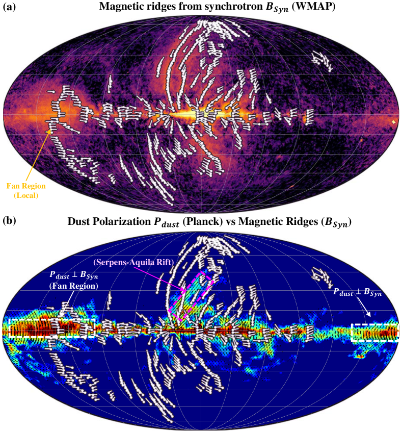
Figure 1: Extended Data Figure 1 $\mid$ Comparison between dust and synchrotron polarization. (a) Magnetic field ridges detected by synchrotron polarization ($B_{syn}$, WMAP at 22.8 GHz). The coherent ridges are enhanced in their polarized synchrotron intensity and connected by the magnetic field lines. (b) Comparison between thermal dust polarization ($P_{Dust}$,background black bars for direction and filled color for polarized intensity by Planck at 353 GHz[32]) and the magnetic ridges deduced from synchrotron (white lines adapted from panel  a). The dust polarization shows a general perpendicular direction to the magnetic field from synchrotron in the Galactic plane ($\mid b\mid<5^{\circ}$), while some of the dust polarization is parallel to the magnetic field in the known local structure within the Serpens-Aquila Rift. However, most of the magnetic ridges presented in (a) have no dust counterparts, hence they are Galactic structures.

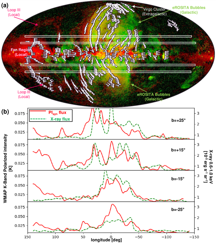
Figure 2: Extended Data Figure 2 $\mid$ Comparison between the X-ray surface brightness of the eROSITA Bubbles (0.6-1.0 keV) and the magnetic ridges. Panel  (a) presents the magnetic ridges from Figure 1(b), with four same-latitude cuts at the roots of the eROSITA Bubbles. The comparison between the polarized intensity WMAP-K Band[74] (PI_syn, red) and the 0.6-1.0 keV eROSITA[8] X-ray emission (green) for the four cuts are presented in panel  (b). The detected magnetic ridges are clear peaks of the red curves in (b). There is a good correlation between the edges of the eROSITA Bubbles in X-ray and the enhancements of the polarized synchrotron intensity (PI_syn,max). While the large-scale magnetic structures surrounding the northern cap of the eROSITA Bubble appear to largely enclose the Bubble, the same is not obviously true for the southern eROSITA Bubble; there, only the southeastern magnetic ridge approaches the cap of the southern eROSITA Bubble.

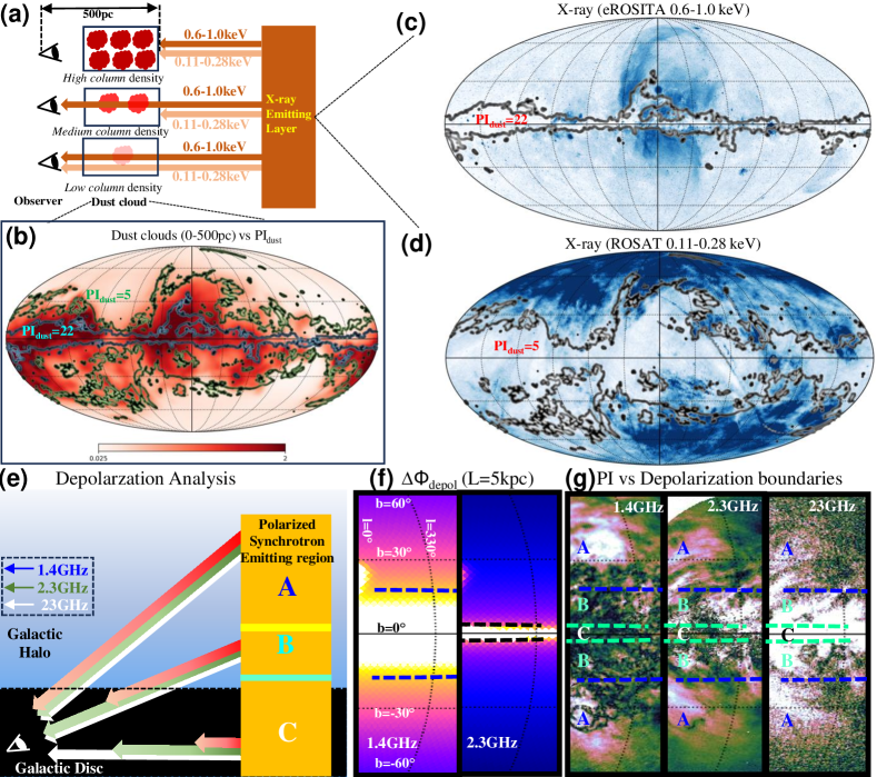
Figure 3: Extended Data Figure 3 $\mid$ the eROSITA Bubbles and the magnetised outflows are not local structures. The plots show how the distance of the X-ray (panels a-d) and polarized emission structures (panels e-g) are estimated. The X-ray absorption depends on the column density of the foreground medium (a). Panel b: The extinction map by the layer at 0-500 pc, as obtained from the 3D dust distribution by the Gaia-2MASS-Apogee dataset[19] (background image), matches the polarized dust intensity map at 353 GHz from Planck[32] (Contours are two levels of polarized intensity, $\mathrm{PI_{dust}}$). An anti-correlation is obvious between high dust column density (panel c, contours, $\mathrm{PI_{dust}}=22\mu$K) with high-energy X-ray emission (0.6-1.0 keV), and between low dust column density (panel d, contour, $\mathrm{PI_{dust}}=5\mu$K) with low energy X-ray (0.11-0.28 keV). Panel (e): For the polarized synchrotron emission, assuming the Galactic turbulent magnetic field out to 5-kpc, Faraday rotation depolarization is negligible at 22.8 GHz (WMAP map). The depolarization occurs up to a few degrees of Galactic latitude at 2.3 GHz (S-PASS), and further extends up to a Galactic latitude of $|b|\approx 20^{\circ}$ at 1.4 GHz (GMIMS) (see Extended Data Figure 4). The depolarization screen at 5 kpc is shown in (f) for the two lowest frequencies as the latitude at which the depolarization is 0.5 and $\Delta\Phi\simeq 40^{\circ}$. The observed polarized intensity maps are compared in (g). The observations are consistent with an origin of the polarized synchrotron emission at mid/high Galactic latitudes from beyond 5 kpc.

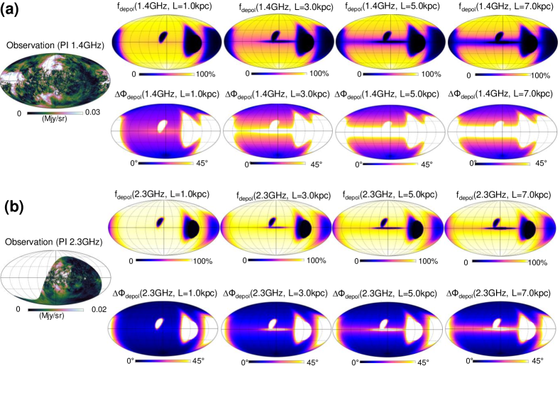
Figure 4: Extended Data Figure 4 $\mid$ Faraday depolarization by the turbulent Galactic magnetic field out to different distances from the Sun. $\mid$ The first column is the observed polarized emission at 1.4 GHz (a) and 2.3 GHz (b). Columns 2–5 are the Faraday depolarization $f_{depol}$ and angle dispersion $\Delta\Phi$ estimated as described in Methods and generated by the turbulent component of the Galactic magnetic field out to 1–7 kpc from us, respectively, at 1.4 GHz (top) and 2.3 GHz (bottom). The white color in $\Delta\Phi$ maps indicates the dispersion angles are expected to be more than $45^{\circ}$. At 1.4 GHz frequency, the depolarization screen shows significant growth in latitude between $L=1$–5 kpc. The $L=5$-kpc case can give the observed depolarization and the emission at mid and high Galactic latitudes, and hence the radiations of the magnetic ridges have to come from a distance beyond 5 kpc.

Supplementary

Radio data in SED analysis

We calculate the noise through the accuracy by (taking patch R1 subtracted by patch R2 as an example):

$$\begin{array}[]{ll}Signal:&I_{signal}=I_{R1}-I_{R2}\\ Noise:&s_{noise,accu}=R_{accuracy}\cdot\sqrt{(I_{R1})^{2}+(I_{R2})^{2}}\\ \end{array}$$ (16)

If the accuracy is high, we get the error from the beam sensitivity ($S_{beam}$) by:

$$\begin{array}[]{ll}s_{noise,sens}&=\frac{S_{beam}}{\sqrt{N_{beam}}}\\ &=\frac{S_{beam}}{\sqrt{A_{all}/A_{beam}}}\\ &=\frac{S_{beam}}{\sqrt{(N_{pix,all}*A_{pix})/(1.13*FWHM^{2})}}\\ \end{array}$$ (17)

We list the data and two types of errors in the Supplementary Table 1 from all 5 patches, and R1-R2, R3-R4, R5-R3 subtractions.

We convert the radio data from temperature T[K] to the spectral flux density $\mathcal{F}(\nu)$[MJy/sr] by

$$\mathcal{F}(\nu)[{\rm MJy/sr}]=\frac{T[{\rm K}]\cdot r_{fac}[{\rm Jy/K}]}{10^{6}{\rm Jy/MJy}}\frac{3283{\rm deg^{2}/sr}}{1.13\cdot(FWHM)^{2}{\rm deg^{2}}},$$ (18)

where $r_{fac}$ is the convert factor.

For radio data, we summarize the conversion methodologies below:

For 0.408 GHz, we use the 2014-Reprocessed Haslam 408 MHz[28] from [Ref.[48, 49]], $r_{fac}=5114$ Jy/sr K^-1, accuracy $10\%$.

For 1.4 GHz, we use the Stockert/DRAO survey[98, 99], $r_{fac}=11.25Jy/K$, accuracy $5\%$.

For 11 GHz, we use the Quijote survey[30], $r_{fac}=\frac{1}{961.9\mu K/Jy}$, accuracy $5\%$.

For 13 GHz, we use the Quijote survey[30], $r_{fac}=\frac{1}{703.8\mu K/Jy}$, accuracy $5\%$.

For 23 GHz, we use the synchrotron separation from WMAP[52] for data and error, $r_{fac}=\frac{1}{250.6\mu{K}/Jy}$.

For 30 GHz, we use the synchrotron separation from Planck survey[32]. $r_{fac}=24.33$ MJy/sr$\cdot$K^-1.

Note that for 23 GHz and 30 GHz, we use the synchrotron component from WMAP[74] and Planck[32] surveys, respectively.

X-ray-emitting halo re-analysis

As a pure geometric check, we try to test the expected X-ray emission maps from the “Bouquet Model”. We take the surface brightness measured from the paper of Predehl+2020[8] (here after P20) by taking the all-sky map in 0.6-1.0 keV energy band. The observed X-ray flux is assumed to be produced by the emission of thermal collision of hot plasma with the temperature of $T$ (with the emissivity of $\epsilon(T)$), and the observed surface brightness along the direction (l,b) can be expressed by (from [Ref.[100]]):

$$I_{X}(l,b)\propto\int dl_{depth}n_{H}^{2}\epsilon(T).$$ (19)

And the averaged surface brightness of the Bubbles is:

$$B_{X}\propto\frac{\int\int dl_{depth}d\theta\cdot n_{H}^{2}\epsilon(T)}{\Omega_{Bubble}},\\$$ (20)

where $l_{depth}$ is the emitting depth, $d\theta$ is the solid angle for the size of a pixel, $k_{B}$ is Boltzman’s constant, and $\Omega_{Bubble}$ is the solid angle of the emitting region observed in the sky. In our work, the outer outflows is modelled by the “Bouquet Model”, which we simplify into the following geometry (Supplemenatary Figure 4a) as an example: we assume the outer outflow in each side of the Galactic disc has the shape of an up-side-down truncated cone with a vacant cylindrical center. The radius at the bottom is 5 kpc and at the top is 8 kpc. The vacant cylinder has a radius of 3 kpc. The geometry in the disc is an annulus as extended as the star-forming ring of the Milky Way extending approximately at 3-5 kpc Galactic Centric. The contribution of the Fermi Bubbles are not considered in the modelling.

As a comparison, we also rebuild the P20 model, where the outer eROSITA Bubbles are modelled two spherical bubble shells with the outer radius of 7 kpc and different inner radius were tested (see Extended Data Figure). Here we reproduce the P20 modelling by two cases: 1) inner radius at 3 kpc (denoted as P20 model); 2) inner radius at 5 kpc (denoted as P20 thin model). In Supplementary Figure 4, we show the geometry of the modellings and their projected surface brightness in the all-sky map. In comparison, we compare the modelling the X-ray observation from 0.6-1.0 keV in the longitude cut at $l=10^{\circ}$ (In Supplementary Figure 4g) and $l=340^{\circ}$ (In Supplementary Figure 4h).

We consider the averaged surface brightness resulted from the “ Bouquet Model” is the same as what measured for the eROSITA Bubbles but the emitting geometry is defined by the new modelling ($B_{X,new}=B_{X,P20}$). We assume that in the “Bouquet Model”, the density is uniform, the temperature and the metallicity in the outer outflow are the same as P20 (T=0.3 keV, metallicity is 0.2 solar). The total energy in the emitting plasma can be estimated by $E_{tot}=n_{H}k_{B}TV$, where $V$ is the volume of the emitting plasma. Hence, we obtain the total energy in the outer outflow ($E_{tot,new}$) based on the total energy calculation based on the P20 modelling:

$$\begin{array}[]{ll}\frac{\int\int dl_{depth}d\theta_{new}}{\int d\theta}\cdot&\frac{E_{tot,new}^{2}}{V_{new}^{2}}=\frac{\int\int dl_{depth}d\theta_{old}}{\int d\theta}\cdot\frac{E_{tot,P20}^{2}}{V_{old}^{2}}\\ &\frac{E_{tot,new}}{E_{tot,P20}}=\frac{V_{new}/\sqrt{\int\int dl_{depth}d\theta_{new}/\Omega_{new}}}{V_{old}/\sqrt{\int\int dl_{depth}d\theta_{old}/\Omega_{old}}}\\ \end{array}$$ (21)

Here, $\int dl_{depth}$ is the length depth along different lines-of-sight, and $\int d\theta$ is the sky area that the projected model occupies. The footnote “new” is for the “Bouquet Model” and “P20” is for the P20 model. The energy for different Bouquet heights are summarized in Extended Data Table 2.

We make comparison for the observed surface brightness in Supplementary Figure 4(d-h), with the three modellings: 1) the “Bouquet Model” (height at 4 kpc); 2) P20 model (inner radius 3 kpc); 3) P20 thin model (inner radius 5 kpc). It is not surprising that the inner part ($l\lesssim 15^{\circ}$) shows lower surface brightness in our model when compared with the data. Indeed, we attribute such mismatch to the contribution from the Fermi Bubbles which have been observed to have enhanced X-ray emission at the roots[101, 35, 102]. For the cut of the outer outflow ($l=-30^{\circ}$), the lower-/mid-latitudes ($\mid b\mid<45^{\circ}$) are better reproduced by the “Bouquet Model”. Also, the southern sky is better reproduced by the “Bouquet Model” comparing to the previous models. On the other hand, the enhancement in the northern sky at high latitude (in NPS) is better reproduced by P20 thin model and is not present in the “Bouquet Model”. This indicates that either part of X-ray emission from the NPS is not associated with the Galactic outflows or that the NPS requires additional explanation in the “Bouquet Model”.

Remarks on the electron density model selections

We note that the electron distribution from “ymw16”[78] uses the dispersion measure of pulsars and fast radio bursts and includes the components such as the spiral arms, thin and thick disc. Hence, the “ymw16” model is advantageous to represent the electron distribution within the Galactic disc. This is suitable for the calculations in this section of the Faraday rotation depolarization analysis due to the Galactic disc as foreground. However, the “ymw16” model does not contain the component of X-ray-emitting warm-hot plasma in the circumgalactic medium beyond the Galactic disc. In our plasma-beta calculations for the halo presented in the main text, we employed the latest electron distribution data [Ref.[34]], derived from an analysis of X-ray observations conducted with eROSITA. [Ref.[34]] model the warm-hot plasma density at moderate-high Galactic latitudes and towards the anti-center direction. We extrapolate their analytic model towards the central regions of the Galaxy. We note that the Galactic outflows possibly introduce a deviation in the central regions of the Milky Way. We calculate the plasma-beta by $\beta\equiv p_{th}/p_{B}$, where the magnetic pressure is $p_{B}=\frac{B^{2}}{8\pi}$ and the thermal pressure is $p_{th}=n_{e}k_{B}T$. If we adopt a smaller electron density in the eROSITA Bubbles following [Ref.[8]] ($2\times 10^{-3}$ cm^-3), the plasma betas are $\beta_{r1}\simeq 6$ and $\beta_{r3}\simeq 12$, respectively. Patches R1 and R3 in the outer outflows are still in high plasma beta regime.

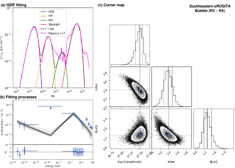
Figure 2: Supplementary Figure 2 $\mid$ The fitting details for southeastern outer outflows. Same as Supplementary Figure 1 but for the SED fitting in Figure 2d for the patch R3 - patch R4. The data dispersion is within 1-$\sigma$ to the best fit. The Gaussian distribution for all the three parameters have been reached.

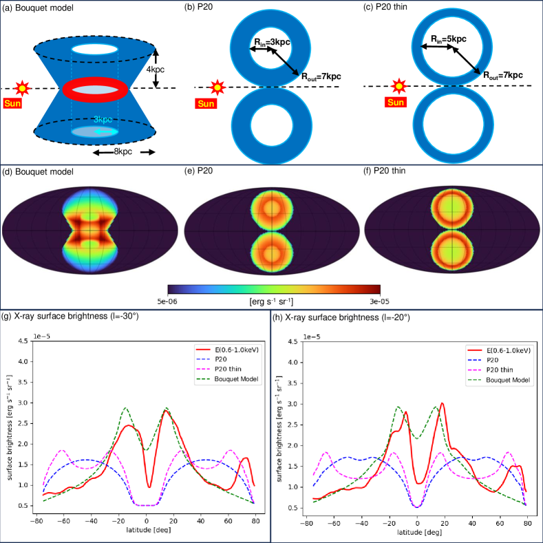
Figure 4: Supplementary Figure 4 $\mid$ The comparison between the “Bouquet Model” and the “P20” Model. The geometries are described in (a) the simplified “Bouquet Model” with upper radius $8$ kpc, the root with 5 kpc Galactic Centric, and the height of 4 kpc. (b) “P20” Model with the inner radius of 3 kpc and the outer radius of 7 kpc; (c) “P20 thin” Model with the inner radius of 5 kpc and the outer radius of 7 kpc. The expected X-ray emitting maps for 0.6-1.0 keV are presented in (d-f). Positive longitude is influenced by the dust absorption (see Extended Data Figure 3d) so it is not included. Eastern cuts are presented at (g) $l=30^{\circ}$ and (h) $l=20^{\circ}$ for the X-ray fluxes at 0.6-1.0 keV for eROSITA measurement (red), the “Bouquet Model” (green), “P20” Model (blue), and “P20 thin” Model (magenta). (h) western cuts at $l=340^{\circ}$. The “Bouquet Model” predicts a decreasing gradient for the X-ray flux from the disc upwards, which provides a clear better fit at low-/mid-latitudes ($\mid b\mid<45^{\circ}$) and the whole southern sky. In the north side of the North Polar Spur (NPS), the P20 thin model is better. In fact, the P20 thin model always predicts a large enhancement at high Galactic latitudes, which is only observed in the NPS.

$0.408$ GHz	patch R1	patch R2	patch R3	patch R4	patch R5	R1-R2	R3-R4	R5-R3
Signal	0.20494	0.10305	0.13333	0.08102	0.14737	0.10189	0.05231	0.01404
Erraccuracy	0.01025	0.00515	0.00667	0.00405	0.00737	0.01147	0.00780	0.00994
Errsensitivity	0.00038	0.00044	0.00033	0.00037	0.00037	0.00058	0.00050	0.00050
$1.4$ GHz	patch R1	patch R2	patch R3	patch R4	patch R5	R1-R2	R3-R4	R5-R3
Signal	0.09191	0.05230	0.07704	0.06887	0.08884	0.03961	0.00817	0.01180
Erraccuracy	0.00460	0.00261	0.00385	0.00344	0.00444	0.00529	0.00517	0.00588
Errsensitivity	0.00022	0.00025	0.00019	0.00022	0.00022	0.00034	0.00029	0.00029
$11$ GHz	patch R1	patch R2	patch R3	patch R4	patch R5	R1-R2	R3-R4	R5-R3
Signal	0.04198	0.04094	null	null	null	0.00103	null	null
Erraccuracy	0.00210	0.00205	null	null	null	0.00293	null	null
Errsensitivity	0.00002	0.00002	null	null	null	0.00003	null	null
$13$ GHz	patch R1	patch R2	patch R3	patch R4	patch R5	R1-R2	R3-R4	R5-R3
Signal	0.03908	0.03851	null	null	null	0.00057	null	null
Erraccuracy	0.00195	0.00193	null	null	null	0.00274	null	null
Errsensitivity	0.00002	0.00002	null	null	null	0.00003	null	null
$23$ GHz syn	patch R1	patch R2	patch R3	patch R4	patch R5	R1-R2	R3-R4	R5-R3
Signal	0.00172	0.00041	0.00103	0.00045	0.00137	0.00131	0.00058	0.00034
Errtot	0.00044	0.00020	0.00039	0.00025	0.00054	0.00049	0.00046	0.00067
$30$ GHz syn	patch R1	patch R2	patch R3	patch R4	patch R5	R1-R2	R3-R4	R5-R3
Signal	0.00173	0.00061	0.00084	0.00051	0.00099	0.00112	0.00033	0.00015
Erraccuracy	0.00009	0.00003	0.00004	0.00003	0.00005	0.00009	0.00005	0.00007
Errsensitivity	0.00009	0.00011	0.00008	0.00009	0.00009	0.00014	0.00012	0.00012

Table 3: Supplementary Table 1 $\mid$ Radio data for SED analysis. References for the data survey are listed in the Methods. Errors from accuracy and errors from sensitivity are listed with units  MJy/sr. The patches are listed in Figure 2.

Affiliations

1. INAF - Osservatorio Astronomico di Brera, via E. Bianchi 46, 23807 Merate (LC), Italy; e-mail: heshou.zhang@inaf.it; gabriele.ponti@inaf.it; carretti@ira.inaf.it; ryliu@nju.edu.cn; morris@astro.ucla.edu

2. Max-Planck-Institut für Extraterrestrische Physik (MPE), Giessenbachstrasse 1, 85748 Garching bei München, Germany;

3. INAF Istituto di Radioastronomia, Via Gobetti 101, I-40129 Bologna, Italy;

4. School of Astronomy and Space Science, Xianlin Road 163, Nanjing University, Nanjing 210023, People’s Republic of China;

5. Key Laboratory of Modern Astronomy and Astrophysics (Nanjing University), Ministry of Education, Nanjing 210023, People’s Republic of China;

6. University of California Los Angeles, Los Angeles, CA, USA;

7. Department of Astrophysics/IMAPP, Radboud University Nijmegen, P.O. Box 9010, 6500 GL Nijmegen, The Netherlands;

8. Dublin Institute for Advanced Studies, 31 Fitzwilliam Place, Dublin 2, Ireland;

9. Max-Planck-Institut für Kernphysik, P.O. Box 103980, D-69029 Heidelberg, Germany;

10. Yerevan State University, 1 Alek Manukyan St, Yerevan 0025, Armenia;

11. DiSAT, Università degli Studi dell’Insubria, via Valleggio 11, 22100 Como, Italy;

Acknowledgements

HZ acknowledges support by the X-riStMAs project (Seal of Excellence n. [0000153]) under the National Recovery and Resilience Plan (PNRR), Mission 4, Component 2, Investment 1.2 - Italian Ministry of University and Research, funded by the European Union – NextGenerationEU. HZ also acknowledges the computing support from PLEIADI supercomputer from INAF. HZ, GP, NL, XZ, YZ, GS acknowl- edge financial support from the European Research Council (ERC) un- der the European Union’s Horizon 2020 research and innovation pro- gram HotMilk (grant agreement No. [865637]). GP also aknowledges support from Bando per il Finanziamento della Ricerca Fondamentale 2022 dell’Istituto Nazionale di Astrofisica (INAF): GO Large program and from the Framework per l’Attrazione e il Rafforzamento delle Ec- cellenze (FARE) per la ricerca in Italia (R20L5S39T9).

References

- [1] Krause, M. Magnetic Fields and Halos in Spiral Galaxies. Galaxies 7, 54 (2019).
- [2] Krause, M. et al. CHANG-ES. XXII. Coherent magnetic fields in the halos of spiral galaxies. Astron. Astrophys. 639, A112 (2020).
- [3] Heesen, V., Krause, M., Beck, R. & Dettmar, R. J. Cosmic rays and the magnetic field in the nearby starburst galaxy NGC 253. II. The magnetic field structure. Astron. Astrophys. 506, 1123–1135 (2009).
- [4] Moss, D., Sokoloff, D., Beck, R. & Krause, M. Galactic winds and the symmetry properties of galactic magnetic fields. Astron. Astrophys. 512, A61 (2010).
- [5] Manna, S. & Roy, S. Magnetic Fields, Star Formation Rates, and Gas Densities at Sub-kiloparsec Scales in a Pilot Sample of Nearby Galaxies. Astrophys. J. 944, 86 (2023).
- [6] Carretti, E. et al. Giant magnetized outflows from the centre of the Milky Way. Nature 493, 66–69 (2013).
- [7] Wolleben, M. et al. The Global Magneto-ionic Medium Survey: A Faraday Depth Survey of the Northern Sky Covering 1280-1750 MHz. Astron. J. 162, 35 (2021).
- [8] Predehl, P. et al. Detection of large-scale X-ray bubbles in the Milky Way halo. Nature 588, 227–231 (2020).
- [9] Yang, H. Y. K., Ruszkowski, M. & Zweibel, E. G. Fermi and eROSITA bubbles as relics of the past activity of the Galaxy’s central black hole. Nature Astronomy 6, 584–591 (2022).
- [10] Sarkar, K. C., Mondal, S., Sharma, P. & Piran, T. Misaligned Jets from Sgr A* and the Origin of Fermi/eROSITA Bubbles. Astrophys. J. 951, 36 (2023).
- [11] Nguyen, D. D. & Thompson, T. A. Galactic Winds and Bubbles from Nuclear Starburst Rings. Astrophys. J. Lett. 935, L24 (2022).
- [12] Strickland, D. K., Heckman, T. M., Colbert, E. J. M., Hoopes, C. G. & Weaver, K. A. A High Spatial Resolution X-Ray and H Study of Hot Gas in the Halos of Star-forming Disk Galaxies. I. Spatial and Spectral Properties of the Diffuse X-Ray Emission. Astrophys. J. S. 151, 193–236 (2004).
- [13] Strickland, D. K. & Heckman, T. M. Iron Line and Diffuse Hard X-Ray Emission from the Starburst Galaxy M82. Astrophys. J. 658, 258–281 (2007).
- [14] Krause, M. Magnetic Fields and Halos in Spiral Galaxies. Galaxies 7, 54 (2019).
- [15] Hinshaw, G. et al. Nine-year Wilkinson Microwave Anisotropy Probe (WMAP) Observations: Cosmological Parameter Results. Astrophys. J., Suppl. Ser. 208, 19 (2013).
- [16] Vidal, M., Dickinson, C., Davies, R. D. & Leahy, J. P. Polarized radio filaments outside the Galactic plane. Mon. Not. R. Astron. Soc. 452, 656–675 (2015).
- [17] Liu, W. et al. The Structure of the Local Hot Bubble. Astrophys. J. 834, 33 (2017).
- [18] Berkhuijsen, E. M., Haslam, C. G. T. & Salter, C. J. Are the galactic loops supernova remnants? Astron. Astrophys. 14, 252 (1971).
- [19] Lallement, R. et al. Three-dimensional maps of interstellar dust in the Local Arm: using Gaia, 2MASS, and APOGEE-DR14. Astron. Astrophys. 616, A132 (2018).
- [20] Burn, B. J. On the depolarization of discrete radio sources by Faraday dispersion. Mon. Not. R. Astron. Soc. 133, 67 (1966).
- [21] Tribble, P. C. Depolarization of extended radio sources by a foreground Faraday screen. Mon. Not. R. Astron. Soc. 250, 726 (1991).
- [22] Sokoloff, D. D. et al. Depolarization and Faraday effects in galaxies. Mon. Not. R. Astron. Soc. 299, 189–206 (1998).
- [23] Platz, L. I. et al. Multi-Component Imaging of the Fermi Gamma-ray Sky in the Spatio-spectral Domain. arXiv e-prints arXiv:2204.09360 (2022).
- [24] Dobler, G., Finkbeiner, D. P., Cholis, I., Slatyer, T. & Weiner, N. The Fermi Haze: A Gamma-ray Counterpart to the Microwave Haze. Astrophys. J. 717, 825–842 (2010).
- [25] Planck Collaboration et al. Planck intermediate results. IX. Detection of the Galactic haze with Planck. Astron. Astrophys. 554, A139 (2013).
- [26] Lacki, B. C. The Fermi bubbles as starburst wind termination shocks. Mon. Not. R. Astron. Soc. 444, L39–L43 (2014).
- [27] Crocker, R. M., Bicknell, G. V., Taylor, A. M. & Carretti, E. A Unified Model of the Fermi Bubbles, Microwave Haze, and Polarized Radio Lobes: Reverse Shocks in the Galactic Center’s Giant Outflows. Astrophys. J. 808, 107 (2015).
- [28] Remazeilles, M., Dickinson, C., Banday, A. J., Bigot-Sazy, M. A. & Ghosh, T. An improved source-subtracted and destriped 408-MHz all-sky map. Mon. Not. R. Astron. Soc. 451, 4311–4327 (2015).
- [29] Wolleben, M., Landecker, T. L., Reich, W. & Wielebinski, R. An absolutely calibrated survey of polarized emission from the northern sky at 1.4 GHz. Observations and data reduction. Astron. Astrophys. 448, 411–424 (2006).
- [30] Rubiño-Martín, J. A. et al. QUIJOTE scientific results - IV. A northern sky survey in intensity and polarization at 10-20 GHz with the multifrequency instrument. Mon. Not. R. Astron. Soc. 519, 3383–3431 (2023).
- [31] Fuskeland, U., Wehus, I. K., Eriksen, H. K. & Næss, S. K. Spatial Variations in the Spectral Index of Polarized Synchrotron Emission in the 9 yr WMAP Sky Maps. Astrophys. J. 790, 104 (2014).
- [32] Planck Collaboration et al. Planck 2018 results. IV. Diffuse component separation. Astron. Astrophys. 641, A4 (2020).
- [33] Ajello, M. et al. Fermi Large Area Telescope Performance after 10 Years of Operation. Astrophys. J. S. 256, 12 (2021).
- [34] Locatelli, N. et al. The warm-hot circumgalactic medium of the Milky Way as seen by eROSITA. Astron. Astrophys. 681, A78 (2024).
- [35] Su, M., Slatyer, T. R. & Finkbeiner, D. P. Giant Gamma-ray Bubbles from Fermi-LAT: Active Galactic Nucleus Activity or Bipolar Galactic Wind? Astrophys. J. 724, 1044–1082 (2010).
- [36] Elia, D. et al. The Star Formation Rate of the Milky Way as Seen by Herschel. Astrophys. J. 941, 162 (2022).
- [37] Chevalier, R. A. & Clegg, A. W. Wind from a starburst galaxy nucleus. Nature 317, 44–45 (1985).
- [38] Heckman, T. M., Lehnert, M. D., Strickland, D. K. & Armus, L. Absorption-Line Probes of Gas and Dust in Galactic Superwinds. Astrophys. J., Suppl. Ser. 129, 493–516 (2000).
- [39] Veilleux, S., Cecil, G. & Bland-Hawthorn, J. Galactic Winds. Annu. Rev. Astron. Astrophys. 43, 769–826 (2005).
- [40] Strickland, D. K. & Heckman, T. M. Supernova Feedback Efficiency and Mass Loading in the Starburst and Galactic Superwind Exemplar M82. Astrophys. J. 697, 2030–2056 (2009).
- [41] Vink, J. & Yamazaki, R. A Critical Shock Mach Number for Particle Acceleration in the Absence of Pre-existing Cosmic Rays: . Astrophys. J. 780, 125 (2014).
- [42] Guo, X., Sironi, L. & Narayan, R. Electron Heating in Low Mach Number Perpendicular Shocks. II. Dependence on the Pre-shock Conditions. Astrophys. J. 858, 95 (2018).
- [43] Marasco, A. & Fraternali, F. Modelling the H I halo of the Milky Way. Astron. Astrophys. 525, A134 (2011).
- [44] Faerman, Y., Sternberg, A. & McKee, C. F. Massive Warm/Hot Galaxy Coronae as Probed by UV/X-Ray Oxygen Absorption and Emission. I. Basic Model. Astrophys. J. 835, 52 (2017).
- [45] Sancisi, R., Fraternali, F., Oosterloo, T. & van Moorsel, G. The Vertical Structure and Kinematics of HI in Spiral Galaxies. In Funes, J. G. & Corsini, E. M. (eds.) Galaxy Disks and Disk Galaxies, vol. 230 of Astronomical Society of the Pacific Conference Series, 111–118 (2001).
- [46] Marasco, A., Marinacci, F. & Fraternali, F. On the origin of the warm-hot absorbers in the Milky Way’s halo. Mon. Not. R. Astron. Soc. 433, 1634–1647 (2013).
- [47] Meliani, Z. et al. The galactic bubbles of starburst galaxies The influence of galactic large-scale magnetic fields. arXiv e-prints arXiv:2402.01541 (2024).
- [48] Haslam, C. G. T. NOD2 A General System of Analysis for Radioastronomy. Astron. Astrophys. Suppl. 15, 333 (1974).
- [49] Haslam, C. G. T., Salter, C. J., Stoffel, H. & Wilson, W. E. A 408 MHz all-sky continuum survey. II. The atlas of contour maps. Astronomy and Astrophysics, Suppl. Ser. 47, 1–143 (1982).
- [50] Testori, J. C., Reich, P. & Reich, W. A fully sampled 21 cm linear polarization survey of the southern sky. Astron. Astrophys. 484, 733–742 (2008).
- [51] Carretti, E. et al. S-band Polarization All-Sky Survey (S-PASS): survey description and maps. Mon. Not. R. Astron. Soc. 489, 2330–2354 (2019).
- [52] Bennett, C. L. et al. Nine-year Wilkinson Microwave Anisotropy Probe (WMAP) Observations: Final Maps and Results. Astrophys. J., Suppl. Ser. 208, 20 (2013).
- [53] Planck Collaboration et al. Planck 2018 results. IV. Diffuse component separation. Astron. Astrophys. 641, A4 (2020).
- [54] Planck Collaboration et al. Planck 2018 results. XI. Polarized dust foregrounds. Astron. Astrophys. 641, A11 (2020).
- [55] Abdollahi, S. et al. Incremental Fermi Large Area Telescope Fourth Source Catalog. Astrophys. J. S. 260, 53 (2022).
- [56] Hona, B., Robare, A., Fleischhack, H., Huentemeyer, P. & HAWC Collaboration. Correlated GeV-TeV Gamma-Ray Emission from Extended Sources in the Cygnus Region. In 35th International Cosmic Ray Conference (ICRC2017), vol. 301 of International Cosmic Ray Conference, 710 (2017).
- [57] Snowden, S. L. et al. ROSAT Survey Diffuse X-Ray Background Maps. II. Astrophys. J. 485, 125–135 (1997).
- [58] Van Rossum, G. & Drake, F. L. Python 3 Reference Manual (CreateSpace, Scotts Valley, CA, 2009).
- [59] van der Walt, S., Colbert, S. C. & Varoquaux, G. The NumPy Array: A Structure for Efficient Numerical Computation. Computing in Science and Engineering 13, 22–30 (2011).
- [60] Harris, C. R. et al. Array programming with NumPy. Nature 585, 357–362 (2020). URL https://doi.org/10.1038/s41586-020-2649-2.
- [61] Górski, K. M. et al. HEALPix: A Framework for High-Resolution Discretization and Fast Analysis of Data Distributed on the Sphere. Astrophys. J. 622, 759–771 (2005).
- [62] Zonca, A. et al. healpy: equal area pixelization and spherical harmonics transforms for data on the sphere in python. Journal of Open Source Software 4, 1298 (2019). URL https://doi.org/10.21105/joss.01298.
- [63] Astropy Collaboration et al. Astropy: A community Python package for astronomy. Astron. Astrophys. 558, A33 (2013).
- [64] Astropy Collaboration et al. The Astropy Project: Building an Open-science Project and Status of the v2.0 Core Package. Astron. J. 156, 123 (2018).
- [65] Astropy Collaboration et al. The Astropy Project: Sustaining and Growing a Community-oriented Open-source Project and the Latest Major Release (v5.0) of the Core Package. Astrophys. J. 935, 167 (2022).
- [66] Wood, M. et al. Fermipy: An open-source Python package for analysis of Fermi-LAT Data. In 35th International Cosmic Ray Conference (ICRC2017), vol. 301 of International Cosmic Ray Conference, 824 (2017).
- [67] Kluyver, T. et al. Jupyter notebooks ? a publishing format for reproducible computational workflows. In Loizides, F. & Scmidt, B. (eds.) Positioning and Power in Academic Publishing: Players, Agents and Agendas, 87–90 (IOS Press, 2016). URL https://eprints.soton.ac.uk/403913/.
- [68] Hunter, J. D. Matplotlib: A 2D Graphics Environment. Computing in Science and Engineering 9, 90–95 (2007).
- [69] Joye, W. A. & Mandel, E. New Features of SAOImage DS9. In Payne, H. E., Jedrzejewski, R. I. & Hook, R. N. (eds.) Astronomical Data Analysis Software and Systems XII, vol. 295 of Astronomical Society of the Pacific Conference Series, 489 (2003).
- [70] Maconi, E. et al. Modelling Local Bubble analogs: synthetic dust polarization maps. Mon. Not. R. Astron. Soc. 523, 5995–6010 (2023).
- [71] Frisch, P. C., Redfield, S. & Slavin, J. D. The Interstellar Medium Surrounding the Sun. Annu. Rev. Astron. Astrophys. 49, 237–279 (2011).
- [72] Yeung, M. C. H. et al. SRG/eROSITA X-ray shadowing study of giant molecular clouds. Astron. Astrophys. 676, A3 (2023).
- [73] Beck, R. Magnetic fields in spiral galaxies. Astron. Astrophys. Rev. 24, 4 (2015).
- [74] Bennett, C. L. et al. Nine-year Wilkinson Microwave Anisotropy Probe (WMAP) Observations: Final Maps and Results. Astrophys. J., Suppl. Ser. 208, 20 (2013).
- [75] Ehle, M. & Beck, R. Ionized gas and intrinsic magnetic fields in the spiral galaxy NGC 6946. Astron. Astrophys. 273, 45–64 (1993).
- [76] Armstrong, J. W., Rickett, B. J. & Spangler, S. R. Electron Density Power Spectrum in the Local Interstellar Medium. Astrophys. J. 443, 209 (1995).
- [77] Chepurnov, A. & Lazarian, A. Extending the Big Power Law in the Sky with Turbulence Spectra from Wisconsin H Mapper Data. Astrophys. J. 710, 853–858 (2010).
- [78] Yao, J. M., Manchester, R. N. & Wang, N. A New Electron-density Model for Estimation of Pulsar and FRB Distances. Astrophys. J. 835, 29 (2017).
- [79] Jansson, R. & Farrar, G. R. The Galactic Magnetic Field. Astrophys. J. Lett. 761, L11 (2012).
- [80] Planck Collaboration et al. Planck intermediate results. XLII. Large-scale Galactic magnetic fields. Astron. Astrophys. 596, A103 (2016).
- [81] Carretti, E. et al. S-band Polarization All-Sky Survey (S-PASS): survey description and maps. Mon. Not. R. Astron. Soc. 489, 2330–2354 (2019).
- [82] Iacobelli, M. et al. Studying Galactic interstellar turbulence through fluctuations in synchrotron emission. First LOFAR Galactic foreground detection. Astron. Astrophys. 558, A72 (2013).
- [83] Popescu, C. C. et al. A radiation transfer model for the Milky Way: I. Radiation fields and application to high-energy astrophysics. Mon. Not. R. Astron. Soc. 470, 2539–2558 (2017).
- [84] Zabalza, V. naima: a python package for inference of relativistic particle energy distributions from observed nonthermal spectra. Proc. of International Cosmic Ray Conference 2015 922 (2015).
- [85] Aharonian, F. A., Kelner, S. R. & Prosekin, A. Y. Angular, spectral, and time distributions of highest energy protons and associated secondary gamma rays and neutrinos propagating through extragalactic magnetic and radiation fields. Phys. Rev. D 82, 043002 (2010).
- [86] Khangulyan, D., Aharonian, F. A. & Kelner, S. R. Simple Analytical Approximations for Treatment of Inverse Compton Scattering of Relativistic Electrons in the Blackbody Radiation Field. Astrophys. J. 783, 100 (2014).
- [87] Zirakashvili, V. N. & Aharonian, F. Analytical solutions for energy spectra of electrons accelerated by nonrelativistic shock-waves in shell type supernova remnants. Astron. Astrophys. 465, 695–702 (2007).
- [88] Ackermann, M. et al. A Cocoon of Freshly Accelerated Cosmic Rays Detected by Fermi in the Cygnus Superbubble. Science 334, 1103 (2011).
- [89] Heesen, V., Dettmar, R.-J., Krause, M., Beck, R. & Stein, Y. Advective and diffusive cosmic ray transport in galactic haloes. Mon. Not. R. Astron. Soc. 458, 332–353 (2016).
- [90] Heesen, V. The radio continuum perspective on cosmic-ray transport in external galaxies. Astrophy. S. S. 366, 117 (2021).
- [91] Reed, B. C. New Estimates of the Solar-Neighborhood Massive Star Birthrate and the Galactic Supernova Rate. Astron. J. 130, 1652–1657 (2005).
- [92] Diehl, R. et al. Radioactive 26Al from massive stars in the Galaxy. Nature 439, 45–47 (2006).
- [93] Li, W. et al. Nearby supernova rates from the Lick Observatory Supernova Search - III. The rate-size relation, and the rates as a function of galaxy Hubble type and colour. Mon. Not. R. Astron. Soc. 412, 1473–1507 (2011).
- [94] Rozwadowska, K., Vissani, F. & Cappellaro, E. On the rate of core collapse supernovae in the milky way. New Astro. 83, 101498 (2021).
- [95] Adams, S. M., Kochanek, C. S., Beacom, J. F., Vagins, M. R. & Stanek, K. Z. Observing the Next Galactic Supernova. Astrophys. J. 778, 164 (2013).
- [96] Poznanski, D. An emerging coherent picture of red supergiant supernova explosions. Mon. Not. R. Astron. Soc. 436, 3224–3230 (2013).
- [97] Fox, A. J. et al. The Mass Inflow and Outflow Rates of the Milky Way. Astrophys. J. 884, 53 (2019).
- [98] Reich, P. & Reich, W. A radio continuum survey of the northern sky at 1420 MHz. II. Astron. Astrophys. Suppl. 63, 205 (1986).
- [99] Reich, P., Testori, J. C. & Reich, W. A radio continuum survey of the southern sky at 1420 MHz. The atlas of contour maps. Astron. Astrophys. Suppl. 376, 861–877 (2001).
- [100] Miller, M. J. & Bregman, J. N. Constraining the Milky Way’s Hot Gas Halo with O VII and O VIII Emission Lines. Astrophys. J. 800, 14 (2015).
- [101] Bland-Hawthorn, J. & Cohen, M. The Large-Scale Bipolar Wind in the Galactic Center. Astrophys. J. 582, 246–256 (2003).
- [102] Ponti, G. et al. An X-ray chimney extending hundreds of parsecs above and below the Galactic Centre. Nature 567, 347–350 (2019).