LEARN: An Invex Loss for Outlier Oblivious Robust Online Optimization

Adarsh Barik
Institute of Data Science
National University of Singapore
Singapore, 117602
abarik@nus.edu.sg
&Anand Krishna
Department of Electrical and Computer Engineering
National University of Singapore
Singapore, 117583
akr@nus.edu.sg
&Vincent Y. F. Tan
Department of Mathematics
Department of Electrical and Computer Engineering
National University of Singapore
Singapore, 119077
vtan@nus.edu.sg
Abstract

We study a robust online convex optimization framework, where an adversary can introduce outliers by corrupting loss functions in an arbitrary number of rounds $k$, unknown to the learner. Our focus is on a novel setting allowing unbounded domains and large gradients for the losses without relying on a Lipschitz assumption. We introduce the Log Exponential Adjusted Robust and iNvex (Learn) loss, a non-convex (invex) robust loss function to mitigate the effects of outliers and develop a robust variant of the online gradient descent algorithm by leveraging the Learn loss. We establish tight regret guarantees (up to constants), in a dynamic setting, with respect to the uncorrupted rounds and conduct experiments to validate our theory. Furthermore, we present a unified analysis framework for developing online optimization algorithms for non-convex (invex) losses, utilizing it to provide regret bounds with respect to the Learn loss, which may be of independent interest.

1 Introduction

In the mercurial era of digital information, the proliferation of online data streams has become ubiquitous, with applications spanning from financial markets and healthcare to e-commerce and social mediaย (D.ย Hendricks and Wilcox,, 2016; Zhang etย al.,, 2015; Fedoryszak etย al.,, 2019; Kejariwal etย al.,, 2015). The surge in real-time data generation across these diverse fields has underscored the pressing need for adaptive optimization strategies. These strategies need to navigate dynamic and uncertain environments, especially as organizations rely more on online decision-making processes. In this context, the demand for efficient and robust optimization techniques in the presence of outliers has become more pronounced.

Outlier robustness

Pioneering works in robust statisticsย (Huber,, 1964; Beaton and Tukey,, 1974) emphasized mitigating outliersโ€™ impact on algorithm performance. In online optimization originally designed for uncorrupted streams, outliers pose challenges leading to suboptimal solutionsย (Feng etย al.,, 2017). This motivates developing outlier-robust online methodologies, an area of recent focusย (Diakonikolas etย al.,, 2022; van Erven etย al.,, 2021; Bhaskara and Ruwanpathirana,, 2020; Feng etย al.,, 2017).

Online convex optimization (OCO)

The OCO frameworkย (Hazan,, 2023; Orabona,, 2023) offers a useful mathematical framework for studying sequential predictions, especially in the presence of adversarial interventions. The adversary chooses a deterministic sequence of convex losses $f_{t}$ for each $t\in\{1,2,\ldots,T\}$, where $T$ denotes the time horizon. In every round, the learner picks an action $\theta_{t}$ in a convex set $\Theta$ for which she suffers the loss $f_{t}(\theta_{t})$ for the round $t$ and additionally gets to observe $f_{t}$. The learnerโ€™s goal is to minimize the cumulative loss, i.e., $\sum_{t=1}^{T}f_{t}(\theta_{t})$, and her performance is evaluated using the notion of regret.

OCO with robustness

The OCO framework serves as a valuable starting point for studying algorithms that dynamically adapt to incoming data points while considering potential outliersโ€™ influence. Drawing inspiration from the model proposed by van Erven etย al., (2021), this work considers the OCO framework where the adversary is allowed to choose any $\mathcal{S}\subseteq[T]$ of rounds to be โ€˜cleanโ€™ and inject outliers into the remaining rounds. This adversarial influence is exerted by tampering with the side information stsubscript๐‘ ๐‘กs_{t} integral to constructing the loss function $f_{t}$. Considering the example of the online ridge regression problem, where st=(xt,yt)subscript๐‘ ๐‘กsubscript๐‘ฅ๐‘กsubscript๐‘ฆ๐‘กs_{t}=(x_{t},y_{t}) represents the incoming data point for round $t$, and the loss is defined as ftโ€‹(st,ฮธt)=12โ€‹(โŸจฮธt,xtโŸฉโˆ’yt)2subscript๐‘“๐‘กsubscript๐‘ ๐‘กsubscript๐œƒ๐‘ก12superscriptsubscript๐œƒ๐‘กsubscript๐‘ฅ๐‘กsubscript๐‘ฆ๐‘ก2f_{t}(s_{t},\theta_{t})=\frac{1}{2}(\langle\theta_{t}\,,x_{t}\rangle-y_{t})^{2}, the adversary can corrupt either $x_{t}$, $y_{t}$ or both to corrupt the round $t$. The corrupted round is considered an outlier. We use $c_{t}$ to denote the uncorrupted side information and $o_{t}$ for the corrupted side information. The learnerโ€™s performance is measured using regret with respect to only the clean rounds, and we refer to this as clean regret. In this paper, we explore the notion of dynamic regret โ€“ a performance measure suitable for dynamic environments characterized by evolving data and shifting optimal decision parameters. Dynamic regret entails adapting strategies to compete effectively with evolving comparators, thereby mitigating the impact of changing environments on decision-making processes. Let $\bm{\theta}\coloneqq(\theta_{t})_{t\in[T]}$ be a sequence of learnerโ€™s actions and $(\omega^{*}_{t})_{t\in[T]}$ be a sequence of benchmark points such that ฯ‰tโˆ—=argโ€‹minฮธโˆˆฮ˜โกftโ€‹(st,ฮธ)superscriptsubscript๐œ”๐‘กsubscriptargmin๐œƒฮ˜subscript๐‘“๐‘กsubscript๐‘ ๐‘ก๐œƒ\omega_{t}^{*}=\operatorname*{arg\,min}_{\theta\in\Theta}f_{t}(s_{t},\theta). We also define $\theta_{t}^{*}=\operatorname*{arg\,min}_{\theta\in\Theta}f_{t}(c_{t},\theta)$. Clearly, $\theta_{t}^{*}=\omega_{t}^{*}$ for clean rounds. Then, the clean dynamic regret is defined to be

โ„œRDTโ€‹(๐œฝ,๐’ฎ)โ‰”โˆ‘tโˆˆ๐’ฎ(ftโ€‹(st,ฮธt)โˆ’ftโ€‹(st,ฮธtโˆ—)).โ‰”superscriptsubscriptโ„œRD๐‘‡๐œฝ๐’ฎsubscript๐‘ก๐’ฎsubscript๐‘“๐‘กsubscript๐‘ ๐‘กsubscript๐œƒ๐‘กsubscript๐‘“๐‘กsubscript๐‘ ๐‘กsubscriptsuperscript๐œƒ๐‘ก\displaystyle\mathfrak{R}_{\operatorname{RD}}^{T}(\bm{\theta},\mathcal{S})\coloneqq\sum_{t\in\mathcal{S}}\big{(}f_{t}(s_{t},\theta_{t})-f_{t}(s_{t},\theta^{*}_{t})\big{)}~{}. (1)

Our goal is to develop robust online algorithms to achieve sublinear regret with respect to $T$ and achieve optimal dependency on the number of outliers $k$, which is unknown.

Refer to caption
(a) $k=0$
Refer to caption
(b) $k=T^{\frac{2}{3}}$
Figure 1: We compared Learn (Algorithmย 1) and baselines (Sectionย 4) on binary classification with hinge loss and sequential data. Figureย 1(a) shows the true decision boundary with no outliers and all the methods recover it exactly. Figureย 1(b) shows how decision boundaries for baseline methods deviate from the ground truth in the presence of outliers while Learn remains robust to outliers.

This work focuses on $m$-strongly convex losses. Diverging from van Erven etย al., (2021)โ€™s static model, we introduce novel OCO techniques for outlier scenarios when the number of outliers $k$ is unknown. Unlike their work assuming known $k$, and in contrast to common bounded domain/Lipschitz loss assumptions (Hazan,, 2023; Orabona,, 2023), our approach allows unbounded domains and non-Lipschitz losses. Following Jacobsen and Cutkosky, (2023), we permit arbitrarily large gradients away from $f_{t}$โ€™s minimizer, extending applicability to outlier scenarios.

Table 1: Best known upper bounds on the dynamic regret of strongly convex loss functions $f_{t}$ in the presence of outliers (with respect to time-horizon $T$ and number of outliers $k$). We use $V_{T}\coloneqq\sum_{t=1}^{T}\|\theta_{t}^{*}-\theta_{t+1}^{*}\|$ to denote the path-length of benchmark points.
Setting Best-known upper bound Our upper bound
Bounded domain $\mathcal{O}(\sqrt{V_{T}T}+k)$ $\mathcal{O}(\sqrt{V_{T}T}+k)$
Unbounded domain Not Available $\mathcal{O}(\sqrt{V_{T}T}+V_{T}+\sqrt{T\log T}+k)$

1.1 Main contributions

In this paper, we study a crucial question within the robust OCO framework:

Can we achieve sublinear clean dynamic regret in $T$ with optimal dependency on the outlier count $k$, without its prior knowledge, when the adversary can corrupt an arbitrary subset of rounds?

We answer the aforementioned question in the affirmative with a linear dependence on the number of outliers, which is known to be unavoidable in the robust OCO settingย (van Erven etย al.,, 2021). Our main contributions in this work are summarized below:

  1. 1.

    Introduction of Robust Invex Loss: At the core of our work lies the introduction of a robust, invex loss function, which we refer to as the Learn lossย (refer to Equationย (4)). The limitations of convex loss functions in handling outliers are well studied in the literatureย (Chen etย al.,, 2022). As alternative solutions, researchers have investigated non-convex robust lossesย (Barron,, 2019). However, given the evolving landscape of mathematical studies in non-convex optimization, this transition poses challenges in the analysis. Striking a judicious balance, our Learnย loss addresses the outlier-handling requirements and lends itself to rigorous theoretical analysis.

  2. 2.

    Unified analysis framework for robust online gradient descent algorithm: We introduce Learn, a robust variant of online gradient descent leveraging the outlier-handling Learn loss (Algorithm ย 1). We provide a unifying analytical framework for analyzing Algorithmย 1โ€™s regret, instrumental in establishing guarantees for our invex loss (Sectionย 3.1). This framework extends to geodesically convexย (Wang etย al.,, 2023) and pseudo-convexย (Zhang etย al.,, 2018) losses, enhancing the applicability of our approach. We substantiate Learnโ€™s robustness via online SVM experiments (Fig.ย 1, Appendixย I.2), where it consistently predicts boundaries closely matching ground truth despite outliers, aligning with the theoretical guarantees (details are provided in Appendixย I.2).

  3. 3.

    Sublinear clean dynamic regret in bounded domain: In addition to analyzing regret for invex losses, we study the clean regret for strongly convex loss functions within the robust OCO framework (Sectionย 3.2). Our algorithm can handle potentially unbounded gradients while remaining agnostic to the number of outliers. Our upper bound exhibits sublinear growth, specifically as $\mathcal{O}(\sqrt{V_{T}T}+k)$, where optimal path variation $V_{T}$ is defined as $V_{T}=\sum_{t=1}^{T}\|\theta_{t}^{*}-\theta_{t+1}^{*}\|$. The bound is optimal with respect to both $T$ and $k$ and matches the lower bound presented inย van Erven etย al., (2021) for the static case (Also see Appendixย B).

  4. 4.

    An expert framework with outliers and sublinear clean dynamic regret: Extending dynamic regret bounds to unbounded domains is non-trivial, as shown by Jacobsen and Cutkosky, (2023) who used an expert framework. Introducing outliers poses new challenges hindering a straightforward extension to our setup. We address this by constructing a novel expert framework with $N$ experts to handle outliers, incurring $\mathcal{O}(\sqrt{T\log N}+k)$ expert regret (Lemmaย 3.4). This expert framework construction/analysis could be of independent interest. Utilizing it, we derive clean dynamic regret bounds. Our bound is $\mathcal{O}(\sqrt{V_{T}T}+V_{T}+\sqrt{T\log T}+k)$. This matches existing bounds without outliers in $T,V_{T}$ dependence. Ours is the first work providing dynamic regret bounds for unbounded domains with outliers, to our knowledge.

Tableย 1 presents a concise summary of our results and contrasts them with the best existing results. In the bounded domain, the best-known upper bound presented in the table follows from the analysis ofย van Erven etย al., (2021). We note that van Erven etย al., (2021)โ€™s results pertain to the static setting. In Appendixย B, we present a straightforward extension of their result to the dynamic setting. However, unlike van Erven etย al., (2021)โ€™s approach, our algorithm does not require prior knowledge of $k$ and is capable of handling unbounded gradients. In the unbounded domain, to the best of our knowledge, our work presents the first-known results. We further validate our theoretical results through comprehensive numerical experiments conducted in Sectionย 4.

Related works:

Our starting point is the robust OCO framework with outliers proposed by van Erven etย al., (2021), though their analysis is limited to static regret with known outlier counts. The foundational works of Huber, (1964) and Beaton and Tukey, (1974) motivate the importance of handling outliers from a robust statistics perspective. Incorporating robust loss functions like Huber, Tukeyโ€™s biweight, etc., has been explored by Barron, (2019); Belagiannis etย al., (2015) to enhance algorithm resilience against outliers. We build upon the expert framework approach of Jacobsen and Cutkosky, (2023) for unconstrained domains, extending it to handle outliers. Our robust approach aligns with the broader literature on robust optimization in theoretical computer science and machine learning problems, as comprehensively surveyed by Diakonikolas and Kane, (2023). A detailed section on the related works appears in the Appendixย A.

2 Preliminaries and notation

We consider an online learning protocol delineated by the subsequent framework. At each iteration $t\in[T]:=\{1,2,\ldots,T\}$, the learner picks an action $\theta_{t}\in\Theta$ where $\Theta\subseteq^{d}$ is a convex set. Note that we provide results for both bounded and unbounded $\Theta$. Subsequently, the adversary reveals an $m$-strongly convex, non-negative loss function ftโ€‹(ฮธ)โ‰”ftโ€‹(st,ฮธ)โ‰”subscript๐‘“๐‘ก๐œƒsubscript๐‘“๐‘กsubscript๐‘ ๐‘ก๐œƒf_{t}(\theta)\coloneqq f_{t}(s_{t},\theta) where stsubscript๐‘ ๐‘กs_{t} denotes the side information for round $t$, resulting in the learner incurring a loss of ftโ€‹(st,ฮธt)subscript๐‘“๐‘กsubscript๐‘ ๐‘กsubscript๐œƒ๐‘กf_{t}(s_{t},\theta_{t}). Note that the side information stsubscript๐‘ ๐‘กs_{t} is also revealed along with the function $f_{t}$ to the learner in every round $t$. For fixed stsubscript๐‘ ๐‘กs_{t}, โˆ‡ftโ€‹(st,ฮธt)โˆ‡subscript๐‘“๐‘กsubscript๐‘ ๐‘กsubscript๐œƒ๐‘ก\nabla f_{t}(s_{t},\theta_{t}) denotes the gradient of $f_{t}(\theta)$ with respect to $\theta$ at $\theta=\theta_{t}$. While we assume throughout that the gradient โˆ‡ftโ€‹(st,ฮธt)โˆ‡subscript๐‘“๐‘กsubscript๐‘ ๐‘กsubscript๐œƒ๐‘ก\nabla f_{t}(s_{t},\theta_{t}) exists, our analysis still holds when $f_{t}$ is not smooth. We allow for the potential existence of large gradients by following the relaxed gradient assumption of Jacobsen and Cutkosky, (2023) with unknown non-negative constants $G$ and $L$, i.e.,

โ€–โˆ‡ftโ€‹(st,ฮธt)โ€–โ‰คG+Lโ€‹โ€–ฮธtโˆ’ฯ‰tโˆ—โ€–,normโˆ‡subscript๐‘“๐‘กsubscript๐‘ ๐‘กsubscript๐œƒ๐‘ก๐บ๐ฟnormsubscript๐œƒ๐‘กsuperscriptsubscript๐œ”๐‘ก\displaystyle\|\nabla f_{t}(s_{t},\theta_{t})\|\leq G+L\|\theta_{t}-\omega_{t}^{*}\|~{}, (2)

where $\omega_{t}^{*}$ acts as the reference point. The round $t$ is said to be an outlier round if stsubscript๐‘ ๐‘กs_{t} is corrupted and the corruption can be arbitrary. We use $\mathcal{S}\subseteq[T]$ to denote the clean rounds. The maximum loss incurred by the learner is assumed to be smaller than $B$ in the clean rounds, i.e., maxtโˆˆ๐’ฎโกftโ€‹(st,ฮธt)โ‰คBsubscript๐‘ก๐’ฎsubscript๐‘“๐‘กsubscript๐‘ ๐‘กsubscript๐œƒ๐‘ก๐ต\max_{t\in\mathcal{S}}f_{t}(s_{t},\theta_{t})\leq B, and the loss incurred by the learner may be unbounded in outlier rounds. Next, we provide a formal definition of invex functions, which generalize the concept of convex functions:

Definition 2.1 (Invex functions).

A differentiable function $g:^{d}\to$ is called a $\zeta$-invex function on set $\Theta$ if for any $\vartheta_{1},\vartheta_{2}\in\Theta$ and a vector-valued function $\zeta:\Theta\times\Theta\to^{d}$,

$\displaystyle g(\vartheta_{2})\geq g(\vartheta_{1})+\langle\nabla g(\vartheta_{1})\,,\zeta(\vartheta_{2},\vartheta_{1})\rangle$ (3)

where $\nabla g(\vartheta_{1})$ is the gradient of $g$ at $\vartheta_{1}$.

Learn loss

In this work, we introduce a non-convex robust loss function, Log Exponential Adjusted Robust and iNvex (Learn) loss $g:\Theta\rightarrow\mathbb{R}$ that transforms the output of a convex function $f:\Theta\to\mathbb{R}$ as follows

$\displaystyle g(\theta)=-a\log\bigg{(}\exp\Big{(}-\frac{1}{a}f(\theta)\Big{)}+b\bigg{)}~{},$ (4)

where $a,b>0$ are constants that can be tuned. Robust losses have been widely used in various real-world problems to reduce the sensitivity of algorithms to outliersย (Barron,, 2019). The structure of Learn shares similarities with the log-sum-exp function, used previously for robustnessย (Lozano and Meinshausen,, 2013). To understand how Learn loss works to mitigate its susceptibility to outliers, we examine its behavior by comparing how $g$ resembles the square loss $f(r)=r^{2}$ where $r$ denotes the residual, and the minimum is attained at 00. The Learn loss $g$ closely follows the behavior of the function $f$ in the vicinity of the origin and gradually levels off as we move away from it (Figureย 3 in Appendixย C). Importantly, the minimizers for both $g$ and $f$ are the same. Observe that for Learn loss, the norm of the gradient monotonically decreases with the distance from the minimum. This reduces the adverse influence of outliers during a gradient descent style update. This property, known as the redescending propertyย (Hampel etย al.,, 2011) in the M-estimation literature, enhances the robustness of the model. Additionally, it is worth noting that empirical studies have shown that non-convex losses offer better robustness when compared to the convex alternativesย (Maronna etย al.,, 2006).

3 Robust online convex optimization

In this section, we develop Learn, a robust variant of the online gradient descent algorithm aimed at minimizing regret within the robust (OCO) framework. We will consistently refer to this algorithm simply as Learn. This algorithm leverages the previously introduced Learn loss.

Given a convex set $\Theta\subseteq^{d}$, the algorithm starts by picking an arbitrary action $\theta_{1}\in\Theta$. For each round $t\in[T]$, the learner is revealed a convex loss function $f_{t}$ in conjunction with the side-information stsubscript๐‘ ๐‘กs_{t}. Note that the adversary is capable of corrupting the side information for any $k$ out of the $T$ rounds and the learner does not see whether stsubscript๐‘ ๐‘กs_{t} is corrupted. To mitigate the challenge presented by the corruption introduced by the adversary, our algorithm leverages Learn loss. The algorithm proceeds to construct $g_{t}$ based on the original loss function $f_{t}$ (Stepย 5) and executes the subsequent action through a projected gradient descent update on the robust loss $g_{t}$.

Algorithm 1 Learn
1:ย ย Initialize: $\theta_{1}\in\Theta$
2:ย ย forย t=1,โ€ฆ,T๐‘ก1โ€ฆ๐‘‡t=1,\ldots,Tย do
3:ย ย ย ย ย Play: $\theta_{t}$
4:ย ย ย ย ย Observe: Side information stsubscript๐‘ ๐‘กs_{t} and strongly convex loss function ftโ€‹(st,ฮธ)subscript๐‘“๐‘กsubscript๐‘ ๐‘ก๐œƒf_{t}(s_{t},\theta)
5:ย ย ย ย ย Construct: For $a,b>0$,gtโ€‹(ฮธ)โ‰”gtโ€‹(st,ฮธ)=โˆ’aโ€‹logโก(expโก(โˆ’1aโ€‹ftโ€‹(st,ฮธ))+b)โ‰”subscript๐‘”๐‘ก๐œƒsubscript๐‘”๐‘กsubscript๐‘ ๐‘ก๐œƒ๐‘Ž1๐‘Žsubscript๐‘“๐‘กsubscript๐‘ ๐‘ก๐œƒ๐‘g_{t}(\theta)\coloneqq g_{t}(s_{t},\theta)=-a\log(\exp(-\frac{1}{a}f_{t}(s_{t},\theta))+b)
6:ย ย ย ย ย Update: ฮธt+1โ†ฮ ฮ˜โ€‹(ฮธtโˆ’ฮฑtโ€‹โˆ‡gtโ€‹(ฮธt))โ†subscript๐œƒ๐‘ก1subscriptฮ ฮ˜subscript๐œƒ๐‘กsubscript๐›ผ๐‘กโˆ‡subscript๐‘”๐‘กsubscript๐œƒ๐‘ก\theta_{t+1}\leftarrow\Pi_{\Theta}(\theta_{t}-\alpha_{t}\nabla g_{t}(\theta_{t})) {ฮ ฮ˜โ€‹(โ‹…)subscriptฮ ฮ˜โ‹…\Pi_{\Theta}(\cdot) is the projection on convex set $\Theta$}
7:ย ย endย for

In the context of encountering outliers, it is relevant to analyze the clean dynamic regret as defined in Equationsย (1), a task that we undertake in Sectionย 3.2. However, we go beyond the confines of this initial exploration and examine the regret guarantees that pertain to the Learn loss itself. This exploration holds intrinsic interest, as it unveils our ability to extend the regret analysis to encompass a broader spectrum of invex losses beyond our originally introduced Learn loss denoted by $g$.

To streamline the presentation of the results in this paper, we introduce the following notations:

$\displaystyle\psi$ $\displaystyle\coloneqq G+\max\Big{(}\frac{mL}{2ab},\frac{4a^{2}L}{m^{2}b}\Big{)},\;\;$ $\displaystyle\phi$ $\displaystyle\coloneqq\frac{1}{b}\max\Big{(}\frac{m}{2a},\frac{4a^{2}}{m^{2}}\Big{)},\;\;$ $\displaystyle\kappa$ $\displaystyle\coloneqq\frac{1}{b}\max\Big{(}\frac{m}{2a},\frac{2a}{m}\Big{)},$ (5)
$\displaystyle\nu$ $\displaystyle\coloneqq\frac{1}{b}\max\Big{(}a,\frac{1}{a}\Big{)},\;\;$ $\displaystyle\xi$ $\displaystyle\coloneqq 1+b\exp\Big{(}\frac{B}{a}\Big{)}~{}.$ (6)

The learner has the flexibility to fine-tune these constants by carefully selecting parameters $a$ and $b$. For corrupted rounds, we introduce an additional quantity $\delta_{\mathcal{S}}\coloneqq\max_{t\in[T]\setminus\mathcal{S}}\|\omega_{t}^{*}-\theta^{*}_{t}\|$. This quantity measures the adversaryโ€™s capability to influence the optimal action of round $t$, denoted by $\theta_{t}^{*}$. Recall that for uncorrupted rounds, $\omega_{t}^{*}=\theta_{t}^{*}$.

3.1 Regret analysis of the Learn loss

Here, as an independent analysis, we derive regret bounds associated with invex losses $g_{t}$ in isolation, agnostic to the presence of outliers.111We omit the effect of the side information stsubscript๐‘ ๐‘กs_{t} for this analysis by defining gtโ€‹(ฮธ)โ‰”gtโ€‹(st,ฮธ)โ‰”subscript๐‘”๐‘ก๐œƒsubscript๐‘”๐‘กsubscript๐‘ ๐‘ก๐œƒg_{t}(\theta)\coloneqq g_{t}(s_{t},\theta) for a fixed stsubscript๐‘ ๐‘กs_{t}. In particular, we study the dynamic regret $\mathfrak{R}_{\operatorname{ID}}^{T}$ associated with the invex losses $g_{t}$ defined as

$\displaystyle\mathfrak{R}_{\operatorname{ID}}^{T}(\bm{\theta})\coloneqq\sum_{i=1}^{T}g_{t}(\theta_{t})-\sum_{i=1}^{T}g_{t}(\omega_{t}^{*})~{}.$ (7)

Note that by construction $\omega_{t}^{*}=\arg\min_{\theta\in\Theta}g_{t}(\theta)$.

We introduce a versatile framework designed to bound the dynamic regret in the context of online invex optimization. Notably, this framework is not confined to Learn loss; it extends seamlessly to encompass other invex losses, including but not limited to geodesically convex loss, weakly pseudo-convex loss, and similar cases. In this setup, we will assume that $\Theta$ is a closed and bounded convex set. We further assume that all the convex losses are bounded, i.e., ftโ€‹(st,ฮธ)โ‰คB<โˆžsubscript๐‘“๐‘กsubscript๐‘ ๐‘ก๐œƒ๐ตf_{t}(s_{t},\theta)\leq B<\infty for all $t\in[T]$ (even when stsubscript๐‘ ๐‘กs_{t} is corrupted). We use the invexity of the Learn loss and combine it with the results of our unified analysis framework (See Appendixย E) to prove an upper bound on the robust dynamic regret. To this end, we state and prove the invexity of $g_{t}$ constructed at each step $t\in[T]$ by Learn (Stepย 5). We denote

ฮทtโ‰”ฮทtโ€‹(st,ฮธt)=expโก(โˆ’1aโ€‹ftโ€‹(st,ฮธt))b+expโก(โˆ’1aโ€‹ftโ€‹(st,ฮธt)).โ‰”subscript๐œ‚๐‘กsubscript๐œ‚๐‘กsubscript๐‘ ๐‘กsubscript๐œƒ๐‘ก1๐‘Žsubscript๐‘“๐‘กsubscript๐‘ ๐‘กsubscript๐œƒ๐‘ก๐‘1๐‘Žsubscript๐‘“๐‘กsubscript๐‘ ๐‘กsubscript๐œƒ๐‘ก\displaystyle\eta_{t}\coloneqq\eta_{t}(s_{t},\theta_{t})=\frac{\exp(-\frac{1}{a}f_{t}(s_{t},\theta_{t}))}{b+\exp(-\frac{1}{a}f_{t}(s_{t},\theta_{t}))}~{}. (8)
Lemma 3.1.

The robust loss gtโ€‹(ฮธ)โ‰”gtโ€‹(st,ฮธ)โ‰”subscript๐‘”๐‘ก๐œƒsubscript๐‘”๐‘กsubscript๐‘ ๐‘ก๐œƒg_{t}(\theta)\coloneqq g_{t}(s_{t},\theta) constructed at each round $t\in[T]$ is a $\zeta_{t}$-invex function, i.e., for all $\vartheta_{1},\vartheta_{2}\in^{d}$, there exists a vector-valued function $\zeta_{t}:^{d}\times^{d}\to^{d}$ such that

$\displaystyle g_{t}(\vartheta_{2})\geq g_{t}(\vartheta_{1})+\langle\nabla g_{t}(\vartheta_{1})\,,\zeta_{t}(\vartheta_{2},\vartheta_{1})\rangle\;.$ (9)

Moreover, for actions $\theta_{t}$ generated in Algorithmย 1 and $\omega_{t}^{*}$ as defined in Equationย (7), we may take $\zeta_{t}$ as $\zeta_{t}(\omega_{t}^{*},\theta_{t})=\frac{1}{\eta_{t}}\left(\omega_{t}^{*}-\theta_{t}\right)$.

The following theorem establishes an upper bound on the robust dynamic regret $\mathfrak{R}_{\operatorname{ID}}^{T}$ when the learner employs Algorithmย 1 and executes the actions $\bm{\theta}$ by constructing $\zeta_{t}$-invex robust losses $g_{t}$ for each $t\in[T]$.

Theorem 3.2.

Consider a sequence of $m$-strongly convex loss functions {ftโ€‹(st,โ‹…)}t=1Tsuperscriptsubscriptsubscript๐‘“๐‘กsubscript๐‘ ๐‘กโ‹…๐‘ก1๐‘‡\{f_{t}(s_{t},\cdot)\}_{t=1}^{T}. Let $\{g_{t}\}_{t=1}^{T}$ be the corresponding sequence of $\zeta_{t}$-invex robust losses generated via Algorithmย 1 (Stepย 5) and $\bm{\theta}$ be the sequence of actions chosen by the learner using Algorithm 1. If the learner selects $\alpha_{t}=\alpha=\sqrt{\frac{4D^{2}+6DV_{T}}{\psi^{2}T}}$, then the dynamic regret is

$\displaystyle\mathfrak{R}_{\operatorname{ID}}^{T}(\bm{\theta})$ $\displaystyle\leq\xi\psi\sqrt{(4D^{2}+6DV_{T})T}~{}.$ (10)

Notice that by optimally tuning the stepsize, $\mathfrak{R}_{\operatorname{ID}}^{T}(\bm{\theta})$ experiences sublinear growth with respect to $T$. The accompanying constants, which are independent of $T$, can be fine-tuned by judiciously choosing parameters $a$ and $b$. It is possible to ease the constraints associated with the bounded domain and the prior knowledge of $V_{T}$ by adopting an expert framework while preserving a sublinear regret. However, a detailed exploration of regret bounds in this context is postponed to subsequent sections.

3.2 Clean dynamic regret analysis

In this section, we study how Learn performs within the robust OCO framework when evaluated using the clean regret. We consider both bounded and unbounded domains and provide upper bounds tight up to constant factors.

3.2.1 Bounded domain

In the following theorem, we establish upper bounds on the clean dynamic regret for $m$-strongly convex functions $\{f_{t}\}_{t=1}^{T}$ bounded in $[0,B]$ for rounds $t\in[T]$ that are uncorrupted by the adversary. We take $\|\theta\|\leq D,\forall\theta\in\Theta$. The learner determines the actions to be taken by following Algorithmย 1. With no prior knowledge on $B$, we provide an $\mathcal{O}(\sqrt{V_{T}T}+k)$ regret bound matching the lower bound presented inย van Erven etย al., (2021) (extended to a dynamic environment in Appendixย B).

Theorem 3.3.

For each $t\in[T]$, consider a sequence of $m$-strongly convex loss functions {ftโ€‹(st,โ‹…)}t=1Tsuperscriptsubscriptsubscript๐‘“๐‘กsubscript๐‘ ๐‘กโ‹…๐‘ก1๐‘‡\{f_{t}(s_{t},\cdot)\}_{t=1}^{T}. The losses during uncorrupted rounds are bounded in $[0,B]$, while the losses during corrupted rounds may be unbounded. Let $\bm{\theta}$ be the sequence of actions chosen by the learner using Algorithmย 1. If the learner chooses $\alpha_{t}=\alpha=\sqrt{\frac{4D^{2}+6DV_{T}}{\psi^{2}T}}$ , then

$\displaystyle\mathfrak{R}_{\operatorname{RD}}^{T}(\bm{\theta},\mathcal{S})$ $\displaystyle\leq\xi\left(\psi\sqrt{(4D^{2}+6DV_{T})T}+k(G\phi+L\kappa)+k(G+L\phi)\delta_{\mathcal{S}}\right)~{}.$ (11)

The behavior of $\mathfrak{R}_{\operatorname{RD}}^{T}(\bm{\theta},\mathcal{S})$ grows sublinearly with respect to the total number of rounds $T$ and linear concerning the count of outlier rounds $k$. It is crucial to underscore the dependence of the regret bound on $\delta_{\mathcal{S}}$, a measure quantifying the adversaryโ€™s capability to perturb the optimal action during corrupted rounds. This dependence highlights the sensitivity of the regret to the adversaryโ€™s influence in the presence of outliers. Lastly, the constants independent of $T$ within the regret expression can be fine-tuned through careful parameter choices for $a$ and $b$. This provides an avenue for further optimization, allowing the learner to perform better with meticulous parameter tuning.

3.2.2 Unbounded domain via an expert framework

The scenario becomes notably more intricate when dealing with an unbounded domain, introducing an additional layer of complexity exacerbated by the presence of corrupted rounds initiated by the adversary. Recent work by Jacobsen and Cutkosky, (2023) have addressed the challenges associated with unbounded domains through the development of an expert framework. In alignment with this approach, we propose an expert framework tailored to handle outlier rounds. Our framework encompasses $N$ experts, each executing an instance of Algorithmย 1 with a fixed stepsize $\alpha^{\tau}>0$ and operating within a bounded domain $D^{\tau}>0$ where $\tau$ refers to a given expert. The learner strategically selects their action by means of a carefully constructed weighted average of the actions taken by the individual experts. As the domain is unbounded, we define Bโ‰”maxtโˆˆ๐’ฎโกftโ€‹(st,ฮธt)โ‰”๐ตsubscript๐‘ก๐’ฎsubscript๐‘“๐‘กsubscript๐‘ ๐‘กsubscript๐œƒ๐‘กB\coloneqq\max_{t\in\mathcal{S}}f_{t}(s_{t},\theta_{t}) for this section. We present the expertsโ€™ version of the Learn algorithm in Algorithmย 2.

Algorithm 2 Learn with Experts
1:ย ย Initialize: For all $\tau\in[N],\text{ select }\theta_{1}^{\tau}\in\Theta^{\tau},\text{where }\Theta^{\tau}:=\{\theta\mid\|\theta\|_{2}\leq D^{\tau}\}\cap\Theta$ and set $\rho_{1}^{\tau}=1$
2:ย ย Define: $Z_{t}\coloneqq\sum_{\tau=1}^{N}\rho_{t}^{\tau}$
3:ย ย forย t=1,โ€ฆ,T๐‘ก1โ€ฆ๐‘‡t=1,\ldots,Tย do
4:ย ย ย ย ย Play: $\theta_{t}\leftarrow\frac{1}{Z_{t}}\sum_{\tau=1}^{N}\rho_{t}^{\tau}\theta_{t}^{\tau}$
5:ย ย ย ย ย Observe: Side information stsubscript๐‘ ๐‘กs_{t} and $m$-strongly convex loss function $f_{t}$
6:ย ย ย ย ย forย ฯ„=1,2,โ€ฆ,N๐œ12โ€ฆ๐‘\tau=1,2,\ldots,Nย do
7:ย ย ย ย ย ย ย ย Query: ftโ€‹(st,ฮธtฯ„)subscript๐‘“๐‘กsubscript๐‘ ๐‘กsuperscriptsubscript๐œƒ๐‘ก๐œf_{t}(s_{t},\theta_{t}^{\tau})
8:ย ย ย ย ย ย ย ย Construct: For $a,b>0$,gtโ€‹(ฮธ)โ‰”gtโ€‹(st,ฮธ)=โˆ’aโ€‹logโก(expโก(โˆ’1aโ€‹ftโ€‹(st,ฮธ))+b)โ‰”subscript๐‘”๐‘ก๐œƒsubscript๐‘”๐‘กsubscript๐‘ ๐‘ก๐œƒ๐‘Ž1๐‘Žsubscript๐‘“๐‘กsubscript๐‘ ๐‘ก๐œƒ๐‘g_{t}(\theta)\coloneqq g_{t}(s_{t},\theta)=-a\log(\exp(-\frac{1}{a}f_{t}(s_{t},\theta))+b)
9:ย ย ย ย ย ย ย ย Update: ฮธt+1ฯ„โ†ฮ ฮ˜ฯ„โ€‹(ฮธtฯ„โˆ’ฮฑฯ„โ€‹โˆ‡gtโ€‹(ฮธtฯ„))โ†superscriptsubscript๐œƒ๐‘ก1๐œsubscriptฮ superscriptฮ˜๐œsuperscriptsubscript๐œƒ๐‘ก๐œsuperscript๐›ผ๐œโˆ‡subscript๐‘”๐‘กsuperscriptsubscript๐œƒ๐‘ก๐œ{\theta_{t+1}^{\tau}\leftarrow\Pi_{\Theta^{\tau}}(\theta_{t}^{\tau}-\alpha^{\tau}\nabla g_{t}(\theta_{t}^{\tau}))}
10:ย ย ย ย ย endย for
11:ย ย ย ย ย Define: ฮท~tโ‰”minฯ„โˆˆ[N]โกฮทtโ€‹(st,ฮธtฯ„)โ‰”subscript~๐œ‚๐‘กsubscript๐œdelimited-[]๐‘subscript๐œ‚๐‘กsubscript๐‘ ๐‘กsuperscriptsubscript๐œƒ๐‘ก๐œ\widetilde{\eta}_{t}\coloneqq\min_{\tau\in[N]}\eta_{t}(s_{t},\theta_{t}^{\tau})
12:ย ย ย ย ย Update: For all $\tau\in[N]$ where $\beta>0$, ฯt+1ฯ„โ†ฯtฯ„โ€‹expโก(โˆ’ฮฒโ€‹ฮท~tโ€‹ftโ€‹(st,ฮธtฯ„))โ†superscriptsubscript๐œŒ๐‘ก1๐œsuperscriptsubscript๐œŒ๐‘ก๐œ๐›ฝsubscript~๐œ‚๐‘กsubscript๐‘“๐‘กsubscript๐‘ ๐‘กsuperscriptsubscript๐œƒ๐‘ก๐œ{\rho_{t+1}^{\tau}\leftarrow\rho_{t}^{\tau}\exp(-\beta\tilde{\eta}_{t}f_{t}(s_{t},\theta_{t}^{\tau}))}
13:ย ย endย for

Next, we provide a proof sketch for bounding the clean dynamic regret $\mathfrak{R}_{\operatorname{RD}}^{T}$ that matches the lower bound in terms of $T$ and $V_{T}$ presented inย Jacobsen and Cutkosky, (2023) for the setting without outliers. Consider parameters $A_{\max}\geq C\sqrt{T}$ for sufficiently large $C>0$ and $\epsilon\geq 0$. The selection of parameters ($\alpha^{\tau}$ and $D^{\tau}$) for an expert $\tau$ is drawn from a set $\mathcal{E}$, defined as:

$\displaystyle\mathcal{E}$ $\displaystyle\coloneqq\big{\{}(\alpha,D)\mid\alpha\in\mathcal{E}_{1},D\in\mathcal{E}_{2}\big{\}}~{},$ (12)

where $\mathcal{E}_{1}\coloneqq\big{\{}\alpha_{i}=\min\big{(}\frac{2^{i}}{\sqrt{T}},\frac{A_{\max}}{\sqrt{T}}\big{)}\big{\}}_{i\in\mathbb{N}}$ and $\mathcal{E}_{2}\coloneqq\big{\{}D_{j}=\min\big{(}\frac{\epsilon 2^{j}}{T},\frac{\epsilon 2^{T}}{T}\big{)}\big{\}}_{j\in\mathbb{N}}$. Clearly, $N\coloneqq|\mathcal{E}|\leq T\log_{2}A_{\max}$. Let $\bm{\theta}^{\tau}\coloneqq(\theta_{1}^{\tau},\cdots,\theta_{T}^{\tau})$ be a sequence of actions chosen by the expert $\tau$. Observe that for any expert $\tau$,

โ„œRDTโ€‹(๐œฝ,๐’ฎ)superscriptsubscriptโ„œRD๐‘‡๐œฝ๐’ฎ\displaystyle\mathfrak{R}_{\operatorname{RD}}^{T}(\bm{\theta},\mathcal{S}) =โˆ‘tโˆˆ๐’ฎftโ€‹(st,ฮธtฯ„)โˆ’โˆ‘tโˆˆ๐’ฎftโ€‹(st,ฮธtโˆ—)โŸMeta Regretย โ„œMTโ€‹(๐œฝฯ„,๐’ฎ)+โˆ‘tโˆˆ๐’ฎftโ€‹(st,ฮธt)โˆ’โˆ‘tโˆˆ๐’ฎftโ€‹(st,ฮธtฯ„)โŸExpert Regretย โ„œETโ€‹(๐œฝ,๐œฝฯ„,๐’ฎ)absentsubscriptโŸsubscript๐‘ก๐’ฎsubscript๐‘“๐‘กsubscript๐‘ ๐‘กsuperscriptsubscript๐œƒ๐‘ก๐œsubscript๐‘ก๐’ฎsubscript๐‘“๐‘กsubscript๐‘ ๐‘กsuperscriptsubscript๐œƒ๐‘กMeta Regretย โ„œMT(๐œฝฯ„,๐’ฎ)subscriptโŸsubscript๐‘ก๐’ฎsubscript๐‘“๐‘กsubscript๐‘ ๐‘กsubscript๐œƒ๐‘กsubscript๐‘ก๐’ฎsubscript๐‘“๐‘กsubscript๐‘ ๐‘กsuperscriptsubscript๐œƒ๐‘ก๐œExpert Regretย โ„œET(๐œฝ,๐œฝฯ„,๐’ฎ)\displaystyle=\underbrace{\sum_{t\in\mathcal{S}}f_{t}(s_{t},\theta_{t}^{\tau})-\sum_{t\in\mathcal{S}}f_{t}(s_{t},\theta_{t}^{*})}_{\text{Meta Regret $\mathfrak{R}_{\rm{M}}^{T}(\bm{\theta}^{\tau},\mathcal{S})$}}+\underbrace{\sum_{t\in\mathcal{S}}f_{t}(s_{t},\theta_{t})-\sum_{t\in\mathcal{S}}f_{t}(s_{t},\theta_{t}^{\tau})}_{\text{Expert Regret $\mathfrak{R}_{\rm{E}}^{T}(\bm{\theta},\bm{\theta}^{\tau},\mathcal{S})$}} (13)

Taking $\mathfrak{D}\coloneqq\max_{t=1}^{T}\|\theta_{t}^{*}\|$, we bound $\mathfrak{R}_{\operatorname{RD}}^{T}(\bm{\theta},\mathcal{S})$ in four major steps. First, if $\mathfrak{D}\leq D^{\tau}$ for any specific expert $\tau$, then we establish that $\mathfrak{R}_{\rm{M}}^{T}(\bm{\theta}^{\tau},\mathcal{S})$ is bounded (Lemmaย G.2). Second, we demonstrate that $\mathfrak{R}_{\rm{E}}^{T}(\bm{\theta},\bm{\theta}^{\tau},\mathcal{S})$ remains bounded when $\mathfrak{D}\leq D^{\tau}$. To that end, we prove the following bound on expert regret under the presence of outliers.

Lemma 3.4.

By choosing $\beta=\sqrt{\frac{8\log N}{T\nu^{2}}}$, the following regret guarantee holds with respect to any expert $\tau\in[N]$ following Algorithmย 2:

$\displaystyle\mathfrak{R}_{\rm{E}}^{T}(\bm{\theta},\bm{\theta}^{\tau},\mathcal{S})$ $\displaystyle\leq\xi\Big{(}k\nu+\nu\sqrt{\frac{T\log N}{2}}\Big{)}~{}.$ (14)

Third, we establish the bound on $\mathfrak{R}_{\operatorname{RD}}^{T}(\bm{\theta},\mathcal{S})$ when $\mathfrak{D}\geq D_{\max}\coloneqq\max_{\tau=1}^{N}D^{\tau}$ (Lemmaย G.3). Finally, we show that $\mathfrak{R}_{\operatorname{RD}}^{T}(\bm{\theta},\mathcal{S})$ is bounded when $\mathfrak{D}\leq D_{\min}\coloneqq\min_{\tau=1}^{N}D^{\tau}$ (Lemmaย G.4). Combining all these together, we state the following result:

Theorem 3.5 (Informal).

For each $t\in[T]$, let {ftโ€‹(st,โ‹…)}t=1Tsuperscriptsubscriptsubscript๐‘“๐‘กsubscript๐‘ ๐‘กโ‹…๐‘ก1๐‘‡\{f_{t}(s_{t},\cdot)\}_{t=1}^{T} be a sequence of $m$-strongly convex loss functions with possible $k$ of them corrupted by outliers. We assume that the loss for uncorrupted rounds falls within the range $[0,B]$, whereas the loss for corrupted rounds can be unbounded. Let $\bm{\theta}$ be a sequence of actions chosen by the learner using Algorithmย 2 with parameters for the experts chosen from $\mathcal{E}$ as defined in equationย (12). Let $\alpha^{*}=\sqrt{\frac{32\mathfrak{D}^{2}+24\mathfrak{D}V_{T}}{T\psi^{2}}}$. Then,

$\displaystyle\mathfrak{R}_{\mathrm{RD}}^{T}(\bm{\theta},\mathcal{S})\leq\mathcal{O}(\sqrt{(\mathfrak{D}^{2}+\mathfrak{D}V_{T})T}+k+\mathfrak{D}V_{T}+\sqrt{T\log T})~{}.$ (15)

Refer to Appendixย G for the formal version of Theoremย 3.5.

An overview of proof techniques

We now provide a high-level overview of our proof strategies, deferring the detailed proofs to the Appendix. Using standard methods (such as online gradient descent) in OCO, a typical bound on dynamic regret takes the following form:

$\displaystyle\mathfrak{R}_{\operatorname{RD}}\big{(}\bm{\theta},\mathcal{S}\big{)}$ โ‰คฯƒ1โ€‹โ€–ฮธ1โˆ’ฮธ1โˆ—โ€–ฮฑ+ฯƒ2โ€‹ฮฑโ€‹โˆ‘tโˆˆ๐’ฎโ€–โˆ‡ftโ€‹(st,ฮธt)โ€–โŸQ1+ฯƒ3โ€‹โˆ‘tโˆˆ[T]โˆ–๐’ฎโ€–โˆ‡ftโ€‹(st,ฮธt)โ€–โ€‹โ€–ฮธtโˆ’ฮธtโˆ—โ€–โŸQ2absentsubscript๐œŽ1normsubscript๐œƒ1superscriptsubscript๐œƒ1๐›ผsubscriptโŸsubscript๐œŽ2๐›ผsubscript๐‘ก๐’ฎnormโˆ‡subscript๐‘“๐‘กsubscript๐‘ ๐‘กsubscript๐œƒ๐‘กsubscript๐‘„1subscriptโŸsubscript๐œŽ3subscript๐‘กdelimited-[]๐‘‡๐’ฎnormโˆ‡subscript๐‘“๐‘กsubscript๐‘ ๐‘กsubscript๐œƒ๐‘กnormsubscript๐œƒ๐‘กsuperscriptsubscript๐œƒ๐‘กsubscript๐‘„2\displaystyle\leq\sigma_{1}\frac{\|\theta_{1}-\theta_{1}^{*}\|}{\alpha}+\underbrace{\sigma_{2}\alpha\sum_{t\in\mathcal{S}}\|\nabla f_{t}(s_{t},\theta_{t})\|}_{Q_{1}}+\underbrace{\sigma_{3}\sum_{t\in[T]\setminus\mathcal{S}}\|\nabla f_{t}(s_{t},\theta_{t})\|\|\theta_{t}-\theta_{t}^{*}\|}_{Q_{2}}
$\displaystyle\quad+\underbrace{\sigma_{4}\sum_{t=1}^{T}\frac{\|2\theta_{t+1}-\theta_{t}^{*}-\theta_{t+1}^{*}\|\|\theta_{t}^{*}-\theta_{t+1}^{*}\|}{\alpha}}_{Q_{3}}~{},$ (16)

for some positive $\sigma_{i},i\in\{1,\ldots,4\}$. Notice that $Q_{1}$ depends on the gradient norm for uncorrupted rounds, $Q_{2}$ depends on โ€–โˆ‡ftโ€‹(st,ฮธt)โ€–normโˆ‡subscript๐‘“๐‘กsubscript๐‘ ๐‘กsubscript๐œƒ๐‘ก\|\nabla f_{t}(s_{t},\theta_{t})\| and domain size for corrupted rounds, while $Q_{3}$ depends on the domain size across all rounds. When gradients and domain sizes are bounded, choosing $\alpha$ appropriately ensures $\mathcal{O}(\sqrt{T})$ growth for $Q_{1}$ and $Q_{3}$, limiting $Q_{2}$ to $\mathcal{O}(k)$ growth. Typically, in bounded domains, $Q_{1}$ is controlled by assuming bounded gradient norms for uncorrupted rounds, and $Q_{2}$ by filtering rounds with large gradient norms, ensuring small gradient norms for corrupted rounds (e.g.,ย van Erven etย al., (2021)). However, this requires bounded gradients for uncorrupted rounds and prior knowledge of $k$, often unavailable, leading to uncontrollable growth of $Q_{1}$ and $Q_{2}$. We circumvent this issue by carefully constructing the Learn loss function, working with ฮทtโ€‹โˆ‡ftโ€‹(st,ฮธt)subscript๐œ‚๐‘กโˆ‡subscript๐‘“๐‘กsubscript๐‘ ๐‘กsubscript๐œƒ๐‘ก\eta_{t}\nabla f_{t}(s_{t},\theta_{t}) instead of โˆ‡ftโ€‹(st,ฮธt)โˆ‡subscript๐‘“๐‘กsubscript๐‘ ๐‘กsubscript๐œƒ๐‘ก\nabla f_{t}(s_{t},\theta_{t}), and controlling its growth (Lemmasย H.1,H.2). In the unbounded domain, $Q_{3}$ can grow arbitrarily large and we develop an expert framework to control its growth (Lemmaย 3.4 and Appendixย G). Experts operate in chosen bounded domains with fixed step sizes, and the learner strategically combines their actions to achieve a dynamic regret bound of $\mathcal{O}(\sqrt{V_{T}T}+V_{T}+\sqrt{T\log T}+k)$.

4 Experimental validation

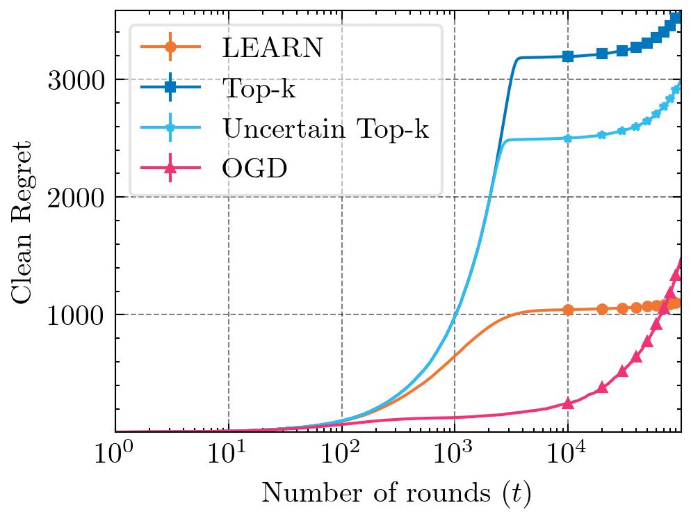
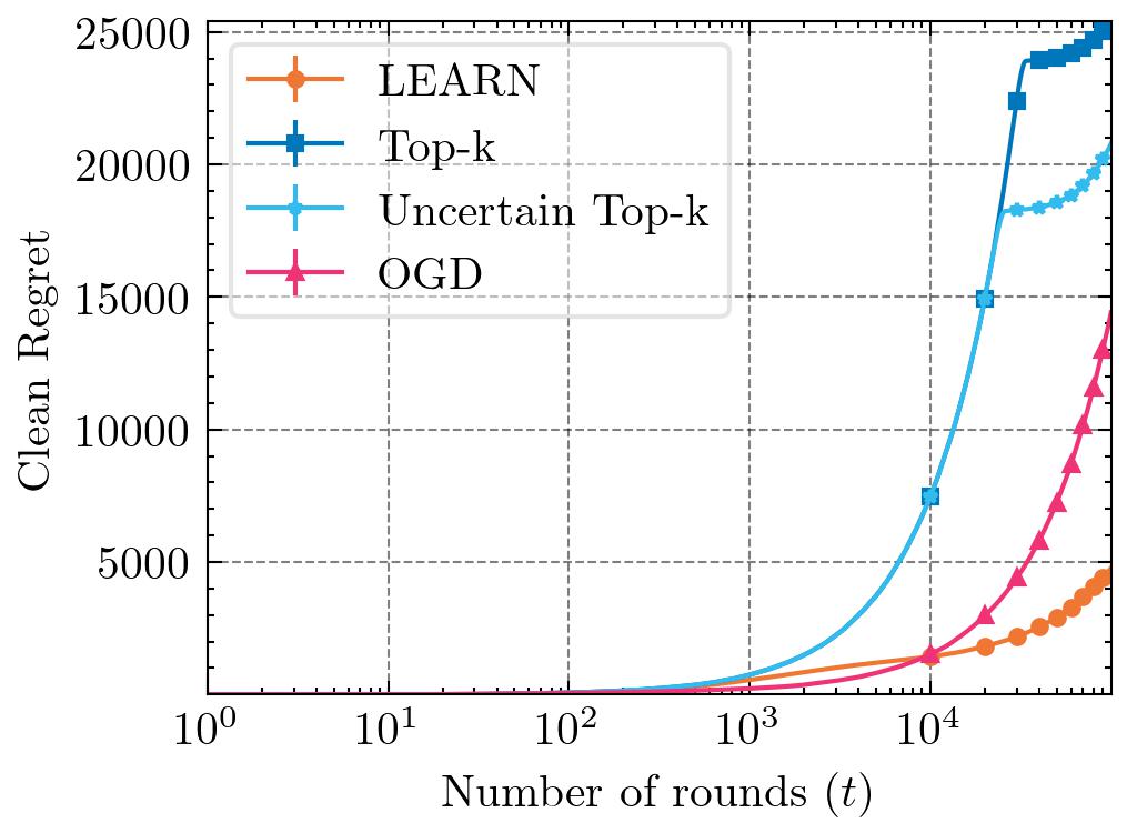
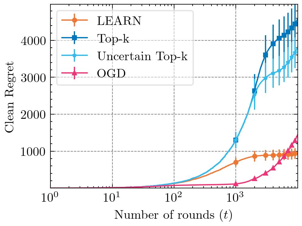
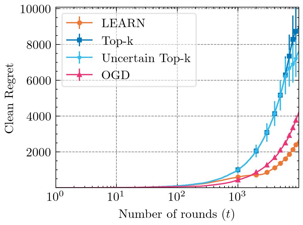
This section presents numerical experiments conducted to substantiate our theoretical findings. We focus on two quintessential machine learning problems, online linear regression, and classification to validate our theory. In particular, we focus on online ridge regression and online support vector machine (SVM). We compare Learn with the Top-k filter algorithm (Top-k) ofย van Erven etย al., (2021) and vanilla online gradient descent (OGD). Note that Top-k has access to the number of outliers $k$, but Learn does not know $k$. We also implemented an uncertain version of Top-k, labeled โ€œUncertain Top-kโ€, which only has access to an estimate of $k$ fixed at $0.75k$. We conduct experiments in an unbounded domain with potentially large gradients of $m$-strongly convex loss functions. Note that none of the baselines provide theoretical guarantees for unbounded domains with outliers. All methods employ the same stepsize $\alpha=\frac{1}{\sqrt{T}}$. We would like to clarify our choice of step size in the experiments. Given that the losses are $m$-strongly convex, it is possible to set $\alpha_{t}=\frac{1}{mt}$ for the baselines. However, in our experiments, the value of $m$ was very small ($m=\lambda=10^{-}4$), which results in a large step size. Consequently, the expected regret bound of $\mathcal{O}(\frac{\log T}{m})$ becomes quite large. A numerical comparison revealed that using $\alpha=\frac{1}{\sqrt{T}}$ yields smaller regret for the baselines. Therefore, we opted for this more favorable step size in our experimental setup. We report the results for the clean dynamic regrets in Figureย 2, averaged across $30$ independent runs with the standard errors. We provide additional experimental details in Appendixย I.2 and Appendixย I.3.

Refer to caption
(a) $k=0$
Refer to caption
(b) $k=\sqrt{T}$
Refer to caption
(c) $k=T^{\frac{2}{3}}$
Refer to caption
(d) $k=\frac{T}{4}$
Refer to caption
(e) $k=0$
Refer to caption
(f) $k=\sqrt{T}$
Refer to caption
(g) $k=T^{\frac{2}{3}}$
Refer to caption
(h) $k=\frac{T}{4}$
Figure 2: Clean dynamic regret plots for different algorithms running on the Online Ridge Regression (Top row, Figuresย 2(a)-2(d)) and Online SVM (Bottom row, Figuresย 2(e)-2(h)).
Online linear regression

In this experiment, the learner encounters the following loss function $f_{t}$ at each round for a fixed $\lambda=10^{-4}$:

$\displaystyle f_{t}\big{(}(x_{t},y_{t}),\theta\big{)}=\frac{\lambda}{2}\|\theta\|^{2}+(y_{t}-\langle x_{t}\,,\theta\rangle)^{2}~{}.$ (17)

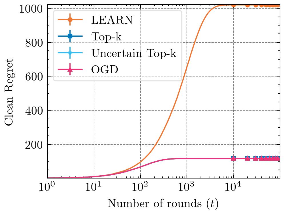
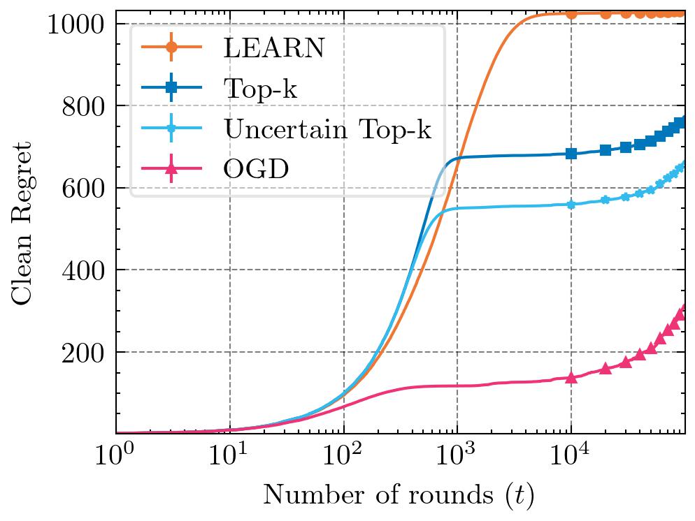
The response for uncorrupted rounds is generated using the linear model $y_{t}=\langle\theta^{*}\,,x_{t}\rangle+e_{t}$ with a unit norm $\theta^{*}\in[-1,1]^{100}$. The entries of $x_{t}$ are drawn independently from the normal distribution $\mathcal{N}(0,1)$. Additionally, the additive noise $e_{t}$ is independently chosen from $\mathcal{N}(0,10^{-6})$. For corrupted rounds, $y_{t}$ is chosen uniformly at random from the interval $[0,1]$. Figuresย 2(a)-2(d) show the results from our experiments with varying numbers of outliers over $T=10^{5}$ rounds.

Online SVM

Following Shalev-Shwartz etย al., (2007), we address the primal version of the online SVM problem. With $\lambda$ set at $10^{-4}$, consistent with Shalev-Shwartz etย al., (2007), the learner faces the following loss in each round $t$:

$\displaystyle f_{t}\big{(}(x_{t},y_{t}),\theta\big{)}=\frac{\lambda}{2}\|\theta\|^{2}+\max(0,1-y_{t}\langle x_{t}\,,\theta\rangle)~{}.$ (18)

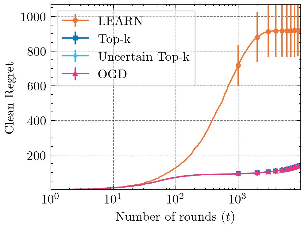
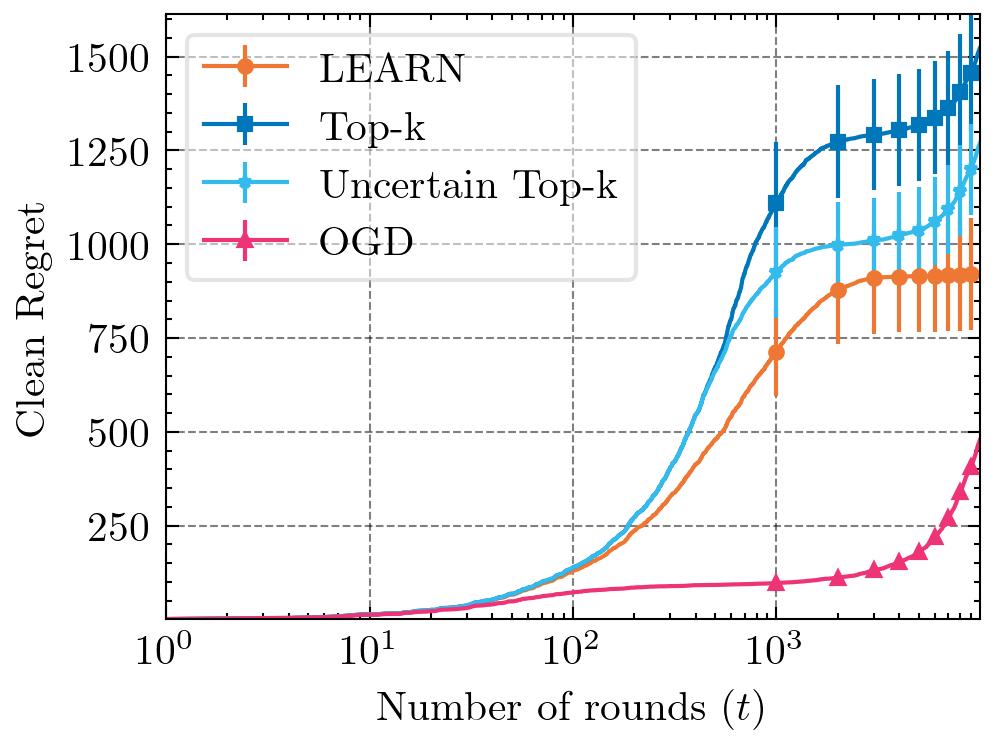
The labels for the uncorrupted rounds are generated according to $y_{t}=\text{sign}\big{(}\langle\theta^{*}\,,x_{t}\rangle\big{)}$, where $\theta^{*}\in[1,11]^{2}$. Mislabeling occurs with probability $0.05$ when $|\langle\theta^{*}\,,x_{t}\rangle|\leq 0.1$. The entries of $x_{t}$ are drawn independently from $\mathcal{N}(0,100)$. For corrupted rounds, the adversary flips the sign of $y_{t}$. Figuresย 2(e)-2(h) show the experimental results with varying numbers of outliers over $T=10^{4}$ rounds.

In the absence of outliers ($k=0$), the results for both online linear regression (Figure 2(a)) and Online SVM (Figureย 2(e)) illustrate a significant gap in the cumulative clean regret of Learn compared to other baselines. Learn is intentionally designed to anticipate outliers in the data, leading to cautious and slow updates initially, resulting in a substantial accumulation of regret in the beginning. However, the regret plot for Learn levels off after the initial few rounds. As the number of outliers increase (Figures 2(b) and 2(c) for online linear regression and Figuresย 2(f) and 2(g) for online SVM), the performance of all methods, except Learn, deteriorates significantly. Although OGD initially incurs small regret, its growth rate is the largest, implying that it will eventually surpass other methods. Learn, on the other hand, maintains roughly the same regret until $k=T^{\frac{2}{3}}$. This demonstrates Learnโ€™s robustness to outliers, even with higher outlier proportions. These observations corroborate our result in equationย (70) of Theorem 3.3, which predicts sublinear behavior for sublinear $k$. Lastly, recall that with $k=\frac{T}{4}$, equationย (70) in Theoremย 3.3 does not assure sublinear regret. Correspondingly, Learn and other methods exhibit increasing regrets in this regime.

5 Conclusion and future work

In this work, we established tight dynamic regret guarantees within the robust OCO framework. Introducing the Learn algorithm, we showcased its effectiveness in handling outliers even when the outlier count $k$ remained unknown, particularly when the loss functions are $m$-strongly convex. Moreover, our algorithm worked with unbounded domains and accommodated large gradients. Central to our algorithm, we employ Learn loss $g$, an invex robust loss designed to diminish the influence of outliers during gradient descent style updates. Additionally, we formulated a unified analysis framework to develop online optimization algorithms tailored for a class of non-convex losses referred to as invex losses. This framework serves as the basis for obtaining regret bounds associated with the Learn loss. To substantiate our theoretical findings, we also conducted numerical experiments. A few natural extensions of our work include studying the robust loss $g_{t}$ with dynamic parameters $a_{t}$ and $b_{t}$ and leveraging the unified analysis framework to develop novel algorithms for various invex losses. In future, exploring the application of invex losses in online learning beyond the context of handling outliers would be interesting.

References

  • Barron, (2019) Barron, J.ย T. (2019). A general and adaptive robust loss function. In Proceedings of the IEEE/CVF Conference on Computer Vision and Pattern Recognition, pages 4331โ€“4339.
  • Beaton and Tukey, (1974) Beaton, A.ย E. and Tukey, J.ย W. (1974). The fitting of power series, meaning polynomials, illustrated on band-spectroscopic data. Technometrics, 16(2):147โ€“185.
  • Belagiannis etย al., (2015) Belagiannis, V., Rupprecht, C., Carneiro, G., and Navab, N. (2015). Robust optimization for deep regression. In 2015 IEEE International Conference on Computer Vision (ICCV). IEEE.
  • Bhaskara and Ruwanpathirana, (2020) Bhaskara, A. and Ruwanpathirana, A.ย K. (2020). Robust algorithms for online $k$-means clustering. In Proceedings of the 31st International Conference on Algorithmic Learning Theory, volume 117 of Proceedings of Machine Learning Research, pages 148โ€“173. PMLR.
  • Black and Anandan, (1996) Black, M.ย J. and Anandan, P. (1996). The robust estimation of multiple motions: Parametric and piecewise-smooth flow fields. Computer Vision and Image Understanding, 63(1):75โ€“104.
  • Chang etย al., (2018) Chang, L., Roberts, S., and Welsh, A. (2018). Robust lasso regression using tukeyโ€™s biweight criterion. Technometrics, 60(1):36โ€“47.
  • Chen etย al., (2022) Chen, S., Koehler, F., Moitra, A., and Yau, M. (2022). Online and distribution-free robustness: Regression and contextual bandits with huber contamination. In 2021 IEEE 62nd Annual Symposium on Foundations of Computer Science (FOCS), pages 684โ€“695. IEEE.
  • D.ย Hendricks and Wilcox, (2016) D.ย Hendricks, T.ย G. and Wilcox, D. (2016). Detecting intraday financial market states using temporal clustering. Quantitative Finance, 16(11):1657โ€“1678.
  • Dennis and Welsch, (1978) Dennis, J.ย E. and Welsch, R.ย E. (1978). Techniques for nonlinear least squares and robust regression. Communications in Statistics - Simulation and Computation, 7:345โ€“359.
  • Diakonikolas and Kane, (2023) Diakonikolas, I. and Kane, D.ย M. (2023). Algorithmic high-dimensional robust statistics. Cambridge university press.
  • Diakonikolas etย al., (2022) Diakonikolas, I., Kane, D.ย M., Pensia, A., and Pittas, T. (2022). Streaming algorithms for high-dimensional robust statistics. In International Conference on Machine Learning, pages 5061โ€“5117. PMLR.
  • Fedoryszak etย al., (2019) Fedoryszak, M., Frederick, B., Rajaram, V., and Zhong, C. (2019). Real-time event detection on social data streams. In Proceedings of the 25th ACM SIGKDD International Conference on Knowledge Discovery & Data Mining, KDD โ€™19, page 2774โ€“2782, New York, NY, USA. Association for Computing Machinery.
  • Feng etย al., (2017) Feng, J., Xu, H., and Mannor, S. (2017). Outlier robust online learning. arXiv preprint arXiv:1701.00251.
  • Gokcesu and Gokcesu, (2021) Gokcesu, K. and Gokcesu, H. (2021). Generalized huber loss for robust learning and its efficient minimization for a robust statistics. arXiv preprint arXiv:2108.12627.
  • Hampel etย al., (2011) Hampel, F., Ronchetti, E., Rousseeuw, P., and Stahel, W. (2011). Robust Statistics: The Approach Based on Influence Functions. Wiley Series in Probability and Statistics. Wiley.
  • Hazan, (2023) Hazan, E. (2023). Introduction to online convex optimization.
  • Huber, (1964) Huber, P.ย J. (1964). Robust Estimation of a Location Parameter. The Annals of Mathematical Statistics, 35(1):73 โ€“ 101.
  • Huber, (1973) Huber, P.ย J. (1973). Robust regression: asymptotics, conjectures and monte carlo. The annals of statistics, pages 799โ€“821.
  • Jacobsen and Cutkosky, (2023) Jacobsen, A. and Cutkosky, A. (2023). Unconstrained online learning with unbounded losses. In Proceedings of the 40th International Conference on Machine Learning, volume 202 of Proceedings of Machine Learning Research, pages 14590โ€“14630. PMLR.
  • Kejariwal etย al., (2015) Kejariwal, A., Kulkarni, S., and Ramasamy, K. (2015). Real time analytics: algorithms and systems. Proceedings of the VLDB Endowment, 8(12):2040โ€“2041.
  • Lozano and Meinshausen, (2013) Lozano, A.ย C. and Meinshausen, N. (2013). Minimum distance estimation for robust high-dimensional regression. arXiv preprint arXiv:1307.3227.
  • Maronna etย al., (2006) Maronna, R., Martin, D., and Yohai, V. (2006). Robust Statistics: Theory and Methods. Wiley Series in Probability and Statistics. Wiley.
  • Orabona, (2023) Orabona, F. (2023). A modern introduction to online learning.
  • Shalev-Shwartz etย al., (2007) Shalev-Shwartz, S., Singer, Y., and Srebro, N. (2007). Pegasos: Primal estimated sub-gradient solver for svm. In Proceedings of the 24th International Conference on Machine learning, pages 807โ€“814.
  • van Erven etย al., (2021) van Erven, T., Sachs, S., Koolen, W.ย M., and Kotlowski, W. (2021). Robust online convex optimization in the presence of outliers. In Conference on Learning Theory, pages 4174โ€“4194. PMLR.
  • Wang etย al., (2023) Wang, X., Tu, Z., Hong, Y., Wu, Y., and Shi, G. (2023). Online optimization over riemannian manifolds. Journal of Machine Learning Research, 24(84):1โ€“67.
  • Zhang etย al., (2015) Zhang, F., Cao, J., Khan, S.ย U., Li, K., and Hwang, K. (2015). A task-level adaptive mapreduce framework for real-time streaming data in healthcare applications. Future Generation Computer Systems, 43-44:149โ€“160.
  • Zhang etย al., (2018) Zhang, L., Lu, S., and Zhou, Z.-H. (2018). Adaptive online learning in dynamic environments. In Proceedings of the 32nd International Conference on Neural Information Processing Systems, NIPSโ€™18, page 1330โ€“1340, Red Hook, NY, USA. Curran Associates Inc.
  • Zhang etย al., (2017) Zhang, L., Yang, T., Yi, J., Jin, R., and Zhou, Z.-H. (2017). Improved dynamic regret for non-degenerate functions. Advances in Neural Information Processing Systems, 30.

Appendix A Related Work

This section provides a detailed overview of closely related lines of research that inform our work.

Outlier Robust Online Learning

Our work builds on the work of ย van Erven etย al., (2021) where they consider the OCO framework when outliers are present. They specifically address the scenario where $k$, the number of outliers, is known in advance, and the adversary can arbitrarily corrupt any of the $k$ rounds. The model assumes that inliers have a bounded range (not known), while outliers can extend to an unbounded range. Notably, learner performance is quantified through clean static regret. The core of their algorithm involves the maintaining of top-$k$ gradients, triggering updates to the online learning algorithm only when the norm of the gradient is less than 2 times the minimum norm within the top-$k$ gradients. They establish robust regret guarantees, offering $\mathcal{O}(G(\mathcal{S})(\sqrt{T}+k))$ for convex functions and $\mathcal{O}(\log T+G(\mathcal{S})k)$ for strongly convex functions, where $G(\mathcal{S})$ represents the norm of the largest gradient considering only clean rounds. Their work, while providing valuable insights, assumes known values for $k$, a bounded domain, and the existence of a Lipschitz bound $G(\mathcal{S})$ for clean rounds. In contrast, our work extends beyond these assumptions, particularly focusing on dynamic environments where the number of outliers is unknown, the domain is unbounded, and the losses may not be Lipschitz.

Robust Losses

A pivotal element of our investigation lies in formulating and examining a non-convex robust loss function. To contextualize our work, we highlight pertinent robust losses featured in the existing literature. Notable examples include Huber lossย (Huber,, 1964), Tukeyโ€™s biweight lossย (Beaton and Tukey,, 1974), Welsch lossย (Dennis and Welsch,, 1978) and Cauchy lossย (Black and Anandan,, 1996) among others, each tailored to address different applications. Huber loss, for instance, strikes a balance between mean squared error and mean absolute error, rendering it suitable for robust regressionย (Huber,, 1973). Similarly, Tukeyโ€™s biweight loss, known for its efficacy in robust regression, provides resistance against outliers through a truncated quadratic penaltyย (Chang etย al.,, 2018). It is worth noting that Tukeyโ€™s biweight loss, along with Cauchy and Welsch losses, are non-convex and satisfy the redescending propertyย (Hampel etย al.,, 2011). Learn loss also shares this attribute. For a detailed comparison of Learn loss with different robust losses see Appendixย C. Various generalizations and extensions of these losses have been studied ย (Barron,, 2019; Gokcesu and Gokcesu,, 2021), reflecting the extensive exploration and adaptation of robust loss functions within the broader literature.

OCO with unbounded domains and gradients

It was only in the recent work ofย Jacobsen and Cutkosky, (2023) that a sublinear regret guarantee was achieved by avoiding the assumption that there exists $\|\nabla f_{t}\|\leq G$ for all rounds $t$. They obtain sublinear regret guarantees in the standard OCO framework when the domain is unbounded, and the gradients grow large with the norm of actions ($\|\theta_{t}\|$). They provide the first algorithm for dynamic regret minimization in the unbounded domain and gradient setup. In this work, we adopt an expert scheme akin to theirs to handle unbounded domains and gradients that can grow large in the robust outlier framework.

Related Applications

The work ofย Chen etย al., (2022) studies online linear regression within a realizable context, accounting for small noise using the Huber contamination modelย (Huber,, 1964). However, our model (similarly the model ofย van Erven etย al., (2021)) differs from theirs significantly. Notably, we do not impose any assumptions of realizability or control the corruption mechanism through probabilistic assumptions. Although distinct in the techniques employed, it is important to acknowledge a substantial body of related work addressing robust optimization in various theoretical computer science and machine learning problems. For a comprehensive overview, the textbook authored by Diakonikolas and Kane, (2023) stands out as an excellent reference.

Appendix B Dynamic Regret in a Bounded Domain Using Top-k Filter Algorithm

van Erven etย al., (2021) established a tight bound on static regret within a bounded domain, assuming prior knowledge of $k$. For convex losses, they achieved an optimal static regret upper bound of $\mathcal{O}(\sqrt{T}+k)$. In the case of strongly convex losses, this bound is further improved to $\mathcal{O}(\log T+k)$, which remains optimal. In this section, we extend their results to the dynamic setting and establish a clean dynamic regret bound of $\mathcal{O}(\sqrt{V_{T}T}+k)$ within a bounded domain. Notably, this bound remains tight even for strongly convex functionsย (Zhang etย al.,, 2017).

We make the following assumptions for our extension:

  1. 1.

    The Lipschitz-adaptive algorithm ALG used byย van Erven etย al., (2021) is online gradient descent (OGD).

  2. 2.

    The domain $\Theta$ is bounded.

Let $\mathcal{S}\subseteq[T]$ be the set of uncorrupted rounds. Then, we are interested in bounding the clean dynamic regret defined as:

โ„œRโ€‹DTโ€‹(ฮธ,๐’ฎ)=โˆ‘tโˆˆ๐’ฎ(ftโ€‹(st,ฮธt)โˆ’ftโ€‹(st,ฮธtโˆ—)),superscriptsubscriptโ„œ๐‘…๐ท๐‘‡๐œƒ๐’ฎsubscript๐‘ก๐’ฎsubscript๐‘“๐‘กsubscript๐‘ ๐‘กsubscript๐œƒ๐‘กsubscript๐‘“๐‘กsubscript๐‘ ๐‘กsuperscriptsubscript๐œƒ๐‘ก\displaystyle\mathfrak{R}_{RD}^{T}(\mathbf{\theta},\mathcal{S})=\sum_{t\in\mathcal{S}}\Big{(}f_{t}(s_{t},\theta_{t})-f_{t}(s_{t},\theta_{t}^{*})\Big{)}~{}, (19)

Let $\mathcal{F}\subset[T]$ denote the rounds flitered out by Algorithm 1 in van Erven etย al., (2021), and let $\mathcal{P}=[T]\setminus\mathcal{F}$ denote the rounds that are passed on to ALG. Then,

โ„œRโ€‹DTโ€‹(ฮธ,๐’ฎ)=โˆ‘tโˆˆ๐’ฎโˆฉ๐’ซ(ftโ€‹(st,ฮธt)โˆ’ftโ€‹(st,ฮธtโˆ—))โŸT1+โˆ‘tโˆˆ๐’ฎโˆฉโ„ฑ(ftโ€‹(st,ฮธt)โˆ’ftโ€‹(st,ฮธtโˆ—))โŸT2superscriptsubscriptโ„œ๐‘…๐ท๐‘‡๐œƒ๐’ฎsubscriptโŸsubscript๐‘ก๐’ฎ๐’ซsubscript๐‘“๐‘กsubscript๐‘ ๐‘กsubscript๐œƒ๐‘กsubscript๐‘“๐‘กsubscript๐‘ ๐‘กsuperscriptsubscript๐œƒ๐‘กsubscript๐‘‡1subscriptโŸsubscript๐‘ก๐’ฎโ„ฑsubscript๐‘“๐‘กsubscript๐‘ ๐‘กsubscript๐œƒ๐‘กsubscript๐‘“๐‘กsubscript๐‘ ๐‘กsuperscriptsubscript๐œƒ๐‘กsubscript๐‘‡2\displaystyle\mathfrak{R}_{RD}^{T}(\mathbf{\theta},\mathcal{S})=\underbrace{\sum_{t\in\mathcal{S}\cap\mathcal{P}}\Big{(}f_{t}(s_{t},\theta_{t})-f_{t}(s_{t},\theta_{t}^{*})\Big{)}}_{T_{1}}+\underbrace{\sum_{t\in\mathcal{S}\cap\mathcal{F}}\Big{(}f_{t}(s_{t},\theta_{t})-f_{t}(s_{t},\theta_{t}^{*})\Big{)}}_{T_{2}} (20)

First, we bound $T_{1}$.

T1=โˆ‘tโˆˆ๐’ซ(ftโ€‹(st,ฮธt)โˆ’ftโ€‹(st,ฮธtโˆ—))โŸT11โˆ’โˆ‘tโˆˆ๐’ซโˆ–๐’ฎ(ftโ€‹(st,ฮธt)โˆ’ftโ€‹(st,ฮธtโˆ—))โŸT12subscript๐‘‡1subscriptโŸsubscript๐‘ก๐’ซsubscript๐‘“๐‘กsubscript๐‘ ๐‘กsubscript๐œƒ๐‘กsubscript๐‘“๐‘กsubscript๐‘ ๐‘กsuperscriptsubscript๐œƒ๐‘กsubscript๐‘‡11subscriptโŸsubscript๐‘ก๐’ซ๐’ฎsubscript๐‘“๐‘กsubscript๐‘ ๐‘กsubscript๐œƒ๐‘กsubscript๐‘“๐‘กsubscript๐‘ ๐‘กsuperscriptsubscript๐œƒ๐‘กsubscript๐‘‡12\displaystyle T_{1}=\underbrace{\sum_{t\in\mathcal{P}}\Big{(}f_{t}(s_{t},\theta_{t})-f_{t}(s_{t},\theta_{t}^{*})\Big{)}}_{T_{11}}-\underbrace{\sum_{t\in\mathcal{P}\setminus\mathcal{S}}\Big{(}f_{t}(s_{t},\theta_{t})-f_{t}(s_{t},\theta_{t}^{*})\Big{)}}_{T_{12}} (21)

The bound for the term $T_{12}$ follows directly from van Erven etย al., (2021)โ€™s proof of their Theorem 1:

T12โ‰คโˆ‘tโˆˆ๐’ซโˆ–๐’ฎโˆ‡ftโ€‹(st,ฮธt)Tโ€‹(ฮธtโˆ’ฮธtโˆ—)โ‰ค2โ€‹Dโ€‹Gโ€‹(๐’ฎ)โ€‹k,subscript๐‘‡12subscript๐‘ก๐’ซ๐’ฎโˆ‡subscript๐‘“๐‘กsuperscriptsubscript๐‘ ๐‘กsubscript๐œƒ๐‘ก๐‘‡subscript๐œƒ๐‘กsuperscriptsubscript๐œƒ๐‘ก2๐ท๐บ๐’ฎ๐‘˜\displaystyle T_{12}\leq\sum_{t\in\mathcal{P}\setminus\mathcal{S}}\nabla f_{t}(s_{t},\theta_{t})^{T}(\theta_{t}-\theta_{t}^{*})\leq 2DG(\mathcal{S})k~{}, (22)

where $D=\max_{a,b\in\Theta}\|a-b\|$ and Gโ€‹(๐’ฎ)=maxtโˆˆ๐’ฎโกโ€–โˆ‡ftโ€‹(st,ฮธt)โ€–๐บ๐’ฎsubscript๐‘ก๐’ฎnormโˆ‡subscript๐‘“๐‘กsubscript๐‘ ๐‘กsubscript๐œƒ๐‘กG(\mathcal{S})=\max_{t\in\mathcal{S}}\|\nabla f_{t}(s_{t},\theta_{t})\|.

Similarly, we take the bound for $T_{2}$ directly from van Erven etย al., (2021)โ€™s proof of Theorem 1:

T2โ‰คโˆ‘tโˆˆ๐’ฎโˆฉโ„ฑโˆ‡ftโ€‹(st,ฮธt)Tโ€‹(ฮธtโˆ’ฮธtโˆ—)โ‰ค2โ€‹Dโ€‹Gโ€‹(๐’ฎ)โ€‹(k+1)subscript๐‘‡2subscript๐‘ก๐’ฎโ„ฑโˆ‡subscript๐‘“๐‘กsuperscriptsubscript๐‘ ๐‘กsubscript๐œƒ๐‘ก๐‘‡subscript๐œƒ๐‘กsuperscriptsubscript๐œƒ๐‘ก2๐ท๐บ๐’ฎ๐‘˜1\displaystyle T_{2}\leq\sum_{t\in\mathcal{S}\cap\mathcal{F}}\nabla f_{t}(s_{t},\theta_{t})^{T}(\theta_{t}-\theta_{t}^{*})\leq 2DG(\mathcal{S})(k+1) (23)

At this point, it only remains to bound $T_{11}$. Recall that OGD (instantiation of ALG) only sees the rounds in $\mathcal{P}$, and by reindexing them as $t\in\{1,\ldots,|\mathcal{P}|\}$, we can write for all $t\in[|\mathcal{P}|]$:

$\displaystyle\|\theta_{t+1}-\theta_{t+1}^{*}\|^{2}=\|\theta_{t+1}-\theta_{t}^{*}+\theta_{t}^{*}-\theta_{t+1}^{*}\|^{2}$ (24)

Expanding RHS and by definition of $D$, we have:

$\displaystyle\|\theta_{t+1}-\theta_{t+1}^{*}\|^{2}\leq\|\theta_{t+1}-\theta_{t}^{*}\|^{2}+3D\|\theta_{t}^{*}-\theta_{t+1}^{*}\|$ (25)

Now, substituting ฮธt+1=ฮ ฮธโˆˆฮ˜โ€‹(ฮธtโˆ’ฮฑtโ€‹โˆ‡ftโ€‹(st,ฮธt))subscript๐œƒ๐‘ก1subscriptฮ ๐œƒฮ˜subscript๐œƒ๐‘กsubscript๐›ผ๐‘กโˆ‡subscript๐‘“๐‘กsubscript๐‘ ๐‘กsubscript๐œƒ๐‘ก\theta_{t+1}=\Pi_{\theta\in\Theta}\Big{(}\theta_{t}-\alpha_{t}\nabla f_{t}(s_{t},\theta_{t})\Big{)} and using the contractive property of the projection on a convex set, we can write:

โ€–ฮธt+1โˆ’ฮธt+1โˆ—โ€–2โ‰คโ€–ฮธtโˆ’ฮฑtโ€‹โˆ‡ftโ€‹(st,ฮธt)โˆ’ฮธtโˆ—โ€–2+3โ€‹Dโ€‹โ€–ฮธtโˆ—โˆ’ฮธt+1โˆ—โ€–superscriptnormsubscript๐œƒ๐‘ก1superscriptsubscript๐œƒ๐‘ก12superscriptnormsubscript๐œƒ๐‘กsubscript๐›ผ๐‘กโˆ‡subscript๐‘“๐‘กsubscript๐‘ ๐‘กsubscript๐œƒ๐‘กsuperscriptsubscript๐œƒ๐‘ก23๐ทnormsuperscriptsubscript๐œƒ๐‘กsuperscriptsubscript๐œƒ๐‘ก1\displaystyle\|\theta_{t+1}-\theta_{t+1}^{*}\|^{2}\leq\|\theta_{t}-\alpha_{t}\nabla f_{t}(s_{t},\theta_{t})-\theta_{t}^{*}\|^{2}+3D\|\theta_{t}^{*}-\theta_{t+1}^{*}\| (26)

Simplifying,

โ€–ฮธt+1โˆ’ฮธt+1โˆ—โ€–2โ‰คโ€–ฮธtโˆ’ฮธtโˆ—โ€–2+ฮฑt2โ€‹โ€–โˆ‡ftโ€‹(st,ฮธt)โ€–2โˆ’2โ€‹ฮฑtโ€‹โˆ‡ftโ€‹(st,ฮธt)Tโ€‹(ฮธtโˆ’ฮธtโˆ—)+3โ€‹Dโ€‹โ€–ฮธtโˆ—โˆ’ฮธt+1โˆ—โ€–superscriptnormsubscript๐œƒ๐‘ก1superscriptsubscript๐œƒ๐‘ก12superscriptnormsubscript๐œƒ๐‘กsuperscriptsubscript๐œƒ๐‘ก2superscriptsubscript๐›ผ๐‘ก2superscriptnormโˆ‡subscript๐‘“๐‘กsubscript๐‘ ๐‘กsubscript๐œƒ๐‘ก22subscript๐›ผ๐‘กโˆ‡subscript๐‘“๐‘กsuperscriptsubscript๐‘ ๐‘กsubscript๐œƒ๐‘ก๐‘‡subscript๐œƒ๐‘กsuperscriptsubscript๐œƒ๐‘ก3๐ทnormsuperscriptsubscript๐œƒ๐‘กsuperscriptsubscript๐œƒ๐‘ก1\displaystyle\|\theta_{t+1}-\theta_{t+1}^{*}\|^{2}\leq\|\theta_{t}-\theta_{t}^{*}\|^{2}+\alpha_{t}^{2}\|\nabla f_{t}(s_{t},\theta_{t})\|^{2}-2\alpha_{t}\nabla f_{t}(s_{t},\theta_{t})^{T}(\theta_{t}-\theta_{t}^{*})+3D\|\theta_{t}^{*}-\theta_{t+1}^{*}\| (27)

Taking $\alpha_{t}=\alpha>0$ and using the convexity of ftโ€‹(st,ฮธt)subscript๐‘“๐‘กsubscript๐‘ ๐‘กsubscript๐œƒ๐‘กf_{t}(s_{t},\theta_{t}), we get:

2โ€‹ฮฑโ€‹(ftโ€‹(st,ฮธt)โˆ’ftโ€‹(st,ฮธtโˆ—))โ‰คโ€–ฮธtโˆ’ฮธtโˆ—โ€–2โˆ’โ€–ฮธt+1โˆ’ฮธt+1โˆ—โ€–2+ฮฑ2โ€‹โ€–โˆ‡ftโ€‹(st,ฮธt)โ€–2+3โ€‹Dโ€‹โ€–ฮธtโˆ—โˆ’ฮธt+1โˆ—โ€–2๐›ผsubscript๐‘“๐‘กsubscript๐‘ ๐‘กsubscript๐œƒ๐‘กsubscript๐‘“๐‘กsubscript๐‘ ๐‘กsuperscriptsubscript๐œƒ๐‘กsuperscriptnormsubscript๐œƒ๐‘กsuperscriptsubscript๐œƒ๐‘ก2superscriptnormsubscript๐œƒ๐‘ก1superscriptsubscript๐œƒ๐‘ก12superscript๐›ผ2superscriptnormโˆ‡subscript๐‘“๐‘กsubscript๐‘ ๐‘กsubscript๐œƒ๐‘ก23๐ทnormsuperscriptsubscript๐œƒ๐‘กsuperscriptsubscript๐œƒ๐‘ก1\displaystyle 2\alpha\Big{(}f_{t}(s_{t},\theta_{t})-f_{t}(s_{t},\theta_{t}^{*})\Big{)}\leq\|\theta_{t}-\theta_{t}^{*}\|^{2}-\|\theta_{t+1}-\theta_{t+1}^{*}\|^{2}+\alpha^{2}\|\nabla f_{t}(s_{t},\theta_{t})\|^{2}+3D\|\theta_{t}^{*}-\theta_{t+1}^{*}\| (28)

Summing it across all $t\in[|\mathcal{P}|]$:

T11โ‰คโ€–ฮธ1โˆ’ฮธ1โˆ—โ€–22โ€‹ฮฑ+ฮฑ2โ€‹โˆ‘tโˆˆ๐’ซโ€–โˆ‡ftโ€‹(st,ฮธt)โ€–2+3โ€‹D2โ€‹ฮฑโ€‹โˆ‘tโˆˆ๐’ซโ€–ฮธtโˆ—โˆ’ฮธt+1โˆ—โ€–subscript๐‘‡11superscriptnormsubscript๐œƒ1superscriptsubscript๐œƒ122๐›ผ๐›ผ2subscript๐‘ก๐’ซsuperscriptnormโˆ‡subscript๐‘“๐‘กsubscript๐‘ ๐‘กsubscript๐œƒ๐‘ก23๐ท2๐›ผsubscript๐‘ก๐’ซnormsuperscriptsubscript๐œƒ๐‘กsuperscriptsubscript๐œƒ๐‘ก1\displaystyle T_{11}\leq\frac{\|\theta_{1}-\theta_{1}^{*}\|^{2}}{2\alpha}+\frac{\alpha}{2}\sum_{t\in\mathcal{P}}\|\nabla f_{t}(s_{t},\theta_{t})\|^{2}+\frac{3D}{2\alpha}\sum_{t\in\mathcal{P}}\|\theta_{t}^{*}-\theta_{t+1}^{*}\| (29)

We make two observations:

  1. 1.

    โ€–โˆ‡ftโ€‹(st,ฮธt)โ€–โ‰ค2โ€‹Gโ€‹(๐’ฎ),โˆ€tโˆˆ๐’ซformulae-sequencenormโˆ‡subscript๐‘“๐‘กsubscript๐‘ ๐‘กsubscript๐œƒ๐‘ก2๐บ๐’ฎfor-all๐‘ก๐’ซ\|\nabla f_{t}(s_{t},\theta_{t})\|\leq 2G(\mathcal{S}),\forall t\in\mathcal{P} - due to van Erven etย al., (2021)

  2. 2.

    $\sum_{t\in\mathcal{P}}\|\theta_{t}^{*}-\theta_{t+1}^{*}\|\leq\sum_{t\in[T]}\|\theta_{t}^{*}-\theta_{t+1}^{*}\|=V_{T}$

We choose $\alpha=\frac{\sqrt{3DV_{T}+D^{2}}}{2G(\mathcal{S})\sqrt{T}}$ to get:

$\displaystyle T_{11}\leq 2\sqrt{(3DV_{T}+D^{2})T}G(\mathcal{S})~{}.$ (30)

Combining all the above results together, we get

$\displaystyle\mathfrak{R}_{RD}^{T}(\mathbf{\theta},\mathcal{S})\leq 2\sqrt{(3DV_{T}+D^{2})T}G(\mathcal{S})+2DG(\mathcal{S})k+2DG(\mathcal{S})(k+1)=\mathcal{O}(\sqrt{V_{T}T}+k)~{}.$ (31)

Appendix C Comparison of Robust Losses

Refer to caption
Figure 3: The robust loss closely follows the square loss and flattens out as we move away from the minima.

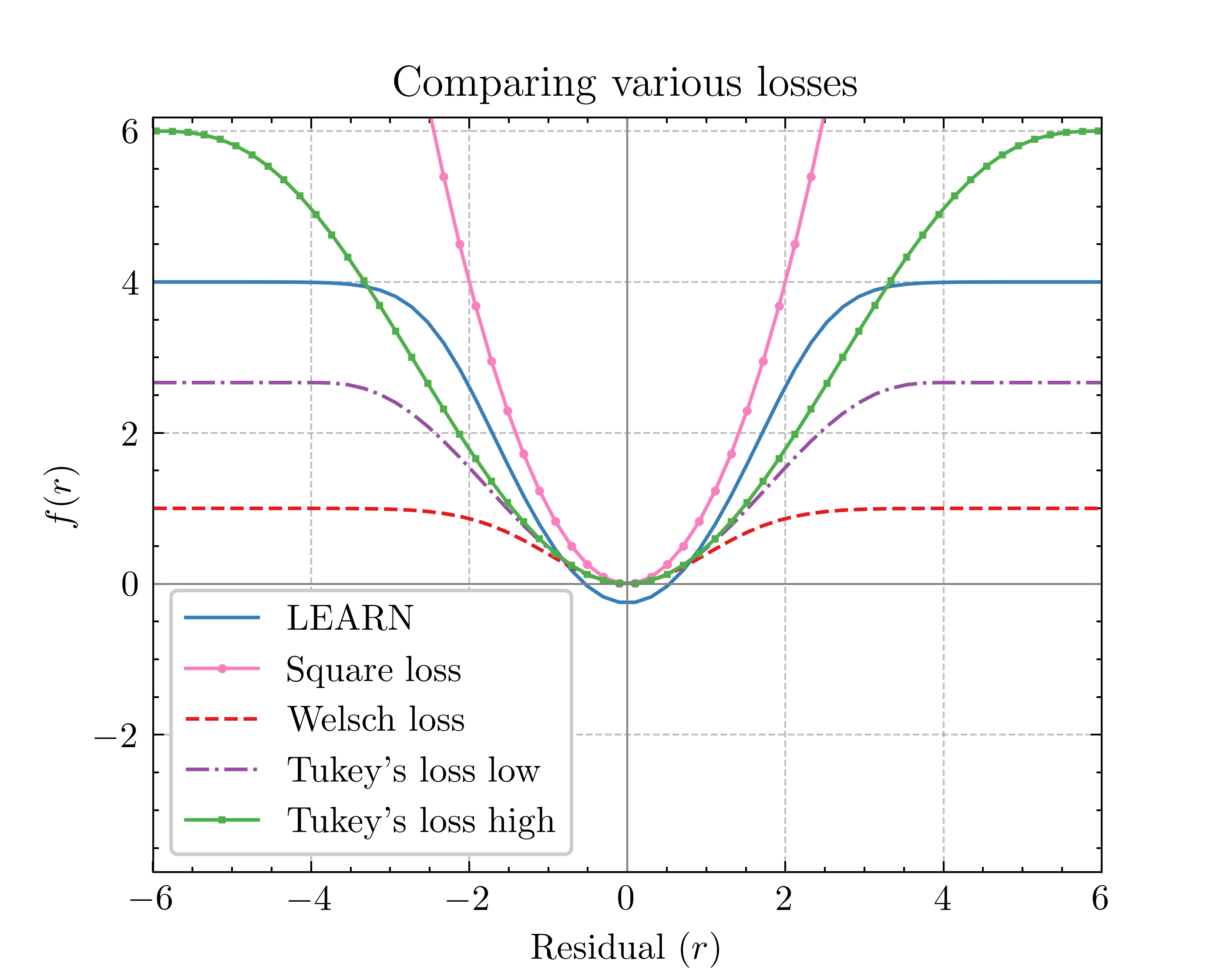
To understand how the robust loss works to mitigate its susceptibility to outliers, we examine the behavior of different non-convex losses, including our robust loss. We compare how these losses resemble the square loss $f$ near the origin and observe their behavior as we deviate from it.

Let us consider the square loss function $f(r)=r^{2}$ where $r$ denotes the residual, and the minimum is attained at 00. Our robust loss, denoted by $g$, instantiated with $f(r)$ with constants $a=2$ and $b=e^{-2}$, is represented in the Figureย 3. Note that $g$ closely follows the behavior of the function $f$ in the vicinity of the origin and gradually levels off as we move away from it. Importantly, the minimizers for both $g$ and $f$ are the same.

In Figureย 3, we plot two other non-convex losses that are similar in appearance to our robust loss. First, we examine Tukeyโ€™s biweight loss, defined as

$\displaystyle\ell(r)=\left\{\begin{array}[]{ll}\frac{c^{2}}{6}\left(1-\left[1-\left(\frac{r}{c}\right)^{2}\right]^{3}\right)&\text{ if }|r|\leq c\\ \frac{c^{2}}{6}&\text{ otherwise }\end{array}\right.$ (34)

where $r$ denotes the residual and $c$ is a tunable parameter. We observe that, even when tuning the parameter $c$ to both high$(c=6)$ and low$(c=4)$ values, the curve fails to closely follow the curvature of the square loss, contrasting with the behavior of our robust loss. Moving away from the origin, Tukeyโ€™s loss flattens out at a slower when compared to $g$.

Next, we consider the Welsch loss defined as

$\displaystyle h(r)=1-\exp\left(-\frac{1}{2}\left(\frac{r}{c}\right)^{2}\right)$ (35)

Here, the tunable parameter is set to $c=2$ in Figureย 3. However, its limitation of being capped at one impedes its ability to track the underlying square loss precisely. This causes it to flatten out early, making it less suitable for online learning. These observations shed light on the distinctive characteristics of these losses and underscore the efficacy of our proposed robust loss in capturing the desired behavior.

Appendix D Invexity of the Robust Loss

D.1 Proof of Lemmaย 3.1

Proof.

To prove that $g_{t}$ is a $\zeta_{t}$-invex function, it suffices to show that all its stationary points are the global minima. Using the monocity of $\log(\cdot)$ and $\exp(\cdot)$ functions, it follows that

ฮธยฏtโˆˆargโกminฮธโˆˆdโกftโ€‹(st,ฮธ)=argโกminฮธโˆˆdโกgtโ€‹(st,ฮธ)subscriptยฏ๐œƒ๐‘กsubscriptsuperscript๐‘‘๐œƒabsentsubscript๐‘“๐‘กsubscript๐‘ ๐‘ก๐œƒsubscriptsuperscript๐‘‘๐œƒabsentsubscript๐‘”๐‘กsubscript๐‘ ๐‘ก๐œƒ\displaystyle\overline{\theta}_{t}\in\arg\min_{\theta\in^{d}}f_{t}(s_{t},\theta)=\arg\min_{\theta\in^{d}}g_{t}(s_{t},\theta) (36)

Due to the convexity of $f_{t}$, either $\nabla f_{t}(\overline{\theta})=0$ or $f_{t}$ does not have any stationary point. Now,

โˆ‡gtโ€‹(ฮธ)=expโก(โˆ’1aโ€‹ftโ€‹(st,ฮธ))b+expโก(โˆ’1aโ€‹ftโ€‹(st,ฮธ))โ€‹โˆ‡ftโ€‹(ฮธ)โˆ‡subscript๐‘”๐‘ก๐œƒ1๐‘Žsubscript๐‘“๐‘กsubscript๐‘ ๐‘ก๐œƒ๐‘1๐‘Žsubscript๐‘“๐‘กsubscript๐‘ ๐‘ก๐œƒโˆ‡subscript๐‘“๐‘ก๐œƒ\displaystyle\nabla g_{t}(\theta)=\frac{\exp(-\frac{1}{a}f_{t}(s_{t},\theta))}{b+\exp(-\frac{1}{a}f_{t}(s_{t},\theta))}\nabla f_{t}(\theta) (37)

It is obvious that $\nabla g_{t}(\theta)=0$ if and only if $\nabla f_{t}(\theta)=0$. This immediately implies that $g_{t}$ is invex. Equivalently, there exists a function $\zeta_{t}(\vartheta_{2},\vartheta_{1})$ such that

gtโ€‹(st,ฯ‘2)โ‰ฅgtโ€‹(st,ฯ‘1)+โŸจโˆ‡gtโ€‹(st,ฯ‘1),ฮถtโ€‹(ฯ‘2,ฯ‘1)โŸฉ.subscript๐‘”๐‘กsubscript๐‘ ๐‘กsubscriptitalic-ฯ‘2subscript๐‘”๐‘กsubscript๐‘ ๐‘กsubscriptitalic-ฯ‘1โˆ‡subscript๐‘”๐‘กsubscript๐‘ ๐‘กsubscriptitalic-ฯ‘1subscript๐œ๐‘กsubscriptitalic-ฯ‘2subscriptitalic-ฯ‘1\displaystyle g_{t}(s_{t},\vartheta_{2})\geq g_{t}(s_{t},\vartheta_{1})+\langle\nabla g_{t}(s_{t},\vartheta_{1})\,,\zeta_{t}(\vartheta_{2},\vartheta_{1})\rangle~{}. (38)

Again, employing the monocity of $\log(\cdot)$ and $\exp(\cdot)$ functions,

ฯ‰tโˆ—โ‰”argโกminฮธโˆˆฮ˜โกftโ€‹(st,ฮธ)=argโกminฮธโˆˆฮ˜โกgtโ€‹(st,ฮธ)โ‰”superscriptsubscript๐œ”๐‘กsubscript๐œƒฮ˜subscript๐‘“๐‘กsubscript๐‘ ๐‘ก๐œƒsubscript๐œƒฮ˜subscript๐‘”๐‘กsubscript๐‘ ๐‘ก๐œƒ\displaystyle\omega_{t}^{*}\coloneqq\arg\min_{\theta\in\Theta}f_{t}(s_{t},\theta)=\arg\min_{\theta\in\Theta}g_{t}(s_{t},\theta) (39)

Let

ฮทt=expโก(โˆ’1aโ€‹ftโ€‹(st,ฮธt))b+expโก(โˆ’1aโ€‹ftโ€‹(st,ฮธt)),ฮทtโˆ—=expโก(โˆ’1aโ€‹ftโ€‹(st,ฯ‰tโˆ—))b+expโก(โˆ’1aโ€‹ftโ€‹(st,ฯ‰tโˆ—))formulae-sequencesubscript๐œ‚๐‘ก1๐‘Žsubscript๐‘“๐‘กsubscript๐‘ ๐‘กsubscript๐œƒ๐‘ก๐‘1๐‘Žsubscript๐‘“๐‘กsubscript๐‘ ๐‘กsubscript๐œƒ๐‘กsuperscriptsubscript๐œ‚๐‘ก1๐‘Žsubscript๐‘“๐‘กsubscript๐‘ ๐‘กsuperscriptsubscript๐œ”๐‘ก๐‘1๐‘Žsubscript๐‘“๐‘กsubscript๐‘ ๐‘กsuperscriptsubscript๐œ”๐‘ก\displaystyle\eta_{t}=\frac{\exp(-\frac{1}{a}f_{t}(s_{t},\theta_{t}))}{b+\exp(-\frac{1}{a}f_{t}(s_{t},\theta_{t}))},\;\eta_{t}^{*}=\frac{\exp(-\frac{1}{a}f_{t}(s_{t},\omega_{t}^{*}))}{b+\exp(-\frac{1}{a}f_{t}(s_{t},\omega_{t}^{*}))}

Observe that $\eta_{t}^{*}\geq\eta_{t}$ as a consequence of ftโ€‹(st,ฯ‰tโˆ—)โ‰คftโ€‹(st,ฮธt)subscript๐‘“๐‘กsubscript๐‘ ๐‘กsuperscriptsubscript๐œ”๐‘กsubscript๐‘“๐‘กsubscript๐‘ ๐‘กsubscript๐œƒ๐‘กf_{t}(s_{t},\omega_{t}^{*})\leq f_{t}(s_{t},\theta_{t}). Next, we analyze the following quantity:

gtโ€‹(st,ฮธt)โˆ’gtโ€‹(st,ฯ‰tโˆ—)subscript๐‘”๐‘กsubscript๐‘ ๐‘กsubscript๐œƒ๐‘กsubscript๐‘”๐‘กsubscript๐‘ ๐‘กsuperscriptsubscript๐œ”๐‘ก\displaystyle g_{t}(s_{t},\theta_{t})-g_{t}(s_{t},\omega_{t}^{*}) =โˆ’aโ€‹logโก(expโก(โˆ’1aโ€‹ftโ€‹(st,ฮธt))+b)+aโ€‹logโก(expโก(โˆ’1aโ€‹ftโ€‹(st,ฯ‰tโˆ—))+b)absent๐‘Ž1๐‘Žsubscript๐‘“๐‘กsubscript๐‘ ๐‘กsubscript๐œƒ๐‘ก๐‘๐‘Ž1๐‘Žsubscript๐‘“๐‘กsubscript๐‘ ๐‘กsuperscriptsubscript๐œ”๐‘ก๐‘\displaystyle=-a\log(\exp(-\frac{1}{a}f_{t}(s_{t},\theta_{t}))+b)+a\log(\exp(-\frac{1}{a}f_{t}(s_{t},\omega_{t}^{*}))+b) (40)
=aโ€‹logโก(expโก(โˆ’1aโ€‹ftโ€‹(st,ฯ‰tโˆ—))+bexpโก(โˆ’1aโ€‹ftโ€‹(st,ฮธt))+b)absent๐‘Ž1๐‘Žsubscript๐‘“๐‘กsubscript๐‘ ๐‘กsuperscriptsubscript๐œ”๐‘ก๐‘1๐‘Žsubscript๐‘“๐‘กsubscript๐‘ ๐‘กsubscript๐œƒ๐‘ก๐‘\displaystyle=a\log\left(\frac{\exp(-\frac{1}{a}f_{t}(s_{t},\omega_{t}^{*}))+b}{\exp(-\frac{1}{a}f_{t}(s_{t},\theta_{t}))+b}\right) (41)
=aโ€‹logโก(ฮทtฮทtโˆ—โ€‹expโก(โˆ’1aโ€‹ftโ€‹(st,ฯ‰tโˆ—))expโก(โˆ’1aโ€‹ftโ€‹(st,ฮธt)))absent๐‘Žsubscript๐œ‚๐‘กsuperscriptsubscript๐œ‚๐‘ก1๐‘Žsubscript๐‘“๐‘กsubscript๐‘ ๐‘กsuperscriptsubscript๐œ”๐‘ก1๐‘Žsubscript๐‘“๐‘กsubscript๐‘ ๐‘กsubscript๐œƒ๐‘ก\displaystyle=a\log\left(\frac{\eta_{t}}{\eta_{t}^{*}}\frac{\exp(-\frac{1}{a}f_{t}(s_{t},\omega_{t}^{*}))}{\exp(-\frac{1}{a}f_{t}(s_{t},\theta_{t}))}\right) (42)
=aโ€‹logโกฮทtฮทtโˆ—+ftโ€‹(st,ฮธt)โˆ’ftโ€‹(st,ฯ‰tโˆ—)absent๐‘Žsubscript๐œ‚๐‘กsuperscriptsubscript๐œ‚๐‘กsubscript๐‘“๐‘กsubscript๐‘ ๐‘กsubscript๐œƒ๐‘กsubscript๐‘“๐‘กsubscript๐‘ ๐‘กsuperscriptsubscript๐œ”๐‘ก\displaystyle=a\log\frac{\eta_{t}}{\eta_{t}^{*}}+f_{t}(s_{t},\theta_{t})-f_{t}(s_{t},\omega_{t}^{*}) (43)
โ‰คftโ€‹(st,ฮธt)โˆ’ftโ€‹(st,ฯ‰tโˆ—)absentsubscript๐‘“๐‘กsubscript๐‘ ๐‘กsubscript๐œƒ๐‘กsubscript๐‘“๐‘กsubscript๐‘ ๐‘กsuperscriptsubscript๐œ”๐‘ก\displaystyle\leq f_{t}(s_{t},\theta_{t})-f_{t}(s_{t},\omega_{t}^{*}) (44)
โ‰คโŸจโˆ‡ftโ€‹(st,ฮธt),ฮธtโˆ’ฯ‰tโˆ—โŸฉabsentโˆ‡subscript๐‘“๐‘กsubscript๐‘ ๐‘กsubscript๐œƒ๐‘กsubscript๐œƒ๐‘กsuperscriptsubscript๐œ”๐‘ก\displaystyle\leq\langle\nabla f_{t}(s_{t},\theta_{t})\,,\theta_{t}-\omega_{t}^{*}\rangle (45)
=1ฮทtโ€‹โŸจโˆ‡gtโ€‹(st,ฮธt),ฮธtโˆ’ฯ‰tโˆ—โŸฉ.absent1subscript๐œ‚๐‘กโˆ‡subscript๐‘”๐‘กsubscript๐‘ ๐‘กsubscript๐œƒ๐‘กsubscript๐œƒ๐‘กsuperscriptsubscript๐œ”๐‘ก\displaystyle=\frac{1}{\eta_{t}}\langle\nabla g_{t}(s_{t},\theta_{t})\,,\theta_{t}-\omega_{t}^{*}\rangle~{}. (46)

Note that the inequalityย (44) is due to $\eta_{t}\leq\eta_{t}^{*}$, inequalityย (45) is due to convexity of $f_{t}$ and Equationย (46) is by observing that โˆ‡gtโ€‹(st,ฮธt)=ฮทtโ€‹โˆ‡ftโ€‹(st,ฮธt)โˆ‡subscript๐‘”๐‘กsubscript๐‘ ๐‘กsubscript๐œƒ๐‘กsubscript๐œ‚๐‘กโˆ‡subscript๐‘“๐‘กsubscript๐‘ ๐‘กsubscript๐œƒ๐‘ก\nabla g_{t}(s_{t},\theta_{t})=\eta_{t}\nabla f_{t}(s_{t},\theta_{t}). This completes the proof.

A note on the nondifferentiability of $f_{t}$

In the scenario of a nondifferentiable yet convex function $f_{t}$, the first-order optimality condition implies $0\in\partial f_{t}(\theta)$, where $\partial f_{t}(\cdot)$ denotes the subdifferential set. Itโ€™s worth noting that the assertion immediately following equationย (37) remains valid, taking into account the condition $0\in\partial f_{t}(\overline{\theta}_{t})$. โˆŽ

D.2 Proof of Theoremย 3.2

Proof.

We establish that our problemโ€™s setting satisfies the necessary conditions to apply the unified analysis framework detailed in Appendixย E. Using the Euclidean distance as our distance function $\Delta$, it is straightforward to verify that Assumptionย E.8 holds, with $\gamma_{1}=1$ and $\gamma_{2}=1$. The assumption of a bounded domain, Assumptionย E.9, remains valid when substituting $R$ with $2D$.

Next, we verify Assumptionย E.10.

$\displaystyle\|\theta_{t+1}-\theta_{t}^{*}\|^{2}$ =โ€–ฮ ฮ˜โ€‹(ฮธtโˆ’ฮฑtโ€‹โˆ‡gtโ€‹(st,ฮธt))โˆ’ฮธtโˆ—โ€–2absentsuperscriptnormsubscriptฮ ฮ˜subscript๐œƒ๐‘กsubscript๐›ผ๐‘กโˆ‡subscript๐‘”๐‘กsubscript๐‘ ๐‘กsubscript๐œƒ๐‘กsuperscriptsubscript๐œƒ๐‘ก2\displaystyle=\|\Pi_{\Theta}(\theta_{t}-\alpha_{t}\nabla g_{t}(s_{t},\theta_{t}))-\theta_{t}^{*}\|^{2} (47)
โ‰คโ€–ฮธtโˆ’ฮฑtโ€‹โˆ‡gtโ€‹(st,ฮธt)โˆ’ฮธtโˆ—โ€–2absentsuperscriptnormsubscript๐œƒ๐‘กsubscript๐›ผ๐‘กโˆ‡subscript๐‘”๐‘กsubscript๐‘ ๐‘กsubscript๐œƒ๐‘กsuperscriptsubscript๐œƒ๐‘ก2\displaystyle\leq\|\theta_{t}-\alpha_{t}\nabla g_{t}(s_{t},\theta_{t})-\theta_{t}^{*}\|^{2} (48)
=โ€–ฮธtโˆ’ฮธtโˆ—โ€–2+ฮฑt2โ€‹โ€–โˆ‡gtโ€‹(st,ฮธt)โ€–2โˆ’2โ€‹ฮฑtโ€‹โŸจโˆ’โˆ‡gtโ€‹(st,ฮธt),ฮธtโˆ—โˆ’ฮธtโŸฉabsentsuperscriptnormsubscript๐œƒ๐‘กsuperscriptsubscript๐œƒ๐‘ก2superscriptsubscript๐›ผ๐‘ก2superscriptnormโˆ‡subscript๐‘”๐‘กsubscript๐‘ ๐‘กsubscript๐œƒ๐‘ก22subscript๐›ผ๐‘กโˆ‡subscript๐‘”๐‘กsubscript๐‘ ๐‘กsubscript๐œƒ๐‘กsuperscriptsubscript๐œƒ๐‘กsubscript๐œƒ๐‘ก\displaystyle=\|\theta_{t}-\theta_{t}^{*}\|^{2}+\alpha_{t}^{2}\|\nabla g_{t}(s_{t},\theta_{t})\|^{2}-2\alpha_{t}\langle-\nabla g_{t}(s_{t},\theta_{t})\,,\theta_{t}^{*}-\theta_{t}\rangle (49)
=โ€–ฮธtโˆ’ฮธtโˆ—โ€–2+ฮฑt2โ€‹โ€–โˆ‡gtโ€‹(st,ฮธt)โ€–2โˆ’2โ€‹ฮทtโ€‹ฮฑtโ€‹โŸจโˆ’โˆ‡gtโ€‹(st,ฮธt),ฮธtโˆ—โˆ’ฮธtฮทtโŸฉ,absentsuperscriptnormsubscript๐œƒ๐‘กsuperscriptsubscript๐œƒ๐‘ก2superscriptsubscript๐›ผ๐‘ก2superscriptnormโˆ‡subscript๐‘”๐‘กsubscript๐‘ ๐‘กsubscript๐œƒ๐‘ก22subscript๐œ‚๐‘กsubscript๐›ผ๐‘กโˆ‡subscript๐‘”๐‘กsubscript๐‘ ๐‘กsubscript๐œƒ๐‘กsuperscriptsubscript๐œƒ๐‘กsubscript๐œƒ๐‘กsubscript๐œ‚๐‘ก\displaystyle=\|\theta_{t}-\theta_{t}^{*}\|^{2}+\alpha_{t}^{2}\|\nabla g_{t}(s_{t},\theta_{t})\|^{2}-2\eta_{t}\alpha_{t}\langle-\nabla g_{t}(s_{t},\theta_{t})\,,\frac{\theta_{t}^{*}-\theta_{t}}{\eta_{t}}\rangle~{}, (50)

where inequalityย (48) follows from the contraction of the projection on a convex set and $\eta_{t}$ is defined in the proof of Lemmaย 3.1. Using the results from Lemmaย 3.1, we can verify that the Assumptionย E.10 holds with $\gamma_{3}^{t}=1$ and $\gamma_{4}^{t}=\frac{1}{\eta_{t}}$. Now, observe that $\max_{t=1}^{T}\gamma_{4}^{t}\leq(1+b\exp(\frac{B}{a}))$. By choosing a constant step size $\alpha_{t}=\alpha$ for all $t\in[T]$ and using the results from Theoremย E.11, we obtain the following regret bound:

$\displaystyle\mathfrak{R}_{\operatorname{ID}}^{T}(\bm{\theta})$ $\displaystyle\leq\left(1+b\exp\left(\frac{B}{a}\right)\right)\left(\frac{4D^{2}}{2\alpha}+\frac{\alpha}{2}\sum_{t=1}^{T}\|\nabla g_{t}(\theta_{t})\|^{2}+\frac{6D\sum_{t=1}^{T}\|\theta_{t}^{*}-\theta_{t+1}^{*}\|}{2\alpha}\right)~{}.$ (51)

We observe that $\nabla g_{t}(\theta_{t})=\eta_{t}\nabla f_{t}(\theta_{t})$ and then apply Lemmaย H.2 to write:

$\displaystyle\mathfrak{R}_{\operatorname{ID}}^{T}(\bm{\theta})$ $\displaystyle\leq\left(1+b\exp\left(\frac{B}{a}\right)\right)\left(\frac{4D^{2}}{2\alpha}+\frac{\alpha}{2}\psi^{2}T+\frac{6DV_{T}}{2\alpha}\right)~{},$ (52)

where $C_{m,G,L}(a,b)$ is defined in Lemmaย H.2 and optimal path variation $V_{T}\coloneqq\sum_{t=1}^{T}\|\theta_{t}^{*}-\theta_{t+1}^{*}\|$. By choosing,

$\displaystyle\alpha=\sqrt{\frac{4D^{2}+6DV_{T}}{\psi^{2}T}}~{},$ (53)

we get

$\displaystyle\mathfrak{R}_{\operatorname{ID}}^{T}(\bm{\theta})$ $\displaystyle\leq\left(1+b\exp\left(\frac{B}{a}\right)\right)\psi\sqrt{(4D^{2}+6DV_{T})T}~{}.$ (54)

โˆŽ

Appendix E A Unified Framework to Bound Dynamic Regret for Online Invex Optimization

In this section, we develop a unified framework to bound dynamic regret for invex losses using a first-order algorithm. First, we present some definitions and assumptions which will be used later to construct our framework.

Definition E.1 (Invex functions).

A differentiable function $g:^{d}\to$ is called a $\zeta$-invex function on set $\Theta$ if for any $\vartheta_{1},\vartheta_{2}\in\Theta$ and a vector-valued function $\zeta:\Theta\times\Theta\to^{d}$,

$\displaystyle g(\vartheta_{2})\geq g(\vartheta_{1})+\langle\nabla g(\vartheta_{1})\,,\zeta(\vartheta_{2},\vartheta_{1})\rangle$ (55)

where $\nabla g(\vartheta_{1})$ is the gradient of $g$ at $\vartheta_{1}$.

Remark E.2.

Conventionally, the notation $\eta(\cdot,\cdot)$ is employed instead of $\zeta(\cdot,\cdot)$ within the definition of an invex function. The preference for $\zeta$ in our work arises from the prior use of $\eta$ for a distinct purpose elsewhere in our paper.

Remark E.3.

When working in a non-Euclidean Riemannian manifold the inner product $\langle\cdot\,,\cdot\rangle$ will be defined in the tangent space of $\theta_{1}$ induced by the Riemannian metric.

Remark E.4.

The choice of $\zeta(\cdot,\cdot)$ may not be unique.

Definition E.5 (First-order Algorithm).

We denote an algorithm as $\mathcal{A}\coloneqq\mathcal{A}(\theta_{t},\nabla g(\theta_{t}),\alpha_{t},\zeta)$, where, at round $t$, it accepts the current iterate $\theta_{t}\in\Theta$, gradient $\nabla g(\theta_{t})\in^{d}$, stepsize $\alpha>0$, and the function $\zeta$ as inputs, and produces the next iterate $\theta_{t+1}\in\Theta$ as its output.

Definition E.6 (Distance function).

The function $\Delta:^{d}\times^{d}\to$ is called a distance function.222This concept can be extended to encompass non-Euclidean manifolds. Specifically, one can engage with Hadamard manifolds, taking into account geodesically convex functions.

Remark E.7.

Although $\Delta$ can represent a metric associated with a metric space, we do not explicitly impose this requirement.

We consider an online invex optimization (OIO) framework akin to OCO where the learner engages in a sequential decision-making process. Specifically, in each round $t\in[T]$, the learner selects an action $\theta_{t}\in\Theta$ and observes a $\zeta_{t}$-invex loss denoted as $g_{t}:\Theta\to$. Subsequently, the learner employs a first-order optimization algorithm, denoted as $\mathcal{A}$, to perform the next action $\theta_{t+1}\in\Theta$. All the procedural details of this algorithm are presented in the following section.

Algorithm 3 First-order algorithm for OIO
ย ย Initialize: $\theta_{1}\in\Theta$
ย ย forย t=1,โ€ฆ,T๐‘ก1โ€ฆ๐‘‡t=1,\ldots,Tย do
ย ย ย ย ย Play: $\theta_{t}$
ย ย ย ย ย Observe: $\zeta_{t}$-invex loss $g_{t}$
ย ย ย ย ย Update: $\theta_{t+1}\leftarrow\mathcal{A}(\theta_{t},\nabla g_{t}(\theta_{t}),\alpha_{t},\zeta_{t})$
ย ย endย for

The learner aims to minimize the dynamic regret as defined below:

$\displaystyle\mathfrak{R}_{\operatorname{ID}}^{T}(\bm{\theta})\coloneqq\sum_{i=1}^{T}g_{t}(\theta_{t})-\sum_{i=1}^{T}g_{t}(\theta_{t}^{*})\;,$ (56)

where $\theta_{t}^{*}=\arg\min_{\theta\in\Theta}g_{t}(\theta)$ and $\bm{\theta}=(\theta_{1},\ldots,\theta_{T})$.

In this section, we use the variable $\gamma$ with subscripts and superscripts to signify positive and finite ($0\leq\Gamma<\infty$) parameters. With this notational clarification, we are prepared to enumerate the assumptions essential for our setup.

Assumption E.8 (Generalized Law of Cosines).

For all $\vartheta_{1},\vartheta_{2},\vartheta_{3}\in^{d}$, the distance function satisfies the following inequality:

$\displaystyle\Delta(\vartheta_{2},\vartheta_{1})^{2}\leq\Delta(\vartheta_{2},\vartheta_{3})^{2}+\gamma_{1}\Delta(\vartheta_{3},\vartheta_{1})^{2}+2\gamma_{2}\Delta(\vartheta_{2},\vartheta_{3})\Delta(\vartheta_{3},\vartheta_{1})\;.$ (57)
Assumption E.9 (Bounded domain).

For all $\vartheta_{1},\vartheta_{2}\in\Theta$,

$\displaystyle\Delta(\vartheta_{1},\vartheta_{2})\leq R\;.$ (58)
Assumption E.10 (First-order update property).

Let $\theta_{t+1}\coloneqq\mathcal{A}(\theta_{t},\nabla g_{t},\alpha_{t},\zeta_{t})$ be the chosen action at round $t+1$ and $\theta_{t}^{*}=\arg\min_{\theta\in\Theta}g_{t}(\theta)$, then

$\displaystyle\Delta(\theta_{t+1},\theta_{t}^{*})^{2}\leq\Delta(\theta_{t},\theta_{t}^{*})^{2}+\gamma_{3}^{t}\alpha_{t}^{2}\|\nabla g_{t}(\theta_{t})\|^{2}-2\frac{1}{\gamma_{4}^{t}}\alpha_{t}\langle-\nabla g_{t}(\theta_{t})\,,\zeta_{t}(\theta_{t}^{*},\theta_{t})\rangle\;.$ (59)

Now, we are ready to state our theoretical result.

Theorem E.11.

Let gt:ฮ˜โ†’:subscript๐‘”๐‘กโ†’ฮ˜absentg_{t}:\Theta\to for all tโˆˆ[T]๐‘กdelimited-[]๐‘‡t\in[T] be a sequence of ฮถtsubscript๐œ๐‘ก\zeta_{t}-invex losses and ๐›‰=(ฮธ1,โ€ฆ,ฮธT)๐›‰subscript๐œƒ1โ€ฆsubscript๐œƒ๐‘‡\bm{\theta}=(\theta_{1},\ldots,\theta_{T}) be a sequence of actions generated by a first-order algorithm ๐’œ๐’œ\mathcal{A}. If there exists a distance function ฮ”:dร—dโ†’\Delta:^{d}\times^{d}\to such that Assumptionsย E.8,ย E.9 andย E.10 are satisfied for a sequence of stepsizes (ฮฑ1,โ€ฆ,ฮฑT)subscript๐›ผ1โ€ฆsubscript๐›ผ๐‘‡(\alpha_{1},\ldots,\alpha_{T}), then the following holds:

$\displaystyle\begin{split}\mathfrak{R}_{\operatorname{ID}}^{T}(\bm{\theta})&\leq\sum_{t=1}^{T}\frac{\gamma_{4}^{t}(\Delta(\theta_{t},\theta_{t}^{*})^{2}-\Delta(\theta_{t+1},\theta_{t+1}^{*})^{2})}{2\alpha_{t}}+\frac{1}{2}\sum_{t=1}^{T}\alpha_{t}\gamma_{4}^{t}\gamma_{3}^{t}\|\nabla g_{t}(\theta_{t})\|^{2}\\ &\quad+\frac{R\sum_{t=1}^{T}\gamma_{4}^{t}(\gamma_{1}^{t}+2\gamma_{2}^{t})\Delta(\theta_{t}^{*},\theta_{t+1}^{*})}{2\alpha_{t}}\;.\end{split}$ (60)
Proof.

By substituting, $\vartheta_{1}=\theta_{t+1}^{*},\vartheta_{2}=\theta_{t+1}$ and $\vartheta_{3}=\theta_{t}^{*}$ in Assumptionย E.8, we get:

$\displaystyle\Delta(\theta_{t+1},\theta_{t+1}^{*})^{2}$ $\displaystyle\leq\Delta(\theta_{t+1},\theta_{t}^{*})^{2}+\gamma_{1}^{t}\Delta(\theta_{t}^{*},\theta_{t+1}^{*})^{2}+2\gamma_{2}^{t}\Delta(\theta_{t+1},\theta_{t+1}^{*})\Delta(\theta_{t}^{*},\theta_{t+1}^{*})$ (61)
$\displaystyle\leq\Delta(\theta_{t+1},\theta_{t}^{*})^{2}+R(\gamma_{1}^{t}+2\gamma_{2}^{t})\Delta(\theta_{t}^{*},\theta_{t+1}^{*})$ (62)

where inequalityย (62) follows from Assumptionย E.9. Next, we bound $\Delta(\theta_{t+1},\theta_{t}^{*})^{2}$ using Assumptionย E.10 and get:

$\displaystyle\Delta(\theta_{t+1},\theta_{t+1}^{*})^{2}$ $\displaystyle\leq\Delta(\theta_{t},\theta_{t}^{*})^{2}+\gamma_{3}^{t}\alpha_{t}^{2}\|\nabla g_{t}(\theta_{t})\|^{2}-2\frac{1}{\gamma_{4}^{t}}\alpha_{t}\langle-\nabla g_{t}(\theta_{t})\,,\zeta_{t}(\theta_{t}^{*},\theta_{t})\rangle$ (63)
$\displaystyle\quad+R(\gamma_{1}^{t}+2\gamma_{2}^{t})\Delta(\theta_{t}^{*},\theta_{t+1}^{*})$ (64)

We get the following after rearranging the terms:

$\displaystyle\langle-\nabla g_{t}(\theta_{t})\,,\zeta_{t}(\theta_{t}^{*},\theta_{t})\rangle$ $\displaystyle\leq\frac{\gamma_{4}^{t}(\Delta(\theta_{t},\theta_{t}^{*})^{2}-\Delta(\theta_{t+1},\theta_{t+1}^{*})^{2})}{2\alpha_{t}}+\frac{\gamma_{4}^{t}\gamma_{3}^{t}\alpha_{t}\|\nabla g_{t}(\theta_{t})\|^{2}}{2}$
$\displaystyle\quad+\frac{R\gamma_{4}^{t}(\gamma_{1}^{t}+2\gamma_{2}^{t})\Delta(\theta_{t}^{*},\theta_{t+1}^{*})}{2\alpha_{t}}$ (65)

Recall that due to $\zeta_{t}$-invexity of $g_{t}$, we have

$\displaystyle g_{t}(\theta_{t})-g_{t}(\theta_{t}^{*})\leq\langle-\nabla g_{t}(\theta_{t})\,,\zeta_{t}(\theta_{t}^{*},\theta_{t})\rangle$ (66)

Combining inequalitiesย (E) and (66), we get:

$\displaystyle g_{t}(\theta_{t})-g_{t}(\theta_{t}^{*})$ $\displaystyle\leq\frac{\gamma_{4}^{t}(\Delta(\theta_{t},\theta_{t}^{*})^{2}-\Delta(\theta_{t+1},\theta_{t+1}^{*})^{2})}{2\alpha_{t}}+\frac{\gamma_{4}^{t}\gamma_{3}^{t}\alpha_{t}\|\nabla g_{t}(\theta_{t})\|^{2}}{2}$
$\displaystyle\quad+\frac{R\gamma_{4}^{t}(\gamma_{1}^{t}+2\gamma_{2}^{t})\Delta(\theta_{t}^{*},\theta_{t+1}^{*})}{2\alpha_{t}}$ (67)

We obtain the desired result by summing inequalityย (E) from $t=1$ to $T$. โˆŽ

The corollary below shows an explicit bound on $\mathfrak{R}_{\operatorname{ID}}^{T}(\bm{\theta})$ by appropriately choosing $\alpha_{t}$.

Corollary E.12.

Let $\gamma_{4}^{\max}\coloneqq\max_{t=1}^{T}\gamma_{4}^{t}$, $\gamma_{12}^{\max}=\max_{t=1}^{T}\gamma_{1}^{t}+2\gamma_{2}^{t}$ and $\|\nabla g_{t}(\theta_{t})\|\leq\mathcal{G}$ for all $t\in[T]$ in Theoremย E.11. Furthermore, define $V_{T}\coloneqq\sum_{t=1}^{T}\Delta(\theta_{t}^{*},\theta_{t+1}^{*})$. If the learner chooses $\alpha_{t}=\alpha$ such that

$\displaystyle\alpha=\sqrt{\frac{R^{2}+R\gamma_{12}^{\max}V_{T}}{\mathcal{G}^{2}\sum_{t=1}^{T}\gamma_{3}^{t}}}~{},$ (68)

then the following regret guarantee holds:

$\displaystyle\mathfrak{R}_{\operatorname{ID}}^{T}(\bm{\theta})$ $\displaystyle\leq\gamma_{4}^{\max}\left(\sqrt{(R^{2}+R\gamma_{12}^{\max}V_{T})\mathcal{G}^{2}\sum_{t=1}^{T}\gamma_{3}^{t}}\right)~{}.$ (69)

Observe that if $\sum_{t=1}^{T}\gamma_{3}^{t}=\mathcal{O}(T)$, then $\mathfrak{R}_{\operatorname{ID}}^{T}(\bm{\theta})=\mathcal{O}(\sqrt{V_{T}T})$.

Appendix F Bounds on the Clean Dynamic Regret in a Bounded Domain

F.1 Proof of Theoremย 3.3

Proof.

Consider $\|\theta\|_{2}\leq D,\forall\theta\in\Theta$. We start our proof by analyzing the following quantity:

$\displaystyle\|\theta_{t+1}-\theta^{*}_{t+1}\|^{2}$ $\displaystyle=\|\theta_{t+1}-\theta_{t}^{*}+\theta_{t}^{*}-\theta^{*}_{t+1}\|^{2}$ (70)
$\displaystyle=\|\theta_{t+1}-\theta_{t}^{*}\|^{2}+\|\theta_{t}^{*}-\theta^{*}_{t+1}\|^{2}+2\langle\theta_{t+1}-\theta_{t}^{*}\,,\theta_{t}^{*}-\theta^{*}_{t+1}\rangle$ (71)
$\displaystyle\leq\underbrace{\|\theta_{t+1}-\theta_{t}^{*}\|^{2}}_{\text{Q1}}+\underbrace{6D\|\theta_{t}^{*}-\theta_{t+1}^{*}\|}_{\text{Q2}}$ (72)

Observe that Q1 can be further decomposed as below.

$\displaystyle\|\theta_{t+1}-\theta^{*}_{t}\|^{2}$ =โ€–ฮ ฮ˜โ€‹(ฮธtโˆ’ฮฑtโ€‹โˆ‡gtโ€‹(st,ฮธt))โˆ’ฮธtโˆ—โ€–2absentsuperscriptnormsubscriptฮ ฮ˜subscript๐œƒ๐‘กsubscript๐›ผ๐‘กโˆ‡subscript๐‘”๐‘กsubscript๐‘ ๐‘กsubscript๐œƒ๐‘กsubscriptsuperscript๐œƒ๐‘ก2\displaystyle=\|\Pi_{\Theta}(\theta_{t}-\alpha_{t}\nabla g_{t}(s_{t},\theta_{t}))-\theta^{*}_{t}\|^{2} (73)
โ‰คโ€–ฮธtโˆ’ฮฑtโ€‹โˆ‡gtโ€‹(st,ฮธt)โˆ’ฮธtโˆ—โ€–2absentsuperscriptnormsubscript๐œƒ๐‘กsubscript๐›ผ๐‘กโˆ‡subscript๐‘”๐‘กsubscript๐‘ ๐‘กsubscript๐œƒ๐‘กsubscriptsuperscript๐œƒ๐‘ก2\displaystyle\leq\|\theta_{t}-\alpha_{t}\nabla g_{t}(s_{t},\theta_{t})-\theta^{*}_{t}\|^{2} (74)
=โ€–ฮธtโˆ’ฮฑtโ€‹ฮทtโ€‹โˆ‡ftโ€‹(st,ฮธt)โˆ’ฮธtโˆ—โ€–2absentsuperscriptnormsubscript๐œƒ๐‘กsubscript๐›ผ๐‘กsubscript๐œ‚๐‘กโˆ‡subscript๐‘“๐‘กsubscript๐‘ ๐‘กsubscript๐œƒ๐‘กsubscriptsuperscript๐œƒ๐‘ก2\displaystyle=\|\theta_{t}-\alpha_{t}\eta_{t}\nabla f_{t}(s_{t},\theta_{t})-\theta^{*}_{t}\|^{2} (75)
=โ€–ฮธtโˆ’ฮธtโˆ—โ€–2+ฮฑt2โ€‹ฮทt2โ€‹โ€–โˆ‡ftโ€‹(st,ฮธt)โ€–2โˆ’2โ€‹ฮฑtโ€‹ฮทtโ€‹โŸจฮธtโˆ’ฮธtโˆ—,โˆ‡ftโ€‹(st,ฮธt)โŸฉabsentsuperscriptnormsubscript๐œƒ๐‘กsubscriptsuperscript๐œƒ๐‘ก2superscriptsubscript๐›ผ๐‘ก2superscriptsubscript๐œ‚๐‘ก2superscriptnormโˆ‡subscript๐‘“๐‘กsubscript๐‘ ๐‘กsubscript๐œƒ๐‘ก22subscript๐›ผ๐‘กsubscript๐œ‚๐‘กsubscript๐œƒ๐‘กsubscriptsuperscript๐œƒ๐‘กโˆ‡subscript๐‘“๐‘กsubscript๐‘ ๐‘กsubscript๐œƒ๐‘ก\displaystyle=\|\theta_{t}-\theta^{*}_{t}\|^{2}+\alpha_{t}^{2}\eta_{t}^{2}\|\nabla f_{t}(s_{t},\theta_{t})\|^{2}-2\alpha_{t}\eta_{t}\langle\theta_{t}-\theta^{*}_{t}\,,\nabla f_{t}(s_{t},\theta_{t})\rangle (76)

The first inequalityย (74) follows due to the contraction of the projection on the convex sets. We substitute inequalityย (76) in inequalityย (70) while keeping track of corrupted and uncorrupted rounds.

First, using convexity of $f_{t}$ for uncorrupted samples, i.e, $t\in\mathcal{S}$, we get

2โ€‹ฮฑtโ€‹ฮทtโ€‹(ftโ€‹(st,ฮธt)โˆ’ftโ€‹(st,ฮธtโˆ—))2subscript๐›ผ๐‘กsubscript๐œ‚๐‘กsubscript๐‘“๐‘กsubscript๐‘ ๐‘กsubscript๐œƒ๐‘กsubscript๐‘“๐‘กsubscript๐‘ ๐‘กsubscriptsuperscript๐œƒ๐‘ก\displaystyle 2\alpha_{t}\eta_{t}(f_{t}(s_{t},\theta_{t})-f_{t}(s_{t},\theta^{*}_{t})) โ‰คโ€–ฮธtโˆ’ฮธtโˆ—โ€–2โˆ’โ€–ฮธt+1โˆ’ฮธt+1โˆ—โ€–2+ฮฑt2โ€‹ฮทt2โ€‹โ€–โˆ‡ftโ€‹(st,ฮธt)โ€–2absentsuperscriptnormsubscript๐œƒ๐‘กsubscriptsuperscript๐œƒ๐‘ก2superscriptnormsubscript๐œƒ๐‘ก1subscriptsuperscript๐œƒ๐‘ก12superscriptsubscript๐›ผ๐‘ก2superscriptsubscript๐œ‚๐‘ก2superscriptnormโˆ‡subscript๐‘“๐‘กsubscript๐‘ ๐‘กsubscript๐œƒ๐‘ก2\displaystyle\leq\|\theta_{t}-\theta^{*}_{t}\|^{2}-\|\theta_{t+1}-\theta^{*}_{t+1}\|^{2}+\alpha_{t}^{2}\eta_{t}^{2}\|\nabla f_{t}(s_{t},\theta_{t})\|^{2}
$\displaystyle\quad+6D\|\theta_{t}^{*}-\theta_{t+1}^{*}\|\;,$ (77)

and using Cauchyโ€“Schwarz inequality for corrupted samples, i.e., for $t\in[T]\backslash\mathcal{S}$, we get

$\displaystyle 0$ โ‰คโ€–ฮธtโˆ’ฮธtโˆ—โ€–2โˆ’โ€–ฮธt+1โˆ’ฮธt+1โˆ—โ€–2+ฮฑt2โ€‹ฮทt2โ€‹โ€–โˆ‡ftโ€‹(st,ฮธt)โ€–2+2โ€‹ฮฑtโ€‹ฮทtโ€‹โ€–ฮธtโˆ’ฮธtโˆ—โ€–โ€‹โ€–โˆ‡ftโ€‹(st,ฮธt)โ€–absentsuperscriptnormsubscript๐œƒ๐‘กsubscriptsuperscript๐œƒ๐‘ก2superscriptnormsubscript๐œƒ๐‘ก1subscriptsuperscript๐œƒ๐‘ก12superscriptsubscript๐›ผ๐‘ก2superscriptsubscript๐œ‚๐‘ก2superscriptnormโˆ‡subscript๐‘“๐‘กsubscript๐‘ ๐‘กsubscript๐œƒ๐‘ก22subscript๐›ผ๐‘กsubscript๐œ‚๐‘กnormsubscript๐œƒ๐‘กsubscriptsuperscript๐œƒ๐‘กnormโˆ‡subscript๐‘“๐‘กsubscript๐‘ ๐‘กsubscript๐œƒ๐‘ก\displaystyle\leq\|\theta_{t}-\theta^{*}_{t}\|^{2}-\|\theta_{t+1}-\theta^{*}_{t+1}\|^{2}+\alpha_{t}^{2}\eta_{t}^{2}\|\nabla f_{t}(s_{t},\theta_{t})\|^{2}+2\alpha_{t}\eta_{t}\|\theta_{t}-\theta^{*}_{t}\|\|\nabla f_{t}(s_{t},\theta_{t})\|
$\displaystyle\quad+6D\|\theta_{t}^{*}-\theta_{t+1}^{*}\|~{}.$ (78)

Using the results from Lemmaย H.2, we can bound:

ฮทtโ€‹โ€–โˆ‡ftโ€‹(st,ฮธt)โ€–โ‰คG+maxโก(mโ€‹L2โ€‹aโ€‹b,4โ€‹a2โ€‹Lm2โ€‹b)โ‰”ฯˆ.subscript๐œ‚๐‘กnormโˆ‡subscript๐‘“๐‘กsubscript๐‘ ๐‘กsubscript๐œƒ๐‘ก๐บ๐‘š๐ฟ2๐‘Ž๐‘4superscript๐‘Ž2๐ฟsuperscript๐‘š2๐‘โ‰”๐œ“\displaystyle\eta_{t}\|\nabla f_{t}(s_{t},\theta_{t})\|\leq G+\max(\frac{mL}{2ab},\frac{4a^{2}L}{m^{2}b})\coloneqq\psi~{}. (79)

To bound the last term of inequalityย (F.1) consider the term ฮทtโ€‹โ€–ฮธtโˆ’ฮธtโˆ—โ€–โ€‹โ€–โˆ‡ftโ€‹(st,ฮธt)โ€–subscript๐œ‚๐‘กnormsubscript๐œƒ๐‘กsubscriptsuperscript๐œƒ๐‘กnormโˆ‡subscript๐‘“๐‘กsubscript๐‘ ๐‘กsubscript๐œƒ๐‘ก\eta_{t}\|\theta_{t}-\theta^{*}_{t}\|\|\nabla f_{t}(s_{t},\theta_{t})\| for some $t\in[T]\setminus\mathcal{S}$.

ฮทtโ€‹โ€–ฮธtโˆ’ฮธtโˆ—โ€–โ€‹โ€–โˆ‡ftโ€‹(st,ฮธt)โ€–subscript๐œ‚๐‘กnormsubscript๐œƒ๐‘กsubscriptsuperscript๐œƒ๐‘กnormโˆ‡subscript๐‘“๐‘กsubscript๐‘ ๐‘กsubscript๐œƒ๐‘ก\displaystyle\eta_{t}\|\theta_{t}-\theta^{*}_{t}\|\|\nabla f_{t}(s_{t},\theta_{t})\| $\displaystyle\leq\eta_{t}G\|\theta_{t}-\theta^{*}_{t}\|+\eta_{t}L\|\theta_{t}-\omega_{t}^{*}\|\|\theta_{t}-\theta^{*}_{t}\|$ (80)
$\displaystyle\leq\eta_{t}G(\|\theta_{t}-\omega_{t}^{*}\|+\|\omega_{t}^{*}-\theta^{*}_{t}\|)+\eta_{t}L\|\theta_{t}-\omega_{t}^{*}\|(\|\theta_{t}-\omega_{t}^{*}\|+\|\omega_{t}^{*}-\theta^{*}_{t}\|)$ (81)
$\displaystyle\leq\eta_{t}G\|\theta_{t}-\omega_{t}^{*}\|+\eta_{t}G\|\omega_{t}^{*}-\theta^{*}_{t}\|+\eta_{t}L\|\theta_{t}-\omega_{t}^{*}\|^{2}+\eta_{t}L\|\omega_{t}^{*}$ (82)
$\displaystyle\quad-\theta^{*}_{t}\|\|\theta_{t}-\omega_{t}^{*}\|~{}.$ (83)

Next, we will bound the term $\eta_{t}\|\theta_{t}-\omega_{t}^{*}\|^{r},r\in\{1,2\}$.

$\displaystyle\eta_{t}\|\theta_{t}-\omega_{t}^{*}\|^{r}$ =expโก(โˆ’1aโ€‹ftโ€‹(st,ฮธt))expโก(โˆ’1aโ€‹ftโ€‹(st,ฮธt))+bโ€‹โ€–ฮธtโˆ’ฯ‰tโˆ—โ€–rabsent1๐‘Žsubscript๐‘“๐‘กsubscript๐‘ ๐‘กsubscript๐œƒ๐‘ก1๐‘Žsubscript๐‘“๐‘กsubscript๐‘ ๐‘กsubscript๐œƒ๐‘ก๐‘superscriptnormsubscript๐œƒ๐‘กsuperscriptsubscript๐œ”๐‘ก๐‘Ÿ\displaystyle=\frac{\exp(-\frac{1}{a}f_{t}(s_{t},\theta_{t}))}{\exp(-\frac{1}{a}f_{t}(s_{t},\theta_{t}))+b}\|\theta_{t}-\omega_{t}^{*}\|^{r}
โ‰ค1expโก(โˆ’1aโ€‹ftโ€‹(st,ฮธt))+bโ€‹expโก(โˆ’1aโ€‹(ftโ€‹(st,ฯ‰tโˆ—)))โ€‹expโก(โˆ’1aโ€‹m2โ€‹โ€–ฮธtโˆ’ฯ‰tโˆ—โ€–2)โ€‹โ€–ฮธtโˆ’ฯ‰tโˆ—โ€–rabsent11๐‘Žsubscript๐‘“๐‘กsubscript๐‘ ๐‘กsubscript๐œƒ๐‘ก๐‘1๐‘Žsubscript๐‘“๐‘กsubscript๐‘ ๐‘กsuperscriptsubscript๐œ”๐‘ก1๐‘Ž๐‘š2superscriptnormsubscript๐œƒ๐‘กsuperscriptsubscript๐œ”๐‘ก2superscriptnormsubscript๐œƒ๐‘กsuperscriptsubscript๐œ”๐‘ก๐‘Ÿ\displaystyle\leq\frac{1}{\exp(-\frac{1}{a}f_{t}(s_{t},\theta_{t}))+b}\exp(-\frac{1}{a}(f_{t}(s_{t},\omega_{t}^{*})))\exp(-\frac{1}{a}\frac{m}{2}\|\theta_{t}-\omega_{t}^{*}\|^{2})\|\theta_{t}-\omega_{t}^{*}\|^{r}
$\displaystyle\leq\frac{1}{b}\exp(-\frac{1}{a}\frac{m}{2}\|\theta_{t}-\omega_{t}^{*}\|^{2})\|\theta_{t}-\omega_{t}^{*}\|^{r}~{}.$

Using the results from lemmaย H.1 with $x=\|\theta_{t}-\omega_{t}^{*}\|,c=\frac{m}{2a}$ and s=2๐‘ 2s=2,

$\displaystyle\eta_{t}\|\theta_{t}-\omega_{t}^{*}\|$ $\displaystyle\leq\frac{1}{b}\max(\frac{m}{2a},\frac{4a^{2}}{m^{2}})\coloneqq\phi~{},$ (84)
$\displaystyle\eta_{t}\|\theta_{t}-\omega_{t}^{*}\|^{2}$ $\displaystyle\leq\frac{1}{b}\max(\frac{m}{2a},\frac{2a}{m})\coloneqq\kappa~{}.$ (85)

Thus,

ฮทtโ€‹โ€–ฮธtโˆ’ฮธtโˆ—โ€–โ€‹โ€–โˆ‡ftโ€‹(st,ฮธt)โ€–subscript๐œ‚๐‘กnormsubscript๐œƒ๐‘กsubscriptsuperscript๐œƒ๐‘กnormโˆ‡subscript๐‘“๐‘กsubscript๐‘ ๐‘กsubscript๐œƒ๐‘ก\displaystyle\eta_{t}\|\theta_{t}-\theta^{*}_{t}\|\|\nabla f_{t}(s_{t},\theta_{t})\| $\displaystyle\leq G\phi+G\|\omega_{t}^{*}-\theta^{*}_{t}\|+L\kappa+L\|\omega_{t}^{*}-\theta^{*}_{t}\|\phi~{}.$ (86)

Now we are ready to establish the sublinear bound on the clean dynamic regret.

We consider $\alpha_{t}=\alpha$. Observe that, $\eta_{t}\geq\frac{1}{1+b\exp(\frac{B}{a})}$ and ftโ€‹(st,ฮธt)โˆ’ftโ€‹(st,ฮธtโˆ—)โ‰ฅ0subscript๐‘“๐‘กsubscript๐‘ ๐‘กsubscript๐œƒ๐‘กsubscript๐‘“๐‘กsubscript๐‘ ๐‘กsuperscriptsubscript๐œƒ๐‘ก0f_{t}(s_{t},\theta_{t})-f_{t}(s_{t},\theta_{t}^{*})\geq 0 for uncorrupted rounds. Summing up and telescoping inequalities (F.1) and (F.1) from $t=1,\ldots,T$, we get

$\displaystyle\begin{split}\mathfrak{R}_{\operatorname{RD}}^{T}(\bm{\theta},\mathcal{S})&\leq\left(1+b\exp\left(\frac{B}{a}\right)\right)\left(\frac{\|\theta_{1}-\theta^{*}_{1}\|^{2}}{2\alpha}+\frac{\alpha}{2}\psi^{2}T\right.\\ &+\left.kG\phi+kG\max_{t\in[T]\setminus\mathcal{S}}\|\omega_{t}^{*}-\theta^{*}_{t}\|+kL\kappa+kL\phi\max_{t\in[T]\setminus\mathcal{S}}\|\omega_{t}^{*}-\theta^{*}_{t}\|+\frac{6DV_{T}}{2\alpha}\right)~{}.\end{split}$ (87)

Furthermore, observe that $\|\theta_{1}-\theta_{1}^{*}\|\leq 2D$. Thus,

$\displaystyle\begin{split}\mathfrak{R}_{\operatorname{RD}}^{T}(\bm{\theta},\mathcal{S})&\leq\left(1+b\exp\left(\frac{B}{a}\right)\right)\left(\frac{4D^{2}}{2\alpha}+\frac{\alpha}{2}\psi^{2}T+kG\phi\right.\\ &+\left.kG\max_{t\in[T]\setminus\mathcal{S}}\|\omega_{t}^{*}-\theta^{*}_{t}\|+kL\kappa+kL\phi\max_{t\in[T]\setminus\mathcal{S}}\|\omega_{t}^{*}-\theta^{*}_{t}\|+\frac{6DV_{T}}{2\alpha}\right)~{}.\end{split}$ (88)

By choosing,

$\displaystyle\alpha=\sqrt{\frac{4D^{2}+6DV_{T}}{\psi^{2}T}}~{},$ (89)

we get

$\displaystyle\begin{split}\mathfrak{R}_{\operatorname{RD}}^{T}(\bm{\theta},\mathcal{S})&\leq\left(1+b\exp\left(\frac{B}{a}\right)\right)\Big{(}\psi\sqrt{(4D^{2}+6DV_{T})T}+k(G\phi+L\kappa)\\ &\quad+k(G+L\phi)\max_{t\in[T]\setminus\mathcal{S}}\|\omega_{t}^{*}-\theta^{*}_{t}\|\Big{)}~{}.\end{split}$

โˆŽ

Appendix G Bounds on the Clean Dynamic Regret in Unbounded Domain

G.1 Formal Statement for Theoremย 3.5

Theorem G.1.

For each $t\in[T]$, let {ftโ€‹(st,โ‹…)}t=1Tsuperscriptsubscriptsubscript๐‘“๐‘กsubscript๐‘ ๐‘กโ‹…๐‘ก1๐‘‡\{f_{t}(s_{t},\cdot)\}_{t=1}^{T} be a sequence of $m$-strongly convex loss functions with possible $k$ of them corrupted by outliers. We assume that the loss for uncorrupted rounds falls within the range $[0,B]$, whereas the loss for corrupted rounds can be unbounded. Let $\bm{\theta}$ be a sequence of actions chosen by the learner using Algorithmย 2 with parameters for the experts chosen from $\mathcal{E}$ as defined in equationย (12). Let $\alpha^{*}=\sqrt{\frac{32\mathfrak{D}^{2}+24\mathfrak{D}V_{T}}{T\psi^{2}}}$. The following regret guarantees hold:

  • โ€ข

    If $\mathfrak{D}\in[\frac{2\epsilon}{T},\frac{\epsilon 2^{T}}{T},]$ and $\alpha^{*}\in[\frac{2}{\sqrt{T}},\frac{A_{\max}}{\sqrt{T}}]$, then

    โ„œRDTโ€‹(๐œฝ,๐’ฎ)superscriptsubscriptโ„œRD๐‘‡๐œฝ๐’ฎ\displaystyle\mathfrak{R}_{\operatorname{RD}}^{T}(\bm{\theta},\mathcal{S}) โ‰คฮพ(3Tโ€‹ฯˆ22โ€‹(16โ€‹๐”‡2+12โ€‹๐”‡โ€‹VT)+k(Gฯ•+Lฮบ+ฯˆmaxtโˆˆ[T]โˆ–๐’ฎโˆฅฯ‰tโˆ—โˆ’ฮธtโˆ—โˆฅ)+kฮฝ\displaystyle\leq\xi\Big{(}3\sqrt{\frac{T\psi^{2}}{2}(16\mathfrak{D}^{2}+12\mathfrak{D}V_{T})}+k\big{(}G\phi+L\kappa+\psi\max_{t\in[T]\setminus\mathcal{S}}\|\omega_{t}^{*}-\theta^{*}_{t}\|\big{)}+k\nu
    $\displaystyle\quad+\nu\sqrt{\frac{T\log(T\log_{2}A_{\max})}{2}}\Big{)}~{}.$ (90)
  • โ€ข

    If $\mathfrak{D}\in[\frac{2\epsilon}{T},\frac{\epsilon 2^{T}}{T},]$ and $\alpha^{*}\leq\frac{2}{\sqrt{T}}$, then

    โ„œRDTโ€‹(๐œฝ,๐’ฎ)superscriptsubscriptโ„œRD๐‘‡๐œฝ๐’ฎ\displaystyle\mathfrak{R}_{\operatorname{RD}}^{T}(\bm{\theta},\mathcal{S}) โ‰คฮพ(8๐”‡2T+ฯˆ2T+k(Gฯ•+Lฮบ\displaystyle\leq\xi\Big{(}8\mathfrak{D}^{2}\sqrt{T}+\psi^{2}\sqrt{T}+k\big{(}G\phi+L\kappa
    +ฯˆmaxtโˆˆ[T]โˆ–๐’ฎโˆฅฯ‰tโˆ—โˆ’ฮธtโˆ—โˆฅ)+ฯˆ(32โ€‹๐”‡2+24โ€‹๐”‡โ€‹VT)โ€‹T+kฮฝ+ฮฝTโ€‹logโก(Tโ€‹log2โกAmax)2).\displaystyle\quad+\psi\max_{t\in[T]\setminus\mathcal{S}}\|\omega_{t}^{*}-\theta^{*}_{t}\|\big{)}+\psi\sqrt{(32\mathfrak{D}^{2}+24\mathfrak{D}V_{T})T}+k\nu+\nu\sqrt{\frac{T\log(T\log_{2}A_{\max})}{2}}\Big{)}\;.
  • โ€ข

    If $\mathfrak{D}\in[\frac{2\epsilon}{T},\frac{\epsilon 2^{T}}{T},]$ and $\alpha^{*}\geq\frac{A_{\max}}{\sqrt{T}}$, then

    โ„œRDTโ€‹(๐œฝ,๐’ฎ)superscriptsubscriptโ„œRD๐‘‡๐œฝ๐’ฎ\displaystyle\mathfrak{R}_{\operatorname{RD}}^{T}(\bm{\theta},\mathcal{S}) โ‰คฮพ(16โ€‹๐”‡2C+ฯˆ2(32โ€‹๐”‡2+24โ€‹๐”‡โ€‹VT)โ€‹T+k(Gฯ•+Lฮบ\displaystyle\leq\xi\Big{(}\frac{16\mathfrak{D}^{2}}{C}+\frac{\psi}{2}\sqrt{(32\mathfrak{D}^{2}+24\mathfrak{D}V_{T})T}+k\big{(}G\phi+L\kappa
    +ฯˆmaxtโˆˆ[T]โˆ–๐’ฎโˆฅฯ‰tโˆ—โˆ’ฮธtโˆ—โˆฅ)+12โ€‹๐”‡โ€‹VTC+kฮฝ+ฮฝTโ€‹logโก(Tโ€‹log2โกAmax)2).\displaystyle\quad+\psi\max_{t\in[T]\setminus\mathcal{S}}\|\omega_{t}^{*}-\theta^{*}_{t}\|\big{)}+\frac{12\mathfrak{D}V_{T}}{C}+k\nu+\nu\sqrt{\frac{T\log(T\log_{2}A_{\max})}{2}}\Big{)}~{}.
  • โ€ข

    If $\mathfrak{D}<\frac{2\epsilon}{T}$, then

    โ„œRDTโ€‹(๐œฝ,๐’ฎ)superscriptsubscriptโ„œRD๐‘‡๐œฝ๐’ฎ\displaystyle\mathfrak{R}_{\operatorname{RD}}^{T}(\bm{\theta},\mathcal{S}) โ‰คฮพ(8ฯต2Tโ€‹T+Tฯˆ2+k(Gฯ•+Lฮบ+ฯˆmaxtโˆˆ[T]โˆ–๐’ฎโˆฅฯ‰tโˆ—โˆ’ฮธtโˆ—โˆฅ)+6โ€‹ฯตโ€‹VTT+kฮฝ\displaystyle\leq\xi\Big{(}8\frac{\epsilon^{2}}{T\sqrt{T}}+\sqrt{T}\psi^{2}+k\big{(}G\phi+L\kappa+\psi\max_{t\in[T]\setminus\mathcal{S}}\|\omega_{t}^{*}-\theta^{*}_{t}\|\big{)}+\frac{6\epsilon V_{T}}{\sqrt{T}}+k\nu
    $\displaystyle\quad+\nu\sqrt{\frac{T\log(T\log_{2}A_{\max})}{2}}\Big{)}~{}.$ (91)
  • โ€ข

    If $\mathfrak{D}>\frac{\epsilon 2^{T}}{T}$, then

    $\displaystyle\mathfrak{R}_{\operatorname{RD}}^{T}(\bm{\theta},\mathcal{S})\leq 2\mathfrak{D}\big{(}G+2\mathfrak{D}\big{)}\log_{2}\frac{\mathfrak{D}T}{\epsilon}~{}.$ (92)

G.2 Proof of Theoremย 3.5

Proof.

Let $\bm{\theta}^{\tau}=(\theta_{1}^{\tau},\ldots,\theta_{T}^{\tau})$ be a sequence of actions chosen by the expert $\tau$. Observe that for any expert $\tau$,

$\displaystyle\mathfrak{R}_{\operatorname{RD}}^{T}(\bm{\theta},\mathcal{S})$ =โˆ‘tโˆˆ๐’ฎftโ€‹(st,ฮธt)โˆ’โˆ‘tโˆˆ๐’ฎftโ€‹(st,ฮธtโˆ—)absentsubscript๐‘ก๐’ฎsubscript๐‘“๐‘กsubscript๐‘ ๐‘กsubscript๐œƒ๐‘กsubscript๐‘ก๐’ฎsubscript๐‘“๐‘กsubscript๐‘ ๐‘กsuperscriptsubscript๐œƒ๐‘ก\displaystyle=\sum_{t\in\mathcal{S}}f_{t}(s_{t},\theta_{t})-\sum_{t\in\mathcal{S}}f_{t}(s_{t},\theta_{t}^{*}) (93)
=โˆ‘tโˆˆ๐’ฎftโ€‹(st,ฮธtฯ„)โˆ’โˆ‘tโˆˆ๐’ฎftโ€‹(st,ฮธtโˆ—)โŸMeta Regretย โ„œMTโ€‹(๐œฝฯ„,๐’ฎ)+โˆ‘tโˆˆ๐’ฎftโ€‹(st,ฮธt)โˆ’โˆ‘tโˆˆ๐’ฎftโ€‹(st,ฮธtฯ„)โŸExpert Regretย โ„œETโ€‹(๐œฝ,๐œฝฯ„,๐’ฎ)absentsubscriptโŸsubscript๐‘ก๐’ฎsubscript๐‘“๐‘กsubscript๐‘ ๐‘กsuperscriptsubscript๐œƒ๐‘ก๐œsubscript๐‘ก๐’ฎsubscript๐‘“๐‘กsubscript๐‘ ๐‘กsuperscriptsubscript๐œƒ๐‘กMeta Regretย โ„œMT(๐œฝฯ„,๐’ฎ)subscriptโŸsubscript๐‘ก๐’ฎsubscript๐‘“๐‘กsubscript๐‘ ๐‘กsubscript๐œƒ๐‘กsubscript๐‘ก๐’ฎsubscript๐‘“๐‘กsubscript๐‘ ๐‘กsuperscriptsubscript๐œƒ๐‘ก๐œExpert Regretย โ„œET(๐œฝ,๐œฝฯ„,๐’ฎ)\displaystyle=\underbrace{\sum_{t\in\mathcal{S}}f_{t}(s_{t},\theta_{t}^{\tau})-\sum_{t\in\mathcal{S}}f_{t}(s_{t},\theta_{t}^{*})}_{\text{Meta Regret $\mathfrak{R}_{\rm{M}}^{T}(\bm{\theta}^{\tau},\mathcal{S})$}}+\underbrace{\sum_{t\in\mathcal{S}}f_{t}(s_{t},\theta_{t})-\sum_{t\in\mathcal{S}}f_{t}(s_{t},\theta_{t}^{\tau})}_{\text{Expert Regret $\mathfrak{R}_{\rm{E}}^{T}(\bm{\theta},\bm{\theta}^{\tau},\mathcal{S})$}} (94)

The proof unfolds in four major steps:

  1. 1.

    Define $\mathfrak{D}\coloneqq\max_{t=1}^{T}\|\theta_{t}^{*}\|$. If $\mathfrak{D}\leq D^{\tau}$ for any specific expert $\tau$, we establish that $\mathfrak{R}_{\rm{M}}^{T}(\bm{\theta}^{\tau},\mathcal{S})$ is bounded.

  2. 2.

    Demonstrate that $\mathfrak{R}_{\rm{E}}^{T}(\bm{\theta},\bm{\theta}^{\tau},\mathcal{S})$ remains bounded when $\mathfrak{D}\leq D^{\tau}$.

  3. 3.

    Establish the bound on $\mathfrak{R}_{\operatorname{RD}}^{T}(\bm{\theta},\mathcal{S})$ when $\mathfrak{D}\geq D_{\max}\coloneqq\max_{\tau=1}^{N}D^{\tau}$.

  4. 4.

    Conclude the proof by deriving a bound on $\mathfrak{R}_{\operatorname{RD}}^{T}(\bm{\theta},\mathcal{S})$ when $\mathfrak{D}\leq D_{\min}\coloneqq\min_{\tau=1}^{N}D^{\tau}$.

First, we bound the meta regret in a bounded domain using the following lemma.

Lemma G.2.

Let $\mathfrak{D}\leq D^{\tau}$ for some expert $\tau$. Then,

$\displaystyle\mathfrak{R}_{\rm{M}}^{T}(\bm{\theta}^{\tau},\mathcal{S})$ $\displaystyle\leq\xi\Big{(}\frac{(D^{\tau}+\|\theta^{*}_{1}\|)^{2}}{\alpha^{\tau}}+\frac{\alpha^{\tau}}{2}\sum_{t=1}^{T}\big{(}{\eta_{t}^{\tau}}\|\nabla f_{t}(s_{t},\theta_{t}^{\tau})\|\big{)}^{2}+k\big{(}G\phi+L\kappa$
$\displaystyle\quad+\psi\max_{t\in[T]\setminus\mathcal{S}}\|\omega_{t}^{*}-\theta^{*}_{t}\|\big{)}+\frac{6D^{\tau}V_{T}}{\alpha^{\tau}}\Big{)}$ (95)

We use the result from Lemmaย 3.4 to bound the expert regret. In the next lemma, we will bound the clean dynamic regret when $\mathfrak{D}$ is too large.

Lemma G.3.

Let $\mathfrak{D}\geq\max_{\tau=1}^{N}D^{\tau}\coloneqq D_{\max}$ and $f_{t}$ are a sequence of functions satisfying inequalityย (2), then

$\displaystyle\mathfrak{R}_{\operatorname{RD}}^{T}(\bm{\theta},\mathcal{S})\leq 2\mathfrak{D}\big{(}G+2\mathfrak{D}\big{)}\log_{2}\frac{\mathfrak{D}T}{\epsilon}\;.$ (96)

Finally, we will show that clean dynamic regret is bounded even when $\mathfrak{D}$ is too small.

Lemma G.4.

Let $\mathfrak{D}\leq D_{\min}=\min_{\tau=1}^{N}D^{\tau}$, then the following regret guarantee holds:

โ„œRDTโ€‹(๐œฝ,๐’ฎ)superscriptsubscriptโ„œRD๐‘‡๐œฝ๐’ฎ\displaystyle\mathfrak{R}_{\operatorname{RD}}^{T}(\bm{\theta},\mathcal{S}) โ‰คฮพ(8ฯต2Tโ€‹T+Tฯˆ2+k(Gฯ•+Lฮบ+ฯˆmaxtโˆˆ[T]โˆ–๐’ฎโˆฅฯ‰tโˆ—โˆ’ฮธtโˆ—โˆฅ)+6โ€‹ฯตโ€‹VTT+kฮฝ\displaystyle\leq\xi\Big{(}8\frac{\epsilon^{2}}{T\sqrt{T}}+\sqrt{T}\psi^{2}+k\big{(}G\phi+L\kappa+\psi\max_{t\in[T]\setminus\mathcal{S}}\|\omega_{t}^{*}-\theta^{*}_{t}\|\big{)}+\frac{6\epsilon V_{T}}{\sqrt{T}}+k\nu
$\displaystyle\quad+\nu\sqrt{\frac{T\log(T\log_{2}A_{\max})}{2}}\Big{)}$ (97)

The final step is to bound the dynamic regret when $D_{\min}\leq\mathfrak{D}\leq D_{\max}$, then it must be that for some expert $\tau$,

$\displaystyle\frac{D^{\tau}}{2}\leq\mathfrak{D}\leq D^{\tau}\implies D^{\tau}\leq 2\mathfrak{D}\;.$

Using the analysis of Lemmaย G.2 and Lemmaย 3.4, we can write:

$\displaystyle\mathfrak{R}_{\operatorname{RD}}^{T}(\bm{\theta},\mathcal{S})$ $\displaystyle\leq\xi\Big{(}\frac{(D^{\tau}+\|\theta^{*}_{1}\|)^{2}}{\alpha^{\tau}}+\frac{\alpha^{\tau}}{2}\sum_{t=1}^{T}\big{(}{\eta_{t}^{\tau}}\|\nabla f_{t}(s_{t},\theta_{t}^{\tau})\|\big{)}^{2}+k\big{(}G\phi+L\kappa$
$\displaystyle\quad+\psi\max_{t\in[T]\setminus\mathcal{S}}\|\omega_{t}^{*}-\theta^{*}_{t}\|\big{)}+\frac{6D^{\tau}V_{T}}{\alpha^{\tau}}+k\nu+\nu\sqrt{\frac{T\log(T\log_{2}A_{\max})}{2}}\Big{)}$
$\displaystyle\leq\xi\Big{(}\frac{(16\mathfrak{D}^{2}}{\alpha^{\tau}}+\frac{\alpha^{\tau}}{2}T\psi^{2}+k\big{(}G\phi+L\kappa$
$\displaystyle\quad+\psi\max_{t\in[T]\setminus\mathcal{S}}\|\omega_{t}^{*}-\theta^{*}_{t}\|\big{)}+\frac{12\mathfrak{D}V_{T}}{\alpha^{\tau}}+k\nu+\nu\sqrt{\frac{T\log(T\log_{2}A_{\max})}{2}}\Big{)}$

The optimal $\alpha^{\tau}$ would be

$\displaystyle\alpha^{*}=\sqrt{\frac{32\mathfrak{D}^{2}+24\mathfrak{D}V_{T}}{T\psi^{2}}}$ (98)

If $\alpha^{*}\leq\alpha_{\min}$, we choose $\alpha^{\tau}=\alpha_{\min}$, which results in the dynamic regret:

โ„œRDTโ€‹(๐œฝ,๐’ฎ)superscriptsubscriptโ„œRD๐‘‡๐œฝ๐’ฎ\displaystyle\mathfrak{R}_{\operatorname{RD}}^{T}(\bm{\theta},\mathcal{S}) โ‰คฮพ(8๐”‡2T+ฯˆ2T+k(Gฯ•+Lฮบ\displaystyle\leq\xi\Big{(}8\mathfrak{D}^{2}\sqrt{T}+\psi^{2}\sqrt{T}+k\big{(}G\phi+L\kappa
+ฯˆmaxtโˆˆ[T]โˆ–๐’ฎโˆฅฯ‰tโˆ—โˆ’ฮธtโˆ—โˆฅ)+ฯˆ(32โ€‹๐”‡2+24โ€‹๐”‡โ€‹VT)โ€‹T+kฮฝ+ฮฝTโ€‹logโก(Tโ€‹log2โกAmax)2).\displaystyle\quad+\psi\max_{t\in[T]\setminus\mathcal{S}}\|\omega_{t}^{*}-\theta^{*}_{t}\|\big{)}+\psi\sqrt{(32\mathfrak{D}^{2}+24\mathfrak{D}V_{T})T}+k\nu+\nu\sqrt{\frac{T\log(T\log_{2}A_{\max})}{2}}\Big{)}\;.

Similarly, if $\alpha^{*}\geq\alpha_{\max}$, we choose $\alpha^{\tau}=\alpha_{\max}$, which results in the dynamic regret:

โ„œRDTโ€‹(๐œฝ,๐’ฎ)superscriptsubscriptโ„œRD๐‘‡๐œฝ๐’ฎ\displaystyle\mathfrak{R}_{\operatorname{RD}}^{T}(\bm{\theta},\mathcal{S}) โ‰คฮพ(16โ€‹๐”‡2C+ฯˆ2(32โ€‹๐”‡2+24โ€‹๐”‡โ€‹VT)โ€‹T+k(Gฯ•+Lฮบ\displaystyle\leq\xi\Big{(}\frac{16\mathfrak{D}^{2}}{C}+\frac{\psi}{2}\sqrt{(32\mathfrak{D}^{2}+24\mathfrak{D}V_{T})T}+k\big{(}G\phi+L\kappa
+ฯˆmaxtโˆˆ[T]โˆ–๐’ฎโˆฅฯ‰tโˆ—โˆ’ฮธtโˆ—โˆฅ)+12โ€‹๐”‡โ€‹VTC+kฮฝ+ฮฝTโ€‹logโก(Tโ€‹log2โกAmax)2).\displaystyle\quad+\psi\max_{t\in[T]\setminus\mathcal{S}}\|\omega_{t}^{*}-\theta^{*}_{t}\|\big{)}+\frac{12\mathfrak{D}V_{T}}{C}+k\nu+\nu\sqrt{\frac{T\log(T\log_{2}A_{\max})}{2}}\Big{)}~{}.

If $\alpha^{*}$ falls between $[\alpha_{\min},\alpha_{\max}]$, then there exists an $\alpha^{\tau}$ such that $\alpha^{\tau}\leq\alpha^{*}\leq\alpha^{\tau+1}=2\alpha^{\tau}$. We pick this $\alpha^{\tau}$ and bound the dynamic regret as:

โ„œRDTโ€‹(๐œฝ,๐’ฎ)superscriptsubscriptโ„œRD๐‘‡๐œฝ๐’ฎ\displaystyle\mathfrak{R}_{\operatorname{RD}}^{T}(\bm{\theta},\mathcal{S}) โ‰คฮพ(3Tโ€‹ฯˆ22โ€‹(16โ€‹๐”‡2+12โ€‹๐”‡โ€‹VT)+k(Gฯ•+Lฮบ+ฯˆmaxtโˆˆ[T]โˆ–๐’ฎโˆฅฯ‰tโˆ—โˆ’ฮธtโˆ—โˆฅ)+kฮฝ\displaystyle\leq\xi\Big{(}3\sqrt{\frac{T\psi^{2}}{2}(16\mathfrak{D}^{2}+12\mathfrak{D}V_{T})}+k\big{(}G\phi+L\kappa+\psi\max_{t\in[T]\setminus\mathcal{S}}\|\omega_{t}^{*}-\theta^{*}_{t}\|\big{)}+k\nu
$\displaystyle\quad+\nu\sqrt{\frac{T\log(T\log_{2}A_{\max})}{2}}\Big{)}~{}.$

โˆŽ

G.3 Proof of Lemmaย G.2

Proof.

We proceed with the proof by analyzing the following quantity.

$\displaystyle\|\theta_{t+1}^{\tau}-\theta^{*}_{t+1}\|^{2}$ $\displaystyle=\|\theta_{t+1}^{\tau}-\theta_{t}^{*}+\theta_{t}^{*}-\theta^{*}_{t+1}\|^{2}$ (99)
$\displaystyle=\|\theta_{t+1}^{\tau}-\theta_{t}^{*}\|^{2}+\|\theta_{t}^{*}-\theta^{*}_{t+1}\|^{2}+2\langle\theta_{t+1}^{\tau}-\theta_{t}^{*}\,,\theta_{t}^{*}-\theta^{*}_{t+1}\rangle$ (100)
$\displaystyle\leq\|\theta_{t+1}^{\tau}-\theta_{t}^{*}\|^{2}+6D^{\tau}\|\theta_{t}^{*}-\theta^{*}_{t+1}\|$ (101)
=โ€–ฮ ฮ˜ฯ„โ€‹(ฮธtฯ„โˆ’ฮฑtฯ„โ€‹โˆ‡gtโ€‹(st,ฮธtฯ„))โˆ’ฮธtโˆ—โ€–2+6โ€‹Dฯ„โ€‹โ€–ฮธtโˆ—โˆ’ฮธt+1โˆ—โ€–absentsuperscriptnormsubscriptฮ superscriptฮ˜๐œsuperscriptsubscript๐œƒ๐‘ก๐œsuperscriptsubscript๐›ผ๐‘ก๐œโˆ‡subscript๐‘”๐‘กsubscript๐‘ ๐‘กsuperscriptsubscript๐œƒ๐‘ก๐œsubscriptsuperscript๐œƒ๐‘ก26superscript๐ท๐œnormsuperscriptsubscript๐œƒ๐‘กsubscriptsuperscript๐œƒ๐‘ก1\displaystyle=\|\Pi_{\Theta^{\tau}}(\theta_{t}^{\tau}-\alpha_{t}^{\tau}\nabla g_{t}(s_{t},\theta_{t}^{\tau}))-\theta^{*}_{t}\|^{2}+6D^{\tau}\|\theta_{t}^{*}-\theta^{*}_{t+1}\| (102)
โ‰คโ€–ฮธtฯ„โˆ’ฮฑtฯ„โ€‹โˆ‡gtโ€‹(st,ฮธtฯ„)โˆ’ฮธtโˆ—โ€–2+6โ€‹Dฯ„โ€‹โ€–ฮธtโˆ—โˆ’ฮธt+1โˆ—โ€–absentsuperscriptnormsuperscriptsubscript๐œƒ๐‘ก๐œsuperscriptsubscript๐›ผ๐‘ก๐œโˆ‡subscript๐‘”๐‘กsubscript๐‘ ๐‘กsuperscriptsubscript๐œƒ๐‘ก๐œsubscriptsuperscript๐œƒ๐‘ก26superscript๐ท๐œnormsuperscriptsubscript๐œƒ๐‘กsubscriptsuperscript๐œƒ๐‘ก1\displaystyle\leq\|\theta_{t}^{\tau}-\alpha_{t}^{\tau}\nabla g_{t}(s_{t},\theta_{t}^{\tau})-\theta^{*}_{t}\|^{2}+6D^{\tau}\|\theta_{t}^{*}-\theta^{*}_{t+1}\| (103)
=โ€–ฮธtฯ„โˆ’ฮฑtฯ„โ€‹ฮทtฯ„โ€‹โˆ‡ftโ€‹(st,ฮธtฯ„)โˆ’ฮธtโˆ—โ€–2+6โ€‹Dฯ„โ€‹โ€–ฮธtโˆ—โˆ’ฮธt+1โˆ—โ€–absentsuperscriptnormsuperscriptsubscript๐œƒ๐‘ก๐œsuperscriptsubscript๐›ผ๐‘ก๐œsuperscriptsubscript๐œ‚๐‘ก๐œโˆ‡subscript๐‘“๐‘กsubscript๐‘ ๐‘กsuperscriptsubscript๐œƒ๐‘ก๐œsubscriptsuperscript๐œƒ๐‘ก26superscript๐ท๐œnormsuperscriptsubscript๐œƒ๐‘กsubscriptsuperscript๐œƒ๐‘ก1\displaystyle=\|\theta_{t}^{\tau}-\alpha_{t}^{\tau}\eta_{t}^{\tau}\nabla f_{t}(s_{t},\theta_{t}^{\tau})-\theta^{*}_{t}\|^{2}+6D^{\tau}\|\theta_{t}^{*}-\theta^{*}_{t+1}\| (104)
=โ€–ฮธtฯ„โˆ’ฮธtโˆ—โ€–2+ฮฑtฯ„2โ€‹ฮทtฯ„2โ€‹โ€–โˆ‡ftโ€‹(st,ฮธtฯ„)โ€–2โˆ’2โ€‹ฮฑtฯ„โ€‹ฮทtฯ„โ€‹โŸจฮธtฯ„โˆ’ฮธtโˆ—,โˆ‡ftโ€‹(st,ฮธtฯ„)โŸฉabsentsuperscriptnormsuperscriptsubscript๐œƒ๐‘ก๐œsubscriptsuperscript๐œƒ๐‘ก2superscriptsuperscriptsubscript๐›ผ๐‘ก๐œ2superscriptsuperscriptsubscript๐œ‚๐‘ก๐œ2superscriptnormโˆ‡subscript๐‘“๐‘กsubscript๐‘ ๐‘กsuperscriptsubscript๐œƒ๐‘ก๐œ22superscriptsubscript๐›ผ๐‘ก๐œsuperscriptsubscript๐œ‚๐‘ก๐œsuperscriptsubscript๐œƒ๐‘ก๐œsuperscriptsubscript๐œƒ๐‘กโˆ‡subscript๐‘“๐‘กsubscript๐‘ ๐‘กsuperscriptsubscript๐œƒ๐‘ก๐œ\displaystyle=\|\theta_{t}^{\tau}-\theta^{*}_{t}\|^{2}+{\alpha_{t}^{\tau}}^{2}{\eta_{t}^{\tau}}^{2}\|\nabla f_{t}(s_{t},\theta_{t}^{\tau})\|^{2}-2\alpha_{t}^{\tau}\eta_{t}^{\tau}\langle\theta_{t}^{\tau}-\theta_{t}^{*}\,,\nabla f_{t}(s_{t},\theta_{t}^{\tau})\rangle
$\displaystyle\quad+6D\|\theta_{t}^{*}-\theta^{*}_{t+1}\|$ (105)

Using convexity of $f_{t}$ for uncorrupted samples, i.e, for $t\in\mathcal{S}$,

$\displaystyle 2\alpha_{t}^{\tau}\eta_{t}^{\tau}(f_{t}(x_{t},\theta_{t}^{\tau})-f_{t}(x_{t},\theta^{*}_{t}))$ $\displaystyle\leq\|\theta_{t}^{\tau}-\theta^{*}_{t}\|^{2}-\|\theta_{t+1}^{\tau}-\theta^{*}_{t}\|^{2}+{\alpha_{t}^{\tau}}^{2}\big{(}{\eta_{t}^{\tau}}\|\nabla f_{t}(x_{t},\theta_{t}^{\tau})\|\big{)}^{2}$
$\displaystyle\quad+6D^{\tau}\|\theta_{t}^{*}-\theta^{*}_{t+1}\|$ (106)

Similarly, for corrupted samples, i.e., $t\in[T]\backslash\mathcal{S}$,

$\displaystyle 0$ $\displaystyle\leq\|\theta_{t}^{\tau}-\theta^{*}_{t}\|^{2}-\|\theta_{t+1}^{\tau}-\theta^{*}_{t}\|^{2}+{\alpha_{t}^{\tau}}^{2}\big{(}{\eta_{t}^{\tau}}\|\nabla f_{t}(y_{t},\theta_{t}^{\tau})\|\big{)}^{2}+2\alpha_{t}^{\tau}\eta_{t}^{\tau}\|\theta_{t}^{\tau}-\theta^{*}_{t}\|\|\nabla f_{t}(y_{t},\theta_{t}^{\tau})\|$
$\displaystyle\quad+6D^{\tau}\|\theta_{t}^{*}-\theta^{*}_{t+1}\|$ (107)

Now, we follow the same argument as the dynamic regret bound in Theoremย 3.3 and end up with the following bound:

$\displaystyle\mathfrak{R}_{\rm{M}}^{T}(\bm{\theta}^{\tau},\mathcal{S})$ $\displaystyle\leq\Big{(}1+b\exp\Big{(}\frac{B}{a}\Big{)}\Big{)}\Big{(}\frac{\|\theta_{1}^{\tau}-\theta^{*}_{1}\|^{2}}{\alpha^{\tau}}+\frac{\alpha^{\tau}}{2}\sum_{t=1}^{T}\big{(}{\eta_{t}^{\tau}}\|\nabla f_{t}(s_{t},\theta_{t}^{\tau})\|\big{)}^{2}+k\big{(}G\phi+L\kappa$
$\displaystyle\quad+\psi\max_{t\in[T]\setminus\mathcal{S}}\|\omega_{t}^{*}-\theta^{*}_{t}\|\big{)}+\frac{3D^{\tau}V_{T}}{\alpha^{\tau}}\Big{)}$ (108)

where $V_{T}=\sum_{t=1}^{T}\|\theta_{t}^{*}-\theta_{t+1}^{*}\|$. The above expression can be further simplified to:

$\displaystyle\mathfrak{R}_{\rm{M}}^{T}(\bm{\theta}^{\tau},\mathcal{S})$ $\displaystyle\leq\xi\Big{(}\frac{(D^{\tau}+\|\theta^{*}_{1}\|)^{2}}{\alpha^{\tau}}+\frac{\alpha^{\tau}}{2}\sum_{t=1}^{T}\big{(}{\eta_{t}^{\tau}}\|\nabla f_{t}(s_{t},\theta_{t}^{\tau})\|\big{)}^{2}+k\big{(}G\phi+L\kappa$
$\displaystyle\quad+\psi\max_{t\in[T]\setminus\mathcal{S}}\|\omega_{t}^{*}-\theta^{*}_{t}\|\big{)}+\frac{3D^{\tau}V_{T}}{\alpha^{\tau}}\Big{)}$ (109)

โˆŽ

G.4 Proof of Lemmaย 3.4

Proof.

Recall from Algorithmย 2 that,

$\displaystyle\rho_{t+1}^{\tau}$ =ฯtฯ„โ€‹expโก(โˆ’ฮฒโ€‹ฮท~tโ€‹ftโ€‹(st,ฮธtฯ„))absentsuperscriptsubscript๐œŒ๐‘ก๐œ๐›ฝsubscript~๐œ‚๐‘กsubscript๐‘“๐‘กsubscript๐‘ ๐‘กsuperscriptsubscript๐œƒ๐‘ก๐œ\displaystyle=\rho_{t}^{\tau}\exp\big{(}-\beta\tilde{\eta}_{t}f_{t}(s_{t},\theta_{t}^{\tau})\big{)} (110)
=ฯ1ฯ„โ€‹expโก(โˆ’ฮฒโ€‹โˆ‘t=1Tฮท~tโ€‹ftโ€‹(st,ฮธtฯ„))absentsuperscriptsubscript๐œŒ1๐œ๐›ฝsuperscriptsubscript๐‘ก1๐‘‡subscript~๐œ‚๐‘กsubscript๐‘“๐‘กsubscript๐‘ ๐‘กsuperscriptsubscript๐œƒ๐‘ก๐œ\displaystyle=\rho_{1}^{\tau}\exp\big{(}-\beta\sum_{t=1}^{T}\tilde{\eta}_{t}f_{t}(s_{t},\theta_{t}^{\tau})\big{)} (111)
=expโก(โˆ’ฮฒโ€‹โˆ‘tโˆˆ๐’ฎฮท~tโ€‹ftโ€‹(st,ฮธtฯ„))โ€‹expโก(โˆ’ฮฒโ€‹โˆ‘tโˆˆ[T]\๐’ฎฮท~tโ€‹ftโ€‹(st,ฮธtฯ„))absent๐›ฝsubscript๐‘ก๐’ฎsubscript~๐œ‚๐‘กsubscript๐‘“๐‘กsubscript๐‘ ๐‘กsuperscriptsubscript๐œƒ๐‘ก๐œ๐›ฝsubscript๐‘ก\delimited-[]๐‘‡๐’ฎsubscript~๐œ‚๐‘กsubscript๐‘“๐‘กsubscript๐‘ ๐‘กsuperscriptsubscript๐œƒ๐‘ก๐œ\displaystyle=\exp\big{(}-\beta\sum_{t\in\mathcal{S}}\tilde{\eta}_{t}f_{t}(s_{t},\theta_{t}^{\tau})\big{)}\exp\big{(}-\beta\sum_{t\in[T]\backslash\mathcal{S}}\tilde{\eta}_{t}f_{t}(s_{t},\theta_{t}^{\tau})\big{)} (112)

Furthermore, using the definition of $Z_{t}$:

$\displaystyle\log\frac{Z_{T+1}}{Z_{1}}$ $\displaystyle=\log\frac{\sum_{\tau=1}^{N}\rho_{t+1}^{\tau}}{N}$ (113)
=logโก(โˆ‘ฯ„=1Nexpโก(โˆ’ฮฒโ€‹โˆ‘tโˆˆ๐’ฎฮท~tโ€‹ftโ€‹(st,ฮธtฯ„))โ€‹expโก(โˆ’ฮฒโ€‹โˆ‘tโˆˆ[T]โˆ–๐’ฎฮท~tโ€‹ftโ€‹(st,ฮธtฯ„)))โˆ’logโกNabsentsuperscriptsubscript๐œ1๐‘๐›ฝsubscript๐‘ก๐’ฎsubscript~๐œ‚๐‘กsubscript๐‘“๐‘กsubscript๐‘ ๐‘กsuperscriptsubscript๐œƒ๐‘ก๐œ๐›ฝsubscript๐‘กdelimited-[]๐‘‡๐’ฎsubscript~๐œ‚๐‘กsubscript๐‘“๐‘กsubscript๐‘ ๐‘กsuperscriptsubscript๐œƒ๐‘ก๐œ๐‘\displaystyle=\log\Big{(}\sum_{\tau=1}^{N}\exp\big{(}-\beta\sum_{t\in\mathcal{S}}\tilde{\eta}_{t}f_{t}(s_{t},\theta_{t}^{\tau})\big{)}\exp\big{(}-\beta\sum_{t\in[T]\setminus\mathcal{S}}\tilde{\eta}_{t}f_{t}(s_{t},\theta_{t}^{\tau})\big{)}\Big{)}-\log N (114)
โ‰ฅlogโก(expโก(โˆ’ฮฒโ€‹โˆ‘tโˆˆ๐’ฎฮท~tโ€‹ftโ€‹(st,ฮธtฯ„)))+logโก(expโก(โˆ’ฮฒโ€‹kโ€‹ฮฝ))โˆ’logโกNabsent๐›ฝsubscript๐‘ก๐’ฎsubscript~๐œ‚๐‘กsubscript๐‘“๐‘กsubscript๐‘ ๐‘กsuperscriptsubscript๐œƒ๐‘ก๐œ๐›ฝ๐‘˜๐œˆ๐‘\displaystyle\geq\log\Big{(}\exp\big{(}-\beta\sum_{t\in\mathcal{S}}\tilde{\eta}_{t}f_{t}(s_{t},\theta_{t}^{\tau})\big{)}\Big{)}+\log\Big{(}\exp(-\beta k\nu)\Big{)}-\log N (115)
โ‰ฅโˆ’ฮฒโ€‹โˆ‘tโˆˆ๐’ฎฮท~tโ€‹ftโ€‹(st,ฮธtฯ„)โˆ’ฮฒโ€‹kโ€‹ฮฝโˆ’logโกN,absent๐›ฝsubscript๐‘ก๐’ฎsubscript~๐œ‚๐‘กsubscript๐‘“๐‘กsubscript๐‘ ๐‘กsuperscriptsubscript๐œƒ๐‘ก๐œ๐›ฝ๐‘˜๐œˆ๐‘\displaystyle\geq-\beta\sum_{t\in\mathcal{S}}\tilde{\eta}_{t}f_{t}(s_{t},\theta_{t}^{\tau})-\beta k\nu-\log N\;, (116)

where $\nu\coloneqq\frac{1}{b}\max(a,\frac{1}{a})$. The inequalityย (115) follows from Lemmaย H.3.

Now, consider

$\displaystyle\log\frac{Z_{t+1}}{Z_{t}}$ $\displaystyle=\log\frac{\sum_{\tau=1}^{N}\rho^{\tau}_{t+1}}{\sum_{\tau=1}^{N}\rho^{\tau}_{t}}$ (117)
=logโกโˆ‘ฯ„=1Nexpโก(โˆ’ฮฒโ€‹ฮท~tโ€‹ftโ€‹(st,ฮธtฯ„))โ€‹ฯtฯ„โˆ‘ฯ„=1Nฯtฯ„absentsuperscriptsubscript๐œ1๐‘๐›ฝsubscript~๐œ‚๐‘กsubscript๐‘“๐‘กsubscript๐‘ ๐‘กsuperscriptsubscript๐œƒ๐‘ก๐œsubscriptsuperscript๐œŒ๐œ๐‘กsuperscriptsubscript๐œ1๐‘subscriptsuperscript๐œŒ๐œ๐‘ก\displaystyle=\log\frac{\sum_{\tau=1}^{N}\exp\big{(}-\beta\tilde{\eta}_{t}f_{t}(s_{t},\theta_{t}^{\tau})\big{)}\rho^{\tau}_{t}}{\sum_{\tau=1}^{N}\rho^{\tau}_{t}} (118)

Note that the following inequality holds for any random variable $X\in[a,b]$ and s>0๐‘ 0s>0:

logโก๐”ผโ€‹[expโก(sโ€‹X)]โ‰คsโ€‹๐”ผโ€‹[X]+s2โ€‹(bโˆ’a)28๐”ผdelimited-[]๐‘ ๐‘‹๐‘ ๐”ผdelimited-[]๐‘‹superscript๐‘ 2superscript๐‘๐‘Ž28\displaystyle\log\mathbb{E}[\exp(sX)]\leq s\mathbb{E}[X]+\frac{s^{2}(b-a)^{2}}{8} (119)

Consider X=โˆ’ฮท~tโ€‹ftโ€‹(st,ฮธtฯ„),s=ฮฒformulae-sequence๐‘‹subscript~๐œ‚๐‘กsubscript๐‘“๐‘กsubscript๐‘ ๐‘กsuperscriptsubscript๐œƒ๐‘ก๐œ๐‘ ๐›ฝX=-\tilde{\eta}_{t}f_{t}(s_{t},\theta_{t}^{\tau}),s=\beta. Also, observe that $X\in[-\nu,0]$. Thus,

$\displaystyle\log\frac{Z_{t+1}}{Z_{t}}$ โ‰คโˆ’ฮฒโ€‹โˆ‘ฯ„=1Nฮท~tโ€‹ftโ€‹(st,ฮธtฯ„)โ€‹ฯtฯ„Zt+ฮฒ2โ€‹ฮฝ28absent๐›ฝsuperscriptsubscript๐œ1๐‘subscript~๐œ‚๐‘กsubscript๐‘“๐‘กsubscript๐‘ ๐‘กsuperscriptsubscript๐œƒ๐‘ก๐œsuperscriptsubscript๐œŒ๐‘ก๐œsubscript๐‘๐‘กsuperscript๐›ฝ2superscript๐œˆ28\displaystyle\leq-\beta\frac{\sum_{\tau=1}^{N}\tilde{\eta}_{t}f_{t}(s_{t},\theta_{t}^{\tau})\rho_{t}^{\tau}}{Z_{t}}+\beta^{2}\frac{\nu^{2}}{8} (120)

Using the convexity of ftโ€‹(st,ฮธtฯ„)subscript๐‘“๐‘กsubscript๐‘ ๐‘กsuperscriptsubscript๐œƒ๐‘ก๐œf_{t}(s_{t},\theta_{t}^{\tau}),

$\displaystyle\log\frac{Z_{t+1}}{Z_{t}}$ โ‰คโˆ’ฮฒโ€‹ฮท~tโ€‹ftโ€‹(st,ฮธt)+ฮฒ2โ€‹ฮฝ28absent๐›ฝsubscript~๐œ‚๐‘กsubscript๐‘“๐‘กsubscript๐‘ ๐‘กsubscript๐œƒ๐‘กsuperscript๐›ฝ2superscript๐œˆ28\displaystyle\leq-\beta\tilde{\eta}_{t}f_{t}(s_{t},\theta_{t})+\beta^{2}\frac{\nu^{2}}{8} (121)

If round $t$ is corrupted, then

$\displaystyle\log\frac{Z_{t+1}}{Z_{t}}$ $\displaystyle\leq\beta^{2}\frac{\nu^{2}}{8}$ (122)

Summing through $t=1$ to $T$, we get

$\displaystyle\log\frac{Z_{T+1}}{Z_{1}}$ โ‰คโˆ’ฮฒโ€‹โˆ‘tโˆˆ๐’ฎฮท~tโ€‹ftโ€‹(st,ฮธt)+ฮฒ2โ€‹Tโ€‹ฮฝ28absent๐›ฝsubscript๐‘ก๐’ฎsubscript~๐œ‚๐‘กsubscript๐‘“๐‘กsubscript๐‘ ๐‘กsubscript๐œƒ๐‘กsuperscript๐›ฝ2๐‘‡superscript๐œˆ28\displaystyle\leq-\beta\sum_{t\in\mathcal{S}}\tilde{\eta}_{t}f_{t}(s_{t},\theta_{t})+\beta^{2}T\frac{\nu^{2}}{8} (123)

Using equationsย (116) and (123):

โˆ’ฮฒโ€‹โˆ‘tโˆˆ๐’ฎฮท~tโ€‹ftโ€‹(st,ฮธtฯ„)โˆ’ฮฒโ€‹kโ€‹ฮฝโˆ’logโกNโ‰คโˆ’ฮฒโ€‹โˆ‘tโˆˆ๐’ฎฮท~tโ€‹ftโ€‹(st,ฮธt)+ฮฒ2โ€‹Tโ€‹ฮฝ28๐›ฝsubscript๐‘ก๐’ฎsubscript~๐œ‚๐‘กsubscript๐‘“๐‘กsubscript๐‘ ๐‘กsuperscriptsubscript๐œƒ๐‘ก๐œ๐›ฝ๐‘˜๐œˆ๐‘๐›ฝsubscript๐‘ก๐’ฎsubscript~๐œ‚๐‘กsubscript๐‘“๐‘กsubscript๐‘ ๐‘กsubscript๐œƒ๐‘กsuperscript๐›ฝ2๐‘‡superscript๐œˆ28\displaystyle-\beta\sum_{t\in\mathcal{S}}\tilde{\eta}_{t}f_{t}(s_{t},\theta_{t}^{\tau})-\beta k\nu-\log N\leq-\beta\sum_{t\in\mathcal{S}}\tilde{\eta}_{t}f_{t}(s_{t},\theta_{t})+\beta^{2}T\frac{\nu^{2}}{8} (124)

It follows that,

$\displaystyle\mathfrak{R}_{\rm{E}}^{T}(\bm{\theta},\bm{\theta}^{\tau},\mathcal{S})\leq\Big{(}1+b\exp\Big{(}\frac{B}{a}\Big{)}\Big{)}\Big{(}k\nu+\frac{\log N}{\beta}+\beta T\frac{\nu^{2}}{8}\Big{)}$ (125)

By picking $\beta=\sqrt{\frac{8\log N}{T\nu^{2}}}$, we get

$\displaystyle\mathfrak{R}_{\rm{E}}^{T}(\bm{\theta},\bm{\theta}^{\tau},\mathcal{S})\leq\Big{(}1+b\exp\Big{(}\frac{B}{a}\Big{)}\Big{)}\Big{(}k\nu+\nu\sqrt{\frac{T\log N}{2}}\Big{)}$ (126)

โˆŽ

G.5 Proof of Lemmaย G.3

Proof.

In this setting, we provide a trivial bound on dynamic regret (similar to Jacobsen and Cutkosky, (2023)).

โˆ‘tโˆˆ๐’ฎftโ€‹(st,ฮธt)โˆ’โˆ‘tโˆˆ๐’ฎftโ€‹(st,ฮธtโˆ—)subscript๐‘ก๐’ฎsubscript๐‘“๐‘กsubscript๐‘ ๐‘กsubscript๐œƒ๐‘กsubscript๐‘ก๐’ฎsubscript๐‘“๐‘กsubscript๐‘ ๐‘กsuperscriptsubscript๐œƒ๐‘ก\displaystyle\sum_{t\in\mathcal{S}}f_{t}(s_{t},\theta_{t})-\sum_{t\in\mathcal{S}}f_{t}(s_{t},\theta_{t}^{*}) $\displaystyle\leq\sum_{t\in\mathcal{S}}\|\nabla f_{t}(\cdot,\theta_{t})\|\|\theta_{t}-\theta_{t}^{*}\|$ (127)
โ‰คโˆ‘tโˆˆ๐’ฎโ€–โˆ‡ftโ€‹(st,ฮธt)โ€–โ€‹(Dmax+๐”‡)absentsubscript๐‘ก๐’ฎnormโˆ‡subscript๐‘“๐‘กsubscript๐‘ ๐‘กsubscript๐œƒ๐‘กsubscript๐ท๐”‡\displaystyle\leq\sum_{t\in\mathcal{S}}\|\nabla f_{t}(s_{t},\theta_{t})\|(D_{\max}+\mathfrak{D}) (128)
$\displaystyle\leq 2\mathfrak{D}(G+2\mathfrak{D})T$ (129)

Note that due to our construction of set $\mathcal{E}_{2}$, $D_{\max}=\frac{\epsilon 2^{T}}{T}$. Clearly, $T\leq\log_{2}\frac{\mathfrak{D}T}{\epsilon}$. Thus,

$\displaystyle\mathfrak{R}_{\operatorname{RD}}^{T}(\bm{\theta},\mathcal{S})$ $\displaystyle\leq 2\mathfrak{D}(G+2\mathfrak{D})\log_{2}\frac{\mathfrak{D}T}{\epsilon}$ (130)

โˆŽ

G.6 Proof of Lemmaย G.4

Proof.

Now we consider the setting when $\mathfrak{D}\leq D_{\min}$. Note that since for all $t\in[T]$ we have $\|\theta_{t}^{*}\|\leq D_{\min}$, we can use the analysis of Lemmaย G.2 along with Lemmaย 3.4 for the expert with parameters $(\alpha_{\min},D_{\min})$. Formally,

$\displaystyle\mathfrak{R}_{\operatorname{RD}}^{T}(\bm{\theta},\mathcal{S})$ $\displaystyle\leq\xi\Big{(}\frac{(D_{\min}+\|\theta^{*}_{1}\|)^{2}}{\alpha_{\min}}+\frac{\alpha_{\min}}{2}\sum_{t=1}^{T}\big{(}{\eta_{t}^{\tau}}\|\nabla f_{t}(s_{t},\theta_{t}^{\tau})\|\big{)}^{2}+k\big{(}G\phi+L\kappa$
$\displaystyle\quad+\psi\max_{t\in[T]\setminus\mathcal{S}}\|\omega_{t}^{*}-\theta^{*}_{t}\|\big{)}+\frac{6D_{\min}V_{T}}{\alpha_{\min}}+k\nu+\nu\sqrt{\frac{T\log N}{2}}\Big{)}$ (131)

Recall that,

$\displaystyle N\leq T\log_{2}A_{\max}$ (132)

and

$\displaystyle\frac{D_{\min}}{\alpha_{\min}}=\frac{\epsilon}{\sqrt{T}}$ (133)

Using the above inequalities, we bound the dynamic regret as

โ„œRDTโ€‹(๐œฝ,๐’ฎ)superscriptsubscriptโ„œRD๐‘‡๐œฝ๐’ฎ\displaystyle\mathfrak{R}_{\operatorname{RD}}^{T}(\bm{\theta},\mathcal{S}) โ‰คฮพ(8ฯต2Tโ€‹T+Tฯˆ2+k(Gฯ•+Lฮบ+ฯˆmaxtโˆˆ[T]โˆ–๐’ฎโˆฅฯ‰tโˆ—โˆ’ฮธtโˆ—โˆฅ)+6โ€‹ฯตโ€‹VTT+kฮฝ\displaystyle\leq\xi\Big{(}8\frac{\epsilon^{2}}{T\sqrt{T}}+\sqrt{T}\psi^{2}+k\big{(}G\phi+L\kappa+\psi\max_{t\in[T]\setminus\mathcal{S}}\|\omega_{t}^{*}-\theta^{*}_{t}\|\big{)}+\frac{6\epsilon V_{T}}{\sqrt{T}}+k\nu
$\displaystyle\quad+\nu\sqrt{\frac{T\log(T\log_{2}A_{\max})}{2}}\Big{)}$ (134)

โˆŽ

Appendix H Useful bounds

Within this section, we derive some critical bounds integral to our analytical framework.

Lemma H.1.

For all c,r,s>0๐‘๐‘Ÿ๐‘ 0c,r,s>0 and $x\geq c^{\frac{1}{r}}$, expโก(โˆ’cโ€‹xs)โ€‹xrโ‰ค1xsโ‰ค1csr๐‘superscript๐‘ฅ๐‘ superscript๐‘ฅ๐‘Ÿ1superscript๐‘ฅ๐‘ 1superscript๐‘๐‘ ๐‘Ÿ\exp(-cx^{s})x^{r}\leq\frac{1}{x^{s}}\leq\frac{1}{c^{\frac{s}{r}}}.

Proof.

We will show that for $x\geq c^{\frac{1}{r}}$, xrโ€‹expโก(โˆ’cโ€‹xs)โ‰ค1xssuperscript๐‘ฅ๐‘Ÿ๐‘superscript๐‘ฅ๐‘ 1superscript๐‘ฅ๐‘ x^{r}\exp(-cx^{s})\leq\frac{1}{x^{s}} holds. Below, we assume xrโ€‹expโก(โˆ’cโ€‹xs)โ‰ค1xssuperscript๐‘ฅ๐‘Ÿ๐‘superscript๐‘ฅ๐‘ 1superscript๐‘ฅ๐‘ x^{r}\exp(-cx^{s})\leq\frac{1}{x^{s}} and find a range of $x$ that satisfies this assumption.

xrโ€‹expโก(โˆ’cโ€‹xs)โ‰ค1xsโŸนrโ€‹logโกxโˆ’cโ€‹xsโ‰คโˆ’sโ€‹logโกxโŸนcโ€‹xsโ‰ฅlogโกxr+ssuperscript๐‘ฅ๐‘Ÿ๐‘superscript๐‘ฅ๐‘ 1superscript๐‘ฅ๐‘ ๐‘Ÿ๐‘ฅ๐‘superscript๐‘ฅ๐‘ ๐‘ ๐‘ฅ๐‘superscript๐‘ฅ๐‘ superscript๐‘ฅ๐‘Ÿ๐‘ \displaystyle x^{r}\exp(-cx^{s})\leq\frac{1}{x^{s}}\implies r\log x-cx^{s}\leq-s\log x\implies cx^{s}\geq\log x^{r+s}

Take $x^{r}\geq c$. As long as $x>0$, the above inequality is valid. โˆŽ

Lemma H.2.

Let ftโ€‹(st,ฮธ)subscript๐‘“๐‘กsubscript๐‘ ๐‘ก๐œƒf_{t}(s_{t},\theta) be an $m$-strongly convex function whose gradient follows inequalityย (2). Then,

ฮทtโ€‹โ€–โˆ‡ftโ€‹(st,ฮธt)โ€–โ‰คฯˆโ‰”G+maxโก(mโ€‹L2โ€‹aโ€‹b,4โ€‹a2โ€‹Lm2โ€‹b),subscript๐œ‚๐‘กnormโˆ‡subscript๐‘“๐‘กsubscript๐‘ ๐‘กsubscript๐œƒ๐‘ก๐œ“โ‰”๐บ๐‘š๐ฟ2๐‘Ž๐‘4superscript๐‘Ž2๐ฟsuperscript๐‘š2๐‘\displaystyle\eta_{t}\|\nabla f_{t}(s_{t},\theta_{t})\|\leq\psi\coloneqq G+\max(\frac{mL}{2ab},\frac{4a^{2}L}{m^{2}b})\;, (135)

where $\eta_{t}$ is defined according to Equationย (8).

Proof.

We begin our proof by analyzing the following quantity.

ฮทtโ€‹โ€–โˆ‡ftโ€‹(st,ฮธt)โ€–subscript๐œ‚๐‘กnormโˆ‡subscript๐‘“๐‘กsubscript๐‘ ๐‘กsubscript๐œƒ๐‘ก\displaystyle\eta_{t}\|\nabla f_{t}(s_{t},\theta_{t})\| =expโก(โˆ’1aโ€‹ftโ€‹(st,ฮธt))expโก(โˆ’1aโ€‹ftโ€‹(st,ฮธt))+bโ€‹โ€–โˆ‡ftโ€‹(st,ฮธt)โ€–absent1๐‘Žsubscript๐‘“๐‘กsubscript๐‘ ๐‘กsubscript๐œƒ๐‘ก1๐‘Žsubscript๐‘“๐‘กsubscript๐‘ ๐‘กsubscript๐œƒ๐‘ก๐‘normโˆ‡subscript๐‘“๐‘กsubscript๐‘ ๐‘กsubscript๐œƒ๐‘ก\displaystyle=\frac{\exp(-\frac{1}{a}f_{t}(s_{t},\theta_{t}))}{\exp(-\frac{1}{a}f_{t}(s_{t},\theta_{t}))+b}\|\nabla f_{t}(s_{t},\theta_{t})\| (136)

Note that due to $m$-strong convexity of ftโ€‹(st,โ‹…)subscript๐‘“๐‘กsubscript๐‘ ๐‘กโ‹…f_{t}(s_{t},\cdot), we have

ftโ€‹(st,ฯ‰tโˆ—)+โŸจโˆ‡ftโ€‹(st,ฯ‰tโˆ—),ฮธtโˆ’ฯ‰tโˆ—โŸฉ+m2โ€‹โ€–ฮธtโˆ’ฯ‰tโˆ—โ€–2โ‰คftโ€‹(st,ฮธt)subscript๐‘“๐‘กsubscript๐‘ ๐‘กsuperscriptsubscript๐œ”๐‘กโˆ‡subscript๐‘“๐‘กsubscript๐‘ ๐‘กsuperscriptsubscript๐œ”๐‘กsubscript๐œƒ๐‘กsuperscriptsubscript๐œ”๐‘ก๐‘š2superscriptnormsubscript๐œƒ๐‘กsuperscriptsubscript๐œ”๐‘ก2subscript๐‘“๐‘กsubscript๐‘ ๐‘กsubscript๐œƒ๐‘ก\displaystyle f_{t}(s_{t},\omega_{t}^{*})+\langle\nabla f_{t}(s_{t},\omega_{t}^{*})\,,\theta_{t}-\omega_{t}^{*}\rangle+\frac{m}{2}\|\theta_{t}-\omega_{t}^{*}\|^{2}\leq f_{t}(s_{t},\theta_{t}) (137)

where ฯ‰tโˆ—=argโกminฮธโˆˆฮ˜โกftโ€‹(st,ฮธ)superscriptsubscript๐œ”๐‘กsubscript๐œƒฮ˜subscript๐‘“๐‘กsubscript๐‘ ๐‘ก๐œƒ\omega_{t}^{*}=\arg\min_{\theta\in\Theta}f_{t}(s_{t},\theta). Observe that โŸจโˆ‡ftโ€‹(st,ฯ‰tโˆ—),ฮธtโˆ’ฯ‰tโˆ—โŸฉโ‰ฅ0โˆ‡subscript๐‘“๐‘กsubscript๐‘ ๐‘กsuperscriptsubscript๐œ”๐‘กsubscript๐œƒ๐‘กsuperscriptsubscript๐œ”๐‘ก0\langle\nabla f_{t}(s_{t},\omega_{t}^{*})\,,\theta_{t}-\omega_{t}^{*}\rangle\geq 0. Thus,

ftโ€‹(st,ฯ‰tโˆ—)+m2โ€‹โ€–ฮธtโˆ’ฯ‰tโˆ—โ€–2โ‰คftโ€‹(st,ฮธt)subscript๐‘“๐‘กsubscript๐‘ ๐‘กsuperscriptsubscript๐œ”๐‘ก๐‘š2superscriptnormsubscript๐œƒ๐‘กsuperscriptsubscript๐œ”๐‘ก2subscript๐‘“๐‘กsubscript๐‘ ๐‘กsubscript๐œƒ๐‘ก\displaystyle f_{t}(s_{t},\omega_{t}^{*})+\frac{m}{2}\|\theta_{t}-\omega_{t}^{*}\|^{2}\leq f_{t}(s_{t},\theta_{t}) (138)

This leads to the following inequality:

ฮทtโ€‹โ€–โˆ‡ftโ€‹(st,ฮธt)โ€–โ‰คฮทtโ€‹G+Lโ€‹expโก(โˆ’1aโ€‹(ftโ€‹(st,wtโˆ—)))โ€‹expโก(โˆ’1aโ€‹m2โ€‹โ€–ฮธtโˆ’ฯ‰tโˆ—โ€–2)โ€‹โ€–ฮธtโˆ’ฯ‰tโˆ—โ€–expโก(โˆ’1aโ€‹ftโ€‹(st,ฮธt))+bโ‰คG+Lexpโก(โˆ’1aโ€‹ftโ€‹(st,ฮธt))+bโ€‹expโก(โˆ’1aโ€‹m2โ€‹โ€–ฮธtโˆ’ฯ‰tโˆ—โ€–2)โ€‹โ€–ฮธtโˆ’ฯ‰tโˆ—โ€–โ‰คG+Lbโ€‹expโก(โˆ’1aโ€‹m2โ€‹โ€–ฮธtโˆ’ฯ‰tโˆ—โ€–2)โ€‹โ€–ฮธtโˆ’ฯ‰tโˆ—โ€–subscript๐œ‚๐‘กdelimited-โˆฅโˆฅโˆ‡subscript๐‘“๐‘กsubscript๐‘ ๐‘กsubscript๐œƒ๐‘กsubscript๐œ‚๐‘ก๐บ๐ฟ1๐‘Žsubscript๐‘“๐‘กsubscript๐‘ ๐‘กsuperscriptsubscript๐‘ค๐‘ก1๐‘Ž๐‘š2superscriptnormsubscript๐œƒ๐‘กsuperscriptsubscript๐œ”๐‘ก2normsubscript๐œƒ๐‘กsuperscriptsubscript๐œ”๐‘ก1๐‘Žsubscript๐‘“๐‘กsubscript๐‘ ๐‘กsubscript๐œƒ๐‘ก๐‘๐บ๐ฟ1๐‘Žsubscript๐‘“๐‘กsubscript๐‘ ๐‘กsubscript๐œƒ๐‘ก๐‘1๐‘Ž๐‘š2superscriptdelimited-โˆฅโˆฅsubscript๐œƒ๐‘กsuperscriptsubscript๐œ”๐‘ก2delimited-โˆฅโˆฅsubscript๐œƒ๐‘กsuperscriptsubscript๐œ”๐‘ก๐บ๐ฟ๐‘1๐‘Ž๐‘š2superscriptdelimited-โˆฅโˆฅsubscript๐œƒ๐‘กsuperscriptsubscript๐œ”๐‘ก2delimited-โˆฅโˆฅsubscript๐œƒ๐‘กsuperscriptsubscript๐œ”๐‘ก\displaystyle\begin{split}\eta_{t}\|\nabla f_{t}(s_{t},\theta_{t})\|&\leq\eta_{t}G+L\frac{\exp(-\frac{1}{a}(f_{t}(s_{t},w_{t}^{*})))\exp(-\frac{1}{a}\frac{m}{2}\|\theta_{t}-\omega_{t}^{*}\|^{2})\|\theta_{t}-\omega_{t}^{*}\|}{\exp(-\frac{1}{a}f_{t}(s_{t},\theta_{t}))+b}\\ &\leq G+\frac{L}{\exp(-\frac{1}{a}f_{t}(s_{t},\theta_{t}))+b}\exp(-\frac{1}{a}\frac{m}{2}\|\theta_{t}-\omega_{t}^{*}\|^{2})\|\theta_{t}-\omega_{t}^{*}\|\\ &\leq G+\frac{L}{b}\exp(-\frac{1}{a}\frac{m}{2}\|\theta_{t}-\omega_{t}^{*}\|^{2})\|\theta_{t}-\omega_{t}^{*}\|\end{split} (139)

As the first case, let $\|\theta_{t}-\omega_{t}^{*}\|<\frac{m}{2a}$, then

ฮทtโ€‹โ€–โˆ‡ftโ€‹(st,ฮธt)โ€–โ‰คG+mโ€‹L2โ€‹aโ€‹b.subscript๐œ‚๐‘กdelimited-โˆฅโˆฅโˆ‡subscript๐‘“๐‘กsubscript๐‘ ๐‘กsubscript๐œƒ๐‘ก๐บ๐‘š๐ฟ2๐‘Ž๐‘\displaystyle\begin{split}\eta_{t}\|\nabla f_{t}(s_{t},\theta_{t})\|&\leq G+\frac{mL}{2ab}\;.\end{split} (140)

Now, let $\|\theta_{t}-\omega_{t}^{*}\|\geq\frac{m}{2a}$, then using the results from Lemmaย H.1, we have

ฮทtโ€‹โ€–โˆ‡ftโ€‹(st,ฮธt)โ€–โ‰คG+4โ€‹a2โ€‹Lm2โ€‹bsubscript๐œ‚๐‘กdelimited-โˆฅโˆฅโˆ‡subscript๐‘“๐‘กsubscript๐‘ ๐‘กsubscript๐œƒ๐‘ก๐บ4superscript๐‘Ž2๐ฟsuperscript๐‘š2๐‘\displaystyle\begin{split}\eta_{t}\|\nabla f_{t}(s_{t},\theta_{t})\|&\leq G+\frac{4a^{2}L}{m^{2}b}\end{split} (141)

It follows that,

ฮทtโ€‹โ€–โˆ‡ftโ€‹(st,ฮธt)โ€–subscript๐œ‚๐‘กnormโˆ‡subscript๐‘“๐‘กsubscript๐‘ ๐‘กsubscript๐œƒ๐‘ก\displaystyle\eta_{t}\|\nabla f_{t}(s_{t},\theta_{t})\| $\displaystyle\leq\psi\coloneqq G+\max(\frac{mL}{2ab},\frac{4a^{2}L}{m^{2}b})\;.$ (142)

โˆŽ

Lemma H.3.

Let ftโ€‹(st,ฮธ)subscript๐‘“๐‘กsubscript๐‘ ๐‘ก๐œƒf_{t}(s_{t},\theta) be a function whose gradient follows inequalityย (2). Then,

ฮทtโ€‹ftโ€‹(st,ฮธt)โ‰ค1bโ€‹maxโก(a,1a)โ‰”ฮฝ,subscript๐œ‚๐‘กsubscript๐‘“๐‘กsubscript๐‘ ๐‘กsubscript๐œƒ๐‘ก1๐‘๐‘Ž1๐‘Žโ‰”๐œˆ\displaystyle\eta_{t}f_{t}(s_{t},\theta_{t})\leq\frac{1}{b}\max(a,\frac{1}{a})\coloneqq\nu\;, (143)

where $\eta_{t}$ is defined according to Equationย (8).

Proof.

We follow a similar approach as Lemmaย H.2:

ฮทtโ€‹ftโ€‹(st,ฮธt)subscript๐œ‚๐‘กsubscript๐‘“๐‘กsubscript๐‘ ๐‘กsubscript๐œƒ๐‘ก\displaystyle\eta_{t}f_{t}(s_{t},\theta_{t}) =expโก(โˆ’1aโ€‹ftโ€‹(st,ฮธt))expโก(โˆ’1aโ€‹ftโ€‹(st,ฮธt))+bโ€‹ftโ€‹(st,ฮธt)absent1๐‘Žsubscript๐‘“๐‘กsubscript๐‘ ๐‘กsubscript๐œƒ๐‘ก1๐‘Žsubscript๐‘“๐‘กsubscript๐‘ ๐‘กsubscript๐œƒ๐‘ก๐‘subscript๐‘“๐‘กsubscript๐‘ ๐‘กsubscript๐œƒ๐‘ก\displaystyle=\frac{\exp(-\frac{1}{a}f_{t}(s_{t},\theta_{t}))}{\exp(-\frac{1}{a}f_{t}(s_{t},\theta_{t}))+b}f_{t}(s_{t},\theta_{t}) (144)
โ‰ค1bโ€‹expโก(โˆ’1aโ€‹ftโ€‹(st,ฮธt))โ€‹ftโ€‹(st,ฮธt)absent1๐‘1๐‘Žsubscript๐‘“๐‘กsubscript๐‘ ๐‘กsubscript๐œƒ๐‘กsubscript๐‘“๐‘กsubscript๐‘ ๐‘กsubscript๐œƒ๐‘ก\displaystyle\leq\frac{1}{b}\exp(-\frac{1}{a}f_{t}(s_{t},\theta_{t}))f_{t}(s_{t},\theta_{t}) (145)

Note that if ftโ€‹(st,ฮธt)โ‰ค1asubscript๐‘“๐‘กsubscript๐‘ ๐‘กsubscript๐œƒ๐‘ก1๐‘Žf_{t}(s_{t},\theta_{t})\leq\frac{1}{a}, then

ฮทtโ€‹ftโ€‹(st,ฮธt)โ‰ค1aโ€‹b.subscript๐œ‚๐‘กsubscript๐‘“๐‘กsubscript๐‘ ๐‘กsubscript๐œƒ๐‘ก1๐‘Ž๐‘\displaystyle\eta_{t}f_{t}(s_{t},\theta_{t})\leq\frac{1}{ab}\;. (146)

Using the results from Lemmaย H.1, if ftโ€‹(st,ฮธt)โ‰ฅ1asubscript๐‘“๐‘กsubscript๐‘ ๐‘กsubscript๐œƒ๐‘ก1๐‘Žf_{t}(s_{t},\theta_{t})\geq\frac{1}{a}, then

ฮทtโ€‹ftโ€‹(st,ฮธt)โ‰คab.subscript๐œ‚๐‘กsubscript๐‘“๐‘กsubscript๐‘ ๐‘กsubscript๐œƒ๐‘ก๐‘Ž๐‘\displaystyle\eta_{t}f_{t}(s_{t},\theta_{t})\leq\frac{a}{b}\;. (147)

Thus,

ฮทtโ€‹ftโ€‹(st,ฮธt)โ‰ค1bโ€‹maxโก(a,1a)โ‰”ฮฝ.subscript๐œ‚๐‘กsubscript๐‘“๐‘กsubscript๐‘ ๐‘กsubscript๐œƒ๐‘ก1๐‘๐‘Ž1๐‘Žโ‰”๐œˆ\displaystyle\eta_{t}f_{t}(s_{t},\theta_{t})\leq\frac{1}{b}\max(a,\frac{1}{a})\coloneqq\nu\;. (148)

โˆŽ

Appendix I Experimental Validation

In this section, we perform numerical experiments to substantiate our theoretical findings. The experiments were conducted on a MacBook Pro running macOS 14.4.1, equipped with 32 GB of memory and an Apple M2 Max chip.

I.1 Baseline Algorithms

We conduct a comparative analysis, pitting Learn against several baseline algorithms, each serving as a benchmark in our experiments.

  • โ€ข

    Top-k Filter Algorithm: Developed byย van Erven etย al., (2021), this algorithm operates under the assumption that the domain of the Online Convex Optimization (OCO) problem and the gradients of the uncorrupted loss functions $f_{t}$ are bounded. The core concept involves filtering out $k$ rounds with the largest gradients, assuming they might be outliers. If any outlier round is not filtered, it does not influence the update too much due to the bounded gradient assumption on the uncorrupted loss. The algorithm requires precise knowledge of $k$ and provides an $\mathcal{O}(\sqrt{T}+k)$ bound on clean static regret under the bounded domain and Lipschitz gradient assumption. While this algorithm is analyzed for static regret, it can be extended easily to the setting of dynamic regret.

  • โ€ข

    Uncertain Top-k Filter Algorithm: We devise a variant of the Top-k filter algorithm equipped with an estimate of the number of outliers. This estimate was fixed at $0.75k$. It is important to emphasize that this manufactured algorithm does not come with any accompanying theoretical guarantees.

  • โ€ข

    Online Gradient Descent (OGD) Algorithm: As our third baseline, we select OGD, a workhorse for many machine learning problems. OGD operates without explicit consideration of the presence of outliers.

In the absence of outliers, all baselines converge to Online Gradient Descent (OGD). It is imperative to note that none of these methods provide theoretical guarantees in an unbounded domain with outliers. Despite the absence of theoretical guarantees, we selected these algorithms as baselines due to a shortage of alternatives that effectively address both unbounded domains and robustness to outliers.

I.2 Online Support Vector Machine

Refer to caption
(a) $k=0$
Refer to caption
(b) $k=\sqrt{T}$
Refer to caption
(c) $k=T^{\frac{2}{3}}$
Refer to caption
(d) $k=\frac{T}{4}$
Figure 4: Clean Regret for Online SVM in Presence of Varying Number of Outliers ($k$).

In our initial experimental configuration, we conducted a comparative analysis of Learn against other baseline methods for a classification problem, employing soft-margin Support Vector Machines (SVM) in an online setting. The specifics of the experimental setup are detailed below:

Uncorrupted Data Generation

In our experiments, the data for uncorrupted rounds ($t\in\mathcal{S}$) was generated following a specific data generation process:

$\displaystyle y_{t}=\text{sign}\big{(}\langle\theta^{*}\,,x_{t}\rangle\big{)}$ (149)

Here, the entries of $\theta^{*}\in^{2}$ were uniformly drawn at random from the interval $[1,11]$. Note that st=(xt,yt)subscript๐‘ ๐‘กsubscript๐‘ฅ๐‘กsubscript๐‘ฆ๐‘กs_{t}=(x_{t},y_{t}) is the side information in this case. The entries of $x_{t}$ for uncorrupted rounds were independently drawn from a normal distribution $\mathcal{N}(0,100)$. To allow for some mislabeling, the label of a round was flipped with a probability of $0.05$ if $\mid\langle\theta^{*}\,,x_{t}\rangle\mid\leq 0.1$.

Corrupted Data Generation

In the experimental setup, we executed a total of $10^{4}$ rounds, allowing the adversary the flexibility to corrupt any $k$ out of the $T$ rounds, with the choice made uniformly at random. The experiments encompassed scenarios where $k$ took on values from the set $\Big{\{}0,\sqrt{T},T^{\frac{2}{3}},\frac{T}{4}\Big{\}}$.

For the corrupted rounds, the labeling process involved flipping the label, specifically by setting $y_{t}=-\text{sign}\big{(}\langle\theta^{*}\,,x_{t}\rangle\big{)}$.

Strongly Convex Loss Function

Drawing inspiration fromย Shalev-Shwartz etย al., (2007), we adopted a fixed loss function $f_{t}$ for each round, defined as:

$\displaystyle f_{t}\big{(}(x_{t},y_{t}),\theta\big{)}=\frac{\lambda}{2}\|\theta\|^{2}+\max(0,1-y_{t}\langle x_{t}\,,\theta\rangle)~{}.$ (150)

Similar to Shalev-Shwartz etย al., (2007), we set the parameter $\lambda$ to $10^{-4}$. To maintain an unbounded domain for $\theta$, we considered it as belonging to 2. It should be noted that in a noiseless setting with sufficiently small $\lambda$, dynamic optimal actions $\theta_{t}^{*}$ match the ground truth $\theta^{*}$.

Choice of Parameters

In the case of Learn, the parameter $a$ was set to $10^{4}$, while $b$ was maintained at $10$. This selection was determined through a grid search across a small range of values. We did not undertake specific tuning efforts for optimality. Across all methods, including both baselines and Learn, a consistent step size of $\alpha=\frac{1}{\sqrt{T}}$ was employed.

Results

The experiments were executed across 30 independent runs, and the outcomes are presented in Figureย 4. Referring back to Theoremย 3.5, we anticipate the clean regret to vary in the order of $\mathcal{O}(\sqrt{T}+k)$. This implies sublinear regret for Learn until $k=T^{\frac{2}{3}}$ and constant regret when $k=\frac{T}{4}$. The same behavior can be observed from the plots in Figureย 4. The empirical observations derived from the experiment are outlined below:

  • โ€ข

    Learn adopts a cautious updating strategy in the uncorrupted regime: This is illustrated by the observed gap in clean regret in Figure 4(a). In this context, the clean regret for other baselines flattens at a significantly lower value compared to Learn. This behavior stems from Learnโ€™s inherent cautious update mechanism, specifically designed to anticipate the presence of corrupted rounds. Consequently, Learn experiences a substantial accumulation of regret initially, navigating a careful trajectory until it converges to the optimal action, leading to the eventual flattening of the regret curve.

  • โ€ข

    Learn exhibits robustness to outliers: With an increasing value of $k$, the performance of the baselines markedly deteriorates, while Learn remains relatively unaffected until Figureย 4(d). This is evident when inspecting the maximum regret values across various curves. For Learn, the maximum regret hovers around $900$ until Figureย 4(d), whereas other baselines experience a steep surge in regret in the presence of outliers.

  • โ€ข

    Learn is good at capturing the underlying ground truth: In cases where the data adheres to a specific generating process, the presence of a flat curve indicates convergence to the optimal action ($\theta^{*}$). Remarkably, Learn maintains a flat region in Figuresย 4(a) to 4(c) even in the presence of outliers, showcasing its ability to learn and adapt to the true underlying dynamics. In contrast, other methods falter in achieving this sustained flatness. Upon closer examination of the rate of growth, it becomes apparent that OGD is particularly susceptible to the disruptive influence of outliers.

  • โ€ข

    A constant proportion of outliers proves detrimental for all methods: As anticipated by Theoremย 3.5, Learn begins to accumulate increasing regret when $k=\frac{T}{4}$. This phenomenon is evident in Figureย 4(d). In fact, all the baseline methods exhibit poor performance in this regime.

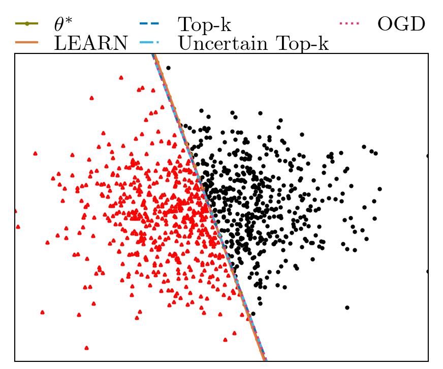
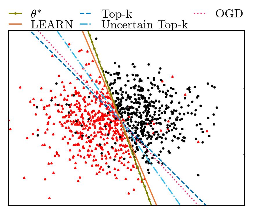
Visualizing the Decision Boundary
Refer to caption
(a) $k=0$
Refer to caption
(b) $k=\sqrt{T}$
Refer to caption
(c) $k=T^{\frac{2}{3}}$
Refer to caption
(d) $k=\frac{T}{4}$
Figure 5: Visualization of Decision Boundary in Presence of Varying Number of Outliers ($k$).

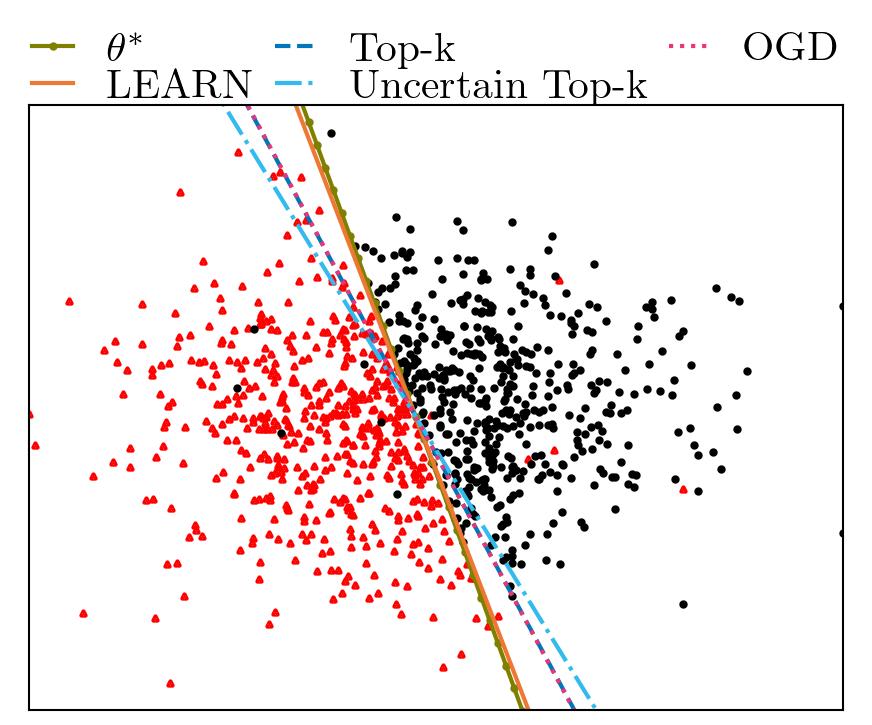
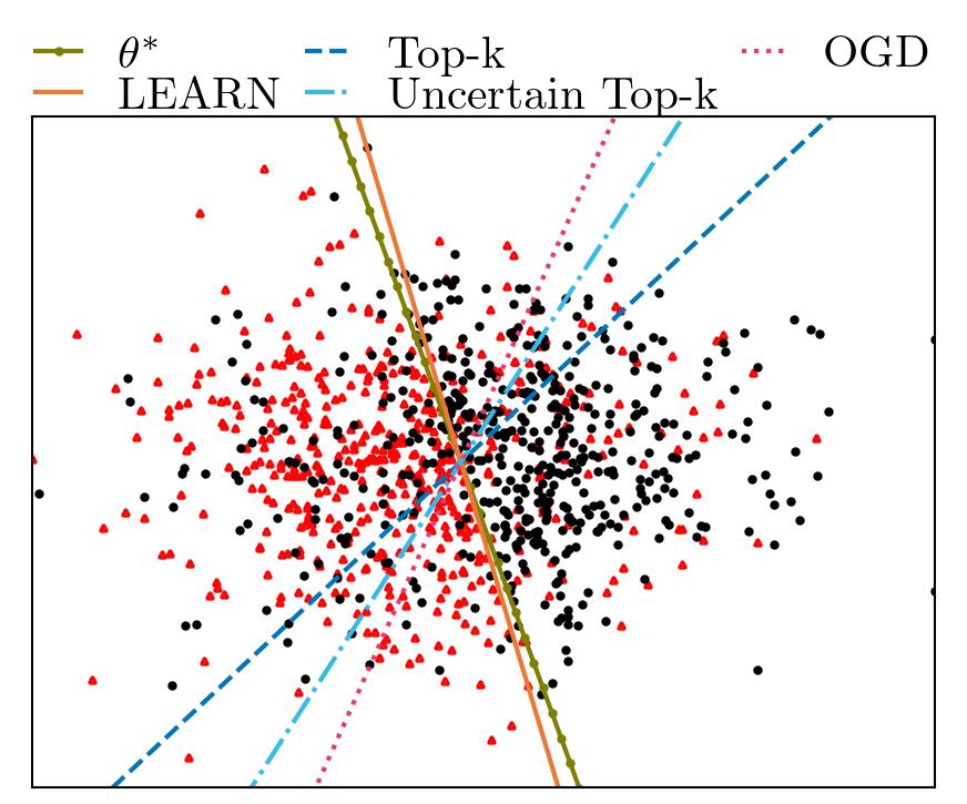
As the data (side information) adheres to a noiseless generative model, the online SVM problem can be thought of as a learning task where the objective is to learn the classification parameter $\theta^{*}$. The decision boundaries learned by different methods with varying numbers of outliers are illustrated in Figure 5 for a single run. The decision boundary for $\theta^{*}$ (plotted as $\langle\theta^{*}\,,x\rangle=0$) is also depicted. To enhance clarity, only $500$ rounds out of the total $T=10^{4}$ rounds are randomly selected for plotting.

In scenarios with uncorrupted data, all methods accurately learn $\theta^{*}$. However, as the number of corrupted rounds increases, the decision boundaries for other baselines gradually deviate from the optimal boundary. In contrast, Learn exhibits robustness against outliers, maintaining a decision boundary close to the optimal configuration even in the presence of corrupted data.

I.3 Online Linear Regression

Refer to caption
(a) $k=0$
Refer to caption
(b) $k=\sqrt{T}$
Refer to caption
(c) $k=T^{\frac{2}{3}}$
Refer to caption
(d) $k=\frac{T}{4}$
Figure 6: Clean Dynamic Regret for Online Linear Regression in Presence of Varying Number of Outliers ($k$).

In our subsequent experimental setup, we undertook a comparative analysis, juxtaposing the performance of Learn against other baseline methods for a regression problem. Specifically, we explored the online ridge regression setting. The details of this experimental configuration are elaborated below:

Uncorrupted Data Generation

The data for uncorrupted rounds ($t\in\mathcal{S}$) adhered to a specific data generation process:

$\displaystyle y_{t}=\langle\theta^{*}\,,x_{t}\rangle+e_{t}$ (151)

In this context, the entries of $\theta^{*}\in^{100}$ were uniformly drawn at random from the interval $[-1,1]$, followed by normalization to a unit norm. Note that st=(xt,yt)subscript๐‘ ๐‘กsubscript๐‘ฅ๐‘กsubscript๐‘ฆ๐‘กs_{t}=(x_{t},y_{t}) is again the side information. The entries of $x_{t}$ for uncorrupted rounds were independently drawn from a normal distribution $\mathcal{N}(0,1)$. Additionally, a small additive noise $e_{t}$ was independently chosen from $\mathcal{N}(0,10^{-6})$.

Corrupted Data Generation

We conducted a total of $10^{5}$ rounds, providing the adversary with the flexibility to corrupt any $k$ out of the $T$ rounds, with the choice made uniformly at random. The experiments covered scenarios where $k$ assumed values from the set $\Big{\{}0,\sqrt{T},T^{\frac{2}{3}},\frac{T}{4}\Big{\}}$. In the context of corrupted rounds, $y_{t}$ was chosen uniformly at random from the interval $[0,1]$.

Strongly Convex Loss Function

We employed the following fixed loss function $f_{t}$ for each round:

$\displaystyle f_{t}\big{(}(x_{t},y_{t}),\theta\big{)}=\frac{\lambda}{2}\|\theta\|^{2}+(y_{t}-\langle x_{t}\,,\theta\rangle)^{2}~{}.$ (152)

The parameter $\lambda$ was set to $10^{-4}$. To enforce an unbounded domain for $\theta$, we considered it to be an element of 100. In each round, the comparator $\theta_{t}^{*}$ was selected by minimizing the function $f_{t}((x_{t},y_{t}),\theta)$ as defined in Equation (152). Although it may not precisely match the ground truth $\theta^{*}$ due to the low influence of additive noise, our experimental results indicate its proximity to $\theta^{*}$.

Choice of Parameters

In the context of Learn, the parameter $a$ was set to $10$, and $b$ was held at $10$. Once again, this choice resulted from a grid search across a limited range of values, with no dedicated tuning efforts for optimality. Consistently, across all methods, including both baselines and Learn, a uniform step size of $\alpha=\frac{1}{\sqrt{T}}$ was utilized.

Results

The experiments were executed across 30 independent runs, and the outcomes are presented in Figureย 6. The results show the similar behavior as in the case of online SVM. We recall them here in the context of ridge regression:

  • โ€ข

    Similar to Sectionย I.2, Learn again employs a cautious update strategy, evident in the gap in clean regret in Figure 6(a). Unlike other baselines, Learn accumulates initial regret due to its cautious update mechanism designed for anticipating corrupted rounds, leading to slow flattening of the regret curve.

  • โ€ข

    In the presence of outliers (until Figureย 6(d)), Learn remains robust, maintaining a maximum regret around $1000$, while other baselines experience a sharp surge in regret.

  • โ€ข

    In our experiments, due to low noise levels, Learn captures the underlying ground truth, sustaining a flat region in Figuresย 6(a) to 6(c) even with outliers. This contrasts with other methods struggling to achieve sustained flatness. OGD, in particular, proves susceptible to outlier influence.

  • โ€ข

    A constant proportion of outliers adversely affects all methods, as expected from Theoremย 3.5. Learn starts accumulating increasing regret when $k=\frac{T}{4}$, depicted in Figureย 6(d), with all baseline methods exhibiting poor performance in this regime.

Discussion on the choice of the step size for baselines

To clarify our choice of step size in the experiments: while it is theoretically possible to set $\alpha_{t}=\frac{1}{mt}$ given that the losses are $m$-strongly convex, we encountered a situation where the value of $m$ was extremely small ($m=\lambda=10^{-4}$). This led to an excessively large step size, causing the anticipated regret bound of $\mathcal{O}(\frac{\log T}{m})$ to become quite substantial. Upon numerical evaluation, we found that using $\alpha=\frac{1}{\sqrt{T}}$ produced a significantly smaller regret for the baselines. As a result, we adopted this more favorable step size in our experimental framework.