On the Peril of Inferring Phytoplankton Properties from Remote-Sensing Observations
Abstract
Remote-sensing satellites are the only means to observe the entire ocean at high temporal cadence. Since 1978, sensors have provided multi-band images at optical wavelengths to assess ocean color. In parallel, sophisticated radiative transfer models have been developed to account for attenuation and emission by the Earth’s atmosphere and ocean, thereby estimating the water-leaving radiance or and remote-sensing reflectance . From these measurements, estimates of the absorption and scattering by seawater are inferred. We emphasize an inherent, physical degeneracy in the radiative transfer equation that relates to the absorption and backscattering coefficients and , known as inherent optical properties (IOPs). This degeneracy arises because depends on the ratio of to , meaning one cannot retrieve independent functions for the non-water IOPs, and , without a priori knowledge. Moreover, water generally dominates scattering at blue wavelengths and absorption at red wavelengths, further limiting the potential to retrieve IOPs in the presence of noise. We demonstrate that all previous and current multi-spectral ocean color satellite observations lack the statistical power to measure more than three parameters total to describe and . Due to the ubiquitous exponential-like absorption by color dissolved organic matter (CDOM), detritus, and non-pigmented biomass at short wavelengths ( nm), multi-spectral do not permit the detection of phytoplankton absorption without very strict priors. Furthermore, such priors lead to biased and uncertain retrievals of . Hyperspectral observations may recover a fourth and possibly fifth parameter describing only one or two aspects of the complexity of . These results cast doubt on decades of literature on IOP retrievals, including estimates of phytoplankton growth and biomass. We further conclude that PACE will greatly enhance our ability to measure the phytoplankton biomass of Earth, including its geographic and temporal variations, but challenges remain in resolving the IOPs.
Nature Communications
Affiliate of the Ocean Sciences Department, University of California, Santa Cruz Department of Astronomy & Astrophysics, University of California, Santa Cruz Kavli IPMU Scripps Institution of Oceanography, University of California, San Diego
J. Xavier Prochaskajxp@ucsc.edu
1 Introduction
Phytoplankton play essential roles within our ecosystem, serving as the base of the ocean food web and performing of all photosynthesis on Earth. Therefore, assessing phytoplankton growth and death – especially in a changing climate (Behrenfeld \BOthers., \APACyear2016; Flombaum \BOthers., \APACyear2020) – is critical to any effort to track and predict the health of our planet. Decades of phytoplankton research have revealed significant regional variations in these process and demonstrated that phytoplankton are highly dynamic on relatively short time scales (hours to weeks, especially in coastal areas, due to tides, upwelling, pulses of freshwater inflow, and other episodic events (e.g. Cloern \BBA Jassby, \APACyear2010). To identify any long-term trend, therefore, one must first develop a detailed picture of the variations on seasonal and shorter timescales.
Unfortunately, our ability to measure phytoplankton in-situ is greatly hampered by the vast expanse of the ocean. Measurements with high temporal frequency can only be acquired at select, fixed stations such as OceanSITES (Boss \BOthers., \APACyear2022). Therefore, oceanographers have turned to remote-sensing satellite observations to perform high-cadence, global analyses of the ocean surface. Beginning with the Coastal Zone Color Scanner experiment (Hovis \BOthers., \APACyear1980), multi-band observations in optical channels have enabled the inference of the concentration of phytoplankton and other seawater constituents, e.g. colored dissolved organic matter (CDOM) and detritus. These inferences are retieved from satellite-derived remote sensing reflectance , which represents the water-leaving radiance normalized by incident solar irradiance. These are defined and recovered by their absorption and backscattering coefficients , , so-called inherent optical properties (IOPs).
The underlying physics for IOP retrievals is radiative transfer: the absorption and scattering of sunlight by seawater modulates and directs incident sunlight back to the satellite. While the radiative transfer physics is straightforward (but not simple; C\BPBID\BPBIe. Mobley, \APACyear2022), there are many factors that complicate the calculations. These include but are not limited to: the concentration of the constituents (typically the desired unknown), their variation with depth, the precise wavelength dependence of the absorption and scattering coefficients of each constituent, geometric factors associated with the Sun’s location relative to the satellite. In addition, Earth’s atmosphere attenuates the signal and introduces a dominant background radiation field which must first be estimated and subtracted (“corrected”) which fundamentally limits the precision of any space-based estimation.
For decades, researchers have attacked this radiative transfer problem to attempt retrievals of scientifically valuable quantities including an estimate of the phytoplankton biomass. There is a robust and well-founded literature describing (and performing) the translation of so-called apparent optical properties (AOPs, e.g. ) to inherent optical properties (IOPs; , ) that depend solely on the water constituents and the water itself. Ideally, one first parameterizes and then estimates (“retrieves”) the absorption and backscattering spectra of the non-water component , and then infers concentrations of phytoplankton, CDOM, detritus, etc. From these, one may examine the geographic distribution and temporal evolution of fundamental biological processes across the global ocean (Fox \BOthers., \APACyear2022).
During the development of a diverse set of IOP retrieval algorithms for this purpose (see Werdell \BOthers., \APACyear2018, for a review), the ocean optics community has acknowledged key challenges to the problem largely independent of those associated with radiative transfer. These include uncertainties related to the atmospheric corrections, non-uniqueness between common constituents (e.g. CDOM and detritus), and retrieving multiple unknowns from limited datasets (e.g. multi-spectral observations). A few, sparsely-cited works have also highlighted a far more fundamental obstacle to the process: a physical “ambiguity” in the inversion of the radiative transfer equation (Sydor \BOthers., \APACyear2004; Defoin-Platel \BBA Chami, \APACyear2007). Unfortunately, this problem has often been confused or conflated with the statistical limitations of an insufficient number of bands measuring (Werdell \BOthers., \APACyear2018; Cetinić \BOthers., \APACyear2024). As such, while the community has acknowledged challenges to IOP retrievals from remote-sensing observations, rigorous assessment of the algorithms themselves has been limited and usually only performed in the context of comparisons to sparse, in-situ observations (e.g. Lee, \APACyear2006; Seegers \BOthers., \APACyear2018).
Another fundamental aspect of the problem is that we do not know the optimal basis functions that describe and nor even the complete set (Garver \BOthers., \APACyear1994). Indeed, it is an aspiration within the ocean color field to recover (or even discover) the composition of phytoplankton (e.g. Mouw \BOthers., \APACyear2017). The ocean color research community has hoped that the main limitation is the sparsity of existing multi-spectral bands provided by current satellites and that hyperspectral observations will lead to a major breakthrough. Indeed, Cael \BOthers. (\APACyear2023) has demonstrated from a data-driven analysis of data its limited information content, i.e. only degrees-of-freedom in multi-spectral, satellite observations. But they also concluded that in-situ hyperspectral datasets offer only one or two addition degrees of freedom. In this manuscript, we examine this question from a new angle – with the standard approach of IOP retrievals – and reach similar conclusions.
Here, we introduce the Bayesian INferences with Gordon coefficients (BING) package for ocean retrievals in a Bayesian context. Our approach follows many of the standard assumptions of widely adopted algorithms in the literature, e.g. the generalized IOP (GIOP) model (Werdell \BOthers., \APACyear2013), the Garver-Siegel-Maritorena (GSM) algorithm (Maritorena \BOthers., \APACyear2002). In addition, we emphasize and expand upon the “ambiguity” problem – a physical degeneracy in the radiative transfer equation that couples reflectances to IOPs – which fundamentally limits IOP retrievals. In turn, we demonstrate that IOP retrievals from multi-spectral datasets constrain at most three parameters describing and . Therefore, if one allows for the fact that the spectral shape of CDOM absorption varies and is unknown, then we show one cannot retrieve a measurement of phytoplankton absorption. This includes all previous missions with satellites carrying multi-bands sensors. We then examine the prospects for IOP retrievals with hyperspectral observations and discuss additional opportunities to address the deep degeneracies that lurk within.
2 The Bad: A physical degeneracy in the radiative transfer
At the heart of our analysis is a new Bayesian inference algorithm for the retrieval of IOPs from remote sensing reflectances, the BING package. The primary motivations for introducing a Bayesian framework are twofold: (i) it forces one to explicitly describe all of the priors that influence the result; and (ii) it permits well-established approaches for performing model selection, i.e., estimating the maximum number of free parameters one can use to describe the data.
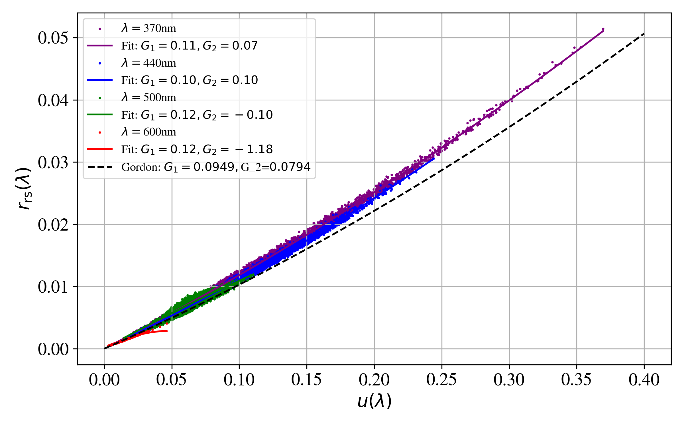
To construct any such algorithm, one must have a well-defined forward model to predict the observables, here remote-sensing reflectances . For IOP inversion, this means a radiative transfer model – or its approximation – which estimates from and the backscattering coefficients . The majority of IOP retrieval algorithms developed by the community have used the quasi single-scattering approximation (QSSA) originally introduced by Hansen (\APACyear1971) and translated to ocean color by Gordon (\APACyear1973) (see also Zege \BOthers., \APACyear1991). This approach was refined further by Gordon (\APACyear1986) who approximated the sub-surface remote reflectances with a Taylor series expansion:
| (1) |
with
| (2) |
Most IOP retrieval algorithms have taken and set the coefficients as constants and , i.e. values independent of wavelength. In this manuscript and for the default mode of BING, we adopt the same prescription and coefficients, but scrutinize the accuracy of this assumption in Supp 6.2. For the results in the main text, we assume a perfect forward model, i.e. we use Equation 1 to generate the target and perform the fits on these values. In practice, we work with remote-sensing reflectances following a standard conversion from (Lee \BOthers., \APACyear2002):
| (3) |
For the development and testing of BING, we have leveraged a large set of , spectra made public by Loisel \BOthers. (\APACyear2023) (hereafter L23). We use their model which includes inelastic scattering (not relevant here) and the Sun at the zenith. The IOP spectra were generated from their database of in-situ measurements of phytoplankton and models of several additional constituents: CDOM , pure seawater , and detritus . L23 then generated estimates of the backscattering coefficients following standard assumptions based on in-situ and laboratory work (see Loisel \BOthers., \APACyear2023, for additional details). These 3,320 and spectra define our dataset and range from 350-750 nm at nm sampling.
Despite the approximation of Equation 1, it does capture a salient aspect of the physics: the functional dependence of on and thereby the IOPs and . However, this dependence is the “bad” aspect of IOP retrievals: because is a function of the ratio of /:
| (4) |
the radiative transfer solutions are physically degenerate in /. Put succinctly, any IOP solution that recovers a set of observations can be replaced by an infinite set that preserves the / ratio. Therefore, the retrieval is only tractable if one implements strong constraints (known as priors in Bayesian analysis) on the functional forms of and .
In the following section, we examine the consequences of this physical degeneracy on IOP retrievals. We describe several standard priors from previous work and describe their impacts on IOP retrieval. Section 6.3 of the Supplement provides full details on BING and our specific approach to perform the Bayesian inference. We have also implemented standard minimization (Levenberg-Marquardt) as a fitting option to speed-up model development and portions of the analysis. For results in the main text, we assume constant signal-to-noise () for the measurements unless otherwise specified.
Note that the Bayesian approach in BING involves using Bayes’ theorem to update the probability of a hypothesis based on prior knowledge and new data. When retrieving IOPs from , this approach explicitly incorporates all available prior information about the IOPs and their uncertainties into the model. By doing so, it allows for a more transparent and rigorous estimation process. The Bayesian framework considers the likelihood of the observed given the IOPs and combines it with the prior probability distributions of the IOPs to obtain a posterior distribution. This posterior distribution provides a probabilistic solution to the inverse problem, highlighting the most likely values of the IOPs while quantifying the uncertainties, leading to more reliable and informed retrievals.
3 The Good: Water as a prior
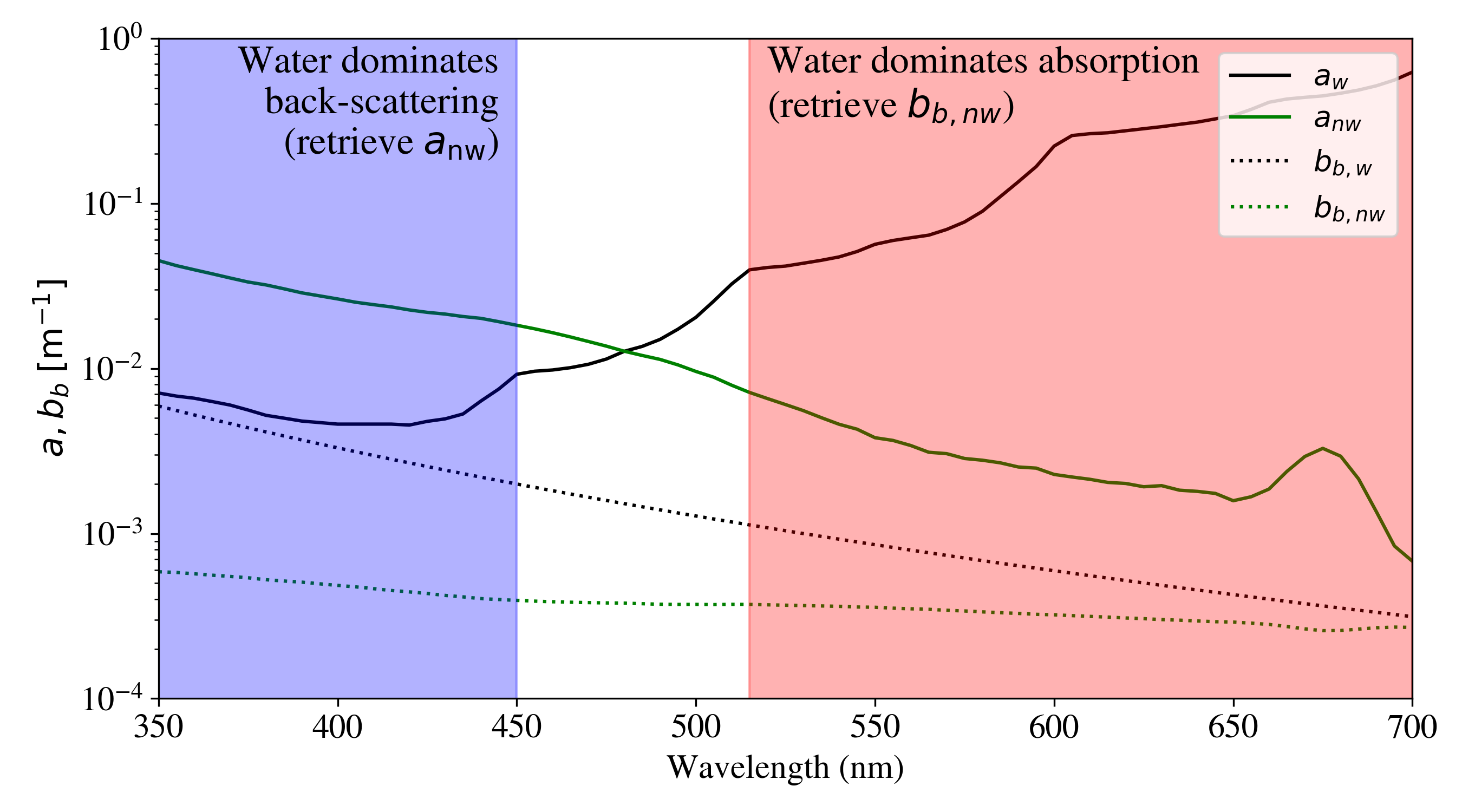
The “good” aspect of IOP retrievals is the presence of water which introduces an ever-present and precisely known111Except in the ultraviolet, nm, which is intentionally ignored in this manuscript; Mason \BOthers. (\APACyear2016). constraint on the problem. The absorption and backscattering spectra of pure seawater impose priors on the model that serve to partially alleviate the physical degeneracy described in the previous section. First, and span the entire spectrum and therefore couple the otherwise independent values. Second, to the extent that the shapes of and are unique relative to other constituents this helps one avoid the / degeneracy. Third, the strong absorption of water at nm and the relatively high magnitude of at nm define regions where one may retrieve information on the non-water components.
On the last point, Figure 1 compares the absorption and backscattering coefficients of water against one example of non-water spectra , from the L23 dataset. As emphasized in the Figure, at red wavelengths and such that the observations may constrain . Similarly at nm, and such that the observations constrain . These inferences from Figure 1, however, rely on the strong (but frequently satisfied) prior that at nm and at nm. If this is relaxed, e.g. if and may take on any values then the / degeneracy forces an infinite set of solutions (i.e. no unique retrieval is possible; see Supp 6.4).
Stated another way, the greater the freedom that one allows for or , the more degenerate the solutions. This fundamentally limits our ability to retrieve arbitrary or even in the presence of perfect data (infinite number of channels and no uncertainty). Therefore, no algorithm222Including our own initial efforts with a more sophisticated algorithm than BING. can aim to retrieve arbitrary (Loisel \BBA Stramski, \APACyear2000; Loisel \BOthers., \APACyear2018) or even highly complex and (e.g. Chase \BOthers., \APACyear2017). To make progress, one most also impose strong constraints on and to recover unique or most probable solutions. These priors, however, must insure that the values of and cannot vary at any individual wavelength where one seeks a retrieval in a way which holds their ratio constant.
4 The Ugly: Actual IOP retrievals
Let us now perform the “ugly”: attempted retrievals of and using assumed spectral shapes (priors) with a set of increasingly complex prescriptions. We follow common practice for models of and which have been informed by in-situ and laboratory measurements of ocean constituents. In turn, we will examine the maximum complexity that can be statistically constrained by observations designed to mimic satellite retrievals, e.g. data from multi-band and hyperspectral observations.
Consider first the simplest scenario we may conceive: a two-parameter model with both and taken as constant at all wavelengths:
| (5) | |||||
| (6) |
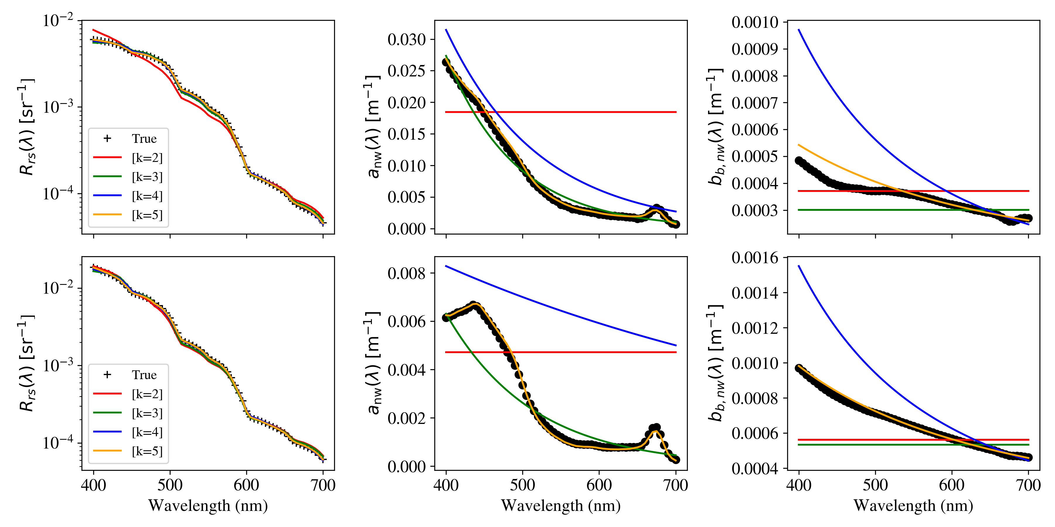
We have fitted this model – including seawater absorption and backscattering – to two examples from the L23 dataset (Figure 2): one chosen to be representative of their full sample and the other chosen to have a higher than typical phytoplankton absorption relative to the combined CDOM and detritus components (i.e. ). For these, we fit to values calculated directly from Equation 1 and assume a constant for the values for the likelihood calculation333The best fits are identical for any constant .. Despite the extreme simplicity of this model, the fits are not too dissimilar from the true values, especially for the high example444This -dominated spectrum has a low total non-water absorption, i.e. weak absorption.. This follows from our discussion of Figure 1: water backscattering and absorption dominates the solution at short and long wavelengths respectively and the non-water components have limited impact on the , i.e. we primarily measure seawater from IOP retrievals especially for ocean waters with low chlorophyll concentrations.
We consider three additional models of increasing complexity: the model,
| (7) | |||||
| (8) |
the model,
| (9) | |||||
| (10) |
and the model,
| (11) | |||||
| (12) |
where is expressed in nm. A power-law is frequently adopted to describe , especially that related to particulate matter (Gordon \BBA Morel, \APACyear1983). Here we allow to vary but consider fixed exponents in several models discussed in the Supplements. An exponential function, meanwhile, is commonly used to describe absorption by CDOM and/or detritus (Stramski \BOthers., \APACyear2001). In-situ absorption measurements show typical values of for CDOM (Roesler \BOthers., \APACyear1989) and for detritus (Stramski \BOthers., \APACyear2001). Our fiducial models only require and we discuss stricter priors on that parameter below (and in Supp 6.6).
The component in Equation 11 is introduced to capture “typical” absorption by phytoplankton. It is expected and observed that this component may exhibit the greatest complexity. Indeed, scientifically the community aims to distinguish the potentially large variations in phytoplankton families throughout the ocean and inland waters. Here, we adopt the parameterization of Bricaud \BOthers. (\APACyear1995):
| (13) |
with the Chlorophyll-a concentration in mg/m3 and the tabulation of and are provided by Bricaud \BOthers. (\APACyear1998). We further set to the value used by L23,
| (14) |
This last step is effectively another prior, but we will not penalize this model for the additional information in the analysis that follows.
Figure 2 shows the best solutions derived with BING for the models. While the log-scaling of the panels hides differences at the few percent level, it emphasizes that one requires nearly perfect observations to distinguish between the various models. The model matches the data to within 10% at all wavelengths and the and models achieve several percent or less. As a result, the model yields a reduced chi-squared if we assume errors (=20) in the values. Visually, at least, Figure 2 emphasizes the (ugly) challenge of performing IOP retrievals: one is severely limited in the degree of unique information that can be derived.
We examine these points further in the Bayesian context by applying standard approaches for model selection, i.e., assessing the balance between model fit and complexity. Specifically, we have evaluated the Aikake and Bayesian information criteria (AIC,BIC) which are akin to -difference tests (Bentler \BBA Bonett, \APACyear1980):
| (15) |
and
| (16) |
with the number of measurements and the likelihood function calculated assuming Gaussian statistics for uncertainties . The likelihood function quantifies the probability of observing the data given the specific forward model and its parameters. Since it is calculated under the assumption of Gaussian (normal) statistics for the uncertainties, this means that the observed data, i.e., the measurements, are assumed to be normally distributed around the model predictions with the standard deviation. For our hyperspectral analysis where , the BIC offers a more stringent constraint but the results with AIC are qualitatively similar. A high AIC or BIC value implies that the model is less likely to be the best model given the data, considering both the fit and complexity. In the main text, we assess model selection by evaluating the difference in BIC for any two models where indicates that model is preferred and vice versa.
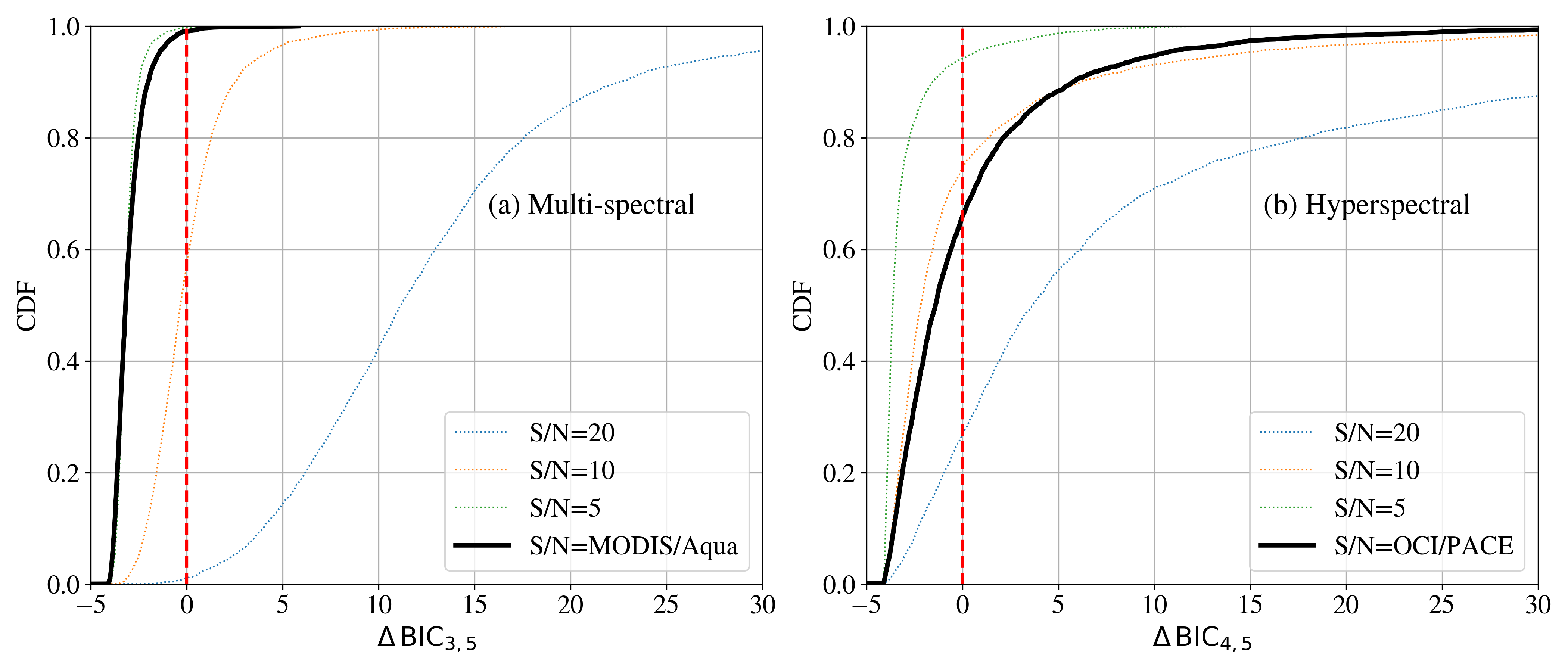
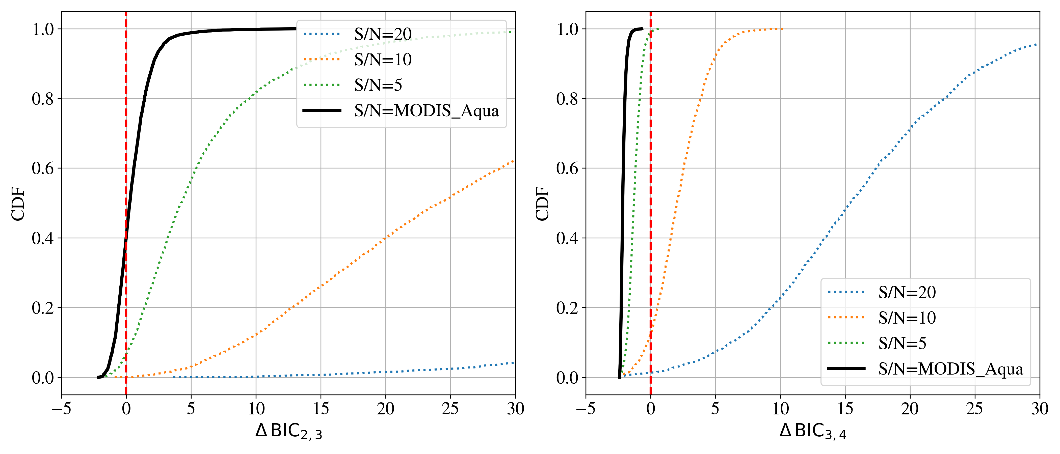
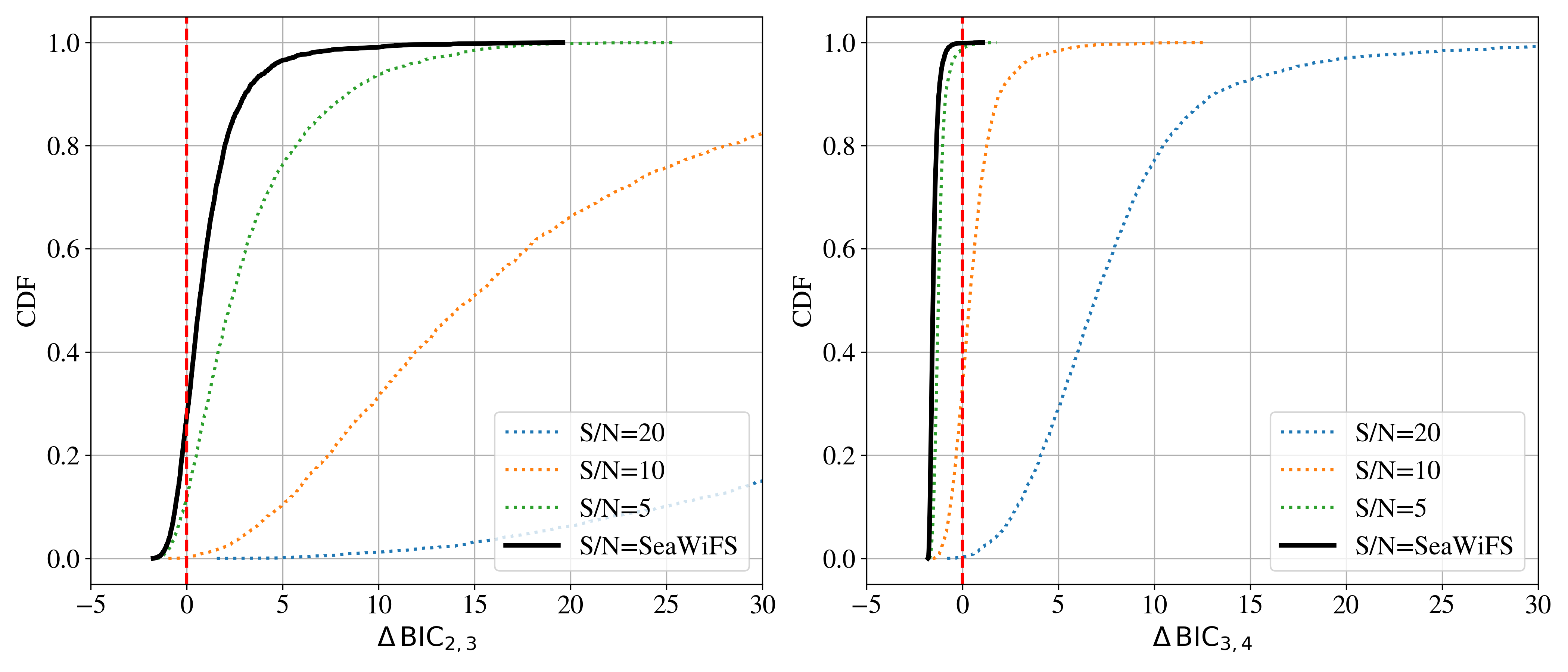
Figure 3 shows the values for simulated Moderate Resolution Imaging Spectroradiometer (MODIS) observations of the L23 spectra (see Supp 6.1 for details). The cumulative distribution function (CDF) on the y-axis represents the cumulative probability that the values for the 3,320 fits to the L23 data are less than or equal to a specific value. Each value corresponds to a comparison between two models, specifically the BIC values for a model with and without phytoplankton parameters ( and in the multi-spectral case, Figure 3a, and and in the hyper-spectral case, Figure 3b). If the CDF value is at a specific value, it means that the of the values in the dataset are less than or equal to that specific value. Thus, the CDF curve shows the proportion of the dataset for which the simpler model is preferred as a function of the value. The higher the CDF value at , the higher fraction of the dataset which favors the simpler model over the more complex one.
For the analysis with a realistic MODIS noise model, fewer than 1% of the spectra prefer the model with phytoplankton. This holds true even though our analysis assumed a perfect forward model and perfect knowledge of the measurement uncertainties, without correlated errors. Allowing for these uncertainties would result in zero cases with . In fact, we find (Supp. Figure 9) that one cannot retrieve more than 3 parameters from MODIS observations and that even the model is largely satisfactory. Without perfect knowledge of the absorption by CDOM one cannot retrieve phytoplankton from MODIS observations alone.
The curve corresponding to in Figure 3a shows that while there is some support for the simpler model, indicated by the CDF values for positive , the more complex model, which includes additional parameters for phytoplankton, is generally preferred. This is because the CDF for negative values is low, indicating that the simpler model is not favored in most of the dataset. In other words, although the simpler model is supported in some cases, the overall trend indicates that the more complex model is usually favored for . Thus, reducing noise in the data is essential when increasing model complexity. However, achieving is challenging, even at blue wavelengths in open ocean Case 1 waters, as demonstrated in numerous validation studies (6.1). And, achieving at nm where absorption by seawater alone is very high may be impossible (Zhang \BOthers., \APACyear2022).
We reach even stronger conclusions for simulated SeaWiFS observations (Supp 6.1) which have fewer bands. Unless one identifies an approach to regularly achieve measurements in the presence of all error terms (e.g. atmospheric corrections), phytoplankton cannot be retrieved from multi-spectral observations without strong, additional priors. In Supp 6.7, we examine the GIOP and GSM models which assume a fixed and steep shape parameter and the negative outcomes of this assumption.
Now consider an assessment using L23 spectra with simulated Ocean Color Instrument (OCI) hyperspectral observations on the Plankton, Aerosol, Cloud, ocean Ecosystem (PACE) sattelite (see Supp 6.1 for details). Our fiducial case uses the L23 spectral sampling and we limit the observations to nm, outside of which systematics of the L23 dataset and instrumentation dominate the uncertainties in , and poor knowledge of the wavelength dependence of the ocean’s constituents preclude confident analysis. Figure 3 shows the distribution in the difference in BIC values, , between the models assuming several choices for the and our estimate for the OCI/PACE noise from v1.0, Level 2 products (Supp 6.1). We find that OCI/PACE may not recover an assemblage signature of phytoplankton from water with properties similar to those represented by the L23 dataset. We are led to conclude that one can may retrieve four parameters for IOPs from a OCI-like observation and possibly a fifth. Two of these numbers describe the amplitude and shape of parameterized as an exponential and two numbers describe modeled as a power-law. Absent strong priors that account for one of these four, extracting even one number describing (at all wavelengths) will be challenging.
5 Conclusions and Future Prospects
In this manuscript, we have introduced BING, a Bayesian inference algorithm for IOP retrievals utilizing the Gordon coefficients for radiative transfer. We have reemphasized a known but under-appreciated physical degeneracy in the radiative transfer – is a function of / which strictly limits one ability to retrieve and without strong priors. Two of the priors are natural: water both absorbs and scatters light with precisely known coefficients, at least for wavelengths nm. We demonstrated, however, that even these constraints are insufficient; indeed, water frequently dominates the model limiting the extraction of additional information. Consequently, we found that multi-spectral observations with published uncertainties Zhang \BOthers. (\APACyear2022) cannot reliably retrieve phytoplankton, and that even hyperspectral observations (e.g. OCI/PACE) will be challenged (Figure 3).
While the ill-posed nature of the inversion problem to retrieve IOPs from is a known issue, this study offers significant value by providing a comprehensive analysis and quantification of this degeneracy. The methodology rigorously examines the implications of spectral ambiguities on satellite-derived IOP products, highlighting the specific conditions and parameters where these ambiguities are most pronounced. This detailed investigation not only reinforces the necessity for caution in interpreting satellite products, but also advances the understanding of the limitations and potential improvements in current algorithms. By revealing the extent and impact of these ambiguities, the study contributes insights for the refinement of remote sensing techniques and the development of more accurate ocean color models. Consequently, this work is a crucial step forward in enhancing the precision and reliability of ocean color remote sensing.
Previously, Cael \BOthers. (\APACyear2023) reached a similar inference as one of our primary conclusions – the limited information content of remote-sensing observations. Specifically, they analyzed the degrees of freedom (DoF) of data through a standard principal component analysis finding that in-situ data with MODIS sampling has only 3 DoF and inferred only DoF=2 for remotely sensed . Our analysis, which includes several constraints, such as water absorption and scattering, yields at least one additional parameter but the overarching implication is similar: retrievals from observations have limited information content.
On statistical grounds the community could not and cannot retrieve from provided one allows for exponential absorption by CDOM and/or detritus which are always present. In fact, this component () tends to exceed , even in the open ocean (Siegel \BOthers., \APACyear2013; Hooker \BOthers., \APACyear2020). Previous work that published estimates of required very strict priors on the shape of (Supp 6.6), leading to significant bias in estimates of . In the cases where was allowed to vary (Boss & Roesler, Chapter 5 Lee, \APACyear2006), the errors on were severe and limited retrievals only to upper limits on , consistent with this work.
Do our results therefore invalidate the past several decades of research and data products using satellite-based ocean color observations? At the least, all previous retrievals from must be further scrutinized. We assert uncertainties and biases were frequently (possibly always) underestimated, and substantial correlations between retrieved parameters will be present. Unfortunately even relative analyses of may be subject to large error. There are, however, key products that are primarily (and very nearly exclusively) empirical, i.e. generated without any radiative transfer model (Stramski \BOthers., \APACyear2022). These empirically-based algorithms may circumvent the radiative transfer issues raised here, but as emphasized by Cael \BOthers. (\APACyear2023), one cannot retrieve an arbitrary number of such quantities from visible domain observations. Therefore, the suite of products generated by the community to date are highly coupled and correlated. The limited information content of measurements subject to realistic uncertainties is inherent to the problem.
While the results from Figure 3b indicate that hyperspectral observations offer a substantial improvement over multi-spectra data, even detecting phytoplankton remains challenging. We reemphasize that the results presented here have assumed a perfect forward model (i.e. no error in the radiative transfer calculation), uncorrelated uncertainties, a perfect model for water absorption and backscattering, and homogeneous seawater (no vertical or horizontal spatial variations). Furthermore, even if we surmount these issues, we may only be able to extract a single parameter describing phytoplankton, e.g., the amplitude at nm. And, strictly speaking, this may be attributed to any absorption component (not solely ) that does not follow the exponential described by CDOM and detritus.
How might we proceed? It is abundantly clear that we must identify the optimal way to parameterize the problem to make most effective use of the 4 or 5 parameters that describe and . For example, if we know (i.e. fix its value as a prior), we would not “waste” a free-parameter to estimate its value. In short, we must harness our knowledge of the ocean from previous in-situ measurements (or current, if one can afford them) to set priors on the model. These priors should be geographically and temporally variable to reflect different oceanic conditions. Because strict and biased priors have been shown to lead to inaccurate and uncertain retrievals, one must proceed cautiously. Empirically derived priors can help mitigate these issues by providing a more accurate representation of the ocean’s optical properties.
One obvious community-wide effort would be to develop and agree upon strong priors for . This is current practice in many existing algorithms (e.g. GIOP, GSM, which set to a single value), but we describe the negative consequences of this extreme approach in Supp 6.6. Instead, we encourage the community to generate priors as probability distribution functions that vary with geographic location and time and then revisit these in our changing climate. Additionally, we must include more observations, both from space and in-situ. From space, we must leverage the fluorescence signal at nm (Wolanin \BOthers., \APACyear2015) whose production and radiative transfer are distinct from that of IOP retrievals. From the ocean, in-situ observations provide invaluable validation data and may establish priors like those for . Non-visible in-situ optical observations have been shown to improve retrievals of CDOM absorption, and could be retained to better partition signals related to CDOM and phytoplankton biomass. Constraints on , as a function of location and season, and physical priors on the coupling of to for individual components from the physics of absorption and scattering could be impactful.
Developing community-wide Bayesian retrieval algorithms is also recommended. The ocean color remote-sensing community should be encouraged to adopt a Bayesian framework for IOP retrievals such as BING, explicitly including all priors and their uncertainties. A Bayesian approach allows for a more transparent and rigorous incorporation of prior knowledge and uncertainties, leading to more reliable retrievals. Unlike BING, however, Bayesian algorithms must adopt an accurate forward model and its uncertainties, include correlated and systematic error in the observations, and harness new data sources. We have initiated such a project – Intensities to Hydrolight Optical Properties (IHOP) – and encourage community adoption and development. The scientists focused on atmospheric corrections have already embarked on this journey following the original insight of Frouin \BBA Pelletier (\APACyear2015). Ultimately, we should consider merging the two, i.e., generate an end-to-end Bayesian model that fits top-of-atmosphere radiances to retrieve IOPs.
Increasing the spectral resolution of satellite observations can provide more detailed information about the absorption and backscattering properties of phytoplankton, thereby reducing the impact of degeneracies. Thus, the development and deployment of hyperspectral satellites with high spectral resolution across the visible and near-infrared spectrum are recommended. The recently launched PACE satellite will lead the way. Additionally, exploring alternative remote-sensing techniques, such as Lidar and fluorescence-based methods, and incorporating polarization information to complement traditional ocean color observations, should be considered. These advanced techniques may provide independent measurements that help resolve ambiguities and improve the overall accuracy of phytoplankton estimates, although information gained using these new techniques should be clearly demonstrated and defined first in the field.
Addressing the uncertainty in atmospheric corrections is another critical recommendation. Improving atmospheric correction algorithms to reduce the uncertainties they introduce into ocean color retrievals is crucial. Incorporating advanced atmospheric models and ancillary data (e.g., aerosol properties) can enhance correction accuracy. Atmospheric corrections are a significant source of error in remote-sensing reflectance measurements, and reducing these uncertainties is essential for accurate phytoplankton IOP retrievals. Continued implementation of dark-pixel correction schemes, for example, removes non-visible information and is inconsistent with in-situ observations of the aquatic light field.
Promoting interdisciplinary collaboration is also essential. Fostering collaboration between oceanographers, remote-sensing experts, and radiative transfer modelers to address the complex challenges of IOP retrievals can bring together diverse expertise and perspectives, leading to more innovative and effective solutions. These should include individuals with mastery of statistics who can rigorously assess uncertainty and help develop robust and transparent algorithms.
By implementing these recommendations, the remote-sensing community can significantly enhance the accuracy and reliability of phytoplankton IOP retrievals, leading to better-informed biogeochemical models and ecological assessments. This comprehensive approach will help ensure that remote-sensing data accurately reflect the true state of the ocean’s biological and chemical processes, thereby supporting more effective environmental monitoring and management efforts.
6 Supplementary Materials
| Band | |
|---|---|
| (nm) | (sr-1) |
| 412 | 0.0012 |
| 443 | 0.0009 |
| 488 | 0.0008 |
| 531 | 0.0007 |
| 547 | 0.0007 |
| 555 | 0.0007 |
| 667 | 0.0002 |
| 678 | 0.0001 |
Notes: The error has assumed that 1/2 of the variance is due to the in the in-situ measurements.
| Band | |
|---|---|
| (nm) | (sr-1) |
| 412 | 0.0014 |
| 443 | 0.0011 |
| 490 | 0.0009 |
| 510 | 0.0006 |
| 555 | 0.0007 |
| 670 | 0.0003 |
Notes: The error has assumed that 1/2 of the variance is due to the in the in-situ measurements.
6.1 Data and their Uncertainties
As described in the main text, all of the absorption and scattering spectra examined in this manuscript were taken from Loisel \BOthers. (\APACyear2023) (aka, L23). Their dataset includes total absorption and scattering as well as the contributions from individual components (e.g. , , ). The dataset also includes outputs from Hydrolight calculations (C\BPBID. Mobley \BBA Sundman, \APACyear2013) using these spectra as input, e.g. and depth-resolved quantities like the diffuse absorption coefficient . Specifically we use the L23 dataset with inelasctic scattering and at 0 deg. solar and viewing zenith angle.
For many of the analyses presented here, we have independently generated simulated spectra for several multi-spectral and hyperspectral missions. For the fits presented in this manuscript, we ignore the provided by L23 and instead use Equations 1-3 to calculate from and . We then resample these spectra to the bands/channels of several satellite missions:
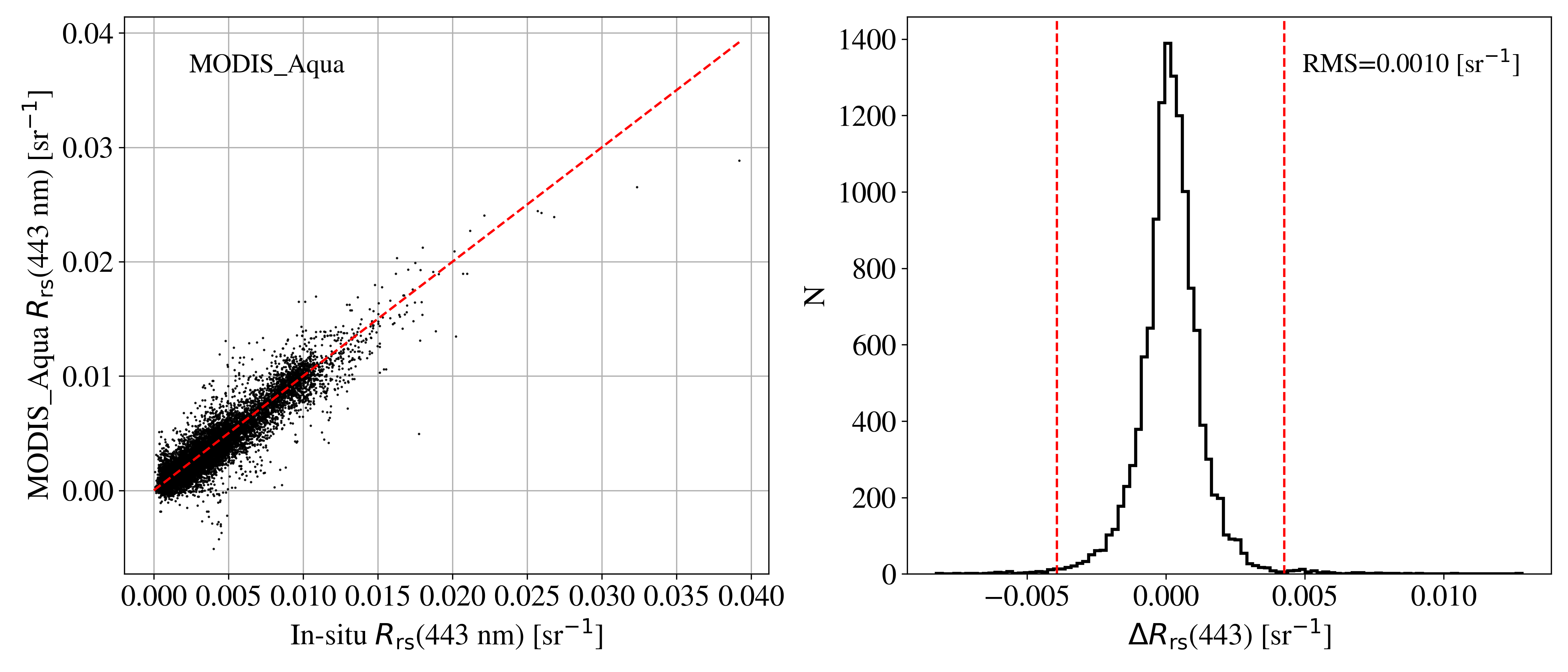
MODIS/Aqua: We adopt 8 multi-spectral bands as listed in Table 1 corresponding to the MODIS Aqua mission and we evaluate at the center of each. For uncertainties, we have estimated the RMS difference between satellite and in-situ “match-up” measurements collated on the SeaBASS database (Werdell \BBA Bailey, \APACyear2002) after iteratively clipping any outliers. Figure 4 shows an example of the data and clipping for one band. We further assumed that one half of the variance is due to the in-situ observations themselves. These RMS values are also provided in Table 1, and we find they are in good agreement with other estimations (Zhang \BOthers., \APACyear2022; Kudela \BOthers., \APACyear2019).
SeaWiFS/SeaStar: We followed a similar procedure for the Sea-viewing Wide Field-of-view Sensor (SeaWiFS) using 6 bands and the uncertainties provided in Table 2.
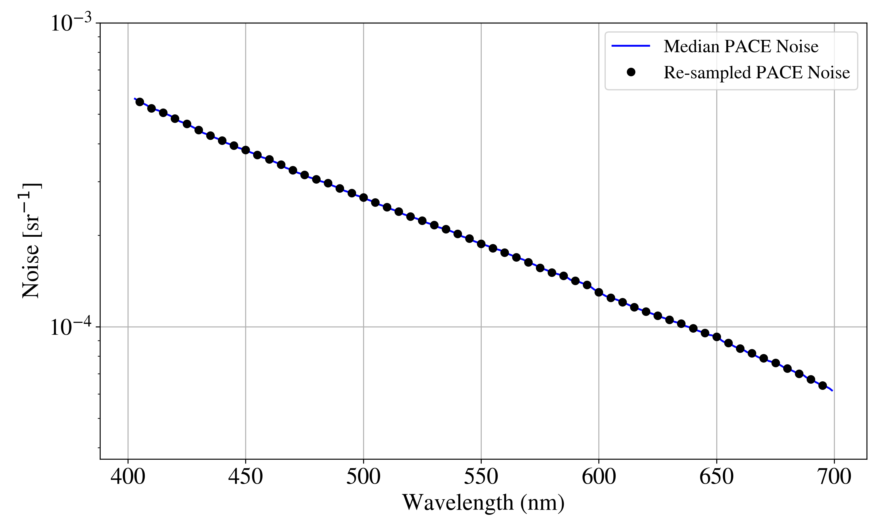
OCI/PACE: For simulated OCI/PACE spectra, we assumed nm sampling and limited the wavelength range from nm. The lower bound is due to (i) greater uncertainties in the atmospheric corrections, (ii) greater uncertainty in water absorption and scattering, (iii) greater uncertainty in how best to parameterize the non-water components in the UV. The upper wavelength bound is to avoid systematics that likely dominate the uncertainty at the lowest signals.
For the PACE noise model, we downloaded a single granule (2,175,120 pixels) of Level 2 data, v1.0: PACE_OCI.20240413T175656.L2.OC_AOP.V1_0_0.NRT.nc. We then took the median uncertainty spectrum (Rrs_unc Zhang \BOthers., \APACyear2022) for all non-flagged data between 33-40N and 73-78W. This median spectrum is plotted in Figure 5 at the Level 2 wavelength sampling ( nm). We also show the values adopted at our nm sampling, and one notes that we did not adjust despite the larger sampling size. This is because OCI is over-sampled at nm, i.e. the data is highly correlated. Further work should assess the degree of this correlation to obtain a better noise estimate. If we were to assume no correlation (i.e. reduce by ), the results in Figure 3b would yield a higher fraction of spectra preferring 5 parameters: instead of of the L23 dataset showing , we find fail the criterion.
6.2 Taylor expansion model re-examined
To examine the use of Equation 1 as an approximation of the radiative transfer, consider Figure 6 which plots the Hydrolight-derived of L23 converted to with Equation 1 against the evaluated values using Equation 2 at 4 distinct wavelengths. These evaluations approximately follow a quadratic with zero y-intercept. Overplotted with a dashed line is the Gordon approximation using the standard coefficients and Equation 1. Qualitatively, the Hydrolight outputs follow the relation yet lie systematically above the curve. At its extreme, the Taylor series approximation is offset by at nm and .
To further illustrate the difference, we have fitted coefficients to the data at select wavelengths and recover similar values but values that vary significantly with wavelength ( at nm, at nm). We also find that there is significant scatter around each of the fits with a relative RMS of at shorter wavelengths and at the reddest wavelengths. We expect this scatter is inherent to Equation 1 and would be unavoidable if one uses this approximation even with wavelength-dependent coefficients. An accurate retrieval algorithm would need to account for these variations or otherwise suffer significant systematic error. This is the focus of a separate algorithm we are developing (IHOP), and we also refer the readers to recent advances in approximations of the radiative transfer equation (Twardowski \BOthers., \APACyear2018).
6.3 Bayesian Inference
Provided the forward model and a parameterization of and , the Bayesian inference is straightforward and a wealth of well-trodden approaches and software packages are available. For BING, we adopt the Monte Carlo Markov Chain (MCMC) formalism which empirically derives the posterior probabilities for the , parameterization including full uncertainties and all of the cross-correlation terms. This requires the definition of a likelihood function , which will have the form:
| (17) |
where represents the measured values, is the full covariance matrix of including correlations, and is the forward model of at the locations of .
It can be shown that an MCMC analysis converges to the exact solution if run for an infinitely long time; in practice, the calculations tend to converge after iterations. For the analysis here, we generally run for 75,000 trials with at least 2 walkers per parameter (and at least 16 walkers) and only analyze the last 7,000 iterations of each. This release of BING uses the EMCEE sampler (Foreman-Mackey \BOthers., \APACyear2013) which was developed for astrophysical applications and has see wide-spread adoption in the field (over 8,000 citations).

6.4 Fits with and/or free to vary
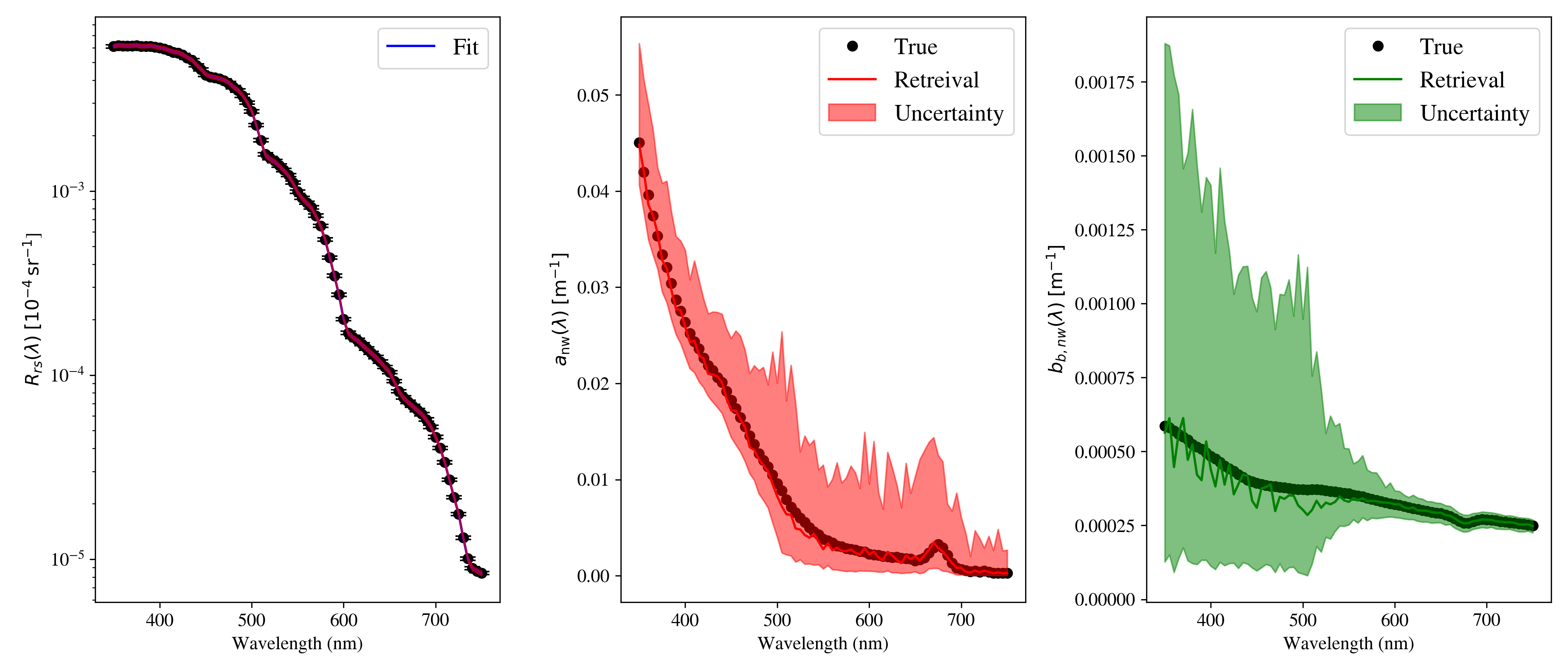
One point emphasized in this manuscript is that one cannot retrieve arbitrary or or even and because of a physical degeneracy in the inversion of the radiative transfer equation (Equation 4). To demonstrate this with two examples, we performed an IOP retrieval of and assuming a perfect forward model (Equation 1), perfect knowledge of the uncertainties, and perfect knowledge of water (, ). In this case, we solve for “arbitrary” and by parameterizing each with 81 free parameters, one per wavelength channel. We show the fits to for the index=170 spectra of L23 in Figure 7 and the retrievals with 95% confidence intervals, finding that our solutions for and start “blowing up” after only 50,000 samples.
To further emphasize the point, we refit the data but constrained to be a power-law with a fixed exponent set at a value that closely corresponds to the known spectrum and only allow the amplitude of to vary in the retrieval. Once again, the solution diverges (Figure 8) although more slowly. If we were to run for infinite samplings, we would recover an infinite uncertainty. With an arbitrary spectrum, we can match any change to the amplitude of and maintain constant . Therefore, even with the strong constraint of water and just a single degree of freedom for , we still cannot retrieve arbitrary . This physical degeneracy limits the information content of retrievals and precludes arbitrary functional forms for and , e.g. models which strive to retrieve arbitrary are ruled out.
6.5 Additional BIC Analysis
We have compared additional pairs of models for the simulated multi-spectral spectra than those in the main text. These additional analyses explore further the conclusion that such datasets are limited to retrieving a total of =3 parameters describing and from multi-spectral, satellite observations.
Figure 9 shows distributions for the vs. model and the vs. model. Remarkably, we find that approximately half of the L23 dataset if optimally described by the constant IOP model. The results in Figure 9 show clearly that the model is disfavored for all of the L23 dataset. This latter result greatly supports the conclusion on multi-spectral data given in the main text. Not surprisingly, the conclusions are even stronger for SeaWiFS spectra (Figure 10).
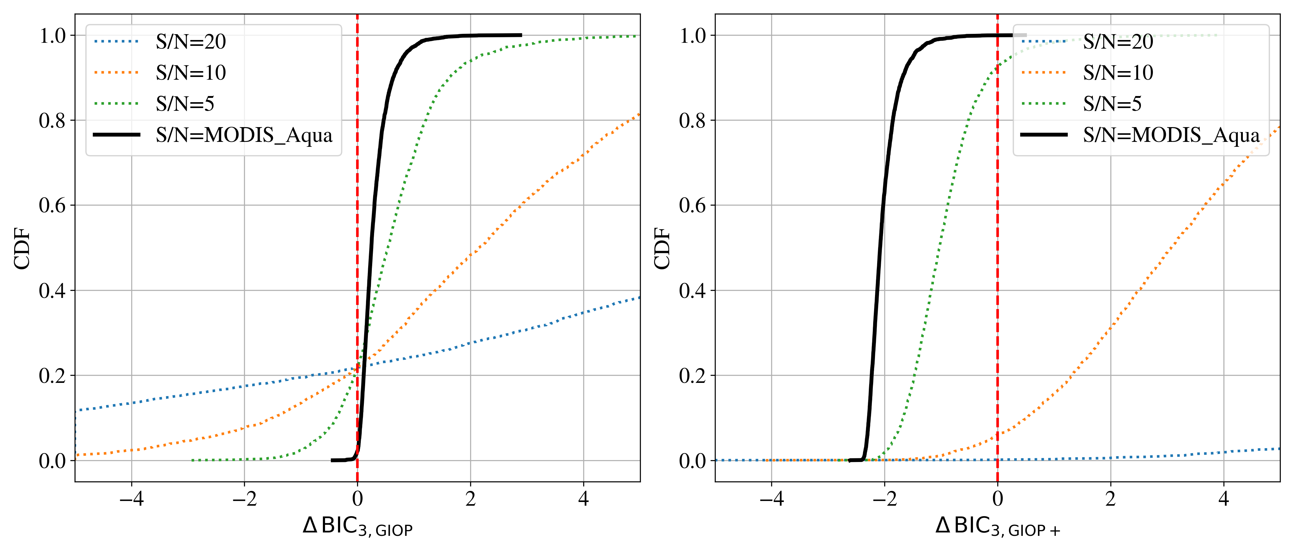
Now consider Figure 11 which presents distributions for two “GIOP” models which assume an exponential component for with fixed shape parameter =0.018, the Bricaud formulation for and either (i) GIOP: the Lee \BOthers. (\APACyear2002) approach to estimating the power-law exponent of or (ii) GIOP+: allowing to be free. This means =3 free-parameters for GIOP555 Although we note that the shape of and are informed by the data such that it may be considered to have greater than =3. – , , and – and a =4 for GIOP+ (). Figure 11 shows that this model is favored over our fiducial model which has no phytoplankton but free . This implies that strong priors on can lead to the inference of additional absorption (e.g. phytoplankton). We show below, however, the negative consequences of this overly strict prior, especially adopting a steeper slope than that typically found in the ocean. The figure also demonstrates that another parameter (GIOP+) cannot be extracted from the data.
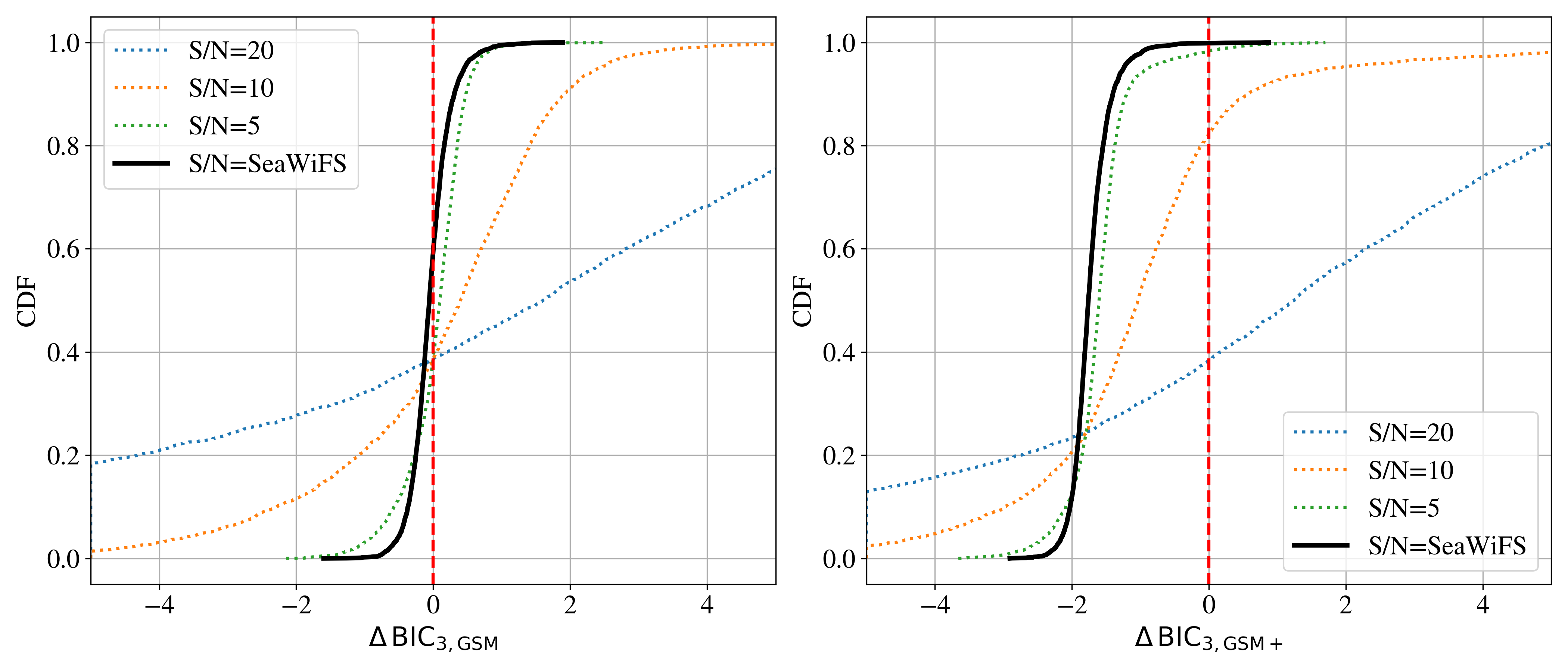
Figure 12 shows distributions for two “GSM” models which also have a fixed exponential but with an even steeper slope (=0.0206) and a power-law for with fixed exponent =1.0337 (GSM) or letting be free (GSM+). Therefore, these are also =3 and =4 models with the same parameters as GIOP and GIOP+. We find that this mode is favored over the model for only 33% of the L23 dataset. Similar to the GIOP model, we show in Supp 6.6 that its retrievals are both highly biased and uncertain.
6.6 Treatment of
The previous section introduced the GSM and GIOP models which adopt fixed shape parameters for the exponential term in . We now examine that choice in the context of the L23 dataset and then consider the consequences for retrievals in the following sub-section.
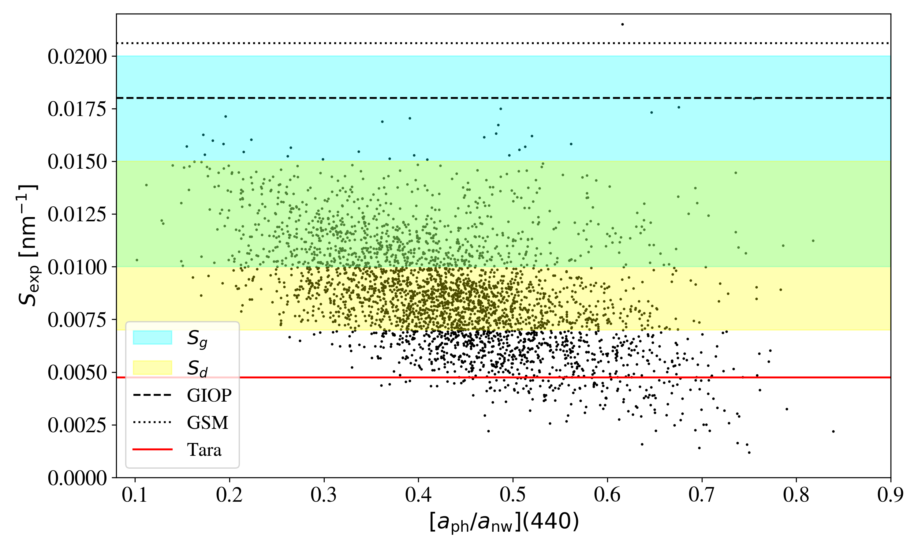
For our fiducial treatment of the exponential component in (Equation 7), the only constraint placed on the shape parameter was that it be positive-definite (). Let us scrutinize that prior as it affects the potential to retrieve phytoplankton and any other constituents (see the previous section). Figure 13 shows the values derived with the model (no phytoplankton) against the fraction of non-water absorption associated with phytoplankton at 440 nm in the L23 spectra, /. The two quantities are anti-correlated because the increased presence of phytoplankton relative to CDOM and detritus tends to give a shallower, non-water absorption spectrum.
We find, as anticipated, that the majority of retrieved values lie within the loci of shape parameters assumed by L23 for CDOM and detritus based on (Lee, \APACyear2006). There is, however, a non-negligible set of retrieved values that are lower than the lowest value assumed by L23; these are partially due to strong phytoplankton absorption. If one were to adopt a stricter prior on than , therefore, one may find statistical evidence for phytoplankton absorption (formally, a distinct component from the best-fit exponential). Indeed, we found this to be the case for the GIOP and GSM models (Figures 11,12) although it is now apparent from Figure 13 that their choices for lie at the upper end of values measured in the ocean (GIOP) or even beyond (GSM). This was by intentional for GSM (Maritorena \BBA Siegel, \APACyear2005), as its designers derived fixed values for and by achieving best retrievals when compared against in-situ data. However, their treatment of errors may not have been well suited to actual SeaWiFS uncertainties (Table 2) and we show below that the model is both biased and yields highly uncertain estimates (in fact, primarily upper limits).


6.7 Retrievals from GSM and GIOP
While the results in Figure 11 and 12 lend support that the GSM and GIOP models as designed may yield a positive detection of , it is important to appreciate the limitations. Consider first individual fits. Figures 14 and 15 show BING analyses on a representative spectrum from L23 (index=170) for GIOP with MODIS observations and GSM on SeaWiFS. It is evident that the algorithm yields only an upper limit in and that the estimates of and are highly uncertain. One notes the large uncertainties and the (weak) degeneracies between the parameters. Therefore, while one retrieves a non-zero, best-estimate for , =10-4 nm-1 is contained within the 90% confidence interval.
We then performed a new set of inferences on the entire L23 dataset assuming MODIS and SeaWiFS simulated spectra for the GIOP and GSM models respectively. In both cases, we calculated from Equations 1 and 3 and performed the inversion with the same model and without perturbing the values due to the presence of noise. The retrievals are presented in Figures 16 and 17. In the second, more realistic case, we perturbed the by the noise model for each satellite (Tables 2, 1), and present these in Figures 18 and 19. Clearly, the retrievals of and are highly uncertain at all values, with nearly two orders of magnitude of scatter. Therefore, the detection of , if it were possible with multi-spectral observations, would be highly uncertain.
The constraints inherent in inversion algorithms like GSM and GIOP do affect the confidence in interpreting changes in maps of retrieved variables such as chlorophyll concentration, absorption coefficients, and backscattering coefficients. The spectral ambiguity in data can lead to changes influenced by variations in other optical properties not fully addressed by the models, making it difficult to attribute changes solely to biological factors. Moreover, the interdependence of retrieved parameters, such as chlorophyll, , and , means that errors in one can propagate to others, complicating the interpretation of these maps. For example, inaccuracies in backscatter coefficient estimates can affect chlorophyll retrievals. Additionally, variability in environmental conditions can impact the accuracy of the retrieved variables. Algorithm performance may vary across different water types and regions, necessitating further caution in interpreting these changes.
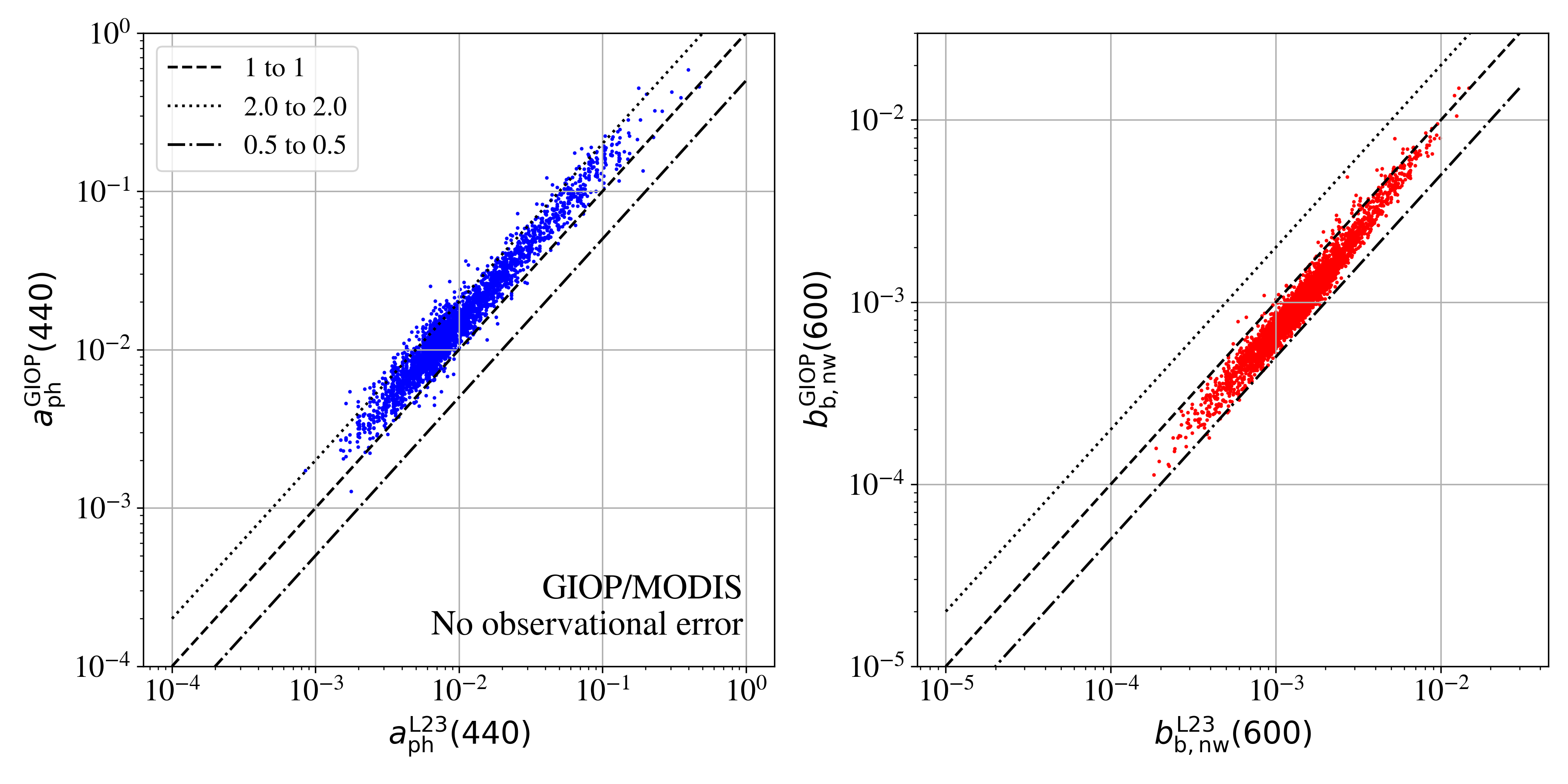
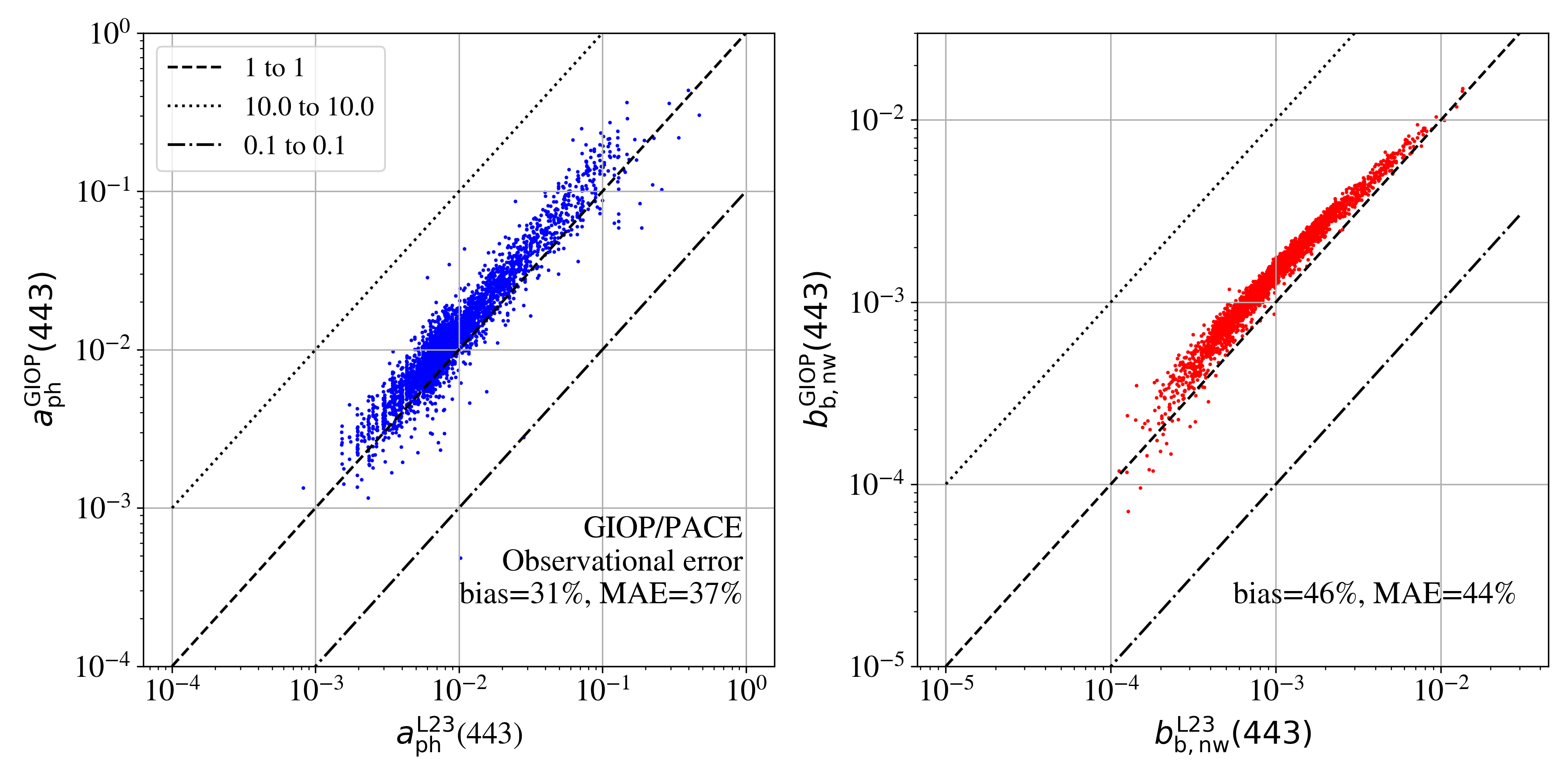
We have also performed retrievals with GIOP on simulated PACE spectra using the uncertainties described in Figure 5. In contrast to the results from simulated MODIS spectra (Figure 18, the retrieved and values have much reduced errors (formally, . However, each set of estimations is biased high by several tens percent and the mean absolute error (MAE) exceeds the PACE requirements (Cetinić \BOthers., \APACyear2018). One could, of course, reduce the bias with one of several post hoc corrections (e.g. modify the value), but this may have other, unanticipated consequences. Furthermore, we reemphasize that our analysis assumes no errors in the radiative transfer, and no uncertainties related to spatial inhomogeneity (among other issues). At present, we believe that PACE is not achieving one or more Level 1 scientific requirements (Cetinić \BOthers., \APACyear2018) and we are pessimistic that these may be met without including strong and strict priors from other datasets in addition to an entirely revamped methodology.
6.8 Previous Assessments
Results from tests of IOP retrieval models have been presented in multiple publications over the years since the beginning of their development (e.g. Mouw \BOthers., \APACyear2017; Werdell \BOthers., \APACyear2018; Seegers \BOthers., \APACyear2018), and a discussion of all of these lies beyond the scope of this manuscript. Nevertheless, we wish to highlight one, in-depth effort summarized by the IOCCG Report 5 (Lee, \APACyear2006). Similar to our work, the participants applied their IOP retrieval algorithms to a simulated (i.e. known) dataset to assess performance. The majority of these algorithms assumed an exponential term for CDOM/detritus absorption with fixed and a steep value (). Similar to the results we found for GIOP and GSM (Figure 17,16), these consistently over-estimated at 440 nm.
Only one team (Boss & Roesler) allowed to vary (from 0.008 to 0.023 ) in their algorithm which followed from the Roesler \BOthers. (\APACyear1989) publication. Referring to their Figure 8.1, one notes less biased values than the other algorithms and that they were the only group to include an error estimation. Given the axes are a log-scaling, one might miss that the uncertainties in are large enough to be consistent with zero. In other words, the results from the only algorithm of the report adopting as a free parameter showed could not be positively detected from simulated data.
6.9 New Methods for Hyperspectral Data
In the context of advancing ocean color remote sensing and PACE, new algorithms have been introduced to enhance the retrieval of phytoplankton pigments using hyperspectral reflectance data (Chase \BOthers., \APACyear2017; Kramer \BOthers., \APACyear2022). However, these approaches face significant challenges due to the fundamental issue of depending primarily on the ratio of backscattering to absorption (/) rather than on these parameters individually as emphasize in the present study. This intrinsic degeneracy means that remote sensing reflectance alone cannot independently determine the absolute values of arbitrary non-water IOPs.
Chase \BOthers. (\APACyear2017) employ an inversion algorithm to estimate phytoplankton pigments by using the spectral shape of reflectance. Their method relies heavily on covariation relationships between chlorophyll-a and accessory pigments, which does not resolve the degeneracy problem but instead depends on pre-established statistical correlations. Furthermore, their analysis of spectral residuals shows no strong relationship between residuals and pigments, underscoring the difficulty of extracting specific pigment information from hyperspectral reflectance alone. Related, our own experiments implementing Gaussian fits to absorption spectra reveal major, insurmountable degeneracies between the components (Prochaska, \APACyear2024).
Similarly, Kramer \BOthers. (\APACyear2022) use principal components regression (PCR) modeling of the second derivative of residuals to reconstruct pigment concentrations from hyperspectral data. While they claim success in modeling multiple pigments, their approach remains fundamentally limited by the same degeneracy issue. The PCR method reduces dimensionality and identifies patterns in the data, yet it still relies on the representativeness of the training dataset and may not generalize well across diverse environmental conditions. Moreover, the requirement for high spectral resolution indicates that the model’s robustness is contingent on specific sensor capabilities and noise levels, further limiting practical applications without extensive a priori data. Indeed, our experiments on derivatives of reveal the uncertainties of the second derivative generally exceed the signal at all wavelengths (Prochaska, \APACyear2024).
These studies, despite their contributions, illustrate the inherent limitations of using for detailed pigment retrieval without strong a priori knowledge or assumptions. Our analysis underscores the necessity of such priors to achieve accurate IOP retrievals, as alone cannot provide unique solutions due to its dependence on the ratio. Therefore, while the advancements by Chase \BOthers. (\APACyear2017) and Kramer \BOthers. (\APACyear2022) are noteworthy, their methodologies should be viewed within the context of these fundamental constraints, highlighting the need for continued refinement and incorporation of comprehensive a priori information in ocean color remote sensing algorithms.
Acknowledgements.
The authors wish to thank B. Ménard, E. Boss, S. Kramer, A. Windle, H. Housekeeper, M. Zhang, and C. Mobley for discussions and/or their input on an earlier draft. We also benefited from conversations with The Astros. Last, we acknowledge deriving new insight on the problem from conversations with M. Kehrli.References
- Behrenfeld \BOthers. (\APACyear2016) \APACinsertmetastarbehrenfeld2016{APACrefauthors}Behrenfeld, M\BPBIJ., O’Malley, R\BPBIT., Boss, E\BPBIS., Westberry, T\BPBIK., Graff, J\BPBIR., Halsey, K\BPBIH.\BDBLBrown, M\BPBIB. \APACrefYearMonthDay2016\APACmonth03. \BBOQ\APACrefatitleRevaluating ocean warming impacts on global phytoplankton Revaluating ocean warming impacts on global phytoplankton.\BBCQ \APACjournalVolNumPagesNature Climate Change63323-330. {APACrefDOI} 10.1038/nclimate2838 \PrintBackRefs\CurrentBib
- Bentler \BBA Bonett (\APACyear1980) \APACinsertmetastarBentler1980{APACrefauthors}Bentler, P\BPBIM.\BCBT \BBA Bonett, D\BPBIG. \APACrefYearMonthDay1980. \BBOQ\APACrefatitleSignificance tests and goodness of fit in the analysis of covariance structures Significance tests and goodness of fit in the analysis of covariance structures.\BBCQ \APACjournalVolNumPagesPsychological Bulletin883588–606. {APACrefDOI} 10.1037/0033-2909.88.3.588 \PrintBackRefs\CurrentBib
- Boss \BOthers. (\APACyear2022) \APACinsertmetastarboss2022{APACrefauthors}Boss, E., Waite, A\BPBIM., Karstensen, J., Trull, T., Muller-Karger, F., Sosik, H\BPBIM.\BDBLWanninkhof, R. \APACrefYearMonthDay2022. \BBOQ\APACrefatitleRecommendations for Plankton Measurements on OceanSITES Moorings With Re levance to Other Observing Sites Recommendations for plankton measurements on oceansites moorings with re levance to other observing sites.\BBCQ \APACjournalVolNumPagesFrontiers in Marine Science9. {APACrefURL} https://www.frontiersin.org/journals/marine-science/articles/10.3389/fmars.2022.929436 {APACrefDOI} 10.3389/fmars.2022.929436 \PrintBackRefs\CurrentBib
- Bricaud \BOthers. (\APACyear1995) \APACinsertmetastarbricaud1995{APACrefauthors}Bricaud, A., Babin, M., Morel, A.\BCBL \BBA Claustre, H. \APACrefYearMonthDay1995\APACmonth07. \BBOQ\APACrefatitleVariability in the chlorophyll-specific absorption coefficients of natural phytoplankton: Analysis and parameterization Variability in the chlorophyll-specific absorption coefficients of natural phytoplankton: Analysis and parameterization.\BBCQ \APACjournalVolNumPagesJournal of Geophysical Research100C713,321-13,332. {APACrefDOI} 10.1029/95JC00463 \PrintBackRefs\CurrentBib
- Bricaud \BOthers. (\APACyear1998) \APACinsertmetastarbricaud1998{APACrefauthors}Bricaud, A., Morel, A., Babin, M., Allali, K.\BCBL \BBA Claustre, H. \APACrefYearMonthDay1998\APACmonth12. \BBOQ\APACrefatitleVariations of light absorption by suspended particles with chlorophyll a concentration in oceanic (case 1) waters: Analysis and implications for bio-optical models Variations of light absorption by suspended particles with chlorophyll a concentration in oceanic (case 1) waters: Analysis and implications for bio-optical models.\BBCQ \APACjournalVolNumPagesJ. Geophys. Res.103C1331,033-31,044. {APACrefDOI} 10.1029/98JC02712 \PrintBackRefs\CurrentBib
- Cael \BOthers. (\APACyear2023) \APACinsertmetastarcael+2023{APACrefauthors}Cael, B\BPBIB., Bisson, K., Boss, E.\BCBL \BBA Erickson, Z\BPBIr\BPBIK. \APACrefYearMonthDay2023. \BBOQ\APACrefatitleHow many independent quantities can be extracted from ocean color? How many independent quantities can be extracted from ocean color?\BBCQ \APACjournalVolNumPagesLimnology and Oceanography Letters84603-610. {APACrefURL} https://aslopubs.onlinelibrary.wiley.com/doi/abs/10.1002/lol2.10319 {APACrefDOI} https://doi.org/10.1002/lol2.10319 \PrintBackRefs\CurrentBib
- Cetinić \BOthers. (\APACyear2018) \APACinsertmetastarPACE_tech_vol6{APACrefauthors}Cetinić, I., McClain, C\BPBIR.\BCBL \BBA Werdell, P\BPBIJ. \APACrefYearMonthDay2018. \APACrefbtitlePACE Technical Report Series, Volume 6: Data Product Requirements and Error Budgets PACE Technical Report Series, Volume 6: Data Product Requirements and Error Budgets \APACbVolEdTRNASA Technical Memorandum \BNUM NASA/TM-2018 - 2018-219027/ Vol. 6. \APACaddressInstitutionGreenbelt, MDNASA Goddard Space Flight Center. \PrintBackRefs\CurrentBib
- Cetinić \BOthers. (\APACyear2024) \APACinsertmetastarcetinic+2024{APACrefauthors}Cetinić, I., Rousseaux, C\BPBIS., Carroll, I\BPBIT., Chase, A\BPBIP\BPBI., Kramer, S\BPBIJ., Werdell, P\BPBIJ.\BDBLSayers, M. \APACrefYearMonthDay2024. \BBOQ\APACrefatitlePhytoplankton composition from sPACE: Requirements, opportunities, and challenges Phytoplankton composition from space: Requirements, opportunities, and challenges.\BBCQ \APACjournalVolNumPagesRemote Sensing of Environment302113964. {APACrefURL} https://www.sciencedirect.com/science/article/pii/S0034425723005163 {APACrefDOI} https://doi.org/10.1016/j.rse.2023.113964 \PrintBackRefs\CurrentBib
- Chase \BOthers. (\APACyear2017) \APACinsertmetastarchase+2017{APACrefauthors}Chase, A\BPBIP., Boss, E., Cetinić, I.\BCBL \BBA Slade, W. \APACrefYearMonthDay2017\APACmonth12. \BBOQ\APACrefatitleEstimation of Phytoplankton Accessory Pigments From Hyperspectral Reflectance Spectra: Toward a Global Algorithm Estimation of Phytoplankton Accessory Pigments From Hyperspectral Reflectance Spectra: Toward a Global Algorithm.\BBCQ \APACjournalVolNumPagesJournal of Geophysical Research (Oceans)122129725-9743. {APACrefDOI} 10.1002/2017JC012859 \PrintBackRefs\CurrentBib
- Cloern \BBA Jassby (\APACyear2010) \APACinsertmetastarCloern2010{APACrefauthors}Cloern, J\BPBIE.\BCBT \BBA Jassby, A\BPBID. \APACrefYearMonthDay2010\APACmonth03. \BBOQ\APACrefatitlePatterns and Scales of Phytoplankton Variability in Estuarine–Coastal Ecosystems Patterns and scales of phytoplankton variability in estuarine–coastal ecosystems.\BBCQ \APACjournalVolNumPagesEstuaries and Coasts332230–241. {APACrefURL} https://doi.org/10.1007/s12237-009-9195-3 {APACrefDOI} 10.1007/s12237-009-9195-3 \PrintBackRefs\CurrentBib
- Defoin-Platel \BBA Chami (\APACyear2007) \APACinsertmetastardefoin2007{APACrefauthors}Defoin-Platel, M.\BCBT \BBA Chami, M. \APACrefYearMonthDay2007\APACmonth03. \BBOQ\APACrefatitleHow ambiguous is the inverse problem of ocean color in coastal waters? How ambiguous is the inverse problem of ocean color in coastal waters?\BBCQ \APACjournalVolNumPagesJournal of Geophysical Research (Oceans)112C3C03004. {APACrefDOI} 10.1029/2006JC003847 \PrintBackRefs\CurrentBib
- Flombaum \BOthers. (\APACyear2020) \APACinsertmetastarflombaum2020{APACrefauthors}Flombaum, P., Wang, W\BHBIL., Primeau, F\BPBIW.\BCBL \BBA Martiny, A\BPBIC. \APACrefYearMonthDay2020\APACmonth01. \BBOQ\APACrefatitleGlobal picophytoplankton niche partitioning predicts overall positive response to ocean warming Global picophytoplankton niche partitioning predicts overall positive response to ocean warming.\BBCQ \APACjournalVolNumPagesNature Geoscience132116-120. {APACrefDOI} 10.1038/s41561-019-0524-2 \PrintBackRefs\CurrentBib
- Foreman-Mackey \BOthers. (\APACyear2013) \APACinsertmetastaremcee{APACrefauthors}Foreman-Mackey, D., Hogg, D\BPBIW., Lang, D.\BCBL \BBA Goodman, J. \APACrefYearMonthDay2013\APACmonth03. \BBOQ\APACrefatitle¡tt¿emcee¡/tt¿: The MCMC Hammer ¡tt¿emcee¡/tt¿: The mcmc hammer.\BBCQ \APACjournalVolNumPagesPublications of the Astronomical Society of the Pacific125925306–312. {APACrefURL} http://dx.doi.org/10.1086/670067 {APACrefDOI} 10.1086/670067 \PrintBackRefs\CurrentBib
- Fox \BOthers. (\APACyear2022) \APACinsertmetastarfox2022{APACrefauthors}Fox, J., Kramer, S\BPBIJ., Graff, J\BPBIR., Behrenfeld, M\BPBIc\BPBIJ., Boss, E., Tilstone, G.\BCBL \BBA Halsey, K\BPBIH. \APACrefYearMonthDay2022. \BBOQ\APACrefatitleAn absorption-based approach to improved estimates of phytoplankton bio mass and net primary production An absorption-based approach to improved estimates of phytoplankton bio mass and net primary production.\BBCQ \APACjournalVolNumPagesLimnology and Oceanography Letters75419-426. {APACrefURL} https://aslopubs.onlinelibrary.wiley.com/doi/abs/10.1002/lol2.10275 {APACrefDOI} https://doi.org/10.1002/lol2.10275 \PrintBackRefs\CurrentBib
- Frouin \BBA Pelletier (\APACyear2015) \APACinsertmetastarfrouin2015{APACrefauthors}Frouin, R.\BCBT \BBA Pelletier, B. \APACrefYearMonthDay2015\APACmonth03. \BBOQ\APACrefatitleBayesian methodology for inverting satellite ocean-color data Bayesian methodology for inverting satellite ocean-color data.\BBCQ \APACjournalVolNumPagesRemote Sensing of Environment159332-360. {APACrefDOI} 10.1016/j.rse.2014.12.001 \PrintBackRefs\CurrentBib
- Garver \BOthers. (\APACyear1994) \APACinsertmetastargarver1994{APACrefauthors}Garver, S\BPBIA., Siegel, D\BPBIA.\BCBL \BBA B. Greg, M. \APACrefYearMonthDay1994\APACmonth09. \BBOQ\APACrefatitleVariability in near-surface particulate absorption spectra: What can a satellite ocean color imager see? Variability in near-surface particulate absorption spectra: What can a satellite ocean color imager see?\BBCQ \APACjournalVolNumPagesLimnology and Oceanography3961349-1367. {APACrefDOI} 10.4319/lo.1994.39.6.1349 \PrintBackRefs\CurrentBib
- Gordon (\APACyear1973) \APACinsertmetastargordon1973{APACrefauthors}Gordon, H\BPBIR. \APACrefYearMonthDay1973\APACmonth12. \BBOQ\APACrefatitleSimple Calculation of the Diffuse Reflectance of the Ocean Simple Calculation of the Diffuse Reflectance of the Ocean.\BBCQ \APACjournalVolNumPagesAppl. Opt.12122803. {APACrefDOI} 10.1364/AO.12.002803 \PrintBackRefs\CurrentBib
- Gordon (\APACyear1986) \APACinsertmetastargordon1986{APACrefauthors}Gordon, H\BPBIR. \APACrefYearMonthDay1986\APACmonth08. \BBOQ\APACrefatitleDistribution Of Irradiance On The Sea Surface Resulting From A Point Source Imbedded In The Ocean Distribution Of Irradiance On The Sea Surface Resulting From A Point Source Imbedded In The Ocean.\BBCQ \BIn \APACrefbtitleSociety of Photo-Optical Instrumentation Engineers (SPIE) Conference Series Society of photo-optical instrumentation engineers (spie) conference series (\BVOL 637, \BPG 66-71). {APACrefDOI} 10.1117/12.964216 \PrintBackRefs\CurrentBib
- Gordon \BBA Morel (\APACyear1983) \APACinsertmetastargordon1983{APACrefauthors}Gordon, H\BPBIR.\BCBT \BBA Morel, A\BPBIY. \APACrefYear1983. \APACrefbtitleRemote Assessment of Ocean Color for Interpretation of Satellite Visible Imagery Remote assessment of ocean color for interpretation of satellite visible imagery (\BVOL 4). \APACaddressPublisherSpringer-Verlag. \APACrefnoteOnline ISBN: 9781118663707 {APACrefDOI} 10.1029/LN004 \PrintBackRefs\CurrentBib
- Hansen (\APACyear1971) \APACinsertmetastarhansen1971{APACrefauthors}Hansen, J\BPBIE. \APACrefYearMonthDay1971\APACmonth11. \BBOQ\APACrefatitleMultiple Scattering of Polarized Light in Planetary Atmospheres Part II. Sunlight Reflected by Terrestrial Water Clouds. Multiple Scattering of Polarized Light in Planetary Atmospheres Part II. Sunlight Reflected by Terrestrial Water Clouds.\BBCQ \APACjournalVolNumPagesJournal of the Atmospheric Sciences2881400-1426. {APACrefDOI} 10.1175/1520-0469(1971)028¡1400:MSOPLI¿2.0.CO;2 \PrintBackRefs\CurrentBib
- Hooker \BOthers. (\APACyear2020) \APACinsertmetastarhooker2020{APACrefauthors}Hooker, S\BPBIB., Matsuoka, A., Kudela, R\BPBIM., Yamashita, Y., Suzuki, K.\BCBL \BBA Houskeeper, H\BPBIF. \APACrefYearMonthDay2020\APACmonth01. \BBOQ\APACrefatitleA global end-member approach to derive aCDOM(440) from near-surface optical measurements A global end-member approach to derive aCDOM(440) from near-surface optical measurements.\BBCQ \APACjournalVolNumPagesBiogeosciences172475-497. {APACrefDOI} 10.5194/bg-17-475-2020 \PrintBackRefs\CurrentBib
- Hovis \BOthers. (\APACyear1980) \APACinsertmetastarHovis1980{APACrefauthors}Hovis, W\BPBIA., Clark, D\BPBIK., Anderson, F., Austin, R\BPBIW., Wilson, W\BPBIH., Baker, E\BPBIT.\BDBLYentsch, C\BPBIS. \APACrefYearMonthDay1980\APACmonth103. \BBOQ\APACrefatitleNimbus-7 Coastal Zone Color Scanner: System Description and Initial Imagery Nimbus-7 coastal zone color scanner: System description and initial imagery.\BBCQ \APACjournalVolNumPagesScience210446560–63. {APACrefDOI} 10.1126/science.210.4465.60 \PrintBackRefs\CurrentBib
- Kramer \BOthers. (\APACyear2022) \APACinsertmetastarkramer2022{APACrefauthors}Kramer, S\BPBIJ., Siegel, D\BPBIA., Maritorena, S.\BCBL \BBA Catlett, D. \APACrefYearMonthDay2022\APACmonth03. \BBOQ\APACrefatitleModeling surface ocean phytoplankton pigments from hyperspectral remote sensing reflectance on global scales Modeling surface ocean phytoplankton pigments from hyperspectral remote sensing reflectance on global scales.\BBCQ \APACjournalVolNumPagesRemote Sensing of Environment270112879. {APACrefDOI} 10.1016/j.rse.2021.112879 \PrintBackRefs\CurrentBib
- Kudela \BOthers. (\APACyear2019) \APACinsertmetastarkudela2019{APACrefauthors}Kudela, R\BPBIM., Hooker, S\BPBIB., Houskeeper, H\BPBIF.\BCBL \BBA McPherson, M. \APACrefYearMonthDay2019\APACmonth09. \BBOQ\APACrefatitleThe Influence of Signal to Noise Ratio of Legacy Airborne and Satellite Sensors for Simulating Next-Generation Coastal and Inland Water Products The Influence of Signal to Noise Ratio of Legacy Airborne and Satellite Sensors for Simulating Next-Generation Coastal and Inland Water Products.\BBCQ \APACjournalVolNumPagesRemote Sensing11182071. {APACrefDOI} 10.3390/rs11182071 \PrintBackRefs\CurrentBib
- Lee (\APACyear2006) \APACinsertmetastarIOCCG2006{APACrefauthors}Lee, Z. \APACrefYearMonthDay2006. \APACrefbtitleRemote Sensing of Inherent Optical Properties: Fundamentals, Tests of Algorithms, and Applications Remote sensing of inherent optical properties: Fundamentals, tests of algorithms, and applications \APACbVolEdTRIOCCG Report \BNUM 5. \APACaddressInstitutionDartmouth, CanadaInternational Ocean-Colour Coordinating Group (IOCCG). \APACrefnoteAn Affiliated Program of the Scientific Committee on Oceanic Research (SCOR) and An Associate Member of the Committee on Earth Observation Satellites (CEOS) \PrintBackRefs\CurrentBib
- Lee \BOthers. (\APACyear2002) \APACinsertmetastarlee+2002{APACrefauthors}Lee, Z., Carder, K\BPBIL.\BCBL \BBA Arnone, R\BPBIA. \APACrefYearMonthDay2002\APACmonth09. \BBOQ\APACrefatitleDeriving inherent optical properties from water color: a multiband quasi-analytical algorithm for optically deep waters Deriving inherent optical properties from water color: a multiband quasi-analytical algorithm for optically deep waters.\BBCQ \APACjournalVolNumPagesAppl. Opt.41275755-5772. {APACrefDOI} 10.1364/AO.41.005755 \PrintBackRefs\CurrentBib
- Lee \BOthers. (\APACyear2002) \APACinsertmetastarLee2002{APACrefauthors}Lee, Z., Carder, K\BPBIL.\BCBL \BBA Arnone, R\BPBIA. \APACrefYearMonthDay2002Sep. \BBOQ\APACrefatitleDeriving inherent optical properties from water color: a multiband qua si-analytical algorithm for optically deep waters Deriving inherent optical properties from water color: a multiband qua si-analytical algorithm for optically deep waters.\BBCQ \APACjournalVolNumPagesAppl. Opt.41275755–5772. {APACrefURL} https://opg.optica.org/ao/abstract.cfm?URI=ao-41-27-5755 {APACrefDOI} 10.1364/AO.41.005755 \PrintBackRefs\CurrentBib
- Loisel \BOthers. (\APACyear2023) \APACinsertmetastarloisel23{APACrefauthors}Loisel, H., Schaffer Ferreira Jorge, D., Reynolds, R\BPBIA.\BCBL \BBA Stramski, D. \APACrefYearMonthDay2023\APACmonth08. \BBOQ\APACrefatitleA synthetic optical database generated by radiative transfer simulations in support of studies in ocean optics and optical remote sensing of the global ocean A synthetic optical database generated by radiative transfer simulations in support of studies in ocean optics and optical remote sensing of the global ocean.\BBCQ \APACjournalVolNumPagesEarth System Science Data1583711-3731. {APACrefDOI} 10.5194/essd-15-3711-2023 \PrintBackRefs\CurrentBib
- Loisel \BBA Stramski (\APACyear2000) \APACinsertmetastarls1{APACrefauthors}Loisel, H.\BCBT \BBA Stramski, D. \APACrefYearMonthDay2000\APACmonth06. \BBOQ\APACrefatitleEstimation of the Inherent Optical Properties of Natural Waters from the Irradiance Attenuation Coefficient and Reflectance in the Presence of Raman Scattering Estimation of the Inherent Optical Properties of Natural Waters from the Irradiance Attenuation Coefficient and Reflectance in the Presence of Raman Scattering.\BBCQ \APACjournalVolNumPagesAppl. Opt.39183001-3011. {APACrefDOI} 10.1364/AO.39.003001 \PrintBackRefs\CurrentBib
- Loisel \BOthers. (\APACyear2018) \APACinsertmetastarls2{APACrefauthors}Loisel, H., Stramski, D., Dessailly, D., Jamet, C., Li, L.\BCBL \BBA Reynolds, R\BPBIA. \APACrefYearMonthDay2018\APACmonth03. \BBOQ\APACrefatitleAn Inverse Model for Estimating the Optical Absorption and Backscattering Coefficients of Seawater From Remote-Sensing Reflectance Over a Broad Range of Oceanic and Coastal Marine Environments An Inverse Model for Estimating the Optical Absorption and Backscattering Coefficients of Seawater From Remote-Sensing Reflectance Over a Broad Range of Oceanic and Coastal Marine Environments.\BBCQ \APACjournalVolNumPagesJournal of Geophysical Research (Oceans)12332141-2171. {APACrefDOI} 10.1002/2017JC013632 \PrintBackRefs\CurrentBib
- Maritorena \BBA Siegel (\APACyear2005) \APACinsertmetastarmaritorena2005{APACrefauthors}Maritorena, S.\BCBT \BBA Siegel, D\BPBIA. \APACrefYearMonthDay2005\APACmonth02. \BBOQ\APACrefatitleConsistent merging of satellite ocean color data sets using a bio-optical model Consistent merging of satellite ocean color data sets using a bio-optical model.\BBCQ \APACjournalVolNumPagesRemote Sensing of Environment944429-440. {APACrefDOI} 10.1016/j.rse.2004.08.014 \PrintBackRefs\CurrentBib
- Maritorena \BOthers. (\APACyear2002) \APACinsertmetastarmaritorena2002{APACrefauthors}Maritorena, S., Siegel, D\BPBIA.\BCBL \BBA Peterson, A\BPBIR. \APACrefYearMonthDay2002\APACmonth05. \BBOQ\APACrefatitleOptimization of a semianalytical ocean color model for global-scale applications Optimization of a semianalytical ocean color model for global-scale applications.\BBCQ \APACjournalVolNumPagesAppl. Opt.41152705-2714. {APACrefDOI} 10.1364/AO.41.002705 \PrintBackRefs\CurrentBib
- Mason \BOthers. (\APACyear2016) \APACinsertmetastarMason2016{APACrefauthors}Mason, J\BPBID., Cone, M\BPBIT.\BCBL \BBA Fry, E\BPBIS. \APACrefYearMonthDay2016Sep. \BBOQ\APACrefatitleUltraviolet (250–550  nm) absorption spectrum of pu re water Ultraviolet (250–550  nm) absorption spectrum of pu re water.\BBCQ \APACjournalVolNumPagesAppl. Opt.55257163–7172. {APACrefURL} https://opg.optica.org/ao/abstract.cfm?URI=ao-55-25-7163 {APACrefDOI} 10.1364/AO.55.007163 \PrintBackRefs\CurrentBib
- C\BPBID. Mobley \BBA Sundman (\APACyear2013) \APACinsertmetastarhydrolight{APACrefauthors}Mobley, C\BPBID.\BCBT \BBA Sundman, L\BPBIK. \APACrefYearMonthDay2013. \APACrefbtitleHydrolight 5.2 Ecolight 5.2 Users’ Guide Hydrolight 5.2 ecolight 5.2 users’ guide \APACbVolEdTR\BTR. \APACaddressInstitutionSequoia Scientific, Inc. {APACrefURL} https://www.sequoiasci.com/wp-content/uploads/2013/07/HE52UsersGuide.pdf \PrintBackRefs\CurrentBib
- C\BPBID\BPBIe. Mobley (\APACyear2022) \APACinsertmetastarMobley2022{APACrefauthors}Mobley, C\BPBID\BPBIe. \APACrefYear2022. \APACrefbtitleThe Oceanic Optics Book The oceanic optics book. \APACaddressPublisherDartmouth, NS, CanadaInternational Ocean Colour Coordinating Group (IOCCG). {APACrefDOI} http://dx.doi.org/10.25607/OBP-1710 \PrintBackRefs\CurrentBib
- Mouw \BOthers. (\APACyear2017) \APACinsertmetastarmouw+2017{APACrefauthors}Mouw, C\BPBIB., Hardman-Mountford, N\BPBIJ., Alvain, S., Bracher, A., Brewin, R\BPBIJ\BPBIW., Bricaud, A.\BDBLUitz, J\BPBIi. \APACrefYearMonthDay2017. \BBOQ\APACrefatitleA Consumer’s Guide to Satellite Remote Sensing of Multiple Phytoplankton Groups in the Global Ocean A consumer’s guide to satellite remote sensing of multiple phytoplankton groups in the global ocean.\BBCQ \APACjournalVolNumPagesFrontiers in Marine Science4. {APACrefURL} https://www.frontiersin.org/journals/marine-science/articles/10.3389/fmars.2017.00041 {APACrefDOI} 10.3389/fmars.2017.00041 \PrintBackRefs\CurrentBib
- SeaBASS (\APACyear2024) \APACinsertmetastarmodis_matchup{APACrefauthors}NASA Goddard Space Flight Center. \APACrefYearMonthDay2024. \APACrefbtitleSeaBASS Validation Search. Seabass validation search. \APAChowpublishedhttps://seabass.gsfc.nasa.gov/search/?search_type=Perform%20Validation%20Search&val_sata=1&val_products=11&val_source=0. \APACrefnoteAccessed: 2024-06 \PrintBackRefs\CurrentBib
- Prochaska (\APACyear2024) \APACinsertmetastarbing_doi{APACrefauthors}Prochaska, J\BPBIX. \APACrefYearMonthDay2024\APACmonth01. \APACrefbtitleocean-colour/bing: Submitted to Nature Comm. ocean-colour/bing: Submitted to Nature Comm. \APACaddressPublisherZenodo. {APACrefURL} https://doi.org/10.5281/zenodo.13292701 {APACrefDOI} 10.5281/zenodo.13292701 \PrintBackRefs\CurrentBib
- Prochaska \BBA Gray (\APACyear2024) \APACinsertmetastarpg2024{APACrefauthors}Prochaska, J\BPBIX.\BCBT \BBA Gray, P. \APACrefYearMonthDay2024\APACmonth06. \BBOQ\APACrefatitleOn the Fundamental Additive Modes of Ocean Color Absorption On the fundamental additive modes of ocean color absorption.\BBCQ \APACjournalVolNumPagesLimnology & Oceanography. {APACrefURL} http://dx.doi.org/10.22541/essoar.171828481.15444713/v1 {APACrefDOI} 10.22541/essoar.171828481.15444713/v1 \PrintBackRefs\CurrentBib
- Roesler \BOthers. (\APACyear1989) \APACinsertmetastarroesler1989{APACrefauthors}Roesler, C\BPBIS., Perry, M\BPBIJ.\BCBL \BBA Carder, K\BPBIL. \APACrefYearMonthDay1989\APACmonth12. \BBOQ\APACrefatitleModeling in situ phytoplankton absorption from total absorption spectra in productive inland marine waters Modeling in situ phytoplankton absorption from total absorption spectra in productive inland marine waters.\BBCQ \APACjournalVolNumPagesLimnology and Oceanography3481510-1523. {APACrefDOI} 10.4319/lo.1989.34.8.1510 \PrintBackRefs\CurrentBib
- Seegers \BOthers. (\APACyear2018) \APACinsertmetastarseegers+2018{APACrefauthors}Seegers, B\BPBIN., Stumpf, R\BPBIP., Schaeffer, B\BPBIA., Loftin, K\BPBIA.\BCBL \BBA Werdell, P\BPBIJ. \APACrefYearMonthDay2018\APACmonth03. \BBOQ\APACrefatitlePerformance metrics for the assessment of satellite data products: an ocean color case study Performance metrics for the assessment of satellite data products: an ocean color case study.\BBCQ \APACjournalVolNumPagesOptics Express2667404. {APACrefDOI} 10.1364/OE.26.007404 \PrintBackRefs\CurrentBib
- Siegel \BOthers. (\APACyear2013) \APACinsertmetastarsiegel2013{APACrefauthors}Siegel, D\BPBIA., Behrenfeld, M\BPBIJ., Maritorena, S., McClain, C\BPBIR., Antoine, D., Bailey, S\BPBIW.\BDBLYoder, J\BPBIA. \APACrefYearMonthDay2013\APACmonth08. \BBOQ\APACrefatitleRegional to global assessments of phytoplankton dynamics from the SeaWiFS mission Regional to global assessments of phytoplankton dynamics from the SeaWiFS mission.\BBCQ \APACjournalVolNumPagesRemote Sensing of Environment13577-91. {APACrefDOI} 10.1016/j.rse.2013.03.025 \PrintBackRefs\CurrentBib
- Stramski \BOthers. (\APACyear2001) \APACinsertmetastarstramski2001{APACrefauthors}Stramski, D., Bricaud, A.\BCBL \BBA Morel, A. \APACrefYearMonthDay2001\APACmonth06. \BBOQ\APACrefatitleModeling the Inherent Optical Properties of the Ocean Based on the Detailed Composition of the Planktonic Community Modeling the Inherent Optical Properties of the Ocean Based on the Detailed Composition of the Planktonic Community.\BBCQ \APACjournalVolNumPagesAppl. Opt.40182929-2945. {APACrefDOI} 10.1364/AO.40.002929 \PrintBackRefs\CurrentBib
- Stramski \BOthers. (\APACyear2022) \APACinsertmetastarpoc{APACrefauthors}Stramski, D., Joshi, I.\BCBL \BBA Reynolds, R\BPBIA. \APACrefYearMonthDay2022\APACmonth02. \BBOQ\APACrefatitleOcean color algorithms to estimate the concentration of particulate organic carbon in surface waters of the global ocean in support of a long-term data record from multiple satellite missions Ocean color algorithms to estimate the concentration of particulate organic carbon in surface waters of the global ocean in support of a long-term data record from multiple satellite missions.\BBCQ \APACjournalVolNumPagesRemote Sensing of Environment269112776. {APACrefDOI} 10.1016/j.rse.2021.112776 \PrintBackRefs\CurrentBib
- Sydor \BOthers. (\APACyear2004) \APACinsertmetastarsydor2004{APACrefauthors}Sydor, M., Gould, R\BPBIW., Arnone, R\BPBIA., Haltrin, V\BPBII.\BCBL \BBA Goode, W. \APACrefYearMonthDay2004\APACmonth04. \BBOQ\APACrefatitleUniqueness in Remote Sensing of the Inherent Optical Properties of Ocean Water Uniqueness in Remote Sensing of the Inherent Optical Properties of Ocean Water.\BBCQ \APACjournalVolNumPagesAppl. Opt.43102156-2162. {APACrefDOI} 10.1364/AO.43.002156 \PrintBackRefs\CurrentBib
- Twardowski \BOthers. (\APACyear2018) \APACinsertmetastartwardowski2018{APACrefauthors}Twardowski, M\BPBIS., Jamet, C.\BCBL \BBA Loisel, H. \APACrefYearMonthDay2018\APACmonth05. \BBOQ\APACrefatitleAnalytical model to derive suspended particulate matter concentration in natural waters by inversion of optical attenuation and backscattering Analytical model to derive suspended particulate matter concentration in natural waters by inversion of optical attenuation and backscattering.\BBCQ \BIn W\BPBIW. Hou \BBA R\BPBIA. Arnone (\BEDS), \APACrefbtitleOcean Sensing and Monitoring X Ocean sensing and monitoring x (\BVOL 10631, \BPG 106310H). {APACrefDOI} 10.1117/12.2309995 \PrintBackRefs\CurrentBib
- Werdell \BBA Bailey (\APACyear2002) \APACinsertmetastarseabass{APACrefauthors}Werdell, P\BPBIJ.\BCBT \BBA Bailey, S\BPBIW. \APACrefYearMonthDay2002. \APACrefbtitleThe SeaWiFS Bio-optical Archive and Storage System (SeaBASS): Current architecture and implementation The SeaWiFS bio-optical archive and storage system (SeaBASS): Current architecture and implementation \APACbVolEdTRNASA Tech. Memo. \BNUM 2002-211617. \APACaddressInstitutionGreenbelt, MarylandNASA Goddard Space Flight Center. \PrintBackRefs\CurrentBib
- Werdell \BOthers. (\APACyear2013) \APACinsertmetastarwerdell2013{APACrefauthors}Werdell, P\BPBIJ., Franz, B\BPBIA., Bailey, S\BPBIW., Feldman, G\BPBIC., Boss, E., Brando, V\BPBIE.\BDBLMangin, A. \APACrefYearMonthDay2013\APACmonth04. \BBOQ\APACrefatitleGeneralized ocean color inversion model for retrieving marine inherent optical properties Generalized ocean color inversion model for retrieving marine inherent optical properties.\BBCQ \APACjournalVolNumPagesApplied Optics52102019. {APACrefDOI} 10.1364/AO.52.002019 \PrintBackRefs\CurrentBib
- Werdell \BOthers. (\APACyear2018) \APACinsertmetastarwerdell2018{APACrefauthors}Werdell, P\BPBIJ., McKinna, L\BPBII\BPBIW., Boss, E., Ackleson, S\BPBIG., Craig, S\BPBIE., Gregg, W\BPBIW.\BDBLZhang, X. \APACrefYearMonthDay2018\APACmonth01. \BBOQ\APACrefatitleAn overview of approaches and challenges for retrieving marine inherent optical properties from ocean color remote sensing An overview of approaches and challenges for retrieving marine inherent optical properties from ocean color remote sensing.\BBCQ \APACjournalVolNumPagesProgress in Oceanography160186-212. {APACrefDOI} 10.1016/j.pocean.2018.01.001 \PrintBackRefs\CurrentBib
- Wolanin \BOthers. (\APACyear2015) \APACinsertmetastarwolanin2015{APACrefauthors}Wolanin, A., Rozanov, V\BPBIV., Dinter, T., Noël, S., Vountas, M., Burrows, J\BPBIP.\BCBL \BBA Bracher, A. \APACrefYearMonthDay2015\APACmonth09. \BBOQ\APACrefatitleGlobal retrieval of marine and terrestrial chlorophyll fluorescence at its red peak using hyperspectral top of atmosphere radiance measurements: Feasibility study and first results Global retrieval of marine and terrestrial chlorophyll fluorescence at its red peak using hyperspectral top of atmosphere radiance measurements: Feasibility study and first results.\BBCQ \APACjournalVolNumPagesRemote Sensing of Environment166243-261. {APACrefDOI} 10.1016/j.rse.2015.05.018 \PrintBackRefs\CurrentBib
- Zege \BOthers. (\APACyear1991) \APACinsertmetastarZege1991{APACrefauthors}Zege, E\BPBIP., Ivanov, A\BPBIP.\BCBL \BBA Katsev, I\BPBIL. \APACrefYear1991. \APACrefbtitleImage Transfer Through a Scattering Medium Image transfer through a scattering medium. \APACaddressPublisherSpringer-Verlag. \PrintBackRefs\CurrentBib
- Zhang \BOthers. (\APACyear2022) \APACinsertmetastarZhang2022{APACrefauthors}Zhang, M., Ibrahim, A., Franz, B\BPBIA.\BCBL \BBA a nd Andrew M. Sayer, Z\BPBIA. \APACrefYearMonthDay2022Aug. \BBOQ\APACrefatitleEstimating pixel-level uncertainty in ocean color retrievals from MODI S Estimating pixel-level uncertainty in ocean color retrievals from modi s.\BBCQ \APACjournalVolNumPagesOpt. Express301731415–31438. {APACrefURL} https://opg.optica.org/oe/abstract.cfm?URI=oe-30-17-31415 {APACrefDOI} 10.1364/OE.460735 \PrintBackRefs\CurrentBib