An anisotropic, brittle damage model for finite strains with a generic damage tensor regularization

Abstract. This paper establishes a universal framework for the nonlocal modeling of anisotropic damage at finite strains. By the combination of two recent works, the new framework allows for the flexible incorporation of different established hyperelastic finite strain material formulations into anisotropic damage whilst ensuring mesh-independent results by employing a generic set of micromorphic gradient-extensions. First, the anisotropic damage model, generally satisfying the damage growth criterion, is investigated for the specific choice of a Neo-Hookean material on a single element. Next, the model is applied with different gradient-extensions in structural simulations of an asymmetrically notched specimen to identify an efficient choice in the form of a volumetric-deviatoric regularization. Thereafter, the universal framework, which is without loss of generality here specified for a Neo-Hookean material with a volumetric-deviatoric gradient-extension, successfully serves for the complex simulation of a pressure loaded rotor blade.

After acceptance of the manuscript, we make the codes of the material subroutines accessible to the public at https://doi.org/10.5281/zenodo.11171630.

Keywords: Anisotropic damage, finite strains, gradient-extension

1 Introduction

Motivation.  The prediction of structural failure requires the precise local modeling of damage and the accurate nonlocal regularization of the softening phenomenon in structural simulations. Both aspects, the modeling and regularization of softening due to damage, constitute fundamental fields of research in continuum mechanics that continuously generate enhanced local and nonlocal solutions. This motivates the proposition of a general modeling framework that combines a flexible local anisotropic damage model with different nonlocal gradient-extensions in this work. The following paragraphs only provide an overview of recent contributions to both fields. For a general overview on damage modeling, we refer to the works of e.g. Lemaitre and Desmorat [2005], Voyiadjis and Kattan [2009], Besson [2010], and Murakami [2012].

Modeling of softening.  Mattiello and Desmorat [2021] investigate different evolution laws for symmetric second-order damage tensors with respect to the Lode angle dependency. Dorn and Wulfinghoff [2021] assume a multiplicative decomposition of the deformation gradient into normal and shear crack contributions that directly yields a tension-compression asymmetry. For low cycle fatigue, Ferreira et al. [2022] propose a damage evolution law depending on the stress triaxiality and test the model in material point studies for multiaxial and nonproportional loading paths. In Reese et al. [2021], a local formulation for anisotropic damage is introduced that can incorporate arbitrary hyperelastic energies and generally fulfills the damage growth criterion (Wulfinghoff et al. [2017]). Petrini et al. [2023] use a dynamic phase-field model with a fourth-order degradation tensor to account for damage anisotropy at infinitesimal strains. Based on the work by Voyiadjis and Kattan [2017] and Basaran [2023], Voyiadjis and Kattan [2024] present an unsymmetrical decomposition of the tensorial damage variable to separately account for crack and void induced damage. To capture stiffness recovery after damage evolution, Shojaei and Voyiadjis [2023] lay the theoretical groundwork for statistical continuum damage healing mechanics by considering the sealing and healing effects. Loiseau et al. [2023] employ a data-driven approach to identify an accurate tensorial representation of anisotropic damage to account for micro-cracking based on a virtual set of beam-particle simulations.

Regularization of softening.  Jirásek and Desmorat [2019] investigate the regularization performance of a new nonlocal integral approach with a damage-dependent interaction distance for pure damage models, damage-plasticity models, and damage with inelastic strain models. Ahmed et al. [2021] present a damage model for concrete that captures tensile, compressive, and shear damage with separate scalar damage variables, where each quantity is regularized by a gradient-extension with three individual length scales. In Zhang et al. [2022], a convenient approach for the implementation of gradient-extended damage into the finite element software Abaqus is presented and validated in complex structural simulations, where in-built Abaqus features, like e.g. contact or element deletion, are additionally exploited. In Holthusen et al. [2020, 2022a], a general notation for micromorphic gradient-extensions is formulated based on a micromorphic tuple, which is investigated for anisotropic damage with different gradient-extensions in van der Velden et al. [2024]. Sprave and Menzel [2023] formulate a ductile anisotropic damage model at finite strains and analyze the isolated and combined regularization of damage and plasticity. The regularization of ductile damage in the logarithmic strain space is studied in Friedlein et al. [2023] with a gradient-extension of the plastic hardening variable or the local damage variable. For damage in semicrystalline polymers, Satouri et al. [2022] examine the regularization effects of the damage variable and the hardening state variable.

Current and future works.  In this work, we combine the elastic energy of the anisotropic damage model of Reese et al. [2021] with the micromorphic gradient-extensions investigated in van der Velden et al. [2024] to obtain a universal framework for regularized anisotropic damage at finite strains. The formulation enables the incorporation of arbitrary hyperelastic finite strain energies and, thereby, yields a flexible local damage model. The generic gradient-extensions provide additionally a nonlocal flexibility in terms of the regularized quantities and the number of nonlocal degrees of freedom. In future works, the iCANN framework of Holthusen et al. [2024] can provide a functional basis for the elastic energy as well as the gradient-extension and can identify the optimal set of parameters.

Outline of the work.  The constitutive framework is presented in Section 2. The numerical examples are provided in Section 3 with single element studies in Section 3.1, the study of an asymmetrically notched specimen in Section 3.2, and the study of a rotor blade specimen in Section 3.3. The conclusions are drawn in Section 4.

Notational conventions.  In this work, italic characters $a$, $A$ denote scalars (i.e. zeroth-order tensors) and bold-face italic characters $\bm{b}$, $\bm{B}$ refer to first- and second-order tensors. The operators ${\rm Div}\left(\bullet\right)$ and ${\rm Grad}\left(\bullet\right)$ denote the divergence and gradient operation of a quantity with respect to the reference configuration. A $\cdot$ defines the single contraction and a $:$ the double contraction of two tensors. The time derivative of a quantity is given by $\dot{(\bullet)}$ and a fixed variable value by $(\bullet)^{\prime}$.

2 Constitutive modeling

2.1 Balance equations

The constitutive framework is based on the micromorphic approach of Forest [2009, 2016] and is formulated in the reference configuration. It comprises the balance of linear momentum

$${\rm Div}\left(\bm{F}\bm{S}\right)+\bm{f}_{0} =\bm{0}\hphantom{\bm{t}_{0}\bm{u}^{\prime}}\text{in}~{}\Omega_{0}$$ (1)

$$\bm{F}\bm{S}\cdot\bm{n}_{0} =\bm{t}_{0}\hphantom{\bm{0}\bm{u}^{\prime}}\text{on}~{}\Gamma_{t0}$$ (2)

$$\bm{u} =\bm{u}^{\prime}\hphantom{\bm{0}\bm{t}_{0}}\text{on}~{}\Gamma_{u0}$$ (3)

and the micromorphic balance equation

$${\rm Div}\left(\bm{\Xi}_{0_{i}}-\bm{\Xi}_{0_{e}}\right)-\bm{\xi}_{0_{i}}+\bm{\xi}_{0_{e}} =\bm{0}\hphantom{\bm{\xi}_{0_{c}}\bar{\mathbf{d}}^{\prime}}\text{in}~{}\Omega_{0}$$ (4)

$$\left(\bm{\Xi}_{0_{i}}-\bm{\Xi}_{0_{e}}\right)\cdot\bm{n}_{0} =\bm{\xi}_{0_{c}}\hphantom{\bm{0}\bar{\mathbf{d}}^{\prime}}\text{on}~{}\Gamma_{c0}$$ (5)

$$\bar{\mathbf{d}} =\bar{\mathbf{d}}^{\prime}\hphantom{\bm{0}\bm{\xi}_{0_{c}}}\text{on}~{}\Gamma_{\bar{d}0}$$ (6)

with their corresponding Neumann and Dirichlet boundary conditions. In Eqs. 1-6, $\bm{F}$ denotes the deformation gradient, $\bm{S}$ the second Piola-Kirchhoff stress tensor, $\bm{f}_{0}$ the volume forces, $\bm{n}_{0}$ the outward normal vector, $\bm{t}_{0}$ the prescribed tractions on the mechanical Neumann boundary $\Gamma_{t0}$, $\bm{u}$ the mechanical displacements, and $\bm{u}^{\prime}$ their fixed values on the mechanical Dirichlet boundary $\Gamma_{u0}$. Furthermore, $\bm{\Xi}_{0_{i}}$ and $\bm{\xi}_{0_{i}}$ denote the micromorphic internal forces, $\bm{\Xi}_{0_{e}}$ and $\bm{\xi}_{0_{e}}$ the micromorphic external forces, $\bm{\xi}_{0_{c}}$ the micromorphic contact forces on the micromorphic Neumann boundary $\Gamma_{c0}$, $\bar{\mathbf{d}}$ the tuple of the nonlocal field variables, and $\bar{\mathbf{d}}^{\prime}$ its fixed value on the micromorphic Dirichlet boundary $\Gamma_{\bar{d}0}$. Analogously to Brepols et al. [2020], Holthusen et al. [2020, 2022a], the micromorphic external and contact forces are neglected in this work, i.e. $\bm{\Xi}_{0_{e}}=\bm{0}$, $\bm{\xi}_{0_{e}}=\bm{0}$ and $\bm{\xi}_{0_{c}}=\bm{0}$, and micromorphic Dirichlet boundary conditions are not considered, i.e. $\Gamma_{\bar{d}0}=\emptyset$. With these simplifications and using the test functions $\delta\bm{u}$ and $\delta\bar{\mathbf{d}}$, the following weak forms with the virtual Green-Lagrange strain $\delta\bm{E}$ are obtained (cf. Holthusen et al. [2022a])

$$g_{u}\left(\bm{u},\bar{\mathbf{d}},\delta\bm{u}\right) :=\int_{\Omega_{0}}\bm{S}:\delta\bm{E}\,\mathrm{d}V-\int_{\Omega_{0}}\bm{f}_{0}\cdot\delta\bm{u}\,\mathrm{d}V-\int_{\Gamma_{t0}}\bm{t}_{0}\cdot\delta\bm{u}\,\mathrm{d}A=0,$$ (7)

$$g_{\bar{d}}\left(\bm{u},\bar{\mathbf{d}},\delta\bar{\mathbf{d}}\right) :=\int_{\Omega_{0}}\bm{\xi}_{0_{i}}\cdot\delta\bar{\mathbf{d}}\,\mathrm{d}V+\int_{\Omega_{0}}\bm{\Xi}_{0_{i}}:{\rm Grad}\left(\delta\bar{\mathbf{d}}\right)\,\mathrm{d}V=0.$$ (8)

2.2 Helmholtz free energy

The Helmholtz free energy consists of four parts that additively compose the total energy

$$\psi\left(\bm{C},\bm{D},\xi_{d},\mathbf{d},\bar{\mathbf{d}},{\rm Grad}\left(\bar{\mathbf{d}}\right)\right)=\psi_{e}\left(\bm{C},\bm{D}\right)+\psi_{d}\left(\xi_{d}\right)+\psi_{h}\left(\bm{D}\right)+\psi_{\bar{d}}\left(\mathbf{d},\bar{\mathbf{d}},{\rm Grad}\left(\bar{\mathbf{d}}\right)\right)$$ (9)

where $\psi_{e}$ denotes the elastic energy part depending on the right Cauchy-Green stretch tensor $\bm{C}$ and the second-order damage tensor $\bm{D}$, $\psi_{d}$ denotes the isotropic damage hardening energy part depending on the accumulated damage hardening variable $\xi_{d}$, $\psi_{h}$ denotes the additional kinematic damage hardening energy part depending on $\bm{D}$, and $\psi_{\bar{d}}$ denotes the micromorphic energy contribution part depending on the local micromorphic tuple $\mathbf{d}$, the nonlocal counterpart $\bar{\mathbf{d}}$ and its gradient ${\rm Grad}\left(\bar{\mathbf{d}}\right)$.

Remark – Novelty.  This work combines two recently developed research results to this new model, where both findings are reflected in the Helmholtz free energy. The first core element is the elastic energy $\psi_{e}\left(\bm{C},\bm{D}\right)$ formulated in line with Reese et al. [2021], which fulfills the damage growth criterion of Wulfinghoff et al. [2017] at finite strains for arbitrary hyperelastic material models. In Reese et al. [2021], a local anisotropic damage model is utilized. The second core element is the generic formulation of the micromorphic gradient-extension reflected by $\psi_{\bar{d}}\left(\mathbf{d},\bar{\mathbf{d}},{\rm Grad}\left(\bar{\mathbf{d}}\right)\right)$ that is studied in van der Velden et al. [2024]. However, in the latter work, the elastic energy formulation for anisotropic damage is based on a logarithmic strain formulation. Now, the new model combines the versatile elastic energy for anisotropic damage depending on the right Cauchy-Green stretch tensor $\bm{C}$ with a flexible gradient-extension at finite strains.

2.3 Isothermal Clausius-Duhem inequality

The isothermal Clausius-Duhem inequality including the micromorphic parts (cf. Forest [2009, 2016]) reads

$$-\dot{\psi}+\frac{1}{2}\bm{S}:\dot{\bm{C}}+\bm{\xi}_{0_{i}}\cdot\dot{\bar{\mathbf{d}}}+\bm{\Xi}_{0_{i}}:{\rm Grad}\left(\dot{\bar{\mathbf{d}}}\right)\geq 0$$ (10)

with the rate of the Helmholtz free energy being

$$\dot{\psi}=\displaystyle\frac{\partial\psi_{e}}{\partial\bm{C}}:\dot{\bm{C}}+\bigg{(}\underbrace{\displaystyle\frac{\partial\psi_{e}}{\partial\bm{D}}}_{=:-\bm{Y}_{e}}+\underbrace{\displaystyle\frac{\partial\psi_{h}}{\partial\bm{D}}}_{=:\bm{Y}_{h}}+\underbrace{\displaystyle\frac{\partial\psi_{\bar{d}}}{\partial\bm{D}}}_{=:\bm{Y}_{\bar{d}}}\bigg{)}:\dot{\bm{D}}+\underbrace{\displaystyle\frac{\partial\psi_{d}}{\partial\xi_{d}}}_{=:-R_{d}}\dot{\xi}_{d}+\displaystyle\frac{\partial\psi_{\bar{d}}}{\partial\bar{\mathbf{d}}}\cdot\dot{\bar{\mathbf{d}}}+\displaystyle\frac{\partial\psi_{\bar{d}}}{\partial{\rm Grad}\left(\bar{\mathbf{d}}\right)}:{\rm Grad}\left(\dot{\bar{\mathbf{d}}}\right).$$ (11)

The insertion of Eq. (11) in Eq. (10) yields

$$\left(\frac{1}{2}\bm{S}-\displaystyle\frac{\partial\psi_{e}}{\partial\bm{C}}\right):\dot{\bm{C}}+(\underbrace{\bm{Y}_{e}-\bm{Y}_{h}-\bm{Y}_{\bar{d}}}_{=:\bm{Y}}):\dot{\bm{D}}+R_{d}\,\dot{\xi}_{d}\hskip 51.21495pt$$

$$+\left(\bm{\xi}_{0_{i}}-\displaystyle\frac{\partial\psi_{\bar{d}}}{\partial\bar{\mathbf{d}}}\right)\cdot\dot{\bar{\mathbf{d}}}+\left(\bm{\Xi}_{0_{i}}-\displaystyle\frac{\partial\psi_{\bar{d}}}{\partial{\rm Grad}\left(\bar{\mathbf{d}}\right)}\right):{\rm Grad}\left(\dot{\bar{\mathbf{d}}}\right)\geq 0$$ (12)

from which the state laws (cf. Brepols et al. [2020],Holthusen et al. [2022a]) for the mechanical and generalized micromorphic stresses are obtained as

$$\bm{S}=2\,\displaystyle\frac{\partial\psi_{e}}{\partial\bm{C}},$$ (13)

$$\bm{\xi}_{0_{i}}=\displaystyle\frac{\partial\psi_{\bar{d}}}{\partial\bar{\mathbf{d}}},$$ (14)

$$\bm{\Xi}_{0_{i}}=\displaystyle\frac{\partial\psi_{\bar{d}}}{\partial{\rm Grad}\left(\bar{\mathbf{d}}\right)}.$$ (15)

After the definition of the state laws, the reduced dissipation inequality follows from Eq. (12) with the thermodynamic driving forces $\bm{Y}:=-\partial\psi/\partial\bm{D}$ and $R_{d}$ as

$$\bm{Y}:\dot{\bm{D}}+R_{d}\,\dot{\xi}_{d}\geq 0.$$ (16)

2.4 Damage onset criterion and evolution equations

The damage onset criterion incorporates distortional damage hardening and is formulated analogously to Holthusen et al. [2022a, b] reading

$$\Phi_{d}\mathrel{\leavevmode\resizebox{0.0pt}{0.0pt}{ $\!\!\leavevmode\resizebox{1.2pt}{0.8pt}{\raisebox{0.99025pt}{$\mathop{:}$}}\!\!=\!\!$ }}\sqrt{3}\sqrt{\bm{Y}_{+}:\mathbb{A}:\bm{Y}_{+}}-(Y_{0}-R_{d})\leq 0$$ (17)

where $\mathbb{A}$ is a fourth-order interaction tensor

$$\mathbb{A}=\left(\left(\bm{I}-\bm{D}\right)^{c_{d}}\otimes\left(\bm{I}-\bm{D}\right)^{c_{d}}\right)^{\stackrel{{\scriptstyle 23}}{{\mathrm{T}}}}$$ (18)

and $\bm{Y}_{+}$ the positive semi-definite part of the damage driving force with $\left<\bullet\right>=\mathrm{max}(\bullet,0)$

$$\bm{Y}_{+}=\sum_{i=1}^{3}\left<Y_{i}\right>\bm{n}_{i}^{\bm{Y}}\otimes\bm{n}_{i}^{\bm{Y}}$$ (19)

where $Y_{i}$ and $\bm{n}_{i}^{\bm{Y}}$ denote the eigenvalues and eigenvectors of $\bm{Y}$. The associative evolution equations for the internal variables read

$$\dot{\bm{D}}=\dot{\gamma}_{d}\,\displaystyle\frac{\partial\Phi_{d}}{\partial\bm{Y}},$$ (20)

$$\dot{\xi}_{d}=\dot{\gamma}_{d}\,\displaystyle\frac{\partial\Phi_{d}}{\partial R_{d}}$$ (21)

with the Karush-Kuhn-Tucker conditions

$$\dot{\gamma}_{d}\geq 0,\quad\Phi_{d}\leq 0,\quad\dot{\gamma}_{d}\,\Phi_{d}=0.$$ (22)

2.5 Specific Helmholtz free energies and micromorphic tuples

The elastic Helmholtz free energy is formulated in line with Reese et al. [2021], where a hyperelastic energy formulation is multiplied with a linear combination of two degradation functions, and reads

$$\psi_{e}=\left(\left(1-k_{\mathrm{ani}}\right)f_{\mathrm{iso}}+k_{\mathrm{ani}}\,f_{\mathrm{ani}}\right)\psi_{\star}$$ (23)

where the material parameter $k_{\mathrm{ani}}\in[0,1]$ defines the degree of damage anisotropy and where the degradation functions $f_{\mathrm{iso}}(\bm{D})$ and $f_{\mathrm{ani}}(\bm{C},\bm{D})$ account for isotropic and anisotropic damage, respectively. This versatile formulation allows for the straightforward incorporation of different established hyperelastic energies $\psi_{\star}$ into the framework of anisotropic damage. Here, a Neo-Hookean energy is considered with

$$\psi_{\star}=\psi_{\mathrm{\scriptscriptstyle NH}}=\frac{\mu}{2}\left({\rm tr}\left(\bm{C}\right)-3-2\,\mathrm{ln}\left(\sqrt{\det{\bm{C}}}\,\right)\right)+\frac{\Lambda}{4}\left(\det{\bm{C}}-1-2\,\mathrm{ln}\left(\sqrt{\det{\bm{C}}}\,\right)\right)$$ (24)

where $\Lambda$ and $\mu$ denote the first and second Lamé constant, respectively. The degradation functions read

$$f_{\mathrm{iso}}\mathrel{\leavevmode\resizebox{0.0pt}{0.0pt}{ $\!\!\leavevmode\resizebox{1.2pt}{0.8pt}{\raisebox{0.99025pt}{$\mathop{:}$}}\!\!=\!\!$ }}\left(1-\frac{{\rm tr}\left(\bm{D}\right)}{3}\right)^{e_{d}}$$ (25)

and

$$f_{\mathrm{ani}}\mathrel{\leavevmode\resizebox{0.0pt}{0.0pt}{ $\!\!\leavevmode\resizebox{1.2pt}{0.8pt}{\raisebox{0.99025pt}{$\mathop{:}$}}\!\!=\!\!$ }}\left(1-\frac{{\rm tr}\big{(}\bm{C}^{2}\bm{D}\big{)}}{{\rm tr}\big{(}\bm{C}^{2}\big{)}}\right)^{f_{d}}$$ (26)

with the exponents ${e_{d}}$ and ${f_{d}}$ being additional material parameters introduced for further flexibility. In contrast to Reese et al. [2021], the anisotropic degradation function $f_{\mathrm{ani}}(\bm{C},\bm{D})$ is in this work formulated with respect to the right Cauchy-Green stretch tensor $\bm{C}$ instead of the Green-Lagrange strain tensor $\bm{E}$ to avoid a division by zero after an unloading of the material.

Remark – Fulfillment of damage growth criterion.  This ansatz for formulating the elastic energy yields a general fulfillment of the damage growth criterion as derived in Appendix A.1, which may not be achieved by an isochoric-volumetric energy split (see Appendix A.2) without considering a logarithmic strain energy formulation (cf. Holthusen et al. [2022a]).

The isotropic damage hardening energy contains a nonlinear (cf. Reese et al. [2021]) and a linear contribution

$$\psi_{d}=r_{d}\left(\xi_{d}+\frac{{\rm exp}\left(-s_{d}\,\xi_{d}\right)-1}{s_{d}}\right)+\frac{1}{2}H_{d}\,\xi_{d}^{2}$$ (27)

with the damage hardening material parameters $r_{d}$, $s_{d}$, and $H_{d}$. The additional damage hardening energy $\psi_{h}$ results in kinematic damage hardening. Analogously to Fassin et al. [2019b, a] and Holthusen et al. [2022a], the energy is formulated in terms of the eigenvalues $D_{i}$ of the damage tensor and ensures that these do not exceed a value of one. It reads

$$\psi_{h}=K_{h}\sum_{i=1}^{3}\left(-\frac{\left(1-D_{i}\right)^{1-\frac{1}{n_{h}}}}{1-\frac{1}{n_{h}}}-D_{i}+\frac{1}{1-\frac{1}{n_{h}}}\right)$$ (28)

with the material parameters $K_{h}$ and $n_{h}$. The micromorphic energy contribution contains a summation over the number of nonlocal degrees of freedom ${n_{\bar{d}}}$ according to the size of the micromorphic tuple

$$\psi_{\bar{d}}=\frac{1}{2}\sum_{i=1}^{{n_{\bar{d}}}}H_{i}\left(d_{i}-\bar{d}_{i}\right)^{2}+\frac{1}{2}\sum_{i=1}^{{n_{\bar{d}}}}A_{i}\,{\rm Grad}\left(\bar{d}_{i}\right)\cdot{\rm Grad}\left(\bar{d}_{i}\right)$$ (29)

and includes the micromorphic penalty parameters $H_{i}$ and the micromorphic gradient parameters $A_{i}$.

The micromorphic tuples used in this work are investigated in van der Velden et al. [2024] and describe a full and two reduced regularizations of the damage tensor. The micromorphic tuple of model A reads

$$\mathbf{d}^{\text{A}}=\left({\rm tr}\big{(}\bm{D}\bm{M}_{1}\big{)},{\rm tr}\big{(}\bm{D}\bm{M}_{2}\big{)},{\rm tr}\big{(}\bm{D}\bm{M}_{3}\big{)},{\rm tr}\big{(}\bm{D}\bm{M}_{4}\big{)},{\rm tr}\big{(}\bm{D}\bm{M}_{5}\big{)},{\rm tr}\big{(}\bm{D}\bm{M}_{6}\big{)}\right)$$ (30)

where the structural tensors are defined using the Cartesian basis vectors $\bm{e}_{1}$, $\bm{e}_{2}$, and $\bm{e}_{3}$ as

$$\bm{M}_{1} =\bm{e}_{1}\otimes\bm{e}_{1},\quad\bm{M}_{2}=\bm{e}_{2}\otimes\bm{e}_{2},\quad\bm{M}_{3}=\bm{e}_{3}\otimes\bm{e}_{3},$$

$$\bm{M}_{4} =\bm{e}_{1}\otimes\bm{e}_{2},\quad\bm{M}_{5}=\bm{e}_{1}\otimes\bm{e}_{3},\quad\bm{M}_{6}=\bm{e}_{2}\otimes\bm{e}_{3}.$$ (31)

Model A controls all six independent components of the second-order damage tensor by a nonlocal regularization field and, thus, serves with the full regularization as a reference solution for the reduced micromorphic tuples. Model B employs a reduced principal traces regularization with three nonlocal degrees of freedom and stems from Holthusen et al. [2022a] with

$$\mathbf{d}^{\text{B}}=\left({\rm tr}\big{(}\bm{D}\big{)},{\rm tr}\big{(}\bm{D}^{2}\big{)},{\rm tr}\big{(}\bm{D}^{3}\big{)}\right).$$ (32)

Model C utilizes a reduced volumetric-deviatoric regularization with two nonlocal degrees of freedom as proposed by Holthusen et al. [2022b] and investigated in van der Velden et al. [2024] with

$$\mathbf{d}^{\text{C}}=\left(\frac{{\rm tr}\big{(}\bm{D}\big{)}}{3},{\rm tr}\Big{(}{\rm dev}\left(\bm{D}\right)^{2}\Big{)}\right).$$ (33)

2.6 Explicit thermodynamic conjugate driving forces

Considering the specific forms of the Helmholtz free energy and the micromorphic tuples given in Section 2.5, the explicit forms of the thermodynamic conjugate driving forces are presented here according to the state laws and definitions of Section 2.3. The second Piola-Kirchhoff stress follows from Eqs. (13) and (23)

$$\bm{S}=\left(\left(1-k_{\mathrm{ani}}\right)f_{\mathrm{iso}}+k_{\mathrm{ani}}\,f_{\mathrm{ani}}\right)\bm{S}_{\mathrm{\scriptscriptstyle NH}}+2\,k_{\mathrm{ani}}\,\displaystyle\frac{\partial f_{\mathrm{ani}}}{\partial\bm{C}}\,\psi_{\mathrm{\scriptscriptstyle NH}}$$ (34)

with $\bm{S}_{\mathrm{\scriptscriptstyle NH}}:=2\,\partial\psi_{\mathrm{\scriptscriptstyle NH}}/\partial\bm{C}$. As stated in Reese et al. [2021], the partial derivative $\partial f_{\mathrm{ani}}/\partial\bm{C}$ should vanish in the undamaged state, i.e. $\bm{D}=\bm{0}$, and completely damaged state, i.e. $\bm{D}=\bm{I}$. Due to the choice of a modified anisotropic degradation function in Eq. (26), the analytical solution of $\partial f_{\mathrm{ani}}/\partial\bm{C}|_{\bm{D}=\bm{0}}$ and $\partial f_{\mathrm{ani}}/\partial\bm{C}|_{\bm{D}=\bm{I}}$ is presented in Appendix A.3.

The elastic damage driving force follows from Eqs. (11) and (23)

$$\bm{Y}_{e}=-\left(\left(1-k_{\mathrm{ani}}\right)\displaystyle\frac{\partial f_{\mathrm{iso}}}{\partial\bm{D}}+k_{\mathrm{ani}}\,\displaystyle\frac{\partial f_{\mathrm{ani}}}{\partial\bm{D}}\right)\psi_{\mathrm{\scriptscriptstyle NH}}$$ (35)

where the partial derivatives of the degradation functions with respect to the damage tensor are given in Eqs. (52) and (53). The kinematic damage hardening driving force is formulated in the eigensystem of the damage tensor, implemented analogously to Holthusen et al. [2022a], and follows from Eqs. (11) and (28)

$$\bm{Y}_{h}=K_{h}\sum_{i=1}^{3}\left(\frac{1}{\left(1-D_{i}\right)^{1/n_{h}}}-1\right)\bm{n}_{i}^{\bm{D}}\otimes\bm{n}_{i}^{\bm{D}}$$ (36)

where $D_{i}$ and $\bm{n}_{i}^{\bm{D}}$ denote the eigenvalues and eigenvectors of $\bm{D}$. The nonlocal damage driving force reads generally (see van der Velden et al. [2024]) with the definition in Eq. (11)

$$\bm{Y}_{\bar{d}}=\sum_{i=1}^{n_{\bar{d}}}H_{i}\left(d_{i}-\bar{d}_{i}\right)\displaystyle\frac{\partial d_{i}}{\partial\bm{D}}.$$ (37)

The explicit forms follow with the definitions for the micromorphic tuples in Eqs. (30), (32), and (33) and read for model A

$$\bm{Y}_{\bar{d}}^{\text{A}}= H_{1}\left({\rm tr}\big{(}\bm{D}\bm{M}_{1}\big{)}-\bar{d}_{1}\right){\rm sym}\left(\bm{M}_{1}\right)+H_{2}\left({\rm tr}\big{(}\bm{D}\bm{M}_{2}\big{)}-\bar{d}_{2}\right){\rm sym}\left(\bm{M}_{2}\right)$$

$$+ H_{3}\left({\rm tr}\big{(}\bm{D}\bm{M}_{3}\big{)}-\bar{d}_{3}\right){\rm sym}\left(\bm{M}_{3}\right)+H_{4}\left({\rm tr}\big{(}\bm{D}\bm{M}_{4}\big{)}-\bar{d}_{4}\right){\rm sym}\left(\bm{M}_{4}\right)$$

$$+ H_{5}\left({\rm tr}\big{(}\bm{D}\bm{M}_{5}\big{)}-\bar{d}_{5}\right){\rm sym}\left(\bm{M}_{5}\right)+H_{6}\left({\rm tr}\big{(}\bm{D}\bm{M}_{6}\big{)}-\bar{d}_{6}\right){\rm sym}\left(\bm{M}_{6}\right),$$ (38)

for model B

$$\bm{Y}_{\bar{d}}^{\text{B}}=H_{1}\left({\rm tr}\big{(}\bm{D}\big{)}-\bar{d}_{1}\right)\bm{I}+H_{2}\left({\rm tr}\big{(}\bm{D}^{2}\big{)}-\bar{d}_{2}\right)2\bm{D}+H_{3}\left({\rm tr}\big{(}\bm{D}^{3}\big{)}-\bar{d}_{3}\right)3\bm{D}^{2},$$ (39)

and for model C

$$\bm{Y}_{\bar{d}}^{\text{C}}=\frac{H_{1}}{3}\left(\frac{{\rm tr}\big{(}\bm{D}\big{)}}{3}-\bar{d}_{1}\right)\bm{I}+H_{2}\left({\rm tr}\Big{(}{\rm dev}\left(\bm{D}\right)^{2}\Big{)}-\bar{d}_{2}\right)\left(2\bm{D}-\frac{2}{3}{\rm tr}\left(\bm{D}\right)\bm{I}\right).$$ (40)

The isotropic damage hardening driving force follows from Eqs. (11) and (27)

$$R_{d}=-\left[r_{d}\left(1-{\rm exp}\left(-s_{d}\,\xi_{d}\right)\right)+H_{d}\,\xi_{d}\right]$$ (41)

and the generalized micromorphic stresses from Eqs. (14), (15) and (29)

$$\left(\bm{\xi}_{0_{i}}\right)_{k}=-H_{k}\left(d_{k}-\bar{d}_{k}\right),\qquad k\in\{1,...,{n_{\bar{d}}}\},$$ (42)

$$\left(\bm{\Xi}_{0_{i}}\right)_{k}=A_{k}\,{\rm Grad}\left(\bar{d}_{k}\right),\qquad k\in\{1,...,{n_{\bar{d}}}\}.$$ (43)

3 Numerical examples

First, the numerical examples show the local study without using any gradient-extension of a single finite element that is loaded by uniaxial tension, uniaxial strain, simple shear, and torsion in Section 3.1 to analyze the behavior at the material point level. Thereafter in Section 3.2, the gradient-extended finite element formulation is applied for the structural simulation of an asymmetrically notched specimen using models A, B, and C to confirm the accuracy and efficiency of the reduced volumetric-deviatoric regularization of model C. Additionally, this example is investigated using a local formulation without gradient-extension and also using further reduced regularizations based on a single component of the damage tensor. Finally in Section 3.3, model C is employed for the complex three-dimensional structural simulation of a pressure loaded rotor blade specimen.

Table 1: Material and numerical parameters

Symbol	Material parameter	Set 1	Set 2	Unit
$\Lambda$	First Lamé constant	5000	25000	MPa
$\mu$	Second Lamé constant	7500	55000	MPa
$k_{\mathrm{ani}}$	Degree damage anisotropy	0 - 1	1	-
${e_{d}}$	Exponent $f_{\mathrm{iso}}$	2	2	-
${f_{d}}$	Exponent $f_{\mathrm{ani}}$	1	1	-
$Y_{0}$	Initial damage threshold	10	2.5	MPa
${c_{d}}$	Distortional hardening exponent	1	1	-
$H_{d}$	Linear isotropic hardening prefactor	1	1	MPa
$r_{d}$	Nonlinear isotropic hardening prefactor	10	5	MPa
$s_{d}$	Nonlinear isotropic hardening scaling factor	100	100	-
$K_{h}$	Kinematic hardening prefactor	0.1	0.1	MPa
$n_{h}$	Kinematic hardening exponent	2	2	-
$A_{i}$	Internal length scales	0	300 - 3000	MPa mm2
Symbol	Numerical parameter	Value	Value	Unit
$a_{h}$	Taylor series sampling point	0.999999	0.999999	-
$H_{i}$	Micromorphic penalty parameters	0	10${}^{\text{4}}$	MPa
$\eta_{v}$	Artificial viscosity	1	1	MPa s

The material parameters are provided in Table 1, where the parameters of Set 1 are utilized for the single element studies in Section 3.1 and the parameters of Set 2 for the structural simulations in Sections 3.2 and 3.3. The Taylor series sampling point $a_{h}$ is not introduced during the presentation of the constitutive modeling in Section 2, but is required for the implementation of the kinematic damage driving force $\bm{Y}_{h}$ as elaborated in Holthusen et al. [2022a].

The finite elements are eight-node hexahedrons with full integration that could be substituted in future investigations with the reduced integration-based elements of Barfusz et al.[2021a, 2021b, 2022]. For the finite element simulations, we utilize the software FEAP (Taylor and Govindjee [2020]), for the finite element meshes of the rotor blade in Section 3.3 the software HyperMesh (HyperWorks [2022]), and for processing the contour plots of the simulations the software ParaView (Ahrens et al. [2005]).

3.1 Single element studies

The studies of a single finite element serve for the investigation of the material behavior under a homogeneous loading state and, thus, employ its local formulation by neglecting the micromorphic regularization by setting $A_{i}=0~{}[$\mathrm{MPa}\text{\,}{\mathrm{mm}}^{2}\text{/}$]$ and $H_{i}=0~{}[$\mathrm{MPa}\text{/}$]$.

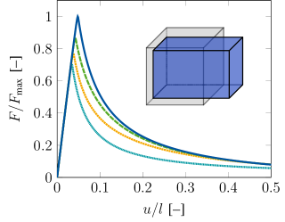
(a) Uniaxial tension

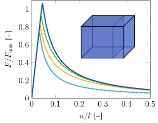
(b) Uniaxial strain

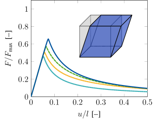
(c) Simple shear

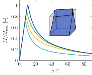
(d) Torsion

Figure 1: Single element studies for uniaxial tension, uniaxial strain, simple shear and torsion. The force-displacement curves are normalized with respect to the maximum force for uniaxial tension for $k_{\mathrm{ani}}=1.00$ with $F_{\text{max}}=8.1251\times 10^{2}~{}[$\mathrm{N}\text{/}$]$. The moment-twist curves are normalized with respect to the maximum moment for $k_{\mathrm{ani}}=1.00$ with $M_{\text{max}}=-2.1427\times 10^{2}~{}[$\mathrm{N}\text{\,}\mathrm{mm}\text{/}$]$.

Uniaxial tension is applied in Fig. 1(a) for different values of the damage anisotropy parameter with $k_{\mathrm{ani}}\in(0.00~{}[$\mathrm{-}$],0.33~{}[$\mathrm{-}$],0.67~{}[$\mathrm{-}$],1.00~{}[$\mathrm{-}$])$, where $k_{\mathrm{ani}}=0.00~{}[$\mathrm{-}$]$ models purely isotropic and $k_{\mathrm{ani}}=1.00~{}[$\mathrm{-}$]$ purely anisotropic material degradation. The normalized force-displacement curves show an increasing maximum retention force followed by a steeper force reduction for an increase of the damage anisotropy parameter $k_{\mathrm{ani}}$. A uniaxial strain state is applied in Fig. 1(b), where the curves show a qualitatively similar behavior to Fig. 1(a). However quantitatively, the maximum retention force for $k_{\mathrm{ani}}=1.00~{}[$\mathrm{-}$]$ is $5.93~{}[$\mathrm{\char 37\relax}\text{/}$]$ higher compared uniaxial tension due to the constrained lateral contraction. Simple shear is applied in Fig. 1(c) and yields a response qualitatively similar to uniaxial tension and uniaxial strain, but the maximum retention force for $k_{\mathrm{ani}}=1.00~{}[$\mathrm{-}$]$ is $34.27~{}[$\mathrm{\char 37\relax}\text{/}$]$ smaller compared to uniaxial tension. Finally, a torsional load is applied in Fig. 1(d) also for different values of the damage anisotropy parameter and confirms the previous observations of Figs. 1(a)-1(c) that for this model a higher material strength corresponds to higher values of damage anisotropy.

3.2 Asymmetrically notched specimen

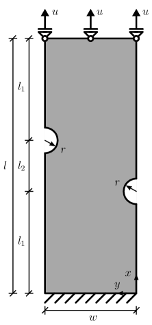
Figure 2: Geometry and boundary value problem for the asymmetrically notched specimen.

The first structural example considers an asymmetrically notched specimen in Fig. 2 under plane strain conditions with the dimensions $l=100~{}[$\mathrm{mm}\text{/}$]$, $l_{1}=40~{}[$\mathrm{mm}\text{/}$]$, $l_{2}=20~{}[$\mathrm{mm}\text{/}$]$, $w=36~{}[$\mathrm{mm}\text{/}$]$, $r=5~{}[$\mathrm{mm}\text{/}$]$ and a thickness of $1~{}[$\mathrm{mm}\text{/}$]$ that was previously studied in e.g. Brepols et al. [2017]. Analogously to van der Velden et al. [2024], this example is investigated using the gradient-extensions of model A, B, and C. The gradient parameter of model A is arbitrarily chosen as $A_{i}^{\text{A}}=1000~{}[$\mathrm{MPa}\text{\,}{\mathrm{mm}}^{2}\text{/}$]$ and the parameters of model B and C are identified as $A_{i}^{\text{B}}=300~{}[$\mathrm{MPa}\text{\,}{\mathrm{mm}}^{2}\text{/}$]$ and $A_{i}^{\text{C}}=3000~{}[$\mathrm{MPa}\text{\,}{\mathrm{mm}}^{2}\text{/}$]$ to obtain the same structural load bearing capacity.

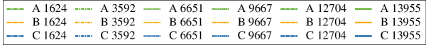
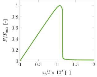
(a) Model A

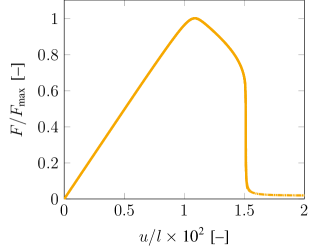
(b) Model B

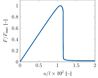
(c) Model C

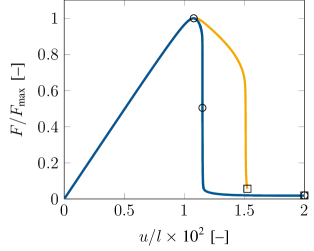
(d) Model comparison (13955 elements)

Figure 3: Force-displacement curves for the mesh convergence study and the model comparison of the asymmetrically notched specimen. The forces are normalized with respect to the maximum force of model C (13955 elements) with $F_{\text{max}}=4.4031\times 10^{4}~{}[$\mathrm{N}\text{/}$]$. In Figs. 3(a), 3(b), and 3(c), the curves obtained with the coarse and fine meshes are essentially congruent. In Fig. 3(d), the squares indicate the snapshots of Fig. 4 and the circles indicate the snapshots of Fig. 5.

The force-displacement curves in Figs. 3(a), 3(b), and 3(c) show the mesh convergence studies for model A, B, and C with the meshes steming from Holthusen et al. [2022a]. All models yield excellent convergence behavior with negligible differences between the results of the coarsest and finest mesh. A model comparison of the structural response with respect to the force-displacement curves is provided in Fig. 3(d) and shows a fine agreement between model A with the full regularization and model C with the reduced volumetric-deviatoric regularization. For model B, the vertical drop in the force-displacement curve is shifted significantly to the right compared to models A and C and, thus, entails a larger amount of dissipated energy in the failure process, which is in line with the results of van der Velden et al. [2024].

(a) Model A

(b) Model B

(c) Model C

Model C

Figure 4: Damage contour plots for the asymmetrically notched specimen with models A, B, and C (13955 elements) at the end of the simulation.

A comparison of the damage contour plots of models A, B, and C for the asymmetrically notched specimen is given in Fig. 4. The crack width and damage affected zone of model B (Fig. 4(b)) are thicker than those of models A and C (Figs. 4(a) and 4(c)) and, thereby, yield a higher energy dissipation. Nevertheless, close agreement between the damage patterns of models A and C is observed.

(a) initial

(b) intermediate

(c) final

Model C

Figure 5: Damage evolution contour plots for the asymmetrically notched specimen with model C (13955 elements).

The evolution of the normal ($D_{xx}$, $D_{yy}$) and shear ($D_{xy}$) components of the damage tensor for model C is presented in Fig. 5, where the position of the snapshots is indicated by the circles in Fig. 3(d). Damage initiates at both notches (Fig. 5(a)), then it forms a damage shear band zone (Fig. 5(b)), in which finally the crack forms (Fig. 5(c)).

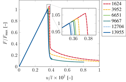
Figure 6: Force-displacement curves for the local damage model for the asymmetrically notched specimen. The forces are normalized with respect to the maximum force of the finest mesh (13955 elements) with $F_{\text{max}}=1.5477\times 10^{4}~{}[$\mathrm{N}\text{/}$]$.

Thereafter, the behavior of the local anisotropic damage without regularization is investigated for the asymmetrically notched specimen. Analogously to Fassin et al. [2019b], the micromorphic parameters are set to $A_{i}=0~{}[$\mathrm{MPa}\text{\,}{\mathrm{mm}}^{2}\text{/}$]$ and $H_{i}=0~{}[$\mathrm{MPa}\text{/}$]$ and, moreover, zero Dirichlet conditions are applied to all nonlocal degrees of freedom, i.e. $\bar{\mathbf{d}}=\bm{0}$. Fig. 6 shows the corresponding force-displacement curves for different finite element mesh discretizations. Using the local formulation, a converged solution is neither achieved with respect to the maximum load bearing capacity of the specimen nor with respect to the amount of dissipated energy.

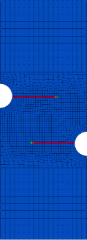
(a) 1624 elements

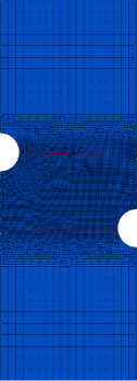
(b) 13955 elements

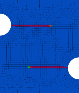
(c) 1624 elements

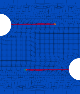
(d) 3592 elements

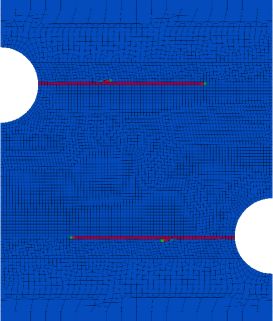
(e) 6651 elements

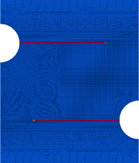
(f) 9667 elements

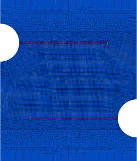
(g) 12704 elements

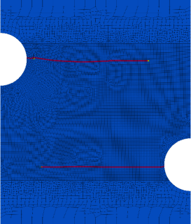
(h) 13955 elements

Figure 7: Damage contour plots with the local damage model for the asymmetrically notched specimen at $u/l\times\text{10}^{\text{2}}=0.4~{}\text{[--]}$. The full specimen is shown with the coarsest and finest mesh in Figs. 7(a) and 7(b) and the center of the specimen is shown for all meshes in Figs. 7(c)-7(h). For this study, the damage variables are averaged over all integration points per element.

Furthermore, the damage contour plots for the study of the local anisotropic damage model are presented in Fig. 7. For all meshes, two cracks form at the notches and propagate horizontally through the specimen, where all cracks localize into a single row of elements. They do not exhibit a tendency of forming a shear crack and to coalesce, which contradicts the results of the gradient-extended solution in Figs. 3-5 and the experimental investigations of e.g. Ambati et al. [2016]. Hence, the utilized artificial viscosity $\eta_{v}=1~{}[$\mathrm{MPa}\text{\,}\mathrm{s}\text{/}$]$ does not yield regularizing effects and the excellent mesh convergence in Figs. 3(a), 3(b), and 3(c) is related to the gradient-extensions of models A, B, and C.

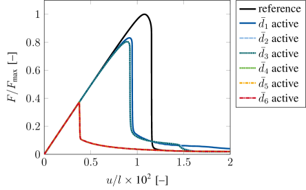
Figure 8: Force-displacement curves for the damage model with regularization of single components of the damage tensor using model A for the asymmetrically notched specimen. The forces are normalized with respect to the maximum force of the reference regularization using the mesh with 1624 elements with $F_{\text{max}}=4.4114\times 10^{4}~{}[$\mathrm{N}\text{/}$]$.

Next, we investigate the possibility of a further reduction of the micromorphic tuple by using only a single degree of freedom. Therefore, model A is again utilized for the simulation of the asymmetrically notched specimen, but each time only a single component of the micromorphic tuple is activated. For example, "$\bar{d}_{1}$ active" refers to the micromorphic gradient parameters $A_{1}^{\text{A}}=1000~{}[$\mathrm{MPa}\text{\,}{\mathrm{mm}}^{2}\text{/}$]$, $A_{2}^{\text{A}}=A_{3}^{\text{A}}=A_{4}^{\text{A}}=A_{5}^{\text{A}}=A_{6}^{\text{A}}=0~{}[$\mathrm{MPa}\text{\,}{\mathrm{mm}}^{2}\text{/}$]$, the micromorphic penalty parameters $H_{1}^{\text{A}}=10^{4}~{}[$\mathrm{MPa}\text{/}$]$, $H_{2}^{\text{A}}=H_{3}^{\text{A}}=H_{4}^{\text{A}}=H_{5}^{\text{A}}=H_{6}^{\text{A}}=0~{}[$\mathrm{MPa}\text{/}$]$, and the Dirichlet boundary conditions $\bar{d}_{2}=\bar{d}_{3}=\bar{d}_{4}=\bar{d}_{5}=\bar{d}_{6}=0~{}[$\mathrm{-}$]$. For model A, $\bar{d}_{1}$ is associated with the regularization of $D_{xx}$, $\bar{d}_{2}$ with $D_{yy}$, $\bar{d}_{3}$ with $D_{zz}$, $\bar{d}_{4}$ with $D_{xy}$, $\bar{d}_{5}$ with $D_{xz}$, and $\bar{d}_{6}$ with $D_{yz}$.

Fig. 8 shows the corresponding force-displacement curves for the regularization of a single component of the damage tensor as well as the reference solution where all six independent components are regularized (from Fig. 3(a)). The regularization of a single component does not suffice for the regularization of the shear crack, since all solutions obtained by a single-component regularization underestimate the maximum force carried by the specimen. The regularization of the normal component $D_{xx}$ by $\bar{d}_{1}$, i.e. the damage tensor component in loading direction, yields an underestimation of $16.86~{}$\mathrm{[}\mathrm{\char 37\relax}\mathrm{]}$$. The regularization of the normal components $D_{yy}$ and $D_{zz}$ by $\bar{d}_{2}$ and $\bar{d}_{3}$ yield an underestimation of $19.77~{}$\mathrm{[}\mathrm{\char 37\relax}\mathrm{]}$$ and $19.55~{}$\mathrm{[}\mathrm{\char 37\relax}\mathrm{]}$$ and the regularization of the shear components $D_{xy}$, $D_{xz}$, and $D_{yz}$ by $\bar{d}_{4}$, $\bar{d}_{5}$, and $\bar{d}_{6}$ each yields an underestimation of $62.80~{}$\mathrm{[}\mathrm{\char 37\relax}\mathrm{]}$$.

(a) $\bar{d}_{1}$ active

(b) $\bar{d}_{2}$ active

(c) $\bar{d}_{3}$ active

(d) $\bar{d}_{4}$ active

(e) reference

Dxx

Figure 9: Damage contour plots for the damage model with regularization of single components of the damage tensor using model A for the asymmetrically notched specimen (1624 elements) at $u/l\times\text{10}^{\text{2}}=0.9~{}\text{[--]}$ in Fig. 8. For this study, the damage variables are averaged over all integration points per element.

(a) $\bar{d}_{1}$ active

(b) $\bar{d}_{2}$ active

(c) $\bar{d}_{3}$ active

(d) $\bar{d}_{4}$ active

(e) reference

Dxx

Figure 10: Damage contour plots for the damage model with regularization of single components of the damage tensor using model A for the asymmetrically notched specimen (1624 elements) at $u/l\times\text{10}^{\text{2}}=2.0~{}\text{[--]}$ in Fig. 8. For this study, the damage variables are averaged over all integration points per element.

The damage contour plots at $u/l\times\text{10}^{\text{2}}=0.9~{}\text{[--]}$ and $u/l\times\text{10}^{\text{2}}=2.0~{}\text{[--]}$ are provided in Figs. 9 and 10. According to the force-displacement curve of the reference solution in Fig. 3(a), an undamaged state exists at $u/l\times\text{10}^{\text{2}}=0.9~{}\text{[--]}$ and the completely damage state at $u/l\times\text{10}^{\text{2}}=2.0~{}\text{[--]}$. The regularization of single damage tensor components influences the specific component’s evolution significantly, but overall fails to obtain the reference solution. If e.g. $\bar{d}_{1}$ is active, it diminishes the damage initiation of $D_{xx}$ whereas $D_{yy}$ already shows signs of localization at the beginning of the failure process (Fig. 9(a)). Upon further loading, $D_{xx}$ still displays a diffuse damage zone at the edges of the crack, but eventually the crack localizes and propagates horizontally instead of slantingly (Fig. 10(a)). The evolution of $D_{yy}$ at further loading yields the same crack pattern, but exhibits a thicker fully damaged zone with little diffusive character at its edges. The activation of $\bar{d}_{2}$ instead of $\bar{d}_{1}$ yields a converse behavior of $D_{xx}$ and $D_{yy}$ (Figs. 9(b) and 10(b)). The activation of $\bar{d}_{3}$ with a regularization of $D_{zz}$ yields a pronounced concentration behavior for $D_{xx}$ and $D_{yy}$ (Figs. 9(c) and 10(c)) analogously to the previously unregularized quantities ($D_{yy}$ in Figs. 9(a) and 10(a) and $D_{xx}$ in Figs. 9(b) and 10(b)). The activation of $\bar{d}_{4}$, $\bar{d}_{5}$, and $\bar{d}_{6}$ with a regularization of $D_{xy}$, $D_{xz}$, and $D_{yz}$ yields a localization of the normal components $D_{xx}$ and $D_{yy}$ into a single row of elements (Figs. 9(d) and 10(d)).

3.3 Rotor blade

After confirming the accuracy of the reduced volumetric-deviatoric regularization of model C in Section 3.2, it is applied for the three-dimensional simulation of a rotor blade specimen. This aims at studying the performance of the universal anisotropic damage framework, here specified for a Neo-Hookean material regularized by model C, to predict damage evolution on a complex structural example. The number of nodes increases significantly in three-dimensional simulations and, thus, only model C is employed for the simulation with two nonlocal degrees of freedom.

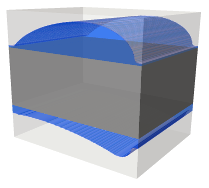
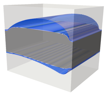
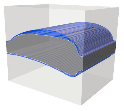
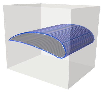
(a) blade production (van der Velden et al. [2023])

(b) rotor

Figure 11: Motivation for the rotor blade specimen. In Fig. 11(a), a single blade is manufactured by electrochemical machining from a solid metal workpiece (dark gray). The tool (light gray) defines the shape and the electrolyte (blue) serves as an electrical conductor for a direct current.

The geometry is inspired by previous works in van der Velden et al. [2023], where the electrochemical machining process is simulated for the manufacturing of a rotor blade (Fig. 11(a)) that can be assembled to an entire rotor (Fig. 11(b)).

Figure 12: Geometry and boundary value problem for the rotor blade specimen. Side view ($x$-$y$) and bottom view ($x$-$z$).

Fig. 12 provides the side and the bottom view of the geometry and boundary value problem where the geometrical dimensions, angles, and positions read $l=20~{}[$\mathrm{mm}\text{/}$]$, $r_{1}=2~{}[$\mathrm{mm}\text{/}$]$, $r_{2}=20~{}[$\mathrm{mm}\text{/}$]$, $r_{3}=25~{}[$\mathrm{mm}\text{/}$]$, $r_{4}=0.5~{}[$\mathrm{mm}\text{/}$]$, $w_{1}=13.5~{}[$\mathrm{mm}\text{/}$]$, $w_{2}=4.882~{}[$\mathrm{mm}\text{/}$]$, $\varphi_{1}=60~{}[$\mathrm{\SIUnitSymbolDegree}\text{/}$]$, $\varphi_{2}=90~{}[$\mathrm{\SIUnitSymbolDegree}\text{/}$]$, $\varphi_{3}=100.137~{}[$\mathrm{\SIUnitSymbolDegree}\text{/}$]$, $\varphi_{4}=117.444~{}[$\mathrm{\SIUnitSymbolDegree}\text{/}$]$, $P_{1}=(-9.0~{}|~{}-15.5884~{}|~{}0.0)~{}[$\mathrm{mm}\text{/}$]$, $P_{2}=(-13.5~{}|~{}-23.3827~{}|~{}0.0)~{}[$\mathrm{mm}\text{/}$]$. The rear edge of the rotor blade is clamped at $z=0~{}[$\mathrm{mm}\text{/}$]$ and the loading case of a pressure load applied from the bottom side is considered.

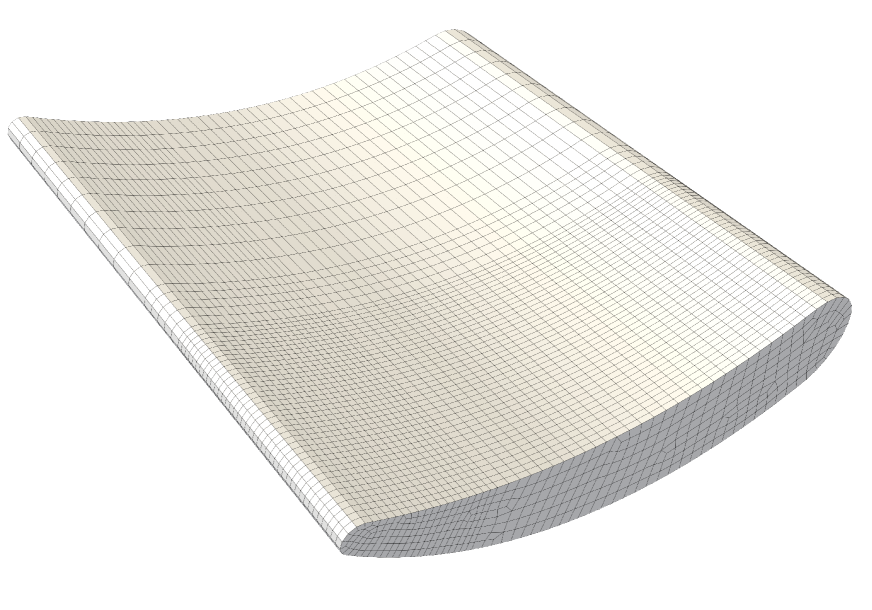
(a) coarsest mesh (21560 elements)

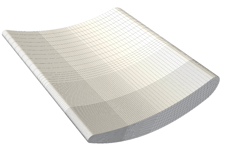
(b) finest mesh (116565 elements)

Figure 13: Finite element meshes for the rotor blade specimen (bottom view).

In Fig. 13, the finite element meshes are shown, which are refined towards the clamped edge and towards the side with the smaller radius due to results of preliminary studies that revealed damage initiation in these regions.

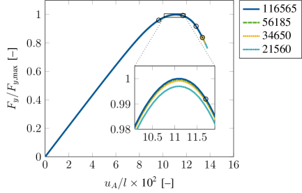
Figure 14: Force-displacement curves for the mesh convergence study of the rotor blade specimen using model C. The forces are normalized with respect to the maximum force of the finest mesh (116565 elements) with $F_{\text{max}}=1.5738\times 10^{4}~{}[$\mathrm{N}\text{/}$]$. The orange boxes indicate the points of comparison for mesh convergence in Figs. 15 and 16. The black circles indicate the points of evaluation for the damage evolution in Figs. 17 and 18.

The normalized force-displacement curves in Fig. 14 depict the sum of the forces in $y$-direction at the clamped edge over the deflection in $y$-direction of point $A$ (see Fig. 12) that is located at position $P_{A}=(-13.5~{}|~{}1.6173~{}|~{}20.0)~{}[$\mathrm{mm}\text{/}$]$. The mesh convergence study yields a close agreement in the force-displacement curves between the results of all meshes. Moreover, the coarsest mesh with 21560 elements underestimates the structural load bearing capacity of the rotor blade that is obtained with the finest mesh with 116565 elements by just $0.30~{}$\mathrm{[}\mathrm{\char 37\relax}\mathrm{]}$$.

(a) 21560 elements

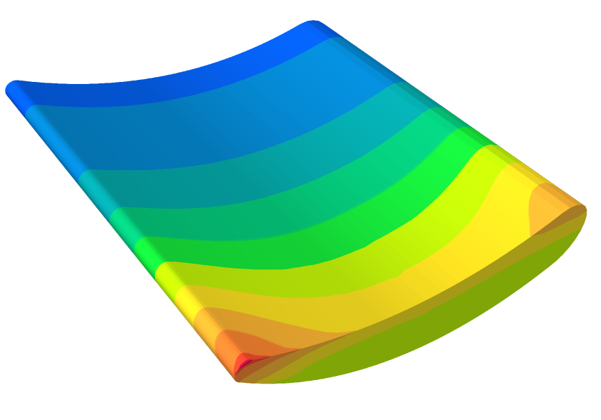
(b) 116565 elements

Figure 15: Contour plots for the mesh convergence of the normal components of the damage tensor for the rotor blade specimen (bottom view).

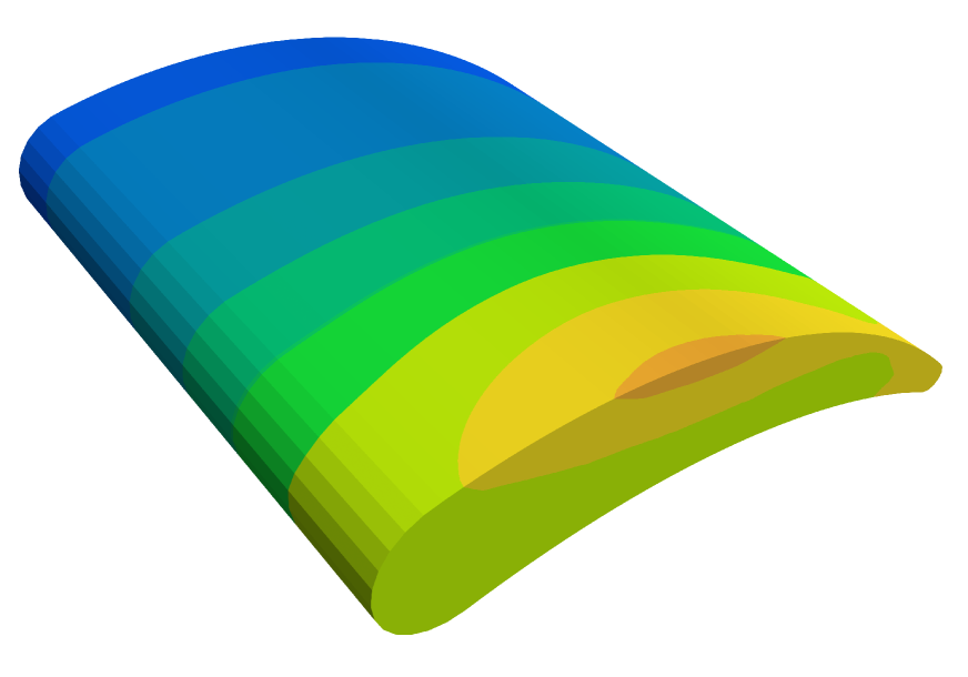
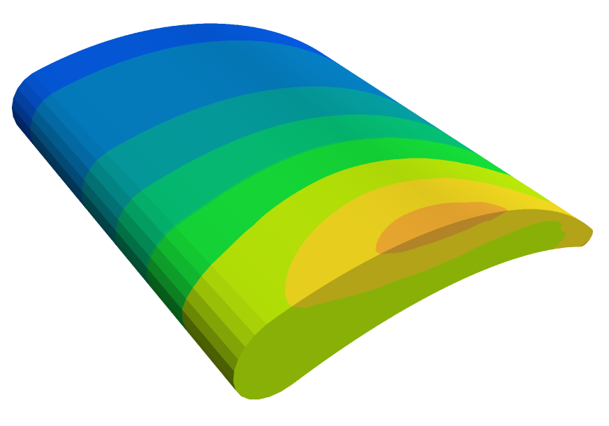
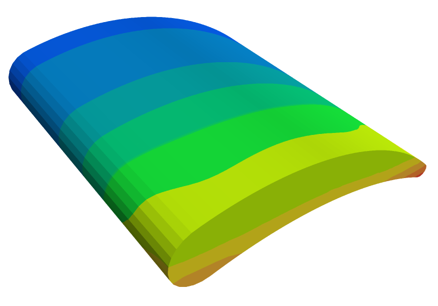
(a) 21560 elements

(b) 116565 elements

Figure 16: Contour plots for the mesh convergence of the normal components of the damage tensor for the rotor blade specimen (top view).

The excellent coarse mesh accuracy, which has been observed with respect to the load bearing capacity, is also reflected in the comparison of the damage contour plots in Figs. 15 (bottom view) and 16 (top view), where high agreement between the normal components of the damage tensor obtained with the coarsest and finest mesh is observed. Fig. 16 reveals the concentrated evolution of the damage tensor components $D_{xx}$ and $D_{yy}$ in the middle of the upper side of the blade at the clamped end. In Fig. 15, the component $D_{zz}$ predominantly evolves at the edges of the lower side at the clamped end. The coarse mesh, in Figs. 15(a) and 16(a), predicts these damage patterns accurately and the fine mesh, in Figs. 15(b) and 16(b), corroborates these results.

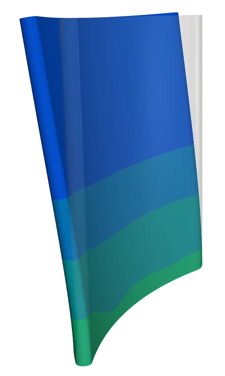
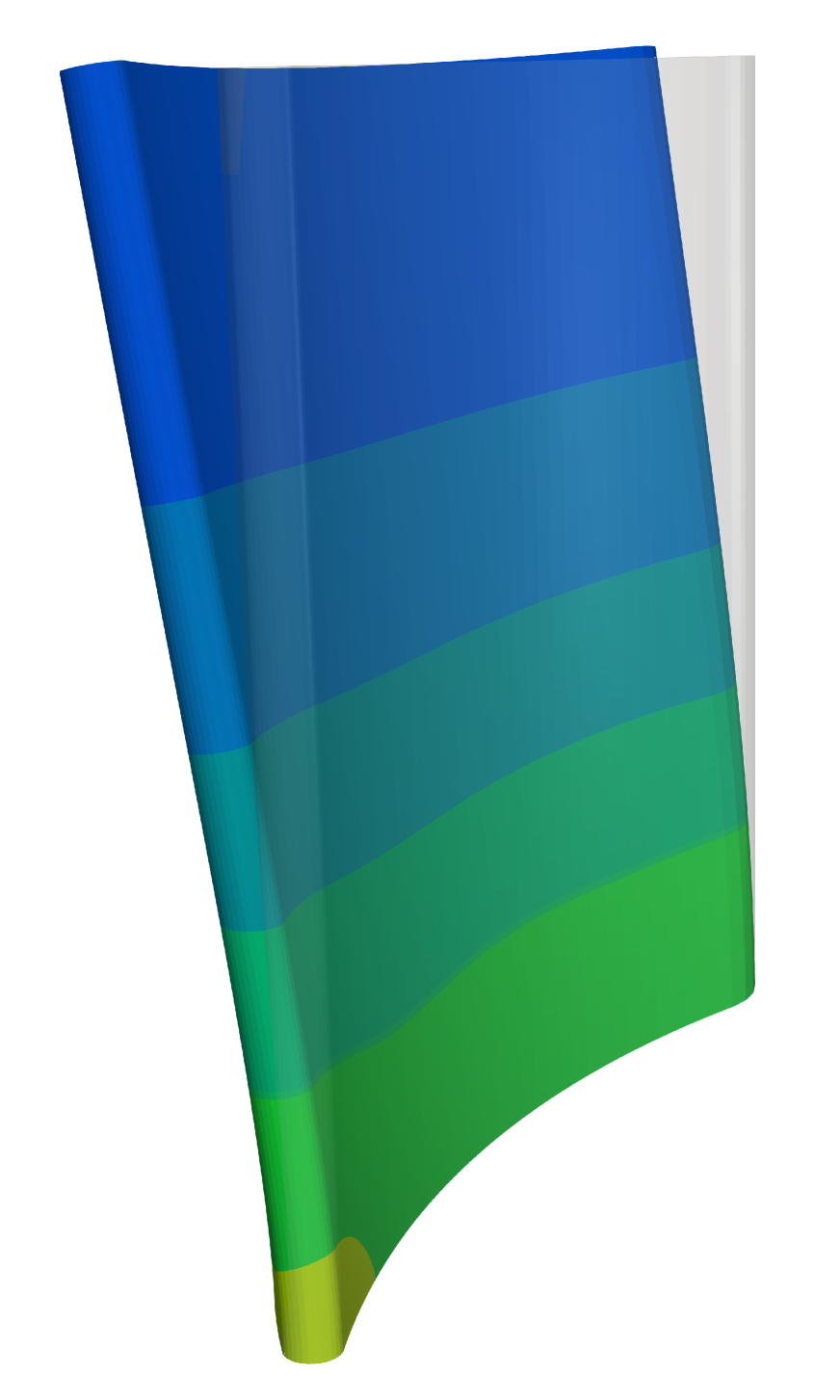
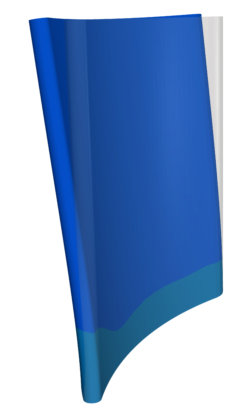
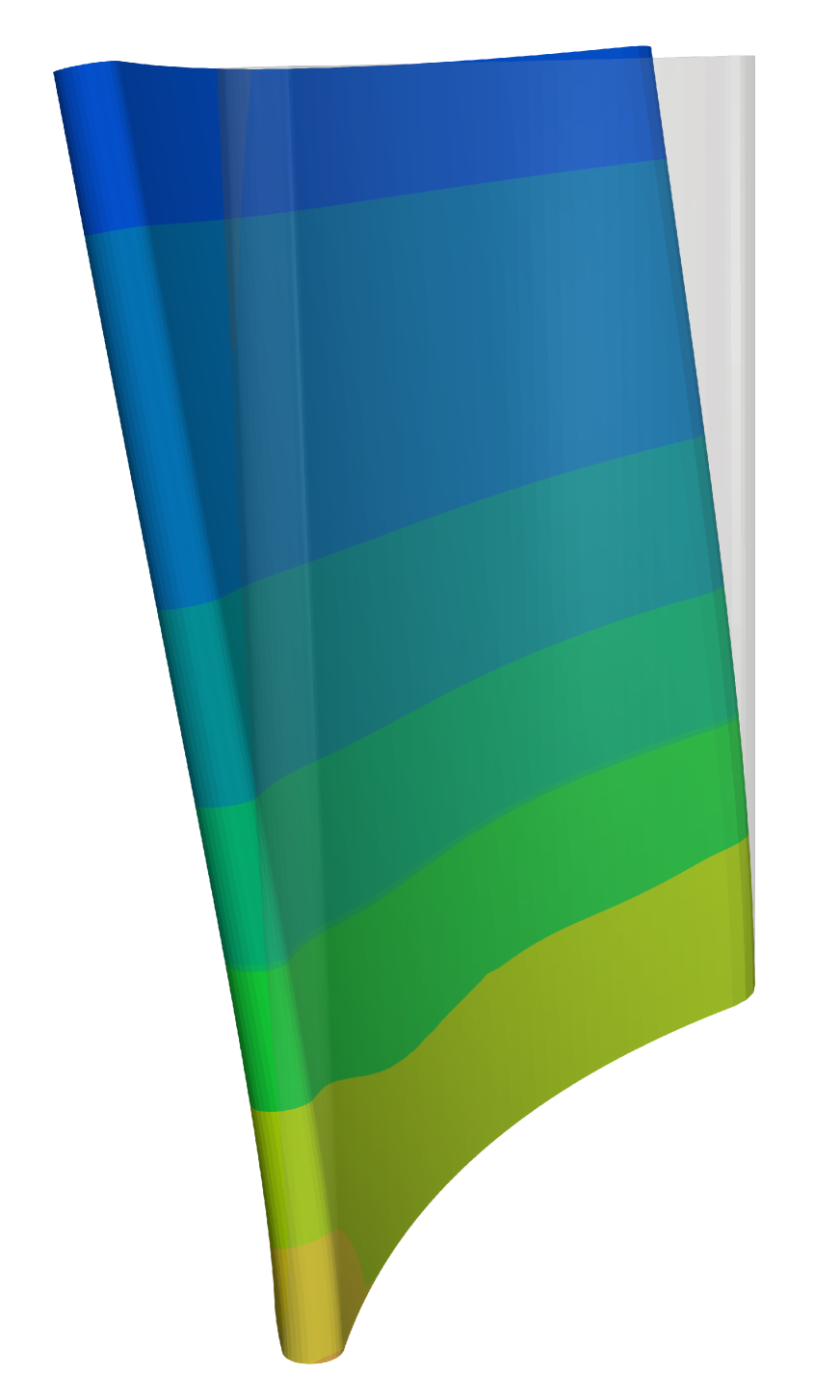
(a) damage initiation

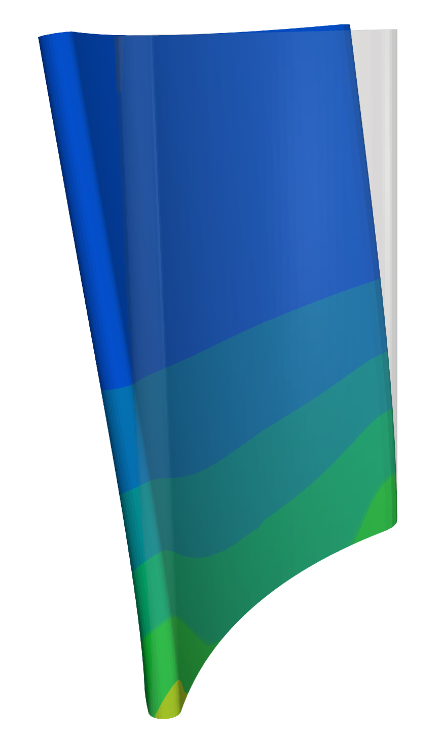
(b) intermediate 1

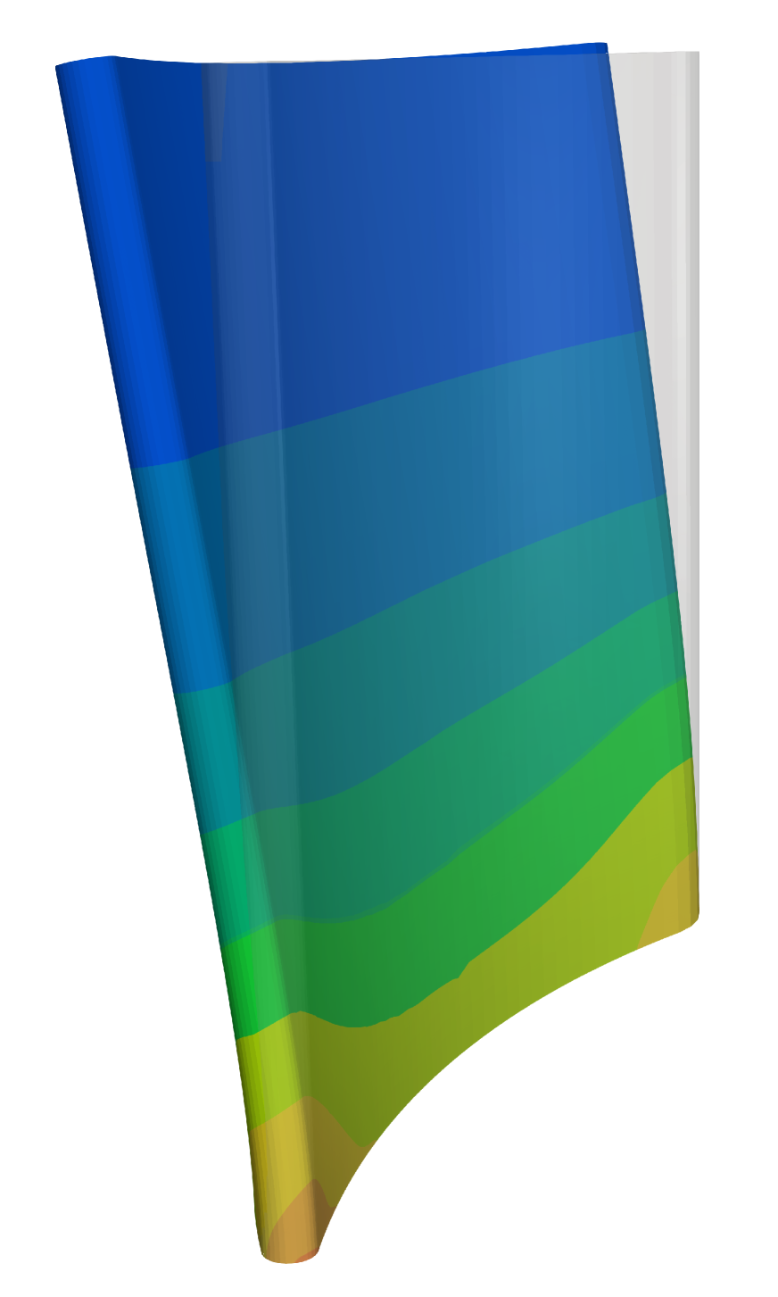
(c) intermediate 2

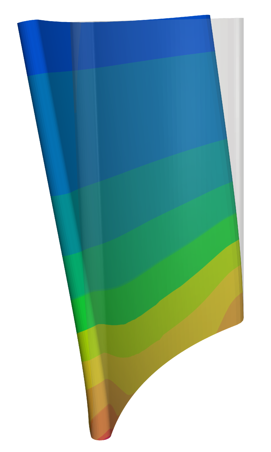
(d) crack opening

dp

Figure 17: Contour plots for the evolution of the normal components of the damage tensor for the rotor blade specimen (side view). The contours are plotted on the deformed configuration and the opaque solid shapes indicate the reference configuration.

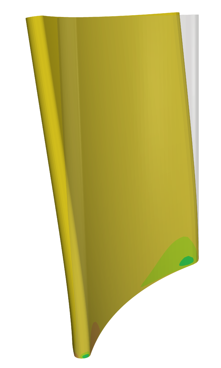
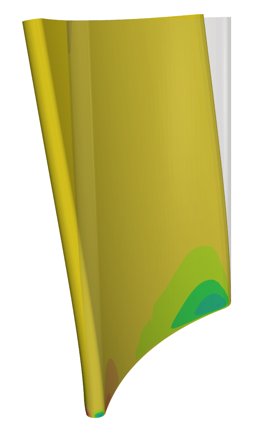
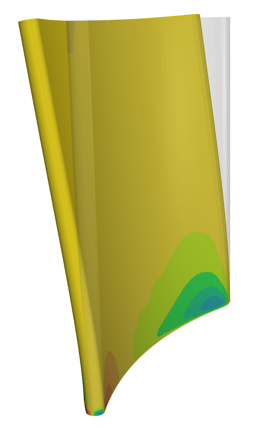
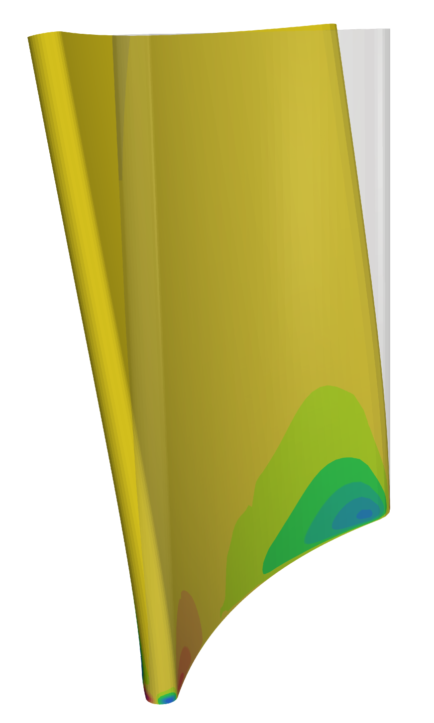
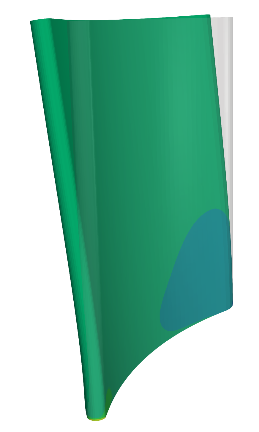
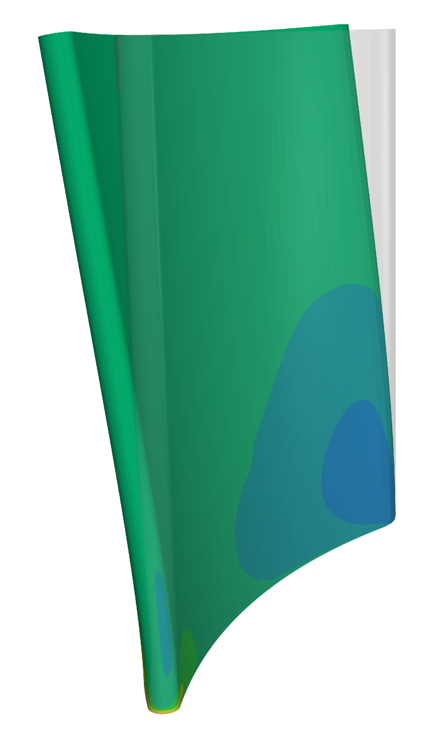
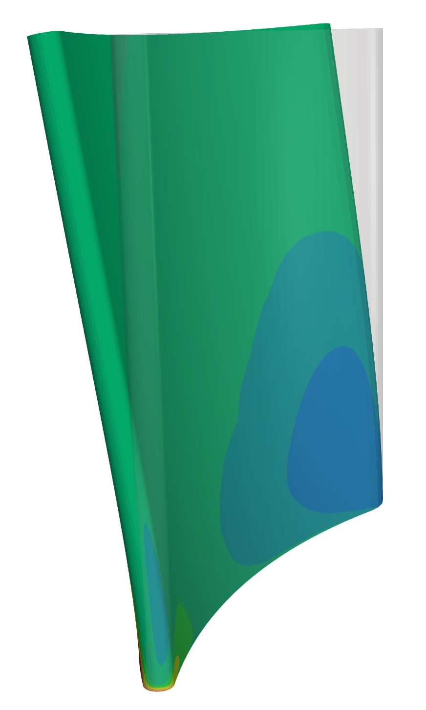
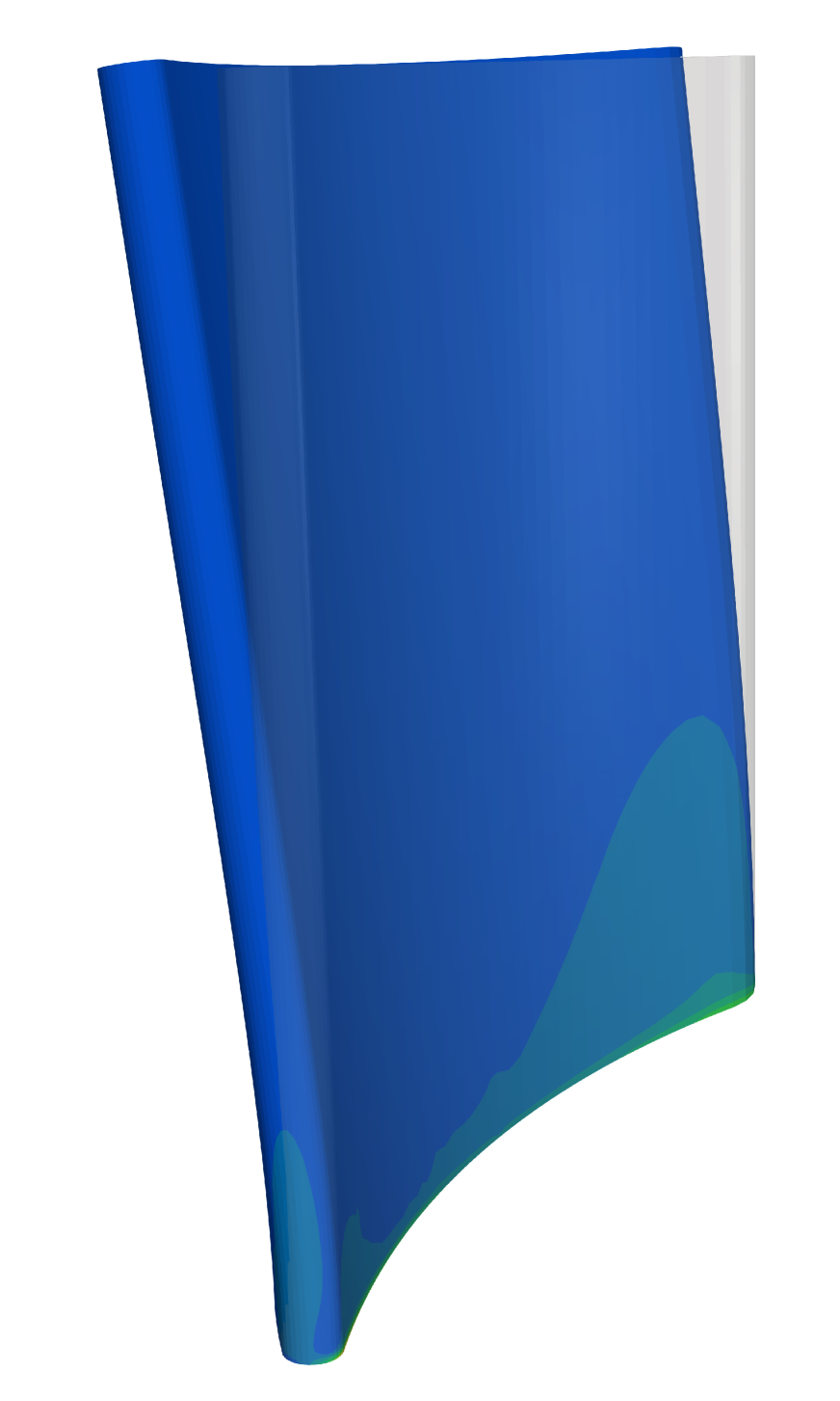
(a) damage initiation

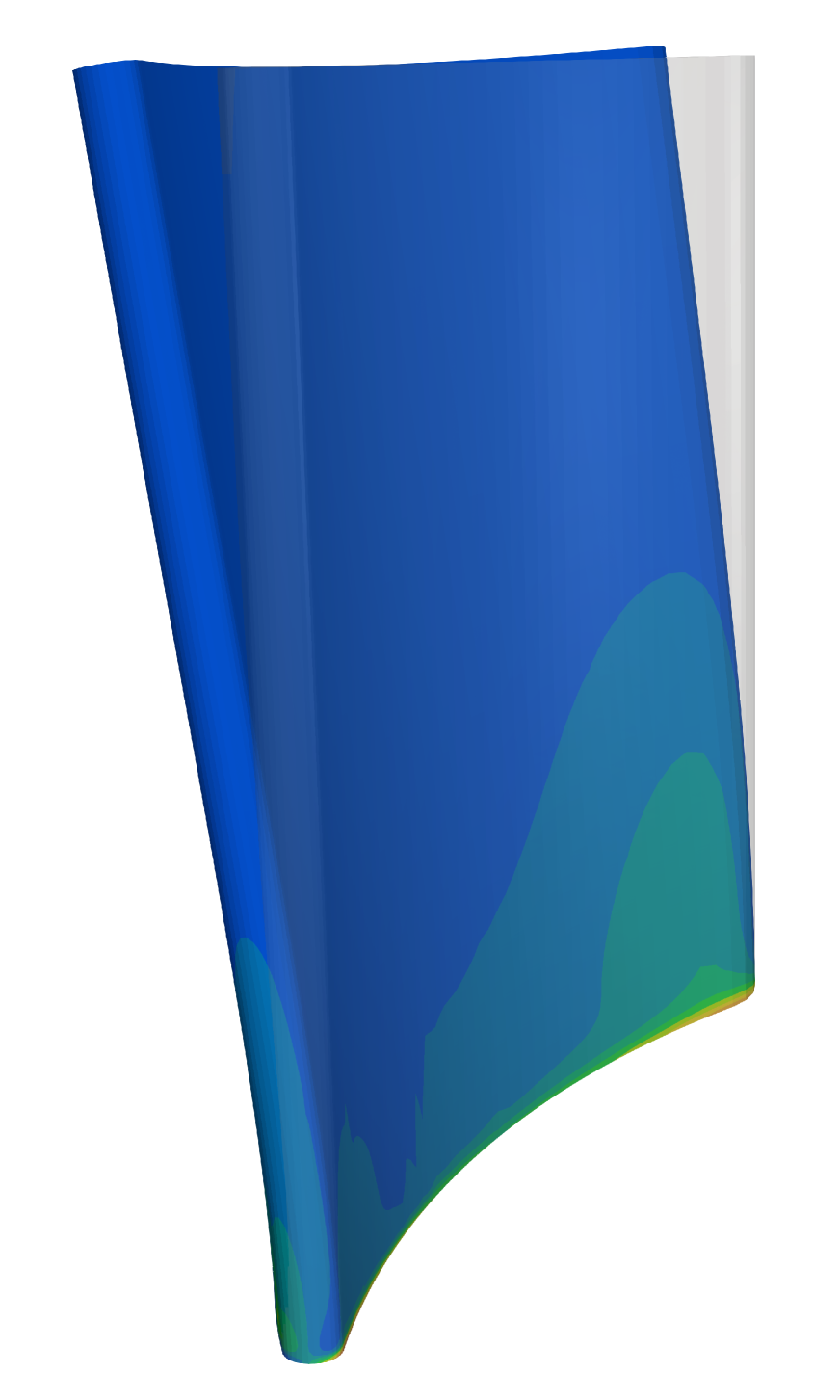
(b) intermediate 1

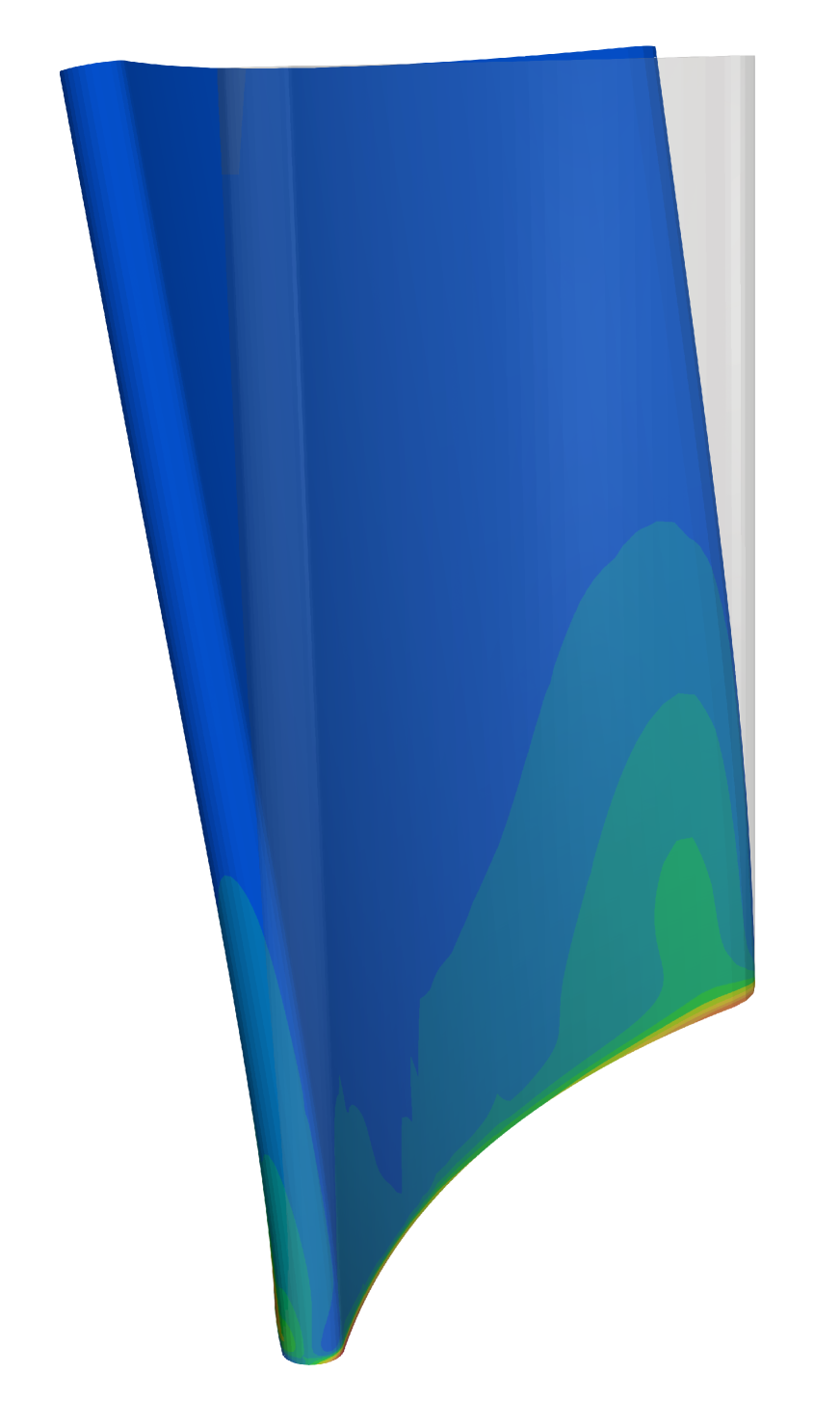
(c) intermediate 2

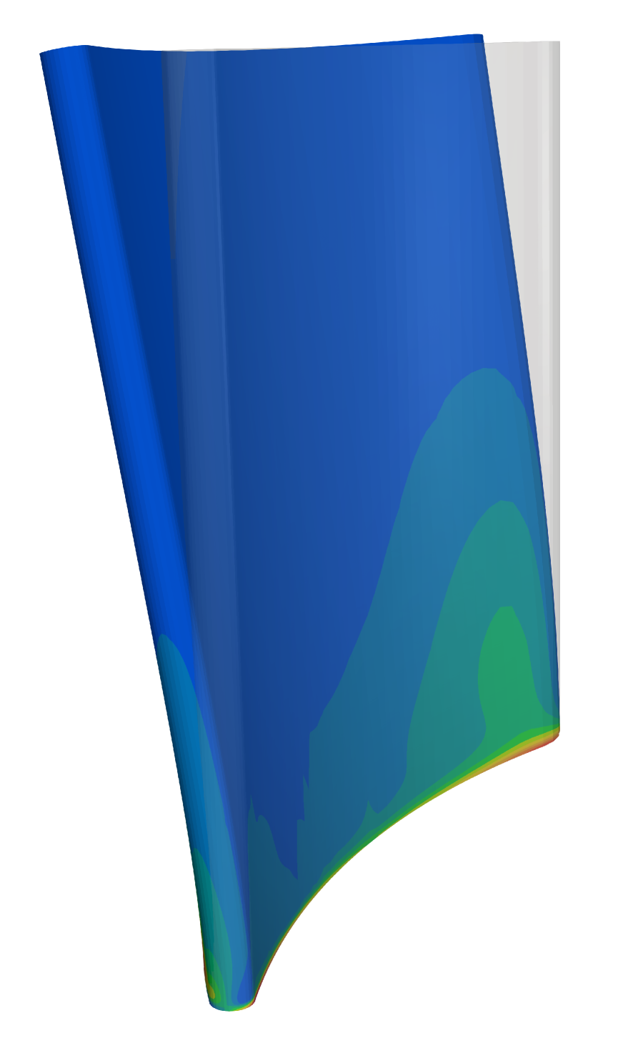
(d) crack opening

dp

Figure 18: Contour plots for the evolution of the shear components of the damage tensor for the rotor blade specimen (side view). The contours are plotted on the deformed configuration and the opaque solid shapes indicate the reference configuration.

The damage evolution process is presented in Figs. 17 and 18 from damage initiation (Figs. 17(a) and 18(a)) to crack opening (Figs. 17(d) and 18(d)) on the deformed configuration. For all normal components, damage initiates at the clamped edge (Fig. 17(a)) and, upon further deformation, progresses with a diffuse damage zone in $z$-direction (Figs. 17(b) and 17(c)). Finally, crack opening occurs by a significant concentration of $D_{zz}$ at the intersection of the free outer edge with radius $r_{4}$ and the clamped edge (Fig. 17(d)). The corresponding evolution of the shear components is presented in Fig. 18 and shows that their peak values occur at the clamped edge.

Summary of the numerical results

The most important findings of the numerical examples with the local formulation, model A (full regularization), model B (reduced principal traces regularization), and model C (reduced volumetric-deviatoric regularization) include:

• The material strength of the local model increases with the degree of damage anisotropy for this specific choice of the Neo-Hookean elastic energy formulation (Fig. 1).

• Models A, B, and C prove excellent coarse mesh accuracy (Figs. 3(a), 3(b), 3(c), and 14).

• Models A and C yield high consistency in the structural force-displacements curves (Fig. 3(d)) and damage contour plots (Figs. 4(a) and 4(c)), while Model B yields a delayed force reduction (Fig. 3(d)) with higher energy dissipation and a thicker damage zone (Fig. 4(b)).

• Utilizing the local anisotropic damage model without gradient-extension results in a false crack path prediction (Fig. 7).

• A single component regularization of the damage tensor proves to be inadequate and yields different degrees of crack localization (Figs. 8, 9, 10).

• With two nonlocal degrees of freedom, model C is an efficient and accurate formulation with extraordinary coarse mesh accuracy (Figs. 14, 15, 16, 17, and 18).

4 Conclusion

In this work, we successfully introduced a universal framework for nonlocal anisotropic damage at finite strains. Due to the design of the degradation functions, arbitrary established hyperelastic finite strain energy formulations can be incorporated into the anisotropic damage model. Furthermore, the generic micromorphic gradient-extension provides a versatile regularization that can prevent any desired number of local quantities from localization.

Initially, the behavior of a specific local anisotropic damage model utilizing a Neo-Hookean energy was investigated in single element studies and yielded an increased material strength for an increase of the degree of damage anisotropy. Thereafter, the model was applied with different gradient-extensions for the simulation of an asymmetrically notched specimen. It confirmed the accurate regularization capabilities of the volumetric-deviatoric regularization steming from previous works for a new local anisotropic damage model. Moreover, the regularization of single components of the damage tensor was studied for the asymmetrically notched specimen and yielded localization regardless of the selection of the gradient-extended quantity. Eventually, the anisotropic damage model with the volumetric-deviatoric regularization was used for the simulation of a rotor blade specimen that was subjected to a pressure load.

Subsequent works could investigate the anisotropic damage behavior of further hyperelastic finite strain energy formulations utilizing the presented framework by straightforwardly replacing the Neo-Hookean energy in the elastic term.

Acknowledgements

Funding granted by the German Research Foundation (DFG) is gratefully acknowledged by T. van der Velden, S. Reese and T. Brepols for project 453715964, by S. Reese and H. Holthusen for project 495926269, by S. Reese, H. Holthusen and T. Brepols for project 417002380 (A01) and by S. Reese and T. Brepols for project 453596084 (B05).

Appendix A Appendix

A.1 General fulfillment of the damage growth criterion

According to the damage growth criterion of Wulfinghoff et al. [2017], the elastic energy has to decrease with any positive semi-definite increment of the damage tensor $\mathrm{d}\bm{D}$ for arbitrary stretch tensors $\bm{\tilde{C}}$. This is mathematically expressed by

$$\psi_{e}(\bm{\tilde{C}},\bm{D}+\mathrm{d}\bm{D})\leq\psi_{e}(\bm{\tilde{C}},\bm{D})\quad\forall\,\bm{\tilde{C}}$$ (44)

or

$$\frac{\partial}{\partial\bm{D}}\,\psi_{e}(\bm{\tilde{C}},\bm{D}):\dot{\bm{D}}\leq 0\quad\forall\,\bm{\tilde{C}}.$$ (45)

Since $\dot{\bm{D}}$ is always positive semi-definite, the partial derivative $\partial\,\psi_{e}(\bm{C},\bm{D})/\partial\bm{D}$ must always satisfy negative semi-definiteness due to the following derivation with $\partial\psi_{e}(\bm{C},\bm{D})/\partial\bm{D}=:\bm{A}$.

Any symmetric second-order tensor $\bm{A}$ is negative semi-definite if

$$\bm{x}\cdot\bm{A}\cdot\bm{x}\leq 0\quad\forall\,\bm{x}\,\backslash\,\{\bm{0}\}$$ (46)

holds. Furthermore, employing the spectral decomposition for the rate of the damage tensor yields

$$\dot{\bm{D}}=\dot{D}_{1}\,\bm{n}_{1}^{\scriptscriptstyle{\color[rgb]{0,0,0}\dot{D}}}\otimes\bm{n}_{1}^{\scriptscriptstyle{\color[rgb]{0,0,0}\dot{D}}}+\dot{D}_{2}\,\bm{n}_{2}^{\scriptscriptstyle{\color[rgb]{0,0,0}\dot{D}}}\otimes\bm{n}_{2}^{\scriptscriptstyle{\color[rgb]{0,0,0}\dot{D}}}+\dot{D}_{3}\,\bm{n}_{3}^{\scriptscriptstyle{\color[rgb]{0,0,0}\dot{D}}}\otimes\bm{n}_{3}^{\scriptscriptstyle{\color[rgb]{0,0,0}\dot{D}}}$$ (47)

where $\dot{D}_{i}\geq 0$ and $\bm{n}_{i}^{\scriptscriptstyle{\color[rgb]{0,0,0}\dot{D}}}$ $(i=1,2,3)$ denote the eigenvalues and eigenvectors of $\dot{\bm{D}}$. Inserting Eq. (47) into Eq. (45) yields

$$\bm{A}:\dot{\bm{D}}=\bm{A}:\left(\dot{D}_{1}\,\bm{n}_{1}^{\scriptscriptstyle{\color[rgb]{0,0,0}\dot{D}}}\otimes\bm{n}_{1}^{\scriptscriptstyle{\color[rgb]{0,0,0}\dot{D}}}+\dot{D}_{2}\,\bm{n}_{2}^{\scriptscriptstyle{\color[rgb]{0,0,0}\dot{D}}}\otimes\bm{n}_{2}^{\scriptscriptstyle{\color[rgb]{0,0,0}\dot{D}}}+\dot{D}_{3}\,\bm{n}_{3}^{\scriptscriptstyle{\color[rgb]{0,0,0}\dot{D}}}\otimes\bm{n}_{3}^{\scriptscriptstyle{\color[rgb]{0,0,0}\dot{D}}}\right).$$ (48)

Using $\bm{A}:(\bm{a}\otimes\bm{b})=\bm{a}\cdot\bm{A}\cdot\bm{b}$, it follows that

$$\bm{A}:\dot{\bm{D}}=\dot{D}_{1}\,\underbrace{\bm{n}_{1}^{\scriptscriptstyle{\color[rgb]{0,0,0}\dot{D}}}\cdot\bm{A}\cdot\bm{n}_{1}^{\scriptscriptstyle{\color[rgb]{0,0,0}\dot{D}}}}_{\leq 0}+\dot{D}_{2}\,\underbrace{\bm{n}_{2}^{\scriptscriptstyle{\color[rgb]{0,0,0}\dot{D}}}\cdot\bm{A}\cdot\bm{n}_{2}^{\scriptscriptstyle{\color[rgb]{0,0,0}\dot{D}}}}_{\leq 0}+\dot{D}_{3}\,\underbrace{\bm{n}_{3}^{\scriptscriptstyle{\color[rgb]{0,0,0}\dot{D}}}\cdot\bm{A}\cdot\bm{n}_{3}^{\scriptscriptstyle{\color[rgb]{0,0,0}\dot{D}}}}_{\leq 0}\leq 0$$ (49)

is generally fulfilled, if $\bm{A}$ is negative semi-definite (cf. Eq. (46)).

Thus, the elastic energy of Eq. (23) must be analyzed with respect to the negative semi-definiteness of $\partial\,\psi_{e}/\partial\bm{D}$. The elastic energy reads with its functional arguments

$$\psi_{e}(\bm{C},\bm{D})=\left(\left(1-k_{\mathrm{ani}}\right)f_{\mathrm{iso}}(\bm{D})+k_{\mathrm{ani}}\,f_{\mathrm{ani}}(\bm{C},\bm{D})\right)\psi_{\star}(\bm{C})$$ (50)

and the partial derivative with respect to the damage tensor

$$\frac{\partial}{\partial\bm{D}}\,\psi_{e}(\bm{C},\bm{D})=\left(\left(1-k_{\mathrm{ani}}\right)\frac{\partial f_{\mathrm{iso}}(\bm{D})}{\partial\bm{D}}+k_{\mathrm{ani}}\,\frac{\partial f_{\mathrm{ani}}(\bm{C},\bm{D})}{\partial\bm{D}}\right)\psi_{\star}(\bm{C}).$$ (51)

Hence, the analysis of the sensitivity of the degradation functions, Eqs. (25) and (26), suffices and yields

$$\frac{\partial f_{\mathrm{iso}}(\bm{D})}{\partial\bm{D}}=\underbrace{{e_{d}}\left(1-\frac{{\rm tr}\left(\bm{D}\right)}{3}\right)^{{e_{d}}-1}}_{\geq 0}\left(-\,\frac{1}{3}\,\bm{I}\right)$$ (52)

and

$$\frac{\partial f_{\mathrm{ani}}(\bm{C},\bm{D})}{\partial\bm{D}}=\underbrace{{f_{d}}\left(1-\frac{{\rm tr}\left(\bm{C}^{2}\bm{D}\right)}{{\rm tr}\left(\bm{C}^{2}\right)}\right)^{{f_{d}}-1}}_{\geq 0}\left(-\frac{\bm{C}^{2}}{{\rm tr}\left(\bm{C}^{2}\right)}\right)$$ (53)

that are both negative semi-definite and, thus, the elastic energy in Eq. (23) generally fulfills the damage growth criterion.

A.2 Isochoric violation of the damage growth criterion

The split of the elastic strain energy into a volumetric and an isochoric part is an established procedure in nonlinear solid mechanics (see e.g. Holzapfel [2000]). In damage modeling, isotropic material degradation can be associated with volumetric deformations and anisotropic material degradation with isochoric deformations. This results in the following composition for the elastic strain energy

$$\psi_{e}=f_{\mathrm{dam}}(\bm{D})\,\psi_{\mathrm{volumetric}}(J)+\psi_{\mathrm{isochoric}}(\bar{\bm{C}},\bm{D})$$ (54)

where $f_{\mathrm{dam}}$ denotes an isotropic degradation function analogously to Eq. (25), $\psi_{\mathrm{volumetric}}$ the volumetric energy contribution, $\psi_{\mathrm{isochoric}}$ the isochoric energy contribution, $J$ the determinant of the deformation gradient $\bm{F}$, and $\bar{\bm{C}}$ the isochoric right Cauchy-Green stretch tensor with $\bar{\bm{C}}=\mathrm{det}(\bm{C})^{-1/3}\bm{C}$. Considering the strong form of the damage growth criterion requires the individual summands of Eq. (54) to fulfill negative semi-definiteness in their partial derivatives with respect to the damage tensor separately. For the volumetric part, this proof is straightforward analogously to Eq. (52).

However, for the isochoric part, the analysis of a given energy will yield the violation of the damage growth criterion. An isochoric energy may read

$$\psi_{\mathrm{isochoric}}(\bar{\bm{C}},\bm{D})=\frac{\mu}{2}\,\mathrm{tr}\left((\bar{\bm{C}}-\bm{I})(\bm{I}-\bm{D})\right)$$ (55)

with

$$\frac{\partial}{\partial\bm{D}}\,\psi_{\mathrm{isochoric}}(\bar{\bm{C}},\bm{D})=-\frac{\mu}{2}\left(\bar{\bm{C}}-\bm{I}\right)$$ (56)

where Eq. (56) is required to be negative semi-definite, i.e. to posses only negative or zero eigenvalues, to fulfill the damage growth criterion. The eigenvalues are analyzed with the spectral form of Eq. (56)

$$-\frac{\mu}{2}\left(\bar{\bm{C}}-\bm{I}\right)=-\frac{\mu}{2}\,\sum_{i=1}^{3}\left(\bar{\lambda}_{i}^{2}-1\right)\bm{N}_{i}\otimes\bm{N}_{i}$$ (57)

where $\bm{N}_{i}$ denote the principal directions of $\bm{C}$ and $\bar{\bm{C}}$ and $\bar{\lambda}_{i}$ the modified principal stretches (cf. Holzapfel [2000]) with

$$\bar{\lambda}_{i}=\frac{\lambda_{i}}{(\lambda_{1}\lambda_{2}\lambda_{3})^{1/3}},\quad i=1,2,3.$$ (58)

Now, assuming a uniaxial stress state with $\lambda_{1}>1$ and $\lambda_{2}=\lambda_{3}<1$ yields for the eigenvalue associated with $\bm{N}_{2}\otimes\bm{N}_{2}$ a positive value, viz.

$$-\frac{\mu}{2}\left(\bar{\lambda}_{2}^{2}\,-\,1\right) =-\frac{\mu}{2}\left(\left(\frac{\lambda_{2}}{(\lambda_{1}\lambda_{2}\lambda_{3})^{1/3}}\right)^{2}-\,1\right)$$ (59)

$$=-\frac{\mu}{2}\left(\left(\frac{\lambda_{2}^{3}}{\lambda_{1}\lambda_{2}\lambda_{3}}\right)^{2/3}-\,1\right)$$ (60)

$$\stackrel{{\scriptstyle\lambda_{2}=\lambda_{3}}}{{=}}\underbrace{-\frac{\mu}{2}}_{<0}\underbrace{\Bigg{(}\bigg{(}\underbrace{\frac{\lambda_{2}}{\lambda_{1}}}_{<1}\bigg{)}^{2/3}-\,1\Bigg{)}}_{<0}>0$$ (61)

and, thus, violates the damage growth criterion.

A.3 Derivative of anisotropic degradation function

The anisotropic degradation function employed in this work reads with the definition in Eq. (26)

$$f_{\mathrm{ani}}=\left(1-\frac{{\rm tr}\big{(}\bm{C}^{2}\bm{D}\big{)}}{{\rm tr}\big{(}\bm{C}^{2}\big{)}}\right)^{f_{d}}$$

and its partial derivative with respect to the right Cauchy-Green stretch tensor $\bm{C}$ follows as

$$\frac{\partial f_{\mathrm{ani}}}{\partial\bm{C}}={f_{d}}\left(1-\frac{{\rm tr}\big{(}\bm{C}^{2}\bm{D}\big{)}}{{\rm tr}\big{(}\bm{C}^{2}\big{)}}\right)^{{f_{d}}-1}\left(-\left(\bm{D}\bm{C}+\bm{C}\bm{D}\right)\frac{1}{{\rm tr}\left(\bm{C}^{2}\right)}+{\rm tr}\left(\bm{C}^{2}\bm{D}\right)\frac{1}{{\rm tr}\left(\bm{C}^{2}\right)^{2}}\,2\,\bm{C}\right).$$ (62)

Evaluating Eq. (62) in the undamaged state yields

$$\left.\displaystyle\frac{\partial f_{\mathrm{ani}}}{\partial\bm{C}}\right|_{\bm{D}=\bm{0}}={f_{d}}\left(1-\frac{{\rm tr}\big{(}\bm{0}\big{)}}{{\rm tr}\big{(}\bm{C}^{2}\big{)}}\right)^{{f_{d}}-1}\left(-\left(\bm{0}+\bm{0}\right)\frac{1}{{\rm tr}\left(\bm{C}^{2}\right)}+{\rm tr}\left(\bm{0}\right)\frac{1}{{\rm tr}\left(\bm{C}^{2}\right)^{2}}\,2\,\bm{C}\right)=\bm{0}$$ (63)

and in the completely damaged state

$$\left.\displaystyle\frac{\partial f_{\mathrm{ani}}}{\partial\bm{C}}\right|_{\bm{D}=\bm{\bm{I}}}={f_{d}}\left(1-\frac{{\rm tr}\big{(}\bm{C}^{2}\big{)}}{{\rm tr}\big{(}\bm{C}^{2}\big{)}}\right)^{{f_{d}}-1}\left(-2\,\bm{C}\frac{1}{{\rm tr}\left(\bm{C}^{2}\right)}+{\rm tr}\left(\bm{C}^{2}\right)\frac{1}{{\rm tr}\left(\bm{C}^{2}\right)^{2}}\,2\,\bm{C}\right)=\bm{0}$$ (64)

and, therewith, $f_{\mathrm{ani}}$ and its derivative fulfill the requirements of Reese et al. [2021] for the anisotropic degradation function.

References

- [1]
- Ahmed et al. [2021] Ahmed, B., Voyiadjis, G. Z. and Park, T. [2021], ‘A nonlocal damage model for concrete with three length scales’, Computational Mechanics 68, 461–486.
- Ahrens et al. [2005] Ahrens, J., Geveci, B. and Law, C. [2005], ParaView: An end-user tool for large data visualization, in ‘Visualization Handbook’, Elsevier. ISBN 978-0123875822.
- Ambati et al. [2016] Ambati, M., Kruse, R. and De Lorenzis, L. [2016], ‘A phase-field model for ductile fracture at finite strains and its experimental verification’, Computational Mechanics 57, 149–167.
- Barfusz et al. [2021a] Barfusz, O., Brepols, T., van der Velden, T., Frischkorn, J. and Reese, S. [2021a], ‘A single gauss point continuum finite element formulation for gradient-extended damage at large deformations’, Computer Methods in Applied Mechanics and Engineering 373, 113440.
- Barfusz et al. [2021b] Barfusz, O., van der Velden, T., Brepols, T., Holthusen, H. and Reese, S. [2021b], ‘A reduced integration-based solid-shell finite element formulation for gradient-extended damage’, Computer Methods in Applied Mechanics and Engineering 382, 113884.
- Barfusz et al. [2022] Barfusz, O., van der Velden, T., Brepols, T. and Reese, S. [2022], ‘Gradient-extended damage analysis with reduced integration-based solid-shells at large deformations’, Computer Methods in Applied Mechanics and Engineering 389, 114317.
- Basaran [2023] Basaran, C. [2023], Introduction to unified mechanics theory with applications, Springer.
- Besson [2010] Besson, J. [2010], ‘Continuum models of ductile fracture: A review’, International Journal of Damage Mechanics 19(1), 3–52.
- Brepols et al. [2017] Brepols, T., Wulfinghoff, S. and Reese, S. [2017], ‘Gradient-extended two-surface damage-plasticity: Micromorphic formulation and numerical aspects’, International Journal of Plasticity 97, 64 – 106.
- Brepols et al. [2020] Brepols, T., Wulfinghoff, S. and Reese, S. [2020], ‘A gradient-extended two-surface damage-plasticity model for large deformations’, International Journal of Plasticity 129, 102635.
- Dorn and Wulfinghoff [2021] Dorn, C. and Wulfinghoff, S. [2021], ‘A gradient-extended large-strain anisotropic damage model with crack orientation director’, Computer Methods in Applied Mechanics and Engineering 387, 114123.
- Fassin et al. [2019a] Fassin, M., Eggersmann, R., Wulfinghoff, S. and Reese, S. [2019a], ‘Efficient algorithmic incorporation of tension compression asymmetry into an anisotropic damage model’, Computer Methods in Applied Mechanics and Engineering 354, 932–962.
- Fassin et al. [2019b] Fassin, M., Eggersmann, R., Wulfinghoff, S. and Reese, S. [2019b], ‘Gradient-extended anisotropic brittle damage modeling using a second order damage tensor – theory, implementation and numerical examples’, International Journal of Solids and Structures 167, 93–126.
- Ferreira et al. [2022] Ferreira, G. V., Campos, E. R. F. S., Neves, R. S., Desmorat, R. and Malcher, L. [2022], ‘An improved continuous damage model to estimate multiaxial fatigue life under strain control problems’, International Journal of Damage Mechanics 31(6), 815–844.
- Forest [2009] Forest, S. [2009], ‘Micromorphic approach for gradient elasticity, viscoplasticity, and damage’, Journal of Engineering Mechanics 135(3), 117–131.
- Forest [2016] Forest, S. [2016], ‘Nonlinear regularization operators as derived from the micromorphic approach to gradient elasticity, viscoplasticity and damage’, Proceedings of the Royal Society A: Mathematical, Physical and Engineering Sciences 472(2188), 20150755.
- Friedlein et al. [2023] Friedlein, J., Mergheim, J. and Steinmann, P. [2023], ‘Efficient gradient enhancements for plasticity with ductile damage in the logarithmic strain space’, European Journal of Mechanics - A/Solids 99, 104946.
- Holthusen et al. [2020] Holthusen, H., Brepols, T., Reese, S. and Simon, J.-W. [2020], ‘An anisotropic constitutive model for fiber-reinforced materials including gradient-extended damage and plasticity at finite strains’, Theoretical and Applied Fracture Mechanics 108, 102642.
- Holthusen et al. [2022a] Holthusen, H., Brepols, T., Reese, S. and Simon, J.-W. [2022a], ‘A two-surface gradient-extended anisotropic damage model using a second order damage tensor coupled to additive plasticity in the logarithmic strain space’, Journal of the Mechanics and Physics of Solids 163, 104833.
- Holthusen et al. [2022b] Holthusen, H., Brepols, T., Simon, J.-W. and Reese, S. [2022b], A gradient-extended anisotropic damage-plasticity model in the logarithmic strain space, in ‘ECCOMAS Congress 2022-8th European Congress on Computational Methods in Applied Sciences and Engineering’, pp. 1–12.
- Holthusen et al. [2024] Holthusen, H., Lamm, L., Brepols, T., Reese, S. and Kuhl, E. [2024], ‘Theory and implementation of inelastic constitutive artificial neural networks’, Computer Methods in Applied Mechanics and Engineering 428, 117063.
- Holzapfel [2000] Holzapfel, G. A. [2000], Nonlinear Solid Mechanics: A Continuum Approach for Engineering, Wiley.
-
HyperWorks [2022]
HyperWorks [2022], ‘Hypermesh’, Altair
Engineering, Inc. .
https://altairhyperworks.com/product/HyperMesh - Jirásek and Desmorat [2019] Jirásek, M. and Desmorat, R. [2019], ‘Localization analysis of nonlocal models with damage-dependent nonlocal interaction’, International Journal of Solids and Structures 174-175, 1–17.
- Lemaitre and Desmorat [2005] Lemaitre, J. and Desmorat, R. [2005], Engineering damage mechanics: ductile, creep, fatigue and brittle failures, Springer.
- Loiseau et al. [2023] Loiseau, F., Oliver-Leblond, C., Verbeke, T. and Desmorat, R. [2023], ‘Anisotropic damage state modeling based on harmonic decomposition and discrete simulation of fracture’, Engineering Fracture Mechanics 293, 109669.
- Mattiello and Desmorat [2021] Mattiello, A. and Desmorat, R. [2021], ‘Lode angle dependency due to anisotropic damage’, International Journal of Damage Mechanics 30(2), 214–259.
- Murakami [2012] Murakami, S. [2012], Continuum damage mechanics: a continuum mechanics approach to the analysis of damage and fracture, Springer Science & Business Media.
- Petrini et al. [2023] Petrini, A., Esteves, C., Boldrini, J. and Bittencourt, M. [2023], ‘A fourth-order degradation tensor for an anisotropic damage phase-field model’, Forces in Mechanics 12, 100224.
- Reese et al. [2021] Reese, S., Brepols, T., Fassin, M., Poggenpohl, L. and Wulfinghoff, S. [2021], ‘Using structural tensors for inelastic material modeling in the finite strain regime – a novel approach to anisotropic damage’, Journal of the Mechanics and Physics of Solids 146, 104174.
- Satouri et al. [2022] Satouri, S., Chatzigeorgiou, G., Benaarbia, A. and Meraghni, F. [2022], ‘A gradient enhanced constitutive framework for the investigation of ductile damage localization within semicrystalline polymers’, International Journal of Damage Mechanics 31(10), 1639–1675.
- Shojaei and Voyiadjis [2023] Shojaei, A. and Voyiadjis, G. Z. [2023], ‘Statistical continuum damage healing mechanics (scdhm)’, International Journal of Damage Mechanics 32(6), 872–885.
- Sprave and Menzel [2023] Sprave, L. and Menzel, A. [2023], ‘A large strain anisotropic ductile damage model — effective driving forces and gradient-enhancement of damage vs. plasticity’, Computer Methods in Applied Mechanics and Engineering 416, 116284.
-
Taylor and Govindjee [2020]
Taylor, R. L. and Govindjee, S. [2020], ‘FEAP - - a finite element analysis program’, University of California, Berkeley .
http://projects.ce.berkeley.edu/feap/manual_86.pdf - van der Velden et al. [2024] van der Velden, T., Brepols, T., Reese, S. and Holthusen, H. [2024], ‘A comparative study of micromorphic gradient-extensions for anisotropic damage at finite strains’, International Journal for Numerical Methods in Engineering p. e7580.
- van der Velden et al. [2023] van der Velden, T., Ritzert, S., Reese, S. and Waimann, J. [2023], ‘A novel numerical strategy for modeling the moving boundary value problem of electrochemical machining’, International Journal for Numerical Methods in Engineering 124(8), 1856–1882.
- Voyiadjis and Kattan [2009] Voyiadjis, G. Z. and Kattan, P. I. [2009], ‘A comparative study of damage variables in continuum damage mechanics’, International Journal of Damage Mechanics 18(4), 315–340.
- Voyiadjis and Kattan [2017] Voyiadjis, G. Z. and Kattan, P. I. [2017], ‘On the decomposition of the damage variable in continuum damage mechanics’, Acta Mechanica 228, 2499–2517.
- Voyiadjis and Kattan [2024] Voyiadjis, G. Z. and Kattan, P. I. [2024], ‘A new unsymmetrical decomposition of the damage variable’, International Journal of Damage Mechanics p. 10567895241245501.
- Wulfinghoff et al. [2017] Wulfinghoff, S., Fassin, M. and Reese, S. [2017], ‘A damage growth criterion for anisotropic damage models motivated from micromechanics’, International Journal of Solids and Structures 121, 21–32.
- Zhang et al. [2022] Zhang, Y., Xu, Y., Wang, Y. and Poh, L. H. [2022], ‘A simple implementation of localizing gradient damage model in abaqus’, International Journal of Damage Mechanics 31(10), 1562–1591.