Method-of-Moments Inference for GLMs and Doubly Robust Functionals under Proportional Asymptotics

Abstract

In this paper, we consider the estimation of regression coefficients and signal-to-noise (SNR) ratio in high-dimensional Generalized Linear Models (GLMs), and explore their implications in inferring popular estimands such as average treatment effects in high dimensional observational studies. Under the “proportional asymptotic” regime and Gaussian covariates with known (population) covariance $\mathbf{\Sigma}$, we derive Consistent and Asymptotically Normal (CAN) estimators of our targets of inference through a Method-of-Moments type of estimators that bypasses estimation of high dimensional nuisance functions and hyperparameter tuning altogether. Additionally, under non-Gaussian covariates, we demonstrate universality of our results under certain additional assumptions on the regression coefficients and $\mathbf{\Sigma}$. We also demonstrate that knowing $\mathbf{\Sigma}$ is not essential to our proposed methodology when the sample covariance matrix estimator is invertible. Finally, we complement our theoretical results with numerical experiments and comparisons with existing literature.

1 Introduction

Statistical inference in Generalized Linear Models (GLMs) (McCullagh and Nelder, 1989), although a classical statistical topic, has witnessed renewed enthusiasm in the modern big data era owing to both theoretical and computational challenges that arise therein (Janková and van de Geer, 2018; Cai et al., 2023; Sur, 2019; Sur et al., 2019; Candès and Sur, 2020; Zhao et al., 2022). This line of research has in turn found resonance in the challenges encountered in the context of inference in observational studies (Chernozhukov et al., 2018; Athey et al., 2018; Jiang et al., 2022; Yadlowsky, 2022; Celentano and Wainwright, 2023). Specifically, estimation of quantities like the causal effect of an exposure on an outcome or estimation of population quantities under missing data typically relies on understanding nuisance functions such as outcome regression and propensity scores (Robins et al., 1994; Scharfstein et al., 1999). These regression functions are often modeled as suitable GLMs, giving rise to scenarios where one needs to adjust for confounders possibly larger in dimension than the available sample size. There now exists a dedicated and comprehensive methodology to deal with inference in both GLMs or observational studies with high dimensional covariates/confounders focused on ideas based on semiparametric theory (Zhang and Zhang, 2014; Javanmard and Montanari, 2014; Janková and van de Geer, 2018; Athey et al., 2018; Smucler et al., 2019; Bradic et al., 2019a, b; Tan, 2020a, b; Dukes and Vansteelandt, 2021; Wang and Shah, 2024; Liu and Wang, 2023; Su et al., 2023). Indeed, this class of methods, in turn, relies on rates of convergence for consistent estimators of high dimensional GLM parameters (Negahban et al., 2012). Moreover, the existence of such a consistent estimator relies on prior ambient unknown low-dimensional (such as sparsity) assumptions in the respective GLMs (Verzelen, 2012; Collier et al., 2017; Cai and Guo, 2017; Bellec and Zhang, 2022). To complement this framework, recent times have witnessed a parallel focus to deal with cases when the entire GLM parameter vector cannot be estimated consistently, and yet there are potential low dimensional summaries of them that can yield themselves to desirable inferential strategies. As a byproduct, one can possibly provide reliable estimation in observational studies. One specific instance that has become popular is when the GLM parameters grow proportionally to the sample size in dimension and do not satisfy additional low-dimensional assumptions. To reflect the inherent difficulty of this setup in terms of the information-theoretic impossibility of estimating the GLM parameter consistently (Verzelen, 2012; Barbier et al., 2019), recent research has coined it as the “inconsistency regime” (Celentano and Wainwright, 2023), and fundamental ideas have already started to carve the contours of this paradigm. A major theme of research in this regime often pertains to initial progress made under Gaussian covariates with known covariance (Bellec and Zhang, 2023) and subsequent demonstration of a universality principle (Zhao et al., 2022; Dudeja et al., 2023a; Han and Shen, 2023). Indeed, the Gaussian assumption is not necessarily a simplifying assumption in the context of development and analysis of the methods developed in the relevant literature – one requires highly involved probabilistic machinery to produce sharp analyses of the derived estimators. However, it turns out that knowledge of the (variance-)covariance matrix of baseline covariates offers enough structure and a priori information that might allow one to bypass complicated estimators and yet obtain remarkably parallel guarantees for inference in GLMs and observational studies in the proportional asymptotic high-dimensional regime. The main purpose of this paper is to take steps in that direction.

1.1 Summary of Results

We summarize the main results of the paper below:

1. We propose moments-based identification strategies (for the precise meaning of identification, we refer readers to Lemma 1 later in the paper) for statistical functionals with nuisance models parameterized as high-dimensional GLMs with the dimension $p$ proportional to $n$ when the covariance matrix of the covariates are known. This allows the construction of estimators of relevant low-dimensional summaries of high-dimensional GLM parameters such as contrasts and signal-to-noise ratio. Moreover, our methods being reliant on only a few low-dimensional moments of the data are computationally efficient.

2. Our moment-based identification and estimation strategies generalize to parallel inferential techniques for popular objects of interest in observational studies such as average treatment effects and mean estimands under missing data – where the analyses depend on two nuisance functions modeled by high dimensional GLMs. Compared to the literature in this class of problems, we do not require sample-splitting and cross-fitting-based ideas owing to our ability to avoid estimating nuisance functions.

3. Our estimators completely bypass the estimation of high dimensional nuisance parameters and are $\sqrt{n}$-Consistent and Asymptotically Normal (CAN) when the baseline covariates are Gaussian under some additional regularity conditions. We further demonstrate the universality of the proposal beyond Gaussian designs in terms of rates of convergence.

4. We also demonstrate that the assumption of knowing the population covariance matrix $\mathbf{\Sigma}$ of the design can be dropped for our proposal when the sample covariance matrix estimator of $\mathbf{\Sigma}$ is invertible and $p<c\cdot n$ for some constant $c$, under Gaussian designs.

5. We conduct extensive numerical experiments to verify the validity of our proposals in finite sample, as well as comparing them with methods from the emerging recent literature. Readers can access the codes for replicating our numerical results from the accompanied GitHub repository.

1.2 Related Works

Our research draws inspiration from several past and ongoing research that aims to address inference in high-dimensional problems. To present a compact survey and comparison with the most related members of this literature we divide our discussions across three broad themes: inference in GLMs, inference for popular observational studies, and the knowledge of variance-covariance matrix of baseline covariates. In each of these sub-parts, we shall further briefly touch upon both ultra-high dimensional regimes under sparsity and proportional high dimensional regimes without sparsity aspects of the results in literature.

1.2.1 Inference in GLMs

In the last two decades, statistical inference for linear and quadratic forms of high dimensional GLM parameters has attracted significant attention from the statistical research community (Verzelen, 2012; Zhang and Zhang, 2014; Javanmard and Montanari, 2014; Dicker, 2014; Verzelen and Gassiat, 2018; Cai and Guo, 2018; Collier et al., 2017; Guo and Cheng, 2022; Battey and Reid, 2023; Celentano and Montanari, 2024). Two complementary tracks of emphasis have emerged in this regard. In the first line of activities, the strategy of inference often draws inspiration from classical semiparametric theory (Janková and van de Geer, 2018) and requires the consistent estimation of ultra high-dimensional (when the dimension $p$ is much larger than the sample size $n$) GLM parameters – which need to rely on apriori low-dimensional assumptions, such as sparsity, on GLM parameter vectors (Collier et al., 2017; Cai and Guo, 2018; Cai et al., 2023). To explore regimes where the existence of consistent estimators of entire GLM parameter vectors are impossible, a complementary theme of inference in GLMs under proportional asymptotics (when the dimension $p$ is proportional to the sample size $n$) has emerged in the last decade (Sur, 2019; Sur et al., 2019; Candès and Sur, 2020; Zhao et al., 2022). In this regime, the strategy typically involves a careful de-biasing surgery on initial suitable yet inconsistent GLM parameter vectors to yield sophisticated CAN estimators of linear and quadratic forms. Indeed, literature in this second direction is more recent and had initially focused on linear models in terms of (i) characterizing the precise risk behavior of convex regularized procedures – first for Gaussian covariates (see Bayati and Montanari (2011); Stojnic (2013); Thrampoulidis et al. (2018); Miolane and Montanari (2021); Celentano et al. (2023) and references therein) and then beyond Gaussian (Gerbelot et al., 2020, 2022; Li and Sur, 2023; Han and Shen, 2023); and (ii) inference of linear and quadratic forms of the parameter vector – albeit mainly in the regime where the design covariance is known apriori (Bellec and Zhang, 2022; Bellec, 2022; Bellec and Zhang, 2023; Song et al., 2024). Results for GLMs are more complete in terms of estimation of the whole parameter vector using convex regularized methods. Parallel methods in GLMs for inference on linear and quadratic forms are more recent, quite case-specific (e.g. consider binary regression with logistic and/or probit link), do not always cover the whole proportional regime (i.e. all aspects ratio considerations of $p/n$) without further assumptions, and often yield coverage guarantees in an average sense on individual coordinates of the GLM parameter vector instead of individually across coordinates (Bellec, 2022). The work conceptually closest to ours is Sawaya et al. (2023), which also proposed moment-based estimators for conducting statistical inference for GLMs. In particular, under assumptions (1) the link function having certain asymmetry (see Section A.8 of Sawaya et al. (2023) for a precise statement) and (2) the covariates $\mathbf{X}$ having zero mean, Sawaya et al. (2023) use only moments of $Y$ to estimate certain quantities in the State Evolution system to conduct inference, hence obviating the requirement of knowing the population covariance matrix $\mathbf{\Sigma}$ of $\mathbf{X}$ or estimating $\mathbf{\Sigma}$ with sufficiently fast convergence rate. However, their methods preclude important GLMs such as the logistic or probit regression.

1.2.2 Inference in Observational Studies

Quantities like average treatment effects and mean parameters in missing data problems have now emerged as quintessential examples of functionals in observational studies where the challenges of high dimensional baseline covariates require careful methodological consideration. Similar to the literature in GLM, two complementary themes have emerged here as well – one regarding ultra-high-dimensional regimes under sparsity and another regarding proportional asymptotic regimes without sparsity but under known Gaussian covariate designs (Celentano and Wainwright, 2023) or for specific functionals with $p<n$ (Yadlowsky, 2022; Jiang et al., 2022). Since the ultra-high-dimensional regime under sparsity has been heavily studied (Athey et al., 2018; Smucler et al., 2019; Bradic et al., 2019a, b; Tan, 2020a, b; Dukes and Vansteelandt, 2021; Wang and Shah, 2024; Liu and Wang, 2023), the results therein are somewhat complete in terms of necessary and sufficient conditions for CAN estimation. However, without Gaussian covariates or the assumption that $p<n$, neither systematic methods nor CAN guarantees exist for the above examples. Our methods aim to fill this gap in the literature. Finally, we remark that our proposed estimators involve second-order $U$-statistics, thus also drawing connections to the growing literature on using Higher-Order $U$-statistics in semiparametric problems in observational studies (Robins et al., 2008, 2023; van der Laan et al., 2021; Kennedy et al., 2024; Bonvini et al., 2024; Liu et al., 2017; Liu and Li, 2023). Also see Remark 10 of Section 2.2 for a more in-depth discussion.

1.2.3 Known (population) Covariance

Our results heavily rely on the knowledge of the variance-covariance matrix of baseline covariates in the study. This known (population) covariance assumption has also been consistently imposed in the literature on the inference of high-dimensional GLMs under proportional asymptotics (Bellec and Zhang, 2023; Bellec, 2022) and there does not seem to be immediate approaches that are suitable to relax this assumption in this inconsistency regime – beyond assuming external semi-supervised data to allow for operator norm consistent estimation of such large dimensional matrices. Indeed, Verzelen and Gassiat (2018) demonstrate the impossibility of estimating or conducting statistical inference on certain functionals in high dimensional regression with unknown arbitrary variance-covariance matrix of the covariates. This does not preclude the designing of procedures informed by a priori assumptions on the variance-covariance matrix of the covariates – a philosophy that has indeed been successfully espoused in the ultra-high-dimensional sparse GLM-based inferences (Verzelen and Gassiat, 2018). Its parallels in the proportional asymptotic regime without sparsity assumptions are quite sporadic and we are only aware of Li and Sur (2023), and to some extent Takahashi and Kabashima (2018), that address this problem for linear forms of the coefficients under the right-rotationally invariant design. Our main results also assume that $\mathbf{\Sigma}$ is known. However, under Gaussian designs, in Section 2.2, we establish $\sqrt{n}$-consistency of our proposed estimator when $\mathbf{\Sigma}$ is unknown as long as the sample covariance matrix estimator of $\mathbf{\Sigma}$ is invertible, demonstrating that knowing $\mathbf{\Sigma}$ is not essential for our proposal.

Organization

To elaborate on the main thesis of the paper, we divide our discussions into the following subsections. In Section 2 we present our results on inference in GLMs followed by its applications in observational studies collected in Section 3. Subsequently, Section 4 validates the theoretical results via numerical experiments. Our article ends by discussing some open problems in Section 5. All the proof details are deferred to the Appendix.

Notation

We denote $(\mathbf{e}_{j},j=1,\cdots,p)$ as the standard bases of ${\mathbb{R}}^{p}$. Given any positive integers $\ell\leq k$, we denote $[k]\coloneqq\{1,\cdots,k\}$ and $[\ell:k]\coloneqq\{\ell,\ell+1,\cdots,k\}$. ${\mathbb{U}}_{n,m}(\cdot)$ is the $m$-th order $U$-statistic operator: given a function $h:{\mathbb{R}}^{m}\rightarrow{\mathbb{R}}$,

$${\mathbb{U}}_{n,m}[h(O_{1},\cdots,O_{m})]\coloneqq\frac{(n-m)!}{n!}\sum_{1\leq i_{1}\neq\cdots\neq i_{m}\leq n}h(O_{i_{1}},\cdots,O_{i_{m}}),$$

where $O_{i}\in{\mathbb{R}}$, for $i\in[n]$. When $m=1$, ${\mathbb{U}}_{n,1}[h(O)]\equiv n^{-1}\sum_{i=1}^{n}h(O_{i})$ then reduces to the empirical mean operator. Given any two vectors $\mathbf{v},\mathbf{u}$ and any matrix ${\mathbb{A}}$ with matching dimensions, we denote $\langle\mathbf{v},\mathbf{u}\rangle_{{\mathbb{A}}}\coloneqq\mathbf{v}^{\top}{\mathbb{A}}\mathbf{u}$ the inner product between $\mathbf{v}$ and $\mathbf{u}$ with respect to ${\mathbb{A}}$; when ${\mathbb{A}}$ is non-negative semi-definite (n.n.s.d.), given any vector $\mathbf{v}$, this inner product induces a norm $\|\mathbf{v}\|_{{\mathbb{A}}}\equiv\mathbf{v}^{\top}{\mathbb{A}}\mathbf{v}$. When ${\mathbb{A}}=\mathbf{I}$, the identity matrix, $\|\cdot\|_{\mathbf{I}}\equiv\|\cdot\|$ reduces to the standard $\ell_{2}$-norm of a vector. Given a random vector $\mathbf{X}$, $\|\mathbf{X}\|_{\psi_{2}}$ denotes its Orlicz $\psi_{2}$-norm. $\lambda_{\min}({\mathbb{A}})$ and $\lambda_{\max}({\mathbb{A}})$, respectively, denote the minimum and maximum eigenvalues of ${\mathbb{A}}$ when it is symmetric and n.n.s.d..

To avoid clutter, we also introduce the short-hand notation ${\mathbb{E}}^{m}(\cdot)\equiv\{{\mathbb{E}}(\cdot)\}^{m}$. A general theme throughout this paper is to construct a multi-valued map $\Psi=(\Psi_{1},\cdots,\Psi_{k}):{\mathcal{D}}\rightarrow{\mathcal{R}}$ from its domain ${\mathcal{D}}$ to its range ${\mathcal{R}}$ using MoM. Given a subset $I\subset[k]$, we let $\Psi_{I}\coloneqq\{\Psi_{j},j\in I\}$ and $\Psi_{I}^{-1}$ be the inverse map of $\Psi_{I}$ if $\Psi_{I}$ is invertible. Given a $k$-th differentiable function $f$, let $f^{(k)}$ denote its $k$-th derivative. Finally, we denote $\|f\|_{q}$ and $\|f\|_{\infty}$ as, respectively, the $L_{q}({\mathbb{P}})$- and $L_{\infty}$-norms of $f$, for $q\geq 1$.

2 Inference in GLMs

In this section, we illustrate our main idea under the following stylized GLM. Suppose that we observe

$$\begin{split}&(Y_{i},\mathbf{X}_{i})_{i=1}^{n}\stackrel{{\scriptstyle\rm i.i.d.}}{{\sim}}\mathbb{P}_{\bm{\beta}},\text{ with }Y_{i}\in\mathbb{R},\,\mathbf{X}_{i}\sim(\bm{\mu},\mathbf{\Sigma})\end{split} \mathsf{GLM}$$ ()

where $\bm{\mu}\in{\mathbb{R}}^{p}$ is the unknown mean vector and $\mathbf{\Sigma}\in{\mathbb{R}}^{p\times p}$ is the known n.n.s.d. population covariance matrix, and there exists a (possibly) nonlinear known link function $\phi:{\mathbb{R}}\rightarrow{\mathcal{R}}\subseteq{\mathbb{R}}$ such that ${\mathbb{E}}(Y|\mathbf{X}=\mathbf{x})=\phi(\mathbf{x}^{\top}\bm{\beta})$ with $\bm{\beta}=(\beta_{1},\ldots,\beta_{p})^{\top}\in\mathbb{R}^{p}$. The range ${\mathcal{R}}$ of $\phi$ is problem specific – e.g. when $Y$ is binary and $\phi$ is the expit/logistic function, then ${\mathcal{R}}\equiv[0,1]$. In this part, we address the question of $\sqrt{n}$-consistent estimation of $\beta_{j}$ for any $j=1,\ldots,p$, the linear form of $\bm{\beta}$ along the direction of $\bm{\mu}$ and the quadratic form of $\bm{\beta}$ with respect to $\mathbf{\Sigma}$:

$$\lambda_{\beta}\coloneqq\bm{\beta}^{\top}\bm{\mu},\,\,\,\,\gamma_{\beta}^{2}\coloneqq\|\bm{\beta}\|_{\mathbf{\Sigma}}^{2}.$$ (1)

In particular, the quadratic form has been used often in applications related to heritability estimation in genetics, e.g. Guo et al. (2019); Song et al. (2024) and references therein. Moreover, as we will see while studying problems of estimating functionals of interest in observational studies in Section 3 with two nuisance functions parameterized by GLMs, our analysis in this section will provide the fundamental building blocks. Therefore, looking forward to the case of simultaneously dealing with two high-dimensional GLMs, for the regression coefficients $\bm{\alpha}$ from a separate GLM, we shall also adopt the same convention by denoting $\lambda_{\alpha}\coloneqq\bm{\alpha}^{\top}\bm{\mu}$ and $\gamma_{\alpha}^{2}\coloneqq\|\bm{\alpha}\|_{\mathbf{\Sigma}}^{2}$. The bounded conditional fourth moment condition on $Y|\mathbf{X}$ is required when establishing the CAN property of our proposed estimators and is imposed here to simplify the exposition (see Appendix G.1).

To discuss the main results of this section and later parts of the paper, we will work with a set of assumptions that we present and discuss before introducing the main ideas of the proposal. First, throughout the paper, we assume the following constraints on $\bm{\mu}$, $\mathbf{\Sigma}$, and the link functions $\phi$.

Assumption $\mathsf{D}$.

There exist universal constants $M>0$ such that

$$M^{-1}\leq\liminf\lambda_{\min}(\mathbf{\Sigma})\leq\limsup\lambda_{\max}(\mathbf{\Sigma})\leq M\text{ and }\|\bm{\mu}\|\leq M.$$

Assumption $\mathsf{L}$.

The link function $\phi$ is assumed to satisfy the following conditions:

1. $\phi$ is three-times differentiable; the first, second, and third derivatives of the link function, together with the link function itself, are integrable with respect to the law of $\mathbf{X}$ and the integrals are all strictly bounded by some universal constant. There also exists a bounded function $f:{\mathbb{R}}\rightarrow{\mathbb{R}}_{+}$ with $\lim_{|t|\rightarrow\infty}f(t)=0$ such that $|\phi^{(\ell)}(t)|\leq e^{t^{2}f(t)}$ for almost all $t\in{\mathbb{R}}$, for $\ell=1,2,3$.

2. $\phi$ is strictly monotone.

Remark 1.

Assumption $\mathsf{L}$ accommodates many GLMs commonly encountered in practice, including the logistic regression, probit regression, Poisson/Negative-Binomial log-linear regression, and etc. ∎

As stated in the Introduction, our focus is on estimating functionals related to GLMs within the framework of the proportional asymptotic regime. Consequently, we also operate under the following assumption between the dimension $p$ and the sample size $n$.

Assumption $\mathsf{C}$.

There exists $\delta\in(0,\infty)$ such that $\lim_{n\rightarrow\infty}p/n\rightarrow\delta$.

Remark 2.

To shorten the exposition, we always assume Assumptions $\mathsf{D}$, $\mathsf{L}$, and $\mathsf{C}$ without explicitly mentioning them unless stated otherwise. ∎

Additionally, we state the following boundedness assumption on $\bm{\beta}$; the second part is imposed to rule out the degenerate case $\bm{\beta}\equiv\bm{0}$.

Assumption $\mathsf{B}$.

• There exists a universal constants $0<\bar{B}<\infty$ such that $\|\bm{\beta}\|\leq\bar{B}$;

• There exists a universal constants $0<\underline{\hbox{\set@color$B$}}\leq\bar{B}$ such that $\|\bm{\beta}\|\geq\underline{\hbox{\set@color$B$}}$.

Finally, we generally need to impose the first part of the following condition on the conditional second moment $Y|\mathbf{X}$. The second part will be needed when establishing the CAN property of our proposed estimator.

Assumption $\mathsf{V}$.

• We assume that $\|\sigma^{2}\|_{2}$ is bounded, where $\sigma^{2}(\cdot)\coloneqq{\mathbb{E}}(Y^{2}|\mathbf{X}=\cdot)$ is the conditional second moment function of $Y$ given $\mathbf{X}$;

• Let $\sigma^{k}(\mathbf{x})\coloneqq{\mathbb{E}}(Y^{k}|\mathbf{X}=\mathbf{x})$ for $k=2,4$. We assume that $\|\sigma^{k}\|_{2}$ is bounded and $\sigma^{k}(\cdot)$ is a GLM sharing the same regression coefficients $\bm{\beta}$, but with possibly different three-times differentiable link functions belonging to $L_{2}({\mathbb{P}})$.

Remark 3.

Assumption $\mathsf{V}$(2) is mainly made to ease exposition when we establish the CAN property of our proposed estimator (see e.g. Proposition 2 and Theorem 2). But it holds for many popular GLMs encountered in practice. For example, when $Y|\mathbf{X}\sim\mathrm{Ber}(\phi(\bm{\beta}^{\top}\mathbf{X}))$, ${\mathbb{E}}(Y^{2}|\mathbf{X})={\mathbb{E}}(Y^{4}|\mathbf{X})=\phi(\bm{\beta}^{\top}\mathbf{X})$; when $Y|\mathbf{X}\sim\mathrm{Pois}(\phi(\bm{\beta}^{\top}\mathbf{X}))$, ${\mathbb{E}}(Y^{2}|\mathbf{X})=\phi(\bm{\beta}^{\top}\mathbf{X})+\phi^{2}(\bm{\beta}^{\top}\mathbf{X})$ and ${\mathbb{E}}(Y^{4}|\mathbf{X})=\phi^{4}(\bm{\beta}^{\top}\mathbf{X})+6\phi^{3}(\bm{\beta}^{\top}\mathbf{X})+7\phi^{2}(\bm{\beta}^{\top}\mathbf{X})+\phi(\bm{\beta}^{\top}\mathbf{X})$. ∎

Finally, it is worth noting that the symbols for the link function, the regression coefficients and the conditional second moment functions in the above assumptions shall be interpreted as generic notations, as in the sequel we may specialize to problem-specific symbols. For example, later in Section 3, we also use $\eta$ for the link function and $\bm{\alpha}$ for the regression coefficients.

2.1 Results for designs that are known to have zero mean

To gather intuition for our method, it is instructive first to consider the following assumptions.

Assumption $\mathsf{G_{0}}$.

$\mathbf{X}\sim\mathrm{N}_{p}(\bm{0},\mathbf{\Sigma})$ or equivalently $\mathbf{Z}\sim\mathrm{N}_{p}(\bm{0},\mathbf{I})$ and $\bm{\mu}$ is known to equal $\bm{0}$.

Our method then essentially relies on the following result, a direct consequence of Stein’s lemma or Gaussian Integration by Parts.

Lemma 1.

Under Model $\mathsf{GLM}$, Assumptions $\mathsf{G_{0}}$, $\mathsf{B}$(1) and $\mathsf{V}$(1), the following hold:

1. Given any fixed vector $\bm{\upsilon}\in{\mathbb{R}}^{p}$ and fixed matrix ${\mathbb{M}}\in{\mathbb{R}}^{p\times p}$, the following system of moment equations holds:

   $${\mathbb{E}}[Y\mathbf{X}^{\top}]{\mathbb{M}}{\mathbb{E}}[\mathbf{X}Y]=\bm{\beta}^{\top}\mathbf{\Sigma}{\mathbb{M}}\mathbf{\Sigma}\bm{\beta}\cdot{\mathbb{E}}^{2}[\phi^{\prime}(\mathbf{X}^{\top}\bm{\beta})],$$ (2a)

   $${\mathbb{E}}[Y\mathbf{X}^{\top}]\bm{\upsilon}={\mathbb{E}}[\phi^{\prime}(\mathbf{X}^{\top}\bm{\beta})]\cdot\bm{\beta}^{\top}\mathbf{\Sigma}\bm{\upsilon}.$$ (2b)

   Consequently, choosing $\bm{\upsilon}=\mathbf{\Sigma}^{-1}\mathbf{e}_{j}$ and ${\mathbb{M}}=\mathbf{\Sigma}^{-1}$, we have

   $$m_{\mathbf{X}Y,2}\coloneqq{\mathbb{E}}[Y\mathbf{X}^{\top}]\mathbf{\Sigma}^{-1}{\mathbb{E}}[\mathbf{X}Y]={\mathbb{E}}^{2}[\phi^{\prime}(\mathbf{X}^{\top}\bm{\beta})]\cdot\gamma_{\beta}^{2}=\mathrm{f}_{1}^{2}(\gamma_{\beta}^{2})\cdot\gamma_{\beta}^{2},$$ (3a)

   $$m_{\beta_{j}}\coloneqq{\mathbb{E}}[Y\mathbf{X}^{\top}]\mathbf{\Sigma}^{-1}\mathbf{e}_{j}={\mathbb{E}}[\phi^{\prime}(\mathbf{X}^{\top}\bm{\beta})]\cdot\beta_{j}\equiv\mathrm{f}_{1}(\gamma_{\beta}^{2})\cdot\beta_{j},$$ (3b)

   where $\mathrm{f}_{1}(t)\coloneqq{\mathbb{E}}[\phi^{\prime}(Z)]$ with $Z\sim\mathrm{N}(0,t)$ for $t\geq 0$. Denote the map induced by (3a) as $\Psi_{\mathsf{GLM}_{0},\beta}:\gamma_{\beta}^{2}\mapsto m_{\mathbf{X}Y,2}$ and the map induced by (3) as $\Psi_{\mathsf{GLM}_{0}}:(\gamma_{\beta}^{2},\beta_{j})\mapsto(m_{\mathbf{X}Y,2},m_{\beta_{j}})$.

2. Further, $\Psi_{\mathsf{GLM}_{0},\beta}$ is a diffeomorphism with $\nabla(\Psi_{\mathsf{GLM}_{0},\beta}^{-1})$ bounded; and the same holds for $\Psi_{\mathsf{GLM}_{0}}$. Consequently, $\gamma_{\beta}^{2}$ and $\beta_{j}$ are identifiable in the sense that the LHS of (6) uniquely determines the value of $(\gamma_{\beta}^{2},\beta_{j})$.

We now unpack Lemma 1, with its proof deferred to the Appendix. Based on the Gaussian design and Stein’s lemma, the moment equations (2) marry the moments on the LHS with certain nonlinear transformation of $\bm{\beta}$ on the RHS. The most important moment equation here is $\Psi_{\mathsf{GLM}_{0},\beta}$ induced by (3a), that maps the quadratic form $\gamma_{\beta}^{2}$ to the moment $m_{\mathbf{X}Y,2}$. Assumption $\mathsf{L}$ on the link function and Assumption $\mathsf{B}$ on $\gamma_{\beta}^{2}$ together ensures that $\Psi_{\mathsf{GLM}_{0},\beta}$ is a diffeomorphism, so $\gamma_{\beta}^{2}=\Psi_{\mathsf{GLM}_{0},\beta}^{-1}(m_{\mathbf{X}Y,2})$ is identified. It will also be made clear later that $\Psi_{\mathsf{GLM}_{0},\beta}$ being a diffeomorphism entails that $\sqrt{n}$-consistent and CAN estimators of $\gamma_{\beta}^{2}$ can be constructed. After identifying $\gamma_{\beta}^{2}$, by solving (3b), $\beta_{j}=m_{\beta_{j}}/\mathrm{f}_{1}(\gamma_{\beta}^{2})$ is as well identified from the moments.

The conclusions in Lemma 1, together with all the other identification results under Gaussian designs in this paper, do not require Assumption $\mathsf{C}$. However, the above moment equations critically rely on the Gaussianity of $\mathbf{X}$. It is natural to ask if, similar to a growing body of work studying universality for regression models under proportional asymptotics (see e.g. Bayati et al. (2015); Montanari and Saeed (2022); Montanari et al. (2023); Hu and Lu (2022); Dudeja et al. (2023b); Lahiry and Sur (2023) and references therein), one could move beyond Gaussian designs and demonstrate the universality of the above identification result. We provide a positive answer to this question following a relaxed identification criterion and shifting the burden of assumption from $\mathbf{X}$ to $\bm{\beta}$.

Definition 1 ($\sqrt{n}$-identifiability).

We say that a low-dimensional target parameter $\psi\in{\mathbb{R}}^{k}$, where $k$ is strictly bounded, of the underlying statistical model ${\mathbb{P}}$ (e.g. Model $\mathsf{GLM}$) is $\sqrt{n}$-identifiable if there exists a (possibly) nonlinear map $\Psi$ from $\psi$ to certain moments defined by ${\mathbb{P}}$ induced by $\psi$, such that if given two different values of the target parameter, $\psi$ and $\psi^{\prime}$, such that $\|\psi-\psi^{\prime}\|\gtrsim n^{-1/2}$, then $\|\Psi(\psi)-\Psi(\psi^{\prime})\|\gtrsim n^{-1/2}$, for sufficiently large $n$.

Assumption $\mathsf{U_{0}}$.

1. $\mathbf{X}=\mathbf{\Sigma}^{1/2}\mathbf{Z}$, where $\mathbf{Z}=(Z_{1},\cdots,Z_{p})^{\top}$ has independent coordinates with zero mean and unit variance, and there exists a universal constant $M>0$ such that $\|Z_{j}\|_{\psi_{2}}\leq M$ for $j=1,\cdots,p$;

2. $\sqrt{p}\mathbf{\Sigma}^{1/2}\bm{\beta}\overset{{\mathcal{W}}_{8}}{\rightarrow}\mathsf{b}$ where $\mathsf{b}\sim\rho$ for some probability measure $\rho$ supported on ${\mathbb{R}}$ and we assume that $\rho$ has bounded first and second moments.

Remark 4.

When $\mathbf{\Sigma}=\mathbf{I}_{p}$, Assumption $\mathsf{U_{0}}$(2) reduces to $\sqrt{p}\bm{\beta}\overset{{\mathcal{W}}_{8}}{\rightarrow}\mathsf{b}$. For general population covariance matrix $\mathbf{\Sigma}$, under $\sqrt{p}\bm{\beta}\overset{{\mathcal{W}}_{8}}{\rightarrow}\mathsf{b}$, the more general assumption will be met under additional assumptions on $\mathbf{\Sigma}$. ∎

We then have the following parallel result of Lemma 1, without assuming that $\mathbf{X}$ is Gaussian.

Lemma 2.

Under the same assumptions as in Lemma 1, except with Assumption $\mathsf{G_{0}}$ replaced by Assumption $\mathsf{U_{0}}$, the system of moment equations appeared in Lemma 1 holds approximately with approximation error $O(p^{-3/4})=O(n^{-3/4})$ as $p\rightarrow\infty$. Thus $\gamma_{\beta}^{2}$ and $\beta_{j}$ are $\sqrt{n}$-identifiable.

The proof of this lemma can be found in Appendix C. Taken together, the above results motivate the following MoM-based estimator of $\gamma_{\beta}^{2}$ and $\beta_{j}$:

$$\begin{split}&\widehat{\gamma}_{\beta}^{2}\coloneqq\Psi_{\mathsf{GLM}_{0},\beta}^{-1}\left(\widehat{m}_{\mathbf{X}Y,2}\mathbbm{1}(\widehat{m}_{\mathbf{X}Y,2}\in\mathcal{R}_{\mathsf{GLM}_{0},\beta})\right),\quad\widehat{m}_{\mathbf{X}Y,2}\coloneqq{\mathbb{U}}_{n,2}[Y_{1}\mathbf{X}_{1}^{\top}\mathbf{\Sigma}^{-1}\mathbf{X}_{2}Y_{2}],\\ &\widehat{\beta}_{j}\coloneqq\frac{\widehat{m}_{\beta_{j}}}{\mathrm{f}_{1}(\widehat{\gamma}_{\beta}^{2})},\quad\widehat{m}_{\beta_{j}}\coloneqq{\mathbb{U}}_{n,1}[Y\mathbf{X}^{\top}\mathbf{\Sigma}^{-1}\mathbf{e}_{j}],\end{split}$$ (4)

where $\mathcal{R}_{\mathsf{GLM}_{0},\beta}\coloneqq\mathrm{Range}(\Psi_{\mathsf{GLM}_{0},\beta})$.

Since $\Psi_{\mathsf{GLM}_{0},\beta}$ is a diffeomorphism, it is clear from the construction above that to prove $\sqrt{n}$-consistency of $\widehat{\gamma}_{\beta}^{2}$ and $\widehat{\beta}_{j}$ one needs to verify $\max\{\mathsf{var}(\widehat{m}_{\mathbf{X}Y,2}),\mathsf{var}(\widehat{m}_{\beta_{j}})\}=O(1/n)$, which is indeed the case (see Appendix C). We next summarize the above reasoning as the following proposition.

Proposition 1.

Under the Assumptions of Lemma 1 or Lemma 2, the following hold:

$$\sqrt{n}(\widehat{\gamma}_{\beta}^{2}-\gamma_{\beta}^{2})=O_{{\mathbb{P}}}(1),\text{ and for any $j=1,\ldots,p$, }\sqrt{n}(\widehat{\beta}_{j}-\beta_{j})=O_{{\mathbb{P}}}(1).$$

In fact, as $n\rightarrow\infty$, we can consider a more precise result and record that the above MoM-based estimators are CAN under the Gaussian design and some additional regularity conditions.

Proposition 2.

Under Model $\mathsf{GLM}$, Assumptions $\mathsf{G_{0}}$, $\mathsf{B}$ and $\mathsf{V}$, if we further assume that $\|\bm{\beta}\|_{f(\mathbf{\Sigma})}^{2}$ converges to some nontrivial limit for $f(\mathbf{\Sigma})=\mathbf{\Sigma},\mathbf{\Sigma}^{2},\mathbf{\Sigma}^{3}$, we have

$$\sqrt{n}(\widehat{\beta}_{j}-\beta_{j})\overset{\mathcal{L}}{\rightarrow}\mathrm{N}(0,\nu_{j}^{2})$$

for some constant $\nu_{j}^{2}>0$ for $j=1,\cdots,p$ and

$$\sqrt{n}(\widehat{\gamma}_{\beta}^{2}-\gamma_{\beta}^{2})\overset{\mathcal{L}}{\rightarrow}\mathrm{N}(0,\nu^{2})$$

for some constant $\nu^{2}>0$.

Remark 5.

It is worth noting that Assumption $\mathsf{B}$(2) is imposed mainly to ensure that the event $\mathbbm{1}(\widehat{m}_{\mathbf{X}Y,2}\in\mathcal{R}_{\mathsf{GLM}_{0},\beta})$ holds with probability converging to 1 such that the constraint does not affect the asymptotic distribution of the $U$-statistic estimator $\widehat{m}_{\mathbf{X}Y,2}$. We conjecture that it is possible to relax this assumption by a more precise analysis of the asymptotic behavior of $\widehat{m}_{\mathbf{X}Y,2}$ close to the boundary $\|\bm{\beta}\|=0$, which is left for future work. ∎

Remark 6.

The CAN property of the proposed MoM-based estimators relies on two separate results: (1) the CLT of first-order and second-order $U$-statistics, followed from the results in Bhattacharya and Ghosh (1992) (see Appendix G for a complete proof) (2) $\Psi_{\mathsf{GLM}_{0},\beta}$ is a diffeomorphism, and its inverse map, $\Psi_{\mathsf{GLM}_{0},\beta}^{-1}$, has bounded derivative so the Delta Method can be applied. ∎

Remark 7.

In Proposition 2 (and similar results related to the CAN property of our proposed estimator in the sequel), we need some extra assumptions on the convergence of inner products such as $\bm{\beta}^{\top}f(\mathbf{\Sigma})\bm{\beta}$. It is worth mentioning that the assumption imposed in the main text might not be tight. By speculating the derivations in Appendix G, one only needs either $\bm{\beta}^{\top}\mathbf{\Sigma}\bm{\beta}$ or $\bm{\beta}^{\top}\mathbf{\Sigma}^{3}\bm{\beta}$ to converge. But to avoid unnecessary technical complications that are irrelevant to the main theme of the paper, we decide not to pursue further in this direction. Also, one can easily find sufficient conditions to establish the convergence of such quantities. As a simple example, when $\mathbf{\Sigma}=\mathbf{I}_{p}$ and $\bm{\beta}$ satisfies Assumption $\mathsf{U_{0}}$, we immediately have $\bm{\beta}^{\top}f(\mathbf{\Sigma})\bm{\beta}$ to converge.

In addition, we also impose an extra condition on ${\mathbb{E}}(Y^{4}|\mathbf{X})$ via Assumption $\mathsf{V}$. This assumption is to ensure that certain re-scaled fourth moments of the $U$-statistics vanish to zero as $n\rightarrow\infty$, which is required based on the proof strategy that we employ (see Lemma 13 and Proposition 4 in Appendix G).

Finally, we do not explicitly specify the form of the asymptotic variance, the form of which is complicated due to the use of second-order $U$-statistics. Nonetheless, in our previous work (Liu et al., 2024), consistent variance estimators based on tweaking the nonparametric bootstrap have been developed and can be used to estimate the variance, and hence conduct inference; also see Section 5.1 for a brief discussion. ∎

Remark 8.

At this point, readers might wonder why we consider moments such as $m_{\mathbf{X}Y,2}$ that involves $\mathbf{X}$. When $\bm{\mu}\equiv\bm{0}$, $Y\in\{0,1\}$ and $\phi(\cdot)=\mathsf{expit}(\cdot)$, it is obvious that all the moments of $Y$ reduce to ${\mathbb{E}}(Y)\equiv 0.5$. Thus without leveraging information of $\mathbf{X}$, it is generally impossible to identify functionals of $\bm{\beta}$, even with the complete knowledge of the distribution of $\mathbf{X}$. This is why the moment-based estimator in Sawaya et al. (2023), based only on ${\mathbb{E}}(Y)$, cannot be applied to logistic or probit regression. ∎

2.2 Results for Gaussian designs with unknown population covariance

As mentioned in the Introduction, our parameter identification and estimation strategies rely on the knowledge of $\mathbf{\Sigma}$ under the proportional asymptotic regime. In this section, we briefly consider relaxing this assumption under Gaussian designs. To simplify our argument, we: (1) focus on establishing only $\sqrt{n}$-consistency but not CAN of the proposed estimator, (2) assume that $\mathbf{X}$ has mean zero, i.e. $\bm{\mu}\equiv\bm{0}$, and finally (3) assume that $n$ is even and we divide the $n$ samples into two parts $I_{1}\coloneqq[n/2]$ and $I_{2}\coloneqq[(n/2+1):2n]$. We use the second part to estimate $\mathbf{\Sigma}$ by the sample Gram matrix

$$\widetilde{\mathbf{\Sigma}}\coloneqq\frac{1}{n/2}\sum_{j\in I_{2}}\mathbf{X}_{j}\mathbf{X}_{j}^{\top}.$$

We also let $\mathbf{\Omega}\coloneqq\mathbf{\Sigma}^{-1}$ and $\widetilde{\mathbf{\Omega}}\coloneqq\widetilde{\mathbf{\Sigma}}^{-1}$ and each element of $\mathbf{\Omega}$ and $\widetilde{\mathbf{\Omega}}$ as, respectively, $\omega_{i,j}$ and $\widetilde{\omega}_{i,j}$ for $i,j\in[p]$.

Remark 9.

The above simplifications are not essential except (3). We conjecture that it is possible to attain $\sqrt{n}$-consistency without using sample splitting to estimate $\mathbf{\Sigma}$ (Liu and Li, 2023), but we decide to report the corresponding results in a separate work. ∎

When $\mathbf{\Sigma}$ is unknown, we propose to estimate $\gamma_{\beta}^{2}$ as in (4), except that $\widehat{m}_{\mathbf{X}Y,2}$ is replaced by

$$\widehat{m}_{\mathbf{X}Y,2}\coloneqq\frac{\frac{n}{2}-p-1}{\frac{n}{2}}\frac{1}{\frac{n}{2}(\frac{n}{2}-1)}\sum_{i_{1}\neq i_{2}\in I_{1}}Y_{i_{1}}\mathbf{X}_{i_{1}}^{\top}\widetilde{\mathbf{\Sigma}}^{-1}\mathbf{X}_{i_{2}}Y_{i_{2}}.$$ (5)

It is worth mentioning that, only in this Section and Appendix D.2, $\widehat{m}_{\mathbf{X}Y,2}$ takes the above form.

It is easy to see that $\widehat{m}_{\mathbf{X}Y,2}$ is an unbiased estimator of $m_{\mathbf{X}Y,2}$. Moreover, we have the following parallel results to Proposition 1, the proof of which can be found in Appendix D.2.

Proposition 3.

Under Assumptions of Lemma 1, when $p+3<n/2$, the following hold:

$$\sqrt{n}(\widehat{\gamma}_{\beta}^{2}-\gamma_{\beta}^{2})=O_{{\mathbb{P}}}(1),\text{ and for any $j=1,\ldots,p$, }\sqrt{n}(\widehat{\beta}_{j}-\beta_{j})=O_{{\mathbb{P}}}(1).$$

The additional assumption $p+3<n/2$ is a result of computing the covariance between any two elements of a random matrix drawn from the Inverse-Wishart distribution; see Lemma 12 for more details.

Remark 10.

$\widehat{m}_{\mathbf{X}Y,2}$ defined in (5) with the prefactor $(\frac{n}{2}-p-1)/\frac{n}{2}$ removed is nothing but the empirical second-order influence function of the functional ${\mathbb{E}}(Y\mathbf{X}^{\top})\mathbf{\Sigma}^{-1}{\mathbb{E}}(\mathbf{X}Y)$, to our knowledge first developed in Liu et al. (2017) and then in Liu et al. (2024). In Liu et al. (2017), however, they did not make distributional assumptions on $\mathbf{X}$ such as Assumption $\mathsf{G_{0}}$ or even Assumption $\mathsf{G}$, resulting in more complicated higher-order $U$-statistics for correcting the bias due to estimating $\mathbf{\Sigma}$ by $\widetilde{\mathbf{\Sigma}}$. In particular, the order can diverge to infinity as $n\rightarrow\infty$. Gaussian designs significantly simplify the diverging-order $U$-statistic estimator to a rescaled second-order $U$-statistic. An interesting question to further explore is which other types of assumptions on $\mathbf{X}$, e.g. right rotationally invariant designs (Li and Sur, 2023), can also reduce higher-order $U$-statistics to simpler second-order $U$-statistics. ∎

Remark 11.

It is worth noting that, for unknown $\mathbf{\Sigma}$, one can adapt the estimators of Guo and Cheng (2022) under linear models; for details, see Appendix D.1.

Furthermore, when $\mathbf{\Sigma}$ is unknown, without estimating $\mathbf{\Sigma}$, one can still test the null hypothesis $H_{0}:\bm{\beta}=\bm{0}$ by simply estimating the quantity ${\mathbb{E}}(Y\mathbf{X}^{\top}){\mathbb{E}}(\mathbf{X}Y)=\bm{\beta}^{\top}\mathbf{\Sigma}^{2}\bm{\beta}$, which equals zero if and only if $H_{0}$ is true, using a $U$-statistic ${\mathbb{U}}_{n,2}(Y_{1}\mathbf{X}_{1}^{\top}\mathbf{X}_{2}Y_{2})$ without the knowledge of $\mathbf{\Sigma}$. ∎

2.3 Results for designs with unknown and possibly non-zero means

Next, we show that the zero covariate-mean condition is not essential to our moment-based approach, but a larger system of moment equations is required to identify relevant parameters in GLMs. The development closely mirrors that of the previous section when $\bm{\mu}$ is known to equal $\bm{0}$. As before, we first set the stage under Gaussian designs.

Assumption $\mathsf{G}$.

$\mathbf{X}\sim\mathrm{N}_{p}(\bm{\mu},\mathbf{\Sigma})$ or equivalently $\mathbf{Z}\sim\mathrm{N}_{p}(\bm{0},\mathbf{I})$.

For short, we let $\bm{\nu}=(\nu_{1},\cdots,\nu_{p})^{\top}\coloneqq\mathbf{\Sigma}^{-1}\bm{\mu}$. The following lemma then generalizes Lemma 1 to the case of Gaussian designs with unknown mean $\bm{\mu}$.

Lemma 3.

Under Model $\mathsf{GLM}$, Assumptions $\mathsf{G}$, $\mathsf{B}$(1), and $\mathsf{V}$(1):

1. The following system of moment equations holds:

   $$m_{Y}\coloneqq{\mathbb{E}}[Y]=\mathrm{f}_{0}({\color[rgb]{0,0,0}\lambda_{\beta}},{\color[rgb]{0,0,0}\gamma_{\beta}^{2}}),$$ (6a)

   $$m_{\mathbf{X},2}\coloneqq{\mathbb{E}}[\mathbf{X}^{\top}]\mathbf{\Sigma}^{-1}{\mathbb{E}}[\mathbf{X}]=\bm{\mu}^{\top}\mathbf{\Sigma}^{-1}\bm{\mu},$$ (6b)

   $$m_{\mathbf{X}Y,\mathbf{X}}\coloneqq{\mathbb{E}}[Y\mathbf{X}^{\top}]\mathbf{\Sigma}^{-1}{\mathbb{E}}[\mathbf{X}]=m_{Y}\cdot m_{\mathbf{X},2}+\mathrm{f}_{1}({\color[rgb]{0,0,0}\lambda_{\beta}},{\color[rgb]{0,0,0}\gamma_{\beta}^{2}})\cdot{\color[rgb]{0,0,0}\lambda_{\beta}},$$ (6c)

   $$m_{\mathbf{X}Y,2}\coloneqq{\mathbb{E}}[Y\mathbf{X}^{\top}]\mathbf{\Sigma}^{-1}{\mathbb{E}}[\mathbf{X}Y]=m_{Y}^{2}\cdot m_{\mathbf{X},2}+\mathrm{f}_{1}^{2}({\color[rgb]{0,0,0}\lambda_{\beta}},{\color[rgb]{0,0,0}\gamma_{\beta}^{2}})\cdot{\color[rgb]{0,0,0}\gamma_{\beta}^{2}}+2\cdot m_{Y}\cdot\mathrm{f}_{1}({\color[rgb]{0,0,0}\lambda_{\beta}},{\color[rgb]{0,0,0}\gamma_{\beta}^{2}})\cdot{\color[rgb]{0,0,0}\lambda_{\beta}},$$ (6d)

   $$m_{\nu_{j}}\coloneqq{\mathbb{E}}[\mathbf{X}]^{\top}\mathbf{\Sigma}^{-1}\mathbf{e}_{j}=\bm{\mu}^{\top}\mathbf{\Sigma}^{-1}\mathbf{e}_{j}=\bm{\nu}^{\top}\mathbf{e}_{j}=\nu_{j},$$ (6e)

   $$m_{\beta_{j}}\coloneqq{\mathbb{E}}[Y\mathbf{X}^{\top}]\mathbf{\Sigma}^{-1}\mathbf{e}_{j}=\mathrm{f}_{0}({\color[rgb]{0,0,0}\lambda_{\beta}},{\color[rgb]{0,0,0}\gamma_{\beta}^{2}})\cdot\nu_{j}+\mathrm{f}_{1}({\color[rgb]{0,0,0}\lambda_{\beta}},{\color[rgb]{0,0,0}\gamma_{\beta}^{2}})\cdot\beta_{j}.$$ (6f)

   where $\mathrm{f}_{k}(s,t)\coloneqq{\mathbb{E}}[\phi^{(k)}(Z)]$ with $Z\sim\mathrm{N}(s,t)$. Denote the forward map induced by this system as

   $$\Psi_{\mathsf{GLM}}=(\Psi_{\mathsf{GLM},1},\Psi_{\mathsf{GLM},2},\cdots\Psi_{\mathsf{GLM},6})^{\top}:(\lambda_{\beta},\gamma_{\beta}^{2})^{\top}\mapsto(m_{Y},m_{\mathbf{X},2},\cdots,m_{\beta_{j}})^{\top}.$$

2. Further, the first four equations of (6), denoted as $\Psi_{\mathsf{GLM},[4]}$, can be reduced to

   $$m_{1}\coloneqq m_{Y}=\mathrm{f}_{0}(\lambda_{\beta},\gamma_{\beta}^{2}),$$ (7a)

   $$m_{2}\coloneqq m_{\mathbf{X}Y,2}+m_{Y}^{2}\cdot m_{\mathbf{X},2}-2\cdot m_{Y}\cdot m_{\mathbf{X}Y,\mathbf{X}}=\mathrm{f}_{1}(\lambda_{\beta},\gamma_{\beta}^{2})\cdot\gamma_{\beta}^{2}.$$ (7b)

   Denote the forward map induced by (7) as $$\Psi_{\mathsf{GLM},\beta}=(\Psi_{\mathsf{GLM},\beta,1},\Psi_{\mathsf{GLM},\beta,2})^{\top}:(\lambda_{\beta},\gamma_{\beta}^{2})^{\top}\mapsto(m_{1},m_{2})^{\top} \Psi_{\mathsf{GLM},\beta} \nabla(\Psi_{\mathsf{GLM},\beta}^{-1}) \lambda_{\beta},\gamma_{\beta}^{2} \beta_{j}$$. Then is a diffeomorphism with bounded. Consequently, , and are identifiable.

The proof of Lemma 3 can be found in Appendix B and Appendix F.1. To establish universality of Lemma 3 beyond Gaussian designs, we need to first generalize Assumption $\mathsf{U_{0}}$ to Assumption $\mathsf{U}$ below.

Assumption $\mathsf{U}$.

1. $\mathbf{X}=\mathbf{\Sigma}^{1/2}\mathbf{Z}+\bm{\mu}$, where $\mathbf{Z}=(Z_{1},\cdots,Z_{p})^{\top}$ has independent coordinates with zero mean, unit variance, and $\max_{j=1}^{p}\|Z_{j}\|_{\psi_{2}}\leq M$ for some universal constant $M>0$;

2. $\sqrt{p}\mathbf{\Sigma}^{1/2}\bm{\beta}\overset{{\mathcal{W}}_{8}}{\rightarrow}\mathsf{b}$ and $\sqrt{p}\mathbf{\Sigma}^{-1/2}\bm{\mu}\overset{{\mathcal{W}}_{8}}{\rightarrow}\mathsf{u}$ where $\mathsf{b}\sim\rho$ and $\mathsf{u}\sim\varrho$ respectively for some probability measures $\rho$ and $\varrho$ supported on ${\mathbb{R}}$ and we assume that both $\rho$ and $\varrho$ have bounded first and second moments.

Lemma 2 can then be generalized as follows, the proof of which can be found in Appendix C.

Lemma 4.

Under the same assumptions as in Lemma 3, except with Assumption $\mathsf{G}$ replaced by Assumption $\mathsf{U}$, the systems of moment equations appeared in Lemma 3 hold approximately with approximation error $O(p^{-3/4})=O(n^{-3/4})$ as $n\rightarrow\infty$.

When the distribution of $\mathbf{X}$ is unknown and one passes to universality after using a Gaussian identification strategy, we conjecture that certain delocalization conditions, such as Assumption $\mathsf{U}$(2) on the (transformed) regression coefficients and covariate mean vector, are necessary. In fact, universality can fail when one starts from a Gaussian identification strategy and Assumption $\mathsf{U}$(2) is violated – as demonstrated via the numerical experiments related to Figures 11 and 12; see Section 4 for more details.

Remark 12.

Compared to the special case of knowing $\bm{\mu}\equiv\bm{0}$ in Section 2.1, it requires extra moment equations (6a) to (6c) to identify $\gamma_{\beta}^{2}$, together with the linear form $\lambda_{\beta}$. When it is known that $\bm{\mu}=\bm{0}$, (6a), (6b), and (6c), respectively, reduce to constants $1/2$, $0$, and $0$. ∎

Remark 13.

When the probability density or mass function $p(\cdot)$ of $\mathbf{X}$ is (partially) known but non-Gaussian, one could leverage the following generalized Stein’s identity (and its higher-order analogues) to obtain similar moment equations

$${\mathbb{E}}[f(\mathbf{X})s(\mathbf{X})]={\mathbb{E}}[f^{\prime}(\mathbf{X})],$$

where $s(\mathbf{X})\coloneqq\nabla p(\mathbf{X})/p(\mathbf{X}):{\mathbb{R}}^{p}\rightarrow{\mathbb{R}}^{p}$ is the score function with respect to the data and $f:{\mathbb{R}}^{p}\rightarrow{\mathbb{R}}$ is any differentiable function such that both sides of the above identity exist. We do not explore these generalizations in this paper and keep it as potential future directions. ∎

Gathering the development thus far, we can construct the following estimator of $(\lambda_{\beta},\gamma_{\beta}^{2})$ based on $\Psi_{\mathsf{GLM},\beta}$ and its inverse map $\Psi_{\mathsf{GLM},\beta}^{-1}$:

$$\begin{split}(\widehat{\lambda}_{\beta},\widehat{\gamma}_{\beta}^{2})\coloneqq\Psi_{\mathsf{GLM},\beta}^{-1}\left(\widehat{m}_{1}\mathbbm{1}\{\widehat{m}_{1}\in{\mathcal{R}}_{\mathsf{GLM},\beta,1}\},\widehat{m}_{2}\mathbbm{1}\{\widehat{m}_{2}\in{\mathcal{R}}_{\mathsf{GLM},\beta,2}\}\right),\end{split}$$ (8)

where

$$\begin{split}\widehat{m}_{1}\coloneqq\widehat{m}_{Y}&\coloneqq{\mathbb{U}}_{n,1}[Y],\quad\widehat{m}_{2}\coloneqq\widehat{m}_{\mathbf{X}Y,2}+\widehat{m}_{Y}^{2}\cdot\widehat{m}_{\mathbf{X},2}-2\cdot\widehat{m}_{Y}\cdot\widehat{m}_{\mathbf{X}Y,\mathbf{X}},\\ \text{and }\widehat{m}_{\mathbf{X},2}\coloneqq{\mathbb{U}}_{n,2}[\mathbf{X}_{1}^{\top}\mathbf{\Sigma}^{-1}\mathbf{X}_{2}],&\,\widehat{m}_{\mathbf{X}Y,\mathbf{X}}\coloneqq{\mathbb{U}}_{n,2}[Y_{1}\mathbf{X}_{1}^{\top}\mathbf{\Sigma}^{-1}\mathbf{X}_{2}],\,\widehat{m}_{\mathbf{X}Y,2}\coloneqq{\mathbb{U}}_{n,2}[Y_{1}\mathbf{X}_{1}^{\top}\mathbf{\Sigma}^{-1}\mathbf{X}_{2}Y_{2}].\end{split}$$ (9)

With $(\widehat{\lambda}_{\beta},\widehat{\gamma}_{\beta}^{2})$, one can estimate $\beta_{j}$ by simply solving (6e) to (6f):

$$\widehat{\beta}_{j}\coloneqq\frac{\widehat{m}_{\beta_{j}}-\mathrm{f}_{0}(\widehat{\lambda}_{\beta},\widehat{\gamma}_{\beta}^{2})\cdot\widehat{m}_{\nu_{j}}}{\mathrm{f}_{1}(\widehat{\lambda}_{\beta},\widehat{\gamma}_{\beta}^{2})}$$

where

$$\widehat{m}_{\nu_{j}}\coloneqq{\mathbb{U}}_{n,1}[\mathbf{X}^{\top}]\mathbf{\Sigma}^{-1}\mathbf{e}_{j},\quad\widehat{m}_{\beta_{j}}\coloneqq{\mathbb{U}}_{n,1}[Y\mathbf{X}^{\top}]\mathbf{\Sigma}^{-1}\mathbf{e}_{j}.$$

Theorem 1.

Under the Assumptions of Lemma 3 or Lemma 4, the following hold:

$$\sqrt{n}\left(\widehat{\lambda}_{\beta}-\lambda_{\beta}\right)=O_{{\mathbb{P}}}(1),\sqrt{n}\left(\widehat{\gamma}_{\beta}^{2}-\gamma_{\beta}^{2}\right)=O_{{\mathbb{P}}}(1),\text{ and for any $j=1,\cdots,p$},\sqrt{n}(\widehat{\beta}_{j}-\beta_{j})=O_{{\mathbb{P}}}(1).$$

The final result in this section generalizes Proposition 2 for the CAN property of our proposed estimators to the case where $\bm{\mu}$ is unknown and possibly non-zero.

Theorem 2.

Under Model $\mathsf{GLM}$, Assumptions $\mathsf{G}$, $\mathsf{B}$ and $\mathsf{V}$, if we further assume that $\langle\mathbf{v}_{1},\mathbf{v}_{2}\rangle_{f(\mathbf{\Sigma})}$ converges to some nontrivial limit for $f(\mathbf{\Sigma})=\mathbf{\Sigma}^{-1},\mathbf{\Sigma},\mathbf{\Sigma}^{2},\mathbf{\Sigma}^{3}$ for $\mathbf{v}_{1},\mathbf{v}_{2}\in\{\bm{\mu},\bm{\beta}\}$, we have

$$\sqrt{n}(\widehat{\beta}_{j}-\beta_{j})\overset{\mathcal{L}}{\rightarrow}\mathrm{N}(0,\nu_{j}^{2})$$

for some constant $\nu_{j}^{2}>0$ for $j=1,\cdots,p$ and

$$\sqrt{n}(\widehat{\gamma}_{\beta}^{2}-\gamma_{\beta}^{2})\overset{\mathcal{L}}{\rightarrow}\mathrm{N}(0,\nu^{2})$$

for some constant $\nu^{2}>0$.

In the proof of the above theorem in Appendix G.2, we unpack the conditions of the theorem further. On a higher level, the convergence of inner products $\langle\mathbf{v}_{1},\mathbf{v}_{2}\rangle_{f(\mathbf{\Sigma})}$ to certain nontrivial limits relates to whether the asymptotic variances of moment estimators based on $U$-statistics, after scaled by $\sqrt{n}$, converge to nontrivial limits. However, we first demonstrate the usefulness of these results for estimating popular parameters such as Doubly Robust Functionals (Robins et al., 2008; Rotnitzky et al., 2021; Chernozhukov et al., 2022) arising in observational studies.

3 Inference in Observational Studies

In this section, we appeal to the discussions in the previous part to develop estimators for some popular quantities arising in the context of observational studies. We only present the case when the covariates under study have a Gaussian distribution with known covariance. The universality of the proposed procedure can be established by analogous arguments in the proof of Lemma 4, and hence omitted to avoid repetition and simplify exposition. The examples we discuss here are popular members of what is now known as the class of Doubly-Robust Functionals (Robins et al., 2008; Rotnitzky et al., 2021; Chernozhukov et al., 2022) where in high dimensional instances of the problem practitioners often aim to model the two high dimensional relevant nuisance parameters of the underlying model through flexible GLMs. Although we consider specific and most popular examples in this class, a potential future research avenue is to extend the results in this section to the entire class of Doubly-Robust Functionals characterized in Rotnitzky et al. (2021).

We divide our discussions into three subsections: estimation of causal effects of binary treatment in linear structural models, estimating quantities under missing data, and estimating generalized covariance measure (or equivalently expected conditional covariance (Liu et al., 2024)) that have gained popularity in recent literature on conditional independence testing (Shah and Peters, 2020; Christgau et al., 2023). Throughout this section, we assume that we have access to $n$ i.i.d. copies of the triples $(\mathbf{X}_{i},A_{i},Y_{i})_{i=1}^{n}\overset{\rm i.i.d.}{\sim}{\mathbb{P}}$ where $\mathbf{X}$ is the covariates or the design matrix, except for Section 3.2 with a minor modification.

3.1 Causal Effect of a Binary Treatment under Linear Structural Causal Models

First, we consider the task of estimating the causal effect of a binary treatment $A\in\{0,1\}$ on an outcome $Y$ in a linear structural model. Our goal is to estimate the parameter $\psi$ in the following data generating model with the outcome regression a linear model and the propensity score a GLM with link $\phi$.

$$Y=\psi\cdot A+\bm{\beta}^{\top}\mathbf{X}+\varepsilon,\quad A|\mathbf{X}\sim\mathrm{Ber}\left(\phi(\bm{\alpha}^{\top}\mathbf{X})\right), \mathsf{CE}$$ ()

where $\varepsilon$ has mean zero and bounded second moment given $\mathbf{X},A$.

For convenience, we let $\bm{\mu}_{1}\coloneqq{\mathbb{E}}(\mathbf{X}A)$, $\lambda_{\alpha,1}\coloneqq\bm{\alpha}^{\top}\bm{\mu}_{1}$ and $\lambda_{\beta,1}\coloneqq\bm{\beta}^{\top}\bm{\mu}_{1}$. The following lemma characterizes the moment equations under Model $\mathsf{CE}$, and the derivation can be found in Appendix F.

Lemma 5.

Under Model $\mathsf{CE}$, Assumptions $\mathsf{G}$, $\mathsf{B}$(1) on both $\bm{\alpha}$ and $\bm{\beta}$, and $\mathsf{V}$(1) on both $A|\mathbf{X}$ and $Y|\mathbf{X},A$, the following system of moment equations holds:

$$m_{A}\coloneqq{\mathbb{E}}(A),$$ (10a)

$$m_{Y}\coloneqq{\mathbb{E}}(Y)=\psi\cdot m_{A}+\lambda_{\beta},$$ (10b)

$$m_{AY}\coloneqq{\mathbb{E}}(AY)=(\psi+\lambda_{\beta})\cdot m_{A}+\gamma_{\alpha,\beta}\cdot\mathrm{f}_{1}(\lambda_{\alpha},\gamma_{\alpha}^{2}),$$ (10c)

$$m_{\mathbf{X},2}\coloneqq{\mathbb{E}}(\mathbf{X})^{\top}\mathbf{\Sigma}^{-1}{\mathbb{E}}(\mathbf{X})=\bm{\mu}^{\top}\mathbf{\Sigma}^{-1}\bm{\mu},$$ (10d)

$$m_{\mathbf{X}A,\mathbf{X}}\coloneqq{\mathbb{E}}(A\mathbf{X})^{\top}\mathbf{\Sigma}^{-1}{\mathbb{E}}(\mathbf{X})=\bm{\mu}_{1}^{\top}\mathbf{\Sigma}^{-1}\bm{\mu},$$ (10e)

$$m_{\mathbf{X}A,2}\coloneqq{\mathbb{E}}(A\mathbf{X}^{\top})\mathbf{\Sigma}^{-1}{\mathbb{E}}(\mathbf{X}A)=m_{A}\cdot m_{\mathbf{X}A,\mathbf{X}}+\mathrm{f}_{1}(\lambda_{\alpha},\gamma_{\alpha}^{2})\cdot\lambda_{\alpha,1},$$ (10f)

$$m_{\mathbf{X}A,\mathbf{X}Y}\coloneqq{\mathbb{E}}(A\mathbf{X}^{\top})\mathbf{\Sigma}^{-1}{\mathbb{E}}(\mathbf{X}Y)=\psi\cdot m_{\mathbf{X}A,2}+\lambda_{\beta,1},$$ (10g)

$$m_{\mathbf{X}AY,\mathbf{X}A}\coloneqq{\mathbb{E}}(YA\mathbf{X}^{\top})\mathbf{\Sigma}^{-1}{\mathbb{E}}(\mathbf{X}A)=\psi\cdot m_{\mathbf{X}A,2}+m_{A}\cdot\lambda_{\beta,1}+\lambda_{\beta}\cdot m_{A}\cdot m_{\mathbf{X}A,\mathbf{X}}$$ (10h)

$$+\mathrm{f}_{1}(\lambda_{\alpha},\gamma_{\alpha}^{2})\cdot\left(\lambda_{\beta}\cdot\lambda_{\alpha,1}+\gamma_{\alpha,\beta}\cdot m_{\mathbf{X},\mathbf{X}A}\right)+\mathrm{f}_{2}(\lambda_{\alpha},\gamma_{\alpha}^{2})\cdot\gamma_{\alpha,\beta}\cdot\lambda_{\alpha,1},$$

where the definition of $\mathrm{f}_{k}$ appears in the statement of Lemma 3.

In addition, denote the forward map induced by the RHS of the above system as

$$\Psi_{\mathsf{CE}}\coloneqq \left(\Psi_{\mathsf{CE},1},\cdots,\Psi_{\mathsf{CE},8}\right):\left(\psi,\lambda_{\alpha},\gamma_{\alpha}^{2},\lambda_{\beta},\gamma_{\alpha,\beta},\lambda_{\alpha,1},\lambda_{\beta,1}\right)$$

$$\mapsto\left(m_{A},m_{Y},m_{AY},m_{\mathbf{X},\mathbf{X}A},m_{\mathbf{X}A,2},m_{\mathbf{X}A,\mathbf{X}Y},m_{\mathbf{X}AY,\mathbf{X}A}\right).$$

In particular, $\Psi_{\mathsf{CE}}$ is a diffeomorphism. As a consequence, $\psi$, together with $\left(\lambda_{\alpha},\gamma_{\alpha}^{2},\lambda_{\beta},\gamma_{\alpha,\beta},\lambda_{\alpha,1},\lambda_{\beta,1}\right)$, is identifiable from the above system of moment equations.

The proof of the above lemma can be found in Appendix E.1. As a direct corollary of Lemma 5, we can construct $\sqrt{n}$-consistent and CAN estimator of $\psi$ as follows.

$$\widehat{\psi}=\Psi_{\mathsf{CE},1}^{-1}\left(\widehat{m}_{A},\widehat{m}_{Y},\widehat{m}_{AY},\widehat{m}_{\mathbf{X},\mathbf{X}A},\widehat{m}_{\mathbf{X}A,2},\widehat{m}_{\mathbf{X}A,\mathbf{X}Y},\widehat{m}_{\mathbf{X}AY,\mathbf{X}A}\right)$$

where all the moment estimators are constructed in a similar fashion to those in (9).

Theorem 3.

Under Model $\mathsf{CE}$, Assumptions $\mathsf{G}$, $\mathsf{B}$(1) on both $\bm{\alpha}$ and $\bm{\beta}$, and $\mathsf{V}$(1) on both $A|\mathbf{X}$ and $Y|\mathbf{X},A$, we have

$$\sqrt{n}(\widehat{\psi}-\psi)=O_{{\mathbb{P}}}(1).$$

Alternatively, under Model $\mathsf{CE}$ with $\varepsilon$ being independent from $\mathbf{X},A$, Assumptions $\mathsf{G}$, $\mathsf{B}$ on both $\bm{\alpha}$ and $\bm{\beta}$, and $\mathsf{V}$ on both $A|\mathbf{X}$ and $Y|\mathbf{X},A$, if we further assume that $\langle\mathbf{v}_{1},\mathbf{v}_{2}\rangle_{f(\mathbf{\Sigma})}$ converges to some nontrivial limit for $f(\mathbf{\Sigma})=\mathbf{\Sigma}^{-1},\mathbf{\Sigma},\mathbf{\Sigma}^{2},\mathbf{\Sigma}^{3}$ for $\mathbf{v}_{1},\mathbf{v}_{2}\in\{\bm{\mu},\bm{\alpha},\bm{\beta}\}$, we have

$$\sqrt{n}(\widehat{\psi}-\psi)\overset{{\mathcal{L}}}{\rightarrow}\mathrm{N}(0,\nu^{2})$$

for some constant $\nu^{2}>0$.

To our knowledge, the above is the first result for CAN estimation for average treatment effect type quantities under the proportional asymptotic regime where $p>n$ is allowed. In this regard, Jiang et al. (2022); Yadlowsky (2022) operate under $p<n$ regime, without knowing $\mathbf{\Sigma}$, owing to their reliance on either ordinary least squares type estimator for the outcome regression. Our results close this gap in the literature under the knowledge of $\mathbf{\Sigma}$. The proofs of CAN for all the examples in Section 3, including Theorem 3, can be found in Appendix G. The CAN property of $\widehat{\psi}$ is a corollary of the CAN property established for the estimators of the linear and quadratic forms in Theorem 2.

3.2 Mean Estimation with Missing Data under Missing-At-Random (MAR)

In this section, we take $A\in\{0,1\}$ and only observe $Y$ if $A=1$. Our goal is to estimate $\psi\coloneqq{\mathbb{E}}(Y)$. For $\psi$ to be identifiable from the observed data, the missing data mechanism is assumed to be Missing-At-Random (MAR). More specifically, we assume that ${\mathbb{P}}$ is defined and parameterized as follows:

$$A|\mathbf{X}=\mathbf{x}\sim\mathrm{Ber}\left(\eta(\bm{\alpha}^{\top}\mathbf{x})\right)\text{ with }\eta(\bm{\alpha}^{\top}\cdot)\in(\underline{\hbox{\set@color$c$}},\bar{c}),\,\,Y|\mathbf{X}=\bm{\beta}^{\top}\mathbf{X}+\varepsilon, \mathsf{MAR}$$ ()

where $\varepsilon$ has mean zero and bounded second moment and is independent of $A$ and $\mathbf{X}$ and $\underline{\hbox{\set@color$c$}},\bar{c}$ are two universal constants satisfying $0<\underline{\hbox{\set@color$c$}}<\bar{c}<1$. As in Celentano and Wainwright (2023), we assume that only $\mathbf{\Sigma}$ is known. Under Model $\mathsf{MAR}$,

$$\psi\equiv\bm{\beta}^{\top}\bm{\mu}\equiv{\mathbb{E}}\left[\frac{AY}{\eta(\bm{\alpha}^{\top}\mathbf{X})}\right].$$

This problem is isomorphic to the problem of estimating treatment specific mean from observational studies, under no unmeasured confounding.

Let $\mathrm{g}_{j}(t)\coloneqq{\mathbb{E}}[\eta^{(j)}(Z)]$, where $Z\sim\mathrm{N}(\lambda_{\alpha},\gamma_{\alpha}^{2})$ with $\lambda_{\alpha}\coloneqq\bm{\alpha}^{\top}\bm{\mu}$ and $\gamma_{\alpha}^{2}\coloneqq\|\bm{\alpha}\|_{\mathbf{\Sigma}}^{2}$. We also define $\gamma_{\alpha,\beta}\coloneqq\bm{\alpha}^{\top}\mathbf{\Sigma}\bm{\beta}=\langle\bm{\alpha},\bm{\beta}\rangle_{\mathbf{\Sigma}}$. The following lemma characterizes the moment equations under Model $\mathsf{MAR}$, and the derivation can again be found in Appendix F.

Lemma 6.

Under Model $\mathsf{MAR}$, Assumptions $\mathsf{G}$, $\mathsf{B}$(1) on both $\bm{\alpha}$ and $\bm{\beta}$, and $\mathsf{V}$(1) on both $A|\mathbf{X}$ and $Y|\mathbf{X}$, the following system of moment equations holds:

$$m_{A}\coloneqq{\mathbb{E}}[A],$$ (11a)

$$m_{\mathbf{X},2}\coloneqq{\mathbb{E}}[\mathbf{X}^{\top}]\mathbf{\Sigma}^{-1}{\mathbb{E}}[\mathbf{X}]=\bm{\mu}^{\top}\mathbf{\Sigma}^{-1}\bm{\mu},$$ (11b)

$$m_{\mathbf{X}A,\mathbf{X}}\coloneqq{\mathbb{E}}[A\mathbf{X}^{\top}]\mathbf{\Sigma}^{-1}\bm{\mu}=m_{A}\cdot m_{\mathbf{X},2}+\mathrm{f}_{1}({\color[rgb]{0,0,0}\lambda_{\alpha}},{\color[rgb]{0,0,0}\gamma_{\alpha}^{2}})\cdot{\color[rgb]{0,0,0}\lambda_{\alpha}}$$ (11c)

$$m_{\mathbf{X}A,2}\coloneqq{\mathbb{E}}[A\mathbf{X}^{\top}]\mathbf{\Sigma}^{-1}{\mathbb{E}}[\mathbf{X}A]=m_{A}^{2}\cdot m_{\mathbf{X},2}+\mathrm{f}_{1}^{2}({\color[rgb]{0,0,0}\lambda_{\alpha}},{\color[rgb]{0,0,0}\gamma_{\alpha}^{2}})\cdot{\color[rgb]{0,0,0}\gamma_{\alpha}^{2}}+2\cdot m_{A}\cdot\mathrm{f}_{1}({\color[rgb]{0,0,0}\lambda_{\alpha}},{\color[rgb]{0,0,0}\gamma_{\alpha}^{2}})\cdot{\color[rgb]{0,0,0}\lambda_{\alpha}}$$ (11d)

$$m_{AY}\coloneqq{\mathbb{E}}[AY]=m_{A}\cdot{\color[rgb]{0,0,0}\psi}+\mathrm{f}_{1}({\color[rgb]{0,0,0}\lambda_{\alpha}},{\color[rgb]{0,0,0}\gamma_{\alpha}^{2}})\cdot{\color[rgb]{0,0,0}\gamma_{\alpha,\beta}},$$ (11e)

$$m_{\mathbf{X}AY,\mathbf{X}}\coloneqq{\mathbb{E}}[AY\mathbf{X}^{\top}]\mathbf{\Sigma}^{-1}\bm{\mu}=(m_{A}+m_{\mathbf{X}A,\mathbf{X}})\cdot{\color[rgb]{0,0,0}\psi}+\left\{m_{\mathbf{X},2}\cdot\mathrm{f}_{1}({\color[rgb]{0,0,0}\lambda_{\alpha}},{\color[rgb]{0,0,0}\gamma_{\alpha}^{2}})+\mathrm{f}_{2}({\color[rgb]{0,0,0}\lambda_{\alpha}},{\color[rgb]{0,0,0}\gamma_{\alpha}^{2}})\cdot{\color[rgb]{0,0,0}\lambda_{\alpha}}\right\}\cdot{\color[rgb]{0,0,0}\gamma_{\alpha,\beta}},$$ (11f)

where the definition of $\mathrm{f}_{k}$ appears in the statement of Lemma 3.

In addition, denote the forward map induced by the RHS of the above system as

$$\Psi_{\mathsf{MAR}}\coloneqq (\Psi_{\mathsf{MAR},1},\cdots,\Psi_{\mathsf{MAR},6}):(\psi,\lambda_{\alpha},\gamma_{\alpha}^{2},\gamma_{\alpha,\beta})$$

$$\mapsto(m_{A},m_{\mathbf{X},2},m_{\mathbf{X}A,\mathbf{X}},m_{\mathbf{X}A,2},m_{AY},m_{\mathbf{X}AY,\mathbf{X}}).$$

In particular, $\Psi_{\mathsf{MAR}}$ is a diffeomorphism. As a consequence, $\psi$, together with $\left(\lambda_{\alpha},\gamma_{\alpha}^{2},\gamma_{\alpha,\beta}\right)$, is identifiable from the above system of moment equations.

Remark 14.

The system of moment equations for identifying $\psi$ is not unique. For example, one could also replace $m_{\mathbf{X}AY,\mathbf{X}}$ by $m_{\mathbf{X}AY,\mathbf{X}A}$, which leads to the following identity:

$$\ m_{\mathbf{X}AY,\mathbf{X}A}\coloneqq{\mathbb{E}}[AY\mathbf{X}^{\top}]\mathbf{\Sigma}^{-1}{\mathbb{E}}[\mathbf{X}A]$$ (12)

$$= \ \left\{m_{A}^{2}\cdot m_{\mathbf{X},2}+2m_{A}\cdot\mathrm{f}_{1}({\color[rgb]{0,0,0}\lambda_{\alpha}},{\color[rgb]{0,0,0}\gamma_{\alpha}^{2}})\cdot{\color[rgb]{0,0,0}\lambda_{\alpha}}+m_{A}^{2}+\mathrm{f}_{1}^{2}({\color[rgb]{0,0,0}\lambda_{\alpha}},{\color[rgb]{0,0,0}\gamma_{\alpha}^{2}})\cdot{\color[rgb]{0,0,0}\gamma_{\alpha}^{2}}\right\}\cdot{\color[rgb]{0,0,0}\psi}$$

$$+\left\{\begin{array}[]{c}m_{A}\cdot\left(\mathrm{f}_{1}({\color[rgb]{0,0,0}\lambda_{\alpha}},{\color[rgb]{0,0,0}\gamma_{\alpha}^{2}})\cdot m_{\mathbf{X},2}+\mathrm{f}_{2}({\color[rgb]{0,0,0}\lambda_{\alpha}},{\color[rgb]{0,0,0}\gamma_{\alpha}^{2}})\cdot{\color[rgb]{0,0,0}\lambda_{\alpha}}\right)\\ +\ \mathrm{f}_{1}^{2}({\color[rgb]{0,0,0}\lambda_{\alpha}},{\color[rgb]{0,0,0}\gamma_{\alpha}^{2}})\cdot{\color[rgb]{0,0,0}\lambda_{\alpha}}+\mathrm{f}_{1}({\color[rgb]{0,0,0}\lambda_{\alpha}},{\color[rgb]{0,0,0}\gamma_{\alpha}^{2}})\mathrm{f}_{2}({\color[rgb]{0,0,0}\lambda_{\alpha}},{\color[rgb]{0,0,0}\gamma_{\alpha}^{2}})\cdot{\color[rgb]{0,0,0}\gamma_{\alpha}^{2}}\end{array}\right\}\cdot{\color[rgb]{0,0,0}\gamma_{\alpha,\beta}}.$$ (15)

Combining (12) with either (11e) or (11f) identifies $\psi$ by solving the corresponding two linear equations. Which combination leads to more efficient estimators of $\psi$ is left for future work to study.

If one is also interested in $\mathsf{var}(Y)$, the system (11) can be further augmented by adding the moment equation for $m_{\mathbf{X}AY,2}\coloneqq{\mathbb{E}}[YA\mathbf{X}^{\top}]\mathbf{\Sigma}^{-1}{\mathbb{E}}[\mathbf{X}AY]$. ∎

The proof of the above lemma can be found in Appendix E.2. As a direct corollary of Lemma 6, we can construct $\sqrt{n}$-consistent and CAN estimator of $\psi$ as follows.

$$\widehat{\psi}=\Psi_{\mathsf{MAR},1}^{-1}\left(\widehat{m}_{A},\widehat{m}_{\mathbf{X},2},\widehat{m}_{\mathbf{X}A,\mathbf{X}},\widehat{m}_{\mathbf{X}A,2},\widehat{m}_{AY},\widehat{m}_{\mathbf{X}AY,\mathbf{X}}\right)$$

where all the moment estimators are constructed in a similar fashion to those in (9).

Theorem 4.

Under Model $\mathsf{MAR}$, Assumptions $\mathsf{G}$, $\mathsf{B}$(1) on both $\bm{\alpha}$ and $\bm{\beta}$, and $\mathsf{V}$(1) on both $A|\mathbf{X}$ and $Y|\mathbf{X}$, we have

$$\sqrt{n}(\widehat{\psi}-\psi)=O_{{\mathbb{P}}}(1).$$

Alternatively, under Model $\mathsf{MAR}$, Assumptions $\mathsf{G}$, $\mathsf{B}$ on both $\bm{\alpha}$ and $\bm{\beta}$, and $\mathsf{V}$ on both $A|\mathbf{X}$ and $Y|\mathbf{X}$, if we further assume that $\langle\mathbf{v}_{1},\mathbf{v}_{2}\rangle_{f(\mathbf{\Sigma})}$ converges to some nontrivial limit for $f(\mathbf{\Sigma})=\mathbf{\Sigma}^{-1},\mathbf{\Sigma},\mathbf{\Sigma}^{2},\mathbf{\Sigma}^{3}$ for $\mathbf{v}_{1},\mathbf{v}_{2}\in\{\bm{\mu},\bm{\alpha},\bm{\beta}\}$, we have

$$\sqrt{n}(\widehat{\psi}-\psi)\overset{{\mathcal{L}}}{\rightarrow}\mathrm{N}(0,\nu^{2})$$

for some constant $\nu^{2}>0$.

Remark 15.

For estimating $\psi$ in Model $\mathsf{MAR}$, as we mentioned in the Introduction, Celentano and Wainwright (2023) proposed estimators that resemble debiased Lasso in the proportional asymptotic regime, under the Gaussian design with known population covariance matrix $\mathbf{\Sigma}$. We compare the numerical performance of our estimator $\widehat{\psi}$ and those of Celentano and Wainwright (2023) later in Section 4.2. ∎

3.3 Estimation of the Generalized Covariance Measure (GCM)

In this section, we assume that ${\mathbb{P}}$ is defined and parameterized as follows:

$$\begin{split}&{\mathbb{E}}[A|\mathbf{X}=\mathbf{x}]=\eta(\bm{\alpha}^{\top}\mathbf{x}),{\mathbb{E}}[Y|\mathbf{X}=\mathbf{x}]=\phi(\bm{\beta}^{\top}\mathbf{x}),\end{split} \mathsf{GCM}$$ ()

where both $A$ and $Y$ have bounded second moments. We also let $\sigma_{A}^{2}(\cdot)\coloneqq\mathsf{var}(A|\mathbf{X}=\cdot)$, $\sigma_{Y}^{2}(\cdot)\coloneqq\mathsf{var}(Y|\mathbf{X}=\cdot)$ and $\sigma_{A,Y}(\cdot)\coloneqq\mathsf{cov}(A,Y|\mathbf{X}=\cdot)$. Shah and Peters (2020) proposed to test $H_{0}:Y\mathchoice{\mathrel{\hbox to0.0pt{$\displaystyle\perp$\hss}\mkern 2.0mu{\displaystyle\perp}}}{\mathrel{\hbox to0.0pt{$\textstyle\perp$\hss}\mkern 2.0mu{\textstyle\perp}}}{\mathrel{\hbox to0.0pt{$\scriptstyle\perp$\hss}\mkern 2.0mu{\scriptstyle\perp}}}{\mathrel{\hbox to0.0pt{$\scriptscriptstyle\perp$\hss}\mkern 2.0mu{\scriptscriptstyle\perp}}}A|\mathbf{X}$ by estimating the parameter ${\mathbb{E}}[(Y-\phi(\bm{\beta}^{\top}\mathbf{X}))(A-\eta(\mathbf{X}^{\top}\bm{\alpha}))]$, often referred to as the expected conditional covariance or Generalized Covariance Measure (GCM). Without loss of generality, we take the target of inference as

$$\psi\coloneqq{\mathbb{E}}[\eta(\bm{\alpha}^{\top}\mathbf{X})\phi(\mathbf{X}^{\top}\bm{\beta})].$$

The following lemma characterizes the moment equations under Model $\mathsf{GCM}$, and the derivation can again be found in Appendix F.

Lemma 7.

Under Model $\mathsf{GCM}$, Assumptions $\mathsf{G}$, $\mathsf{B}$(1) on both $\bm{\alpha}$ and $\bm{\beta}$, and $\mathsf{V}$(1) on both $A|\mathbf{X}$ and $Y|\mathbf{X}$, the following system of moment equations holds:

$$m_{A}\coloneqq{\mathbb{E}}[A],$$ (16a)

$$m_{Y}\coloneqq{\mathbb{E}}[Y],$$ (16b)

$$m_{\mathbf{X},2}\coloneqq{\mathbb{E}}[\mathbf{X}^{\top}]\mathbf{\Sigma}^{-1}{\mathbb{E}}[\mathbf{X}]=\bm{\mu}^{\top}\mathbf{\Sigma}^{-1}\bm{\mu},$$ (16c)

$$m_{\mathbf{X}A,\mathbf{X}}\coloneqq{\mathbb{E}}[A\mathbf{X}^{\top}]\mathbf{\Sigma}^{-1}{\mathbb{E}}[\mathbf{X}]=m_{A}\cdot m_{\mathbf{X},2}+\mathrm{g}_{1}(\lambda_{\alpha},\gamma_{\alpha}^{2})\cdot\lambda_{\alpha},$$ (16d)

$$m_{\mathbf{X}Y,\mathbf{X}}\coloneqq{\mathbb{E}}[Y\mathbf{X}^{\top}]\mathbf{\Sigma}^{-1}{\mathbb{E}}[\mathbf{X}]=m_{Y}\cdot m_{\mathbf{X},2}+\mathrm{f}_{1}(\lambda_{\beta},\gamma_{\beta}^{2})\cdot\lambda_{\beta},$$ (16e)

$$m_{\mathbf{X}A,2}\coloneqq{\mathbb{E}}[A\mathbf{X}^{\top}]\mathbf{\Sigma}^{-1}{\mathbb{E}}[\mathbf{X}A]=m_{A}^{2}\cdot m_{\mathbf{X},2}+\mathrm{g}_{1}^{2}(\lambda_{\alpha},\gamma_{\alpha}^{2})\cdot\gamma_{\alpha}^{2}+2\cdot m_{A}\cdot\mathrm{g}_{1}(\lambda_{\alpha},\gamma_{\alpha}^{2})\cdot\lambda_{\alpha},$$ (16f)

$$m_{\mathbf{X}Y,2}\coloneqq{\mathbb{E}}[Y\mathbf{X}^{\top}]\mathbf{\Sigma}^{-1}{\mathbb{E}}[\mathbf{X}Y]=m_{Y}^{2}\cdot m_{\mathbf{X},2}+\mathrm{f}_{1}^{2}(\lambda_{\beta},\gamma_{\beta}^{2})\cdot\gamma_{\beta}^{2}+2\cdot m_{Y}\cdot\mathrm{f}_{1}(\lambda_{\beta},\gamma_{\beta}^{2})\cdot\lambda_{\beta},$$ (16g)

$$m_{\mathbf{X}A,\mathbf{X}Y}\coloneqq{\mathbb{E}}[A\mathbf{X}^{\top}]\mathbf{\Sigma}^{-1}{\mathbb{E}}[\mathbf{X}Y]=m_{A}\cdot m_{Y}\cdot m_{\mathbf{X},2}+m_{A}\cdot\mathrm{f}_{1}(\lambda_{\beta},\gamma_{\beta}^{2})\cdot\lambda_{\beta}$$ (16h)

$$+m_{Y}\cdot\mathrm{g}_{1}(\lambda_{\alpha},\gamma_{\alpha}^{2})\cdot\lambda_{\alpha}+\mathrm{g}_{1}(\lambda_{\alpha},\gamma_{\alpha}^{2})\cdot\mathrm{f}_{1}(\lambda_{\beta},\gamma_{\beta}^{2})\cdot\gamma_{\alpha,\beta},$$

where the definition of $\mathrm{f}_{k}$ appears in the statement of Lemma 3.

In addition, denote the forward map induced by the RHS of the above system as

$$\Psi_{\mathsf{GCM}}\coloneqq (\Psi_{\mathsf{GCM},1},\cdots,\Psi_{\mathsf{GCM},8}):(\lambda_{\alpha},\gamma_{\alpha}^{2},\lambda_{\beta},\gamma_{\beta}^{2},\gamma_{\alpha,\beta})$$

$$\mapsto(m_{A},m_{Y},m_{\mathbf{X},2},m_{\mathbf{X}A,\mathbf{X}},m_{\mathbf{X}Y,\mathbf{X}},m_{\mathbf{X}A,2},m_{\mathbf{X}Y,2},m_{\mathbf{X}A,\mathbf{X}Y}).$$

In particular, $\Psi_{\mathsf{GCM}}$ is a diffeomorphism. As a consequence, $\psi$, together with $(\lambda_{\alpha},\gamma_{\alpha}^{2},\lambda_{\beta},\gamma_{\beta}^{2},\gamma_{\alpha,\beta})$, is identifiable from the above system of moment equations.

The proof of the above lemma can be found in Appendix E.3. As a direct corollary of Lemma 7, we can construct $\sqrt{n}$-consistent and CAN estimator of $\psi$ as follows. Let

$$\widehat{\psi}\coloneqq{\mathbb{E}}[\eta(Z_{1})\phi(Z_{2}], \text{ where }\left(\begin{matrix}Z_{1}\\ Z_{2}\end{matrix}\right)\sim\mathrm{N}_{2}\left(\left(\begin{matrix}\widehat{\lambda}_{\alpha}\\ \widehat{\lambda}_{\beta}\end{matrix}\right),\left(\begin{matrix}\widehat{\gamma}_{\alpha}^{2}&\widehat{\gamma}_{\alpha,\beta}\\ \widehat{\gamma}_{\alpha,\beta}&\widehat{\gamma}_{\beta}^{2}\end{matrix}\right)\right),\text{ and}$$

$$(\widehat{\lambda}_{\alpha},\widehat{\gamma}_{\alpha}^{2},\widehat{\lambda}_{\beta},\widehat{\gamma}_{\beta}^{2},\widehat{\gamma}_{\alpha,\beta}) \coloneqq\Psi_{\mathsf{GCM}}^{-1}\left(\widehat{m}_{A},\widehat{m}_{Y},\widehat{m}_{\mathbf{X},2},\widehat{m}_{\mathbf{X}A,\mathbf{X}},\widehat{m}_{\mathbf{X}Y,\mathbf{X}},\widehat{m}_{\mathbf{X}A,2},\widehat{m}_{\mathbf{X}Y,2},\widehat{m}_{\mathbf{X}A,\mathbf{X}Y}\right),$$

where all the moment estimators are constructed in a similar fashion to those in (9).

To establish $\sqrt{n}$-consistency and CAN of our proposed estimator, we also need to impose the following condition on the conditional covariance function of $A,Y$ given $\mathbf{X}$.

Assumption $\mathsf{Cov}$.

• We assume that $\|\sigma_{A,Y}(\cdot)\|_{2}$ is bounded;

• We assume that the conditional covariance of $A,Y$ given $\mathbf{X}$ is also a GLM with link function $\zeta$:

  $$\sigma_{A,Y}(\mathbf{X})=\zeta(\bm{\theta}^{\top}\mathbf{X})\text{ almost surely,}$$

  such that $\zeta$ is three-times differentiable and the first to third derivatives of $\zeta$, together with $\zeta$ itself, are integrable with respect to the law of $\mathbf{X}$ and the integrals are all strictly bounded by some universal constant.

Theorem 5.

Under Model $\mathsf{GCM}$, Assumptions $\mathsf{G}$, $\mathsf{B}$(1) on both $\bm{\alpha}$ and $\bm{\beta}$, $\mathsf{V}$(1) on both $A|\mathbf{X}$ and $Y|\mathbf{X}$, and $\mathsf{Cov}$(1), we have

$$\sqrt{n}(\widehat{\psi}-\psi)=O_{{\mathbb{P}}}(1).$$

Alternatively, under Model $\mathsf{GCM}$, Assumptions $\mathsf{G}$, $\mathsf{B}$ on both $\bm{\alpha}$ and $\bm{\beta}$, $\mathsf{V}$ on both $A|\mathbf{X}$ and $Y|\mathbf{X}$, and $\mathsf{Cov}$, if we further assume that $\langle\mathbf{v}_{1},\mathbf{v}_{2}\rangle_{f(\mathbf{\Sigma})}$ converges to some nontrivial limit for $f(\mathbf{\Sigma})=\mathbf{\Sigma}^{-1},\mathbf{\Sigma},\mathbf{\Sigma}^{2},\mathbf{\Sigma}^{3}$ for $\mathbf{v}_{1},\mathbf{v}_{2}\in\{\bm{\mu},\bm{\alpha},\bm{\beta},\bm{\theta}\}$, we have

$$\sqrt{n}(\widehat{\psi}-\psi)\overset{{\mathcal{L}}}{\rightarrow}\mathrm{N}(0,\nu^{2})$$

for some constant $\nu^{2}>0$.

Remark 16.

Since we do not assume $A\perp Y|\mathbf{X}$ and GLMs are only specified for $A|\mathbf{X}$ and $Y|\mathbf{X}$, Assumption $\mathsf{Cov}$(1) is needed for $\sqrt{n}$-consistency because the variances of the moment estimators based on $U$-statistics involve terms such as ${\mathbb{E}}(AY\mathbf{X})$. This is in contrast to the previous two examples. In Section 3.1, GLMs are specified for variational independent components $A|\mathbf{X}$ and $Y|\mathbf{X},A$ of the joint distribution of the observed data, whereas in Section 3.2, we assume that $Y\perp A|\mathbf{X}$. ∎

4 Numerical Experiments

In this section, we verify our theory via extensive numerical experiments. We consider two types of problems. The first problem, studied in Section 4.1, is on estimating linear and quadratic forms of regression coefficients $\bm{\alpha}$ of a GLM between the response $A$ and baseline covariates $\mathbf{X}$. The second problem, studied in Section 4.2, is on estimating the mean of a response $Y$ subject to missingness under Model $\mathsf{MAR}$. As mentioned, the latter problem is also isomorphic to estimating treatment specific mean from observational studies under no unmeasured confounding. All the results in the numerical experiments are based on 500 Monte Carlos. The dimension-sample size ratio $p/n$ is fixed at 1.2 in Section 4.1 and 1.25 in Section 4.2. For all the histograms and normal quantile-quantile plots reported in this section and in Appendix H, we choose the numerical experiment with $n=5000$. The codes for replicating the numerical experiments can be found in this GitHub repository.

4.1 Linear and quadratic forms of GLMs

We consider several different experiment settings. But across different settings, the common Data Generating Process (DGP) can be described as follows: $A|\mathbf{X}\sim\mathrm{Ber}\left(\mathsf{expit}\left(\bm{\alpha}^{\top}\mathbf{X}\right)\right)$ where the goal is to estimate a single coordinate $\alpha_{1}$ and the quadratic form $\gamma_{\alpha}^{2}=\bm{\alpha}^{\top}\mathbf{\Sigma}\bm{\alpha}$. Throughout this section, we set the true value of the quadratic form as ${\mathbb{E}}(\gamma_{\alpha}^{2})\equiv 1$. The true value of $\alpha_{1}$ may vary across different settings. The DGPs vary in the following aspects:

• $\mathbf{X}_{i}\overset{\rm i.i.d.}{\sim}\mathrm{N}_{p}(\bm{\mu},\mathbf{\Sigma})$ with $\bm{\mu}\equiv\bm{0}$ and $\mathbf{\Sigma}\equiv\mathbf{I}_{p}$ for $i=1,\cdots,n$ (Settings 1 & 2); $\mathbf{X}_{i,j}\overset{\rm i.i.d.}{\sim}\mathrm{Rad}(1/2)$ for $i=1,\cdots,n$ and $j=1,\cdots,p$ where $\mathrm{Rad}$ denotes the Rademacher distribution (Settings 3 & 4). The two cases, though, share the same population mean and covariance matrix.

• $\bm{\alpha}$ is dense in the sense that we draw $\bm{\alpha}=(\alpha_{1},\cdots,\alpha_{p})\overset{\rm i.i.d.}{\sim}\mathrm{Uniform}([-\sqrt{3/p},\sqrt{3/p}])$ (Settings 1 & 3); $\bm{\alpha}$ is sparse in the sense that $s=\sqrt{p}$ out of $p$ coordinates are non-zero and each non-zero coefficient equals $p^{-1/4}$ (Settings 2 & 4). Due to the similarity between results for dense and sparse configurations, we defer the figures for the sparse configuration case to Appendix H.1.

• We also vary the sample sizes as $n=1000,2000,\cdots,5000$. We note that Setting 2 corresponds to the simulation setting described in Section 6.3 of Bellec (2022).

In each setting, for the problem of estimating certain single coordinate, we compare our MoM-based estimators against the methods of Bellec (2022), which debiases the initial estimator $\widehat{\bm{\alpha}}_{\rm init}$ of $\bm{\alpha}$ using their main Theorem 4.1. We do not further compare different estimators of $\lambda_{\alpha}$ and $\gamma_{\alpha}^{2}$ as the methodology in Bellec (2022) is for linear form $\mathbf{v}^{\top}\bm{\alpha}$ with known direction $\mathbf{v}$, not directly applicable here. For simplicity, we use ridge regression to compute $\widehat{\bm{\alpha}}_{\rm init}$. For the tuning parameter $\lambda$ in ridge regression, due to large running time, We choose twelve different values of $\lambda$ ranging from 0.05 to 10, equally spaced on a logarithmic scale.

We summarize the results of the numerical experiments below. For single coordinates of $\bm{\alpha}$, we arbitrarily pick $\alpha_{1}$ and $\alpha_{100}$ to present the simulation results.

• When the design is Gaussian (Settings 1 & 2, Figures 1, 2, 7 and 8), Figures 1 shows that our proposed MoM-based estimator of $\alpha_{1}$ and $\alpha_{100}$ generally have similar $\sqrt{n}\times\mathrm{bias}$, variance, and mean squared error to the estimator proposed in Bellec (2022). Moreover, Figures 2 and 8 showcase the histograms and normal quantile-quantile plots of the $U$-statistic-based moment estimators and estimators of $\lambda_{\alpha}$, $\gamma_{\alpha}^{2}$, $\alpha_{1}$ and $\alpha_{100}$ by solving the moment system (6). It is clear from these figures that the sampling distributions of both the $U$-statistic-based moment estimators and our estimators $\alpha_{1}$ and $\gamma_{\alpha}^{2}$ are close to the Gaussian distribution, further confirming by our theoretical results on the GAN property of our proposed MoM-based estimators.

• When the design is Rademacher (Settings 3 & 4, Figures 3, 4, 9 and 10), we observe similar results to those in the Gaussian settings. Therefore, under certain conditions on the design and the regression coefficients, our identification and estimation strategies based on Gaussian designs continue to be applicable – demonstrating the universality of our proposed procedure. Interestingly, the debiased estimator also exhibits universality, which deserves a further theoretical investigation. It is worth noting that although Setting 4 concerns sparse regression coefficients, the number of non-zero coefficients is large and the values of non-zero coefficients are the same, so numerically our MoM-based estimators work still fine. In Appendix H.2, we showcase a different simulation setting, in which only one coordinate of the coefficients is non-zero; there the results show that the Gaussian-based identification and estimation strategies no longer produce consistent estimators.

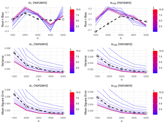
Figure 1: Setting 1 of Section 4.1 (Gaussian design and dense regression coefficients).

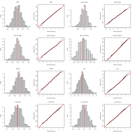
Figure 2: Setting 1 of Section 4.1 (Gaussian design and dense regression coefficients): Sampling distributions of the moment estimators and the parameter estimators, over 500 Monte Carlos are displayed for the case of $n=5000$.

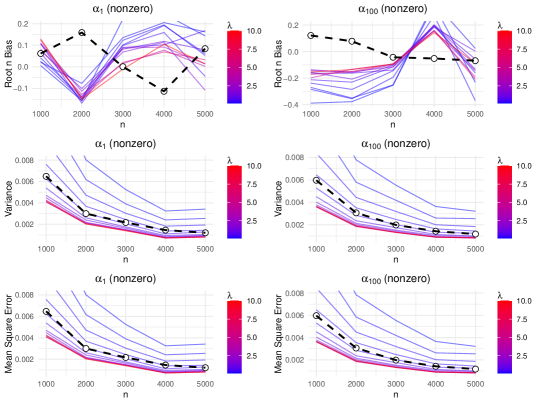
Figure 3: Setting 3 of Section 4.1 (Rademacher design and dense regression coefficients).

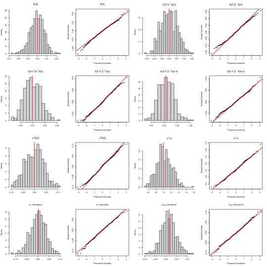
Figure 4: Setting 3 of Section 4.1 (Rademacher design and dense regression coefficients): Sampling distributions of the moment estimators and the parameter estimators, over 500 Monte Carlos are displayed for the case of $n=5000$.

4.2 Mean estimation with missing data under MAR

For the problem of estimating the mean of a response $Y$ under Model $\mathsf{MAR}$, we also consider several different settings. We first describe the common part of the DGP: the data is generated according to Model $\mathsf{MAR}$, with $\mathbf{X}_{i}\overset{\rm i.i.d.}{\sim}\mathrm{N}_{p}(\bm{0},\mathbf{I}_{p})$ for $i=1,\cdots,n$. We take ${\mathbb{E}}(A|\mathbf{X})=0.1+0.9\cdot\mathsf{expit}(\mathbf{X}^{\top}\bm{\alpha})$, as in Celentano and Wainwright (2023). Here the true value of the target parameter $\psi$ is 0 because $\mathbf{X}$ has mean zero. We take the outcome noise $\varepsilon\sim\mathrm{N}(0,\sigma^{2})$ with $\sigma=0.2$. The sample size varies from 100 to 10000. We compare our proposed MoM-based estimator $\widehat{\psi}$ with the two estimators proposed in Celentano and Wainwright (2023), respectively termed as “Oracle ASCW” and “Empirical SCA”. For these alternative estimators, initial estimates based on Ridge are also used, With the tuning parameter $\lambda$ taking 50 values ranging from $[0.01,10]$ with equal steps on a logarithmic scale. We refer readers to Celentano and Wainwright (2023) for the details of these two alternative estimators; here we simply implement the R code provided in the GitHub repository provided by the authors of Celentano and Wainwright (2023).

We also consider two different configurations for the regression coefficients $\bm{\alpha}$ and $\bm{\beta}$. In Setting 1 (Figures 5 – 6), we consider dense regression coefficients, where both $\bm{\alpha}$ and $\bm{\beta}$ are drawn i.i.d. coordinate-wise from $\mathrm{Uniform}([-\sqrt{3/p},\sqrt{3/p}])$. In Appendix H.3, we report results when changing the covariates distribution from Gaussian to $\mathbf{X}_{i,j}\overset{\rm i.i.d.}{\sim}\mathrm{Rad}(1/2)$ for $i=1,\cdots,n$ and $j=1,\cdots,p$. In Setting 2 (Figures 15 – 16), we consider sparse regression coefficients, where only $\alpha_{1}$ and $\beta_{1}$ are non-zero and are both equal to 1. Again, to save space, we defer the figures for Setting 2 to Appendix H.3.

As can be seen from Figures 5 and 15, the MoM-based estimators generally have lower $\sqrt{n}\times\mathrm{bias}$, variance, and mean squared error than the two estimators proposed in Celentano and Wainwright (2023), over a range of values of the tuning parameter $\lambda$, regardless of the configurations of the regression coefficients. Figures 6 and 16 display the histograms and normal quantile-quantile plots of the $U$-statistic-based moment estimators and the estimators of the target parameter $\psi$, together with $\lambda_{\alpha},\gamma_{\alpha}^{2},\gamma_{\alpha,\beta}$ (the byproducts of the system (11)). It is clear from these figures that the sampling distributions of both the $U$-statistic-based moment estimators and of the estimators of the target parameter $\psi$, together with $\lambda_{\alpha},\gamma_{\alpha}^{2},\gamma_{\alpha,\beta}$ (the byproducts of the system (11)), are close to the Gaussian distribution.

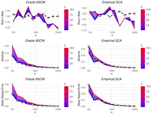
Figure 5: Simulation result for Setting 1 (dense regression coefficients) in Section 4.2. The two methods proposed in Celentano and Wainwright (2023) are plotted separately in two columns of the figure, with color gradients from blue to red representing the increasing value of the tuning parameter $\lambda$. The MoM-based estimators are plotted with white circles and dashed black lines.

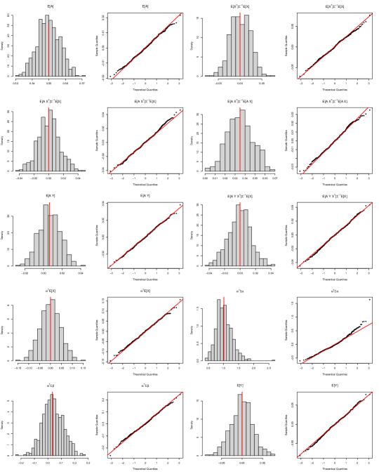
Figure 6: Simulation result for Setting 1 (dense regression coefficients) in Section 4.2: Sampling distributions of the moment estimators and the parameter estimators, over 500 Monte Carlos are displayed for the case of $n=5000$.

5 Discussion

This paper proposes Method-of-Moments (MoM) estimators of functionals of the regression coefficients in high-dimensional GLMs under the proportional asymptotic regime, in the most part assuming Gaussian designs with known population covariance matrix $\mathbf{\Sigma}$, following the current trend of literature. We demonstrate promising theoretical and numerical results about the MoM estimators. However, we emphasize that a more delicate comparison between our proposed approach and those based on de-biasing (Bellec, 2022; Celentano and Wainwright, 2023) is warranted in a future work: for instance, which estimator has better efficiency or which estimator is more readily extended to the case of unknown $\mathbf{\Sigma}$ or the case of violating sufficient conditions (e.g. Assumption $\mathsf{U}$) for universality.

5.1 Statistical Inference

The variance of the proposed estimator can be estimated by combining the variance estimators of $U$-statistics (for estimating the moments) (Liu et al., 2024) and the Delta Method. In particular, in Liu et al. (2024), we have shown that a particular bootstrapping scheme can be used to consistently estimate variances of the type of second-order $U$-statistic appeared as the moment estimators, which can be used to deliver asymptotically valid inference.

Another problem for statistical inference that is worth pursuing in future work relates to the potentially non-Gaussian limiting distribution. When the second-order degenerate part of our $U$-statistic estimators has variance of order $1/n^{2}$ instead of $p/n^{2}\asymp 1/n$, its asymptotic distribution is a Gaussian chaos distribution instead of a Gaussian distribution. It will be an interesting problem to investigate whether the bootstrap approach also delivers asymptotically valid inference in such a setting.

5.2 Unknown Population Covariance Matrix

In this paper, we assume that $\mathbf{\Sigma}$ is known, an assumption ubiquitously adopted in the current literature (see Section 1.2). Progress can be made when $\mathbf{\Sigma}$ is unknown, but for specific parameters such as linear forms or under more stringent dimension constraints for quadratic/bilinear forms (Su et al., 2023). We provide some further insights in Appendix D.

5.3 Single-Index Models (SIM) and Model Misspecification

Compared to GLMs, isotonic Single-Index Models (SIMs) (Kakade et al., 2011) offer a more flexible modeling option as they allow the link function to be unknown and nonparametric. To the best of our knowledge, Bellec (2022) is among the first to consider conducting statistical inference for functionals of regression coefficients in SIMs under proportional asymptotics. It will be interesting to extend our framework to single-index models but it requires estimating the link function from data, a complication that we plan to address in a separate paper. Finally, whenever parametric models such as GLMs are used, model misspecification is of potential concerns. The semiparametric partially nonlinear regression parameters considered in Vansteelandt and Dukes (2022), which reduce to functionals of regression coefficients when GLMs are correctly specified, can be a promising future avenue for our work.

Appendix A Preparatory Results

Lemma 8 (First- and Second-Order Stein’s lemma).

For $\mathbf{Z}\sim\mathrm{N}_{p}(\bm{0},\mathbf{I})$, we have for $f:{\mathbb{R}}^{p}\rightarrow{\mathbb{R}}$ that is differentiable,

$${\mathbb{E}}\left[\mathbf{Z}f(\mathbf{Z})\right]={\mathbb{E}}\left[\nabla f(\mathbf{Z})\right].$$

Similarly, we have for $h:{\mathbb{R}}^{p}\rightarrow{\mathbb{R}}$ and $f:{\mathbb{R}}^{p}\rightarrow{\mathbb{R}}$ that are twice differentiable,

$${\mathbb{E}}\left[\left(\mathbf{Z}\mathbf{Z}^{\top}-\mathbf{I}\right)h(\mathbf{Z})\right] ={\mathbb{E}}\left[\nabla^{2}h(\mathbf{Z})\right],$$

$${\mathbb{E}}\left[\left(\mathbf{Z}^{\top}f(\mathbf{Z})-\mathsf{div}f(\mathbf{Z})\right)^{2}\right] ={\mathbb{E}}\left[\|f(\mathbf{Z})\|^{2}+\mathsf{trace}\left(\nabla^{2}f(\mathbf{Z})\right)\right].$$

Corollary 1.

For $\mathbf{X}\sim\mathrm{N}_{p}(\bm{\mu},\mathbf{\Sigma})$, we have, for $f:{\mathbb{R}}^{p}\rightarrow{\mathbb{R}}$ that is differentiable,

$${\mathbb{E}}\left[\mathbf{X}f(\mathbf{X})\right]=\bm{\mu}{\mathbb{E}}[f(\mathbf{X})]+\mathbf{\Sigma}{\mathbb{E}}[\nabla f(\mathbf{X})].$$

In addition, we have, for $\mathbf{f}:{\mathbb{R}}^{p}\rightarrow{\mathbb{R}}^{p}$ that is coordinate-wisely differentiable,

$${\mathbb{E}}[\mathbf{X}^{\top}\mathbf{f}(\mathbf{X})]=\bm{\mu}^{\top}{\mathbb{E}}[\mathbf{f}(\mathbf{X})]+\mathsf{trace}\left[\mathbf{\Sigma}{\mathbb{E}}[\nabla\mathbf{f}(\mathbf{X})]\right].$$ (17)

Similarly, we have for $h:{\mathbb{R}}^{p}\rightarrow{\mathbb{R}}$ that is twice differentiable,

$${\mathbb{E}}\left[\left(\mathbf{X}\mathbf{X}^{\top}-\mathbf{\Sigma}\right)h(\mathbf{X})\right]=\bm{\mu}\bm{\mu}^{\top}{\mathbb{E}}[h(\mathbf{X})]+\bm{\mu}(\mathbf{\Sigma}{\mathbb{E}}[\nabla h(\mathbf{X})])^{\top}+(\mathbf{\Sigma}{\mathbb{E}}[\nabla h(\mathbf{X})])\bm{\mu}^{\top}+\mathbf{\Sigma}{\mathbb{E}}[\nabla^{2}h(\mathbf{X})]\mathbf{\Sigma}.$$ (18)

Proof.

The proof for the first statement is trivial and hence omitted. Let $\mathbf{Z}\sim\mathrm{N}_{p}(\bm{0},\mathbf{I})$ then $\mathbf{X}\overset{d}{=}\mathbf{\Sigma}^{1/2}\mathbf{Z}+\bm{\mu}$.

$$\ {\mathbb{E}}\left[\left(\mathbf{X}\mathbf{X}^{\top}-\mathbf{\Sigma}\right)h(\mathbf{X})\right]$$

$$= \ {\mathbb{E}}\left[\left((\mathbf{X}-\bm{\mu}+\bm{\mu})(\mathbf{X}-\bm{\mu}+\bm{\mu})^{\top}-\mathbf{\Sigma}\right)h(\mathbf{X})\right]$$

$$= \ \bm{\mu}\bm{\mu}^{\top}{\mathbb{E}}[h(\mathbf{X})]+\bm{\mu}{\mathbb{E}}\left[(\mathbf{X}-\bm{\mu})^{\top}h(\mathbf{X})\right]+{\mathbb{E}}\left[(\mathbf{X}-\bm{\mu})h(\mathbf{X})\right]\bm{\mu}^{\top}+{\mathbb{E}}\left[\left\{(\mathbf{X}-\bm{\mu})(\mathbf{X}-\bm{\mu})^{\top}-\mathbf{\Sigma}\right\}h(\mathbf{X})\right]$$

$$= \ \bm{\mu}\bm{\mu}^{\top}{\mathbb{E}}[h(\mathbf{X})]+\bm{\mu}(\mathbf{\Sigma}{\mathbb{E}}[\nabla h(\mathbf{X})])^{\top}+(\mathbf{\Sigma}{\mathbb{E}}[\nabla h(\mathbf{X})])\bm{\mu}^{\top}+\mathbf{\Sigma}^{1/2}{\mathbb{E}}\left[(\mathbf{Z}\mathbf{Z}^{\top}-\mathbf{I})h(\mathbf{\Sigma}^{1/2}\mathbf{Z}+\bm{\mu})\right]\mathbf{\Sigma}^{1/2}$$

$$= \ \bm{\mu}\bm{\mu}^{\top}{\mathbb{E}}[h(\mathbf{X})]+\bm{\mu}(\mathbf{\Sigma}{\mathbb{E}}[\nabla h(\mathbf{X})])^{\top}+(\mathbf{\Sigma}{\mathbb{E}}[\nabla h(\mathbf{X})])\bm{\mu}^{\top}+\mathbf{\Sigma}{\mathbb{E}}[\nabla^{2}h(\mathbf{X})]\mathbf{\Sigma}.$$

∎

Corollary 2.

For $Z\sim\mathrm{N}(\lambda,\gamma^{2})$, given a twice-differentiable function $f:{\mathbb{R}}\rightarrow{\mathbb{R}}$, we have

$${\mathbb{E}}f(Z)(Z-\lambda)^{2}=\gamma^{2}{\mathbb{E}}f(Z)+(\gamma^{2})^{2}{\mathbb{E}}f^{\prime\prime}(Z).$$

Proof.

Repeatedly applying Lemma 8, we have

$${\mathbb{E}}f(Z)(Z-\lambda)^{2} ={\mathbb{E}}f(Z)(Z-\lambda)(Z-\lambda)$$

$$=\gamma^{2}{\mathbb{E}}\{f^{\prime}(Z)(Z-\lambda)+f(Z)\}$$

$$=\gamma^{2}{\mathbb{E}}f(Z)+(\gamma^{2})^{2}{\mathbb{E}}f^{\prime\prime}(Z).$$

∎

As our proposed MoM-based estimators critically rely on inverting a nonlinear map (generally without an analytic form), we also need the following fundamental result about smooth functions, particularly in Appendix F.

Lemma 9 (Inverse function theorem (Theorem C.34 of Lee (2012))).

Suppose ${\mathcal{R}}$ and ${\mathcal{M}}$ are open sets of ${\mathbb{R}}^{k}$ for some positive integer $k$ and $\Psi:{\mathcal{R}}\rightarrow{\mathcal{M}}$ is a smooth function. If $\nabla\Psi$ is invertible over ${\mathcal{R}}$, then $\Psi$ is a diffeomorphism.

Appendix B Proof for the system of moment equations for GLM

After the preparation in the previous section, we are ready to prove the first part of Lemma 3. We only need to verify (6c), (6d), and (6f) of (6).

Regarding (6c), we can simply apply Corollary 1 and obtain:

$$m_{\mathbf{X}Y,\mathbf{X}} ={\mathbb{E}}[\phi(\bm{\beta}^{\top}\mathbf{X})\mathbf{X}^{\top}]\mathbf{\Sigma}^{-1}{\mathbb{E}}[\mathbf{X}]={\mathbb{E}}[\phi(\bm{\beta}^{\top}\mathbf{X})]\bm{\mu}^{\top}\mathbf{\Sigma}^{-1}\bm{\mu}+{\mathbb{E}}[\phi^{\prime}(\bm{\beta}^{\top}\mathbf{X})]\bm{\beta}^{\top}\mathbf{\Sigma}\mathbf{\Sigma}^{-1}\bm{\mu}$$

$$={\mathbb{E}}[Y]\bm{\mu}^{\top}\mathbf{\Sigma}^{-1}\bm{\mu}+{\mathbb{E}}[\phi^{\prime}(\bm{\beta}^{\top}\mathbf{X})]\bm{\beta}^{\top}\bm{\mu}$$

$$=m_{Y}\cdot m_{\mathbf{X},2}+\mathrm{f}_{1}(\lambda_{\beta},\gamma_{\beta}^{2})\cdot\lambda_{\beta}.$$

The derivations of (6d) and (6f) follow the same strategy, hence omitted.

Appendix C Proof for Universality

To extend the results from Gaussian designs to non-Gaussian designs, the following lemma from Chatterjee (2006) (also see Han and Shen (2023)) is pivotal.

Lemma 10.

Let $\bar{X}\coloneqq(X_{1},\cdots,X_{p})$ and $\bar{Y}\coloneqq(Y_{1},\cdots,Y_{p})$ be two collections of random vectors with independent coordinates and matching first and second moments: ${\mathbb{E}}[X_{j}^{k}]={\mathbb{E}}[Y_{j}^{k}]$ for $j=1,\cdots,p$ and $k\in\{1,2\}$. For any three-time differentiable function $f$,

$$\left|{\mathbb{E}}f(\bar{X})-{\mathbb{E}}f(\bar{Y})\right|\leq\sum_{j=1}^{p}\max_{Z_{j}\in\{X_{j},Y_{j}\}}\left|{\mathbb{E}}\int_{0}^{Z_{j}}\partial^{3}_{j}f(X_{1},\cdots,X_{j-1},t,Y_{j+1},\cdots,Y_{p})(Z_{j}-t)^{2}{\mathrm{d}}t\right|,$$ (19)

where $\partial^{3}_{j}f$ denotes the third-derivative of $f$ with respect to the $j$-th argument.

Lemma 11.

Suppose that Assumptions $\mathsf{L}$ and $\mathsf{U}$ hold and ${\mathbb{M}}$ is a n.n.s.d. matrix such that $M^{-1}\leq\lambda_{\min}({\mathbb{M}})\leq\lambda_{\max}({\mathbb{M}})\leq M$. We then have the following assertions:

1. ${\mathbb{E}}(\bm{\beta}^{\top}\mathbf{X}\phi(\bm{\alpha}^{\top}\mathbf{X}))=\bm{\beta}^{\top}\mathbf{\Sigma}\bm{\alpha}{\mathbb{E}}(\phi^{\prime}(\mathbf{Y}^{\top}\bm{\alpha}))+\bm{\beta}^{\top}\bm{\mu}{\mathbb{E}}(\phi(\mathbf{Y}^{\top}\bm{\alpha}))+O(p^{-3/4})$;

2. ${\mathbb{E}}(\phi(\bm{\alpha}^{\top}\mathbf{X}))={\mathbb{E}}(\phi(\bm{\alpha}^{\top}\mathbf{Y}))+O(p^{-3/4})$.

3. $\{Y_{i},\mathbf{X}_{i}\}_{i=1}^{n}\overset{\rm i.i.d.}{\sim}{\mathbb{P}}$ with ${\mathbb{E}}(Y|\mathbf{X})=\phi(\bm{\alpha}^{\top}\mathbf{X})$ and let $T_{n}={\mathbb{U}}_{n,2}(Y_{1}\mathbf{X}_{1}^{\top}{\mathbb{M}}\mathbf{X}_{2}Y_{2})$. Then $\mathsf{var}(T_{n})=O(1/n+p/n^{2})$ if ${\mathbb{E}}(\sigma^{4}(\mathbf{X}))<\infty$ with $\sigma^{2}(\mathbf{X})=\mathsf{var}(Y|\mathbf{X})$.

Proof.

We prove assertion 1 and the proof of 2 follows by parallel arguments with obvious modifications. To prove 1, we first start with the case $\mathbf{\Sigma}=\mathbf{I}$ and $\bm{\mu}=\mathbf{0}$ and subsequently provide the details necessary for extending to the general mean and covariance cases. To this end define the function $f:\mathbb{R}^{p}\rightarrow\mathbb{R}$ as $f(\bm{\omega})=\bm{\omega}^{\top}\bm{\beta}\phi(\bm{\omega}^{\top}\bm{\alpha})$ for $\bm{\omega}=(\omega,\ldots,\omega_{p})^{\top}\in{\mathbb{R}}^{p}$. Therefore it is clear that

$$\frac{\partial^{3}}{\partial\omega_{j}^{3}}f(\bm{\omega}) =\bm{\omega}^{\top}\bm{\beta}\alpha_{j}^{3}\phi^{(3)}(\bm{\omega}^{\top}\bm{\alpha})+3\beta_{j}\alpha_{j}^{2}\phi^{(2)}(\bm{\omega}^{\top}\bm{\alpha}).$$

Therefore by Lemma 10

$$|{\mathbb{E}}(\mathbf{X}^{\top}\bm{\beta}\phi(\mathbf{X}^{\top}\alpha))-{\mathbb{E}}(\mathbf{Y}^{\top}\bm{\beta}\phi(\mathbf{Y}^{\top}\alpha))|$$

$$\leq\sum_{j=1}^{p}\max_{V_{j}\in\{X_{j},Y_{j}\}}\left|{\mathbb{E}}\int_{0}^{V_{j}}\frac{\partial^{3}}{\partial\omega_{j}^{3}}f(X_{1},\ldots,X_{j-1},t,Y_{j+1},\ldots,Y_{p})(Z_{j}-t)^{2}dt\right|$$

$$\leq T_{1}+T_{2},$$

where $T_{1},T_{2}$ respect the decomposition of $\frac{\partial^{3}}{\partial\omega_{j}^{3}}f(\bm{\omega})$ after applying triangle inequality to the display above. We first consider $T_{1}$ as follows by defining $W_{l,j}(\kappa,t)=\kappa(X_{l}\mathbbm{1}(l<j)+Y_{l}\mathbbm{1}(l>j)+t\mathbbm{1}(l=j))$

$$T_{1} =\sum_{j=1}^{p}|\alpha_{j}^{3}|\max\limits_{V_{j}\in\{X_{j},Y_{j}\}}\left|{\mathbb{E}}\int_{0}^{V_{j}}\sum_{l=1}^{p}W_{l,j}(\beta_{l},t)\phi^{(3)}\left(\sum_{l=1}^{p}W_{l,j}(\alpha_{l},t)\right)(V_{j}-t)^{2}{\mathrm{d}}t\right|.$$

Now by Cauchy-Schwarz inequality,

$$\begin{split}\ &\left|{\mathbb{E}}\int_{0}^{V_{j}}\sum_{l\neq j}W_{l,j}(\beta_{l},t)\phi^{(3)}\left(\sum_{l=1}^{p}W_{l,j}(\alpha_{l},t)\right)(V_{j}-t)^{2}{\mathrm{d}}t\right|\\ &\leq\left(\left|{\mathbb{E}}\int_{0}^{V_{j}}\left\{\phi^{(3)}\left(\sum_{l=1}^{p}W_{l,j}(\alpha_{l},t)\right)\right\}^{2}{\mathrm{d}}t\right|\right)^{1/2}\left(\left|{\mathbb{E}}\int_{0}^{V_{j}}\left\{\sum_{l\neq j}W_{l,j}(\beta_{l},t)(V_{j}-t)^{2}\right\}^{2}{\mathrm{d}}t\right|\right)^{1/2}.\end{split}$$ (20)

We analyze the two terms of the product in the last display as follows.

$$\left|{\mathbb{E}}\int_{0}^{V_{j}}\left\{\phi^{(3)}\left(\sum_{l=1}^{p}W_{l,j}(\alpha_{l},t)\right)\right\}^{2}{\mathrm{d}}t\right|$$

$$\leq\left|{\mathbb{E}}\int_{0}^{V_{j}}\left\{\phi^{(3)}\left(\sum_{l\neq j}^{p}W_{l,j}(\alpha_{l},0)\right)\right\}^{2}{\mathrm{d}}t\right|+|\alpha_{j}|\left|{\mathbb{E}}\int_{0}^{V_{j}}tf_{\phi}\left(\sum_{l\neq j}^{p}W_{l,j}(\alpha_{l},0)+\alpha_{j}\chi(t)\right){\mathrm{d}}t\right|$$

$$=|\alpha_{j}|\left|{\mathbb{E}}\int_{0}^{V_{j}}tf_{\phi}\left(\sum_{l\neq j}^{p}W_{l,j}(\alpha_{l},0)+\alpha_{j}\chi(t)\right){\mathrm{d}}t\right|$$

where $\chi(t)$ is a $\sum_{l\neq j}^{p}W_{l,j}(\alpha_{l},0)$-measurable quantity between $\sum_{l\neq j}^{p}W_{l,j}(\alpha_{l},0)$ and $t$ by the exact form of Taylor remainder theorem, and we used the facts that $W_{l,j}(\kappa,t)=W_{l,j}(\kappa,0)$ for $l\neq j$, ${\mathbb{E}}(V_{j})=0$ and $V_{j}\perp\sum_{l\neq j}W_{l,j}(\alpha_{l},0)$, and also the short-hand notation $f_{\phi}(\cdot)\coloneqq\{\phi^{(3)}(\cdot)^{2}\}^{\prime}$. Now note that by the property of the function $\phi$ and the range of integration over $t$,

$$\left|{\mathbb{E}}\int_{0}^{V_{j}}tf_{\phi}\left(\sum_{l\neq j}^{p}W_{l,j}(\alpha_{l},0)+\alpha_{j}\chi(t)\right){\mathrm{d}}t\right|$$

$$\leq 2\left|{\mathbb{E}}\int_{0}^{V_{j}}|t|\exp\left\{2\left(\sum_{l\neq j}^{p}W_{l,j}(\alpha_{l},0)+\alpha_{j}\chi(t)\right)^{2}f\left(\sum_{l\neq j}^{p}W_{l,j}(\alpha_{l},0)+\alpha_{j}\chi(t)\right)\right\}{\mathrm{d}}t\right|$$

$$\leq 2\left|{\mathbb{E}}\int_{0}^{V_{j}}|V_{j}|\exp\left\{2\left(\sum_{l\neq j}^{p}W_{l,j}(\alpha_{l},0)+\alpha_{j}\chi(t)\right)^{2}f\left(\sum_{l\neq j}^{p}W_{l,j}(\alpha_{l},0)+\alpha_{j}\chi(t)\right)\right\}{\mathrm{d}}t\right|.$$

Next, we again note that by the exact form of Taylor remainder theorem it is clear that $\chi(t)$ is $\sum_{l\neq j}^{p}W_{l,j}(\alpha_{l},0)$-measurable and hence

$$\exp\left\{2\left(\sum_{l\neq j}^{p}W_{l,j}(\alpha_{l},0)+\alpha_{j}\chi(t)\right)^{2}f\left(\sum_{l\neq j}^{p}W_{l,j}(\alpha_{l},0)+\alpha_{j}\chi(t)\right)\right\}\perp V_{j}.$$

Now by direct calculations and the fact that $\max_{l=1}^{p}\|V_{l}\|_{\psi_{2}}\leq M$, $|\chi(t)|\leq|V_{j}|$ and $\lim_{|x|\rightarrow\infty}f(x)=0$ it is straightforward to verify that

$$2\left|{\mathbb{E}}\int_{0}^{V_{j}}|V_{j}|\exp\left\{2\left(\sum_{l\neq j}^{p}W_{l,j}(\alpha_{l},0)+\alpha_{j}\chi(t)\right)^{2}f\left(\sum_{l\neq j}^{p}W_{l,j}(\alpha_{l},0)+\alpha_{j}\chi(t)\right)\right\}{\mathrm{d}}t\right|$$

is bounded. Similarly using the fact that $\|\sum_{l\neq j}W_{l,j}(\beta_{l},t)\|_{\psi_{2}}\leq M$ and it is independent of $V_{j}$ which also has $\psi_{2}$-norm bounded by $M$ one has by straightforward algebra that

$$\left|\int_{0}^{V_{j}}{\mathbb{E}}\left\{\sum_{l\neq j}W_{l,j}(\beta_{l},t)(V_{j}-t)^{2}\right\}^{2}{\mathrm{d}}t\right|$$

is bounded as well. Consequently there exists a constant $C(M)$ depending on $M$ such that

$$\left|{\mathbb{E}}\int_{0}^{V_{j}}\sum_{l\neq j}W_{l,j}(\beta_{l},t)\phi^{(3)}\left(\sum_{l=1}^{p}W_{l,j}(\alpha_{l},t)\right)(V_{j}-t)^{2}{\mathrm{d}}t\right|\leq C(M)|\alpha_{j}|.$$

Therefore for some constant $C^{\prime}(M)$ depending on $M$

$$T_{1} \leq C^{\prime}(M)\sum_{j=1}^{p}|\alpha_{j}|^{7/2}=O(p^{-3/4}).$$

By a parallel argument, it is easy to show that for some constant $C^{\prime\prime}(M)$ depending on $M$

$$T_{2} \leq C^{\prime\prime}(M)\sum_{j=1}^{p}|\beta_{j}||\alpha_{j}|^{5/2}=O(p^{-3/4}).$$

This completes the proof of the first statement. The second statement follows directly from the same proof strategy and is thus omitted. It is noteworthy that if ${\mathbb{E}}(V_{j})=\mu_{j}$ is not necessarily 0 when $\bm{\mu}\neq\bm{0}$, we can still apply the same arguments by further controlling the first term on the LHS of (20) by leveraging the assumption on $\bm{\mu}$ imposed in Assumption $\mathsf{D}$. When $\mathbf{\Sigma}\neq\mathbf{I}$, the above proof also goes through by renaming $\bm{\alpha}$ and $\bm{\beta}$ as $\mathbf{\Sigma}^{1/2}\bm{\alpha}$ and $\mathbf{\Sigma}^{1/2}\bm{\beta}$.

Next we prove the claim 3 that for $T_{n}={\mathbb{U}}_{n,2}(Y_{1}\mathbf{X}_{1}^{\top}{\mathbb{M}}\mathbf{X}_{2}Y_{2})$ we have that $\mathsf{var}(T_{n})=O(1/n+p/n^{2})$ when $\mathbf{X}=\mathbf{\Sigma}^{1/2}\mathbf{Z}+\bm{\mu}$. We note that by Assumption $\mathsf{D}$ it is enough to consider the case $\bm{\mu}=\mathbf{0}$, which we assume henceforth. Thereafter, let $T_{1n}$ and $T_{2n}$ denote the first and second order term of the Hoeffding decomposition of $T_{n}$.

We first show that $\mathsf{var}(T_{1n})=O(1/n)$. To show this, note that with $\upsilon_{{\mathbb{M}}}\coloneqq{\mathbb{M}}{\mathbb{E}}(\mathbf{X}Y)={\mathbb{M}}{\mathbb{E}}(\mathbf{X}\phi(\mathbf{X}^{\top}\bm{\beta}))$ we have that

$$\mathsf{var}(T_{1n}) =\frac{1}{n}\mathsf{var}\left(Y\mathbf{X}^{\top}\upsilon_{{\mathbb{M}}}\right)$$

$$=\frac{1}{n}\mathsf{var}(\phi(\mathbf{X}^{\top}\bm{\beta})\mathbf{X}^{\top}\upsilon_{{\mathbb{M}}})+\frac{1}{n}{\mathbb{E}}(\sigma^{2}(\mathbf{X})(\upsilon_{{\mathbb{M}}}^{\top}\mathbf{X})^{2})$$

Now since $\|\upsilon_{{\mathbb{M}}}^{\top}\mathbf{X}\|_{\psi_{2}}\leq M\|\upsilon_{{\mathbb{M}}}\|_{2}$, $\|\upsilon_{{\mathbb{M}}}\|_{2}^{2}\leq\lambda_{\max}^{2}({\mathbb{M}})\|{\mathbb{E}}(\mathbf{X}^{\top}\phi(\mathbf{X}^{\top}\bm{\beta}))\|_{2}^{2}$. But $\mathbf{X}^{\top}\mathbf{\Sigma}^{-1}{\mathbb{E}}(\mathbf{X}\phi(\mathbf{X}^{\top}\bm{\beta}))=\mathrm{Proj}_{L_{2}({\mathbb{P}})}\left(\phi(\mathbf{X}^{\top}\bm{\beta})|V\right)$ where $V=\mathrm{Span}(\mathbf{X})$. Therefore by the length contraction property of projection, we have

$$\|\mathbf{X}^{\top}\mathbf{\Sigma}^{-1}{\mathbb{E}}(\mathbf{X}\phi(\mathbf{X}^{\top}\bm{\beta}))\|_{L_{2}({\mathbb{P}})}^{2}\leq\|\phi(\mathbf{X}^{\top}\bm{\beta})\|_{L_{2}({\mathbb{P}})}^{2}.$$

However,

$$\|\mathbf{X}^{\top}\mathbf{\Sigma}^{-1}{\mathbb{E}}(\mathbf{X}\phi(\mathbf{X}^{\top}\bm{\beta}))\|_{L_{2}({\mathbb{P}})}^{2} ={\mathbb{E}}(\mathbf{X}^{\top}\phi(\mathbf{X}^{\top}\bm{\beta}))\mathbf{\Sigma}^{-1}{\mathbb{E}}(\mathbf{X}\phi(\mathbf{X}^{\top}\bm{\beta}))$$

$$\geq\lambda_{\max}^{-1}(\mathbf{\Sigma})\|{\mathbb{E}}(\mathbf{X}\phi(\mathbf{X}^{\top}\bm{\beta}))\|_{2}^{2}.$$

Therefore

$$\|\upsilon_{{\mathbb{M}}}\|_{2}^{2}\leq\lambda_{\max}^{2}({\mathbb{M}})\|{\mathbb{E}}(\mathbf{X}^{\top}\phi(\mathbf{X}^{\top}\bm{\beta}))\|_{2}^{2}\leq\lambda_{\max}(\mathbf{\Sigma})\lambda_{\max}({\mathbb{M}})\|\phi(\mathbf{X}^{\top}\bm{\beta})\|_{L_{2}({\mathbb{P}})}^{2}<\infty.$$

Thus we have

$$\mathsf{var}(\phi(\mathbf{X}^{\top}\bm{\beta})\mathbf{X}^{\top}\upsilon_{{\mathbb{M}}}) \leq{\mathbb{E}}^{1/2}\left(\phi^{4}(\mathbf{X}^{\top}\bm{\beta})\right){\mathbb{E}}^{1/2}\left((\upsilon_{{\mathbb{M}}}^{\top}\mathbf{X})^{4}\right)<\infty,$$

$${\mathbb{E}}(\sigma^{2}(\mathbf{X})(\upsilon_{{\mathbb{M}}}^{\top}\mathbf{X})^{2}) \leq{\mathbb{E}}^{1/2}\left(\sigma^{4}(\mathbf{X})\right){\mathbb{E}}^{1/2}\left((\upsilon_{{\mathbb{M}}}^{\top}\mathbf{X})^{4}\right)<\infty.$$

This completes the proof of the fact that $\mathsf{var}(T_{1n})=O(1/n)$.

Wring $\mathbf{Z}_{l,M}={\mathbb{M}}^{1/2}\mathbf{\Sigma}^{1/2}\mathbf{Z}_{l}$, we note that $\|\mathbf{X}_{1}^{\top}{\mathbb{M}}\mathbf{X}_{2}\|^{2}_{\psi_{1}}\leq 2\|\|\mathbf{Z}_{1,{\mathbb{M}}}+\mathbf{Z}_{2,{\mathbb{M}}}\|_{2}^{2}\|_{\psi_{1}}^{2}+2\|\|\mathbf{Z}_{1,{\mathbb{M}}}-\mathbf{Z}_{2,{\mathbb{M}}}\|_{2}^{2}\|_{\psi_{1}}^{2}\leq 16\sum_{j=1}^{p}\|Z_{1,M}^{2}(j)\|_{\psi_{1}}^{2}\leq 16M^{2}p$ for some $C$ depending on $M$. Therefore for any $k\in\mathbb{N}$ we have ${\mathbb{E}}\left\{\mathbf{X}_{1}^{\top}{\mathbb{M}}\mathbf{X}_{2}\right\}^{k}\leq C^{\prime}(M)p^{k/2}$ for some $C^{\prime}$ depending on $M$. Consequently, we have by Jensen’s inequality

$$\mathsf{var}(T_{2n}) \leq\frac{C}{n^{2}}{\mathbb{E}}\left(Y_{i}^{2}Y_{j}^{2}(\mathbf{X}_{i}^{\top}{\mathbb{M}}\mathbf{X}_{j})^{2}\right)$$

$$=\frac{C}{n^{2}}{\mathbb{E}}\left[\left\{\sigma^{2}(\mathbf{X}_{1})\sigma^{2}(\mathbf{X}_{2})+2\sigma^{2}(\mathbf{X}_{1})\phi^{2}(\mathbf{X}_{2}^{\top}\bm{\beta})+\phi^{2}(\mathbf{X}_{1}^{\top}\bm{\beta})\phi^{2}(\mathbf{X}_{2}^{\top}\bm{\beta})\right\}\left\{\mathbf{X}_{1}^{\top}{\mathbb{M}}\mathbf{X}_{2}\right\}^{2}\right]$$

$$\leq\frac{C}{n^{2}}{\mathbb{E}}^{1/2}\left[\left\{\sigma^{2}(\mathbf{X}_{1})\sigma^{2}(\mathbf{X}_{2})+2\sigma^{2}(\mathbf{X}_{1})\phi^{2}(\mathbf{X}_{2}^{\top}\bm{\beta})+\phi^{2}(\mathbf{X}_{1}^{\top}\bm{\beta})\phi^{2}(\mathbf{X}_{2}^{\top}\bm{\beta})\right\}^{2}\right]{\mathbb{E}}^{1/2}\left[\left(\mathbf{X}_{1}^{\top}{\mathbb{M}}\mathbf{X}_{2}\right)^{4}\right]$$

$$\leq\frac{C^{\prime\prime}(M)p}{n^{2}},$$

for some $C^{\prime\prime}$ depending on $M$. This completes the proof of the lemma. ∎

With Lemma 11, we are ready to prove Lemma 4, and as a direct corollary of Lemma 4, Lemma 2.

Proof of Lemma 4.

It is easy to see that to show Lemma 4, it is sufficient to apply Lemma 11 to each individual moment equation in (6) separately. In particular, the proof is complete once one observes that the LHS of each identity in (6) either has the form of ${\mathbb{E}}(\bm{\beta}^{\top}\mathbf{X}\phi(\bm{\alpha}^{\top}\mathbf{X}))$ or ${\mathbb{E}}(\phi(\bm{\alpha}^{\top}\mathbf{X}))$ with appropriately chosen $\bm{\alpha}$, $\bm{\beta}$, and $\phi$. ∎

Appendix D Unknown Population Covariance Matrix

D.1 Linear Models

For notational convenience, we take $\bm{\mu}=\bm{0}$ so the population covariance matrix $\mathbf{\Sigma}$ is identical to the population Gram matrix ${\mathbb{E}}[\mathbf{X}\mathbf{X}^{\top}]\equiv\mathbf{\Sigma}+\bm{\mu}\bm{\mu}^{\top}$. But we consider the situation where the statistician does not know $\bm{\mu}=\bm{0}$. Under the linear model with homoscedastic variance, for estimating the linear and quadratic forms $\lambda_{\beta}=\bm{\beta}^{\top}\bm{\mu}$ and $\gamma_{\beta}^{2}=\bm{\beta}^{\top}\mathbf{\Sigma}\bm{\beta}$, we consider the following estimators without knowing $\mathbf{\Sigma}$ but under the assumption that the empirical covariance matrix $\widehat{\mathbf{\Sigma}}$ is invertible:

$$\widehat{\lambda}_{\beta} \coloneqq{\mathbb{U}}_{n,1}[Y]\equiv\frac{1}{n}\mathbf{1}^{\top}\mathbf{Y},$$

$$\widehat{\gamma}_{\beta}^{2} \coloneqq\frac{1}{n-p}\left\{\mathbf{Y}^{\top}\left({\mathbb{H}}-\frac{p}{n}\mathbf{I}\right)\mathbf{Y}\right\},$$

where we denote ${\mathbb{X}}\coloneqq(\mathbf{X}_{1},\cdots,\mathbf{X}_{n})^{\top}$ as the $n\times p$ design matrix, ${\mathbb{H}}\coloneqq{\mathbb{X}}({\mathbb{X}}^{\top}{\mathbb{X}})^{-1}{\mathbb{X}}$ as the “hat” projection matrix, $\mathbf{Y}\coloneqq(Y_{1},\cdots,Y_{n})^{\top}\in{\mathbb{R}}^{n}$ as the vector collecting the responses over all the subjects, and $\mathbf{1}$ as the $n$-dimensional all-1 vector. The unbiasedness, $\sqrt{n}$-consistency and CAN of $\widehat{\lambda}_{\beta}$ is trivial. The unbiasedness, $\sqrt{n}$-consistency and CAN of $\widehat{\gamma}_{\beta}^{2}$ follow directly from Theorem 1 of Guo and Cheng (2022). $\widehat{\gamma}_{\beta}^{2}$ can also be viewed as approximating a second-order $U$-statistic with the removed diagonal part approximated by $\frac{1}{n}\mathbf{Y}^{\top}\cdot\frac{p}{n-p}\mathbf{I}\cdot\mathbf{Y}$.

For a single coordinate $\beta_{j}$, we consider the following estimator:

$$\widehat{\beta}_{j}=e_{j}^{\top}({\mathbb{X}}^{\top}{\mathbb{X}})^{-1}{\mathbb{X}}^{\top}\mathbf{Y}.$$

First, $\widehat{\beta}_{j}$ is obviously conditionally, and hence unconditionally, unbiased. We only need to control its variance:

$$\mathsf{var}(\widehat{\beta}_{j}) ={\mathbb{E}}[\mathsf{var}(\widehat{\beta}_{j}|{\mathbb{X}})]+\mathsf{var}({\mathbb{E}}[\mathsf{var}(\widehat{\beta}_{j})|{\mathbb{X}}])$$

$$={\mathbb{E}}[\mathsf{var}(e_{j}^{\top}({\mathbb{X}}^{\top}{\mathbb{X}})^{-1}{\mathbb{X}}^{\top}\mathbf{Y}|{\mathbb{X}})].$$

Then

$$\mathsf{var}(e_{j}^{\top}({\mathbb{X}}^{\top}{\mathbb{X}})^{-1}{\mathbb{X}}^{\top}\mathbf{Y}|{\mathbb{X}})=\sigma^{2}e_{j}^{\top}({\mathbb{X}}^{\top}{\mathbb{X}})^{-1}e_{j}.$$

So

$$\mathsf{var}(\widehat{\beta}_{j})=\sigma^{2}e_{j}^{\top}{\mathbb{E}}[({\mathbb{X}}^{\top}{\mathbb{X}})^{-1}]e_{j}.$$

A common theme of the above estimators is the reliance on the correctness of the homoscedastic linear model. It remains to be seen if a similar strategy can be applied to estimating the moments involved in system of equations such as (6) for GLMs or more general nonlinear models, when $\mathbf{\Sigma}$ is unknown and $p<n$.

D.2 Generalized Linear Models

In this section, we prove Proposition 3 by taking $n/2$ as $n$ to avoid notation clutter. As a result, the notation in this proof will follow that in Section 2.2 only. We only need to show that $\widehat{\gamma}_{\beta}^{2}$, as defined in Section 2.2, is a $\sqrt{n}$-consistent estimator of $\gamma_{\beta}^{2}$.

We first make the following important observation, which is another important implication of the Gaussian design (Couillet and Liao, 2022; Dereziński et al., 2021).

Lemma 12.

Under Assumption $\mathsf{G_{0}}$, if $n>p+3$,

$$\widetilde{\mathbf{\Sigma}}\sim\mathsf{Wishart}_{p}(n^{-1}\mathbf{\Sigma},n),\widetilde{\mathbf{\Sigma}}^{-1}\equiv\widetilde{\mathbf{\Omega}}\sim\mathsf{Wishart}_{p}^{-1}(n\mathbf{\Sigma}^{-1}\equiv n\mathbf{\Omega},n)$$

where $\mathsf{Wishart}_{p}(\mathbf{V},m)$ and $\mathsf{Wishart}_{p}^{-1}(\mathbf{V},m)$, respectively, denote the $p$-dimensional Wishart and Inverse-Wishart distributions with $m$ degrees-of-freedom and scale matrix $\mathbf{V}$. Thus

$${\mathbb{E}}(\widetilde{\mathbf{\Sigma}}^{-1})\equiv{\mathbb{E}}(\widetilde{\mathbf{\Omega}})\equiv\frac{n}{n-p-1}\mathbf{\Sigma}^{-1}$$ (21)

and for $i,j\in[p]$,

$$\mathsf{cov}\left(\widetilde{\omega}_{i,j},\widetilde{\omega}_{k,l}\right)=\frac{2n^{2}\omega_{i,j}\omega_{k,l}+(n-p-1)n^{2}(\omega_{i,k}\omega_{j,l}+\omega_{i,l}\omega_{k,j})}{(n-p)(n-p-1)^{2}(n-p-3)}$$ (22)

It is easy to see that $\widehat{m}_{\mathbf{X}Y,2}$ is an unbiased estimator of $m_{\mathbf{X}Y,2}$. We are now left to control its variance. Under Assumption $\mathsf{C}$, the prefactor of (5) has limit $1-\delta$, which can be treated as $O(1)$ without loss of generality. We first note that

$$\mathsf{var}(\widehat{m}_{\mathbf{X}Y,2})=\mathsf{var}\left({\mathbb{E}}[\widehat{m}_{\mathbf{X}Y,2}|\widetilde{\mathbf{\Sigma}}]\right)+{\mathbb{E}}\left[\mathsf{var}(\widehat{m}_{\mathbf{X}Y,2}|\widetilde{\mathbf{\Sigma}})\right]\eqqcolon V_{1}+V_{2}.$$

We first control $V_{1}$. Let $\mathbf{v}\coloneqq{\mathbb{E}}(\mathbf{X}Y)$. Following (22), we have

$$V_{1}\lesssim\mathsf{var}\left(\mathbf{v}^{\top}\widetilde{\mathbf{\Sigma}}^{-1}\mathbf{v}\right)=\sum_{i=1}^{p}\sum_{j=1}^{p}\sum_{k=1}^{p}\sum_{l=1}^{p}v_{i}v_{j}v_{k}v_{l}\mathsf{cov}\left(\widetilde{\omega}_{i,j},\widetilde{\omega}_{k,l}\right)\lesssim\frac{1}{n}(\mathbf{v}^{\top}\mathbf{\Sigma}^{-1}\mathbf{v})^{2}.$$

Finally, we control $V_{2}$. Conditioning on $\widetilde{\mathbf{\Sigma}}$, we have, by Hoeffding decomposition and Corollary 1,

$$\mathsf{var}(\widehat{m}_{\mathbf{X}Y,2}|\widetilde{\mathbf{\Sigma}})\lesssim\frac{1}{n}\left(\mathbf{v}^{\top}\mathbf{\Sigma}\widetilde{\mathbf{\Sigma}}^{-1}\mathbf{\Sigma}\mathbf{v}\right)^{2}+\frac{1}{n^{2}}\mathsf{trace}\left(\mathbf{\Sigma}\widetilde{\mathbf{\Sigma}}^{-1}\mathbf{\Sigma}\widetilde{\mathbf{\Sigma}}^{-1}\right).$$

Finally, the proof is complete once we marginalize over $\widetilde{\mathbf{\Sigma}}^{-1}$ using (22):

$${\mathbb{E}}[\mathsf{var}(\widehat{m}_{\mathbf{X}Y,2}|\widetilde{\mathbf{\Sigma}})]\lesssim\frac{1}{n}+\frac{p}{n^{2}}\lesssim\frac{1}{n}.$$

Appendix E Derivations of the system of moment equations for the examples in Section 3

This section is devoted to deriving the system of moment equations for the three examples considered in Section 3.

E.1 Derivation of (10)

In this section, we derive the system of moment equations (10) in Lemma 5.

Derivation of (10).

The system of moment equations in (10) follows directly from Corollary 1 and some elementary calculations. We only show the following three identities as the others are trivial:

1. Derivation related to ${\mathbb{E}}(A\mathbf{X}^{\top})\mathbf{\Sigma}^{-1}{\mathbb{E}}(\mathbf{X}A)$:

   $$\ {\mathbb{E}}(A\mathbf{X}^{\top})\mathbf{\Sigma}^{-1}{\mathbb{E}}(\mathbf{X}A)$$

   $$= \ {\mathbb{E}}(\phi(\bm{\alpha}^{\top}\mathbf{X})\mathbf{X}^{\top})\mathbf{\Sigma}^{-1}{\mathbb{E}}(\mathbf{X}A)$$

   $$= \ {\mathbb{E}}(A)\bm{\mu}^{\top}\mathbf{\Sigma}^{-1}{\mathbb{E}}(\mathbf{X}A)+{\mathbb{E}}(\phi^{\prime}(\bm{\alpha}^{\top}\mathbf{X}))\bm{\alpha}^{\top}{\mathbb{E}}(\mathbf{X}A).$$

2. Derivation related to ${\mathbb{E}}(Y\mathbf{X}^{\top})\mathbf{\Sigma}^{-1}{\mathbb{E}}(\mathbf{X}A)$:

   $${\mathbb{E}}(Y\mathbf{X}^{\top})\mathbf{\Sigma}^{-1}{\mathbb{E}}(\mathbf{X}A)=\psi\cdot{\mathbb{E}}(A\mathbf{X}^{\top})\mathbf{\Sigma}^{-1}{\mathbb{E}}(\mathbf{X}A)+\bm{\beta}^{\top}{\mathbb{E}}(\mathbf{X}A).$$

3. Derivation related to ${\mathbb{E}}(YA\mathbf{X}^{\top})\mathbf{\Sigma}^{-1}{\mathbb{E}}(\mathbf{X}A)$:

   $$\ {\mathbb{E}}(YA\mathbf{X}^{\top})\mathbf{\Sigma}^{-1}{\mathbb{E}}(\mathbf{X}A)$$

   $$= \ \psi\cdot{\mathbb{E}}(A\mathbf{X}^{\top})\mathbf{\Sigma}^{-1}{\mathbb{E}}(\mathbf{X}A)+\bm{\beta}^{\top}{\mathbb{E}}(\mathbf{X}\mathbf{X}^{\top}A)\mathbf{\Sigma}^{-1}{\mathbb{E}}(\mathbf{X}A)$$

   $$= \ \psi\cdot m_{\mathbf{X}A,2}+\bm{\beta}^{\top}{\mathbb{E}}(\mathbf{X}\mathbf{X}^{\top}\phi(\bm{\alpha}^{\top}\mathbf{X}))\mathbf{\Sigma}^{-1}{\mathbb{E}}(\mathbf{X}A)$$

   $$= \ \psi\cdot m_{\mathbf{X}A,2}+\bm{\beta}^{\top}\left\{\begin{array}[]{c}\mathbf{\Sigma}{\mathbb{E}}(A)+\bm{\mu}\bm{\mu}^{\top}{\mathbb{E}}(A)+{\mathbb{E}}(\phi^{\prime}(\bm{\alpha}^{\top}\mathbf{X}))\left(\bm{\mu}\bm{\alpha}^{\top}\mathbf{\Sigma}+\mathbf{\Sigma}\bm{\alpha}\bm{\mu}^{\top}\right)\\ +\,{\mathbb{E}}(\phi^{\prime\prime}(\bm{\alpha}^{\top}\mathbf{X}))\mathbf{\Sigma}\bm{\alpha}\bm{\alpha}^{\top}\mathbf{\Sigma}\end{array}\right\}\mathbf{\Sigma}^{-1}{\mathbb{E}}(\mathbf{X}A)$$

   $$= \ \psi\cdot m_{\mathbf{X}A,2}+\bm{\beta}^{\top}{\mathbb{E}}(\mathbf{X}A){\mathbb{E}}(A)+\lambda_{\beta}{\mathbb{E}}(A)\bm{\mu}^{\top}\mathbf{\Sigma}^{-1}{\mathbb{E}}(\mathbf{X}A)$$

   $$+\mathrm{f}_{1}(\lambda_{\alpha},\gamma_{\alpha}^{2})\left(\lambda_{\beta}\bm{\alpha}^{\top}{\mathbb{E}}(\mathbf{X}A)+\gamma_{\alpha,\beta}\bm{\mu}^{\top}\mathbf{\Sigma}^{-1}{\mathbb{E}}(\mathbf{X}A)\right)+{\mathbb{E}}(\phi^{\prime\prime}(\bm{\alpha}^{\top}\mathbf{X}))\gamma_{\alpha,\beta}\bm{\alpha}^{\top}{\mathbb{E}}(\mathbf{X}A).$$

∎

E.2 Derivation of (11)

In this section, we derive the system of moment equations (11) in Lemma 6.

Derivation of (11).

Again, the system of moment equations in (11) follows directly from Corollary 1 and some elementary calculation. We only show the following identities as the others are trivial.

1. Derivation related to ${\mathbb{E}}[AY]$:

   $${\mathbb{E}}[AY] ={\mathbb{E}}[\eta(\bm{\alpha}^{\top}\mathbf{X})\mathbf{X}^{\top}]\bm{\beta}$$

   $$=m_{0}\cdot\psi+{\mathbb{E}}[\eta^{\prime}(\bm{\alpha}^{\top}\mathbf{X})]\cdot\bm{\alpha}^{\top}\mathbf{\Sigma}\bm{\beta}.$$

2. Derivation related to ${\mathbb{E}}[A\mathbf{X}^{\top}]\mathbf{\Sigma}^{-1}\bm{\mu}$ and ${\mathbb{E}}[AY\mathbf{X}^{\top}]\mathbf{\Sigma}^{-1}\bm{\mu}$: Given any direction $\mathbf{v}$, applying Corollary 1, we have

   $${\mathbb{E}}[A\mathbf{X}^{\top}]\mathbf{v}= \ {\mathbb{E}}[\eta(\bm{\alpha}^{\top}\mathbf{X})\mathbf{X}^{\top}]\mathbf{v}=\left({\mathbb{E}}[\eta(\bm{\alpha}^{\top}\mathbf{X})]\bm{\mu}^{\top}+{\mathbb{E}}[\eta^{\prime}(\bm{\alpha}^{\top}\mathbf{X})]\bm{\alpha}^{\top}\mathbf{\Sigma}\right)\mathbf{v}$$

   $$= \ m_{0}\cdot\bm{\mu}^{\top}\mathbf{v}+{\mathbb{E}}[\eta^{\prime}(\bm{\alpha}^{\top}\mathbf{X})]\cdot\bm{\alpha}^{\top}\mathbf{\Sigma}\mathbf{v},\text{ and }$$

   $${\mathbb{E}}[AY\mathbf{X}^{\top}]\mathbf{v}= \ \bm{\beta}^{\top}{\mathbb{E}}[\mathbf{X}\mathbf{X}^{\top}\eta(\bm{\alpha}^{\top}\mathbf{X})]\mathbf{v}$$

   $$= \ {\mathbb{E}}[\bm{\beta}^{\top}\mathbf{X}\eta(\bm{\alpha}^{\top}\mathbf{X})\mathbf{X}^{\top}]\mathbf{v}$$

   $$= \ \left({\mathbb{E}}[\bm{\beta}^{\top}\mathbf{X}\eta(\bm{\alpha}^{\top}\mathbf{X})]\bm{\mu}^{\top}+{\mathbb{E}}[\eta(\bm{\alpha}^{\top}\mathbf{X})]\bm{\beta}^{\top}\mathbf{\Sigma}+{\mathbb{E}}[\bm{\beta}^{\top}\mathbf{X}\eta^{\prime}(\bm{\alpha}^{\top}\mathbf{X})]\bm{\alpha}^{\top}\mathbf{\Sigma}\right)\mathbf{v}$$

   $$= \ {\mathbb{E}}[\eta(\bm{\alpha}^{\top}\mathbf{X})\mathbf{X}^{\top}]\bm{\beta}\cdot\bm{\mu}^{\top}\mathbf{v}+m_{0}\cdot\bm{\beta}^{\top}\mathbf{\Sigma}\mathbf{v}+{\mathbb{E}}[\eta^{\prime}(\bm{\alpha}^{\top}\mathbf{X})\mathbf{X}^{\top}]\bm{\beta}\cdot\bm{\alpha}^{\top}\mathbf{\Sigma}\mathbf{v}$$

   $$= \ {\mathbb{E}}[\eta(\bm{\alpha}^{\top}\mathbf{X})]\bm{\mu}^{\top}\bm{\beta}\cdot\bm{\mu}^{\top}\mathbf{v}+{\mathbb{E}}[\eta^{\prime}(\bm{\alpha}^{\top}\mathbf{X})]\bm{\alpha}^{\top}\mathbf{\Sigma}\bm{\beta}\cdot\bm{\mu}^{\top}\mathbf{v}+m_{0}\cdot\bm{\beta}^{\top}\mathbf{\Sigma}\mathbf{v}$$

   $$+{\mathbb{E}}[\eta^{\prime}(\bm{\alpha}^{\top}\mathbf{X})]\bm{\mu}^{\top}\bm{\beta}\cdot\bm{\alpha}^{\top}\mathbf{\Sigma}\mathbf{v}+{\mathbb{E}}[\eta^{\prime\prime}(\bm{\alpha}^{\top}\mathbf{X})]\bm{\alpha}^{\top}\mathbf{\Sigma}\bm{\beta}\cdot\bm{\alpha}^{\top}\mathbf{\Sigma}\mathbf{v}$$

   $$= \ \left\{m_{0}\cdot\bm{\mu}^{\top}\mathbf{v}+{\mathbb{E}}[\eta^{\prime}(\bm{\alpha}^{\top}\mathbf{X})]\cdot\bm{\alpha}^{\top}\mathbf{\Sigma}\mathbf{v}\right\}\cdot\bm{\beta}^{\top}\bm{\mu}+m_{0}\cdot\bm{\beta}^{\top}\mathbf{\Sigma}\mathbf{v}$$

   $$+\left\{{\mathbb{E}}[\eta^{\prime}(\bm{\alpha}^{\top}\mathbf{X})]\cdot\bm{\mu}^{\top}\mathbf{v}+{\mathbb{E}}[\eta^{\prime\prime}(\bm{\alpha}^{\top}\mathbf{X})]\cdot\bm{\alpha}^{\top}\mathbf{\Sigma}\mathbf{v}\right\}\cdot\bm{\alpha}^{\top}\mathbf{\Sigma}\bm{\beta}$$

   $$= \ {\mathbb{E}}[A\mathbf{X}^{\top}]\mathbf{v}\cdot\psi+m_{0}\cdot\bm{\beta}^{\top}\mathbf{\Sigma}\mathbf{v}+\left\{{\mathbb{E}}[\eta^{\prime}(\bm{\alpha}^{\top}\mathbf{X})]\cdot\bm{\mu}^{\top}\mathbf{v}+{\mathbb{E}}[\eta^{\prime\prime}(\bm{\alpha}^{\top}\mathbf{X})]\cdot\bm{\alpha}^{\top}\mathbf{\Sigma}\mathbf{v}\right\}\cdot\bm{\alpha}^{\top}\mathbf{\Sigma}\bm{\beta}.$$

   Taking $\mathbf{v}$ to certain specific direction, we further obtain the following list of identities:

   $${\mathbb{E}}[A\mathbf{X}^{\top}]\mathbf{\Sigma}^{-1}\bm{\mu}= \ m_{0}\cdot\bm{\mu}^{\top}\mathbf{\Sigma}^{-1}\bm{\mu}+{\mathbb{E}}[\eta^{\prime}(\bm{\alpha}^{\top}\mathbf{X})]\bm{\alpha}^{\top}\bm{\mu},\text{ and}$$

   $${\mathbb{E}}[AY\mathbf{X}^{\top}]\mathbf{\Sigma}^{-1}\bm{\mu}= \ {\mathbb{E}}[A\mathbf{X}^{\top}]\mathbf{\Sigma}^{-1}\bm{\mu}\cdot\psi+m_{0}\cdot\bm{\beta}^{\top}\bm{\mu}$$

   $$+\left\{{\mathbb{E}}[\eta^{\prime}(\bm{\alpha}^{\top}\mathbf{X})]\cdot\bm{\mu}^{\top}\mathbf{\Sigma}^{-1}\bm{\mu}+{\mathbb{E}}[\eta^{\prime\prime}(\bm{\alpha}^{\top}\mathbf{X})]\cdot\bm{\alpha}^{\top}\bm{\mu}\right\}\cdot\bm{\alpha}^{\top}\mathbf{\Sigma}\bm{\beta}$$

   $$= \ \left({\mathbb{E}}[A\mathbf{X}^{\top}]\mathbf{\Sigma}^{-1}\bm{\mu}+m_{0}\right)\cdot\psi$$

   $$+\left\{{\mathbb{E}}[\eta^{\prime}(\bm{\alpha}^{\top}\mathbf{X})]\cdot\bm{\mu}^{\top}\mathbf{\Sigma}^{-1}\bm{\mu}+{\mathbb{E}}[\eta^{\prime\prime}(\bm{\alpha}^{\top}\mathbf{X})]\cdot\bm{\alpha}^{\top}\bm{\mu}\right\}\cdot\bm{\alpha}^{\top}\mathbf{\Sigma}\bm{\beta}.$$

3. Derivation related to ${\mathbb{E}}[A\mathbf{X}^{\top}]\mathbf{\Sigma}^{-1}{\mathbb{E}}[\mathbf{X}A]$: Again, choosing $\mathbf{v}$ appropriately, we have

   $$\ {\mathbb{E}}[A\mathbf{X}^{\top}]\mathbf{\Sigma}^{-1}{\mathbb{E}}[\mathbf{X}A]=m_{0}^{2}\cdot\bm{\mu}^{\top}\mathbf{\Sigma}^{-1}\bm{\mu}+{\mathbb{E}}^{2}[\eta^{\prime}(\bm{\alpha}^{\top}\mathbf{X})]\cdot\bm{\alpha}^{\top}\mathbf{\Sigma}\bm{\alpha}+2\cdot m_{0}\cdot{\mathbb{E}}[\eta^{\prime}(\bm{\alpha}^{\top}\mathbf{X})]\cdot\bm{\alpha}^{\top}\bm{\mu}.$$

∎

E.3 Derivation of (16)

In this section, we derive the system of moment equations (16) in Lemma 7.

Derivation of (16).

All the moment equations of (16) are equivalent to those given in Lemma 3 except the last one, which we now derive by again applying Corollary 1:

$$\ {\mathbb{E}}[A\mathbf{X}^{\top}]\mathbf{\Sigma}^{-1}{\mathbb{E}}[\mathbf{X}Y]$$

$$= \ {\mathbb{E}}\left[\eta(\bm{\alpha}^{\top}\mathbf{X})\mathbf{X}^{\top}\right]\mathbf{\Sigma}^{-1}{\mathbb{E}}\left[\mathbf{X}\phi(\mathbf{X}^{\top}\bm{\beta})\right]$$

$$= \ \left\{{\mathbb{E}}[A]\bm{\mu}^{\top}+{\mathbb{E}}[\eta^{\prime}(\bm{\alpha}^{\top}\mathbf{X})]\bm{\alpha}^{\top}\mathbf{\Sigma}\right\}\mathbf{\Sigma}^{-1}\left\{\bm{\mu}{\mathbb{E}}[Y]+\mathbf{\Sigma}\bm{\beta}{\mathbb{E}}[\phi^{\prime}(\mathbf{X}^{\top}\bm{\beta})]\right\}$$

$$= \ m_{A}\cdot m_{Y}\cdot m_{\mathbf{X},2}+m_{A}\cdot\mathrm{f}_{1}(\lambda_{\beta},\gamma_{\beta}^{2})\cdot\lambda_{\beta}+m_{Y}\cdot\mathrm{g}_{1}(\lambda_{\alpha},\gamma_{\alpha}^{2})\cdot\lambda_{\alpha}+\mathrm{g}_{1}(\lambda_{\alpha},\gamma_{\alpha}^{2})\cdot\mathrm{f}_{1}(\lambda_{\beta},\gamma_{\beta}^{2})\cdot\gamma_{\alpha,\beta}.$$

∎

Appendix F Proofs Related to Identifications under Gaussian Designs

F.1 GLMs with non-zero covariate mean $\bm{\mu}$

In this section, we first prove Lemma 3, which states that the linear form $\lambda_{\beta}=\bm{\beta}^{\top}\bm{\mu}$ and the quadratic form $\gamma_{\beta}^{2}=\bm{\beta}^{\top}\mathbf{\Sigma}\bm{\beta}$ of the regression coefficient vector $\bm{\beta}$ in Model $\mathsf{GLM}$ are simultaneously identifiable from the system of (population) moment equations (6).

Proof of Lemma 3.

Let $Z\sim\mathrm{N}(\lambda_{\beta},\gamma_{\beta}^{2})$. Recall that we reduce the first four moment equations (6) as

$$\mathrm{f}_{0}(\lambda_{\beta},\gamma_{\beta}^{2})-m_{1}=0,$$

$$\gamma_{\beta}^{2}\mathrm{f}_{1}^{2}(\lambda_{\beta},\gamma_{\beta}^{2})-m_{2}=0,$$

and denote the forward map as $\Psi_{\mathsf{GLM},\beta}$.

We first compute the Jacobian $\nabla\Psi_{\mathsf{GLM},\beta}$ as

$$\nabla\Psi_{\mathsf{GLM},\beta}= \ \left(\begin{matrix}{\mathbb{E}}\phi^{\prime}(Z)&2{\mathbb{E}}\phi^{\prime}(Z){\mathbb{E}}\phi^{\prime}(Z)(Z-\lambda_{\beta})\\ \dfrac{1}{2\gamma_{\beta}^{2}}{\mathbb{E}}\phi^{\prime}(Z)(Z-\lambda_{\beta})&\dfrac{1}{\gamma_{\beta}^{2}}{\mathbb{E}}\phi^{\prime}(Z){\mathbb{E}}\phi^{\prime}(Z)(Z-\lambda_{\beta})^{2}\end{matrix}\right)$$

$$= \left(\begin{matrix}{\mathbb{E}}\phi^{\prime}(Z)&2\gamma_{\beta}^{2}{\mathbb{E}}\phi^{\prime}(Z){\mathbb{E}}\phi^{\prime\prime}(Z)\\ \frac{1}{2}{\mathbb{E}}\phi^{\prime\prime}(Z)&{\mathbb{E}}\phi^{\prime}(Z)\left({\mathbb{E}}\phi^{\prime}(Z)+\gamma_{\beta}^{2}{\mathbb{E}}\phi^{\prime\prime\prime}(Z)\right)\end{matrix}\right).$$

Without loss of generality, we take the link function $\phi$ to be monotonically strictly increasing. The determinant of $\nabla\Psi_{\mathsf{GLM},\beta}$ is

$$|\nabla\Psi_{\mathsf{GLM},\beta}| =\frac{1}{\gamma_{\beta}^{2}}{\mathbb{E}}\phi^{\prime}(Z)\left\{{\mathbb{E}}\phi^{\prime}(Z){\mathbb{E}}\phi^{\prime}(Z)(Z-\lambda_{\beta})^{2}-\left({\mathbb{E}}\phi^{\prime}(Z)(Z-\lambda_{\beta})\right)^{2}\right\}$$

$$={\mathbb{E}}\phi^{\prime}(Z)\left\{{\mathbb{E}}^{2}\phi^{\prime}(Z)+\gamma_{\beta}^{2}\left({\mathbb{E}}\phi^{\prime}(Z){\mathbb{E}}\phi^{\prime\prime\prime}(Z)-{\mathbb{E}}^{2}\phi^{\prime\prime}(Z)\right)\right\}\geq 0$$

where $|\nabla\Psi_{\mathsf{GLM},\beta}|\geq 0$ follows from applying Cauchy-Schwarz inequality to the first line of the above display and $\phi$ monotonically increasing. Here, we note that monotonicity is but a sufficient condition for the above inequality to hold – which leaves the door open to extend our approach to SIMs with general non-monotonic link functions.

Lemma 9 implies that we are only left to show that the above inequality is strict. Suppose on the contrary, the above inequality is an equality. Then we have, with probability one,

$$\sqrt{\phi^{\prime}(Z)}(Z-\lambda_{\beta})\equiv\frac{{\mathbb{E}}\phi^{\prime}(Z)(Z-\lambda_{\beta})}{{\mathbb{E}}\phi^{\prime}(Z)}\sqrt{\phi^{\prime}(Z)},$$

which is equivalent to, with probability one,

$$Z-\lambda_{\beta}\equiv\frac{{\mathbb{E}}\phi^{\prime}(Z)(Z-\lambda_{\beta})}{{\mathbb{E}}\phi^{\prime}(Z)}\text{ or }\sqrt{\phi^{\prime}(Z)}\equiv 0,$$

a contradiction unless $Z$ is degenerate (i.e. $\gamma_{\beta}^{2}=0$). Thus we have proved that the forward map $\Psi_{\mathsf{GLM},\beta}$ is a diffeomorphism.

In fact, for linear and log-linear link functions, it is easy to see that $|\nabla\Psi|$ is strictly positive for strictly bounded $\lambda_{\beta}$ and $\gamma_{\beta}^{2}$. For probit link, we observe that

$$|\nabla\Psi_{\mathsf{GLM},\beta}|= \ {\mathbb{E}}\phi^{\prime}(Z)\left\{{\mathbb{E}}^{2}\phi^{\prime}(Z)+\gamma_{\beta}^{2}\left({\mathbb{E}}\phi^{\prime}(Z){\mathbb{E}}\phi^{\prime\prime\prime}(Z)-{\mathbb{E}}^{2}\phi^{\prime\prime}(Z)\right)\right\}$$

$$= \ \frac{1}{(2\pi(1+\gamma_{\beta}^{2}))^{3/2}}\exp\left\{-\frac{3\lambda_{\beta}^{2}}{2(1+\gamma_{\beta}^{2})}\right\}\left(1+\gamma_{\beta}^{2}\left\{\frac{\lambda_{\beta}^{2}}{(1+\gamma_{\beta}^{2})^{2}}-\frac{1}{1+\gamma_{\beta}^{2}}-\frac{\lambda_{\beta}^{2}}{(1+\gamma_{\beta}^{2})^{2}}\right\}\right)$$

$$= \ \frac{1}{(2\pi(1+\gamma_{\beta}^{2}))^{3/2}}\exp\left\{-\frac{3\lambda_{\beta}^{2}}{2(1+\gamma_{\beta}^{2})}\right\}\frac{1}{1+\gamma_{\beta}^{2}}>0$$

if $\lambda_{\beta}^{2}$ and $\gamma_{\beta}^{2}$ are strictly bounded.

For logit link, there is no analytic expression for $|\nabla\Psi_{\mathsf{GLM},\beta}|$ but it is easy to numerically show that $|\nabla\Psi_{\mathsf{GLM},\beta}|$ is strictly larger than zero, and hence $\Psi_{\mathsf{GLM},\beta}$ is a diffeomorphism. The remaining part of Lemma 3 is straightforward to prove and hence omitted.

∎

F.2 Identification under Model $\mathsf{CE}$

Proof of Lemma 5.

The proof follows directly from the proof of Lemma 3 and the linearity in $\psi$ of (10). ∎

F.3 Identification under Model $\mathsf{MAR}$

Proof of Lemma 6.

The proof follows directly from the proof of Lemma 3 and the linearity in $\psi$ of (11). ∎

F.4 Identification under Model $\mathsf{GCM}$

Proof of Lemma 7.

Denote the forward map induced by the first seven equations in system (16) as

$$\Psi_{\mathsf{GLM}}:(\lambda_{\alpha},\gamma_{\alpha}^{2},\lambda_{\beta},\gamma_{\beta}^{2})^{\top}\mapsto(m_{A},m_{Y},m_{\mathbf{X},2},m_{\mathbf{X}A,\mathbf{X}},m_{\mathbf{X}Y,\mathbf{X}},m_{\mathbf{X}A,2},m_{\mathbf{X}Y,2})^{\top}.$$

As an immediate consequence of Lemma 3, $\Psi_{\mathsf{GLM}}$ is a diffeomorphism and thus $(\lambda_{\alpha},\gamma_{\alpha}^{2},\lambda_{\beta},\gamma_{\beta}^{2})$ is identifiable by inverting $\Psi_{\mathsf{GLM}}$. $\gamma_{\alpha,\beta}$ is then identified by solving (16h). Finally, since the target parameter $\psi$ can be written as a known function of $(\lambda_{\alpha},\gamma_{\alpha}^{2},\lambda_{\beta},\gamma_{\beta}^{2},\gamma_{\alpha,\beta})$, the proof is complete. ∎

Appendix G Proofs Related to CAN

G.1 General results for limiting distributions of moment estimators

We first state a general result. Consider the following pair of random variables, comprised of a first-order and a second-order degenerate $U$-statistic:

$$\left(\begin{matrix}\sum\limits_{i=1}^{n}g_{n}(O_{i})&\sum\limits_{1\leq i_{1}<i_{2}\leq n}h_{n}(O_{i_{1}},O_{i_{2}})\end{matrix}\right)^{\top},$$ (23)

with ${\mathbb{E}}g_{n}(O)=0$ and ${\mathbb{E}}h_{n}(O,o)=0$ almost surely. Our goal is to establish their joint limiting distribution as the sample size $n$ approaches infinity.

The following result in Bhattacharya and Ghosh (1992) provides a set of generic sufficient conditions under which (23) has a Gaussian limit.

Lemma 13 (Corollary 1.4 of Bhattacharya and Ghosh (1992)).

Suppose that the following conditions hold: as $n\rightarrow\infty$,

1. $n{\mathbb{E}}g_{n}(O)^{2}\rightarrow\sigma_{g}^{2}$;

2. $n^{2}{\mathbb{E}}h_{n}(O_{1},O_{2})^{2}\rightarrow\sigma_{h}^{2}$;

3. $n{\mathbb{E}}g_{n}(O)^{4}\rightarrow 0$;

4. $n^{3}{\mathbb{E}}\left(\int_{o}h_{n}(O,o)^{2}{\mathrm{d}}{\mathbb{P}}(o)\right)^{2}\rightarrow 0$;

5. $n^{4}{\mathbb{E}}\left(\int_{o}h_{n}(O_{1},o)h_{n}(O_{2},o){\mathrm{d}}{\mathbb{P}}(o)\right)^{2}\rightarrow 0$;

6. $n^{2}{\mathbb{E}}h_{n}(O_{1},O_{2})^{4}\rightarrow 0$;

7. $n^{3}{\mathbb{E}}\left(\int_{o}g_{n}(o)h_{n}(O,o){\mathrm{d}}{\mathbb{P}}(o)\right)^{2}\rightarrow 0$.

We then have

$$\left(\begin{matrix}\sum\limits_{i=1}^{n}g_{n}(O_{i})\\ \sum\limits_{1\leq i_{1}\neq i_{2}\leq n}h_{n}(O_{i_{1}},O_{i_{2}})\end{matrix}\right)\overset{{\mathcal{L}}}{\rightarrow}\mathrm{N}_{2}\left(\left(\begin{matrix}0\\ 0\end{matrix}\right),\left(\begin{matrix}\sigma_{g}^{2}&0\\ 0&\sigma_{h}^{2}/2\end{matrix}\right)\right).$$

Let ${\mathcal{O}}\ni O\coloneqq(\mathbf{X},W)$ where $\mathbf{X}\in{\mathbb{R}}^{p}$ and $W\in{\mathcal{W}}$. In the sequel, we assume that there exist two functions $f,g:{\mathcal{W}}\rightarrow{\mathbb{R}}$ of $W$. We further let $\mu_{q}(\mathbf{X})={\mathbb{E}}[q(W)|\mathbf{X}]$, $\nu^{2}_{q}(\mathbf{X})\coloneqq{\mathbb{E}}[q(W)^{2}|\mathbf{X}]$, $\sigma^{2}_{q}(\mathbf{X})\coloneqq\mathsf{var}[q(W)|\mathbf{X}]$, and $\mathbf{\Sigma}_{q}\coloneqq{\mathbb{E}}[\nu^{2}_{q}(\mathbf{X})\mathbf{X}\mathbf{X}^{\top}]$ for $q\in\{f,g,\sqrt{fg}\}$. Here without loss of generality, we take $fg\geq 0$. Obviously, $\nu_{q}^{2}\equiv\sigma_{q}^{2}+\mu_{q}^{2}$ almost surely.

We have the following representations of $\nu_{q}^{2}$ and $\mathbf{\Sigma}_{q}$ that will be useful for later development.

Lemma 14.

Under Assumption $\mathsf{D}$ and $\mathsf{G}$, given a n.n.s.d. matrix ${\mathbb{M}}$, if $q$ is chosen such that ${\mathbb{E}}[\nabla\nu_{q}^{2}(\mathbf{X})]$ and ${\mathbb{E}}[\nabla^{2}\nu_{q}^{2}(\mathbf{X})]$ exist, we have

$$\begin{split}\mathbf{\Sigma}_{q}=\mathbf{\Sigma}{\mathbb{E}}[q(W)^{2}]&+\bm{\mu}\bm{\mu}^{\top}{\mathbb{E}}[q(W)^{2}]+\bm{\mu}{\mathbb{E}}[\nabla\nu_{q}^{2}(\mathbf{X})]^{\top}\mathbf{\Sigma}+\mathbf{\Sigma}{\mathbb{E}}[\nabla\nu_{q}^{2}(\mathbf{X})]\bm{\mu}^{\top}+\mathbf{\Sigma}{\mathbb{E}}[\nabla^{2}\nu_{q}^{2}(\mathbf{X})]\mathbf{\Sigma},\\ {\mathbb{E}}[\mathbf{X}^{\top}{\mathbb{M}}\mathbf{X}\nu_{q}^{2}(\mathbf{X})]=&\ \bm{\mu}^{\top}{\mathbb{M}}\bm{\mu}{\mathbb{E}}[q(W)^{2}]+2\bm{\mu}^{\top}{\mathbb{M}}\mathbf{\Sigma}{\mathbb{E}}[\nabla\nu_{q}^{2}(\mathbf{X})]+\mathsf{trace}[\mathbf{\Sigma}{\mathbb{M}}]{\mathbb{E}}[q(W)^{2}]\\ &+\mathsf{trace}[\mathbf{\Sigma}{\mathbb{M}}\mathbf{\Sigma}{\mathbb{E}}[\nabla^{2}\nu_{q}^{2}(\mathbf{X})]].\end{split}$$ (24)

Proof.

First, by applying (18) from Corollary 1, we have

$$\mathbf{\Sigma}_{q}= \ \mathbf{\Sigma}{\mathbb{E}}[\nu_{q}^{2}(\mathbf{X})]+\bm{\mu}\bm{\mu}^{\top}{\mathbb{E}}[\nu_{q}^{2}(\mathbf{X})]+\bm{\mu}{\mathbb{E}}[\nabla\nu_{q}^{2}(\mathbf{X})]^{\top}\mathbf{\Sigma}+\mathbf{\Sigma}{\mathbb{E}}[\nabla\nu_{q}^{2}(\mathbf{X})]\bm{\mu}^{\top}+\mathbf{\Sigma}{\mathbb{E}}[\nabla^{2}\nu_{q}^{2}(\mathbf{X})]\mathbf{\Sigma}$$

$$= \ \mathbf{\Sigma}{\mathbb{E}}[q(W)^{2}]+\bm{\mu}\bm{\mu}^{\top}{\mathbb{E}}[q(W)^{2}]+\bm{\mu}{\mathbb{E}}[\nabla\nu_{q}^{2}(\mathbf{X})]^{\top}\mathbf{\Sigma}+\mathbf{\Sigma}{\mathbb{E}}[\nabla\nu_{q}^{2}(\mathbf{X})]\bm{\mu}^{\top}+\mathbf{\Sigma}{\mathbb{E}}[\nabla^{2}\nu_{q}^{2}(\mathbf{X})]\mathbf{\Sigma}.$$

Second, by applying (17) from Corollary 1, we have

$$\ {\mathbb{E}}[\mathbf{X}^{\top}{\mathbb{M}}\mathbf{X}\nu_{q}^{2}(\mathbf{X})]$$

$$= \ \bm{\mu}^{\top}{\mathbb{M}}{\mathbb{E}}[\mathbf{X}\nu_{q}^{2}(\mathbf{X})]+\mathsf{trace}[\mathbf{\Sigma}{\mathbb{M}}\mathbf{\Sigma}{\mathbb{E}}[\nabla(\mathbf{X}\nu_{q}^{2}(\mathbf{X})]]$$

$$= \ \bm{\mu}^{\top}{\mathbb{M}}\bm{\mu}{\mathbb{E}}[q(W)^{2}]+\bm{\mu}^{\top}{\mathbb{M}}\mathbf{\Sigma}{\mathbb{E}}[\nabla\nu_{q}^{2}(\mathbf{X})]+\mathsf{trace}[\mathbf{\Sigma}{\mathbb{M}}({\mathbb{E}}[\nu_{q}^{2}(\mathbf{X})]+{\mathbb{E}}[\mathbf{X}\nabla\nu_{q}^{2}(\mathbf{X})^{\top}])]$$

$$= \ \bm{\mu}^{\top}{\mathbb{M}}\bm{\mu}{\mathbb{E}}[q(W)^{2}]+\bm{\mu}^{\top}{\mathbb{M}}\mathbf{\Sigma}{\mathbb{E}}[\nabla\nu_{q}^{2}(\mathbf{X})]+\mathsf{trace}[\mathbf{\Sigma}{\mathbb{M}}]{\mathbb{E}}[q(W)^{2}]$$

$$+\mathsf{trace}[\mathbf{\Sigma}{\mathbb{M}}\bm{\mu}\nabla{\mathbb{E}}[\nu_{q}^{2}(\mathbf{X})^{\top}]]+\mathsf{trace}[\mathbf{\Sigma}{\mathbb{M}}\mathbf{\Sigma}{\mathbb{E}}[\nabla^{2}\nu_{q}^{2}(\mathbf{X})]].$$

∎

Define

$$T_{n}\coloneqq{\mathbb{U}}_{n,2}\left[f(W_{1})\mathbf{X}_{1}^{\top}{\mathbb{M}}\mathbf{X}_{2}g(W_{2})\right]\equiv{\mathbb{U}}_{n,2}\left[{\mathbb{S}}_{2}\{f(W_{1})\mathbf{X}_{1}^{\top}{\mathbb{M}}\mathbf{X}_{2}g(W_{2})\}\right]$$

where ${\mathbb{M}}$ is a fixed symmetric positive semi-definite matrix with strictly bounded eigenvalues and ${\mathbb{S}}_{2}$ denotes the symmetrization operator: ${\mathbb{S}}_{2}\{h(O_{1},O_{2}\}\equiv\{h(O_{1},O_{2})+h(O_{2},O_{1})\}/2$ for any function $h:{\mathcal{O}}_{1}\times{\mathcal{O}}_{2}\rightarrow{\mathbb{R}}$. To simplify notation, we let $s(O_{1},O_{2})\coloneqq{\mathbb{S}}_{2}\{f(W_{1})\mathbf{X}_{1}^{\top}{\mathbb{M}}\mathbf{X}_{2}g(W_{2})\}$.

Proposition 4.

Under Assumptions $\mathsf{D}$, $\mathsf{L}$, $\mathsf{G}$, and $\mathsf{B}$, suppose that the following are additionally satisfied: Given a n.n.s.d. matrix ${\mathbb{M}}$, if either the following quantities

$$\bm{\mu}^{\top}{\mathbb{M}}\bm{\mu},\bm{\mu}^{\top}{\mathbb{M}}\mathbf{\Sigma}{\mathbb{M}}\bm{\mu},\bm{\mu}^{\top}{\mathbb{M}}\mathbf{\Sigma}{\mathbb{E}}[\nabla^{2}\nu_{q}^{2}(\mathbf{X})]\mathbf{\Sigma}{\mathbb{M}}\bm{\mu},{\mathbb{E}}[q(W)],{\mathbb{E}}[q(W)^{2}],$$ (25a)

$$\bm{\mu}^{\top}{\mathbb{M}}\mathbf{\Sigma}{\mathbb{E}}[\nabla\mu_{q}(\mathbf{X})],\bm{\mu}^{\top}{\mathbb{M}}\mathbf{\Sigma}{\mathbb{E}}[\nabla\nu_{q}^{2}(\mathbf{X})],\bm{\mu}^{\top}{\mathbb{M}}\mathbf{\Sigma}{\mathbb{M}}\mathbf{\Sigma}{\mathbb{E}}[\nabla\mu_{q}(\mathbf{X})],$$ (25b)

$$\bm{\mu}^{\top}{\mathbb{M}}\mathbf{\Sigma}{\mathbb{E}}[\nabla^{2}\nu_{q^{\prime}}^{2}(\mathbf{X})]\mathbf{\Sigma}{\mathbb{M}}\mathbf{\Sigma}{\mathbb{E}}[\nabla\mu_{q}(\mathbf{X})]$$ (25c)

$${\mathbb{E}}[\nabla\mu_{q}(\mathbf{X})]^{\top}\mathbf{\Sigma}{\mathbb{M}}\mathbf{\Sigma}{\mathbb{M}}\mathbf{\Sigma}{\mathbb{E}}[\nabla\mu_{q^{\prime}}(\mathbf{X})],{\mathbb{E}}[\nabla\nu_{q}^{2}(\mathbf{X})]^{\top}\mathbf{\Sigma}{\mathbb{M}}\mathbf{\Sigma}{\mathbb{E}}[\nabla\mu_{q^{\prime}}(\mathbf{X})],$$ (25d)

$${\mathbb{E}}[\nabla\mu_{q}(\mathbf{X})]^{\top}\mathbf{\Sigma}{\mathbb{M}}\mathbf{\Sigma}{\mathbb{E}}[\nabla^{2}\nu_{q^{\prime\prime}}^{2}(\mathbf{X})]\mathbf{\Sigma}{\mathbb{M}}\mathbf{\Sigma}{\mathbb{E}}[\nabla\mu_{q^{\prime}}(\mathbf{X})],$$ (25e)

or the following quantities (or both)

$$p^{-1}\mathsf{trace}[\mathbf{\Sigma}{\mathbb{M}}\mathbf{\Sigma}{\mathbb{M}}]{\mathbb{E}}[q(W)^{2}]{\mathbb{E}}[q^{\prime}(W)^{2}],p^{-1}\mathsf{trace}[\mathbf{\Sigma}{\mathbb{M}}\mathbf{\Sigma}{\mathbb{M}}\mathbf{\Sigma}{\mathbb{E}}[\nabla^{2}\nu_{q}^{2}(\mathbf{X})]],$$ (26a)

$$p^{-1}\mathsf{trace}[\mathbf{\Sigma}{\mathbb{M}}\mathbf{\Sigma}{\mathbb{E}}[\nabla^{2}\nu_{q}^{2}(\mathbf{X})]\mathbf{\Sigma}{\mathbb{M}}\mathbf{\Sigma}{\mathbb{E}}[\nabla^{2}\nu_{q^{\prime}}^{2}(\mathbf{X})]],$$ (26b)

converge to nontrivial limits as $n\rightarrow\infty$, where $q,q^{\prime},q^{\prime\prime}\in\{f,g,\sqrt{fg}\}$, and if there exists a universal constant $B>0$ and a non-negative scalar function $\bar{\eta}(\mathbf{X})\in L_{2}({\mathbb{P}})$ such that for $\mathbf{X}^{\prime}\perp\mathbf{X}$,

$$\lambda_{\max}({\mathbb{E}}[\nabla^{2}\eta_{q}(\mathbf{X})])\leq B<\infty,\text{ and }|\mathbf{X}^{{}^{\prime}\top}\nabla^{2}\eta_{q}(\mathbf{X})\mathbf{X}^{\prime}|\lesssim\|\mathbf{X}^{\prime}\|^{2}\bar{\eta}(\mathbf{X})$$ (27)

where $\eta_{q}(\mathbf{X})\coloneqq{\mathbb{E}}[q(W)^{4}|\mathbf{X}]$ and $\eta_{q}\in L_{2}({\mathbb{P}})$ for $q\in\{f,g,\sqrt{fg}\}$, then we have

$$\sqrt{n}\left(T_{n}-{\mathbb{E}}T_{n}\right)\overset{{\mathcal{L}}}{\rightarrow}\mathrm{N}(0,\nu^{2})$$

for some positive constant $\nu^{2}>0$.

Proof.

We first apply the Hoeffding decomposition to $T_{n}$ and get:

$$T_{n}-{\mathbb{E}}T_{n} \equiv{\mathbb{U}}_{n,2}[s(O_{1},O_{2})-{\mathbb{E}}s(O_{1},O_{2})]$$

$$={\mathbb{U}}_{n,1}[{\mathbb{E}}[s(O_{1},O_{2}|O_{1}]-{\mathbb{E}}s(O_{1},O_{2})]+{\mathbb{U}}_{n,2}[s(O_{1},O_{2})-{\mathbb{E}}[s(O_{1},O_{2}|O_{1}]]$$

$$=\frac{1}{\sqrt{n}}\left\{\sum_{1\leq i_{1}<i_{2}\leq n}\frac{s(O_{i_{1}},O_{i_{2}})-{\mathbb{E}}[s(O_{i_{1}},O)|O_{i_{1}}]}{\sqrt{n}(n-1)}+\sum_{i=1}^{n}\frac{{\mathbb{E}}[s(O_{i_{1}},O)|O_{i_{1}}]-{\mathbb{E}}s(O_{1},O_{2})}{\sqrt{n}}\right\}.$$

We take $g_{n}(O_{i})\equiv\frac{{\mathbb{E}}[s(O_{i},O)|O_{i}]-{\mathbb{E}}s(O_{1},O_{2})}{\sqrt{n}}$ and $h_{n}(O_{i_{1}},O_{i_{2}})\equiv\frac{s(O_{i_{1}},O_{i_{2}})-{\mathbb{E}}[s(O_{i_{1}},O)|O_{i_{1}}]}{\sqrt{n}(n-1)}$.

We are then left to check the seven conditions of Lemma 13 one by one. We first check Condition (1).

$$\ n{\mathbb{E}}g_{n}(O)^{2}$$

$$= \ {\mathbb{E}}\left[\left\{{\mathbb{E}}[s(O,O^{\prime})|O]-{\mathbb{E}}s(O_{1},O_{2})\right\}^{2}\right]$$

$$= \ {\mathbb{E}}\left[\left\{{\mathbb{E}}[{\mathbb{S}}_{2}\{f(W)\mathbf{X}^{\top}{\mathbb{M}}\mathbf{X}^{\prime}g(W^{\prime}\}|O]-{\mathbb{E}}[f(W)\mathbf{X}^{\top}]{\mathbb{M}}{\mathbb{E}}[\mathbf{X}g(W)]\right\}^{2}\right]$$

$$= \ {\mathbb{E}}\left[\left\{\frac{1}{2}\left(f(W)\mathbf{X}^{\top}{\mathbb{M}}{\mathbb{E}}[\mathbf{X}g(W)]+g(W)\mathbf{X}^{\top}{\mathbb{M}}{\mathbb{E}}[\mathbf{X}f(W)]\right)-{\mathbb{E}}[f(W)\mathbf{X}^{\top}]{\mathbb{M}}{\mathbb{E}}[\mathbf{X}g(W)]\right\}^{2}\right]$$

$$= \ \frac{1}{4}{\mathbb{E}}\left[\left\{(f(W)\mathbf{X}^{\top}-{\mathbb{E}}[f(W)\mathbf{X}^{\top}]){\mathbb{M}}{\mathbb{E}}[\mathbf{X}g(W)]\right\}^{2}\right]+\frac{1}{4}{\mathbb{E}}\left[\left\{(g(W)\mathbf{X}^{\top}-{\mathbb{E}}[g(W)\mathbf{X}^{\top}]){\mathbb{M}}{\mathbb{E}}[\mathbf{X}f(W)]\right\}^{2}\right]$$

$$+\frac{1}{2}{\mathbb{E}}\left[(f(W)\mathbf{X}^{\top}-{\mathbb{E}}[f(W)\mathbf{X}^{\top}]){\mathbb{M}}{\mathbb{E}}[\mathbf{X}g(W)]\cdot(g(W)\mathbf{X}^{\top}-{\mathbb{E}}[g(W)\mathbf{X}^{\top}]){\mathbb{M}}{\mathbb{E}}[\mathbf{X}f(W)]\right]$$

$$= \ \frac{1}{4}{\mathbb{E}}\left[\left\{f(W)\mathbf{X}^{\top}{\mathbb{M}}{\mathbb{E}}[\mathbf{X}g(W)]\right\}^{2}\right]+\frac{1}{4}{\mathbb{E}}\left[\left\{g(W)\mathbf{X}^{\top}{\mathbb{M}}{\mathbb{E}}[\mathbf{X}f(W)]\right\}^{2}\right]$$

$$+\frac{1}{2}{\mathbb{E}}\left[f(W)g(W)\mathbf{X}^{\top}{\mathbb{M}}{\mathbb{E}}[\mathbf{X}f(W)]\cdot\mathbf{X}^{\top}{\mathbb{M}}{\mathbb{E}}[\mathbf{X}g(W)]\right]-\left({\mathbb{E}}[f(W)\mathbf{X}^{\top}]{\mathbb{M}}{\mathbb{E}}[\mathbf{X}g(W)]\right)^{2}$$

$$\eqqcolon \ \frac{1}{4}I_{1}+\frac{1}{4}I_{2}+\frac{1}{2}I_{3}-I_{0}.$$

We then compute the limit of $I_{0},I_{1},I_{2},I_{3}$ separately.

We first handle $I_{0}$.

$$I_{0} =\left(\begin{array}[]{c}{\mathbb{E}}[f(W)]{\mathbb{E}}[g(W)]\bm{\mu}^{\top}{\mathbb{M}}\bm{\mu}+{\mathbb{E}}[\nabla\mu_{f}(\mathbf{X})^{\top}]\mathbf{\Sigma}{\mathbb{M}}\mathbf{\Sigma}{\mathbb{E}}[\nabla\mu_{g}(\mathbf{X})]\\ +\,{\mathbb{E}}[f(W)]\bm{\mu}^{\top}{\mathbb{M}}\mathbf{\Sigma}{\mathbb{E}}[\nabla\mu_{g}(\mathbf{X})]+{\mathbb{E}}[g(W)]\bm{\mu}^{\top}{\mathbb{M}}\mathbf{\Sigma}{\mathbb{E}}[\nabla\mu_{f}(\mathbf{X})]\end{array}\right)^{2}$$

We next analyze $I_{1}$ by repeatedly applying Lemma 14.

$$I_{1}= \ {\mathbb{E}}[\mathbf{X}^{\top}{\mathbb{M}}{\mathbb{E}}[\mathbf{X}\mu_{g}(\mathbf{X})]{\mathbb{E}}[\mathbf{X}\mu_{g}(\mathbf{X})]^{\top}{\mathbb{M}}\mathbf{X}\nu_{f}^{2}(\mathbf{X})]$$

$$= \ {\mathbb{E}}[\mathbf{X}^{\top}{\mathbb{M}}\left(\bm{\mu}{\mathbb{E}}[\mu_{g}(\mathbf{X})]+\mathbf{\Sigma}{\mathbb{E}}[\nabla\mu_{g}(\mathbf{X})]\right)\left(\bm{\mu}{\mathbb{E}}[\mu_{g}(\mathbf{X})]+\mathbf{\Sigma}{\mathbb{E}}[\nabla\mu_{g}(\mathbf{X})]\right)^{\top}{\mathbb{M}}\mathbf{X}\nu_{f}^{2}(\mathbf{X})]$$

$$= \ {\mathbb{E}}[\mathbf{X}^{\top}{\mathbb{M}}\bm{\mu}\bm{\mu}^{\top}{\mathbb{M}}\mathbf{X}\nu_{f}^{2}(\mathbf{X})]{\mathbb{E}}^{2}[g(W)]+2{\mathbb{E}}[\mathbf{X}^{\top}{\mathbb{M}}\mathbf{\Sigma}{\mathbb{E}}[\nabla\mu_{g}(\mathbf{X})]\bm{\mu}^{\top}{\mathbb{M}}\mathbf{X}\nu_{f}^{2}(\mathbf{X})]{\mathbb{E}}[g(W)]$$

$$+{\mathbb{E}}[\mathbf{X}^{\top}{\mathbb{M}}\mathbf{\Sigma}{\mathbb{E}}[\nabla\mu_{g}(\mathbf{X})]{\mathbb{E}}[\nabla\mu_{g}(\mathbf{X})]^{\top}\mathbf{\Sigma}{\mathbb{M}}\mathbf{X}\nu_{f}^{2}(\mathbf{X})]$$

$$= \ \left(\bm{\mu}^{\top}{\mathbb{M}}\bm{\mu}\right)^{2}{\mathbb{E}}[f(W)^{2}]{\mathbb{E}}^{2}[g(W)]+2\bm{\mu}^{\top}{\mathbb{M}}\bm{\mu}\bm{\mu}^{\top}{\mathbb{M}}\mathbf{\Sigma}{\mathbb{E}}[\nabla\nu_{f}^{2}(\mathbf{X})]{\mathbb{E}}^{2}[g(W)]$$

$$+\mathsf{trace}[\mathbf{\Sigma}{\mathbb{M}}\bm{\mu}\bm{\mu}^{\top}{\mathbb{M}}]{\mathbb{E}}[f(W)^{2}]{\mathbb{E}}^{2}[g(W)]+\mathsf{trace}[\mathbf{\Sigma}{\mathbb{M}}\bm{\mu}\bm{\mu}^{\top}{\mathbb{M}}\mathbf{\Sigma}{\mathbb{E}}[\nabla^{2}\nu_{f}^{2}(\mathbf{X})]]{\mathbb{E}}^{2}[g(W)]$$

$$+2\bm{\mu}^{\top}{\mathbb{M}}\mathbf{\Sigma}{\mathbb{E}}[\nabla\mu_{g}(\mathbf{X})]\bm{\mu}^{\top}{\mathbb{M}}\bm{\mu}{\mathbb{E}}[f(W)^{2}]{\mathbb{E}}[g(W)]+4\bm{\mu}^{\top}{\mathbb{M}}\mathbf{\Sigma}{\mathbb{E}}[\nabla\mu_{g}(\mathbf{X})]\bm{\mu}^{\top}{\mathbb{M}}\mathbf{\Sigma}{\mathbb{E}}[\nabla\nu_{f}^{2}(\mathbf{X})]{\mathbb{E}}[g(W)]$$

$$+2\mathsf{trace}[\mathbf{\Sigma}{\mathbb{M}}\mathbf{\Sigma}{\mathbb{E}}[\nabla\mu_{g}(\mathbf{X})]\bm{\mu}^{\top}{\mathbb{M}}]{\mathbb{E}}[f(W)^{2}]{\mathbb{E}}[g(W)]+2\mathsf{trace}[\mathbf{\Sigma}{\mathbb{M}}\mathbf{\Sigma}{\mathbb{E}}[\nabla\mu_{g}(\mathbf{X})]\bm{\mu}^{\top}{\mathbb{M}}\mathbf{\Sigma}{\mathbb{E}}[\nabla^{2}\nu_{f}^{2}(\mathbf{X})]]{\mathbb{E}}[g(W)]$$

$$+(\bm{\mu}^{\top}{\mathbb{M}}\mathbf{\Sigma}{\mathbb{E}}[\nabla\mu_{g}(\mathbf{X})])^{2}{\mathbb{E}}[f(W)^{2}]+2\bm{\mu}^{\top}{\mathbb{M}}\mathbf{\Sigma}{\mathbb{E}}[\nabla\mu_{g}(\mathbf{X})]{\mathbb{E}}[\nabla\mu_{g}(\mathbf{X})]^{\top}\mathbf{\Sigma}{\mathbb{M}}\mathbf{\Sigma}{\mathbb{E}}[\nabla\nu_{f}^{2}(\mathbf{X})]$$

$$+\mathsf{trace}[\mathbf{\Sigma}{\mathbb{M}}\mathbf{\Sigma}{\mathbb{E}}[\nabla\mu_{g}(\mathbf{X})]{\mathbb{E}}[\nabla\mu_{g}(\mathbf{X})]^{\top}\mathbf{\Sigma}{\mathbb{M}}]{\mathbb{E}}[f(W)^{2}]$$

$$+\mathsf{trace}[\mathbf{\Sigma}{\mathbb{M}}\mathbf{\Sigma}{\mathbb{E}}[\nabla\mu_{g}(\mathbf{X})]{\mathbb{E}}[\nabla\mu_{g}(\mathbf{X})]^{\top}\mathbf{\Sigma}{\mathbb{M}}\mathbf{\Sigma}{\mathbb{E}}[\nabla^{2}\nu_{f}^{2}(\mathbf{X})]]$$

$$= \ \left(\bm{\mu}^{\top}{\mathbb{M}}\bm{\mu}\right)^{2}{\mathbb{E}}[f(W)^{2}]{\mathbb{E}}^{2}[g(W)]+\bm{\mu}^{\top}{\mathbb{M}}\mathbf{\Sigma}{\mathbb{M}}\bm{\mu}{\mathbb{E}}[f(W)^{2}]{\mathbb{E}}^{2}[g(W)]+\bm{\mu}^{\top}{\mathbb{M}}\mathbf{\Sigma}{\mathbb{E}}[\nabla^{2}\nu_{f}^{2}(\mathbf{X})]\mathbf{\Sigma}{\mathbb{M}}\bm{\mu}\cdot{\mathbb{E}}^{2}[g(W)]$$

$$+2\bm{\mu}^{\top}{\mathbb{M}}\bm{\mu}\cdot\bm{\mu}^{\top}{\mathbb{M}}\mathbf{\Sigma}{\mathbb{E}}[\nabla\nu_{f}^{2}(\mathbf{X})]{\mathbb{E}}^{2}[g(W)]+2\bm{\mu}^{\top}{\mathbb{M}}\bm{\mu}\cdot\bm{\mu}^{\top}{\mathbb{M}}\mathbf{\Sigma}{\mathbb{E}}[\nabla\mu_{g}(\mathbf{X})]{\mathbb{E}}[f(W)^{2}]{\mathbb{E}}[g(W)]$$

$$+4\bm{\mu}^{\top}{\mathbb{M}}\mathbf{\Sigma}{\mathbb{E}}[\nabla\mu_{g}(\mathbf{X})]\cdot\bm{\mu}^{\top}{\mathbb{M}}\mathbf{\Sigma}{\mathbb{E}}[\nabla\nu_{f}^{2}(\mathbf{X})]{\mathbb{E}}[g(W)]+2\bm{\mu}^{\top}{\mathbb{M}}\mathbf{\Sigma}{\mathbb{M}}\mathbf{\Sigma}{\mathbb{E}}[\nabla\mu_{g}(\mathbf{X})]{\mathbb{E}}[f(W)^{2}]{\mathbb{E}}[g(W)]$$

$$+2\bm{\mu}^{\top}{\mathbb{M}}\mathbf{\Sigma}{\mathbb{E}}[\nabla^{2}\nu_{f}^{2}(\mathbf{X})]\mathbf{\Sigma}{\mathbb{M}}\mathbf{\Sigma}{\mathbb{E}}[\nabla\mu_{g}(\mathbf{X})]{\mathbb{E}}[g(W)]+(\bm{\mu}^{\top}{\mathbb{M}}\mathbf{\Sigma}{\mathbb{E}}[\nabla\mu_{g}(\mathbf{X})])^{2}{\mathbb{E}}[f(W)^{2}]$$

$$+2\bm{\mu}^{\top}{\mathbb{M}}\mathbf{\Sigma}{\mathbb{E}}[\nabla\mu_{g}(\mathbf{X})]\cdot{\mathbb{E}}[\nabla\mu_{g}(\mathbf{X})]^{\top}\mathbf{\Sigma}{\mathbb{M}}\mathbf{\Sigma}{\mathbb{E}}[\nabla\nu_{f}^{2}(\mathbf{X})]+{\mathbb{E}}[\nabla\mu_{g}(\mathbf{X})]^{\top}\mathbf{\Sigma}{\mathbb{M}}\mathbf{\Sigma}{\mathbb{M}}\mathbf{\Sigma}{\mathbb{E}}[\nabla\mu_{g}(\mathbf{X})]\cdot{\mathbb{E}}[f(W)^{2}]$$

$$+{\mathbb{E}}[\nabla\mu_{g}(\mathbf{X})]^{\top}\mathbf{\Sigma}{\mathbb{M}}\mathbf{\Sigma}{\mathbb{E}}[\nabla^{2}\nu_{f}^{2}(\mathbf{X})]\mathbf{\Sigma}{\mathbb{M}}\mathbf{\Sigma}{\mathbb{E}}[\nabla\mu_{g}(\mathbf{X})].$$

By symmetry, $I_{2}$ has the same form as $I_{1}$ except that $f$ and $g$ are swapped. By the same argument, $I_{3}$ has a similar form:

$$I_{3}= \ {\mathbb{E}}[\mathbf{X}^{\top}{\mathbb{M}}{\mathbb{E}}[\mathbf{X}\mu_{f}(\mathbf{X})]{\mathbb{E}}[\mu_{g}(\mathbf{X})\mathbf{X}^{\top}]{\mathbb{M}}\mathbf{X}\nu_{\sqrt{fg}}^{2}(\mathbf{X})]$$

$$= \ {\mathbb{E}}[\mathbf{X}^{\top}{\mathbb{M}}\bm{\mu}\bm{\mu}^{\top}{\mathbb{M}}\mathbf{X}\nu_{\sqrt{fg}}^{2}(\mathbf{X})]{\mathbb{E}}[f(W)]{\mathbb{E}}[g(W)]+{\mathbb{E}}[\mathbf{X}^{\top}{\mathbb{M}}\mathbf{\Sigma}{\mathbb{E}}[\nabla\mu_{g}(\mathbf{X})]\bm{\mu}^{\top}{\mathbb{M}}\mathbf{X}\nu_{\sqrt{fg}}^{2}(\mathbf{X})]{\mathbb{E}}[f(W)]$$

$$+{\mathbb{E}}[\mathbf{X}^{\top}{\mathbb{M}}\mathbf{\Sigma}{\mathbb{E}}[\nabla\mu_{f}(\mathbf{X})]\bm{\mu}^{\top}{\mathbb{M}}\mathbf{X}\nu_{\sqrt{fg}}^{2}(\mathbf{X})]{\mathbb{E}}[g(W)]+{\mathbb{E}}[\mathbf{X}^{\top}{\mathbb{M}}\mathbf{\Sigma}{\mathbb{E}}[\nabla\mu_{g}(\mathbf{X})]{\mathbb{E}}[\nabla\mu_{f}(\mathbf{X})]^{\top}\mathbf{\Sigma}{\mathbb{M}}\mathbf{X}\nu_{\sqrt{fg}}^{2}(\mathbf{X})]$$

$$= \ \left(\bm{\mu}^{\top}{\mathbb{M}}\bm{\mu}\right)^{2}{\mathbb{E}}[f(W)g(W)]{\mathbb{E}}[f(W)]{\mathbb{E}}[g(W)]+\bm{\mu}^{\top}{\mathbb{M}}\mathbf{\Sigma}{\mathbb{M}}\bm{\mu}{\mathbb{E}}[f(W)g(W)]{\mathbb{E}}[f(W)]{\mathbb{E}}[g(W)]$$

$$+\bm{\mu}^{\top}{\mathbb{M}}\mathbf{\Sigma}{\mathbb{E}}[\nabla^{2}\nu_{\sqrt{fg}}^{2}(\mathbf{X})]\mathbf{\Sigma}{\mathbb{M}}\bm{\mu}\cdot{\mathbb{E}}[f(W)]{\mathbb{E}}[g(W)]+2\bm{\mu}^{\top}{\mathbb{M}}\bm{\mu}\cdot\bm{\mu}^{\top}{\mathbb{M}}\mathbf{\Sigma}{\mathbb{E}}[\nabla\nu_{\sqrt{fg}}^{2}(\mathbf{X})]{\mathbb{E}}[f(W)]{\mathbb{E}}[g(W)]$$

$$+\bm{\mu}^{\top}{\mathbb{M}}\bm{\mu}\cdot\bm{\mu}^{\top}{\mathbb{M}}\mathbf{\Sigma}{\mathbb{E}}[\nabla\mu_{f}(\mathbf{X})]{\mathbb{E}}[f(W)g(W)]{\mathbb{E}}[g(W)]+\bm{\mu}^{\top}{\mathbb{M}}\bm{\mu}\cdot\bm{\mu}^{\top}{\mathbb{M}}\mathbf{\Sigma}{\mathbb{E}}[\nabla\mu_{g}(\mathbf{X})]{\mathbb{E}}[f(W)g(W)]{\mathbb{E}}[f(W)]$$

$$+2\bm{\mu}^{\top}{\mathbb{M}}\mathbf{\Sigma}{\mathbb{E}}[\nabla\mu_{f}(\mathbf{X})]\cdot\bm{\mu}^{\top}{\mathbb{M}}\mathbf{\Sigma}{\mathbb{E}}[\nabla\nu_{\sqrt{fg}}^{2}(\mathbf{X})]{\mathbb{E}}[g(W)]+2\bm{\mu}^{\top}{\mathbb{M}}\mathbf{\Sigma}{\mathbb{E}}[\nabla\mu_{g}(\mathbf{X})]\cdot\bm{\mu}^{\top}{\mathbb{M}}\mathbf{\Sigma}{\mathbb{E}}[\nabla\nu_{\sqrt{fg}}^{2}(\mathbf{X})]{\mathbb{E}}[f(W)]$$

$$+\bm{\mu}^{\top}{\mathbb{M}}\mathbf{\Sigma}{\mathbb{M}}\mathbf{\Sigma}{\mathbb{E}}[\nabla\mu_{f}(\mathbf{X})]{\mathbb{E}}[f(W)g(W)]{\mathbb{E}}[g(W)]+\bm{\mu}^{\top}{\mathbb{M}}\mathbf{\Sigma}{\mathbb{M}}\mathbf{\Sigma}{\mathbb{E}}[\nabla\mu_{g}(\mathbf{X})]{\mathbb{E}}[f(W)g(W)]{\mathbb{E}}[f(W)]$$

$$+\bm{\mu}^{\top}{\mathbb{M}}\mathbf{\Sigma}{\mathbb{E}}[\nabla^{2}\nu_{\sqrt{fg}}^{2}(\mathbf{X})]\mathbf{\Sigma}{\mathbb{M}}\mathbf{\Sigma}{\mathbb{E}}[\nabla\mu_{f}(\mathbf{X})]{\mathbb{E}}[g(W)]+\bm{\mu}^{\top}{\mathbb{M}}\mathbf{\Sigma}{\mathbb{E}}[\nabla^{2}\nu_{\sqrt{fg}}^{2}(\mathbf{X})]\mathbf{\Sigma}{\mathbb{M}}\mathbf{\Sigma}{\mathbb{E}}[\nabla\mu_{g}(\mathbf{X})]{\mathbb{E}}[f(W)]$$

$$+\bm{\mu}^{\top}{\mathbb{M}}\mathbf{\Sigma}{\mathbb{E}}[\nabla\mu_{g}(\mathbf{X})]\cdot\bm{\mu}^{\top}{\mathbb{M}}\mathbf{\Sigma}{\mathbb{E}}[\nabla\mu_{f}(\mathbf{X})]{\mathbb{E}}[f(W)g(W)]$$

$$+{\mathbb{E}}[\nabla\mu_{f}(\mathbf{X})]^{\top}\mathbf{\Sigma}{\mathbb{M}}\mathbf{\Sigma}{\mathbb{M}}\mathbf{\Sigma}{\mathbb{E}}[\nabla\mu_{g}(\mathbf{X})]\cdot{\mathbb{E}}[f(W)g(W)]$$

$$+\bm{\mu}^{\top}{\mathbb{M}}\mathbf{\Sigma}{\mathbb{E}}[\nabla\mu_{f}(\mathbf{X})]\cdot{\mathbb{E}}[\nabla\mu_{g}(\mathbf{X})]^{\top}\mathbf{\Sigma}{\mathbb{M}}\mathbf{\Sigma}{\mathbb{E}}[\nabla\nu_{\sqrt{fg}}^{2}(\mathbf{X})]$$

$$+\bm{\mu}^{\top}{\mathbb{M}}\mathbf{\Sigma}{\mathbb{E}}[\nabla\mu_{g}(\mathbf{X})]\cdot{\mathbb{E}}[\nabla\mu_{f}(\mathbf{X})]^{\top}\mathbf{\Sigma}{\mathbb{M}}\mathbf{\Sigma}{\mathbb{E}}[\nabla\nu_{\sqrt{fg}}^{2}(\mathbf{X})]$$

$$+{\mathbb{E}}[\nabla\mu_{f}(\mathbf{X})]^{\top}\mathbf{\Sigma}{\mathbb{M}}\mathbf{\Sigma}{\mathbb{E}}[\nabla^{2}\nu_{\sqrt{fg}}^{2}(\mathbf{X})]\mathbf{\Sigma}{\mathbb{M}}\mathbf{\Sigma}{\mathbb{E}}[\nabla\mu_{g}(\mathbf{X})].$$

We next check Condition (2).

$$\ n^{2}{\mathbb{E}}[h_{n}(O_{1},O_{2})^{2}]$$

$$= \ \frac{n}{(n-1)^{2}}{\mathbb{E}}\left[\left(s(O_{1},O_{2})-{\mathbb{E}}[s(O_{1},O)|O_{1}]\right)^{2}\right]$$

$$= \ \frac{n}{(n-1)^{2}}{\mathbb{E}}\left[\left\{\frac{1}{2}\left(f(W_{1})\mathbf{X}_{1}^{\top}{\mathbb{M}}\mathbf{X}_{2}g(W_{2})+f(W_{2})\mathbf{X}_{2}^{\top}{\mathbb{M}}\mathbf{X}_{1}g(W_{1})\right)-{\mathbb{E}}[f(W)\mathbf{X}^{\top}]{\mathbb{M}}{\mathbb{E}}[\mathbf{X}g(W)]\right\}^{2}\right]$$

$$= \ \frac{n}{2(n-1)^{2}}{\mathbb{E}}\left[{\mathbb{E}}[g(W)^{2}|\mathbf{X}]\mathbf{X}^{\top}{\mathbb{M}}{\mathbb{E}}\left[{\mathbb{E}}[f(W)^{2}|\mathbf{X}]\mathbf{X}\mathbf{X}^{\top}\right]{\mathbb{M}}\mathbf{X}\right]$$

$$+\frac{n}{2(n-1)^{2}}{\mathbb{E}}\left[{\mathbb{E}}[f(W)g(W)|\mathbf{X}]\mathbf{X}^{\top}{\mathbb{M}}{\mathbb{E}}\left[{\mathbb{E}}[f(W)g(W)|\mathbf{X}]\mathbf{X}\mathbf{X}^{\top}\right]{\mathbb{M}}\mathbf{X}\right]$$

$$-\frac{n}{(n-1)^{2}}\left({\mathbb{E}}[f(W)\mathbf{X}^{\top}]{\mathbb{M}}{\mathbb{E}}[\mathbf{X}g(W)]\right)^{2}$$

$$\eqqcolon \ \frac{n}{2(n-1)^{2}}J_{1}+\frac{n}{2(n-1)^{2}}J_{2}-\frac{n}{(n-1)^{2}}J_{3}.$$

We first simplify $J_{1}$ by using (24) of Lemma 14.

$$J_{1}= \ {\mathbb{E}}\left[{\mathbb{E}}[g(W)^{2}|\mathbf{X}]\mathbf{X}^{\top}{\mathbb{M}}{\mathbb{E}}\left[{\mathbb{E}}[f(W)^{2}|\mathbf{X}]\mathbf{X}\mathbf{X}^{\top}\right]{\mathbb{M}}\mathbf{X}\right]$$

$$= \ {\mathbb{E}}\left[\mathbf{X}^{\top}{\mathbb{M}}\mathbf{\Sigma}_{f}{\mathbb{M}}\mathbf{X}\nu_{g}^{2}(\mathbf{X})\right]$$

$$= \ \bm{\mu}^{\top}{\mathbb{M}}\mathbf{\Sigma}_{f}{\mathbb{M}}\bm{\mu}{\mathbb{E}}[g(W)^{2}]+2\bm{\mu}^{\top}{\mathbb{M}}\mathbf{\Sigma}_{f}{\mathbb{M}}\mathbf{\Sigma}{\mathbb{E}}[\nabla\nu_{g}^{2}(\mathbf{X})]+\mathsf{trace}[\mathbf{\Sigma}{\mathbb{M}}\mathbf{\Sigma}_{f}{\mathbb{M}}]{\mathbb{E}}[g(W)^{2}]$$

$$+\mathsf{trace}[\mathbf{\Sigma}{\mathbb{M}}\mathbf{\Sigma}_{f}{\mathbb{M}}\mathbf{\Sigma}{\mathbb{E}}[\nabla^{2}\nu_{g}^{2}(\mathbf{X})]].$$

Again, from (24), we have

$$\mathbf{\Sigma}_{f}=\mathbf{\Sigma}{\mathbb{E}}[f(W)^{2}]+\bm{\mu}\bm{\mu}^{\top}{\mathbb{E}}[f(W)^{2}]+\bm{\mu}{\mathbb{E}}[\nabla\nu_{f}^{2}(\mathbf{X})]^{\top}\mathbf{\Sigma}+\mathbf{\Sigma}{\mathbb{E}}[\nabla\nu_{f}^{2}(\mathbf{X})]\bm{\mu}^{\top}+\mathbf{\Sigma}{\mathbb{E}}[\nabla^{2}\nu_{f}^{2}(\mathbf{X})]\mathbf{\Sigma}.$$

Combining the above, we have

$$J_{1}= \ \bm{\mu}^{\top}{\mathbb{M}}\mathbf{\Sigma}{\mathbb{M}}\bm{\mu}{\mathbb{E}}[f(W)^{2}]{\mathbb{E}}[g(W)^{2}]+(\bm{\mu}^{\top}{\mathbb{M}}\bm{\mu})^{2}{\mathbb{E}}[f(W)^{2}]{\mathbb{E}}[g(W)^{2}]+2\bm{\mu}^{\top}{\mathbb{M}}\bm{\mu}{\mathbb{E}}[\nabla\nu_{f}^{2}(\mathbf{X})^{\top}]\mathbf{\Sigma}{\mathbb{M}}\bm{\mu}{\mathbb{E}}[g(W)^{2}]$$

$$+\bm{\mu}^{\top}{\mathbb{M}}\mathbf{\Sigma}{\mathbb{E}}[\nabla^{2}\nu_{f}^{2}(\mathbf{X})]\mathbf{\Sigma}{\mathbb{M}}\bm{\mu}{\mathbb{E}}[g(W)^{2}]+2\bm{\mu}^{\top}{\mathbb{M}}\mathbf{\Sigma}{\mathbb{M}}\mathbf{\Sigma}{\mathbb{E}}[\nabla\nu_{g}^{2}(\mathbf{X})]{\mathbb{E}}[f(W)^{2}]$$

$$+2\bm{\mu}^{\top}{\mathbb{M}}\bm{\mu}\bm{\mu}^{\top}{\mathbb{M}}\mathbf{\Sigma}{\mathbb{E}}[\nabla\nu_{g}^{2}(\mathbf{X})]{\mathbb{E}}[f(W)^{2}]+2\bm{\mu}^{\top}{\mathbb{M}}\bm{\mu}{\mathbb{E}}[\nabla\nu_{f}^{2}(\mathbf{X})^{\top}]\mathbf{\Sigma}{\mathbb{M}}\mathbf{\Sigma}{\mathbb{E}}[\nabla\nu_{g}^{2}(\mathbf{X})]$$

$$+2\bm{\mu}^{\top}{\mathbb{M}}\mathbf{\Sigma}{\mathbb{E}}[\nabla\nu_{f}^{2}(\mathbf{X})]\bm{\mu}^{\top}{\mathbb{M}}\mathbf{\Sigma}{\mathbb{E}}[\nabla\nu_{g}^{2}(\mathbf{X})]+2\bm{\mu}^{\top}{\mathbb{M}}\mathbf{\Sigma}{\mathbb{E}}[\nabla^{2}\nu_{f}^{2}(\mathbf{X})]\mathbf{\Sigma}{\mathbb{M}}\mathbf{\Sigma}{\mathbb{E}}[\nabla\nu_{g}^{2}(\mathbf{X})]$$

$$+\mathsf{trace}[\mathbf{\Sigma}{\mathbb{M}}\mathbf{\Sigma}{\mathbb{M}}]{\mathbb{E}}[f(W)^{2}]{\mathbb{E}}[g(W)^{2}]+\mathsf{trace}[\mathbf{\Sigma}{\mathbb{M}}\bm{\mu}\bm{\mu}^{\top}{\mathbb{M}}]{\mathbb{E}}[f(W)^{2}]{\mathbb{E}}[g(W)^{2}]$$

$$+\mathsf{trace}[\mathbf{\Sigma}{\mathbb{M}}\bm{\mu}{\mathbb{E}}[\nabla\nu_{f}^{2}(\mathbf{X})^{\top}]\mathbf{\Sigma}{\mathbb{M}}]{\mathbb{E}}[g(W)^{2}]+\mathsf{trace}[\mathbf{\Sigma}{\mathbb{M}}\mathbf{\Sigma}{\mathbb{E}}[\nabla\nu_{f}^{2}(\mathbf{X})]\bm{\mu}^{\top}{\mathbb{M}}]{\mathbb{E}}[g(W)^{2}]$$

$$+\mathsf{trace}[\mathbf{\Sigma}{\mathbb{M}}\mathbf{\Sigma}{\mathbb{E}}[\nabla^{2}\nu_{f}^{2}(\mathbf{X})]\mathbf{\Sigma}{\mathbb{M}}]{\mathbb{E}}[g(W)^{2}]+\mathsf{trace}[\mathbf{\Sigma}{\mathbb{M}}\mathbf{\Sigma}{\mathbb{M}}\mathbf{\Sigma}{\mathbb{E}}[\nabla^{2}\nu_{g}^{2}(\mathbf{X})]]{\mathbb{E}}[f(W)^{2}]$$

$$+\mathsf{trace}[\mathbf{\Sigma}{\mathbb{M}}\bm{\mu}\bm{\mu}^{\top}{\mathbb{M}}\mathbf{\Sigma}{\mathbb{E}}[\nabla^{2}\nu_{g}^{2}(\mathbf{X})]]{\mathbb{E}}[f(W)^{2}]+\mathsf{trace}[\mathbf{\Sigma}{\mathbb{M}}\bm{\mu}{\mathbb{E}}[\nabla\nu_{f}^{2}(\mathbf{X})^{\top}]\mathbf{\Sigma}{\mathbb{M}}\mathbf{\Sigma}{\mathbb{E}}[\nabla^{2}\nu_{g}^{2}(\mathbf{X})]]$$

$$+\mathsf{trace}[\mathbf{\Sigma}{\mathbb{M}}\mathbf{\Sigma}{\mathbb{E}}[\nabla\nu_{f}^{2}(\mathbf{X})]\bm{\mu}^{\top}{\mathbb{M}}\mathbf{\Sigma}{\mathbb{E}}[\nabla^{2}\nu_{g}^{2}(\mathbf{X})]]+\mathsf{trace}[\mathbf{\Sigma}{\mathbb{M}}\mathbf{\Sigma}{\mathbb{E}}[\nabla^{2}\nu_{f}^{2}(\mathbf{X})]\mathbf{\Sigma}{\mathbb{M}}\mathbf{\Sigma}{\mathbb{E}}[\nabla^{2}\nu_{g}^{2}(\mathbf{X})]]$$

$$= \ 2\bm{\mu}^{\top}{\mathbb{M}}\mathbf{\Sigma}{\mathbb{M}}\bm{\mu}{\mathbb{E}}[f(W)^{2}]{\mathbb{E}}[g(W)^{2}]+(\bm{\mu}^{\top}{\mathbb{M}}\bm{\mu})^{2}{\mathbb{E}}[f(W)^{2}]{\mathbb{E}}[g(W)^{2}]$$

$$+2\bm{\mu}^{\top}{\mathbb{M}}\bm{\mu}{\mathbb{E}}[\nabla\nu_{f}^{2}(\mathbf{X})^{\top}]\mathbf{\Sigma}{\mathbb{M}}\mathbf{\Sigma}{\mathbb{E}}[\nabla\nu_{g}^{2}(\mathbf{X})]+2\bm{\mu}^{\top}{\mathbb{M}}\mathbf{\Sigma}{\mathbb{E}}[\nabla\nu_{f}^{2}(\mathbf{X})]\bm{\mu}^{\top}{\mathbb{M}}\mathbf{\Sigma}{\mathbb{E}}[\nabla\nu_{g}^{2}(\mathbf{X})]$$

$$+2\bm{\mu}^{\top}{\mathbb{M}}\bm{\mu}{\mathbb{E}}[\nabla\nu_{f}^{2}(\mathbf{X})^{\top}]\mathbf{\Sigma}{\mathbb{M}}\bm{\mu}{\mathbb{E}}[g(W)^{2}]+2\bm{\mu}^{\top}{\mathbb{M}}\bm{\mu}{\mathbb{E}}[\nabla\nu_{g}^{2}(\mathbf{X})^{\top}]\mathbf{\Sigma}{\mathbb{M}}\bm{\mu}{\mathbb{E}}[f(W)^{2}]$$

$$+\bm{\mu}^{\top}{\mathbb{M}}\mathbf{\Sigma}{\mathbb{E}}[\nabla^{2}\nu_{f}^{2}(\mathbf{X})]\mathbf{\Sigma}{\mathbb{M}}\bm{\mu}{\mathbb{E}}[g(W)^{2}]+\bm{\mu}^{\top}{\mathbb{M}}\mathbf{\Sigma}{\mathbb{E}}[\nabla^{2}\nu_{g}^{2}(\mathbf{X})]\mathbf{\Sigma}{\mathbb{M}}\bm{\mu}{\mathbb{E}}[f(W)^{2}]$$

$$+2\bm{\mu}^{\top}{\mathbb{M}}\mathbf{\Sigma}{\mathbb{M}}\mathbf{\Sigma}{\mathbb{E}}[\nabla\nu_{g}^{2}(\mathbf{X})]{\mathbb{E}}[f(W)^{2}]+2\bm{\mu}^{\top}{\mathbb{M}}\mathbf{\Sigma}{\mathbb{M}}\mathbf{\Sigma}{\mathbb{E}}[\nabla\nu_{f}^{2}(\mathbf{X})]{\mathbb{E}}[g(W)^{2}]$$

$$+2\bm{\mu}^{\top}{\mathbb{M}}\mathbf{\Sigma}{\mathbb{E}}[\nabla^{2}\nu_{f}^{2}(\mathbf{X})]\mathbf{\Sigma}{\mathbb{M}}\mathbf{\Sigma}{\mathbb{E}}[\nabla\nu_{g}^{2}(\mathbf{X})]+2\bm{\mu}^{\top}{\mathbb{M}}\mathbf{\Sigma}{\mathbb{E}}[\nabla^{2}\nu_{g}^{2}(\mathbf{X})]\mathbf{\Sigma}{\mathbb{M}}\mathbf{\Sigma}{\mathbb{E}}[\nabla\nu_{f}^{2}(\mathbf{X})]$$

$$+\mathsf{trace}[\mathbf{\Sigma}{\mathbb{M}}\mathbf{\Sigma}{\mathbb{M}}]{\mathbb{E}}[f(W)^{2}]{\mathbb{E}}[g(W)^{2}]+\mathsf{trace}[\mathbf{\Sigma}{\mathbb{M}}\mathbf{\Sigma}{\mathbb{E}}[\nabla^{2}\nu_{f}^{2}(\mathbf{X})]\mathbf{\Sigma}{\mathbb{M}}\mathbf{\Sigma}{\mathbb{E}}[\nabla^{2}\nu_{g}^{2}(\mathbf{X})]]$$

$$+\mathsf{trace}[\mathbf{\Sigma}{\mathbb{M}}\mathbf{\Sigma}{\mathbb{M}}\mathbf{\Sigma}{\mathbb{E}}[\nabla^{2}\nu_{f}^{2}(\mathbf{X})]]{\mathbb{E}}[g(W)^{2}]+\mathsf{trace}[\mathbf{\Sigma}{\mathbb{M}}\mathbf{\Sigma}{\mathbb{M}}\mathbf{\Sigma}{\mathbb{E}}[\nabla^{2}\nu_{g}^{2}(\mathbf{X})]]{\mathbb{E}}[f(W)^{2}]$$

$$= \ O(1)+\mathsf{trace}[\mathbf{\Sigma}{\mathbb{M}}\mathbf{\Sigma}{\mathbb{M}}]{\mathbb{E}}[f(W)^{2}]{\mathbb{E}}[g(W)^{2}]+\mathsf{trace}[\mathbf{\Sigma}{\mathbb{M}}\mathbf{\Sigma}{\mathbb{E}}[\nabla^{2}\nu_{f}^{2}(\mathbf{X})]\mathbf{\Sigma}{\mathbb{M}}\mathbf{\Sigma}{\mathbb{E}}[\nabla^{2}\nu_{g}^{2}(\mathbf{X})]]$$

$$+\mathsf{trace}[\mathbf{\Sigma}{\mathbb{M}}\mathbf{\Sigma}{\mathbb{M}}\mathbf{\Sigma}{\mathbb{E}}[\nabla^{2}\nu_{f}^{2}(\mathbf{X})]]{\mathbb{E}}[g(W)^{2}]+\mathsf{trace}[\mathbf{\Sigma}{\mathbb{M}}\mathbf{\Sigma}{\mathbb{M}}\mathbf{\Sigma}{\mathbb{E}}[\nabla^{2}\nu_{g}^{2}(\mathbf{X})]]{\mathbb{E}}[f(W)^{2}].$$

By symmetry,

$$J_{2}= \ O(1)+\mathsf{trace}[\mathbf{\Sigma}{\mathbb{M}}\mathbf{\Sigma}{\mathbb{M}}]{\mathbb{E}}^{2}[f(W)g(W)]+\mathsf{trace}[(\mathbf{\Sigma}{\mathbb{M}}\mathbf{\Sigma}{\mathbb{E}}[\nabla^{2}\nu_{\sqrt{fg}}^{2}(\mathbf{X})])^{2}]$$

$$+2\mathsf{trace}[\mathbf{\Sigma}{\mathbb{M}}\mathbf{\Sigma}{\mathbb{M}}\mathbf{\Sigma}{\mathbb{E}}[\nabla^{2}\nu_{\sqrt{fg}}^{2}(\mathbf{X})]]{\mathbb{E}}[f(W)g(W)].$$

Finally, $J_{3}=O(1)$ is the same as $I_{0}$.

Conditions (3) – (7) only concern rates instead of actual convergence to a particular (non-trivial) limit and under our conditions, they are all satisfied. We start by checking Conditions (3) & (6). For (3), we need to show the following terms vanishing to 0:

$$\ n\frac{1}{n^{2}}{\mathbb{E}}\left\{f(W)\mathbf{X}^{\top}{\mathbb{M}}{\mathbb{E}}[\mathbf{X}g(W)]\right\}^{4}$$

$$= \ \frac{1}{n}{\mathbb{E}}\left\{\eta_{f}(\mathbf{X})(\mathbf{X}^{\top}{\mathbb{M}}{\mathbb{E}}[\mathbf{X}g(W)])^{4}\right\}$$

$$\leq \ \frac{1}{n}{\mathbb{E}}^{1/2}\eta_{f}(\mathbf{X})^{2}{\mathbb{E}}^{1/2}(\mathbf{X}^{\top}{\mathbb{M}}{\mathbb{E}}[\mathbf{X}g(W)])^{8}\lesssim\frac{1}{n}\rightarrow 0,$$

where the last inequality follows from Lemma 15. By symmetry, we also have

$$n\frac{1}{n^{2}}{\mathbb{E}}\left\{g(W)\mathbf{X}^{\top}{\mathbb{M}}{\mathbb{E}}[\mathbf{X}f(W)]\right\}^{4}\rightarrow 0.$$

For (6), we need to show the following term vanishing to 0. Recall that $\eta_{f}(\mathbf{X})\coloneqq{\mathbb{E}}(f(W)^{4}|\mathbf{X})$ and $\eta_{g}(\mathbf{X})\coloneqq{\mathbb{E}}(g(W)^{4}|\mathbf{X})$.

$$\ n^{2}\frac{1}{n^{2}(n-1)^{4}}{\mathbb{E}}\left\{f(W_{1})^{4}g(W_{2})^{4}\{\mathbf{X}_{1}^{\top}{\mathbb{M}}\mathbf{X}_{2}\}^{4}\right\}$$

$$\leq \ \frac{1}{n^{4}}{\mathbb{E}}\left\{\eta_{f}(\mathbf{X}_{1})\eta_{g}(\mathbf{X}_{2})\{\mathbf{X}_{1}^{\top}{\mathbb{M}}\mathbf{X}_{2}\}^{4}\right\}$$

$$\lesssim \ \frac{p^{3}}{n^{4}}\rightarrow 0$$

where the last inequality follows from Lemma 15.

Next, we check Condition (4). We need to show the following terms vanishing to 0:

$$\ n^{3}\frac{1}{n^{2}(n-1)^{4}}{\mathbb{E}}\left\{f(W_{1})^{2}\mathbf{X}_{1}^{\top}{\mathbb{M}}{\mathbb{E}}[g(W_{2})^{2}\mathbf{X}_{2}\mathbf{X}_{2}^{\top}]{\mathbb{M}}\mathbf{X}_{1}\right\}^{2}$$

$$= \ C\frac{1}{n^{3}}{\mathbb{E}}\left\{f(W_{1})^{4}\left(\mathbf{X}_{1}^{\top}{\mathbb{M}}{\mathbb{E}}[g(W_{2})^{2}\mathbf{X}_{2}\mathbf{X}_{2}^{\top}]{\mathbb{M}}\mathbf{X}_{1}\right)^{2}\right\}$$

$$= \ C\frac{1}{n^{3}}{\mathbb{E}}\left\{\eta_{f}(\mathbf{X}_{1})\left(\mathbf{X}_{1}^{\top}{\mathbb{M}}{\mathbb{E}}[\{\nu_{g}^{2}(\mathbf{X}_{2})+\zeta_{g}^{2}(\mathbf{X}_{2})\}\mathbf{X}_{2}\mathbf{X}_{2}^{\top}]{\mathbb{M}}\mathbf{X}_{1}\right)^{2}\right\}$$

$$\lesssim \ \frac{p^{2}}{n^{3}}\rightarrow 0,$$

where the last inequality follows from a direct application of (18) from Corollary 1. By symmetry, we have

$$n^{3}\frac{1}{n^{2}(n-1)^{4}}{\mathbb{E}}\left\{g(W_{1})^{2}\mathbf{X}_{1}^{\top}{\mathbb{M}}{\mathbb{E}}[f(W_{2})^{2}\mathbf{X}_{2}\mathbf{X}_{2}^{\top}]{\mathbb{M}}\mathbf{X}_{1}\right\}^{2}\rightarrow 0.$$

Then we check Condition (5). We need to show the following terms vanishing to 0:

$$\ n^{4}\frac{1}{n^{2}(n-1)^{4}}{\mathbb{E}}\left\{f(W_{1})\mathbf{X}_{1}^{\top}{\mathbb{M}}{\mathbb{E}}[f(W)g(W)\mathbf{X}\mathbf{X}^{\top}]{\mathbb{M}}\mathbf{X}_{2}g(W_{2})\right\}^{2}$$

$$= \ \frac{C}{n^{2}}{\mathbb{E}}\left\{{\mathbb{E}}[f(W_{1})^{2}|\mathbf{X}_{1}]\mathbf{X}_{1}^{\top}{\mathbb{M}}{\mathbb{E}}[f(W)g(W)\mathbf{X}\mathbf{X}^{\top}]{\mathbb{M}}{\mathbb{E}}[g(W_{2})^{2}\mathbf{X}_{2}\mathbf{X}_{2}^{\top}]{\mathbb{M}}{\mathbb{E}}[f(W)g(W)\mathbf{X}\mathbf{X}^{\top}]{\mathbb{M}}\mathbf{X}_{1}\right\}$$

$$\lesssim \ \frac{p}{n^{2}}\rightarrow 0,$$

where the last inequality follows from a direct application of (18) from Corollary 1. By symmetry, we have

$$n^{4}\frac{1}{n^{2}(n-1)^{4}}{\mathbb{E}}\left\{g(W_{1})\mathbf{X}_{1}^{\top}{\mathbb{M}}{\mathbb{E}}[f(W)^{2}\mathbf{X}\mathbf{X}^{\top}]{\mathbb{M}}\mathbf{X}_{2}g(W_{2})\right\}^{2}\rightarrow 0$$

and

$$n^{4}\frac{1}{n^{2}(n-1)^{4}}{\mathbb{E}}\left\{f(W_{1})\mathbf{X}_{1}^{\top}{\mathbb{M}}{\mathbb{E}}[g(W)^{2}\mathbf{X}\mathbf{X}^{\top}]{\mathbb{M}}\mathbf{X}_{2}f(W_{2})\right\}^{2}\rightarrow 0.$$

Finally, we check Condition (7). We need to show the following terms vanishing to 0:

$$\ n^{3}\frac{1}{n^{2}(n-1)^{2}}{\mathbb{E}}\left\{f(W)\mathbf{X}^{\top}{\mathbb{M}}{\mathbb{E}}[g(W)f(W)\mathbf{X}\mathbf{X}^{\top}]{\mathbb{M}}{\mathbb{E}}[\mathbf{X}g(W)]\right\}^{2}$$

$$= \ \frac{1}{n}{\mathbb{E}}f(W)^{2}\left(\mathbf{X}^{\top}{\mathbb{M}}{\mathbb{E}}[{\mathbb{E}}[g(W)f(W)|\mathbf{X}]\mathbf{X}\mathbf{X}^{\top}]{\mathbb{M}}{\mathbb{E}}[\mathbf{X}g(W)]\right)^{2}$$

$$\lesssim \ \frac{1}{n}{\mathbb{E}}^{1/2}f(W)^{4}{\mathbb{E}}^{1/2}\left(\mathbf{X}^{\top}{\mathbb{M}}{\mathbb{E}}[{\mathbb{E}}[g(W)f(W)|\mathbf{X}]\mathbf{X}\mathbf{X}^{\top}]{\mathbb{M}}{\mathbb{E}}[\mathbf{X}g(W)]\right)^{4}\lesssim\frac{1}{n}\rightarrow 0,$$

where the last inequality follows from Lemma 15. ∎

Lemma 15.

Under the assumptions of Proposition 4, we have, for $k\leq 8$,

$${\mathbb{E}}\left\{\mathbf{X}^{\top}{\mathbb{M}}{\mathbb{E}}[\mathbf{X}f(W)]\right\}^{k}=O(1),{\mathbb{E}}\left\{\mathbf{X}^{\top}{\mathbb{M}}{\mathbb{E}}[\mathbf{X}g(W)]\right\}^{k}=O(1),$$

$${\mathbb{E}}\left\{\eta_{f}(\mathbf{X}_{1})\eta_{g}(\mathbf{X}_{2})\{\mathbf{X}_{1}^{\top}{\mathbb{M}}\mathbf{X}_{2}\}^{4}\right\}\lesssim p^{3}.$$

Proof.

Without loss of generality, we assume $\bm{\mu}=\bm{0}$ and $\mathbf{\Sigma}=\mathbf{I}$. We start by showing the second part of this lemma. By repeatedly applying the results in Corollary 1, we have, with $C$ a constant independent of $n$ changing from line to line,

$$\ {\mathbb{E}}\left\{\eta_{f}(\mathbf{X})(\mathbf{X}^{\top}{\mathbb{M}}{\mathbb{E}}[\mathbf{X}g(W)])^{4}\right\}$$

$$= \ {\mathbb{E}}\left\{{\mathbb{E}}[g(W)\mathbf{X}^{\top}]{\mathbb{M}}^{2}{\mathbb{E}}[\mathbf{X}g(W)](\mathbf{X}^{\top}{\mathbb{M}}{\mathbb{E}}[\mathbf{X}g(W)])^{2}\eta_{f}(\mathbf{X})\right\}$$

$$+{\mathbb{E}}\left\{\nabla\eta_{f}(\mathbf{X})^{\top}{\mathbb{M}}^{2}{\mathbb{E}}[\mathbf{X}g(W)](\mathbf{X}^{\top}{\mathbb{M}}{\mathbb{E}}[\mathbf{X}g(W)])^{3}\right\}$$

$$\ {\mathbb{E}}\left\{\eta_{f}(\mathbf{X}_{1})\eta_{g}(\mathbf{X}_{2})\{\mathbf{X}_{1}^{\top}{\mathbb{M}}\mathbf{X}_{2}\}^{4}\right\}$$

$$= \ C{\mathbb{E}}\left\{\mathbf{X}_{2}^{\top}{\mathbb{M}}^{2}\mathbf{X}_{2}\eta_{f}(\mathbf{X}_{1})\eta_{g}(\mathbf{X}_{2})\{\mathbf{X}_{1}^{\top}{\mathbb{M}}\mathbf{X}_{2}\}^{2}\right\}+C{\mathbb{E}}\left\{\nabla\eta_{f}(\mathbf{X}_{1})^{\top}{\mathbb{M}}\mathbf{X}_{2}\eta_{g}(\mathbf{X}_{2})\{\mathbf{X}_{1}^{\top}{\mathbb{M}}\mathbf{X}_{2}\}^{3}\right\}$$

$$= \ C{\mathbb{E}}\left\{\eta_{g}(\mathbf{X}_{2})\mathbf{X}_{2}^{\top}{\mathbb{M}}^{2}\mathbf{X}_{2}\mathbf{X}_{2}^{\top}{\mathbb{M}}{\mathbb{E}}[\eta_{f}(\mathbf{X}_{1})\mathbf{X}_{1}\mathbf{X}_{1}^{\top}]{\mathbb{M}}\mathbf{X}_{2}\right\}+C{\mathbb{E}}\left\{\mathbf{X}_{2}^{\top}{\mathbb{M}}\mathbf{X}_{2}\nabla\eta_{f}(\mathbf{X}_{1})^{\top}{\mathbb{M}}\eta_{g}(\mathbf{X}_{2})\mathbf{X}_{2}\mathbf{X}_{2}^{\top}{\mathbb{M}}\mathbf{X}_{1}\right\}$$

$$+C{\mathbb{E}}\left\{\mathbf{X}_{2}^{\top}{\mathbb{M}}\nabla^{2}\eta_{f}(\mathbf{X}_{1}){\mathbb{M}}\mathbf{X}_{2}\eta_{g}(\mathbf{X}_{2})\{\mathbf{X}_{1}^{\top}{\mathbb{M}}\mathbf{X}_{2}\}^{2}\right\}$$

$$= \ C{\mathbb{E}}\left\{\eta_{g}(\mathbf{X}_{2})\mathbf{X}_{2}^{\top}{\mathbb{M}}^{2}\mathbf{X}_{2}\mathbf{X}_{2}^{\top}{\mathbb{M}}{\mathbb{E}}[\nabla^{2}\eta_{f}(\mathbf{X}_{1})]{\mathbb{M}}\mathbf{X}_{2}\right\}+C{\mathbb{E}}\left\{\mathbf{X}_{2}^{\top}{\mathbb{M}}\mathbf{X}_{2}\eta_{g}(\mathbf{X}_{2})\mathbf{X}_{2}^{\top}{\mathbb{M}}{\mathbb{E}}[\nabla^{2}\eta_{f}(\mathbf{X}_{1})]{\mathbb{M}}\mathbf{X}_{2}\right\}$$

$$+C{\mathbb{E}}\left\{\mathbf{X}_{2}^{\top}{\mathbb{M}}\nabla^{2}\eta_{f}(\mathbf{X}_{1}){\mathbb{M}}\mathbf{X}_{2}\eta_{g}(\mathbf{X}_{2})\{\mathbf{X}_{1}^{\top}{\mathbb{M}}\mathbf{X}_{2}\}^{2}\right\}\lesssim p^{3}.$$

For the first part, we only need to show $k=4$ and $k=2$ is a direct consequence. Again, we repeatedly apply Corollary 1 and obtain

$$\ {\mathbb{E}}[\mathbf{X}^{\top}{\mathbb{M}}{\mathbb{E}}[\mathbf{X}f(W)]\{\mathbf{X}^{\top}{\mathbb{M}}{\mathbb{E}}[\mathbf{X}f(W)]\}^{3}]$$

$$= \ {\mathbb{E}}[{\mathbb{E}}[f(W)\mathbf{X}^{\top}]{\mathbb{M}}^{2}{\mathbb{E}}[\mathbf{X}f(W)]\{\mathbf{X}^{\top}{\mathbb{M}}{\mathbb{E}}[\mathbf{X}f(W)]\}^{2}]$$

$$= \ {\mathbb{E}}\left[\left({\mathbb{E}}[f(W)\mathbf{X}^{\top}]{\mathbb{M}}^{2}{\mathbb{E}}[\mathbf{X}f(W)]\right)^{3}\right]=O(1).$$

∎

For the concrete examples considered in the main text with $\mu_{f},\mu_{g}$ being GLMs, we need to check if the terms in (25) or (26) in Proposition 4 have nontrivial limits, in the special case ${\mathbb{M}}=\mathbf{\Sigma}^{-1}$. Then (25) and (26), respectively, reduce to

$$\bm{\mu}^{\top}\mathbf{\Sigma}^{-1}\bm{\mu},\bm{\mu}^{\top}{\mathbb{E}}[\nabla^{2}\nu_{q}^{2}(\mathbf{X})]\bm{\mu},{\mathbb{E}}[q(W)],{\mathbb{E}}[q(W)^{2}],$$ (28a)

$$\bm{\mu}^{\top}{\mathbb{E}}[\nabla\mu_{q}(\mathbf{X})],\bm{\mu}^{\top}{\mathbb{E}}[\nabla\nu_{q}^{2}(\mathbf{X})],\bm{\mu}^{\top}{\mathbb{E}}[\nabla^{2}\nu_{q^{\prime}}^{2}(\mathbf{X})]\mathbf{\Sigma}{\mathbb{E}}[\nabla\mu_{q}(\mathbf{X})]$$ (28b)

$${\mathbb{E}}[\nabla\mu_{q}(\mathbf{X})]^{\top}\mathbf{\Sigma}{\mathbb{E}}[\nabla\mu_{q^{\prime}}(\mathbf{X})],{\mathbb{E}}[\nabla\nu_{q}^{2}(\mathbf{X})]^{\top}\mathbf{\Sigma}{\mathbb{E}}[\nabla\mu_{q^{\prime}}(\mathbf{X})],$$ (28c)

$${\mathbb{E}}[\nabla\mu_{q}(\mathbf{X})]^{\top}\mathbf{\Sigma}{\mathbb{E}}[\nabla^{2}\nu_{q^{\prime\prime}}^{2}(\mathbf{X})]\mathbf{\Sigma}{\mathbb{E}}[\nabla\mu_{q^{\prime}}(\mathbf{X})]$$ (28d)

and

$${\mathbb{E}}[q(W)^{2}]{\mathbb{E}}[q^{\prime}(W)^{2}],p^{-1}\mathsf{trace}[\mathbf{\Sigma}{\mathbb{E}}[\nabla^{2}\nu_{q}^{2}(\mathbf{X})]],$$ (29a)

$$p^{-1}\mathsf{trace}[\mathbf{\Sigma}{\mathbb{E}}[\nabla^{2}\nu_{q}^{2}(\mathbf{X})]\mathbf{\Sigma}{\mathbb{E}}[\nabla^{2}\nu_{q^{\prime}}^{2}(\mathbf{X})]].$$ (29b)

Thus for the four specific cases, we just need to check the above two conditions for all the moment estimators involved.

G.2 Linear and Quadratic Forms of GLMs

The key step is to simplify ${\mathbb{E}}[\nabla\mu(\mathbf{X})]$, ${\mathbb{E}}[\nabla\nu^{2}(\mathbf{X})]$ and ${\mathbb{E}}[\nabla^{2}\nu^{2}(\mathbf{X})]$; note that here we have considered the joint convergence of the $U$-statistic-based estimators of the involved moments in (6) using the Cramér-Wold device. To this end, we have

$${\mathbb{E}}[\nabla\mu(\mathbf{X})] ={\mathbb{E}}[\nabla\phi(\bm{\beta}^{\top}\mathbf{X})]={\mathbb{E}}[\phi^{\prime}(\bm{\beta}^{\top}\mathbf{X})]\mathbf{X}$$

$$={\mathbb{E}}[\phi^{\prime}(\bm{\beta}^{\top}\mathbf{X})]\bm{\mu}+{\mathbb{E}}[\phi^{\prime}(\bm{\beta}^{\top}\mathbf{X})]\mathbf{\Sigma}\bm{\beta},$$

$$=(\bm{\mu}+\mathbf{\Sigma}\bm{\beta}){\mathbb{E}}[\mu^{\prime}(\mathbf{X})]$$

$${\mathbb{E}}[\nabla\nu^{2}(\mathbf{X})] ={\mathbb{E}}[\nabla\{\phi^{2}(\bm{\beta}^{\top}\mathbf{X})+\sigma^{2}(\bm{\beta}^{\top}\mathbf{X})\}]$$

$$=\{{\mathbb{E}}[\phi^{2}{}^{\prime}(\bm{\beta}^{\top}\mathbf{X})]+{\mathbb{E}}[\sigma^{2}{}^{\prime}(\bm{\beta}^{\top}\mathbf{X})]\}\cdot(\bm{\mu}+\mathbf{\Sigma}\bm{\beta})$$

$$=(\bm{\mu}+\mathbf{\Sigma}\bm{\beta}){\mathbb{E}}[\nu^{2}{}^{\prime}(\mathbf{X})],$$

$${\mathbb{E}}[\nabla^{2}\nu^{2}(\mathbf{X})] ={\mathbb{E}}[\nabla^{2}\{\phi^{2}(\bm{\beta}^{\top}\mathbf{X})+\sigma^{2}(\bm{\beta}^{\top}\mathbf{X})\}]$$

$$=(\bm{\mu}+\mathbf{\Sigma}\bm{\beta})\{{\mathbb{E}}[\nabla\phi^{2}{}^{\prime}(\bm{\beta}^{\top}\mathbf{X})]+{\mathbb{E}}[\nabla\sigma^{2}{}^{\prime}(\bm{\beta}^{\top}\mathbf{X})]\}$$

$$=(\bm{\mu}+\mathbf{\Sigma}\bm{\beta})(\bm{\mu}+\mathbf{\Sigma}\bm{\beta})^{\top}\{{\mathbb{E}}[\phi^{2}{}^{\prime\prime}(\bm{\beta}^{\top}\mathbf{X})]+{\mathbb{E}}[\sigma^{2}{}^{\prime\prime}(\bm{\beta}^{\top}\mathbf{X})]\}$$

$$=(\bm{\mu}+\mathbf{\Sigma}\bm{\beta})(\bm{\mu}+\mathbf{\Sigma}\bm{\beta})^{\top}\{{\mathbb{E}}[\nu^{2}{}^{\prime\prime}(\mathbf{X})]\}.$$

Checking Condition 28, we need the following terms to converge to certain limits or $o(1)$:

$$\bm{\mu}^{\top}\mathbf{\Sigma}^{-1}\bm{\mu},\bm{\mu}^{\top}\bm{\mu},\bm{\mu}^{\top}\bm{\beta},\bm{\mu}^{\top}\mathbf{\Sigma}\bm{\beta},\bm{\mu}^{\top}\mathbf{\Sigma}^{2}\bm{\beta},\bm{\beta}^{\top}\mathbf{\Sigma}\bm{\beta},\bm{\beta}^{\top}\mathbf{\Sigma}^{3}\bm{\beta}.$$

Checking Condition 29, we need the following terms to converge to certain limits:

$$\bm{\mu}^{\top}\bm{\beta},\bm{\beta}^{\top}\mathbf{\Sigma}\bm{\beta}.$$

When $\bm{\mu}=\bm{0}$, the above conditions reduce to $\bm{\beta}^{\top}\mathbf{\Sigma}\bm{\beta}$ and/or $\bm{\beta}^{\top}\mathbf{\Sigma}^{3}\bm{\beta}$ converge to a limit.

We then need to check (27). Under Assumptions $\mathsf{B}$ and $\mathsf{V}$, both requirements in (27) hold due to GLM and boundedness of $\|\bm{\beta}\|$.

G.3 Causal Effects in Linear Structural Equation Models

For the causal effect estimation problem in Section 3.1,

$${\mathbb{E}}[AY|\mathbf{X}] ={\mathbb{E}}[A{\mathbb{E}}[Y|\mathbf{X},A]]={\mathbb{E}}[A\bm{\beta}^{\top}\mathbf{X}+\psi\cdot A|\mathbf{X}]$$

$$=\bm{\beta}^{\top}\mathbf{X}\cdot\eta(\bm{\alpha}^{\top}\mathbf{X})+\psi\cdot\eta(\bm{\alpha}^{\top}\mathbf{X})$$

which is a function of $(\bm{\alpha}^{\top}\mathbf{X},\bm{\beta}^{\top}\mathbf{X})$. Thus we only need to replace $\bm{\beta}$’s in Appendix G.2 by $\bm{\alpha}$ or a mix of $\bm{\alpha}$ and $\bm{\beta}$.

G.4 Mean Estimation under MAR

For the problem of mean estimation under MAR in Section 3.2, we only need to additionally consider to replace $\bm{\beta}$’s in Appendix G.2 by $\bm{\alpha}$ or a mix of $\bm{\alpha}$ and $\bm{\beta}$. The derivation is hence omitted.

G.5 Generalized Covariance Measure

For the problem of estimating GCM in Section 3.3, as we indicate after Theorem 5, we only need to introduce additional terms that involve the inner product between $\bm{\theta}^{\top}f(\mathbf{\Sigma})$ and $\bm{\alpha},\bm{\beta}$ or $\bm{\mu}$ where $f$ is either the linear, the quadratic or the cubic function.

Appendix H Additional Results on Numerical Experiments

H.1 Supplementary figures for Setting 2 of Section 4.1

Here we collect Figures 7 – 10 for numerical experiments of Setting 2 of Section 4.1.

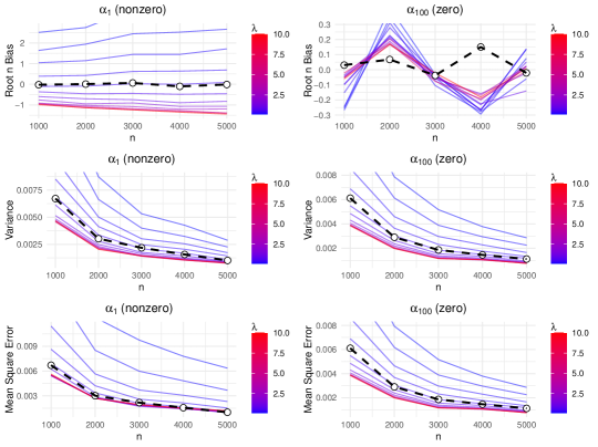
Figure 7: Setting 2 of Section 4.1 (Gaussian design and sparse regression coefficients).

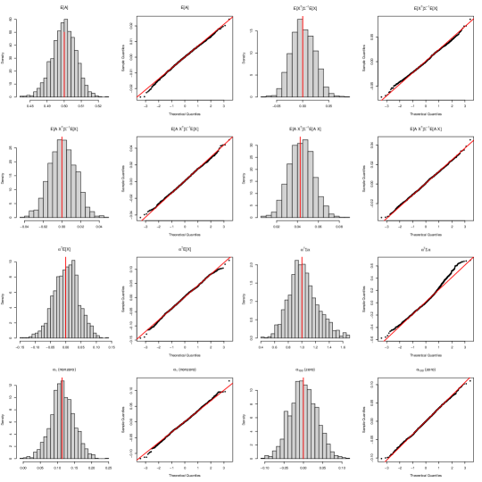
Figure 8: Setting 2 of Section 4.1 (Gaussian design and sparse regression coefficients): Sampling distributions of the moment estimators and the parameter estimators, over 500 Monte Carlos are displayed for the case of $n=5000$.

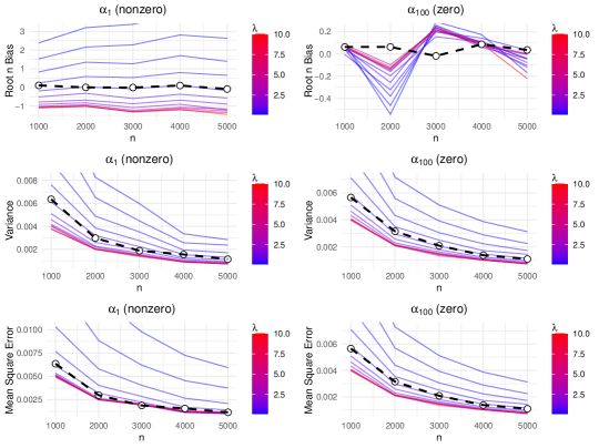
Figure 9: Setting 4 of Section 4.1 (Rademacher design and sparse regression coefficients).

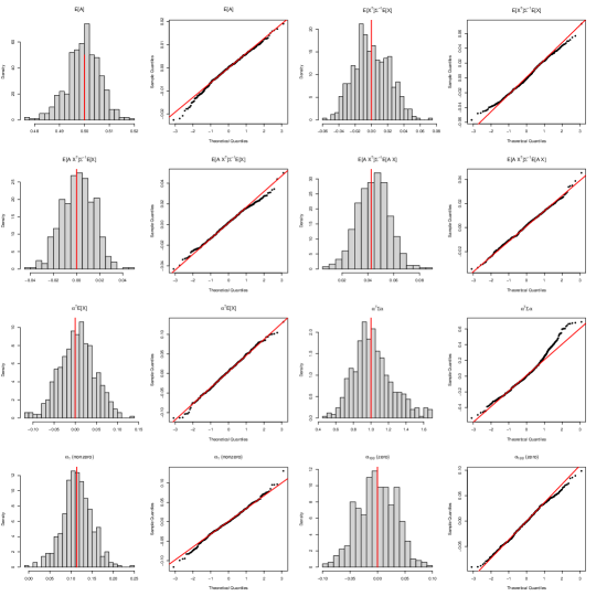
Figure 10: Setting 4 of Section 4.1 (Rademacher design and sparse regression coefficients): Sampling distributions of the moment estimators and the parameter estimators, over 500 Monte Carlos are displayed for the case of $n=5000$.

H.2 A simulation setting where universality does not hold

As we mentioned in Remark 13, the delocalization of regression coefficients or conditions alike shall be necessary to establish universality. Therefore, in this section, we conduct numerical experiments where Assumption $\mathsf{U}$(2) or Assumption $\mathsf{U_{0}}$(2) is violated and demonstrate that the identification strategy based on Gaussian design indeed fails to deliver the correct estimates of the quadratic form or a single coordinate. To this end, we consider the following DGP:

The results are summarized in Figures 11 and 12 below. It is clear that our MoM estimators of the quadratic form $\gamma_{\alpha}^{2}\equiv\bm{\alpha}^{\top}\mathbf{\Sigma}\bm{\alpha}$ and the single coordinate $\alpha_{1}$ are quite different from the true target parameters. For example, speculating Figure 12, the histogram of $\widehat{\alpha}_{1}$ over 500 Monte Carlos does not even cover the true value of $\alpha_{1}$; similarly, the true value of $\gamma_{\alpha}^{2}$ is on the edge of the histogram of $\widehat{\gamma}_{\alpha}^{2}$ over 500 Monte Carlos. Interestingly, when $\lambda$ is relatively large, the debiased estimator of Bellec (2022) has $\sqrt{n}\times\mathrm{bias}$ close to 0. It will be interesting to further investigate the effect of $\lambda$ on the bias, variance, and mean squared error of the de-biased estimators.

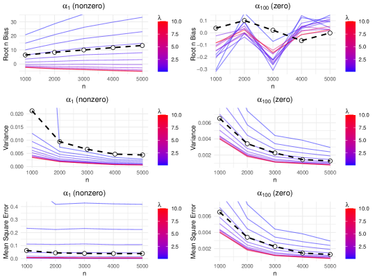
Figure 11: Setting in Appendix H.2.

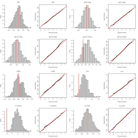
Figure 12: Setting for Appendix H.2: Sampling distributions of the moment estimators and the parameter estimators, over 500 Monte Carlos are displayed for the case of $n=5000$.

H.3 Estimating the mean response under MAR: the non-Gaussian design

In this section, we revisit the numerical experiments in Section 4.2, with the Gaussian design replaced by the Rademacher design. Here we only consider the setting with dense regression coefficients. The results are very similar to the settings with the Gaussian design.

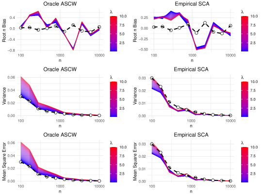
Figure 13: Simulation result for Setting 2 (dense regression coefficients) in Section 4.2, but with the Gaussian design replaced by the Rademacher design. The two methods proposed in Celentano and Wainwright (2023) are plotted separately in two columns of the figure, with color gradients from blue to red representing the increasing value of the tuning parameter $\lambda$. The MoM-based estimators are plotted with white circles and dashed black lines.

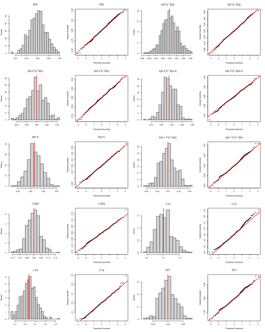
Figure 14: Simulation result for Setting 2 (dense regression coefficients) in Section 4.2, but with the Gaussian design replaced by the Rademacher design. The histograms and normal quantile-quantile plots of of the moment estimators and the estimators of the target parameters, including $\lambda_{\alpha},\gamma_{\alpha}^{2},\gamma_{\alpha,\beta}$ and $\psi$, over 500 Monte Carlos are displayed for the case of $n=5000$.

Finally, the simulation results when the regression coefficients are sparse are reported here in Figures 15 – 16.

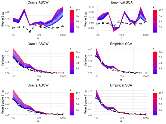
Figure 15: Simulation result for Setting 2 (sparse regression coefficients) in Section 4.2. The two methods proposed in Celentano and Wainwright (2023) are plotted separately in two columns of the figure, with color gradients from blue to red representing the increasing value of the tuning parameter $\lambda$. The MoM-based estimators are plotted with white circles and dashed black lines.

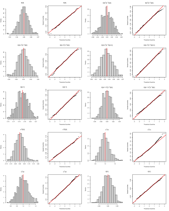
Figure 16: Simulation result for Setting 2 (sparse regression coefficients) in Section 4.2: Sampling distributions of the moment estimators and the parameter estimators, over 500 Monte Carlos are displayed for the case of $n=5000$.

References

• Athey et al. (2018) Susan Athey, Guido W Imbens, and Stefan Wager. Approximate residual balancing: debiased inference of average treatment effects in high dimensions. Journal of the Royal Statistical Society: Series B (Statistical Methodology), 80(4):597–623, 2018.
• Barbier et al. (2019) Jean Barbier, Florent Krzakala, Nicolas Macris, Léo Miolane, and Lenka Zdeborová. Optimal errors and phase transitions in high-dimensional generalized linear models. Proceedings of the National Academy of Sciences, 116(12):5451–5460, 2019.
• Battey and Reid (2023) Heather S Battey and Nancy Reid. On inference in high-dimensional regression. Journal of the Royal Statistical Society Series B: Statistical Methodology, 85(1):149–175, 2023.
• Bayati and Montanari (2011) Mohsen Bayati and Andrea Montanari. The LASSO risk for Gaussian matrices. IEEE Transactions on Information Theory, 58(4):1997–2017, 2011.
• Bayati et al. (2015) Mohsen Bayati, Marc Lelarge, and Andrea Montanari. Universality in polytope phase transitions and message passing algorithms. The Annals of Applied Probability, 25(2):753–822, 2015.
• Bellec (2022) Pierre C Bellec. Observable adjustments in single-index models for regularized ${M}$-estimators. arXiv preprint arXiv:2204.06990, 2022.
• Bellec and Zhang (2022) Pierre C Bellec and Cun-Hui Zhang. De-biasing the lasso with degrees-of-freedom adjustment. Bernoulli, 28(2):713–743, 2022.
• Bellec and Zhang (2023) Pierre C Bellec and Cun-Hui Zhang. Debiasing convex regularized estimators and interval estimation in linear models. The Annals of Statistics, 51(2):391–436, 2023.
• Bhattacharya and Ghosh (1992) Rabi N Bhattacharya and Jayanta K Ghosh. A class of ${U}$-statistics and asymptotic normality of the number of $k$-clusters. Journal of Multivariate Analysis, 43(2):300–330, 1992.
• Bonvini et al. (2024) Matteo Bonvini, Edward H Kennedy, Oliver Dukes, and Sivaraman Balakrishnan. Doubly-robust inference and optimality in structure-agnostic models with smoothness. arXiv preprint arXiv:2405.08525, 2024.
• Bradic et al. (2019a) Jelena Bradic, Victor Chernozhukov, Whitney K Newey, and Yinchu Zhu. Minimax semiparametric learning with approximate sparsity. arXiv preprint arXiv:1912.12213, 2019a.
• Bradic et al. (2019b) Jelena Bradic, Stefan Wager, and Yinchu Zhu. Sparsity double robust inference of average treatment effects. arXiv preprint arXiv:1905.00744, 2019b.
• Cai and Guo (2017) T Tony Cai and Zijian Guo. Confidence intervals for high-dimensional linear regression: Minimax rates and adaptivity. The Annals of Statistics, 45(2):615–646, 2017.
• Cai and Guo (2018) T Tony Cai and Zijian Guo. Accuracy assessment for high-dimensional linear regression. The Annals of Statistics, 46(4):1807–1836, 2018.
• Cai et al. (2023) T Tony Cai, Zijian Guo, and Rong Ma. Statistical inference for high-dimensional generalized linear models with binary outcomes. Journal of the American Statistical Association, 118(542):1319–1332, 2023.
• Candès and Sur (2020) Emmanuel J Candès and Pragya Sur. The phase transition for the existence of the maximum likelihood estimate in high-dimensional logistic regression. The Annals of Statistics, 48(1):27–42, 2020.
• Celentano and Montanari (2024) Michael Celentano and Andrea Montanari. Correlation adjusted debiased lasso: debiasing the lasso with inaccurate covariate model. Journal of the Royal Statistical Society Series B: Statistical Methodology, 2024.
• Celentano and Wainwright (2023) Michael Celentano and Martin J Wainwright. Challenges of the inconsistency regime: Novel debiasing methods for missing data models. arXiv preprint arXiv:2309.01362, 2023.
• Celentano et al. (2023) Michael Celentano, Andrea Montanari, and Yuting Wei. The lasso with general gaussian designs with applications to hypothesis testing. The Annals of Statistics, 51(5):2194–2220, 2023.
• Chatterjee (2006) Sourav Chatterjee. A generalization of the Lindeberg principle. The Annals of Probability, 34(6):2061–2076, 2006.
• Chernozhukov et al. (2018) Victor Chernozhukov, Denis Chetverikov, Mert Demirer, Esther Duflo, Christian Hansen, Whitney Newey, and James Robins. Double/debiased machine learning for treatment and structural parameters. The Econometrics Journal, 21(1):C1–C68, 2018.
• Chernozhukov et al. (2022) Victor Chernozhukov, Juan Carlos Escanciano, Hidehiko Ichimura, Whitney K Newey, and James M Robins. Locally robust semiparametric estimation. Econometrica, 90(4):1501–1535, 2022.
• Christgau et al. (2023) Alexander Mangulad Christgau, Lasse Petersen, and Niels Richard Hansen. Nonparametric conditional local independence testing. The Annals of Statistics, 51(5):2116–2144, 2023.
• Collier et al. (2017) Olivier Collier, Laëtitia Comminges, and Alexandre B Tsybakov. Minimax estimation of linear and quadratic functionals on sparsity classes. The Annals of Statistics, 45(3):923–958, 2017.
• Couillet and Liao (2022) Romain Couillet and Zhenyu Liao. Random Matrix Methods for Machine Learning. Cambridge University Press, 2022.
• Dereziński et al. (2021) Michał Dereziński, Zhenyu Liao, Edgar Dobriban, and Michael W Mahoney. Sparse sketches with small inversion bias. In Conference on Learning Theory, pages 1467–1510. PMLR, 2021.
• Dicker (2014) Lee H Dicker. Variance estimation in high-dimensional linear models. Biometrika, 101(2):269–284, 2014.
• Dudeja et al. (2023a) Rishabh Dudeja, Yue M Lu, and Subhabrata Sen. Universality of approximate message passing with semirandom matrices. The Annals of Probability, 51(5):1616–1683, 2023a.
• Dudeja et al. (2023b) Rishabh Dudeja, Subhabrata Sen, and Yue Lu. Spectral universality of regularized linear regression with nearly deterministic sensing matrices. In Fourteenth International Conference on Sampling Theory and Applications, 2023b.
• Dukes and Vansteelandt (2021) Oliver Dukes and Stijn Vansteelandt. Inference for treatment effect parameters in potentially misspecified high-dimensional models. Biometrika, 108(2):321–334, 2021.
• Gerbelot et al. (2020) Cédric Gerbelot, Alia Abbara, and Florent Krzakala. Asymptotic errors for high-dimensional convex penalized linear regression beyond Gaussian matrices. In Conference on Learning Theory, pages 1682–1713. PMLR, 2020.
• Gerbelot et al. (2022) Cedric Gerbelot, Alia Abbara, and Florent Krzakala. Asymptotic errors for teacher-student convex generalized linear models (or: How to prove Kabashima’s replica formula). IEEE Transactions on Information Theory, 69(3):1824–1852, 2022.
• Guo and Cheng (2022) Xiao Guo and Guang Cheng. Moderate-dimensional inferences on quadratic functionals in ordinary least squares. Journal of the American Statistical Association, 117(540):1931–1950, 2022.
• Guo et al. (2019) Zijian Guo, Wanjie Wang, T Tony Cai, and Hongzhe Li. Optimal estimation of genetic relatedness in high-dimensional linear models. Journal of the American Statistical Association, 114(525):358–369, 2019.
• Han and Shen (2023) Qiyang Han and Yandi Shen. Universality of regularized regression estimators in high dimensions. The Annals of Statistics, 51(4):1799–1823, 2023.
• Hu and Lu (2022) Hong Hu and Yue M Lu. Universality laws for high-dimensional learning with random features. IEEE Transactions on Information Theory, 69(3):1932–1964, 2022.
• Janková and van de Geer (2018) Jana Janková and Sara van de Geer. Semiparametric efficiency bounds for high-dimensional models. The Annals of Statistics, 46(5):2336–2359, 2018.
• Javanmard and Montanari (2014) Adel Javanmard and Andrea Montanari. Confidence intervals and hypothesis testing for high-dimensional regression. Journal of Machine Learning Research, 15(1):2869–2909, 2014.
• Jiang et al. (2022) Kuanhao Jiang, Rajarshi Mukherjee, Subhabrata Sen, and Pragya Sur. A new central limit theorem for the augmented IPW estimator: Variance inflation, cross-fit covariance and beyond. arXiv preprint arXiv:2205.10198, 2022.
• Kakade et al. (2011) Sham M Kakade, Adam Tauman Kalai, Varun Kanade, and Ohad Shamir. Efficient learning of generalized linear and single index models with isotonic regression. In Proceedings of the 24th International Conference on Neural Information Processing Systems, pages 927–935, 2011.
• Kennedy et al. (2024) Edward H Kennedy, Sivaraman Balakrishnan, James M Robins, and Larry Wasserman. Minimax rates for heterogeneous causal effect estimation. The Annals of Statistics, 52(2):793–816, 2024.
• Lahiry and Sur (2023) Samriddha Lahiry and Pragya Sur. Universality in block dependent linear models with applications to nonparametric regression. arXiv preprint arXiv:2401.00344, 2023.
• Lee (2012) John M Lee. Introduction to Smooth Manifolds, volume 218. Springer Science & Business Media, 2012.
• Li and Sur (2023) Yufan Li and Pragya Sur. Spectrum-aware adjustment: A new debiasing framework with applications to principal components regression. arXiv preprint arXiv:2309.07810, 2023.
• Liu and Li (2023) Lin Liu and Chang Li. New $\sqrt{n}$-consistent, numerically stable empirical higher-order influence function estimators. arXiv preprint arXiv:2302.08097, 2023.
• Liu and Wang (2023) Lin Liu and Yuhao Wang. Root-n consistent semiparametric learning with high-dimensional nuisance functions under minimal sparsity. arXiv preprint arXiv:2305.04174, 2023.
• Liu et al. (2017) Lin Liu, Rajarshi Mukherjee, Whitney K Newey, and James M Robins. Semiparametric efficient empirical higher order influence function estimators. arXiv preprint arXiv:1705.07577, 2017.
• Liu et al. (2024) Lin Liu, Rajarshi Mukherjee, and James M Robins. Assumption-lean falsification tests of rate double-robustness of double-machine-learning estimators. Journal of Econometrics, 240(2):105500, 2024.
• McCullagh and Nelder (1989) Peter McCullagh and John A Nelder. Generalized linear models. Routledge, 1989.
• Miolane and Montanari (2021) Léo Miolane and Andrea Montanari. The distribution of the Lasso: Uniform control over sparse balls and adaptive parameter tuning. The Annals of Statistics, 49(4):2313–2335, 2021.
• Montanari and Saeed (2022) Andrea Montanari and Basil N Saeed. Universality of empirical risk minimization. In Conference on Learning Theory, pages 4310–4312. PMLR, 2022.
• Montanari et al. (2023) Andrea Montanari, Feng Ruan, Basil Saeed, and Youngtak Sohn. Universality of max-margin classifiers. arXiv preprint arXiv:2310.00176, 2023.
• Negahban et al. (2012) Sahand N Negahban, Pradeep Ravikumar, Martin J Wainwright, and Bin Yu. A unified framework for high-dimensional analysis of ${M}$-estimators with decomposable regularizers. Statistical Science, 27(4):538–557, 2012.
• Robins et al. (2008) James Robins, Lingling Li, Eric Tchetgen Tchetgen, and Aad van der Vaart. Higher order influence functions and minimax estimation of nonlinear functionals. In Probability and Statistics: Essays in Honor of David A. Freedman, pages 335–421. Institute of Mathematical Statistics, 2008.
• Robins et al. (1994) James M Robins, Andrea Rotnitzky, and Lue Ping Zhao. Estimation of regression coefficients when some regressors are not always observed. Journal of the American Statistical Association, 89(427):846–866, 1994.
• Robins et al. (2023) James M Robins, Lingling Li, Lin Liu, Rajarshi Mukherjee, Eric Tchetgen Tchetgen, and Aad van der Vaart. Minimax estimation of a functional on a structured high-dimensional model (Corrected version). arXiv preprint arXiv:1512.02174, 2023.
• Rotnitzky et al. (2021) Andrea Rotnitzky, Ezequiel Smucler, and James M Robins. Characterization of parameters with a mixed bias property. Biometrika, 108(1):231–238, 2021.
• Sawaya et al. (2023) Kazuma Sawaya, Yoshimasa Uematsu, and Masaaki Imaizumi. Moment-based adjustments of statistical inference in high-dimensional generalized linear models. arXiv preprint arXiv:2305.17731, 2023.
• Scharfstein et al. (1999) Daniel O Scharfstein, Andrea Rotnitzky, and James M Robins. Adjusting for nonignorable drop-out using semiparametric nonresponse models. Journal of the American Statistical Association, 94(448):1096–1120, 1999.
• Shah and Peters (2020) Rajen D Shah and Jonas Peters. The hardness of conditional independence testing and the generalised covariance measure. The Annals of Statistics, 48(3):1514–1538, 2020.
• Smucler et al. (2019) Ezequiel Smucler, Andrea Rotnitzky, and James M Robins. A unifying approach for doubly-robust $\ell_{1}$ regularized estimation of causal contrasts. arXiv preprint arXiv:1904.03737, 2019.
• Song et al. (2024) Yanke Song, Xihong Lin, and Pragya Sur. HEDE: Heritability estimation in high dimensions by Ensembling Debiased Estimators. arXiv preprint arXiv:2406.11184, 2024.
• Stojnic (2013) Mihailo Stojnic. A framework to characterize performance of lasso algorithms. arXiv preprint arXiv:1303.7291, 2013.
• Su et al. (2023) Fangzhou Su, Wenlong Mou, Peng Ding, and Martin Wainwright. When is the estimated propensity score better? High-dimensional analysis and bias correction. arXiv preprint arXiv:2303.17102, 2023.
• Sur (2019) Pragya Sur. A Modern Maximum Likelihood Theory for High-dimensional Logistic Regression. PhD thesis, Stanford University, 2019.
• Sur et al. (2019) Pragya Sur, Yuxin Chen, and Emmanuel J Candès. The likelihood ratio test in high-dimensional logistic regression is asymptotically a rescaled Chi-square. Probability Theory and Related Fields, 175:487–558, 2019.
• Takahashi and Kabashima (2018) Takashi Takahashi and Yoshiyuki Kabashima. A statistical mechanics approach to de-biasing and uncertainty estimation in Lasso for random measurements. Journal of Statistical Mechanics: Theory and Experiment, 2018(7):073405, 2018.
• Tan (2020a) Zhiqiang Tan. Model-assisted inference for treatment effects using regularized calibrated estimation with high-dimensional data. The Annals of Statistics, 48(2):811–837, 2020a.
• Tan (2020b) Zhiqiang Tan. Regularized calibrated estimation of propensity scores with model misspecification and high-dimensional data. Biometrika, 107(1):137–158, 2020b.
• Thrampoulidis et al. (2018) Christos Thrampoulidis, Ehsan Abbasi, and Babak Hassibi. Precise error analysis of regularized ${M}$-estimators in high dimensions. IEEE Transactions on Information Theory, 64(8):5592–5628, 2018.
• van der Laan et al. (2021) Mark van der Laan, Zeyi Wang, and Lars van der Laan. Higher order targeted maximum likelihood estimation. arXiv preprint arXiv:2101.06290, 2021.
• Vansteelandt and Dukes (2022) Stijn Vansteelandt and Oliver Dukes. Assumption-lean inference for generalised linear model parameters. Journal of the Royal Statistical Society Series B: Statistical Methodology, 84(3):657–685, 2022.
• Verzelen and Gassiat (2018) Nicholas Verzelen and Elisabeth Gassiat. Adaptive estimation of high-dimensional signal-to-noise ratios. Bernoulli, 24(4B):3683–3710, 2018.
• Verzelen (2012) Nicolas Verzelen. Minimax risks for sparse regressions: Ultra-high dimensional phenomenons. Electronic Journal of Statistics, 6:38–90, 2012.
• Wang and Shah (2024) Yuhao Wang and Rajen D Shah. Debiased inverse propensity score weighting for estimation of average treatment effects with high-dimensional confounders. The Annals of Statistics, 2024.
• Yadlowsky (2022) Steve Yadlowsky. Explaining practical differences between treatment effect estimators with high dimensional asymptotics. arXiv preprint arXiv:2203.12538, 2022.
• Zhang and Zhang (2014) Cun-Hui Zhang and Stephanie S Zhang. Confidence intervals for low dimensional parameters in high dimensional linear models. Journal of the Royal Statistical Society: Series B (Statistical Methodology), 76(1):217–242, 2014.
• Zhao et al. (2022) Qian Zhao, Pragya Sur, and Emmanuel J Candes. The asymptotic distribution of the MLE in high-dimensional logistic models: Arbitrary covariance. Bernoulli, 28(3):1835–1861, 2022.