Effective and efficient modeling of the hydrodynamics for bacterial flagella

Abstract

The hydrodynamic interactions between bacterial flagella and surrounding boundaries are important for bacterial motility and gait in complex environment. By modeling each flagellar filament that is both thin and long as a string of spheres, we show that such hydrodynamic interactions can be accurately described through a resistance tensor, which can be efficiently evaluated numerically. For the case of close interaction between one bacterium and one passive colloidal sphere, we see notable difference between results from our model and those from the resistive force theory, showing that the error arises from negligence of the width of flagellar filaments in resistive force theory can be strong.

Bacteria are ubiquitous in nature, and a great number of them are motile through the use of flagellar filaments Berg and Turner (1990). Flagellar motility under the influence of the abundant boundary surfaces in environment is not only essential for many biological processes such as fertilization Tung and Suarez (2021); Raveshi et al. (2021), and biofilm formation Nadell et al. (2016), but also important for industrial implications such as the control of the motions of artificial microswimmers Liu et al. (2016). Since for many flagella the length is two to three orders of magnitude larger than the width, accurate capture of their hydrodynamic interactions with close-by boundaries through brute force calculations (e.g., the method of stokeslets Cortez (2001) or boundary element method Ishimoto and Gaffney (2017)) is highly expensive, if feasible. Using Escherichia coli as an example, here we provide a model that enables efficient evaluation of the hydrodynamics of flagella near surfaces with accuracy.

The hydrodynamics of a slender object such as the flagellar filaments are usually evaluated through simplified methods such as the resistive force theory (RFT) Gray and Hancock (1955) or the slender body theory (SBT) Lighthill (1976). By approximations that treats each segment as infinitely thin, these theories are fairly simple and yet still powerful in predicting the total resistance force from fluid. However, the negligence of the width of flagellar filaments makes these theories incapable of evaluation of the hydrodynamic interactions between flagellar segments, and between each segment and other boundary surfaces in environment. To capture these interactions, a model that includes the width of the flagellar filaments is needed. Here we propose a model that treats the flagelar filaments as a string of spheres as illustrated by Fig. 1, where the width of the flagella is characterized by the sphere radius. Since the hydrodynamics between spheres have been well studied and formularized in terms of the resistance matrix Jeffrey and Onishi (1984); Brady and Bossis (1988); Zhang et al. (2021); Leishangthem and Xu (2024), in this study we follow these classical studies and evaluate the hydrodynamics of bacterial flagella.

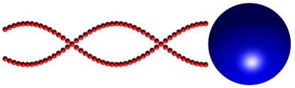
Figure 1: Model of a biflagellate microswimmer. The flagella consist of spheres.

As the characteristic size and speed of E. coli bacteria in water are about $1\mu m$ and $10\mu m/s$, respectively, the corresponding Reynolds number is about $10^{-5}$ so that bacterial flows are typically studied by the linear Stokes equation, which are just:Kim and Karrila (2005); Lauga and Powers (2009):

$$\begin{split}&\mu\nabla^{2}\textbf{u}-\nabla p+\textbf{f}=0,\\ &\nabla\cdot\textbf{u}=0\end{split}$$ (1)

where $\mu$ is the dynamic viscosity, u is the fluid velocity, $p$ is the pressure, and f is the force applied to the fluid by the immersed body. Here, $\rho$, $U$, and $L$ are the fluid density, sphere velocity, and sphere dimension, respectivelyKim and Karrila (2005). Due to the linearity of the Stokes equations, the forces F and torques T that spheres exert on the fluid depend linearly on the translational velocities U and angular velocities $\bm{\Omega}$ of the spheres. On account of the linearity of the Stokes equations, the resistance matrix that relates the forces and torques to the translational and angular velocities of $N$ spheres isDurlofsky et al. (1987); Brady and Bossis (1988); Durlofsky and Brady (1989):

$$\left(\begin{matrix}\textbf{F}\\ \textbf{T}\end{matrix}\right)=\mathcal{R}\left(\begin{matrix}\textbf{U}-\textbf{U}^{\infty}\\ \bm{\Omega}-\bm{\Omega}^{\infty}\end{matrix}\right).$$ (2)

where $\textbf{U}^{\infty}$ and $\bm{\Omega}^{\infty}$ are the ambient flow fields, and $\textbf{U}-\textbf{U}^{\infty}$ and $\bm{\Omega}-\bm{\Omega}^{\infty}$ are vectors of dimension $3N$ of all $N$ spheres relative to the ambient flow. The inverse problem is to calculate the velocities of spheres given their forces and torques:

$$\left(\begin{matrix}\textbf{U}\\ \bm{\Omega}\end{matrix}\right)=\left(\begin{matrix}\textbf{U}^{\infty}\\ \bm{\Omega}^{\infty}\end{matrix}\right)+\mathcal{M}\left(\begin{matrix}\textbf{F}\\ \textbf{T}\end{matrix}\right).$$ (3)

Consider a set of $N$ rigid spheres of arbitrary size immersed in a viscous fluid. Using the twin multipole moment method, the grand resistance matrix $\mathcal{R}$, which contains both near-field lubrication and far-field interactions, can be constructed as

$$\begin{split}\mathcal{R}=(\mathcal{M}^{\infty})^{-1}+\mathcal{R}_{2B,lub}.\end{split}$$ (4)

where the subscript letter ’lub’ indicates ’lubrication’. The grand resistance matrix includes both the far-field interactions via the inversion of $\mathcal{M}^{\infty}$ and the pairwise lubrication interactions $\mathcal{R}_{2B,lub}$. The far-field mobility matrix of multiple spheres, $\mathcal{M}^{\infty}$ is shown as

$$\begin{split}\mathcal{M}^{\infty}=\left(\begin{matrix}\textbf{M}^{tt}_{\alpha\beta}&\textbf{M}^{tr}_{\alpha\beta}\\ \textbf{M}^{rt}_{\alpha\beta}&\textbf{M}^{rr}_{\alpha\beta}\end{matrix}\right).\end{split}$$ (5)

$\mathcal{M}^{\infty}$ is a far-field approximation to the interaction among spheres and includes terms up to $O(s^{-3})$, which is the same as the result of the Rotne-Prager-Yamakawa (RPY) tensor. The detailed elements of $\mathcal{M}^{\infty}$ are given explicitly in Appendix A using the notation of Jeffrey and Onishi (1984). The inverse of $\mathcal{M}^{\infty}$ includes multi-sphere interactions. The pairwise near-field lubrication resistance matrix is denoted as $\mathcal{R}_{2B,lub}$ and constructed as

$$\begin{split}\mathcal{R}_{2B,lub}=\left(\begin{matrix}\textbf{R}^{tt}_{\alpha\beta}&\textbf{R}^{tr}_{\alpha\beta}\\ \textbf{R}^{rt}_{\alpha\beta}&\textbf{R}^{rr}_{\alpha\beta}\end{matrix}\right).\end{split}$$ (6)

for $\xi\leq\min\{\lambda,1/\lambda\}$ and is a zero matrix for $\xi>\min\{\lambda,1/\lambda\}$. The segmentation point for near- and far-field can be smaller than $\min\{\lambda,1/\lambda\}$. $\mathcal{R}_{2B,lub}$ is a continuous function of variable $s$ and is equal to zero when $s=2+\min\{\lambda,1/\lambda\}$ to ensure the continuity of the matrix. This procedure captures both near- and far-field interactions and saves computational costs.

We follow the notation of Jeffrey and Onishi and define the variables $s=2r/(a_{\alpha}+a_{\beta})$, $\xi=s-2$, and $\lambda=a_{\beta}/a_{\alpha}$ (the subscripts $\alpha$ and $\beta$ indicate the labels of the spheres, which take on all values from $1$ to $N$), where $r$ is the center-to-center distance of the inter-sphere and $a_{\alpha}$ is the radius of sphere $\alpha$. Then $\textbf{e}_{\alpha\beta}=\left(\textbf{x}_{\alpha}-\textbf{x}_{\beta}\right)/\left|\textbf{x}_{\alpha}-\textbf{x}_{\beta}\right|$ is the unit vector along the line of centers. The submatrices $\textbf{R}^{tt}_{\alpha\beta}$, $\textbf{R}^{tr}_{\beta\alpha}$, $\textbf{R}^{rt}_{\alpha\beta}$, $\textbf{R}^{rr}_{\alpha\beta}$, $\textbf{M}^{tt}_{\alpha\beta}$, $\textbf{M}^{tr}_{\alpha\beta}$, $\textbf{M}^{rt}_{\alpha\beta}$, and $\textbf{M}^{rr}_{\alpha\beta}$ are second-rank tensors. We define the non-dimensional quantities

$$\begin{split}&\widehat{\textbf{R}}_{\alpha\beta}^{tt}=\frac{\textbf{R}_{\alpha\beta}^{tt}}{3\pi\mu(a_{\alpha}+a_{\beta})},\\ &\widehat{\textbf{R}}_{\alpha\beta}^{rt}=\frac{\textbf{R}_{\alpha\beta}^{rt}}{\pi\mu(a_{\alpha}+a_{\beta})^{2}},\\ &\widehat{\textbf{R}}_{\alpha\beta}^{rr}=\frac{\textbf{R}_{\alpha\beta}^{rr}}{\pi\mu(a_{\alpha}+a_{\beta})^{3}},\\ &\widehat{\textbf{M}}_{\alpha\beta}^{tt}=3\pi\mu(a_{\alpha}+a_{\beta})\textbf{M}_{\alpha\beta}^{tt},\\ &\widehat{\textbf{M}}_{\alpha\beta}^{rt}=\pi\mu(a_{\alpha}+a_{\beta})^{2}\textbf{M}_{\alpha\beta}^{rt},\\ &\widehat{\textbf{M}}_{\alpha\beta}^{rr}=\pi\mu(a_{\alpha}+a_{\beta})^{3}\textbf{R}_{\alpha\beta}^{rr}.\end{split}$$ (7)

Then the non-dimensional submatrices can be expressed as follows, respectively

$$\begin{split}&\widehat{\textbf{R}}_{\alpha\beta}^{tt}=X_{\alpha\beta}^{a}\textbf{e}_{\alpha\beta}\otimes\textbf{e}_{\alpha\beta}+Y_{\alpha\beta}^{a}(\mathbb{I}-\textbf{e}_{\alpha\beta}\otimes\textbf{e}_{\alpha\beta}),\\ &\widehat{\textbf{R}}_{\alpha\beta}^{rt}=\left[\widehat{\textbf{R}}_{\beta\alpha}^{tr}\right]^{T}=Y_{\alpha\beta}^{b}(\textbf{e}_{\alpha\beta}\times),\\ &\widehat{\textbf{R}}_{\alpha\beta}^{rr}=X_{\alpha\beta}^{c}\textbf{e}_{\alpha\beta}\otimes\textbf{e}_{\alpha\beta}+Y_{\alpha\beta}^{c}(\mathbb{I}-\textbf{e}_{\alpha\beta}\otimes\textbf{e}_{\alpha\beta}).\end{split}$$ (8)

and

$$\begin{split}&\widehat{\textbf{M}}_{\alpha\beta}^{tt}=x_{\alpha\beta}^{a}\textbf{e}_{\alpha\beta}\otimes\textbf{e}_{\alpha\beta}+y_{\alpha\beta}^{a}(\mathbb{I}-\textbf{e}_{\alpha\beta}\otimes\textbf{e}_{\alpha\beta}),\\ &\widehat{\textbf{M}}_{\alpha\beta}^{rt}=\left[\widehat{\textbf{M}}_{\beta\alpha}^{tr}\right]^{T}=y_{\alpha\beta}^{b}(\textbf{e}_{\alpha\beta}\times),\\ &\widehat{\textbf{M}}_{\alpha\beta}^{rr}=x_{\alpha\beta}^{c}\textbf{e}_{\alpha\beta}\otimes\textbf{e}_{\alpha\beta}+y_{\alpha\beta}^{c}(\mathbb{I}-\textbf{e}_{\alpha\beta}\otimes\textbf{e}_{\alpha\beta}).\end{split}$$ (9)

where $\mathbb{I}$ is a $3\times 3$ identity matrix, $\otimes$ is the dyadic product, and $(\textbf{e}\times)$ is a $3\times 3$ antisymmetric matrix defined by $(\textbf{e}\times)\textbf{v}=\textbf{e}\times\textbf{v}$ for any v. The elements of the matrix obey a number of symmetry conditions, which are given in Jeffrey and Onishi Jeffrey and Onishi (1984). The specific expressions of resistance and mobility functions are provided in Appendix A. The grand resistance matrix $\mathcal{R}$ written in terms of individual elements is

$$\begin{split}\mathcal{R}=\left(\begin{matrix}\mathcal{R}^{tt}_{\alpha\beta}&\mathcal{R}^{tr}_{\alpha\beta}\\ \mathcal{R}^{rt}_{\alpha\beta}&\mathcal{R}^{rr}_{\alpha\beta}\end{matrix}\right).\end{split}$$ (10)

where the non-dimensional submatrices of $\widehat{\mathcal{R}}$ are expressed as:

$$\begin{split}&\widehat{\mathcal{R}}_{\alpha\beta}^{tt}=X_{\alpha\beta}^{A}\textbf{e}_{\alpha\beta}\otimes\textbf{e}_{\alpha\beta}+Y_{\alpha\beta}^{A}(\mathbb{I}-\textbf{e}_{\alpha\beta}\otimes\textbf{e}_{\alpha\beta}),\\ &\widehat{\mathcal{R}}_{\alpha\beta}^{rt}=\left[\widehat{\mathcal{R}}_{\beta\alpha}^{tr}\right]^{T}=Y_{\alpha\beta}^{B}(\textbf{e}_{\alpha\beta}\times),\\ &\widehat{\mathcal{R}}_{\alpha\beta}^{rr}=X_{\alpha\beta}^{C}\textbf{e}_{\alpha\beta}\otimes\textbf{e}_{\alpha\beta}+Y_{\alpha\beta}^{C}(\mathbb{I}-\textbf{e}_{\alpha\beta}\otimes\textbf{e}_{\alpha\beta}).\end{split}$$ (11)

The scalar grand resistance functions $X^{A}$, $Y^{A}$, $Y^{B}$, $X^{C}$, and $Y^{C}$ are plotted versus the reduced inter-sphere separation distance, $s=2r/(a_{\alpha}+a_{\beta})$, in Fig. 2-6, respectively. The grand mobility matrix is the inverse of the grand resistance matrix

$$\begin{split}\mathcal{M}=\mathcal{R}^{-1}.\end{split}$$ (12)

The grand mobility matrix $\mathcal{M}$ obtained by this method is convergent at any reduced separation distance $s$. For near-field lubrication, the term $\xi^{-1}$ is introduced in longitudinal resistance functions $X^{A}$ to avoid overlapping spheres in numerical simulation. We examine the results for the resistance functions and compare them, where available, with those obtained by the RPY tensor. Several resistance functions of two equal spheres are plotted as functions of the reduced separation distance $s$ in Fig. 2-6, respectively. These plots were generated by the variable $s$ in the region $2.0\leq s\leq 6.0$.

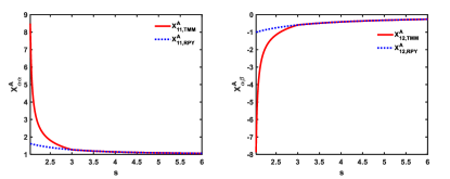
Figure 2: Longitudinal resistance functions coupling the longitudinal force of one sphere to the longitudinal translational velocity of that and other spheres. Comparison of the twin multipole moment method (TMM) and the Rotne-Prager-Yamakawa (RPY) tensor for scalar resistance functions $X_{\alpha\alpha}^{A}$ and $X_{\alpha\beta}^{A}$ as a function of $s$.

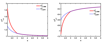
Figure 3: Transverse resistance functions coupling the transverse force of one sphere to the transverse translational velocity of that and other spheres. Comparison of the twin multipole moment method (TMM) and the Rotne-Prager-Yamakawa (RPY) tensor for scalar resistance functions $Y_{\alpha\alpha}^{A}$ and $Y_{\alpha\beta}^{A}$ as a function of $s$.

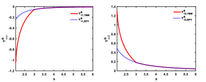
Figure 4: Coupling of torque and rotation. The resistance functions $Y_{\alpha\alpha}^{B}$ and $Y_{\alpha\beta}^{B}$ coupling the torque of one sphere to its own and others’ rotation. Comparison of the twin multipole moment method (TMM) and the Rotne-Prager-Yamakawa (RPY) tensor for scalar resistance functions $Y_{\alpha\alpha}^{B}$ and $Y_{\alpha\beta}^{B}$ as a function of $s$.

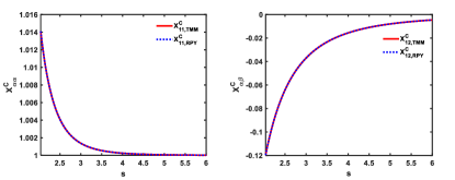
Figure 5: Longitudinal resistance functions coupling the longitudinal torque of a sphere to the longitudinal rotational velocity of that and other spheres. Comparison of the twin multipole moment method (TMM) and the Rotne-Prager-Yamakawa (RPY) tensor for scalar resistance functions $X_{\alpha\alpha}^{C}$ and $X_{\alpha\beta}^{C}$ as a function of $s$.

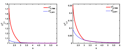
Figure 6: Transverse resistance functions coupling the transverse torque of a sphere to the transverse rotational velocity of that and other spheres. Comparison of the twin multipole moment method (TMM) and the Rotne-Prager-Yamakawa (RPY) tensor for scalar resistance functions $Y_{\alpha\alpha}^{C}$ and $Y_{\alpha\beta}^{C}$ as a function of $s$.

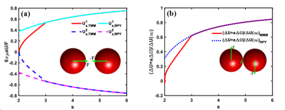
Figure 7: (a) The translational velocities of two equal spheres dragged by force F and $-\textbf{F}$ along the $x$-axis versus the reduced separation distance $s$. (b) The velocity difference of two equal spheres dragged by force F and $-\textbf{F}$ along the $y$-axis versus the reduced separation distance $s$. The results are obtained by the twin multipole moment method (TMM) and the Rotne-Prager-Yamakawa (RPY) tensor, respectively.

The longitudinal components $X^{A}$ of the resistance matrix $\mathcal{R}^{tt}$ are plotted in Fig. 2, which couple the longitudinal force and the longitudinal translational velocity. When the spheres come into contact with each other, that is, $s=2$, the scalar resistance functions $X^{A}$ tend to infinity, which automatically avoids the overlapping of two spheres. These components include near-field lubrication, which is significantly different from the components of the RPY tensor. Physically, a sphere can move freely when the other spheres are far away, then the self-mobility components $X^{A}_{\alpha\alpha}\to 1$ and the pair mobility components $X^{A}_{\alpha\beta}\to 0$. The transverse components $Y^{A}$ of the resistance matrix $\mathcal{R}^{tt}$ are plotted in Fig. 3, which couple the transverse force and the transverse translational velocity. The self-mobility components $Y^{A}_{\alpha\alpha}\to 1$ and the pair mobility components $Y^{A}_{\alpha\beta}\to 0$ when a pair of spheres are widely separated.

The resistance functions $Y^{B}$ in Fig. 4 give the coupling between the force and rotational velocity or torque and translational velocity. When a pair of spheres is widely separated, a hydrodynamic force or torque on one will induce no rotation or translation of the other. This means that the components $Y^{B}_{\alpha\alpha}\to 0$ and $Y^{B}_{\alpha\beta}\to 0$ when $s\to\infty$. As a sphere approaches another sphere, the drag force or torque on one sphere will induce rotation or translation of the other.

The longitudinal components $X^{C}$ of the resistance matrix $\mathcal{R}^{rr}$ are plotted in Fig. 5, which couple the longitudinal torque and the longitudinal rotational velocity. Fig. 5 shows that the resistance functions $X^{C}$ obtained by the twin multipole moment method (TMM) and the Rotne-Prager-Yamakawa (RPY) tensor are the same. The self-mobility components $X^{C}_{\alpha\alpha}\to 1$ and the pair mobility components $X^{C}_{\alpha\beta}\to 0$ when a pair of spheres is far away from each other. The transverse components $Y^{C}$ of the resistance matrix $\mathcal{R}^{rr}$ are plotted in Fig. 6, which give the coupling between the torque and rotational velocity perpendicular to the line of centers.

As an example, in Fig. 7(a), we compare the translational velocities of two equal spheres dragged by forces F and $-\textbf{F}$ computed by the grand resistance matrix and RPY tensor, respectively. Rather than moving very slowly toward one another, two spheres would physically touch and overlap if there were no other repulsive forces present to prevent contact. Using the grand resistance matrix, we find that the translational velocity gradually tends to $0$ as $s$ approaches $2.0$, which is very different from the result obtained by the RPY tensor. The grand resistance matrix constructed here automatically prevents the overlapping of spheres, enabling us not to need to introduce repulsive potential Schroeder et al. (2004); Loi et al. (2011); Jendrejack et al. (2003, 2004); Ando and Skolnick (2013); Schlick and Olson (1992).

The prediction of the no-slip boundary condition is $\left[(U_{y}^{1}-U_{y}^{2})+a(\Omega_{z}^{1}+\Omega_{z}^{2})\right]/\left(U_{y}^{1}(\infty)-U_{y}^{2}(\infty)\right)=0$ at $s=2$, where $U_{y}^{1}(\infty)=F/6\pi\mu a$ and $U_{y}^{2}(\infty)=-F/6\pi\mu a$, where U and $\bm{\Omega}$ are the translational and rotational velocities of the centers of the spheres, respectively. In order to demonstrate that the grand resistance matrix satisfies the no-slip boundary condition, two equal spheres are lined along the $x$-axis, and then the forces F and $-\textbf{F}$ are applied to the two spheres along the $y$-axis, respectively. The numerical simulation is found to match our prediction at mall separation distance $s\to 2$, as shown in Fig. 7(b). This means that the no-slip boundary condition has been approximately achieved at the point ’A’ of closest approach, and the transverse translation vanishes, but rotation is still possible. The reason why the result slightly deviates from $0$ when $s\to 2$ is that we neglect the higher-order terms when calculating the matrix $\mathcal{R}$. These higher-order terms will increase the computational cost but have little impact on the results. The result calculated by the Rotne-Prager-Yamakawa (RPY) tensor is significantly different from our prediction.

In order to verify the accuracy of the bead-rod model and determine the appropriate bead spacing, the propulsion of a helical rigid flagellum is simulated and compared with Rodenborn’s workRodenborn et al. (2013). A helical flagellum can be modeled as a rigid rotating helix with radius $R$, pitch $\lambda$, axial length $L$, pitch angle $\theta$, filament radius $a$, contour length $\Lambda=L/\cos\theta$, and wave number $k=2\pi/\lambda$, where $\tan\theta=2\pi R/\lambda$. We consider a rigid bacterial flagellum as a string of spheres embedded in a viscous fluid and represent it as a helical sequence of $N$ spheres, as shown in Fig. 8. The centerline of the left-handed helical flagellum is given as follows:

$$\begin{split}\textbf{r}(s)=[x,\sin(kx+\Omega t),\cos(kx+\Omega t)],\quad x\in[0,L].\end{split}$$ (13)

where $x=s\cos\theta$, $\Omega$ is the rotation rate, and $k$ is the helix wave number. The helical flagellum is divided into $N$ equidistant discrete spheres with radius $a$, then, the translational velocity U and rotational velocity $\bm{\Omega}$ related to the forces F and torques T exerted on the fluid are

$$\left(\begin{matrix}\textbf{F}\\ \textbf{T}\end{matrix}\right)=\mathcal{R}\left(\begin{matrix}\textbf{U}\\ \bm{\Omega}\end{matrix}\right).$$ (14)

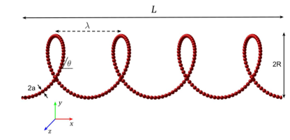
Figure 8: Schematic of a helical flagellum model. The helix radius of the flagellum is $R$, helix pitch is $\lambda$, axial length is $L$, filament radius is $a$, contour length is $\Lambda=L/\cos\theta$, and the pitch angle is $\theta$, where $\tan\theta=2\pi R/\lambda$. The inset shows the direction of the coordinate system.

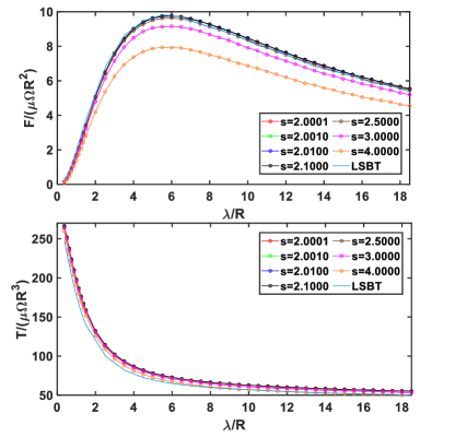
Figure 9: Dimensionless thrust and torque for a helical flagellum as a function of pitch $\lambda$ for helix length $L=20R$ and filament radius $a=R/16$ for various values of $s$, and compared with the results of Lighthill slender body theory (cyan solid line).

Axial thrust $F$ and torque $T$ for a rotating, non-translating flagellum can be calculated from the above equation. The helix radius $R$ is used as the unit of length; thrust and torque are made dimensionless by dividing by $\mu\Omega R^{2}$ and $\mu\Omega R^{2}$. Our results computed for the thrust $F$ and torque $T$ for a helical flagellum with radius $a=R/16$ are shown in Fig. 9 as a function of the helix pitch $\lambda$; the axial length is $L=20R$. The total axial thrust $F=\sum_{i=1}^{N}\textbf{f}_{i}\cdot\textbf{e}_{x}$ and torque $T=\sum_{i=1}^{N}[\textbf{n}_{i}+(\textbf{r}_{i}-\textbf{r}_{1})\times\textbf{f}_{i}]\cdot\textbf{e}_{x}$, where $\textbf{f}_{i}$ and $\textbf{n}_{i}$ are the force and torque applied to the sphere $i$ by the fluid, respectively. The cyan solid line is obtained using Lighthill slender body theory (LSBT) Lighthill (1976), and the circle solid lines are obtained using the twin multipole moment method for various $s$. The results obtained by Lighthill slender body theory and twin multipole moment method in the interval of $2.0001\leq s\leq 2.5000$ are consistent.

The flagella are slender, and their filament radius $a$ is much smaller than other geometric parameters. Resistive force theory Gray and Hancock (1955); Chwang and Wu (1975); Lighthill (1976), slender body theoryLighthill (1976), regularized Stokeslet method Cortez (2001); Cortez et al. (2005), boundary element method Smith et al. (2009), and immersed boundary method Lim et al. (2008) are often used for numerical simulations. Our results agree with Rodenborn’s laboratory measurement and the numerical simulations conducted using the Lighthill slender body theory and regularized Stokeslet method. However, The resistive force theory and slender body theory are only suitable for slender bodies. The calculating costs of the regularized Stokeslet method, boundary element method, and immersed boundary method are expensive. One usually models the cell body of a microswimmer as a sphere Riley et al. (2018); Dvoriashyna and Lauga (2021), slender body theory cannot include the hydrodynamic interactions between the cell body and the flagella, which require other methods to calculate, such as the method of image Higdon (1979); Huang and Jawed (2020). However, the twin multipole moment method treats the flagella and cell bodies of microswimmers as spheres, simplifying the microswimmer model.

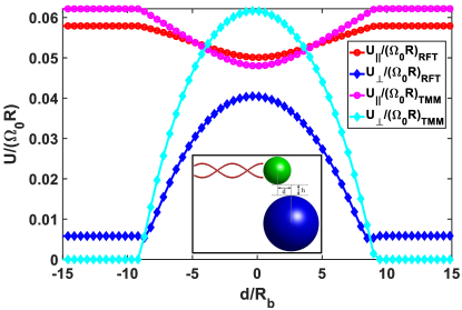
Figure 10: Comparisons between the resistive force theory (RFT) and twin multipole moment method (TMM) in terms of the forward swimming speed ($\parallel$) and transverse speed ($\perp$). The inset shows the model of a biflagellate microswimmer near a spherical obstacle.

Fig. 10 compares the simulation results obtained by the resistive force theory (RFT) and the twin multipole moment method (TMM) of a biflagellate microswimmer near a spherical obstacle. The microswimmer consists of two helical flagellum and a spherical cell body. The radius of cell body is $R_{b}$, helix radius is $R=R_{b}/2$, filament radius $a=R_{b}/16$, pitch angle $\theta=\pi/5$, contour length of flagella is $\Lambda=10R_{b}$, and the radius of the spherical obstacle is $R_{s}=100R_{b}$. Resistive force theory is only used to calculate the propulsive force of the flagella, neglect the hydrodynamic interactions between flagella and cell body and obstacle, and the the hydrodynamic interaction between cell body and obstacle is also calculated using the twin multipole moment method. The twin multipole moment method treats the flagella as a string of spheres, and consider all hydrodynamic interactions between the cell body, flagella, and obstacle. We compare the forward swimming speed ($\parallel$) and transverse speed ($\perp$), the longitudinal distance between the cell body and obstacle center $d$, the transverse distance between the cell body and obstacle center $h$. Fig. 10 shows that the hydrodynamic interaction between cell body and obstacle, flagella and obstacle significantly affect the forward swimming speed and transverse speed.

The commonly used methods for solving linear equations include the inverse matrix method (IMM) and the generalized minimal residual method (GMRES). In this section, we test the computing time required to solve Eq. 2. Herein, the dimension of the resistance matrix is $6N\times 6N$. The motion equation $\left[(\mathcal{M}^{\infty})^{-1}+\mathcal{R}_{2B,lub}\right]\cdot\textbf{U}=\textbf{F}$ is equivalent to $\left(\mathbb{I}+\mathcal{M}^{\infty}\cdot\mathcal{R}_{2B,lub}\right)\cdot\textbf{U}=\mathcal{M}^{\infty}\cdot\textbf{F}$, which saves calculating cost. We take a rigid helical flagellum and three-dimensional randomly distributed spheres as examples. For both spheres and flagellum, we record data from $40$ independent runs for each $\{N,Time\}$. These simulations were performed on laptop-$1$ (Intel i7-10750H, $2933$ MHz CPU clock speed, and $40$ GB RAM) and laptop-$2$ (Intel i7-12700H, $4800$ MHz CPU clock speed, and $64$ GB RAM), respectively.

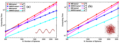
Figure 11: Computing Time of the motion equation varies with the number of spheres using the inverse matrix method (IMM) and the generalized minimal residual method (GMRES), respectively. (a) Simulation of a helical flagellum using two different laptops with two different methods. Inset shows a helical flagellum. (b) Simulation of 3D randomly distributed spheres using two different laptops with two different methods. Inset shows 3D randomly distributed spheres.

The computing time of the motion equation $\left(\mathbb{I}+\mathcal{M}^{\infty}\cdot\mathcal{R}_{2B,lub}\right)\cdot\textbf{U}=\mathcal{M}^{\infty}\cdot\textbf{F}$ for two different models is shown in Fig. 11. The computing time using the inverse matrix method is asymptotically proportional to $\sim N^{3}$. However, the computing time using generalized minimal residual method is asymptotically proportional to $\sim N^{2}$. The cost of calculating the motion equation with the generalized minimal residual method is much lower than with the inverse matrix method.

We propose a technique to construct the resistance and mobility matrix that takes account of both the near-field lubrication and far-field hydrodynamic interactions of a set of rigid spheres of arbitrary size immersed in a viscous fluid. The far-field mobility matrix $\mathcal{M}^{\infty}$ only considers long-range hydrodynamic interactions, and the formulation is exactly the same as the Rotne-Prager-Yamakawa tensor. We first invert $\mathcal{M}^{\infty}$ to obtain a far-field approximation to the grand resistance matrix $\mathcal{R}$. However, this multi-sphere approximation to the grand resistance matrix still lacks lubrication. To include near-field lubrication, we introduce it in a pairwise additive fashion $\mathcal{R}_{2B,lub}$ in the grand resistance matrix. However, the lubrication is only available for $\xi\leq\min\{\lambda,1/\lambda\}$. Thus, our approach to the grand resistance matrix $\mathcal{R}$, which contains both near-field lubrication and far-field multi-sphere interactions, is $\mathcal{R}=(\mathcal{M}^{\infty})^{-1}+\mathcal{R}_{2B,lub}$. Once the grand resistance matrix $\mathcal{R}$ is obtained, the grand mobility matrix can be obtained by inverting it, $\mathcal{M}=(\mathcal{R})^{-1}$.

We consider a rotating, non-translating helical rigid flagellum, which is divided into a set of $N$ identical, uniformly spaced spheres. Our calculations of axial thrust and torque for the flagellum with different pitches are presented in Fig. 9. The grand resistance matrix constructed here captures both near- and far-field interactions. To illustrate the effect of the inter-sphere separation distance, models with different $s$ values are calculated. Which gives excellent results in the region $2.0001\leq s\leq 2.5000$ compared with Rodenborn’s laboratory measurements Rodenborn et al. (2013). This conclusion indicates that the selection of $s$ for the rigid filament model between interval $2.0\leq s\leq 2.5$ has little effect on the calculation results.

Our technique for calculating the grand resistance matrix is suitable for investigating the hydrodynamic interaction between multi-sphere systems, such as bacterial systems. This technique for constructing the grand resistance matrix has three main merits: it avoids overlapping spheres, approximately satisfies the no-slip boundary condition, and includes all long-range terms. Our method can be easily extended to compute the grand resistance or mobility matrix for arbitrary-size spheres. While this method is accurate and efficient, it is still computationally expensive. The construction of a near-field lubrication resistance matrix requires $O(N^{2})$ operations. The hydrodynamic interaction between multiple spheres is obtained by inverting the mobility matrix in the grand resistance matrix, which requires $O(N^{3})$ operations and limits the size of systems that can be studied. This method does not consider the flow field around the spheres, and we will present a method in our next work to investigate the flow field around spheres.

We acknowledge computational support from Beijing Computational Science Research Center. This work is supported by the National Natural Science Foundation of China (NSFC) No. U2230402, and China Postdoctoral Science Foundation No. 2022M712927.

Appendix A. The scalar resistance and mobility functions

We follow the notation of Jeffrey and Onishi, define the variables $s=2r/(a_{\alpha}+a_{\beta})$, $\xi=s-2$ and $\lambda=a_{\beta}/a_{\alpha}$ (the subscripts $\alpha$, and $\beta$ indicate the labels for the spheres, which take on all values from $1$ to $N$), where $r$ is the center-to-center distance of the inter-sphere and $a_{\alpha}$ is the radius of the sphere $\alpha$. The scalar resistance functions for $\xi\leq\min\{\lambda,1/\lambda\}$ are:

1. The scalar resistance functions $X^{a}$

$$\begin{split}&X_{\alpha\alpha}^{a}=g_{1}(\lambda)\xi^{-1},\\ &X_{\alpha\beta}^{a}=-\frac{2}{1+\lambda}\left[g_{1}(\lambda)\xi^{-1}\right].\end{split}$$ (15)

where

$$\begin{split}g_{1}(\lambda)=2\lambda^{2}(1+\lambda)^{-3}.\end{split}$$ (16)

2. The scalar resistance functions $Y^{a}$

$$\begin{split}&Y_{\alpha\alpha}^{a}=g_{2}(\lambda)\ln(\xi^{-1}),\\ &Y_{\alpha\beta}^{a}=-\frac{2}{1+\lambda}\left[g_{2}(\lambda)\ln(\xi^{-1})\right].\end{split}$$ (17)

where

$$\begin{split}g_{2}(\lambda)=\frac{4}{15}\lambda(2+\lambda+2\lambda^{2})(1+\lambda)^{-3}.\end{split}$$ (18)

3. The scalar resistance functions $Y^{b}$

$$\begin{split}&Y_{\alpha\alpha}^{b}=g_{2}(\lambda)\ln(\xi^{-1}),\\ &Y_{\alpha\beta}^{b}=-\frac{4}{(1+\lambda)^{2}}\left[g_{2}(\lambda)\ln(\xi^{-1})\right].\end{split}$$ (19)

where

$$\begin{split}g_{2}(\lambda)=-\frac{1}{5}\lambda(4+\lambda)(1+\lambda)^{-2}.\end{split}$$ (20)

4. The scalar resistance functions $X^{c}$

$$\begin{split}&X_{\alpha\alpha}^{c}=1,\\ &X_{\alpha\beta}^{c}=0.\end{split}$$ (21)

5. The scalar resistance functions $Y^{c}$

$$\begin{split}&Y_{\alpha\alpha}^{c}=g_{2}(\lambda)\ln(\xi^{-1}),\\ &Y_{\alpha\beta}^{c}=g_{4}(\lambda)\ln(\xi^{-1}).\end{split}$$ (22)

where

$$\begin{split}g_{2}(\lambda)=\frac{2}{5}\lambda(1+\lambda)^{-1},\quad g_{4}(\lambda)=\frac{4}{5}\lambda^{2}(1+\lambda)^{-4}.\end{split}$$ (23)

The scalar mobility functions are:

$$\begin{split}&x_{\alpha\alpha}^{a}=1,\qquad x_{\alpha\beta}^{a}=3/2s^{-1}-(2+2\lambda^{2})/(1+\lambda)^{2}s^{-3},\\ &y_{\alpha\alpha}^{a}=1,\qquad y_{\alpha\beta}^{a}=3/4s^{-1}+(1+\lambda^{2})/(1+\lambda)^{2}s^{-3},\\ &y_{\alpha\alpha}^{b}=0,\qquad y_{\alpha\beta}^{b}=-1/2s^{-2},\\ &x_{\alpha\alpha}^{c}=1,\qquad x_{\alpha\beta}^{c}=s^{-3},\\ &y_{\alpha\alpha}^{c}=1,\qquad y_{\alpha\beta}^{c}=-1/2s^{-3}.\end{split}$$ (24)

The sphere labels $\alpha$ and $\beta$ can be interchanged.

References

- Berg and Turner (1990) H. C. Berg and L. Turner, Biophysical Journal 58, 919 (1990).
- Tung and Suarez (2021) C. K. Tung and S. S. Suarez, Cells 10, 1297 (2021).
- Raveshi et al. (2021) M. R. Raveshi, M. S. A. Halim, S. N. Agnihotri, M. K. O’Bryan, A. Neild, and R. Nosrati, Nature Communications 12, 3446 (2021).
- Nadell et al. (2016) C. D. Nadell, K. Drescher, and K. R. Foster, Nature Reviews Microbiology 14, 589 (2016).
- Liu et al. (2016) C. Liu, C. Zhou, W. Wang, and H. P. Zhang, Phys. Rev. Lett. 117, 198001 (2016).
- Cortez (2001) R. Cortez, SIAM J. Sci. Comput. 23, 1204 (2001).
- Ishimoto and Gaffney (2017) K. Ishimoto and E. A. Gaffney, J. Fluid Mech. 831, 228 (2017).
- Gray and Hancock (1955) J. Gray and G. J. Hancock, Journal of Experimental Biology 32, 802 (1955).
- Lighthill (1976) J. Lighthill, SIAM review 18, 161 (1976).
- Jeffrey and Onishi (1984) D. J. Jeffrey and Y. Onishi, J. Fluid Mech. 139, 261 (1984).
- Brady and Bossis (1988) J. F. Brady and G. Bossis, Annu. Rev. Fluid Mech. 20, 111 (1988).
- Zhang et al. (2021) B. K. Zhang, P. Leishangthem, Y. Ding, and X. L. Xu, Proc. Natl. Acad. Sci. U.S.A. 118, e2100145118 (2021).
- Leishangthem and Xu (2024) P. Leishangthem and X. L. Xu, Phys. Rev. Lett. 132, 238302 (2024).
- Kim and Karrila (2005) S. Kim and S. J. Karrila, Microhydrodynamics: principles and selected applications (Courier Corporation, 2005).
- Lauga and Powers (2009) E. Lauga and T. R. Powers, Reports on progress in physics 72, 096601 (2009).
- Durlofsky et al. (1987) L. Durlofsky, J. F. Brady, and G. Bossis, Journal of fluid mechanics 180, 21 (1987).
- Durlofsky and Brady (1989) L. J. Durlofsky and J. F. Brady, Journal of Fluid Mechanics 200, 39 (1989).
- Schroeder et al. (2004) C. M. Schroeder, E. S. G. Shaqfeh, and S. Chu, Macromolecules 37, 9242 (2004).
- Loi et al. (2011) D. Loi, S. Mossa, and L. F. Cugliandolo, Soft Matter 7, 10193 (2011).
- Jendrejack et al. (2003) R. M. Jendrejack, D. C. Schwartz, M. D. Graham, and J. J. De Pablo, The Journal of chemical physics 119, 1165 (2003).
- Jendrejack et al. (2004) R. M. Jendrejack, D. C. Schwartz, J. J. De Pablo, and M. D. Graham, The Journal of chemical physics 120, 2513 (2004).
- Ando and Skolnick (2013) T. Ando and J. Skolnick, Biophysical journal 104, 96 (2013).
- Schlick and Olson (1992) T. Schlick and W. K. Olson, Science 257, 1110 (1992).
- Rodenborn et al. (2013) B. Rodenborn, C. H. Chen, H. L. Swinney, B. Liu, and H. P. Zhang, Proceedings of the National Academy of Sciences 110, E338 (2013).
- Chwang and Wu (1975) A. T. Chwang and T. Y. T. Wu, Journal of Fluid mechanics 67, 787 (1975).
- Cortez et al. (2005) R. Cortez, L. Fauci, and A. Medovikov, Physics of Fluids 17, 031504 (2005).
- Smith et al. (2009) D. J. Smith, E. A. Gaffney, J. R. Blake, and J. C. Kirkman-Brown, Journal of Fluid Mechanics 621, 289 (2009).
- Lim et al. (2008) S. Lim, A. Ferent, X. S. Wang, and C. S. Peskin, SIAM Journal on Scientific Computing 31, 273 (2008).
- Riley et al. (2018) E. E. Riley, D. Das, and E. Lauga, Scientific reports 8, 10728 (2018).
- Dvoriashyna and Lauga (2021) M. Dvoriashyna and E. Lauga, Plos one 16, e0254551 (2021).
- Higdon (1979) J. J. L. Higdon, Journal of Fluid Mechanics 90, 685 (1979).
- Huang and Jawed (2020) W. Huang and M. K. Jawed, Soft matter 16, 604 (2020).