remarkRemark \newsiamremarkhypothesisHypothesis \newsiamthmclaimClaim \headersError analysis of pressure-correction scheme for NSPNP equationsY. He and H. Chen
Stability and error analysis of pressure-correction scheme for the Navier-Stokes-Planck-Nernst-Poisson equations ††thanks: This paper is supported by National Natural Science Foundation of China (No. 12371372), National Key R&D Program of China (No. 2022YFA1004500), Natural Science Foundation of Fujian Province of China (No. 2021J01034) and Fundamental Research Funds for the Central Universities (No. 20720220038).
Abstract
In this paper, we propose and analyze first-order time-stepping pressure-correction projection scheme for the Navier-Stokes-Planck-Nernst-Poisson equations. By introducing a governing equation for the auxiliary variable through the ionic concentration equations, we reconstruct the original equations into an equivalent system and develop a first-order decoupled and linearized scheme. This scheme preserves non-negativity and mass conservation of the concentration components and is unconditionally energy stable. We derive the rigorous error estimates in the two dimensional case for the ionic concentrations, electric potential, velocity and pressure in the - and -norms. Numerical examples are presented to validate the proposed scheme.
keywords:
Navier-Stokes-Planck-Nernst-Poisson equations, SAV approach, Pressure-correction scheme, Unconditional energy stability, Error analysis65M12, 65M15, 65N30, 76M10
1 Introduction
We consider in this paper the numerical approximation of the following Navier-Stokes-Planck-Nernst-Poisson (NSPNP) equations
| (1a) | ||||
| (1b) | ||||
| (1c) | ||||
| (1d) | ||||
| (1e) | ||||
where and represent the concentration functions of the positive and negative ions in the fluid respectively, is the electric potential function, and denote the velocity field of the fluid and the pressure function respectively. We consider the non-slip boundary condition for , the homogeneous Neumann boundary condition for , and , i.e., all the fluxes vanish on the boundary of the bounded Lipschitz domain
| (2) |
and impose the following zero mean condition for and :
| (3) |
For the non-negative regular initial ionic concentrations and almost everywhere in , the NSPNP system (1) admits solutions with non-negative ionic concentrations [18], i.e.,
| (4) |
For either the boundary conditions (2), one observes that the NSPNP system (1) is conserves the mass of each component, i.e.,
| (5) |
In addition, the NSPNP system (1) also enjoys the energy dissipation law
| (6) |
where the -inner product on is denoted by and the -norm is denoted by .
The NSPNP system is frequently used to model the interactive behavior of charged colloidal particles, electro-hydro, and micro-/nano-fluidic dynamics. It combines three parts: (i) Planck-Nernst equations (1a)-(1b) for the ionic concentrations; (ii) Poisson equation (1c) for the internal electric potential; (iii) Navier-Stokes equations (1d)-(1e) modeling the movement of the fluid field under the action of the internal and external electric fields. In recent years, a large effort has been devoted to the mathematical analysis for the NSPNP system (1), see, for instance, [4, 18, 21, 24, 25] and the references therein. Numerically, the main challenge in the numerical approximation for solving the NSPNP system is to construct efficient scheme that can verify the properties of the non-negativity and mass conservation of the concentration components and the energy stability at the discrete level, as it involves nonlinear coupling between the ionic concentration, electric potential and velocity.
For the PNP equations, several structure-preserving numerical methods have been developed recently, for example, [5, 6, 7, 8, 10, 12, 13, 20] and the references therein. There is also considerable research on numerical studies for the NSPNP equations. Proh and Schmuck [17] were proposed and analyzed fully discrete finite element scheme, which satisfies the energy and entropy dissipation laws. Bauer et al. [1] were introduced the stability term to prevent potential pseudo-oscillations in convection-dominated cases using standard Galerkin finite element methods. Metti et al. [15] were proposed the finite element discretization of lines approached combining with the discontinuous Galerkin method. Liu and Xu [14] were constructed and analyzed stable first-order time-stepping schemes for the time discretization and used a spectral method for the spatial discretization. Dehghan et al. [3] were proposed and analyzed a fully coupled, nonlinear, and energy stable virtual element method. Yu et al. [26] were constructed fully discrete scheme that enjoys the properties of positivity preserving, mass conserving, and unconditionally energy stability. In [9, 11], some stabilized mixed finite element methods and its error analysis for the NSPNP equations were proposed. Until recently, by introducing scalar auxiliary variable (SAV) approaches and utilizing “zero-energy-contribution” property, some linearized, second-order accurate, positivity-preserving and unconditionally energy stable time-stepping schemes for the NSPNP equations were presented in [16, 27]. However, there seems to be no properties-preserving (including non-negativity and mass conservation for ionic concentrations), fully-decoupled, linearized and unconditionally energy stable scheme and its error analysis in the literature.
In this paper, the main purposes are to construct a fully-decoupled, linearized, mass- and non-negative preserving, and unconditionally energy-stable scheme for the NSPNP system (1) and to carry out a rigorous error analysis for the proposed scheme. Our main contributions include:
-
•
We construct new first-order SAV pressure-correction scheme. Different from the SAV schemes in [16, 27], our idea is to use a suitable SAV, deriving from the ionic concentration equations, to treat the nonlinear terms in the Navier-Stokes equations part. We describe the solution procedure and derive the mass conservation and non-negative properties and the unconditional energy stability.
-
•
We carry out a rigorous error analysis for the proposed scheme in the two-dimensional case. The error analysis uses essentially the bounds for and bound for , which are not available through energy stability. Therefore, we adopt mathematical induction method to derive the error estimates of the ionic concentrations, electric potential, velocity and pressure in the - and -norms.
The structure of this paper is arranged as follows. In Section 2, we construct a first-order SAV pressure-correction time-stepping scheme and derive the properties of mass and non-negativity and the unconditional energy stability. In Section 3, we carry out a rigorous error analysis by using mathematical induction for the proposed scheme in the two-dimensional case. In Section 4, we present fully-discrete pressure-correction projection scheme and provide some numerical experiments to validate the proposed scheme. Finally, the conclusion is given in Section 5.
2 The SAV pressure-correction scheme and its stability
In this section, we construct first-order explicit-implicit pressure-correction scheme based on the SAV approach for the NSPNP system (1), and show that the proposed scheme is positivity-preserving, mass conservative for ionic concentrations and unconditionally energy stable.
Taking the inner product of (1a) and (1b) with and of (1c) with , and together with them, we obtain
| (7) |
Furthermore, we use (1c) to get
| (8) |
Combining (7) with (8), we have
| (9) |
We notice that there exists a positive constant such that the partial energy function . By introducing a time-dependent scalar auxiliary function , we have
| (10) |
By adding the zero-value term into (10) and multiplying the factor , the governing equation for the auxiliary variable can be obtained by (9) as follows:
| (11) |
Then we rewrite the NSPNP system (1) into the following equivalent system
| (12a) | ||||
| (12b) | ||||
| (12c) | ||||
| (12d) | ||||
| (12e) | ||||
| (12f) | ||||
Noticing that the term and the factor , it is clear that the above system is strictly equivalent to the original system. In the discretized case, the first and second terms of the right hand side of (12) can balance the nonlinear terms in (12d). In addition, we have a modified energy dissipation law
| (13) |
Let be the time-step size and for , where is integer. We define the difference operators for :
We construct the following first-order explicit-implicit pressure-correction scheme:
Give initial values , , and , find vy solving
| (14) |
Then give an approximate initial , find by solving
| (15a) | ||||
| (15b) | ||||
| (15c) | ||||
| (15d) | ||||
| (15e) | ||||
| (15f) | ||||
| (15g) | ||||
with the discrete boundary conditions
| (16) |
One can observe that the solution of (15a)-(15c), (15e) and (15f) is fully decoupled, but the solution of (15d) and (15) needs to be solved decoupling by the following splitting method.
We denote and set
| (17) |
in (15d). Then we can determine from
| (18) | |||
| (19) |
Once are known, we can plug (17) and in (15) to determine from
| (20) |
where
We observe that (20) is a quadratic equation for , which can be solved directly by using the quadratic formula. The nonlinear quadratic equation (20) has two solutions. Due to the exact solution is 1, we should choose the root which is closer to 1. Once is known, we can determine and by (17).
We show below that the proposed first-order SAV pressure-correction scheme (15) is unconditionally energy stable.
Theorem 2.1.
Give the initial values , which are non-negative almost everywhere in , then the scheme (15) has the following properties for all :
-
•
Non-negativity:
(21) -
•
Mass conservation:
(22) -
•
Unconditional energy stability:
(23) where
Proof 2.2.
The non-negativity (21) of the discrete ionic concentrations , can be proved by exactly the same lines as Lemma 3.1 in [14]. Integrating (15a) and (15b) over and using the condition (16), we immediately obtain the mass conservation laws (22).
Taking the inner product of (15d) with , we have
| (24) |
Recalling (15e), we have
| (25) |
Taking the inner product of (25) with itself on both sides, we have
| (26) |
where we use (15f) and the term . Combining (24) with (26), we obtain
| (27) |
Multiplying (15) with , we have
| (28) |
Together (27) with (28), we obtain
which implies the desired result (23).
Remark 2.3.
Remark 2.4.
We adopt the same temporal discretization method as in [14] for (12a)-(12b). However, the scheme in [14] is stable under condition due to the nonlinear terms, which brings a great obstacle to error analysis. In fact, our scheme (15) essentially removes this stability condition by exploiting the property that the nonlinear contributions of the energy can cancel each other out.
3 Error analysis
In this section, we carry out a rigorous error analysis for the proposed first-order scheme (15) in the two dimensional case. Throughout this section, we denote by a general constant independent of time step but may have different values at different occurrences.
Let be a bounded domain with Lipschitz boundary in (). For the integer and , we denote by and the usual Sobolev spaces and set and . Especially, is the Lebesgue space when and is the Hillbert space when . Other usual spaces are defined as
The norms corresponding to , and will be denoted simply by , and , respectively. In particular, the -norm is simply rewritten as .
We define the Stokes operator [23]
where is the orthogonal project in onto . Obviously is continuous into . In fact also maps into itself and is continuous for the norm of . We derive from the above that
| (29) |
and give the following well-known inequalities with which will be used in the sequel
| (30) | |||
| (31) | |||
| (32) |
where is a positive constant depending only on .
We define the trilinear form by
then by using a combination of integration by parts, Holder’s inequality, and Sobolev inequalities [22] with , we have
| (39) |
where is a positive constant depending only on .
We will frequently use the following regularity theory of elliptic equations [2, 7] and discrete version of the Gronwall’s lemma [19]
Lemma 3.1.
Suppose that be a bounded and smooth domain and is a solution of
where . Then the following estimate holds for
| (40) |
Lemma 3.2.
Let , , , be four nonnegative sequences satisfying
where and are two positive constants depending on and . We assume and let , then
| (41) |
Finally, we provide the following results of uniform bounds which are direct consequence of the energy stability in Theorem 2.1.
Lemma 3.3.
We set the temporal errors
Then we have the following results of temporal error estimates with respect to the step size .
Theorem 3.4.
Give the initial values , which are non-negative almost everywhere in and assume that the exact solution of the system (12) satisfies the following regularity:
| (47) |
then there exists a sufficiently small positive constant such that when , the scheme (15) satisfies the following error estimates
| (48) | |||
| (49) |
where is a positive constant independent of .
We shall invoke a mathematical induction on
| (50) |
for some non-negative , where denotes
When , we have . Similarly, we get and . Then we shall see that if (50) holds for , then it also holds for . This proof will be carried out with some sequences of lemmas below.
3.1 Estimates for the ionic concentration and potential
We derive the estimates of the ionic concentrations , for and the estimate of potential function for , where we define . These play a key role in the error estimates.
Lemma 3.5.
Proof 3.6.
Taking the inner product of (15a) with for , we have
| (53) |
where the term and we use
Using the Hölder’s inequality, we get
| (54) |
By using (15c) and (50), we have
| (55) | |||||
Then together with (53)-(55), we have
| (56) |
Hence for the sufficiently small constant satisfying such that when , we derive from (56) that
| (57) |
Similarly, taking the inner product of (15b) with for , we have
| (58) |
Combining (57) with (58), it leads to the desired result (51).
3.2 Error estimates for the ionic concentration, potential and velocity
We derive the following error estimates for the ionic concentrations , , velocity and error estimate for the potential .
Lemma 3.7.
Proof 3.8.
We shall follow five steps.
Step 1. Subtracting (15c) at from (12c), we have
| (61) |
Taking the inner products of (61) with and , we have
which imply that
| (62) |
Step 2. Subtracting (15a) and (15b) at from (12a) and (12b) respectively, we have
| (63) | |||
| (64) |
where the truncation errors and denote
and satisfy
Taking the inner product of (63) with , we have
| (65) |
where the term . For the terms and , we directly obtain
For the terms and , we use (62) to obtain
Then by choosing , (65) can be rewritten as
| (66) |
Similarly, taking the inner product of (64) with , we have
| (67) |
Step 3. Subtracting (15d) at from (12d), we have
| (68) |
where the truncation error satisfies
and satisfies
Taking the inner product of (68) with , we have
| (69) |
It follows from (42) and (52) that and , we use (52) and (62) to obtain
| (70) |
Then we can estimate the term as follows
By using (30), (39) and (50), we have
where we use
By using (50) and (62), we have
and
Next we estimate the term . From (15e) and (15f), we obtain
| (71) | |||
| (72) |
where the truncation error denotes
and satisfies
We rewrite (71) as
| (73) |
Taking the inner product of (73) with itself on both sides, we have
| (74) |
The terms and can be estimated as follows
Step 4. Subtracting (15) at from (12), we have
| (76) |
where the truncation error denotes
and satisfies
From (70) and using (39), we can estimate the term as follows
By using (39), we can estimate the term as follows
By using (50), (51) with and (62), we can estimate the terms as follows
Then multiplying (76) with , we obtain
| (77) |
Step 5. Together with (66), (67), (75) and (77), we have
| (78) |
Summing up (78) for from 0 to with , we obtain
| (79) |
for and for some positive constant independent of . Hence, there exists a sufficiently small positive constant satisfying such that when , we apply the discrete Gronwall lemma 3.2 to obtain
| (80) |
Finally, we derive from (62) and (80) that
| (81) |
Thanks to (29), (80) and inequality [23]
we have
| (82) |
Combining (80) with (81) and (82), it leads to the desired result (60).
We next derive the optimal error estimate for the ionic concentrations .
Lemma 3.9.
Proof 3.10.
Rewriting (63) and (64), we have
| (84) | |||
| (85) |
Taking the inner product of (84) with , we obtain
| (86) |
By using (31), (50) and (52) with , we can estimate the terms , and as follows
By using (62), we have
Then together with (86) and choosing , we obtain
| (87) |
Similarly, taking the inner product of (85) with , we obtain
| (88) |
Then combining (87) with (88) and summing up the resultant for from 0 to with , we obtain
| (89) |
for and for some positive constant independent of . Hence, there exists a sufficiently small positive constant satisfying such that when , we apply the discrete Gronwall lemma 3.2 and use (60) to obtain
| (90) |
which implies the desired result (83).
3.3 Proof of Theorem 3.4
By the error estimates derived in the above Lemmas 3.5-3.9 in Subsections 3.1 and 3.2, we have
Then we obtain
for the sufficiently small positive constant with such that , which completes the mathematical induction (50). Hence the temporal error estimates in Theorem 3.4 follow from Lemmas 3.7, 3.9. This completes the proof of Theorem 3.4.
3.4 Error estimates for the pressure
To derive the optimal error estimate of pressure , we first give the following first step error estimates:
Proof 3.12.
By taking in (63) and using , we have
| (93) |
Taking the inner product of (93) with , we obtain
which leads that
| (94) |
Similarly to (94), we take in (64) and take the inner product of the resultant with to obtain
| (95) |
By taking in (68) and using , we have
| (96) |
Taking the inner product of (96) with , we have
| (97) |
By taking in (71) and using , we have
| (98) |
Taking the inner product of (98) with itself on both sides, we have
| (99) |
Together (97) with (99) and using , we obtain
| (100) |
Combining (94), (95) and (100), it leads to the desired result (92).
Lemma 3.13.
Proof 3.14.
We shall follow four steps.
Step 1. Taking the difference of two consecutive steps in (61), we have
| (102) |
Then taking the inner product of (102) with and , we have
which imply that
| (103) |
Step 2. Taking the difference of two consecutive steps in (63) and in (64) respectively, we have
| (104) | |||
| (105) |
Taking the inner product of (104) with , we have
| (106) |
By using (31), (62), (91) and (103), we can estimate the terms as follows
Then together with (106) and choosing , we have
| (107) |
Similarly, taking the inner product of (105) with , we have
| (108) |
Step 3. Taking the difference of two consecutive steps in (68), we have
| (109) |
Then taking the inner product of (109) with , we have
| (110) |
We estimate the first term of the right hand side of (110) from (50), (52) and (91) that
and
where we use
By using (39) and (82), we can estimate the third term as follows
where we use . Similarly, we have
From (73), we have
| (111) |
Taking the inner product of (111) with itself on both sides, we have
| (112) |
The terms and can be estimated as follows
Step 4. From (76), we have
| (114) |
Then together with (107), (108), (113) and (114), we have
| (115) |
Summing up (115) for from 0 to with , we use (48) and (49) to obtain
| (116) |
for and for some positive constant independent of . Hence, there exists a sufficiently small positive constant satisfying such that when , we apply the discrete Gronwall lemma 3.2 to obtain
| (117) |
which implies the desired result (101).
Now, we can prove the optimal error estimate for pressure. Meantime, the error estimate for velocity is also obtained.
Theorem 3.15.
4 Numerical experiments
In this section, we provide some numerical experiments to validate the proposed scheme (15). The spatial discretizations are based on the finite element method which is very efficient and accurate. The fully discrete finite element scheme for (12) reads as follows:
Step 1. Find such that for all
| (123) |
Step 2. Find such that for all
| (124) | |||
| (125) |
Step 3. Find such that for all
| (126) |
Step 4. Find such that for all
| (127) |
and find such that
| (128) |
Step 5. Find such that for all
| (129) |
and update from
| (130) |
Similar to Theorem 2.1, we can directly prove the above fully discrete scheme is also mass preserving and unconditionally energy stable in the senses that
| (131) |
and
| (132) |
where
In the following numerical experiments, we adopt element for the ionic concentrations , and the electric potential and Taylor-Hood element for .
Example 1. We first consider the following quite artificial exact solutions on the computed domain :
where the ionic concentrations and are even negative. The suitable source terms are added in the NSPNP equations (1) for the above exact solutions. We set and fix the spatial size . The numerical results of errors and convergence rates at are listed in Tables 1-2. We observe that all the error values achieve the first-order temporal convergence rates.
| Rate | Rate | Rate | Rate | Rate | ||||||
|---|---|---|---|---|---|---|---|---|---|---|
| 1.76E-1 | 5.89E-2 | 6.30E-3 | 8.51E-2 | 5.28E-2 | ||||||
| 8.49E-2 | 1.05 | 2.85E-2 | 1.03 | 3.16E-3 | 1.00 | 4.10E-2 | 1.05 | 2.04E-2 | 1.34 | |
| 4.17E-2 | 1.03 | 1.40E-2 | 1.03 | 1.65E-3 | 0.94 | 1.98E-2 | 1.05 | 9.04E-3 | 1.17 | |
| 2.06E-2 | 1.01 | 6.94E-3 | 1.01 | 9.13E-4 | 0.85 | 9.74E-3 | 1.02 | 4.11E-3 | 1.14 |
| Rate | Rate | Rate | Rate | |||||
|---|---|---|---|---|---|---|---|---|
| 8.09E-2 | 2.71E-2 | 2.85E-3 | 9.23E-2 | |||||
| 4.00E-2 | 1.02 | 1.34E-2 | 1.02 | 1.45E-3 | 0.98 | 4.09E-2 | 1.18 | |
| 2.13E-2 | 0.91 | 7.13E-3 | 0.91 | 7.94E-4 | 0.87 | 1.81E-2 | 1.17 | |
| 9.32E-3 | 1.19 | 3.43E-3 | 1.05 | 4.05E-4 | 0.97 | 8.81E-3 | 1.04 |
Example 2. We consider the following quite artificial exact solutions on the computed domain :
where the ionic concentrations and are positive. The suitable source terms are added in the NSPNP equations (1) for the above exact solutions. We set and fix the spatial size . The numerical results of errors and convergence rates at are listed in Tables 3-4. We observe that the results are consistent with the error estimates in Theorems 3.4 and 3.15.
| Rate | Rate | Rate | Rate | Rate | ||||||
|---|---|---|---|---|---|---|---|---|---|---|
| 1.67E-3 | 1.67E-3 | 1.79E-4 | 6.52E-3 | 2.70E-3 | ||||||
| 8.60E-4 | 0.95 | 8.60E-3 | 0.95 | 9.23E-5 | 0.95 | 3.35E-3 | 0.96 | 1.26E-3 | 1.10 | |
| 4.42E-4 | 0.96 | 4.42E-4 | 0.96 | 4.75E-5 | 0.96 | 1.70E-3 | 0.98 | 5.75E-4 | 1.13 | |
| 2.29E-4 | 0.95 | 2.29E-4 | 0.95 | 2.48E-5 | 0.94 | 8.56E-4 | 0.99 | 2.62E-4 | 1.14 |
| Rate | Rate | Rate | Rate | |||||
|---|---|---|---|---|---|---|---|---|
| 7.65E-3 | 7.65E-3 | 7.90E-4 | 4.81E-2 | |||||
| 3.96E-3 | 0.95 | 3.96E-3 | 0.95 | 4.11E-4 | 0.94 | 2.47E-2 | 0.96 | |
| 2.06E-3 | 0.95 | 2.06E-3 | 0.95 | 2.16E-4 | 0.93 | 1.25E-2 | 0.98 | |
| 1.11E-3 | 0.89 | 1.11E-3 | 0.89 | 1.18E-4 | 0.87 | 6.31E-3 | 0.99 |
Example 3. We verify the properties of mass conservation and non-negativity of the ionic concentrations and energy stability. We consider the following initial conditions on the computed domain :
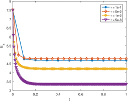
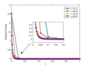
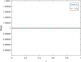
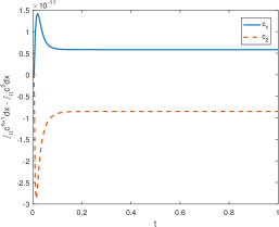
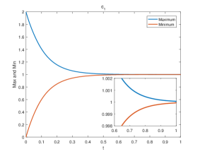
where the initial ionic concentrations are set non-negative. We set and fix the spatial size . Figure 1 plots the time evolutions of the discrete energy (132) and original energy (6) with different time-steps , 0.05, 0.01 and 0.005. We observe that all energy curves decay monotonically for all time-steps, which confirms that the proposed scheme is unconditionally energy stable and the original energy is dissipative. Furthermore, Figure 2 plots the time evolutions of masses , and their errors with . Figure 3 plots the time evolutions of of maximum and minimum values of , with . It is observed that the proposed scheme preserves the properties of mass conservation and positivity during the time evolution.

5 Concluding remarks
In this paper, we constructed first-order fully-decoupled and linearized pressure-correction projection scheme for the NSPNP equations and derived that the proposed scheme is unconditionally energy stable, and preserves non-negativity and mass conservation of the ionic concentration solutions.
We introduced a suitable SAV , which derived from the ionic concentration equations, to treat explicitly the nonlinear terms in the Navier-Stokes part. This allows the nonlinear contributions to the energy to cancel each other out in the continuous case, overcoming the stability condition caused by the temporal discretization [14] of the ionic concentration equations and leading to unconditional energy stability.
We only carry out the rigorous error analysis for the proposed first-order semi-discrete scheme in the two-dimensional case by using mathematical induction on the bounds for and bound for , which are not available through energy stability. Our analysis essentially uses some inequalities that are valid only in two dimensional case, leading to the fact that they cannot be easily extended to the three dimensional case. We shall leave the error estimates in the three dimensional case for future work.
References
- [1] G. Bauer, V. Gravemeier, and W. A. Wall, A stabilized finite element method for the numerical simulation of multi-ion transport in electrochemical systems, Comput. Methods Appl. Mech. Engrg., 223 (2012), pp. 199–210.
- [2] Y.-Z. Chen and L.-C. Wu, Second order elliptic equations and elliptic systems, vol. 174, American Mathematical Society, 1998.
- [3] M. Dehghan, Z. Gharibi, and R. Ruiz-Baier, Optimal error estimates of coupled and divergence-free virtual element methods for the Poisson–Nernst–Planck/Navier–Stokes equations and applications in electrochemical systems, J. Sci. Comput., 94 (2023), p. 72.
- [4] C. Deng, J. Zhao, and S. Cui, Well-posedness for the Navier–Stokes–Nernst–Planck–Poisson system in Triebel–Lizorkin space and Besov space with negative indices, J. Math. Anal. Appl., 377 (2011), pp. 392–405.
- [5] L. Dong, D. He, Y. Qin, and Z. Zhang, A positivity-preserving, linear, energy stable and convergent numerical scheme for the Poisson–Nernst–Planck (PNP) system, J. Comput. Appl. Math., 444 (2024), p. 115784.
- [6] G. Fu and Z. Xu, High-order space–time finite element methods for the Poisson–Nernst–Planck equations: Positivity and unconditional energy stability, Comput. Methods Appl. Mech. Engrg., 395 (2022), p. 115031.
- [7] H. Gao and D. He, Linearized conservative finite element methods for the Nernst–Planck–Poisson equations, J. Sci. Comput., 72 (2017), pp. 1269–1289.
- [8] D. He, K. Pan, and X. Yue, A positivity preserving and free energy dissipative difference scheme for the Poisson–Nernst–Planck system, J. Sci. Comput., 81 (2019), pp. 436–458.
- [9] M. He and P. Sun, Mixed finite element method for modified Poisson–Nernst–Planck/Navier–Stokes equations, J. Sci. Comput., 87 (2021), pp. 1–33.
- [10] J. Hu and X. Huang, A fully discrete positivity-preserving and energy-dissipative finite difference scheme for Poisson–Nernst–Planck equations, Numer. Math., 145 (2020), pp. 77–115.
- [11] M. Li and Z. Li, Error estimates for the finite element method of the Navier-Stokes-Poisson-Nernst-Planck equations, Appl. Numer. Math., 197 (2024), pp. 186–209.
- [12] C. Liu, C. Wang, S. Wise, X. Yue, and S. Zhou, A positivity-preserving, energy stable and convergent numerical scheme for the Poisson-Nernst-Planck system, Math. Comput., 90 (2021), pp. 2071–2106.
- [13] C. Liu, C. Wang, S. M. Wise, X. Yue, and S. Zhou, A Second Order Accurate, Positivity Preserving Numerical Method for the Poisson–Nernst–Planck System and Its Convergence Analysis, J. Sci. Comput., 97 (2023), p. 23.
- [14] X. Liu and C. Xu, Efficient time-stepping/spectral methods for the Navier-Stokes-Nernst-Planck-Poisson equations, Commun. Comput. Phys., 21 (2017), pp. 1408–1428.
- [15] M. S. Metti, J. Xu, and C. Liu, Energetically stable discretizations for charge transport and electrokinetic models, J. Comput. Phys., 306 (2016), pp. 1–18.
- [16] M. Pan, S. Liu, W. Zhu, F. Jiao, and D. He, A linear, second-order accurate, positivity-preserving and unconditionally energy stable scheme for the Navier–Stokes–Poisson–Nernst–Planck system, Commun. Nonlinear Sci. Numer. Simul., 131 (2024), p. 107873.
- [17] A. Prohl and M. Schmuck, Convergent finite element discretizations of the Navier-Stokes-Nernst-Planck-Poisson system, ESAIM: Math. Model. Numer. Anal., 44 (2010), pp. 531–571.
- [18] M. Schmuck, Analysis of the Navier–Stokes–Nernst–Planck–Poisson system, Math. Model Meth. Appl. Sci., 19 (2009), pp. 993–1014.
- [19] J. Shen, T. Tang, and L.-L. Wang, Spectral methods: algorithms, analysis and applications, vol. 41, Springer Science & Business Media, 2011.
- [20] J. Shen and J. Xu, Unconditionally positivity preserving and energy dissipative schemes for Poisson–Nernst–Planck equations, Numer. Math., 148 (2021), pp. 671–697.
- [21] R. Shen and Y. Wang, Stability of the nonconstant stationary solution to the Poisson–Nernst–Planck–Navier–Stokes equations, Nonlinear Anal. Real World Appl., 67 (2022), p. 103582.
- [22] R. Temam, Navier–Stokes equations and nonlinear functional analysis, vol. 66, Society for Industrial and Applied Mathematics, 1995.
- [23] R. Temam, Navier–Stokes equations: theory and numerical analysis, vol. 343, American Mathematical Society, 2001.
- [24] S. Wang, L. Jiang, and C. Liu, Quasi-neutral limit and the boundary layer problem of Planck-Nernst-Poisson-Navier-Stokes equations for electro-hydrodynamics, J. Differ. Equ., 267 (2019), pp. 3475–3523.
- [25] Y. Wang, C. Liu, and Z. Tan, A generalized Poisson–Nernst–Planck–Navier–Stokes model on the fluid with the crowded charged particles: Derivation and its well-posedness, SIAM J. Math. Anal., 48 (2016), pp. 3191–3235.
- [26] Z. Yu, Q. Cheng, J. Shen, and C. Wang, A positivity preserving scheme for Poisson-Nernst-Planck Navier-Stokes equations and its error analysis, arXiv preprint arXiv:2311.17349, (2023).
- [27] X. Zhou and C. Xu, Efficient time-stepping schemes for the Navier-Stokes-Nernst-Planck-Poisson equations, Comput. Phys. Commun., 289 (2023), p. 108763.