Overcoming the Thermal-Noise Limit of Room-Temperature Microwave Measurements by “Cavity Pre-cooling” with a Low-Noise Amplifier
—Application to Time-resolved Electron Paramagnetic Resonance

Abstract

We demonstrate an inexpensive, bench-top method, which we here name “cavity pre-cooling” (CPC), for removing, just prior to performing a measurement, a large fraction of the deleterious thermal photons that would otherwise occupy the electromagnetic modes of a microwave cavity (or some alternative form of rf resonator) at room temperature. Our method repurposes the input of a commercial HEMT-based low-noise amplifier (LNA) to serve as a photon-absorbing “cold load” that is temporarily over-coupled to the cavity. No isolator is inserted between the LNA and the cavity’s coupling port. In a proof-of-concept experiment, the noise temperature of a monitored microwave mode drops from a little below room temperature to $\sim$108 K. Upon incorporating our pre-coolable cavity into a time-resolved (tr-) EPR spectrometer, a commensurate improvement in the signal-to-noise ratio is observed, corresponding to a factor-of-5 speed up over a conventional tr-EPR measurement at room temperature for the same precision and/or sensitivity. Simulations indicate the feasibility, for realistic Q factors and couplings, of cooling the temperatures of a cavity’s modes down to a few tens of K, and for this coldness to last several tens of $\mu s$ whilst the cavity and its contents are optimally interrogated by a microwave tone or pulse sequence. The method thus provides a generally applicable and extremely convenient approach to improving the sensitivity and/or read-out speed in pulsed or time-resolved EPR spectroscopy, quantum detection and other radiometric measurements performed at or near room temperature. It also provides a first-stage cold reservoir (of microwave photons) for deeper cooling methods to work from.

I Introduction

In the face of thermal noise, quantum measurements very often require cryogenic environments to achieve sufficient sensitivity and/or fidelity. In the microwave regime of frequencies, this involves cooling the measuring hardware’s cavities and connecting waveguides down to a temperature of a few tens of mK so as to reliably eliminate the incoherent thermal photons that would otherwise reside within them and wreak havoc. Obeying Bose-Einstein statistics, the expected number of such photons occupying any one of the cavity’s electromagnetic (EM) modes is $\bar{n}=[e^{(hf_{\text{mode}}/k_{\rm B}T})-1]^{-1}$, $f_{\text{mode}}$ being the mode’s frequency. This level of cooling can be achieved, albeit onerously, by installing the hardwave within a deeply cryogenic refrigerator, most often a dilution or adiabatic-demagnetization fridge.

Though currently still a few factors of ten greater in temperature/photon number than what can be achieved through standard mK refrigeration (as involves the removal of thermal phonons from the materials that surround or fill an electromagnetic cavity), recent studies[1, 2, 3, 4, 5] have demonstrated the direct removal of thermal photons from particular microwave modes inside bench-top cavities at room temperature through the stimulated absorption of these photons by an optically spin-polarised medium placed inside the cavity. While obviating the need for physical refrigeration, this hybrid (optical-microwave) approach still requires a sufficiently powerful optical pump source for spin-polarizing the absorbing medium. This results in still quite a bulky and power-hungry system, even when a miniaturized microwave cavity of high magnetic Purcell factor is used to reduce the optical pump power/energy needed[6, 7].

Within microwave instrumentation, low-noise amplifiers (LNAs) are ubiquitously used to boost the power of weak signals. Guided quantitatively by Friis’ formula[8], the deployment of the quietest LNA available at the front end of an instrument’s amplification chain will minimize the amount of deleterious noise added to the measured signal, and so maximize the overall signal-to-noise ratio (SNR) and measurement sensitivity[9]. Compared to their manifest utility in radio-astronomy[10] and deep-space communication[11], the gains in sensitivity from installing a lower-noise (cryogenic) preamplifier into an EPR/NMR spectrometer are found, empirically, to be modest[12, 13, 14], especially when the spectrometer’s microwave/rf cavity is not itself refrigerated, and furthermore dependent on the degree of resonator-amplifier coupling[15].

Various schemes such as Townes’ “Q-multiplier”[16], involving the incorporation of a maser gain medium inside the cavity itself, have been proposed over the years towards improving measurement sensitivity. It was Mollier et al.[17] who cut through the confusion to affirm that, no matter how low-noise the receiving LNA gain medium, the sensitivity of an EPR (or NMR) spectrometer is ultimately limited by thermal noise (i.e. incoherent microwave photons) generated from within the EPR cavity itself. An ultra-low-noise receiving amplifier attached directly to the cavity’s coupling port, or even an ultra-low-noise gain medium resident inside the cavity, will amplify both the signal and this noise equally, thus the SNR won’t improve. As addressed quantitatively by Poole[18] and others[19, 20] since, the only ways to improve sensitivity (for a given sample, completely filling the cavity, at a given temperature) are to either increase the cavity’s quality factor $Q$ (albeit at the expense of measurement bandwidth), so increasing the photon cavity lifetime, or to increase the EPR transition frequency (by applying a strong d.c. magnetic field to the sample), so reducing the number of thermal photons in the cavity’s operational mode. Or else (back to where this argument began:) to physically cool the cavity or otherwise “state-prepare” its operational microwave mode(s).

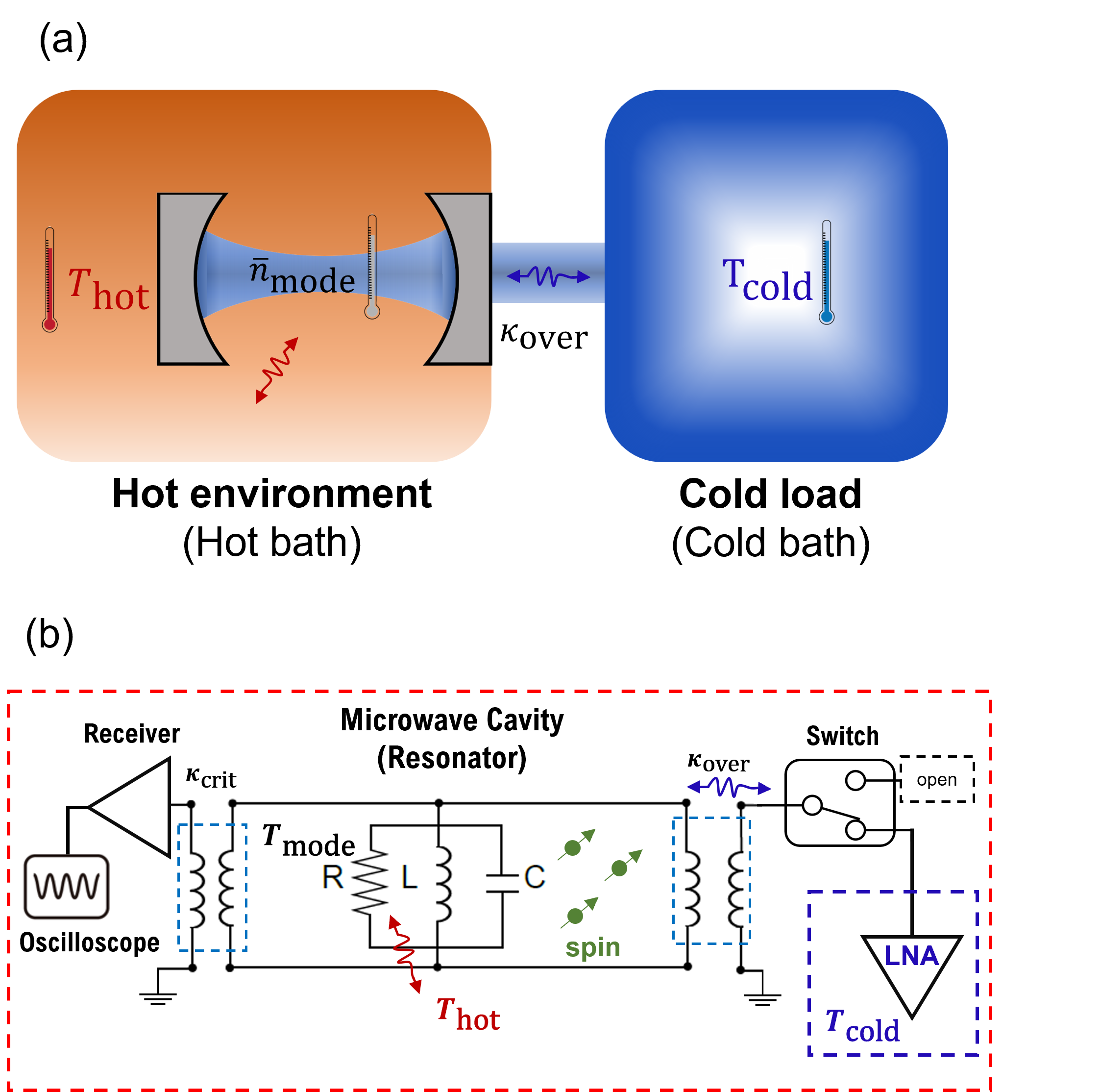
Figure 1: (a) Conceptual mechanism of cavity pre-cooling (CPC): A microwave resonator is physically maintained at a temperature $T_{\text{hot}}$ (in this article, $T_{\text{hot}}$ equals room temperature, denoted as $T_{\text{0}}$) and supports an electromagnet mode whose photon occupation number is $\bar{n}_{\text{mode}}$. This mode is coupled to a cold load maintained at a lower temperature $T_{\text{cold}}$ with a coupling factor of $\kappa_{\text{over}}$ between the load and the mode. (b) Simplified equivalent electrical circuit: The resonator, drawn as an LCR tank circuit, is over-coupled (right) through a (SPDT) switch to either a cold load (in the form of the input of an LNA) or an open circuit -depending on the position of the switch. The mode’s field amplitude (as generates a voltage across the tank circuit) can be measured by a second LNA through its own coupling port (left, usually set to be at critical coupling with the cooling LNA switched out) whose output is recorded on a digital oscilloscope.

At least for frequencies in the low-GHz region, today’s solid-state LNAs, usually in the form of MMICs or hybrids based on InP (or GaAs) HEMTs or else SiGe HBTs, offer impressively low noise temperatures (referred to input) of 50 K or less -even when operating at room temperature. As mature, COTS technologies, they are readily purchasable. If suitably designed/chosen, the noise temperature of such an LNA will decrease by a further order of magnitude or so upon cooling it to liquid-helium temperature[21, 22]. With such low amplifier noise temperatures available, the sensitivity with which the field-amplitude/energy ($=$ number of photons) inside a room-temperature microwave cavity can be measured is determined almost entirely by the cavity’s own thermal noise (as is associated with the rate at which electromagnetic energy is dissipated inside the cavity) -not the small amount of extra noise imparted by the receiving amplifier chain used to monitor the cavity’s field amplitude (through a port attached to the cavity).

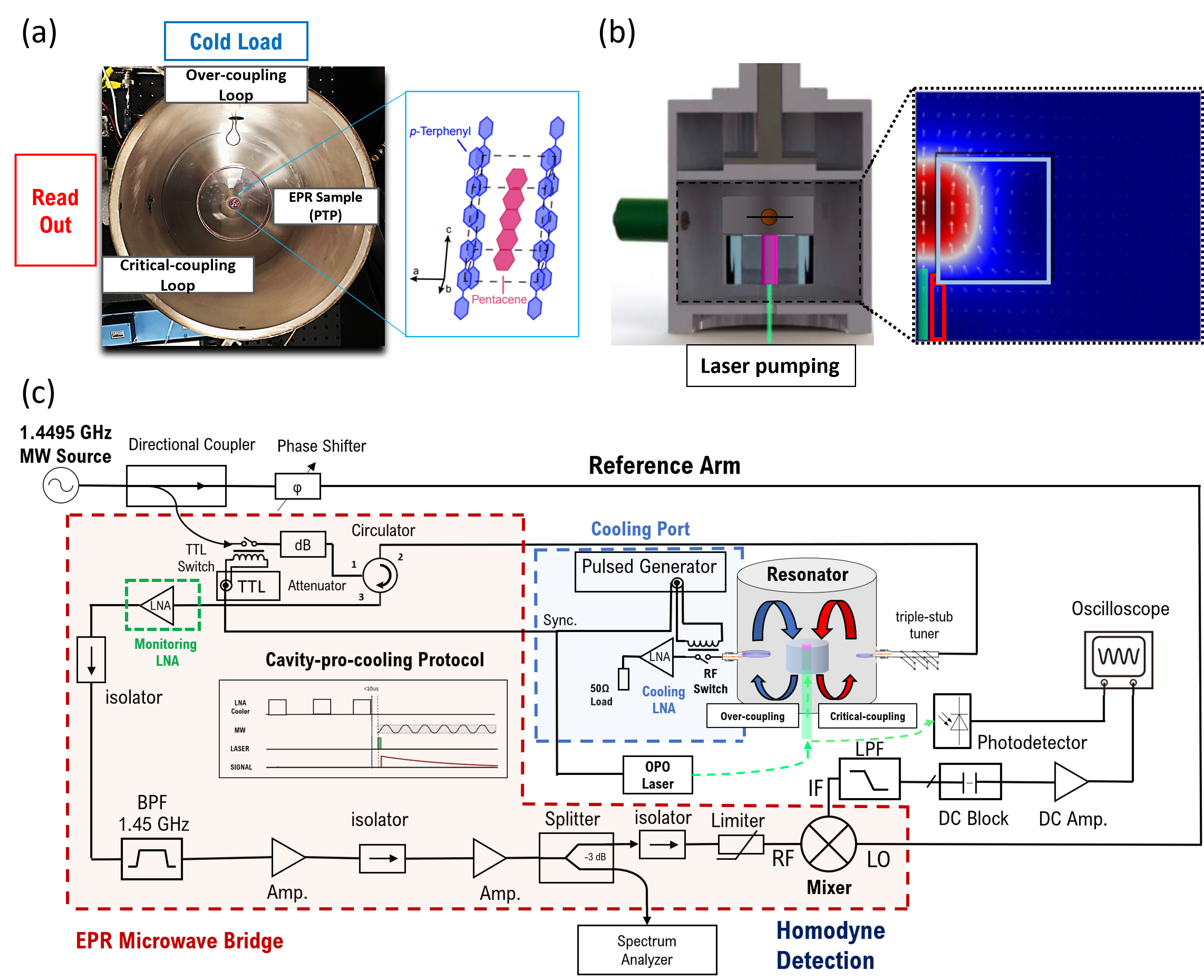
Figure 2: (a) Photograph of the experimental resonator’s insides: a sapphire ring holding a 0.1 % pentacene-doped para-terphenyl (Pc:PTP) crystal, surrounded by the silver-plated walls of a cylindrical brass enclosure. (b) CAD diagram of the same resonator with a two-dimensional axisymmetric simulation of the magnetic flux (white arrows) and magnetic energy density of the TE_01δ microwave mode[23] that this resonator supports. (c) Signal-path anatomy of the experimental tr-EPR spectrometer used to demonstrate cavity pre-cooling. This circuit incorporates homodyne detection of the transient EPR signal. The firing of the OPO laser and the closing/opening of the two microwave switches are scheduled via TTL control pulses (generated by two cascaded pulse generators -both a Thandar TG105) as explained in Fig. 5.

As already mentioned above, Wu et al.[1] demonstrated the cooling of an electromagnetic (EM) mode by coupling it to a “spin-cold” reservoir in the form of an optically excited crystal of pentacene-doped para-terphenyl. Ng et al.[2], Blank et al.[24], and Day et al.[5], have since demonstrated quasi-continuous mode cooling using photoexcited negatively charged nitrogen vacancies (NV^-) in diamond as a spin-polarised absorber. In a similar vein, Englund, Trusheim and co-workers[3, 4] have exploited mode cooling with NV^- diamond to enhance the sensitivity of a magnetometer. All of these works use a cm-sized dielectrically-loaded cavity to support a TE_01δ mode affording a high magnetic Purcell factor. The frequency, $f_{0}$, of the this mode is adjusted or else a d.c. magnetic field is applied, so as to align it with the absorptive paramagnetic transition being targeted. Since the linewidth of this transition is narrow (a few MHz for pentacene, a few hundreds of kHz for NV^- diamond), these approaches to mode cooling are intrinsically narrow-band.

In microwave radiometry, cooled coaxial or waveguide terminations are used as cryogenic loads[25] to absorb unwanted signals and noise. Such a load in combination with a cryogenic circulator (so forming an isolator) is also often used to protect a sensitive quantum circuit from noise back-flowing from a warmer read-out amplifier. In this context, we point out that the cavity-pre-cooling method introduced here draws parallels with the radiatively cooling of a spin ensemble or a resonator, held physically at liquid-helium temperature, by coupling it electromagnetically to an “absorber” (in the form of either a passive load or active device) at mK temperature[26, 27]. A convenient alternative to a physically cryogenic termination is an active cold load (ACL)[28, 29]) which, though a powered device, mimics the former’s behavior. ACLs can be made from the inputs (gates/bases) of suitably biased low-noise transistors [30, 31]. Though not always as cold (nor as broadband or stable) as true cryogenic terminations, they circumvent the need for refrigeration, enabling the advantageous use of ACLs in mobile applications such as the calibration of earth-monitoring radiometers aboard aircraft or satellites[32].

II Cavity Pre-Cooling

The essential idea of the method introduced here is to temporarily cool the EM modes of a room-temperature cavity by (over-)coupling them, temporarily, to an active cold load in the form of the input of a commercial low-noise amplifier (LNA). The output from this LNA does not need to go anywhere at all; it can simply be sunk into a matched passive load or, if the backwards attenuation of the cooling LNA is insufficient, into a second ACL provided by the input of an additional LNA. The method affords wide-band cooling: it will cool all of the modes lying within the LNA’s bandwidth, provided they are overcoupled to the LNA’s input. The concept is shown in Fig. 1. Here, the input of the cooling LNA is temporarily connected via a low-insertion-loss switch to a large loop of wire inside the cavity, which serves as an over-coupled port. This overcoupling ensures that the temperature of a microwave mode (within the LNA’s input bandwidth) is dominated by the LNA’s input noise temperature as opposed to that associated with the cavity’s own intrinsic dissipation (i.e. the temperature at which energy is dissipated in the metal walls and internal dielectric components of the cavity, namely the cavity’s physical ambient temperature). In our proof-of-principle set up here, the temperature of a particular (“target”) mode is monitored through a second port to which the input of a second LNA is critically coupled (once the cooling LNA on the overcoupled port has been disconnected). The output of this monitoring LNA feeds a homodyne receiver tuned to the target mode’s center frequency.

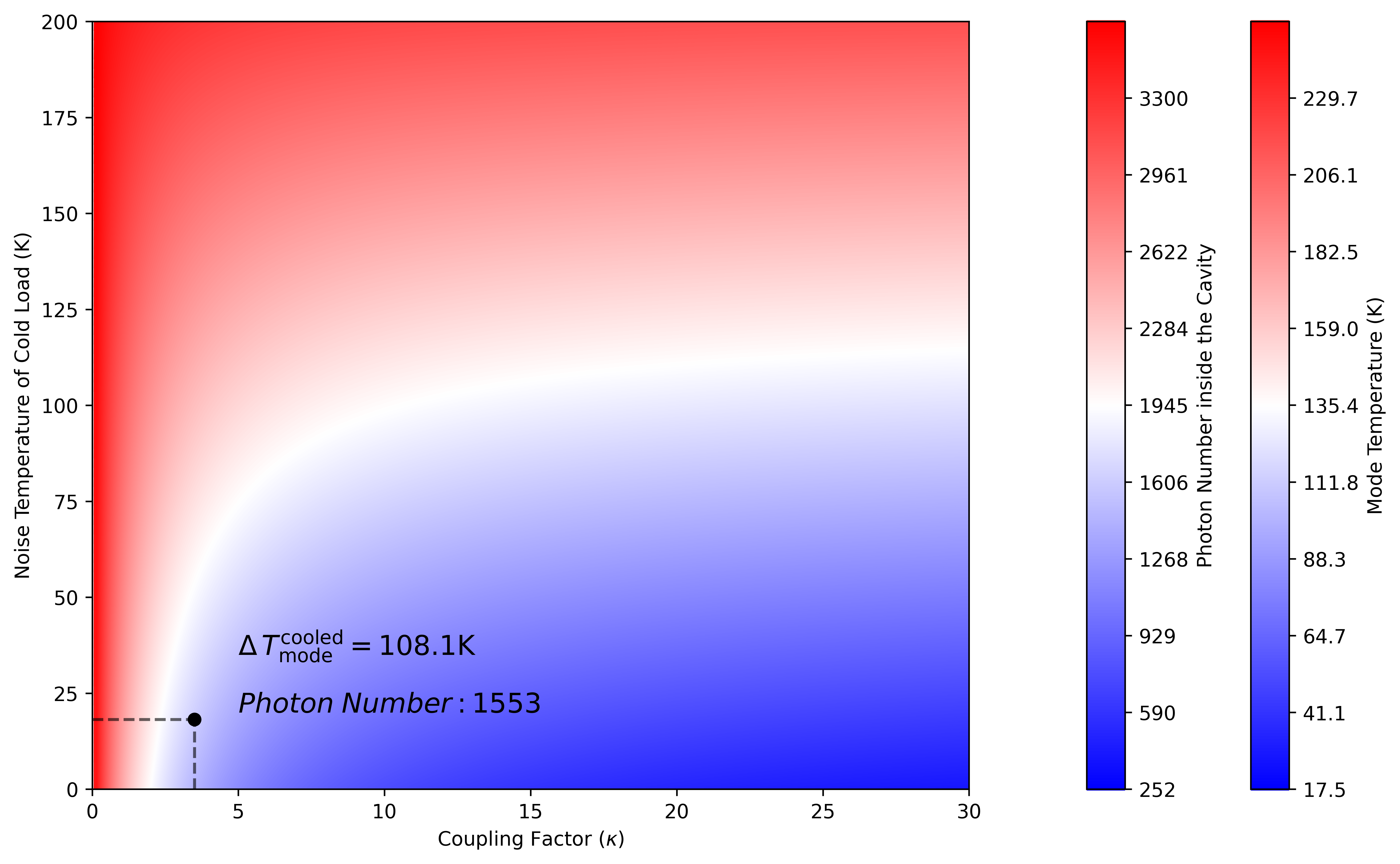
Figure 3: Simulated average number of thermal photons occupying the cavity’s TE_01δ mode and the mode’s corresponding temperature ($T_{\text{mode}}$) as a function of the cold load’s own noise temperature ($T_{\text{cold}}$) and its coupling factor ($\kappa$) to the mode. In our experimental demonstration, this mode’s temperature is reduced from 255.4 K to 108.1 K, the latter temperature corresponding to an average occupancy of 1553 photons.

Details: Our implemented experimental set-up is shown in Fig. 2. However, when solely demonstrating mode cooling, (i) the cavity need not be loaded with an EPR sample, and (ii), the EPR bridge’s circulator can be removed with the monitoring LNA (inside the dashed green box in Fig. 2) connected directly to the critically-coupled port’s stub tuner. Our resonator takes the form of a cylindrical brass cavity, internally plated with silver, whose internal volume is partially filled by a concentrically located ring of monocrystalline sapphire (supplied by J-Crystal Photoelectric Technology, China) whose c-axis lies parallel to the cavity’s axis of rotational symmetry[23]. This ring supports a TE_01δ mode at 1.45 GHz, whose intrinsic quality factor $Q_{\text{cav}}$ = 164,000, providing a loaded quality factor at critical coupling ($\kappa_{c}^{0}=1$) of $Q_{\text{crit.}}=Q_{\text{cav}}/2$ = 82,000. The frequency $f_{0}$ and field profile of this mode were accurately modeled using COMSOL Multiphysics[33]. Unlike the superheterodyne receiver (incorporating a narrowly filtered 70-MHz IF strip) used in the previous cavity-cooling works by Wu and Ng et al. [1, 2], we here use a simpler high-gain homodyne receiver to monitor the amplitude/excitation of the TE_01δ, recording the receiver’s output into a Tektronix TBS 1102B-EDU oscilloscope.

It is worth pointing out that both the cooling and the monitoring of the TE_01δ mode could alternatively be implemented using just a single port attached to a single LNA if this port’s coupling to the mode were made dynamically adjustable, with the LNA alternatively connected (“toggled”), at sufficient speed and glitch-free, between (say) a larger and a smaller coupling loop. However, given that our cavity already had two separate coaxial ports (feedthroughs), it was simpler, with the COTS components immediately available to us, to use both of these ports set to different fixed couplings $\kappa$, namely: (i) an over-coupled “cooling” port ($\kappa_{\text{over}}=3.8$), connected through a low-insertion-loss SPDT switch (viz. a Qorvo RFSW1012) to either the active cold load (viz. the input of a Qorvo QPL9547 LNA mounted on an eval. board) or else an “open” termination -the choice being determined by the control voltage applied to the RFSW1012 switch; and (ii) a “monitoring/interrogation” port, critically coupled ($\kappa_{c}^{0}=1$) to the TE_01δ mode through a Maury Microwave 1819A triple-stub tuner, and used to monitor the mode’s field amplitude (and thus noise temperature). These two different ports are depicted, conceptually, in Fig. 1(b); their experimental embodiments are displayed in Figs 2(a) and 2(c). The coupling factors of both ports (cooling and monitoring) as well as the quality factor of the sapphire resonator’s TE_01δ mode were accurately determined using a trusty HP8753C vector network analyzer (VNA)[34, 35].

What depth of cooling can one expect? From Fig. 1 (a): The microwave cavity (grey) is kept at an intrinsic physical temperature of $T_{\text{hot}}=T_{\text{0}}$ (orangey brown) but the microwave mode that it supports is also coupled, with a coupling factor of $\kappa_{\text{over}}$, to a cold load (blue), whose effective temperature is $T_{\text{cold}}$. On average, $\bar{n}_{\text{mode}}$ thermal photons will occupy the mode, corresponding to a mode temperature of $T_{\text{mode}}=hf_{\text{mode}}/[k_{\rm B}\textrm{ln}(1+1/\bar{n}_{\text{mode}})]$, where

$$T_{\text{mode}}=\frac{T_{\text{0}}+\kappa_{\text{over}}T_{\text{cold}}}{1+\kappa_{\text{over}}}.$$ (1)

One immediately sees from this equation that, if the coupling factor $\kappa_{\text{over}}\gg 1$ (corresponding to a substantially overcoupled port), the microwave cavity’s noise temperature will approach that of the cold load, $T_{\text{cold}}$. In practice, the noise temperature on the over-coupled port as seen/felt by a mode will be slightly higher than the cooling LNA’s input noise temperature due to room-temperature insertion losses (I.L.) between the LNA’s input and the cavity. These losses comprise [see Fig. 2(c)] the I.L. of the SPDT switch itself plus those of the two connecting coaxial cables on either side of it. The increased noise temperature generated by them equals $\lambda T_{\text{0}}$, with $\lambda=L_{\text{dB}}/4.34$, $L_{\text{dB}}$ being the overall I.L. in dB[36]. Furthermore, we need to include the (albeit relatively modest) cooling effect of the critically-coupled monitoring LNA (viz. a second, nominally identical, Qorvo QPL9547EVB-01) that is permanently coupled to the mode. Including all of the above additional contributions (as per Eq. S13 of the Supplementary Material), the lowest obtainable mode temperature, $T_{\text{mode}}^{\text{cooled}}$, is predicted to be

$$T_{\text{mode}}^{\text{cooled}}=\frac{(1+\kappa_{\text{over}}\lambda)T_{\text{0}}+\kappa_{\text{over}}T_{\text{cold}}+T_{\text{mon}}}{2+\kappa_{\text{over}}},$$ (2)

where $T_{\text{mon}}$ is the effective cooling temperature of the monitoring LNA taking into account the unavoidable insertion loss of the triple-stub tuner connecting it to the cavity’s monitoring port, namely $\sim$6 dB, which brings $T_{\text{mon}}$ up to 220.3 K. The expected noise temperature inside the resonator upon pre-cooling, as calculated from Eq. (2) above, is $T_{\text{mode}}^{\text{cooled}}$ = 108.1 K.

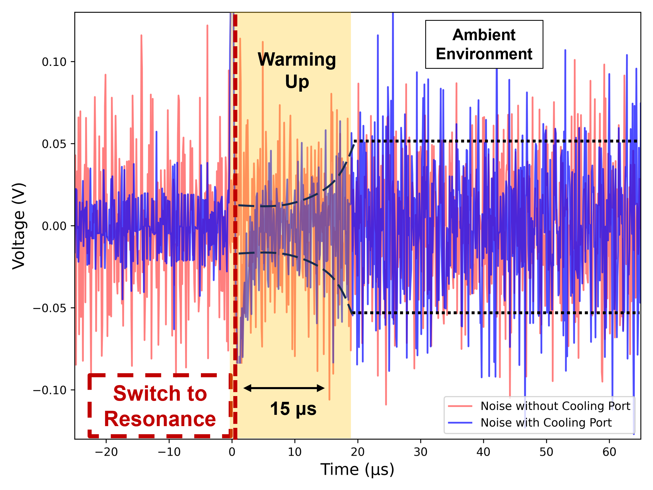
Figure 4: Increase in measured noise over time as the experimental cavity’s monitored microwave mode warms up from “pre-cooled” to ambient conditions. The two black dashed lines track the envelope of the voltage noise. Upon curve-fitting to this envelope (see Fig. 15 in the Supplementary Material), the characteristic time of the warming up is determined to be $\tau_{\text{warm up}}^{\text{exp.}}\approx 9\pm 1\mu$s.

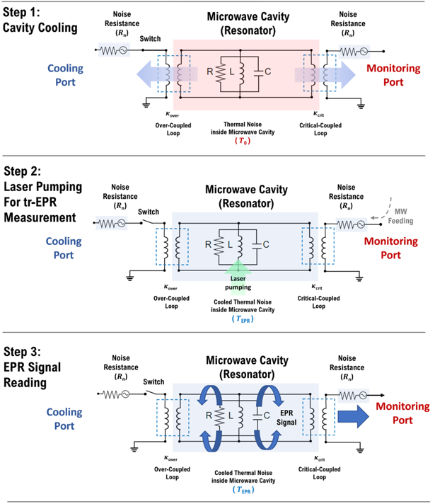
Figure 5: Cavity pre-cooling as applied to time-resolved EPR: In Step 1, an LNA connected to an over-coupled cooling port extracts thermal noise (energy) from the microwave cavity (represented here as an LCR circuit); this also pulls the cavity mode’s resonance frequency $f_{0}$ –slightly. Next (Step 2), a switch disconnects the cooling LNA, bringing the mode back on resonance (i.e., its frequency coincident with the EPR transition’s line center at 1.4495 GHz). Instantaneously with this microwave switching, a q-switched optical pulse (around 7 nanoseconds in duration) of 532-nm pump light is shone on the EPR sample within the the cavity. Subsequently (Step 3), an interrogating coherent microwave tone is applied via a circulator to the cavity’s monitoring port, as shown in Fig. 2 (c), which, upon re-emerging from the cavity through the circulator’s third arm, provides a tr-EPR signal characterizing the EPR sample.

It is worth pointing out how the monitoring LNA itself helps to cool the mode that it monitors. This would not happen if, as is often done, a microwave isolator were inserted between the monitoring LNA and the cavity -so as to “protect” the cavity from external noise. Noise (and thus sensitivity) wise, it is always advantageous to connect the monitoring LNA directly to the cavity so long as its input noise temperature is lower that the physical temperature of the isolator’s internal termination.

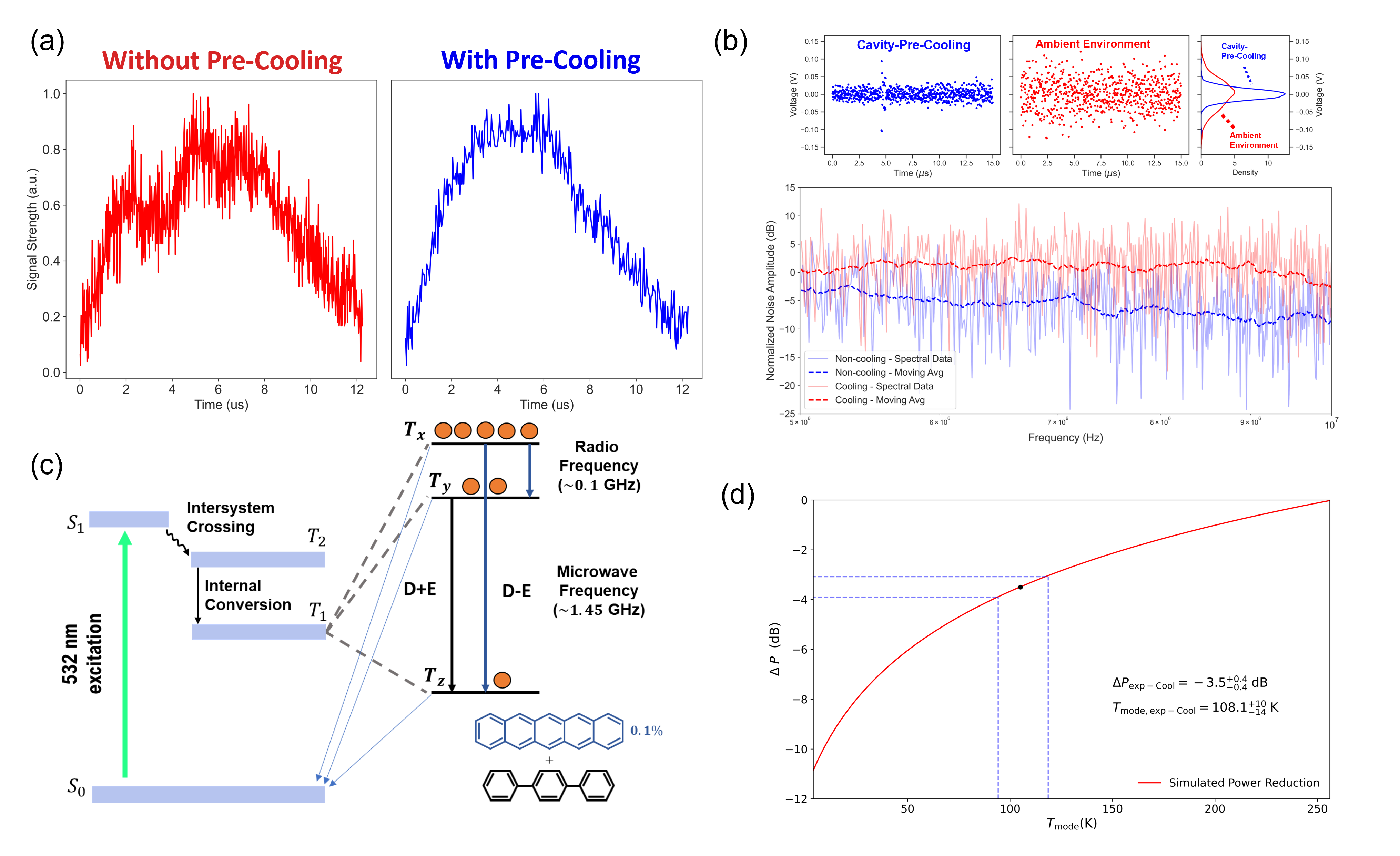
Figure 6: (a) Zero-field tr-EPR signal of Pc:PTP’s $T_{x}-T_{z}$ transition without (red) and with (blue) pre-cooling. (b) Thermal noise (in the time domain) extracted from each of these ZF tr-EPR signals and, below, their corresponding spectral densities; as before, blue and red correspond to the pre-cooled (with) and ambient (without) conditions, respectively. (c) Simplified Jablonski (= energy-level) diagram of the ZF sublevels ($T_{x}$, $T_{y}$, $T_{z}$) of pentacene’s triplet ground state, where D and E denote the ZF splitting (ZFS) parameters. (d) Simulated noise power reduction ($\Delta P$) at the homodyne receiver’s input as a function of the noise temperature of the EPR cavity’s operational mode, $T_{\text{mode}}$. Since its uncertainty is lower, the estimated depth of cooling presented here ($\Delta P_{\text{exp-Cool}}$) corresponds to that achieved by CPC alone (see Table S2 in the Supplementary Material). The depth’s standard error is indicated by dashed cornflower-blue lines.

The reduction in thermal noise will persist so long as the cooling LNA is connected. Upon disconnecting it (so connecting the over-coupling loop to a reflective “open”), the mode regains its higher quality factor, namely $Q_{\text{crit.}}$, and warms up on a timescale set by the mode’s photon lifetime[37], namely $\tau_{\text{warm up}}=\frac{Q_{\text{crit.}}}{2\pi f_{0}}.$ Since the monitoring port is critically coupled to the TE_01δ mode, this mode’s temperature will settle at the (equally weighted) average of $T_{\text{hot}}=290$ K and $T_{\text{mon}}$, namely $T_{\text{mode}}^{\text{ambient}}=255.4$ K for our particular experiment.

III Results

Preliminaries: We determined the noise characteristics of our cooling LNA, namely a Qorvo QPL9547EVB-01 operating at room temperature, using the industry-standard Y-factor method[38]. At 1.45 GHz, it exhibits an impressive noise figure of just 0.26 dB (referenced to 290 K), equivalent to a noise temperature of 18.2 K; see Table S1 in the Supplementary Material for this LNA’s full noise parameters. Experimentally, we observed a reproducible transient on the EPR (homodyne) signal as the SPDT switch opened and disconnected the pre-cooling LNA from the microwave cavity. This artefact (lasting less than 3 $\mu$s in our experiment) could be substantially removed by measuring it for several switch openings then subtracting the average from our measured traces.

Mode Cooling: The effect of connecting then disconnecting the over-coupled cooling LNA to our cavity’s TE_01δ mode at $f_{0}=$ 1.45 GHz is shown in Fig. 4. From the difference in the time average of the measured voltage squared for the mode under cooled and ambient conditions, the depth of cooling is estimated to be $\Delta P_{\text{exp-Cool}}=-3.5\pm 0.4$ dB. This agrees with both our theoretical estimate $\Delta P_{\text{sim}}$ and our analysis using the noise spectrum from experimental tr-EPR data, namely $\Delta P_{\text{exp-EPR}}$, as shown in Fig. 6(b). All our estimates are summarized in Table T2 of the Supplementary Material. Upon curve-fitting to the rise in the measured voltage squared as a function of time, the characteristic time quantifying the persistence of the mode’s coldness after disconnection from the cooling LNA, is estimated to be $\tau_{\text{warm up}}^{\text{exp.}}=9\pm 1~{}\mu$s; see Fig. 15 in the Supplementary Material.

Applicaton to EPR: The protocol used to implement cavity pre-cooling (CPC) is depicted in Fig. 5 and consists of three stages: initial noise extraction via an over-coupled port connected to an active cold load (in the form of the input of an LNA), followed by the disconnection of the ACL, re-tuning the operational mode of the cavity back onto the line center of the target EPR transition, combined with simultaneous laser and microwave excitation to elicit the tr-EPR signal. The process culminates with the signal’s capture through homodyne detection.

To demonstrate the utility of cavity pre-cooling, we studied the SNR and noise spectrum of traces obtained from performing time-resolved EPR on a photo-excited sample of pentacene-doped para-terphenyl (Pc:PTP) at room temperature in zero applied magnetic field. This sample and the complete spectrometer around it are shown in Fig. 2. Fig. 6(a) displays tr-EPR signals for the Pc:PTP triplet’s Tx-Tz transition at 1.4495 GHz [as shown in Fig. 6(c)] both without (red) and with (blue) pre-cooling. The noise on each of the measured tr-EPR signals shown in Fig. 6(a) was extracted from the causal EPR response by first (i) generating a smoothed-out version of the measured data by boxcar averaging, the width of each averaging box being set at 100 ns, then (ii) subtracting this version from the directly measured data to provide the traces shown at the top of Fig. 6(b). Their respective spectral densities (modulus squared of Fourier transform) are displayed underneath. Here, only the section dominated by white noise, above the corner frequency of the observed 1/f noise (at around 1 MHz) generated by the receiver’s LNAs, is shown. These plots attest to the significant reduction in white (thermal) noise that cavity pre-cooling can provide, the SNR (immediately after pre-cooling) being enhanced by $3.5^{+0.4}_{-0.4}$ dB. The relationship between the reduction in the noise power and the achieved noise temperature of the TE_01δ mode at 1.45 GHz is shown in Fig. 6(d). In our demonstration, the mode temperature drops from an initial $T^{\text{ambient}}_{\text{mode}}=255.4$ K to a pre-cooled $T_{\text{mode}}^{\text{cooled}}=108.1$ K, corresponding to a reduction in the expected number of thermal photons from 3669 to 1553. The plot shown in Fig. 3 indicates that, at room temperature, the number of thermal photons in a mode at $1.45\,\text{GHz}$ can be reduced to just a few hundred (cf. ref. [39]) given a sufficiently over-coupled port ($\kappa_{\text{over}}>10$) and quiet LNA ($T_{\text{cold}}<20\,\text{K}$).

Restricting ourselves to work done on bench-tops at room temperature, we here briefly compare the performance achieved by our demonstration of CPC to that achieved by removing thermal photons via stimulated absorption in an absorptively spin-polarised medium resident inside the cavity; in the literature, this latter approach has been dubbed “masar”[1] or “anti-maser”[24]. Using photo-excited pentacene-doped para-terphenyl as the absorber, Wu et al.[1] cooled a TE_01δ mode at 1.45 GHz down to around 50 K -though only in bursts. Using NV^- diamond, Ng et al.[2] and Day et al.[5] cooled the same type of mode continuously to 188 K at 2.9 GHz and to 70 K at 9.8 GHz, respectively. Given that these temperatures straddle what we here achieve using CPC, one may conclude that, currently, there is no clear winner. Both approaches can assuredly be improved upon through focussed material science and device engineering. Beyond cost and convenience, a salient advantage of CPC is that the disturbance on the microwave cavity imposed by the cooling mechanism can be removed at the flick of a (microwave) switch. Methods based on internal stimulated absorption are, in contrast, beholden to the particular spin dynamics of the cooling medium. One could however use an external masar/anti-maser (operated either CW or quasi-continuously[40]) as the active cold load (ACL) to implement CPC instead of a HEMT-based LNA, with the connection between the resonator and the anti-maser’s coupling port gated by the microwave switch. As with other pulse-based techniques at microwave frequencies, a successful implementation of CPC relies heavily on the availability of a sufficiently fast, low-loss and glitch-free switch.

To conclude, we have demonstrated a method for pre-cooling the modes of a microwave cavity by temporarily over-coupling them to the input of an LNA serving as an active cold load (ACL). Beyond tr-EPR, other pulsed-EPR techniques such as ESEEM, HYSCORE, and PELDOR could be accelerated by CPC, reducing measurement times[18]. Furthermore, our analysis evaluates how an LNA that is (either continuously or intermittently) coupled directly to the cavity (i.e. with no “protective” isolator inserted in-between) can play an active and beneficial role in reducing the number of thermal photons occupying the cavity’s modes (within the LNA’s bandwidth) -as opposed to just being a passive monitor.

The use of cryogenic ACLs, operating at (say) liquid-helium temperature yet providing input noise temperatures and thus mode cooling down into the mK regime, is perfectly conceivable. Unfortunately, due to self-heating within the device’s active channel/layer, the noise temperatures of what are currently the best semiconductor-based LNAs hit, upon cooling, plateaux of a few K [41, 42]. The construction of effective cryo-ACLs to achieve mK-level mode cooling may thus require new materials and/or architectures (and the associated investment in fabrication equipment to realize such) optimized expressly for mode-cooling –as opposed to the hacking/repurposing of commercially available devices, designed to do something else, like what we have done here. At a more general, sociologically level, it is hoped that this paper induces greater cross-fertilization between pockets of wisdom lurking within microwave radiometry[43], activities across the EPR/NMR communities[44], and hardware innovations in quantum computing/detection (particularly those targeting room-temperature operation)[45].

Acknowledgements: The authors would like to thank Wern Ng and in particular Hao Wu, now at the Beijing Institute of Technology (BIT), for helpful discussions. This work was supported by the U.K. Engineering and Physical Sciences Research Council through Grants Nos. EP/K037390/1 and EP/M020398/1. K.C. acknowledges financial support from the Taiwanese Government Scholarship to Study Abroad (GSSA).

*

Appendix A SUPPLEMENTARY MATERIAL

A.1 EXPERIMENTAL METHOD - DETAILS

The anatomy of the microwave cavity used in our zero-field tr-EPR spectrometer for cavity pre-cooling demonstrations is shown in Fig. 7. This cavity supports a $\textrm{TE}_{01\delta}$ mode at 1.4495 GHz, exhibiting a loaded quality factor of $Q_{\text{loaded}}=82,000$ when critically coupled, corresponding to an unloaded quality factor of $Q_{0}=164,000$. The cavity consists of five main components: (i) a cylindrical brass enclosure, whose internal walls are plated with silver, (ii) a monocrystalline sapphire ring (supplied by J-Crystal Photoelectric Technology, China) exhibiting low dielectric loss, (iii) an EPR sample, namely a 0.1% pentacene-doped para-terphenyl (PC: PTP) crystal, located in the ring’s bore, (iv) an over-coupling loop (coupling factor = 3.8) connected through a single-pole-double-throw (SPDT) RF switch (viz. a Qorvo RFSW1012PCK-411 eval. board) to a low-noise amplifier (= LNA, viz. a Qorvo QPL9547EVB-01 eval. board), functioning as an active cold load, and (v) a critical-coupling loop connected, via a stub tuner, to a second identical LNA (another QPL9547EVB-01), functioning as the front-end pre-amplifier of a tuned homodyne receiver. The sample receives a Q-switched optical pulse at 532 nm, approximately 5.5 ns in duration and 2 mJ in energy, at a 10 Hz repetition rate, from an integrated Nd:YAG pumped Type II BBO OPO (viz. a Litron Aurora II Integra).

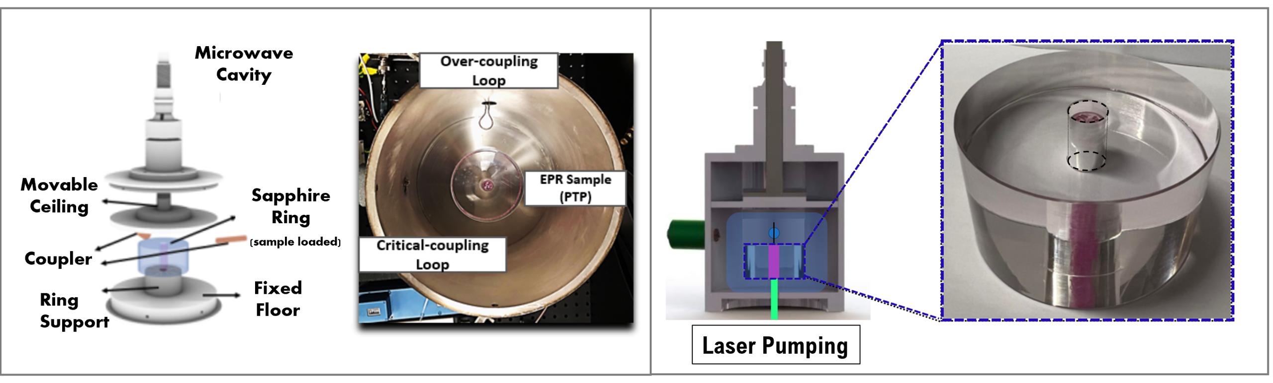
Figure 7: The left image presents the 3D CAD assembly of the microwave cavity (without microwave walls), featuring a movable “ceiling” (= plunger), raised and lowered by a rotating a helical screw (to which the ceiling is mechanically attached) seated in a matching helical thread tapped into the cavity’s “roof” along the cavity’s cylindrical axis. The photo to the right of the drawing shows the cavity’s innards with the ceiling and roof removed. The cavity includes two ports: an over-coupling loop (at 12 o’clock in the photo) and a smaller critical-coupling loop (at 9 o’clock) just poking out of the cavity’s internally-silver-plated wall. The right figure displays the microwave cavity in 2D cross-section. Here, the high-Q sapphire ring is located concentrically on top of a cross-linked polystyrene stand (not shown); its on-axis bore hole, 10 mm in diameter, is filled with the EPR sample (a 0.1% PC:PTP crystal).

The cavity’s internal cylindrical sapphire ring measured 40 mm in height with outer and inner diameters of 68 mm and 10 mm, respectively. The optical “c”-axis of the sapphire (a monocrystal) was aligned with the cylindrical axis. By rotating a screw, the cavity’s axial length (i.e. the internal height of the cavity’s ceiling above its “floor”) could be varied from 150 mm down to 95 mm, allowing wide adjustment in the frequency of the cavity’s $\textrm{TE}_{01\delta}$ mode. The sapphire ring’s hollow supporting pillar was made of cross-linked polystyrene, a solid material offering both low dielectric loss and, unlike PTFE or polyethylene, precision-machineability. This pillar was securely seated into a central hole in the cavity’s floor, holding the sapphire ring 16 mm above the floor. The pillar’s bore allowed for the transfer of pump light, up the cavity’s axis, to the EPR sample. The cavity’s silvered internal surfaces were finely buffed with an abrasive pad, removing patina, then solvent-wiped clean, to leave a gleaming finish.

By constructing a suitable model in COMSOL Multiphysics (a finite-element-based PDE solver) [33], the magnetic mode volume $V_{\text{mode}}$ of the microwave cavity’s $T_{01\delta}$ mode was calculated to be 29 cm³. Experimentally, using a vector network analyser (= VNA, viz. an HP-8753C), the cavity’s loaded quality factor ($Q_{\text{loaded}}=82,000$) and the coupling factors of each of its two ports ($\kappa_{\text{over}}=3.8$, $\kappa_{\text{crit}}=1$) were inferred by the method(s) of Kajfez and Hwan [34]. The PC:PTP crystal, used as our tr-EPR test sample, was grown by the vertical Bridgman method; it fitted into the 10-mm bore of the sapphire ring. The pulsed optical beam from a Q-switched OPO was directed into the microwave cavity via a multimode optical fiber, entering through an 8-mm hole in the centre of the cavity’s floor.

The homodyne receiver for our tr-EPR measurements used a setup akin to Wu et al.’s previous work [50], albeit with the microwave cavity (resonator) now connected to an additional port (for cooling) and with additional routing switches and associated synchronization circuitry -see Fig. 2(c) in the main paper and Fig. 8 below. A sync. pulse from the OPO’s Q-switch driver is used to trigger two pulse generators [both Thandar TG105, one triggered by (= “slaved to”) the other] providing appropriate TTL voltage transitions (“edges”) to connect/disconnect the precooler and switch on/off the EPR spectrometer’s interrogating microwave tone. The most critical switch, needed to perform a clean, abrupt disconnect of the precooling LNA, was a Qorvo RFSW101 SPDT switch, chosen for its low insertion loss, high isolation and sufficient speed; this routes the cooling port’s over-coupling loop first to the active cold load (embodied as the input of a Qorvo QPL9547 LNA) for cooling and, subsequently, to an “open” load (reflecting power back into the cavity, effectively neutralizing the port) for the tr-EPR measurement, when the interrogating microwave tone is applied through the cavity’s critically-coupled monitoring port. To achieve sufficient measurement sensitivity, the homodyne receiver employs a cascade of legacy r.f. amplifiers (total gain $\approx 70$ dB). Upon mixing (= homodyning) down to baseband, the transient tr-EPR signal is channeled (via a DC block) into a fast DC amplifier (viz. a Comlinear E103-I-BNC). All components operate under ambient lab conditions.

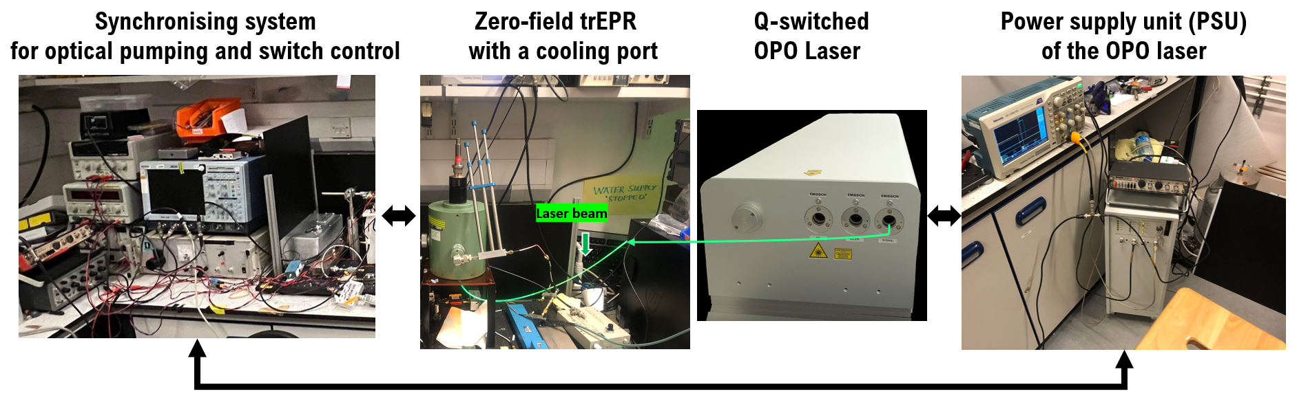
Figure 8: The experimental rig (here emphasizing its electrical synchronization and light path) encompassing, from right to left: the OPO’s power supply unit (PSU), the OPO laser head itself, the resonator and it surrounding microwave “plumbing", and the tr-EPR spectrometer’s support electronics.

A.2 CONCEPT AND MODEL OF THE CAVITY-PRE-COOLING TECHNIQUE

A.2.1 Number of photons inside a microwave cavity

Obeying Bose-Einstein statistics, the average number of photons, $\bar{n}$, occupying an electromagnetic mode of frequency $f_{\text{mode}}=\omega_{\text{mode}}/(2\pi)$ inside an isolated (zero ports) cavity maintained at a physical temperature of $T_{0}$, is given by $\bar{n}=\left[\exp\left(\frac{hf_{\text{mode}}}{k_{\text{B}}T_{0}}\right)-1\right]^{-1}$, where $k_{\text{B}}$ and $h$ are Boltzmann’s and Planck’s constants, respectively. Semiclassically, for a microwave cavity with a single port coupling it to an external cold load, as depicted schematically in Fig. 9, the number of photons $q$ occupying the mode as a function of time $t$ will obey

$$\frac{\text{d}q}{\text{d}t}\equiv\dot{q}=\underbrace{-\omega_{\text{mode}}Q_{0}^{-1}(q-\epsilon T_{0})}_{\hbox{\pagecolor{red}interaction with intrinsic ``hot'' heat bath}}-\underbrace{\omega_{\text{mode}}\kappa Q_{0}^{-1}(q-\epsilon T_{\text{cold}})}_{\hbox{\pagecolor{cyan}interaction with external ``cold'' heat bath}},$$ (3)

where the value of the constant $\epsilon=\frac{k_{\text{B}}}{hf_{\text{mode}}}$ respects Maxwell-Boltzmann equipartition of energy[1]. $T_{\text{cold}}$ is the noise temperature of the active cold load used in the experiment; $Q_{0}$ and $Q_{\text{loaded}}$ are the intrinsic and loaded quality factors of the microwave cavity, where $Q_{\text{loaded}}=\frac{Q_{0}}{1+\kappa}$; $\kappa$ is the port’s coupling factor. This formula can be trivially extended to include additional ports coupling the microwave mode at different couplings strengths $\kappa_{i}$ to additional loads at different temperatures $T_{i}$:

$$\dot{q}=-\underbrace{\omega_{\text{mode}}Q_{0}^{-1}(q-\epsilon T_{0})}_{\hbox{\pagecolor{red}intrinsic bath}}-\sum_{i=1}\underbrace{\omega_{\text{mode}}\kappa_{i}Q_{0}^{-1}(q-\epsilon T_{i})}_{\hbox{\pagecolor{cyan}external bath(s)}}.$$ (4)

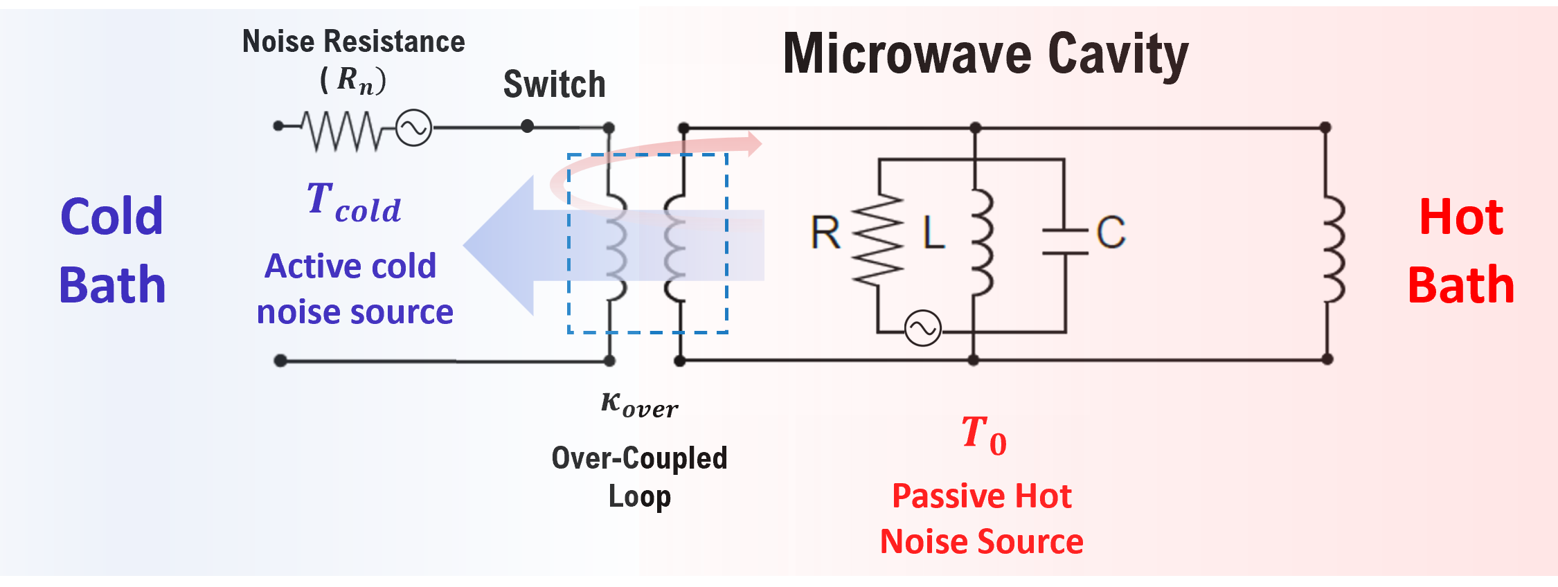
Figure 9: The cavity pre-cooling technique involves electromagnetically coupling a resonator, that is physically heat-sunk to a room-temperature environment (here referred to as the “hot bath”), to an active cold noise source or “load”, here functioning as a “cold bath”.

A.2.2 Mode temperature inside the cavity

Upon achieving dynamic equilibrium, $\dot{q}=0$, the rate equation in Eq. 3 can thereupon be used to calculate the expected photon number. Defining the mode’s equivalent temperature as $T_{\text{mode}}=\frac{q}{\epsilon}=\frac{qhf_{\text{mode}}}{k_{\text{B}}}$, we obtain, for a single coupling port:

$$T_{\text{mode}}=\frac{T_{0}+\kappa T_{\text{cold}}}{1+\kappa}.$$ (5)

In words: the mode’s expected temperature is the weighted average temperature of the two baths with which the mode interacts, the weighting of each bath being proportional to its interaction strength with the mode, i.e. its “coupling”. Here, the coupling of the mode to the cavity’s own intrinsic heat bath is (by definition/convention) unity. Fig. 10 displays the mode temperature predicted by Eq. 5. When the coupling factor of the over-coupling loop $\kappa$ is large, the mode temperature $T_{\text{mode}}$ will approach that of the cold load $T_{\text{cold}}$.

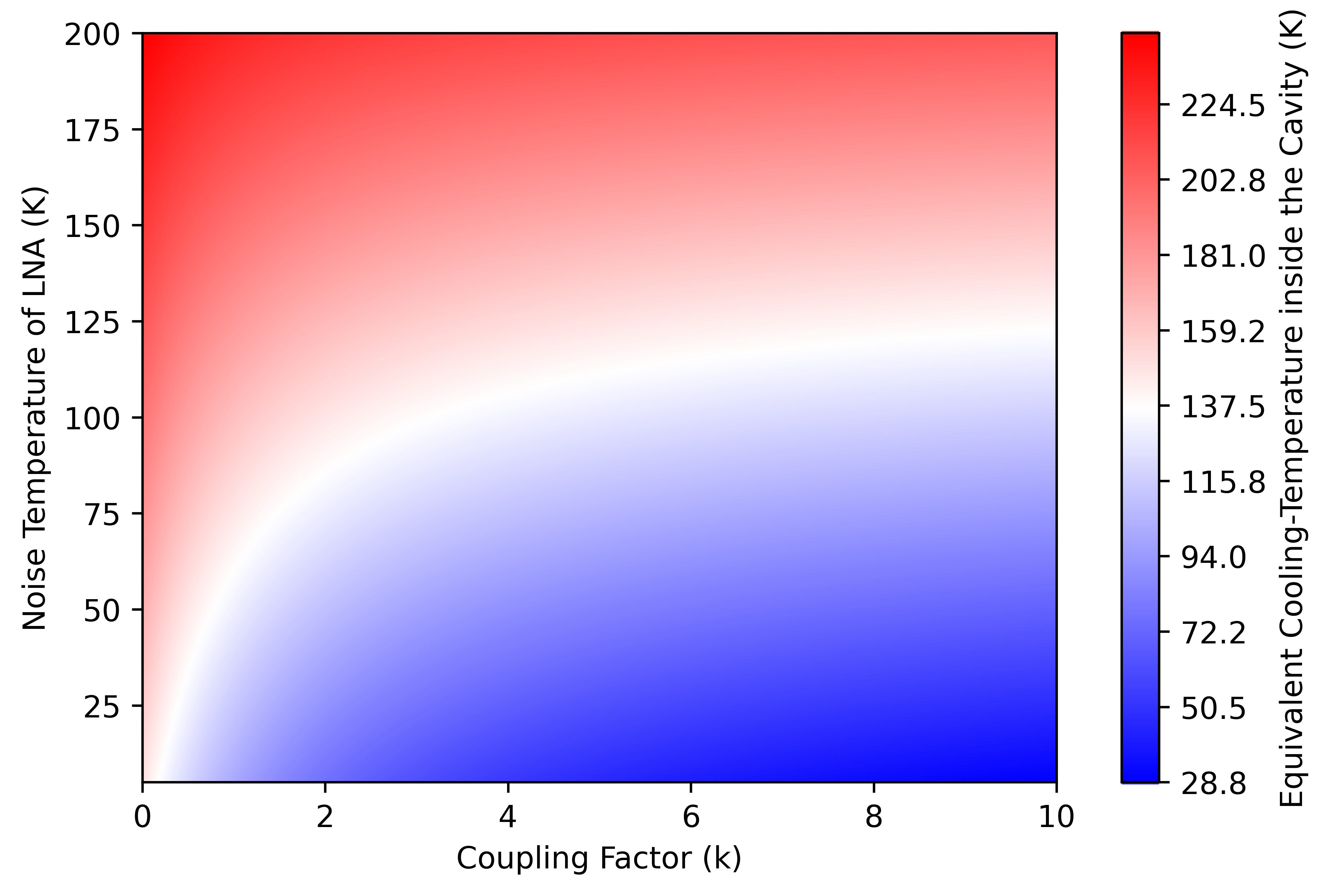
Figure 10: Simulated equivalent temperature of an electromagnetic mode inside the cavity as a function of the coupling factor $\kappa$ (horizontal coordinate) and the noise temperature of the cold load $T_{\text{cold}}$ coupled to this mode (vertical coordinate).

A.2.3 Cavity cooling via a lossy transmission line

The input of a low-noise amplifier (LNA) can serve as an active cold load for reducing the thermal noise inside a cavity that is coupled to it. Here we analyse the additional thermal noise generated by a lossy transmission line, such as a length of coaxial cable, or any other lossy component inserted between the cold load and the cavity, as shown generically in Fig. 11. See Chapter 8 of Ref. [36] for the conceptual foundations and mathematics of the “wave approach”[52] used here.

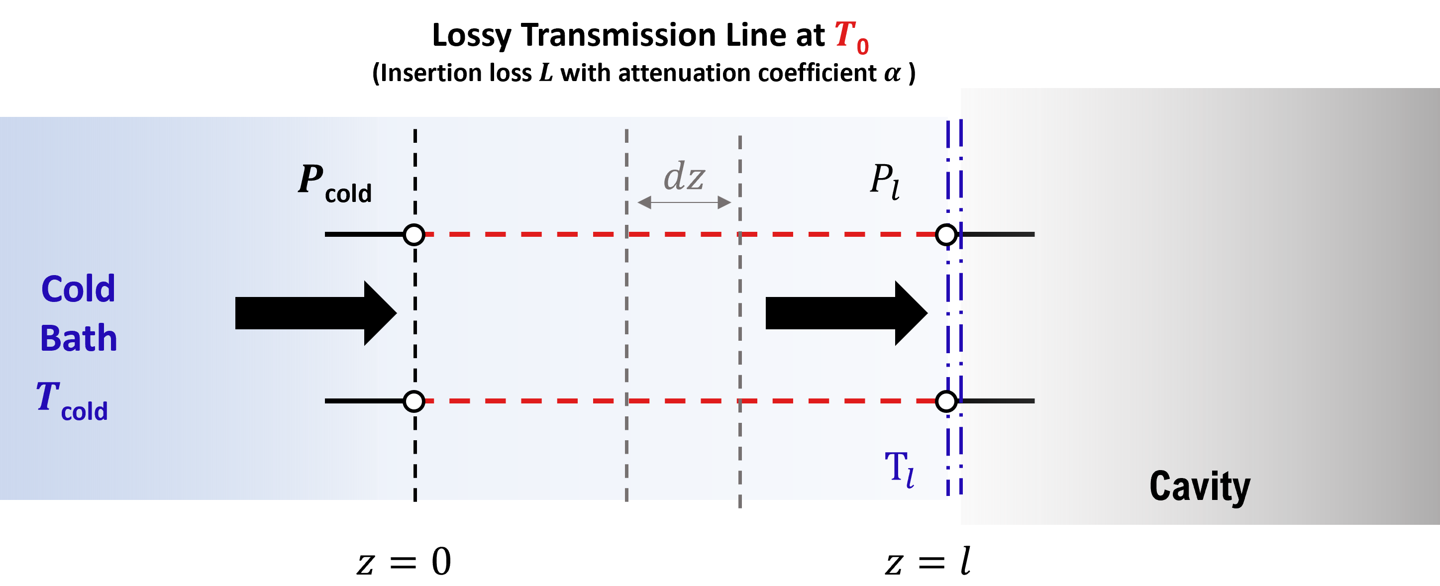
Figure 11: Calculating how the cooling LNA’s noise temperature is degraded by transport along a length of (warm) lossy transmission line.

For initial simplicity, let’s assume that the transmission line is uniform and held at a constant physical temperature $T_{0}$ along its length. The power $P_{\text{sig}}$ of a signal flowing down such a line will decrease exponentially with distance obeying $dP_{\text{sig}}/dz=-2\alpha P_{\text{sig}}$, where $\alpha$ is the line’s voltage attenuation coefficient. Not only is the signal attenuated, but thermal noise is generated along the lossy line’s length. At a distance $z=l$ from the cold load, the forward-traveling noise power $P_{l}$ will equal

$$P_{l}=LP_{\text{cold}}+(1-L)P_{\text{line}},$$ (6)

where $P_{\text{cold}}$ and $P_{\text{line}}$ are the available noise powers from a cold load at temperature $T_{\text{cold}}$ and the end of an infinite length of the lossy transmission line at temperature $T_{0}$, respectively; $L$ is the insertion loss of the line between the cold load and the observation point at $z=l$, where $L=e^{-2\alpha l}$ and $L\leq 1$. Across a given frequency band of width $B$, $P_{\text{line}}=k_{\text{B}}T_{\text{line}}B$ (for $hf/kT\ll 1$).

In the case of a short transmission line (or any other 2-port component) with minimal insertion loss, such that $L\approx(1-2\alpha l)$ to good approximation, the equivalent noise power $P$ at the end of the transmission line can be approximated (expressing the line’s attenuation in decibels) as:

$$P_{l}=(1-\frac{L_{\text{dB}}}{4.34})P_{\text{cold}}+\frac{L_{\text{dB}}}{4.34}P_{\text{line}}.$$ (7)

Note that this (slightly more complicated) approximation is more accurate than equation (8-2-5) in Siegman’s book [36]. Based on the relation between noise power and noise temperature, namely $P=k_{\text{B}}TB$, the effective noise temperature of the cold load, upon including the additional noise from a lossy transmission line connected to it, can thereupon be approximated as:

$$T_{l}=(1-\frac{L_{\text{dB}}}{4.34})T_{\text{cold}}+\frac{L_{\text{dB}}}{4.34}T_{0},$$ (8)

where $T_{\text{cold}}$ the temperature of the cold load itself and $T_{0}=T_{\text{line}}$ is the (here assumed to be room) temperature of the transmission line. Combining Eq. 5 and Eq. 8, the mode’s noise temperature inside the microwave cavity is now given by:

$$T^{\prime}_{\text{mode}}=\frac{T_{0}+\kappa[(1-\frac{L_{\text{dB}}}{4.34})T_{\text{cold}}+\frac{L_{\text{dB}}}{4.34}T_{0}]}{1+\kappa}=T_{\text{mode}}^{\text{orig.}}+\Delta T_{\text{link}},$$ (9)

where $T_{\text{mode}}^{\text{orig.}}$ is the original mode temperature as given by Eq. 5 above and $\Delta T_{\text{link}}=\frac{L_{\text{dB}}}{4.34}\kappa(T_{0}-T_{\text{cold}})/(1+\kappa)$ is the added noise temperature caused by the lossy transmission line.

A.2.4 Multiple cooling ports to a microwave cavity

We now consider a microwave cavity with two ports, one for cooling, the other for read-out, connected to separate LNAs functioning as cold loads. With the setup depicted in Fig. 12 and applying Eq. 4, the rate equation governing the microwave cavity’s photon number is:

$$\dot{q}=-\underbrace{\omega_{\text{mode}}Q_{0}^{-1}(q-\epsilon T_{0})}_{\hbox{\pagecolor{red}Hot bath}}-\underbrace{\omega_{\text{mode}}(Q_{0}/\kappa_{\text{over}})^{-1}(q-\epsilon T_{\text{cold}})}_{\hbox{\pagecolor{cyan}Cold bath of cooling port}}-\underbrace{\omega_{\text{mode}}(Q_{0}/\kappa_{\text{crit}})^{-1}(q-\epsilon T_{\text{cold}})}_{\hbox{\pagecolor{cyan}Cold bath of monitoring port}},$$ (10)

where $\kappa_{over}$ and $\kappa_{crit}$ ($\kappa_{crit}$ = 1) are the coupling factors of the over-coupled and critically-coupled loops, respectively. Analogous to the simpler derivation in the previous mode-temperature analysis above, in dynamic equilibrium when $\dot{q}=0$, the depth of the obtainable cavity cooling can be deduced. The mode temperature $T_{\text{mode}}$ of the system, shown in Fig. 12, is given by:

$$T_{\text{mode}}=\frac{T_{0}+(\kappa_{\text{over}}+\kappa_{\text{crit}})T_{\text{cold}}}{1+\kappa_{\text{over}}+\kappa_{\text{crit}}}=\frac{T_{0}+(1+\kappa_{\text{over}})T_{\text{cold}}}{2+\kappa_{\text{over}}}.$$ (11)

In general, the temperature of a mode of a cavity with multiple cooling ports can be expressed as a weighted average:

$$T_{\text{mode}}=\frac{T_{0}+\sum_{i=1}^{n}\kappa_{i}T_{i}}{1+\sum_{i=1}^{n}\kappa_{i}},$$ (12)

where $\kappa_{i}$ and $T_{i}$ represent the coupling factor and noise temperature of the $i$-th cooling (or warming) element coupled to the mode, respectively.

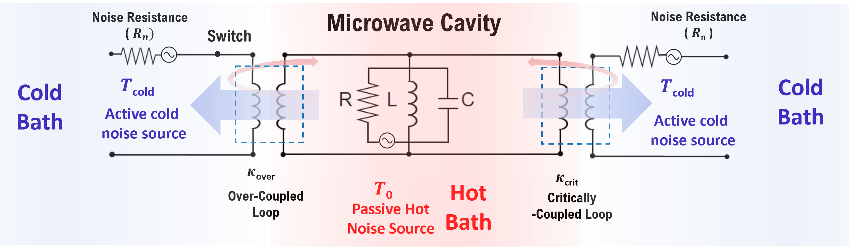
Figure 12: Cavity cooling with two separate cold baths.

A.2.5 Multiple cooling ports to a microwave cavity with lossy transmission lines

In this section, we consider a microwave cavity with multiple cooling ports and lossy transmission lines, integrating concepts from sections 2.3 and 2.4. Combining equations Eq. 8 and Eq. 12, yields

$$T_{\text{mode}}=\frac{T_{0}+\kappa_{1}[(1-\frac{L_{\text{dB,1}}}{4.34})T_{\text{cold}}+\frac{L_{\text{dB,1}}}{4.34}T_{0}]+\kappa_{2}[(1-\frac{L_{\text{dB,2}}}{4.34})T_{\text{cold}}+\frac{L_{\text{dB,2}}}{4.34}T_{0}]}{1+\kappa_{1}+\kappa_{2}},$$ (13)

where $\kappa_{1}$ and $\kappa_{2}$ represent the coupling coefficients of the first and second cold baths, respectively. We here assume the insertion losses of the transmission lines associated with the cold baths ($L_{\text{dB,1}}$, $L_{\text{dB,2}}$) are small. If however the insertion loss of a connecting cable/device is not small, one needs to revert back to Eq. 6, equivalent to equation in (8-2-4) in Siegman’s book [36]. Based on the relation between noise power and noise temperature, $P=k_{\text{B}}TB$, the equivalent noise temperature of a cold load at temperature $T_{\text{cold}}$, observed through a length of transmission line at temperature $T_{0}$ and of significant linear insertion loss $L=10^{-L_{\text{dB}/10}}$, can be quantified as:

$$\begin{split}T_{l}&=LT_{\text{cold}}+(1-L)T_{0}\\ &=10^{-\frac{L_{\text{dB}}}{10}}T_{\text{cold}}+\left(1-10^{-\frac{L_{\text{dB}}}{10}}\right)T_{0}.\end{split}$$ (14)

Our experimental set-up includes two cold baths: one of them, namely the input of the cooling LNA, is connected to the cavity (when selected by the SPDT switch) via a small insertion loss, whereas the other heat bath, namely the monitoring LNA’s input, is connected to the cavity via a large insertion loss. The most appropriate formula for calculating the temperature of the cavity’s operational mode is thus:

$$T_{\text{mode}}=\frac{T_{0}+\kappa_{1}[(1-\frac{L_{\text{dB,1}}}{4.34})T_{\text{cold}}+\frac{L_{\text{dB,1}}}{4.34}T_{0}]+\kappa_{2}[10^{-\frac{L_{\text{dB,2}}}{10}}T_{\text{cold}}+(1-10^{-\frac{L_{\text{dB,2}}}{10}})T_{0}]}{1+\kappa_{1}+\kappa_{2}}.$$ (15)

These approximations are analyzed in Fig. 13 below.

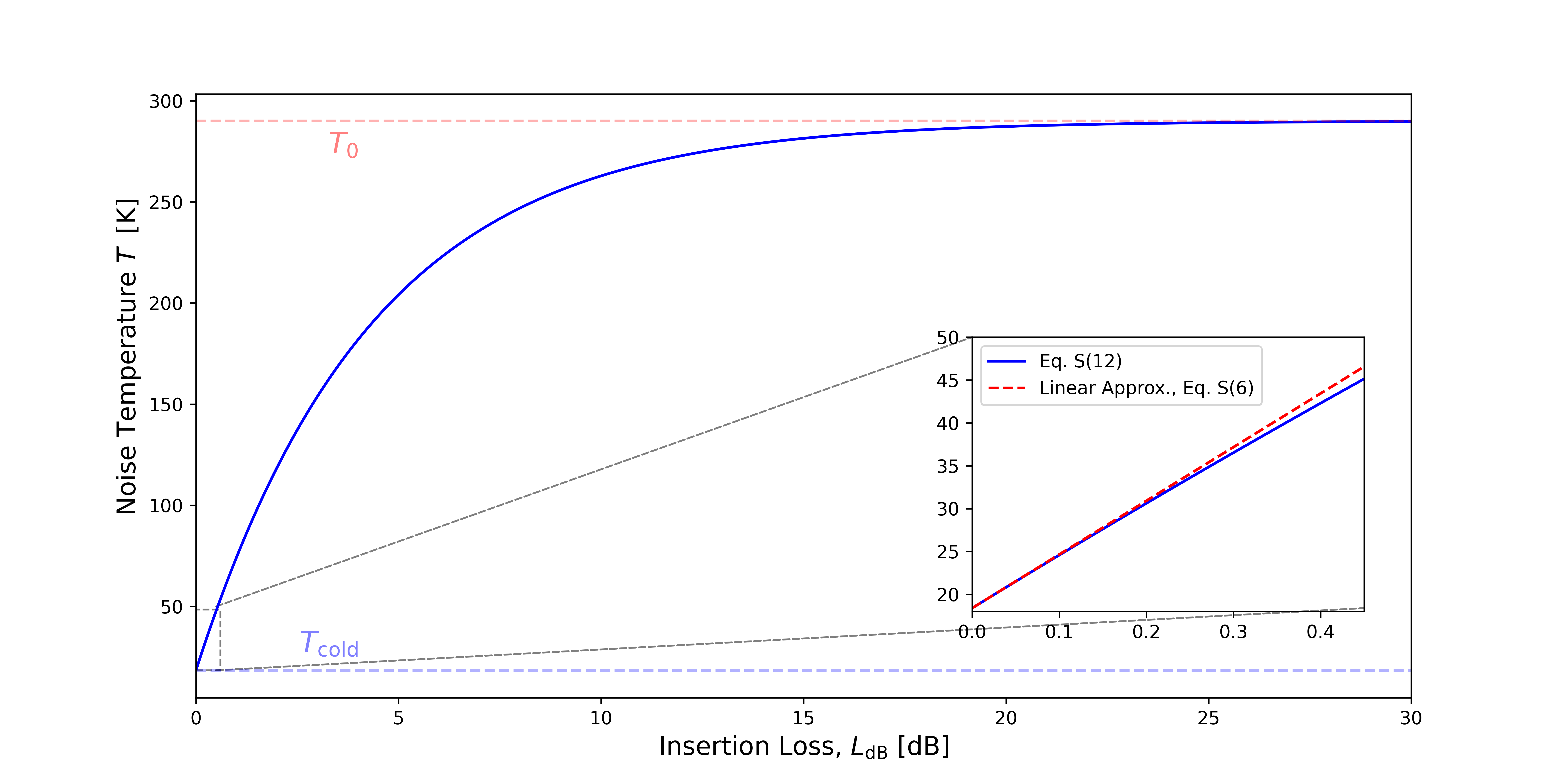
Figure 13: How, according to Eq. 14, the forward noise power (in units of absolute temperature $T$) at the far end of a lossy cable depends on the cable’s insertion loss $L_{\text{dB}}$. Here the cable is uniformly maintained at a temperature of $T_{\text{0}}=290$ K throughout its length and the near end of the cable is terminated and cooled by the an ACL whose noise temperature is $T_{\text{cold}}=18.2$ K (dashed cornflower-blue baseline)–corresponding to the input noise temperature of the Qorvo QPL9547EVB-01 LNA used experimentally. The zoomed-in area details how, when the insertion loss is less than 0.5 dB, equation Eq. 8 (red dashed line -“Linear Approx.”), i.e. the linear approximation provided by equation (8-2-5) in Siegman’s book [36], compares against the exact formula Eq. 14 (blue solid line).

A.3 NOISE ANALYSIS

Similar to the previous work by Wu et al. [1], we also adopt the “wave approach” (see Chapter 8 of Siegman [36]) to analyze the flow of noise power from the cavity into our homodyne receiver, as shown in Fig. 14. Equation S8 in the supplemental material of Wu et al.’s paper provides a formula for the factor, $\Delta P$ (in units of dB), by which measured noise power is reduced by mode cooling:

$$\Delta P^{\prime}=10\log_{10}\frac{{G_{\text{LNA}}[(T_{\text{min}}+T_{\text{mode}})(1-|\Gamma_{c}|^{2})+4T_{0}\frac{R_{\text{n}}}{Z_{0}}\frac{\lvert\Gamma_{\text{c}}-\Gamma_{\text{opt}}\rvert^{2}}{\lvert 1+\Gamma_{\text{opt}}\rvert^{2}}+T_{\text{image}}]+T_{\text{REC}}}}{{G_{\text{LNA}}[(T_{\text{min}}+T_{\text{mode}}^{0})(1-|\Gamma_{c}^{0}|^{2})+4T_{0}\frac{R_{\text{n}}}{Z_{\text{0}}}\frac{\lvert\Gamma_{c}^{0}-\Gamma_{\text{opt}}\rvert^{2}}{\lvert 1+\Gamma_{\text{opt}}\rvert^{2}}+T_{\text{image}}]+T_{\text{REC}}}},$$ (16)

However, this formula needs to be modified slightly for the following reasons: (i) Our current receiver is a homodyne, not a single-conversion superhet subject to additional image noise; one can thus set $T_{\text{image}}=0$. (ii) Even when monitoring (with the cooling LNA disconnected), the cavity mode is continuously cooled (albeit only slightly) by the receiver’s front-end LNA, connected to the cavity’s monitoring port via a lossy stub tuner and cable (substantially reducing the size of the cooling effect) –see main text. The ambient/reference mode temperature in the above formula, namely $T_{\text{mode}}^{0}$, should thus be set equal (again, see main text) to $T_{\text{mode}}^{\text{ambient}}\approx$ 255.2 K, somewhat less than 290 K. (iii) the ambient (reference) and post-cooled measurements are performed with the cavity under the same coupling conditions, namely with a single, critically-coupled monitoring port; the reflection amplitude off this port is always zero (during measurement of the noise power); thus, one can set $\Gamma_{c}=\Gamma_{c}^{0}=0$. These largely simplifying modifications lead to:

$$\Delta P=10\log_{10}\frac{{G_{\text{LNA}}[(T_{\text{min}}+T_{\text{mode}})+4T_{0}\frac{R_{\text{n}}}{Z_{0}}\frac{\lvert\Gamma_{\text{opt}}\rvert^{2}}{\lvert 1+\Gamma_{\text{opt}}\rvert^{2}}]+T_{\text{REC}}}}{{G_{\text{LNA}}[(T_{\text{min}}+T_{\text{mode}}^{\text{ambient}})+4T_{0}\frac{R_{\text{n}}}{Z_{\text{0}}}\frac{\lvert\Gamma_{\text{opt}}\rvert^{2}}{\lvert 1+\Gamma_{\text{opt}}\rvert^{2}}]+T_{\text{REC}}}},$$ (17)

where $T_{\text{mode}}$ is the pre-cooled mode temperature; $T_{\text{min}}$, $R_{\text{n}}$, $\Gamma_{\text{opt}}$ are the four noise parameters (being a complex number, $\Gamma_{\text{opt}}$ counts double) of the monitoring LNA, namely a Qorvo QPL9547EVB-01; the reference impedance $Z_{0}=50$ $\Omega$ throughout. The values assigned to these parameters, as shown in Table 1, have been interpolated to 1.45 GHz from measurements at straddling spot frequencies found in the manufacturer’s data sheet [49]. The noise temperature of the rest of the receiver, treated as a cascade of amplifiers, was calculated using the Friis formula and the amplifiers’ specified noise temperatures/figures [47]; see Table 1. The monitoring LNA’s gain, $G_{\text{LNA}}$, was measured using a VNA and found to be consistent with the QPL9547’s datasheet. The amplitude of the applied interrogating microwave tone was chosen to be sufficiently low that stimulated emission/absorption is very slow compared to the intrinsic spin dynamics of pentacene’s optically excited triplet state.

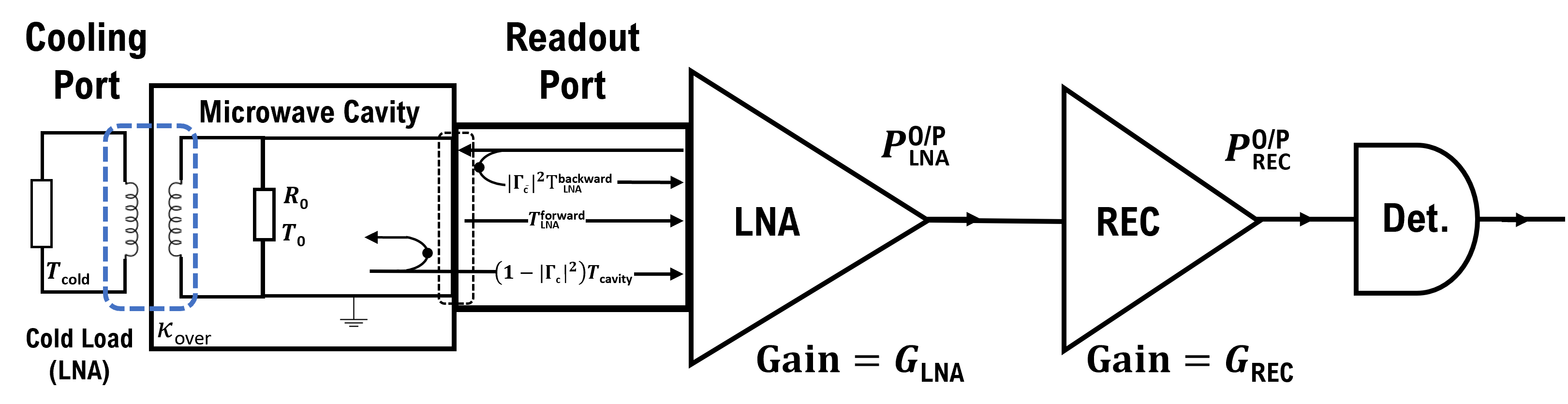
Figure 14: Anatomy of the signal path at the front end of the homodyne receiver, displaying the forward and backward noise powers between the LNA and microwave cavity.

Table 1: Values of parameters -entering the noise-reduction equation 17

Description of the Receiver	Symbol	Value (@ 1.4495 GHz)
Linear power gain of first LNA	$G_{\text{LNA}}$	166.0 $\pm 3.3$
Minimum noise figure of first LNA	$NF_{\text{min}}$	0.17*
Minimum noise temperature of first LNA	$T_{\text{min}}$	11.6 K*
Optimum source reflection coefficient	$\Gamma_{\text{opt}}$	(0.073+0.125)i*
Noise resistance of first LNA	$R_{\text{n}}$	2.00*
Noise temperature of the rest of the receiver	$T_{\text{REC}}$	36.1 K†
* interpolated from published datasheet [49]
$\dagger$ calculated using Friis formula[47]

Given the parameters appearing in Table 1 whose values compose the noise calibration of our tr-EPR spectrometer, the observed reduction in noise power provided by cavity precooling, as predicted by Eq. 17, depends on the value $T_{\text{mode}}$ in the numerator versus that of $T_{\text{mode}}^{\text{ambient}}$ in the denominator. The latter, corresponding to when the cavity’s $\textrm{TE}_{01\delta}$ mode is critically coupled to its monitoring LNA via a lossy stub tuner, should equal $(T_{0}+T_{\text{mon}})/2=255.4$ K, where $T_{\text{mon}}=10^{-\frac{L_{\text{dB,2}}}{10}}T_{\text{cold}}+(1-10^{-\frac{L_{\text{dB,2}}}{10}})T_{0}\approx 220.9$ K according to Eq. 14. Upon fixing the value of $T_{\text{mode}}^{\text{ambient}}$, Eq. 17 can be used to infer $T_{\text{mode}}$ from the experimentally observed reduction in noise power $\Delta P$. Using the data shown in Fig. 6(b), a rough estimate of $\Delta P$ can be arrived at from the difference in the spectral noise power, averaged from 5 to 10 MHz (so avoiding the 1/f noise prevalent below 1 MHz), between “pre-cooled” and “ambient” conditions. one obtains: $\Delta P_{\text{exp-EPR}}=-3.7\pm 1$ dB. Since this estimate of $\Delta P$ has greater uncertainty than that derived directly from monitoring the pre-cooling in the time domain, namely $\Delta P_{\text{exp-Cool}}$, it is not further used.

The mode temperature $T_{\text{mode}}$ can be separately determined by Eq.15; it depends on the (presumed identical) noise temperature of the two LNAs, $T_{\text{cold}}$, the coupling factor of the over-coupling loop $\kappa_{\text{over}}$, and the insertion losses of the RF switch $L_{\text{dB, 1}}$ and the monitoring LNA’s connection to the cavity line $L_{\text{dB,2}}$. One arrives at

$$T_{\text{mode, EPR}}=\frac{T_{\text{0}}+\kappa_{\text{over}}[(1-\frac{L_{\text{dB,1}}}{4.34})T_{\text{cold}}+\frac{L_{\text{dB,1}}}{4.34}T_{0}]+[10^{-\frac{L_{\text{dB,2}}}{10}}T_{\text{cold}}+(1-10^{-\frac{L_{\text{dB,2}}}{10}})T_{0}]}{2+\kappa_{\text{over}}}\approx 108.1\pm 5~{}\text{K}.$$ (18)

The values of $L_{\text{dB,1}}$ and $L_{\text{dB,2}}$ at 1.4495 GHz were measured using our VNA (HP-8753C) to be $0.19\pm 0.01$ dB and $6.05\pm 0.01$ dB, respectively. The coupling factor between the cavity and the cold load was characterized by the method(s) of Kajfez and Hwan [34] using the same VNA; we obtained $\kappa_{\text{over}}=3.8\pm 0.3$. The value of $T_{\text{cold}}$ is calculated to be $18.4\pm 0.5$ K based on the definition of noise parameters[46], utilizing the parameters listed in Table 1. $T_{0}$ represents room temperature, set at $290$ K. The uncertainty of $T_{\text{mode, EPR}}$ shown in Eq. 18 is calculated by applying Pythagoras’ theorem to error propagation. Based on this result, we can use Eq 17 to obtain $\Delta P_{\text{sim}}=-3.5\pm 0.2$ dB.

The depth of mode cooling was also estimated by fitting a bi-exponential function to the increase in measured noise power upon switching out the cooling LNA, as shown in Fig. 4 in the main paper. The best-fit curve, along with a standard error band, is depicted in Fig. 15; this determined $\Delta P_{\text{exp-Cool}}=-3.5\pm 0.4$ dB, agreeing both with our simulated $\Delta P_{\text{sim}}$ and our analysis using the noise spectrum from tr-EPR data, namely $\Delta P_{\text{exp-EPR}}$ as shown in Fig. 6(b) of the main text. Our estimates are summarized in Table 2.

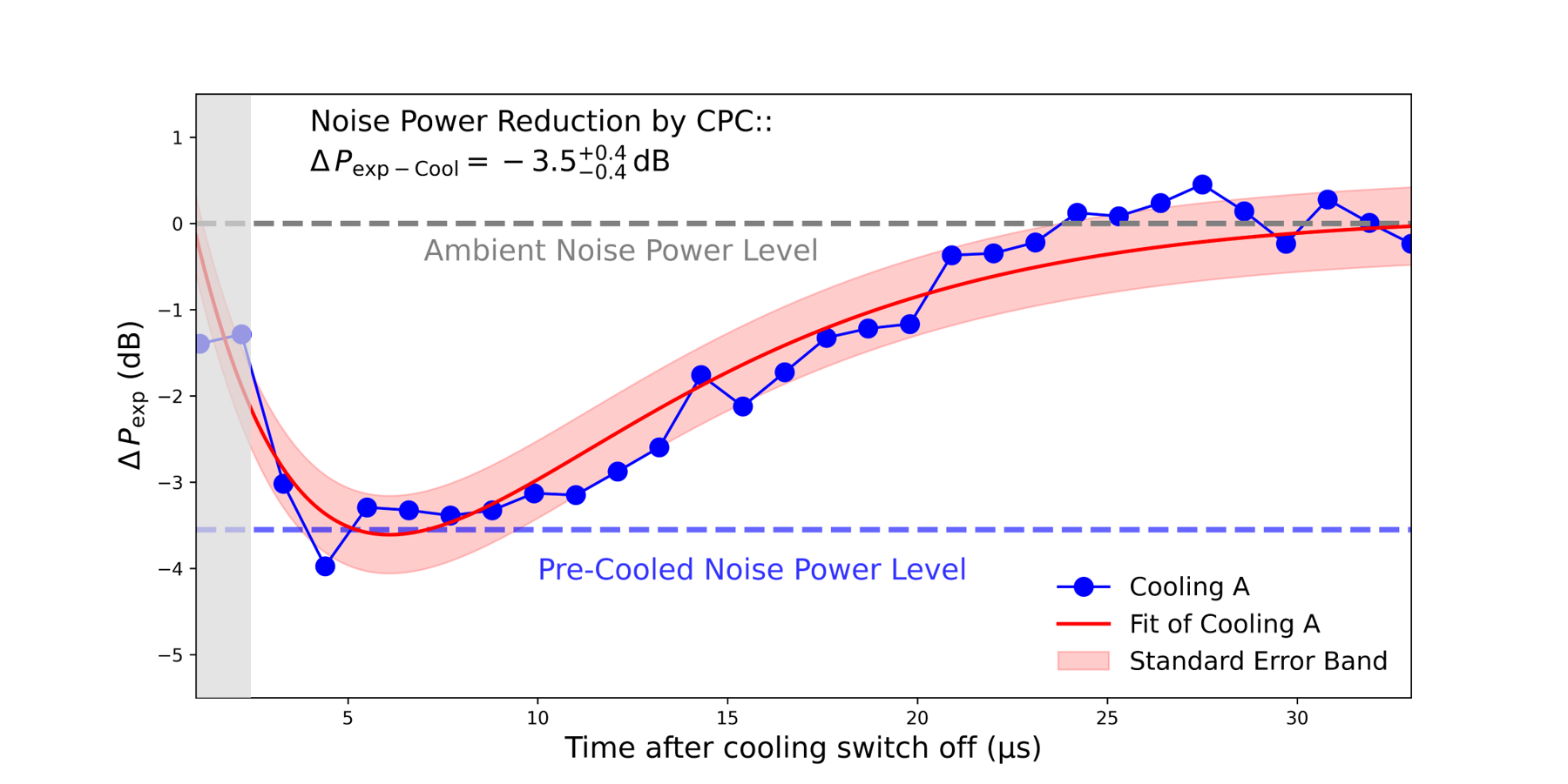
Figure 15: Error analysis and fitting of the experimental warming-up signal as presented in Fig. 4 of the main paper. The grey area represents the period when the double-throw switch is still transitioning to connect the over-coupled port to an “open” load, disconnecting the ACL from the resonator; this takes around $t_{\text{switch}}=2$ $\mu$s. Each blue dot plots $\Delta P_{\text{exp}}=10\log_{10}(<V^{2}_{\text{cold}}>/<V^{2}_{\text{ambient}}>)$ in units of dB[48], where $<V^{2}_{\text{cold}}>$ is the mean-squared received noise voltage averaged over ten consecutive data points, spaced 100 ns apart, spanning one microsecond; $<V^{2}_{\text{ambient}}>$ is the equivalent mean-squared noise voltage under ambient conditions (based on an adjoining sample spanning several hundred microseconds). The solid red line, along with its surrounding salmon pink standard error band, was obtained by least-squares fitting a bi-exponential to the evolution of $\Delta P_{\text{exp}}$ excluding the initial switching period. The longer of the two decay constants was determined to be $\tau_{\text{warm up}}^{\text{exp.}}\approx 9\pm 1\mu$s.

Table 2: Simulated and experimentally-inferred depth of cooling

method:	Simulation	Direct monitoring	EPR data analysis
		(time-domain)	(frequency-domain)
label:	sim	exp-Cool	exp-EPR
Noise-Power Reduction ($\Delta$ P) in dB:	3.5	3.5	3.7
Standard Deviation of $\Delta$ P:	$\pm$ 0.2	$\pm$ 0.4	$\pm$ 1.0

References

- Wu et al. [2021] H. Wu, S. Mirkhanov, W. Ng, and M. Oxborrow, Bench-top cooling of a microwave mode using an optically pumped spin refrigerator, Phys. Rev. Lett. 127, 053604 (2021).
- Ng et al. [2021] W. Ng, H. Wu, and M. Oxborrow, Quasi-continuous cooling of a microwave mode on a benchtop using hyperpolarized nv- diamond, Appl. Phys. Lett. 119, 234001 (2021).
- Fahey et al. [2023] D. P. Fahey, K. Jacobs, M. J. Turner, H. Choi, J. E. Hoffman, D. Englund, and M. E. Trusheim, Steady-state microwave mode cooling with a diamond n-v ensemble, Phys. Rev. Appl. 20 , 014033 (2023).
- Wang et al. [2024] H. Wang, K. L. Tiwari, K. Jacobs, M. Judy, X. Zhang, D. R. Englund, and M. E. Trusheim, A spin-refrigerated cavity quantum electrodynamic sensor, arXiv quant-pph (16th April 2024).
- Day et al. [2024] T. Day, M. Isarov, W. J. Pappas, B. C. Johnson, H. Abe, T. Ohshima, D. R. McCamey, A. Laucht, and J. J. Pla, A room-temperature solid-state maser amplifier, arXiv:2405.07486v1 [quant-ph] (13 May 2024).
- Breeze et al. [2015] J. Breeze, K.-J. Tan, B. Richards, J. Sathian, M. Oxborrow, and N. N. Alford, Enhanced magnetic purcell effect in room-temperature masers, Nature Comm. 6, 6215 (2015).
- Fleury et al. [2023] R. Fleury, R. Xiang, P. Bugnon, and M. Khatibi, All-metallic magnetic purcell enhancement in a thermally stable room-temperature maser, preprint: https://doi.org/10.21203/rs.3.rs-3536841/v1 (2023).
- Friis [1944] H. T. Friis, Noise figures of radio receivers, Proc. IRE 32, 419 (July 1944).
- Šimėnas et al. [2021] M. Šimėnas, J. O’Sullivan, C. W. Zollitsch, O. Kennedy, M. Seif-Eddine, I. Ritsch, M. Hülsmann, M. Qi, A. Godt, M. M. Roessler, et al., A sensitivity leap for x-band epr using a probehead with a cryogenic preamplifier, J. Mag. Res. 322, 106876 (2021).
- Giordmaine et al. [1959] J. Giordmaine, L. Alsop, C. Mayer, and C. Townes, A maser amplifier for radio astronomy at x-band, Proc. IRE 47, 1062 (1959).
- Clauss and Shell [2008] R. C. Clauss and J. S. Shell, Chapter 3: Ruby masers, in Low-Noise Systems in the Deep Space Network, edited by M. S. Reid (JPL, NASA, 2008) pp. 95–158.
- Collier et al. [1968] R. J. Collier, M. A. Collins, and D. G. Moss, An x-band electron spin resonance spectrometer with a ruby maser preamplifier, J. Phys. E: Sci. Instr. 1, 607 (1968).
- Narkowicz et al. [2013] R. Narkowicz, H. Ogata, E. Reijerse, and D. Suter, A cryogenic receiver for epr, J. Mag. Res. 237, 79 (2013).
- Kalendra et al. [2023] V. Kalendra, J. Turčak, J. Banys, J. J. L. Morton, and M. Šime, X- and q-band epr with cryogenic amplifiers independent of sample temperature, J. Mag. Res. 343, 107356 (2023).
- Pfenninger et al. [1995] S. Pfenninger, W. Froncisz, and J. S. Hyde, Noise analysis of epr spectrometers with cryogenic microwave preamplifiers, J. Mag. Res., Series A 113, 32 (1995).
- Townes [1960] C. Townes, Sensitivity of microwave spectrometers using maser techniques, Phys. Rev. Lett. 5, 428 (1960).
- Mollier et al. [1973] J. Mollier, J. Hardin, and J. Uebersfeld, Theoretical and experimental sensitivities of esr spectrometers using maser techniques, Rev. Sci. Instrum. 44, 1763 (1973).
- Poole and Farach [2019] C. P. Poole and H. A. Farach, Electron spin resonance, in Handbook of Spectroscopy (CRC Press, 2019) pp. 217–314.
- Hill and Richards [1968] H. Hill and R. Richards, Limits of measurement in magnetic resonance, J. Phys. E: Sci. Instr. 1, 977 (1968).
- Rinard et al. [1999] G. A. Rinard, R. W. Quine, J. R. Harbridge, R. Song, G. R. Eaton, and S. S. Eaton, Frequency dependence of epr signal-to-noise, J. Mag. Res. 140, 218 (1999).
- Weinreb et al. [1982] S. Weinreb, D. L. Fenstermacher, and R. W. Harris, Ultra-low-noise 1.2-to 1.7-ghz cooled gaasfet amplifiers, IEEE Trans. Microwave Theory and Tech. 30, 849 (1982).
- Pospieszalski [2024] M. Pospieszalski, Extremely low-noise amplification with cryogenic fets and hfets: 1970-2004, in IEEE Microwave Magazine, Vol. 6 (IEEE, 2024) pp. 62–75.
- Wu et al. [2020a] H. Wu, S. Mirkhanov, W. Ng, K.-C. Chen, Y. Xiong, and M. Oxborrow, Invasive optical pumping for room-temperature masers, time-resolved epr, triplet-dnp, and quantum engines exploiting strong coupling, Optics Express 28, 29691 (2020a).
- Blank et al. [2023] A. Blank, A. Sherman, B. Koren, and O. Zgadzai, An anti-maser for mode cooling of a microwave cavity, J. Appl. Phys. 134, 214401 (2023).
- Gervasi et al. [1995] M. Gervasi, G. Bonelli, G. Sironi, F. Cavaliere, A. Passerini, and S. Casani, An absolute cryogenic calibration source for a 2.5 ghz radiometer, Rev. Sci. Instrum. 66, 4798 (1995).
- Albanese et al. [2020] B. Albanese, S. Probst, V. Ranjan, C. W. Zollitsch, M. Pechal, A. Wallraff, J. J. Morton, D. Vion, D. Esteve, E. Flurin, et al., Radiative cooling of a spin ensemble, Nature Physics 16, 751 (2020).
- Wang et al. [2021] Z. Wang, M. Xu, X. Han, W. Fu, S. Puri, S. M. Girvin, H. X. Tang, S. Shankar, and M. H. Devoret, Quantum microwave radiometry with a superconducting qubit, Phys. Rev. Lett. 26, 180501 (2021).
- Frater and Williams [1981] R. H. Frater and D. R. Williams, An active "cold" noise source, IEEE Trans. Microwave Theory and Tech. 29, 344 (1981).
- Forward and Terry [2010] R. Forward and C. Terry, Electronically cold microwave artificial resistors, IEEE Trans. Microwave Theory and Tech. 31, 45 (2010).
- Leynia de la Jarrige et al. [2010] E. Leynia de la Jarrige, L. Escotte, E. Gonneau, and J.-M. Goutele, Sige hbt-based active cold load for radiometer calibration, IEEE Microwave and Wireless Components Letters 20, 238 (2010).
- Weissbrodt [2017] E. Weissbrodt, Active Electronic Loads for Radiometric Calibration, Ph.D. thesis, University of Stuttgart (2017).
- Shou et al. [2015] N. Shou, S. S. Søbjærg, J. Balling, and S. Kristensen, A second generation l-band digital radiometer for sea salinity campaigns, Proc. IEEE Geosc. Remote Sens. Symposium (IGARSS), Milan , 4742 (2015).
- Oxborrow [2007] M. Oxborrow, Traceable 2-d finite-element simulation of the whispering-gallery modes of axisymmetric electromagnetic resonators, IEEE Trans. Microwave Theory and Tech. 55, 1209 (2007).
- Kajfez and Hwan [1984] D. Kajfez and E. J. Hwan, Q-factor measurement with network analyzer, IEEE Trans. Microwave Theory and Tech. 32, 666 (1984).
- Chua and Mirshekar-Syahkal [2003] L. H. Chua and D. Mirshekar-Syahkal, Accurate and direct characterization of high-q microwave resonators using one-port measurement, IEEE Trans. Microwave Theory and Tech. 51, 978 (2003).
- Siegman [1964] A. E. Siegman, Microwave solid-state masers (McGraw-Hill, 1964).
- Aspelmeyer et al. [2014] M. Aspelmeyer, T. J. Kippenberg, and F. Marquardt, Cavity optomechanics, Rev. Mod. Phys. 86, 1391 (2014).
- Hewlett Packard / Agilent [1983] Hewlett Packard / Agilent, Application Note 57-1: Fundamentals of RF and Microwave Noise Figure Measurements, The Hewlett Packard Archive (revised July 1983).
- Raimond et al. [1982] J. Raimond, P. Goy, M. Gross, C. Fabre, and S. Haroche, Collective absorption of blackbody radiation by rydberg atoms in a cavity: an experiment on bose statistics and brownian motion, Phys. Rev. Lett. 49, 117 (1982).
- Wu et al. [2020b] H. Wu, X. Xie, W. Ng, S. Mehanna, Y. Li, M. Attwood, and M. Oxborrow, Room-temperature quasi-continuous-wave pentacene maser pumped by an invasive ce:yag luminescent concentrator, Phys. Rev. Applied 14, 064017 (2020b).
- Ardizzi et al. [2022] A. J. Ardizzi, A. Y. Choi, B. Gabritchidze, J. Kooi, K. A. Cleary, A. C. Readhead, and A. J. Minnich, Self-heating of cryogenic high electron-mobility transistor amplifiers and the limits of microwave noise performance, J. Appl. Phys. 132, 084501 (2022).
- Zeng et al. [2024] Y. Zeng, J. Stenarson, P. Sobis, N. Wadefalk, and J. Grahn, Sub-mw cryogenic inp hemt lna for qubit readout, IEEE Trans. Microwave Theory and Tech. 72, 1606 (2024).
- Cakaj et al. [2011] S. Cakaj, B. Kamo, I. Enesi, and O. Shurdi, Antenna noise temperature for low earth orbiting satellite ground stations at l and s band, Europe 5, 6 (2011).
- Hyde [2005] J. S. Hyde, Trends in epr technology, in Biomedical EPR, Part B: Methodology, Instrumentation, and Dynamics (Springer, 2005) pp. 409–428.
- Henschel et al. [2010] K. Henschel, J. Majer, J. Schmiedmayer, and H. Ritsch, Cavity qed with an ultracold ensemble on a chip: Prospects for strong magnetic coupling at finite temperatures, Phys. Rev. A 82, 033810 (2010).
- Escotte et al. [1993] L. Escotte, R. Plana, and J. Graffeuil, Evaluation of noise parameter extraction methods, IEEE transactions on microwave theory and techniques 41, 382 (1993).
- Kraus [1986] J. Kraus, D.: Radio astronomy (cygnus-quasar books, powell (1986).
- Sung et al. [2003] J.-J. Sung, G.-S. Kang, and S. Kim, A transient noise model for frequency-dependent noise sources, IEEE Transactions on Computer-Aided Design of Integrated Circuits and Systems 22, 1097 (2003).
- QPL [2023] datasheet: QPL9547, 0.1 - 6 GHz Ultra Low-Noise LNA, Rev. D, Qorvo (2023).
- Wu et al. [2019] H. Wu, W. Ng, S. Mirkhanov, A. Amirzhan, S. Nitnara, and M. Oxborrow, Unraveling the room-temperature spin dynamics of photoexcited pentacene in its lowest triplet state at zero field, The Journal of Physical Chemistry C 123, 24275 (2019).
- Hassan and Anwar [2010] U. Hassan and M. S. Anwar, Reducing noise by repetition: introduction to signal averaging, European Journal of Physics 31, 453 (2010).
- Dordević et al. [2015] V. Dordević, Z. Marinković, G. Crupi, O. Pronić-Rančić, V. Marković, and A. Caddemi, Wave approach for noise modeling of gallium nitride high electron-mobility transistors, International Journal of Numerical Modelling: Electronic Networks, Devices and Fields 30, e2138 (2015).
*