Fast fitting of phylogenetic mixed effects models

Abstract

Mixed effects models are among the most commonly used statistical methods for the exploration of multispecies data. In recent years, also Joint Species Distribution Models and Generalized Linear Latent Variale Models have gained in popularity when the goal is to incorporate residual covariation between species that cannot be explained due to measured environmental covariates. Few software implementations of such models exist that can additionally incorporate phylogenetic information, and those that exist tend to utilize Markov chain Monte Carlo methods for estimation, so that model fitting takes a long time. In this article we develop new methods for quickly and flexibly fitting phylogenetic mixed models, potentially incorporating residual covariation between species using latent variables, with the possibility to estimate the strength of phylogenetic structuring in species responses per environmental covariate, and while incorporating correlation between different covariate effects. By combining Variational approximations with a reduced rank matrix normal covariance structure, Nearest Neighbours Gaussian Processes, and parallel computation, phylogenetic mixed models can be fitted much more quickly than the current state-of-the-art. Two simulation studies demonstrate that the proposed combination of approximations is not only fast, but also enjoys high accuracy. Finally, we demonstrate use of the method with a real world dataset of wood-decaying fungi.

Introduction

The exploration of species co-occurrence patterns is at the core of contemporary community ecology. Recent years have seen a push in methods that better facilitate ecologists to understand which species co-occur, and why they co-occur (A. R. Ives and Helmus 2011; Braga et al. 2018). Some species co-occur because they thrive in similar environments, which may be due to similar characteristics in terms of functional traits. Species that share evolutionary history often share such physical characteristics, and consequently hypotheses exist that describe the co-occurrence of closely related species (Pagel 1999).

Data on ecological communities is increasingly analysed with multivariate statistical models. Most notably, Joint Species Distribution Models (JSDMs, Pollock et al. 2014) are now frequently applied for the analysis of binary data of multiple species. Such models represent co-occurrence patterns by incorporating residual covariation that cannot be explained due to the measured environment. Generalized Linear Latent Variable Models (GLLVMs, Warton et al. 2015) are a modeling framework that uses latent variables to represent unmeasured drivers of species co-occurrence patterns. GLLVMs have been presented as a model-based method for ordination (Hui et al. 2015; van der Veen et al. 2023), but are also a computationally efficient method for implementing JSDMs.

GLLVMs tend to be challenging to fit for species that do not have many observations. Such species may be referred to as “rare” by ecologists, but we here generally refer to species that have few observations, such as due to insufficient sampling. In order to ameliorate such issues with few data points, and to incorporate the relatedness of species into the analysis of species co-occurrence patterns, JSDMs have been developed that phylogenetically structure species responses to the environment. In such models, species that are more closely related can be predicted to co-occur (Ovaskainen et al. 2017). This has the benefit of “sharing” information across related species, so that species may more accurately be placed in the environment. In fact, with such models it is possible to predict the environmental preferences of extinct species for which no response observations area available at all, by utilizing phylogenetic information.

Three notable software implementations for such phylogenetic random effects models are the Hmsc (Tikhonov et al. 2024), MCMCglmm (Hadfield 2010), and phyr (A. Ives et al. 2020) R-packages. Unfortunately, these software implementations are either slow because they use Markov chain Monte Carlo for estimation (Hmsc and MCMCglmm) or are limited in their functionality otherwise (e.g., phyr supports few datatypes). Since phylogenetic information and community data of species is becoming more readily available thanks to various openscience initiatives, this motivates development of better, and faster, software implementations of community models that incorporate phylogenetic information.

In this article, we present a new statistical approach for fast fitting of phylogenetic random effects models for community ecological data as part of the gllvm R-package. The proposed modeling framework can alternatively be used for when response data are functional traits, or data on individuals (with a pedigree instead of a phylogeny as in MCMCglmm), but we choose to focus here on community data. The package supports a range of datatypes commonly found in community ecological, such as for counts of individuals (Poisson and negative-binomial, potentially zero-inflated), cover classes (ordinal), percentage cover (beta models potentially with zeros or ones, see Korhonen et al. (2024)), and biomass (Tweedie, see Korhonen et al. (2021) and Niku et al. (2017)). Niku et al. (2021) implemented species-specific random effects as part of the fourth corner latent variable model. Phylogenetic information can facilitates better estimation of species responses to the environment, while latent variables can still be included to account for residual covariation. 1) Phylogenetically structuring the random effects, 2) for which we provide functionality to determine strength of the phylogenetic signal per covariate, and 3) facilitate specification of correlation between random effects using the user-friendly lme4 formula interface (Bates et al. 2015)

Using a combination of methodological developments we can fit the models much more quickly than existing software implementations for Phylogenetically structured random effect models. Variational Approximations (VA, Ormerod and Wand 2010) helps to retrieve a closed form approximation to the likelihood, which we combine with a matrix normal covariance structure for the variational distribution, as well as a reduced-rank approximation to further speed it up. Nearest Neighbour Gaussian processes (NNGPs, Finley et al. 2019) facilitate even quicker computation by forming a sparse approximation to the inverse of the phylogenetic covariance matrix. Finally, fitting the models in parallel via the TMB R-package (Kristensen et al. 2015) further reduces computation time.

With extensive simulations we show that the proposed combination of four approximations still allows us to accurately retrieve the model parameters, and that it tends to be faster than application of the Laplace approximation (e.g., as in the phyr R-package). Using data from Abrego et al. (2022a) we demonstrate use of the model on a real dataset.

Model formulation

In this section we present and explain the phylogenetic random effects model, and in the next section we discuss estimation of the parameters.

Let Y represent a multivariate dataset with rows $i=1\ldots n$ that represent the sites at which an ecological community has been surveyed, and the columns $j=1\ldots m$ represent the species found. $\textbf{X}=\begin{bmatrix}\textbf{x}_{1},\textbf{x}_{2},\ldots\textbf{x}_{k}\end{bmatrix}^{\top}$ is a set of $k=1\ldots p$ covariates with an associated $p\times m$ coefficient matrix $\boldsymbol{\beta}$ for the environment that has been observed at each site, which also includes an intercept column. Covariates can be categorical to represent species-specific intercepts under different conditions, or numerical to represent species-specific responses to the environment, i.e., as slope parameters. As in generalised linear models (GLMs) a link function $\text{g}(\cdot)$ connects the linear predictor $\boldsymbol{\eta}$ to the mean of the conditional distribution assumed for observation $y_{ij}$, so that the model generically is

$$\text{g}\{\mathams{E}(\textbf{Y}|\boldsymbol{\beta})=\textbf{X}\boldsymbol{\beta}\}.$$ (1)

where X includes an a column of ones for the intercepts. This model can additionally be extended with functional traits as in the fourth corner latent variable model developed in Niku et al. (2021), by hierarchically modeling the species responses:

$$\boldsymbol{\beta}=\textbf{1}^{\top}\boldsymbol{\beta}_{x}+\textbf{T}\boldsymbol{B}_{tx}+\boldsymbol{\beta}_{\epsilon},$$ (2)

where 1 is a $m$-sized vector of ones, $\boldsymbol{\beta}_{x}$ is a $K$-sized vector of community mean responses to the covariates, T is a $m\times t$ matrix of observed functional traits, $\boldsymbol{B}_{tx}$ is a $t\times p$ matrix of fourth corner coefficients that represent environment-trait interactions, and $\boldsymbol{\beta}_{\epsilon}$ is a matrix of $p\times m$ species-specific random effects for the covariates that model species-specific deviations from the community mean response. The species responses $\boldsymbol{\beta}$ can be thought of as latent traits, which are modeled with observed trait covariates. Excluding the trait covariates simplifies the model to, equivalent to assuming that species responses to the environment are not structured by observed traits.

Let C denote the phylogenetic correlation matrix, and $\boldsymbol{\mu}_{k}$ generically the mean of species environmental responses (with or without traits). To phylogenetically structure the random effects we could assume $\boldsymbol{\beta}_{k}\sim\mathcal{N}(\boldsymbol{\mu}_{k},\sigma_{k}^{2}\textbf{C})$, so that $\sigma_{k}^{2}$ represents the rate of evolution, which determines the variance of the random effect. However, unless there is a phylogenetic signal this model is quite restrictive, so phylogenetic random effects models (e.g., as in the phyr R-package) are usually formulated with a second set of random effects that are independent for all species $\boldsymbol{\beta}_{2k}$ with variance $\sigma_{2k}^{2}$. Since $\boldsymbol{\beta}_{1k}$ and $\boldsymbol{\beta}_{2k}$ are independent, we define $\boldsymbol{\beta}_{k}=\boldsymbol{\beta}_{1k}+\boldsymbol{\beta}_{2k}\sim\mathcal{N}[\textbf{0},\sigma^{2}_{k}\{\textbf{C}\rho_{k}+(1-\rho_{k})\textbf{I}_{m}\}]$ where $\rho_{k}=\frac{\sigma_{1k}^{2}}{\sigma^{2}_{1k}+\sigma_{2k}^{2}}$ is the phylogenetic signal parameter per covariate (equivalent to Pagel’s $\lambda$, see Pagel (1999) and Pearse, Davies, and Wolkovich (2023)), and $\sigma^{2}_{k}=\sigma^{2}_{1}+\sigma^{2}_{2}$ is the variance of the sum of the two terms. Consequently, the variances of the original two terms can be retrieved from this alternative model formulation by nothing that $\sigma^{2}_{1k}=\rho_{k}\sigma_{k}^{2}$ and $\sigma^{2}_{2k}=(1-\rho_{k})\sigma^{2}_{k}$. This formulation has the benefit of only including one set of random effects that need to be integrated out of the likelihood (which is usually computationally intensive for many random effects), but the downside that it requires explicit inversion of the covariance matrix for species at each iteration during model fitting (which tends to be computationally intensive for many species).

Covariances between the random effects of different covariates $\boldsymbol{\Sigma}_{r}$, i.e., for the rows of $\boldsymbol{\beta}_{\epsilon}$ can be introduced by instead defining the distribution of the random effects over all species and covariates simultaneously. Let $\textbf{L}_{k}(\boldsymbol{\Sigma}_{k})$ denote the lower cholesky factor of $\boldsymbol{\Sigma}_{k}$, so that instead we parameterize the covariance over the random effects for all species and covariates as

$$\text{vec}(\boldsymbol{\beta}_{\epsilon}^{\top})\sim\mathcal{N}[\textbf{0},\begin{Bmatrix}\textbf{L}(\boldsymbol{\Sigma}_{1})&&&\\ &\textbf{L}(\boldsymbol{\Sigma}_{2})&&\\ &&\ddots&&\\ &&&\textbf{L}(\boldsymbol{\Sigma}_{p})\end{Bmatrix}\biggl{\{}\boldsymbol{\Sigma}_{r}\otimes\textbf{I}_{m}\biggr{\}}\begin{Bmatrix}\textbf{L}(\boldsymbol{\Sigma}_{1})^{\top}&&&\\ &\textbf{L}(\boldsymbol{\Sigma}_{2})^{\top}&&\\ &&\ddots&&\\ &&&\textbf{L}(\boldsymbol{\Sigma}_{p})^{\top}\end{Bmatrix}],$$ (3)

where $\boldsymbol{\Sigma}_{mp}=\textbf{C}\rho_{p}+(1-\rho_{p})\textbf{I}_{m}$. If instead we assume $\rho_{k}=\rho$, i.e., that the phylogenetic signal is the same for all covariates, equation (3) reduces to equation (4) of Ovaskainen et al. (2017) or equation (11.1-2) of de Villemereuil and Nakagawa (2014), i.e., $\text{vec}(\boldsymbol{\beta}_{\epsilon})\sim\mathcal{N}(\textbf{0},\boldsymbol{\Sigma}\otimes\boldsymbol{\Sigma}_{r})$. In this formulation, $\boldsymbol{\Sigma}_{r}$ controls correlation between covariate effects of the same species, and together with the phylogenetic signal parameters also the correlation between covariate effects of different species. These off-diagonal blocks in the covariance matrix are by extension formulated as an lu decomposition and take the form $\textbf{L}_{k}(\boldsymbol{\Sigma}_{k})\textbf{L}_{l}(\boldsymbol{\Sigma}_{l})^{\top}\Sigma_{kl}$. The lower triangular matrix of this lu decomposition is $\textbf{L}_{k}(\boldsymbol{\Sigma}_{k})\text{Diag}[\text{diag}\{\textbf{L}_{k}(\boldsymbol{\Sigma}_{k})\}^{-1}$, where $\text{Diag}(\cdot)$ constructs a diagonal matrix from a vector and $\text{diag}(\cdot)$ extracts the diagonal of a matrix. The associated upper triangular matrix is then $\text{Diag}[\text{diag}\{\textbf{L}_{k}(\boldsymbol{\Sigma}_{k})\}]\textbf{L}_{l}(\boldsymbol{\Sigma}_{l})^{\top}\Sigma_{kl}$.

For brevity, let $\text{bdiag}\{\textbf{L}(\boldsymbol{\Sigma}_{k})\}$ represent the blockdiagonal matrix of lower cholesky factors as in equation (3). Consequently, the matrix of species associations at sites $i$ and $l$ due to the phylogenetic random effects model with multiple signal parameters is:

$$\boldsymbol{\Sigma}_{spp}=(\textbf{x}_{i}^{\top}\otimes\textbf{I}_{m})\text{bdiag}\{\textbf{L}(\boldsymbol{\Sigma}_{k})\}(\boldsymbol{\Sigma}_{r}\otimes\textbf{I}_{m})\text{bdiag}\{\textbf{L}(\boldsymbol{\Sigma}_{k})^{\top}\}(\textbf{x}_{i}\otimes\textbf{I}_{m})$$ (4)

The model in equation (1) can be extended in various ways, for example by incorporating unconstrained latent variables as in Niku et al. (2021), or constrained or informed latent variables (van der Veen et al. 2023), potentially with a quadratic response model (van der Veen et al. 2021), with random site effects to account for pseudoreplication (as demonstrated in the following case study) or spatial autocorrelation, or with additional fixed effects, but we have omitted those here for brevity.

Similarly, in its present form the model only incorporates positive species associations. It is possible to adjust the model to additionally incorporate negative species assocations, but we consider such an implementation as a future avenue for research (see also appendix S1).

Parameter estimation

In this section we elaborate on the four approximations that are implemented to quickly fit the phylogenetic random effect models. We evaluate the accuracy of these stacked approximations using simulation studies in the following section.

Formulating the model in terms of a single set of random effects $\boldsymbol{\beta}_{\epsilon}\sim\mathcal{N}(\textbf{0},\boldsymbol{\Sigma})$, with a vector $\Theta$ of all other parameters in the model (such as dispersion parameters for a Tweedie or negative binomial distribution), we have the following marginal log-likelihood function:

$$\mathcal{L}(\boldsymbol{\Theta})=\sum\limits_{j=1}^{m}\log\biggl{[}\int\prod\limits_{i=1}^{n}f\biggl{(}y_{ij}|\boldsymbol{\beta}_{\epsilon}\biggr{)}\mathcal{N}\biggl{\{}\text{vec}\biggl{(}\boldsymbol{\beta}_{\epsilon}\biggr{)};\boldsymbol{\Sigma}\biggr{\}}d\boldsymbol{\beta}_{\epsilon}\biggr{]}.$$ (5)

To efficiently retrieve a closed-form approximation to the log-likelihood in equation (5), we use VA (Hui et al. 2017). VA introduces hyperparameters (“variational parameters”) that need to be optimised in order to improve the approximation (tightening the lower bound). With many species and random effects this can significantly slow down model fitting. Other methods for fitting generalized mixed-effects models, such as the Laplace approximation, suffer from similar issues with high dimensions. The Laplace approximation requires evaluating the matrix of second derivatives of the joint likelihood for the random effects and the data, which also significantly slows down for a large number of (correlated) random effects. VA has the benefit of allowing for a second approximation by introducing a more simple structure for the VA covariance matrix, so that the size of the optimisation problem is reduced significantly for quicker model fitting.

Various VA covariance structures are possible to formulate, but some require unrealistic assumptions (such as independence of species or random effects), or have a considerably higher number of variational parameters (e.g., as in an unstructured covariance matrix), so that they require significantly longer computational times. In one of the most reduced scenarios, we assume the variational distribution for the random effects to follow a matrix normal distribution, i.e., $q(\boldsymbol{\beta}_{\epsilon})=\mathcal{MN}(\textbf{a},\textbf{A}_{r},\textbf{A}_{m})$ with $\textbf{A}_{r}$ a $p\times p$ VA covariance matrix and $\textbf{A}_{m}$ a $m\times m$ VA covariance matrix. Some different formulations are provided in the supplementary information (appendix S2) and implemented in the gllvm R-package. For the remainder of this article, we limit ourselves to application of the matrix normal case. We show in the simulations below that the choice of a matrix normal VA distribution still enjoys high accuracy, despite its relative inflexibility.

With this choice of a matrix normal covariance strucutre, VA can still be slow due to the potentially large number of variational parameters in $\textbf{A}_{m}$. The number of variational parameters in this matrix grows quadratically in the number of species. To ensure better scaling, and quick computation also with many species, we employ a third approximation by representing the off-diagonal entries of $\textbf{A}_{m}$ in a reduced-rank fashion so that $d<<m$, i.e., $\textbf{A}_{m}=\textbf{A}_{d}\textbf{A}_{d}^{\top}+\textbf{A}_{m-d}$ where $\textbf{A}_{d}$ is a $m\times d$ lower triangular matrix with positive diagonal entries, and $\textbf{A}_{m-d}$ is a $m\times m$ diagonal matrix with the first $d$ diagonal entries equal to zero and the remaining entries positive, ensuring that $\textbf{A}_{m}$ is of full rank. Such a choice for reducing the number of variational parameters in the likelihood is optimal for computation speed, to reduce memory use during model compilation, and to reduce the size of the Hessian matrix that needs to be inverted for parameter estimation and for post-hoc estimating (approximate) statistical uncertainties. This does introduce the additional problem of having to select the rank of the variational covariance matrix, but in the simulation studies that follow we show that high accuracy can be achieved even when using only a single dimension.

The final remaining computational bottleneck involves inversion of the phylogenetic covariance matrix. Since the covariance matrix for the covariate effects $\boldsymbol{\Sigma}_{r}$ is usually relatively small, its inverse can be evaluated explicitly without excessive computational cost, and its determinant retrieved by formulating it following a log-cholesky parameterization (Pinheiro and Bates 1996). In contrast, the number of species in multivariate ecological data is often relatively large, so that $\boldsymbol{\Sigma}^{-1}$ can be expensive to calculate. With a single phylogenetic signal parameter over all covariate effects, the form of the covariance function for $\boldsymbol{\Sigma}$ allows inversion by repeatedly applying the Sherman-Morrison formula for computationally cheap rank-one updates to the inverse of C, but this still has $O(m^{2})$ computational complexity, so further improvement is warranted. Recently, (Matsuba et al. 2024) employed a nearest neighbor Gaussian Process (NNGP) approximation to quickly and accurately retrieve the inverse of the phylogenetic matrix, although with a different model parameterisation than that we use here. We also adopt NNGPs as our fourth and final approximation here.

We do not discuss the technical details of NNGPs in-depth here, but instead refer to Finley et al. (2019) for further reading on the matter. In brief, the joint distribution of the random effects per covariate can be written as the product of conditional distributions $p(\boldsymbol{\beta}_{k})=\prod^{m}_{j=1}p(\beta_{1k})p(\beta_{2k}|\beta_{1k}),\ldots,p(\beta_{mk}|\beta_{1k},\ldots,\beta_{j-1k})$. Rather than conditioning on the effects of all previous species, in NNGPs we instead reduce the size of the set of species we condition on by using the set of $l$ nearest neighbours. Due to the conditional independence assumption that is introduced, this results in a sparse approximation of the phylogenetic precision matrix that is usually very accurate even for a small number of nearest neighbors. NNGPs facilitate parallel computation well, unlike regular matrix inversion that tends to be inherently sequential (such as repeated application of the Sherman-Morrison formula), because the calculation can be performed for all species separately, allowing us to somewhat leverage the benefits of sparse matrix algebra routines, and to better parallize model fitting. Instead of directly constructing the sparse precision matrix, in NNGPs we instead construct the (approximate) inverse of the cholesky factor of the covariance matrix. This combines nicely with the likelihood in equation (5), since that only depends on the phylogenetic precision matrix, and it makes for an efficient implementation of equation (3), as there is no extra cost for calculating the cholesky factorization of the phylogenetic precision matrix per covariate effect.

Simulation studies

To evaluate the accuracy of the proposed combination of approximations, we performed various simulation studies, but for brevity we assumed $\rho_{k}=\rho$, i.e., a single phylogenetic signal parameter for all covariates. We performed simulations separately to evaluate the accuracy of the low-rank VA approximation, and of the NNGP approximation. To do so, we simulated datasets following equation (1), without functional traits, and while assuming that the phylogenetic signal parameter is the same for all covariates. We focus on estimation accuracy of the phylogenetic signal, as it conveniently provides a single measure to assess, but also because we deem it the most likely quantity in the model to be affected by changes in the approximation.

For the first simulation study, we kept the number of sites fixed at $n=100$ and the number of species at $m=200$. We simulated 250 datasets while varying the rank of the VA covariance matrix ($q\in\{1,3,5,10,25,100,200\}$). Instead of the NNGP, in this first simulation study we calculated the inverse of the phylogenetic covariance matrix by repeated rank-1 updates, for as quick as possible inversion, but without introducing potential error due to the NNGP so that we may isolate the error solely due to the low-rank VA approximation. For comparison we additionally fitted the model with the Laplace approximation as automatically applied by Template Model Builder (Kristensen et al. 2015). We re-simulated the phylogeny for each simulation using the ape R-package (Paradis and Schliep 2019). We simulated five covariates from $\text{Uniform}(-1,1)$, the covariance matrix for the random effects from $W_{p}(\frac{1}{5}\textbf{I}_{p},p)$, and kept $\rho=0.5$ fixed so that the median absolute error is at best zero and at most 0.5. As the total number of simulations is high, and the models take long to fit when the rank of the VA approximation is large, we only simulated binary datasets. Binary datasets contain least information of the datatypes that are accommodated by the gllvm R-package, so that these simulations should provide a reliable lower bound to the accuracy of the approximation. The results of the simulations are summarized in Figure 1.

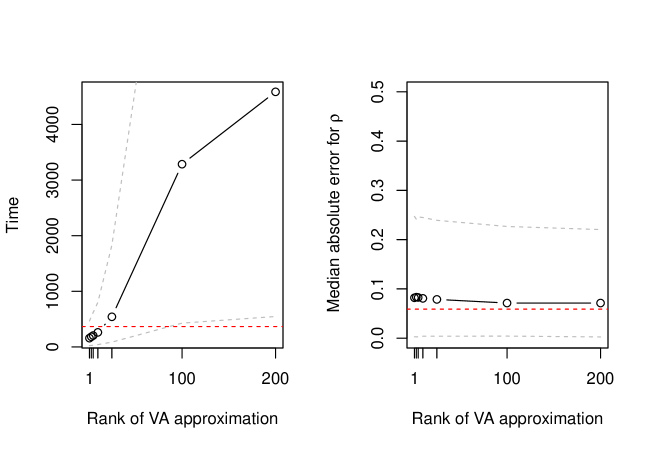
Figure 1: Results of the first simulation study for evaluating the accuracy of the low-rank VA approximation. The left panel displays increase of fitting time with the rank (1, 3, 5, 10, 25, 100, 200) of the VA approximation, where the dashed red line indicates the computation time for the models fitted by Laplace approximation, and the dashed grey lines the 2.5% and 97.5% percentiles. The right panel shows the median absolute error for the phylogenetic signal parameter, which at most can be 0.5. Again, the red line indicates performance of the Laplace approximation and the grey dashed lines the 2.5% and 97.5% percentiles.

The first simulation study confirms that the computation time of the models rapidly increase with the selected rank of the VA approximation, even far beyond the fitting time for the Laplace approximation (indicated by the red dashed line). As seen in the left panel of Figure 1, the rank of the VA approximation had a large impact of the computation time, but fortunately little impact on the estimation accuracy of the phylogenetic signal parameter, which remained nearly stable across various ranks of the VA approximation and was indeed lowest for the full rank approximation.

In the second simulation study we kept the rank of the VA approximation fixed to one, as well as the number of sites fixed to $n=100$, but instead varied the number of species ($m\in\{50,100,250,500\}$) and the number of nearest neighbors used ($nn\in\{3,5,7,9,11,13,15\}$) to approximate the inverse of the phylogenetic covariance matrix. For each combination we simulated 250 datasets, for either binary data or counts. The results are presented in Figure 2.

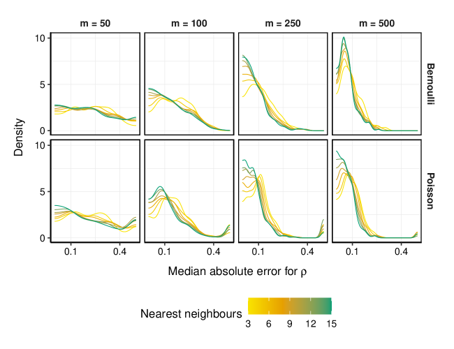
Figure 2: Results for the second simulation study to test the ability of the models to accurately estimate the phylogenetic signal parameter using the low-rank VA and NNGP approximations for different numbers of species $m$ in the data.

The results in Figure 2 represent the compounded approximation error due to both the low-rank VA approximation and the NNGP. The number of species has a larger impact on the estimation accuracy of the phylogenetic signal than the NNGP approximation. As the number of species increase, the estimation accuracy of the phylogenetic signal improved, with $m=50$ being too few species for accurate estimation, but with $m>100$ usually providing accurate estimates. The accuracy was higher with more nearest neighbours, but a relatively low (e.g., 10) number of nearest neighbors seems sufficient for accurate estimates of the phylogenetic signal, even for large numbers of species in the data.

Case study

We demonstrate the new method for fitting phylogenetic random effect models on data collected by Abrego et al. (2022a). The dataset contains the binary responses of 320 wood-inhabiting fungi surveyed on 1809 logs across 53 European beech (Fagus sylvatica) forest sites in different European countries that were grouped into eight regions, so that there were in total $n=1666$ rows in the data. Species with four or less presences were removed before analysis in the original article. Abrego et al. (2022a) fitted JSDMs with the Hmsc R-package with as main goal to determine if traits and phylogenetic relationships structure species communities differently at different spatial scales. To that end, their analyses included environmental variables both at the log- and site-scales such as: diameter at breast height of logs (DBH), decay stage of the logs (on a scale of one to five), an index for connectivity (at the 10km scale), area of forest patches (in hectares), annual temperature range (degrees Celsius) and annual precipitation, and naturally a phylogeny.

Here fit the same four models: three fourth corner models with 1) fruit-body type, (log) spore volume, and trophic group (“lifestyle”; wood decaying or other), 2) Principal Component axes extracted from the matrix of all traits, 3) the first axis due to each a) the reproductive traits, b) dispersal traits, and c) resource use traits, and 4) a model without traits. All models included covariate-specific phylogenetic signal parameters, except for one additional model without traits that was fitted for better comparison with the results from Abrego et al. (2022a). We decided against incorporating latent variables for brevity, and because the gllvm R-package at the time of writing only facilitates including latent variables at the observation level.

In the Hmsc R-package each model takes about a week to 10 days to run (N. Abrego, pers. comm., 1st March 2024), while it takes three to four minutes per model with the methods in this article (on a Dell Latitude 7490 using 7 CPU). This was with 10 nearest neighbors, nested random intercepts for the study region and reserves, and including correlation between covariate effects.

The phylogenetic signal parameter estimates from all models are organised in table 1. Our results deviated somewhat from the original analysis, in that the phylogenetic signal was estimated to be somewhat lower, with 0.51 being the estimated phylogenetic signal for a model without traits, and while assuming the phylogenetic signal to be the same for all covariates, compared to the 0.73 found in the original analysis by Abrego et al. (2022a).

Table 1: Phylogenetic signal parameter estimates for models fitted to the Abrego et al. (2022) data. A parameter estimate near zero is displayed as a blank cell for improved readability.

	No traits(a)	No traits(b)	Group-specific PCA	Raw traits	Overall PCA
Intercept	0.51	0.04	0.04	0.02	0.05
Deadwood size	0.51	0.12	0.01	0.01	0.01
Decay stage	0.51	0.99	0.94	0.85	0.91
Decay stage²	0.51	0.82	0.32	0.18	0.10
Connectivity	0.51	0.73	0.59	0.49	0.47
Temperature range	0.51	0.06	0.02
Precipitation	0.51	0.69	0.64	0.57	0.68
ln(Reserve area)	0.51	0.43	0.39	0.42	0.53

The Hmsc R-package is presently unable to estimate covariate-specific phylogenetic signal parameters, so that Abrego et al. (2022a) post-hoc retrieved estimates of phylogenetic signal by fitting phylogenetic regressions to the posterior distributions of the covariate effects, using the ape R-package. At the deadwood-unit level, they found species responses to decay stage, and decay stage² to be phylogenetically structured, and at the forest-site level they found reserve area, and in some models connectivity, to be phylogenetically structured. Abrego et al. (2022a) did not find a statistically significant result for the effect of precipitation.

At the deadwood-unit level, we similarly find species responses to decay stage to be phylogenetically structured in all of the fitted models, and when traits are absent also to decay stage². At the forest-site level, we are able to corroborate the result by Abrego et al. (2022a) that species responses to connectivity and reserve area are phylogenetically structured to some degree, though we additionally find species responses to precipitation to be phylogenetically structured. Consequently, although the exact numerical values differ, we find similar phylogenetic structuring at both spatial scales present in the study, but while fitting the model in a single step and much more quickly.

For further visual presentation of the results we have chosen the model with the original trait variables. This was ranked lowest by AIC, and provides the most straightforward interpretation (unlike the models that include Principal Component axes). This result confirms that species responses were indeed structured by functional traits. Figure 3 displays the phylogeney with the predicted phylogenetic random effects, as well as the community mean responses, and Figure 4 displays the joint effects of the community mean response and the effect of trait on species responses, with their 95% confidence interval bands (see appendix S3 for a visualization of the marginal trait-environment effects).

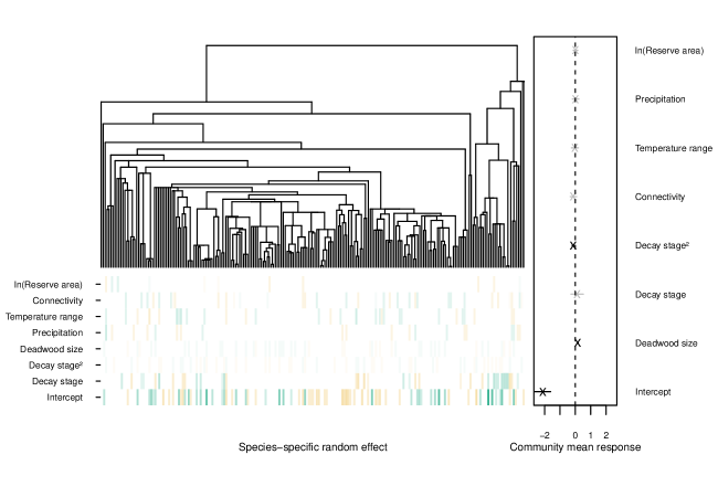
Figure 3: The left panel displays community mean responses to the covariates, with 95% confidence intervals. Coefficients are greyed out of the confidence interval crosses zero, so that it is unclear if there is an effect of a covariate on the community. The bottom panel presents species-specific deviations from the community mean effects. A species-specific effect of zero is interpreted as lack of evidence that a species responds differently to the environment than the community mean response. Orange colors indicate a more negative response than the community mean effect, and green more positive. Species effects of which the prediction interval included zero have been removed.

For the intercept, dead wood size, and decay stage² there was sufficient evidence to conclude a non-zero community mean response. The estimate for decay stage² was negative, and predicted species-specific random effects generally smaller than the community mean response, corresponding to typically expected unimodal (bell-shaped) curves that open downward (i.e., with maxima).

Species responses to deadwood size were positive on average, but become increasly less positive with an increase in spore volume, with Corticioid fruit-body types having the least positive response and Polyporoid pileate fruit-body types the most positive. The effect of decay stage is difficult to disentangle due to the additional quadratic term in the model, though the effect of the quadratic term can be used to infer how species tolerances change with traits (van der Veen et al. 2021). Polyporoid resupinate and Polyporoid pileate fruit-body types exhibit a more narrow tolerance to changes in decay stage than Stromatoid fruit-body types, i.e., they are more sensitive to change in decay stage of deadwood.

Wood decaying fungi were most positively affected by connectivity of the forest among fungi species, and by the size of the reserve. Fungi generally exhibited increased presence to improved connectivity of the forest, and wood-decaying fungi with large spore volume especially so. Fungi with larger spore volume exhibited a more negative response to precipitation than species with a small spore volume. Finally, wood-decaying fungi are among the most prevalent fungi types in larger reserves.

Figure 4: Predicted species responses to the environment from the model as a function of traits, with 95% confidence interval bands. Grey points represent the estimated species responses to the environmental covariates. Different fruit-body types are represented as different color lines, whether fungi are wood-decaying as dashed lines, and the final trait of spore volume is visualized on the horizontal axes

Discussion

In this article, we developed a new method for quickly fitting phylogenetic random effects models, akin to the approaches in the phyr (A. Ives et al. 2020), Hmsc (Tikhonov et al. 2024), and MCMCglmm (Hadfield 2010) R-packages. Because our models are developed as part of the gllvm R-package (Niku et al. 2023), the software supports a wide range of response types, including for Bernoulli, (zero-inflated) Poisson and negative-binomial, Tweedie, and beta responses (Korhonen et al. 2021; Niku et al. 2017; Hui et al. 2017).

By utilizing approximate likelihood methods, the models are magnitudes faster to fit than in the Hmsc and MCMCglmm R-packages, which are based on Markov chain Monte Carlo methods. By applying two more approximations, namely a low-rank VA approximation and NNGPs (Finley et al. 2019) computation time of the proposed models is reduced as much as possible. Two sets of simulation studies confirm that the proposed combination of approximations still enjoys accurate estimation of the phylogenetic signal parameter, while significantly speeding up model fitting.

Unlike in models fitted with the Laplace approximation, we here mostly fitted the models using VA. In this article we purposefully limited the flexibility of the approximation to fit phylogenetic random effects models even more quickly. The flexibility of VA is determined by the number of hyperparameters introduces to the likelihood, which are estimated together with the model parameters. Especially for VA, we find that a good optimisation routine, besides decent initial values, is critical for successful and speedy convergence of the models. In our experience, limited-memory optimisation algorithms (Nocedal and Wright 2006) often lead to faster model fitting and convergence, and an improved ability to successfully leverage methods for parallel computation. In future research we hope to explore improved optimisation routines (as in van der Veen 2024), and their ability to more efficiently fit mixed effects models.

Using real data on 215 species of wood-inhabiting fungi (Abrego et al. 2022b), we demonstrated application of the methods. One of the main novelties of the proposed approach for fitting phylogenetic random effects models is the ability to estimate phylogenetic signal separately for each covariate, without the need to introduce an additional set of random effects as in the phyr R-package, and while simultaneously facilitating the estimation of correlation between random effects for different environmental covariates. Abrego et al. (2022a) fitted various models with and without traits to determine if phylogenetic structuring of species responses occurred at multiple spatial scales simultaneously: at the forest site-scale and at the scale of deadwood logs. Abrego et al. (2022a) post-hoc estimated covariate-specific phylogenetic signal, while here we estimated the covaritae-specific phylogenetic signal directly as part of the model, and while fitting the models in minutes, rather than days as in the Hmsc R-package. Our results largely confirm their findings, namely that fungi responses to decay stage, precipitation, connectivity, and reserve area are phylogenetically structured. We here also find species responses to precipitation are phylogenetically structured.

The phylogenetic signal parameter represents the degree to which species environmental responses are phylogenetically structured, and the associated variance of covariates the rate at which the responses evolve. When the phylogenetic signal parameter is one, species responses to an environmental covariate are fully phylogenetically structured, and at zero the responses are independent (Pearse, Davies, and Wolkovich 2023). The reason for the presence of phylogenetic signal, or the lack thereof, cannot be discerned from phylogenetic random effects models directly. When there is phylogenetic signal, this can be due to the lack of (phylogenetically structured) traits in the model, because the measured traits are not phylogentically structured, or because they are structured in a way that disagrees with the structuring in species environmental responses. In contrast, a lack of phylogenetic signal may be because traits in the model sufficiently introduce phylogenetic structuring to the species responses, because there is no ongoing evolution in the trait that is species environmental responses, or because evolution moves so rapidly that closely related species are (apparently) so different that their environmental responses are independent.

An interesting avenue for future research is to extend the model to incorporate both phylogenetic attraction and repulsion. In their current form phylogenetic random effect models only incorporate positive species associations, meaning that more closely related species can occur in more similar environments. This makes sense if closely related species segregate their resource utilization. However, two closely related species that share the same resource would be more likely to occur in different environments, i.e., exhibit a negative association. Phylogenetic repulsion can be modelled in the current framework, by prior to model fitting replacing the phylogenetic correlation matrix by its inverse (A. R. Ives and Helmus 2011). Still, the current model is limited to either attraction or repulsion, and ideally its form should be adjusted to allow the data to drive that decision instead.

Data availability

The data used in this study is available online (Abrego et al. 2022b).

References

References

- Abrego, Nerea, Claus Bässler, Morten Christensen, and Jacob Heilmann-Clausen. 2022a. “Traits and Phylogenies Modulate the Environmental Responses of Wood-Inhabiting Fungal Communities Across Spatial Scales.” Journal of Ecology 110 (4): 784–98. https://doi.org/10.1111/1365-2745.13839.
- ———. 2022b. “Data and Code from: Traits and Phylogenies Modulate the Environmental Responses of Wood-Inhabiting Fungal Communities Across Spatial Scales.” Dryad. https://doi.org/10.5061/DRYAD.T76HDR82R.
- Bates, Douglas, Martin Mächler, Ben Bolker, and Steve Walker. 2015. “Fitting Linear Mixed-Effects Models Using lme4.” Journal of Statistical Software 67 (1): 1–48. https://doi.org/10.18637/jss.v067.i01.
- Braga, João, Cajo J. F. ter Braak, Wilfried Thuiller, and Stéphane Dray. 2018. “Integrating Spatial and Phylogenetic Information in the Fourth-Corner Analysis to Test Trait–Environment Relationships.” Ecology 99 (12): 2667–74.
- de Villemereuil, Pierre, and Shinichi Nakagawa. 2014. “General Quantitative Genetic Methods for Comparative Biology.” In Modern Phylogenetic Comparative Methods and Their Application in Evolutionary Biology: Concepts and Practice, edited by László Zsolt Garamszegi, 287–303. Berlin, Heidelberg: Springer. https://doi.org/10.1007/978-3-662-43550-2_11.
- Finley, Andrew O., Abhirup Datta, Bruce D. Cook, Douglas C. Morton, Hans E. Andersen, and Sudipto Banerjee. 2019. “Efficient Algorithms for Bayesian Nearest Neighbor Gaussian Processes.” Journal of Computational and Graphical Statistics 28 (2): 401–14. https://doi.org/10.1080/10618600.2018.1537924.
- Hadfield, Jarrod D. 2010. “MCMC Methods for Multi-Response Generalized Linear Mixed Models: The MCMCglmm R Package.” Journal of Statistical Software 33 (2): 1–22.
- Hui, Francis K. C., Sara Taskinen, Shirley Pledger, Scott D. Foster, and David I. Warton. 2015. “Model-Based Approaches to Unconstrained Ordination.” Methods in Ecology and Evolution 6 (4): 399–411. https://doi.org/10.1111/2041-210X.12236.
- Hui, Francis K. C., David I. Warton, John T. Ormerod, Viivi Haapaniemi, and Sara Taskinen. 2017. “Variational Approximations for Generalized Linear Latent Variable Models.” Journal of Computational and Graphical Statistics 26 (1): 35–43. https://doi.org/10.1080/10618600.2016.1164708.
- Ives, Anthony R, and Matthew R Helmus. 2011. “Generalized Linear Mixed Models for Phylogenetic Analyses of Community Structure.” Ecological Monographs 81 (3): 511–25.
- Ives, Anthony, Russell Dinnage, Lucas A. Nell, Matthew Helmus, and Daijiang Li. 2020. Phyr: Model Based Phylogenetic Analysis. Manual.
- Korhonen, Pekka, Francis K. C. Hui, Jenni Niku, and Sara Taskinen. 2021. “Fast, Universal Estimation of Latent Variable Models Using Extended Variational Approximations.” arXiv:2107.02627 [Stat], July. https://arxiv.org/abs/2107.02627.
- Korhonen, Pekka, Francis K. C. Hui, Jenni Niku, Sara Taskinen, and Bert van der Veen. 2024. “A Comparison of Joint Species Distribution Models for Percent Cover Data.” arXiv Preprint arXiv:2403.11562. https://arxiv.org/abs/2403.11562.
- Kristensen, Kasper, Anders Nielsen, Casper W Berg, Hans Skaug, and Brad Bell. 2015. “TMB: Automatic Differentiation and Laplace Approximation.” arXiv Preprint arXiv:1509.00660. https://arxiv.org/abs/1509.00660.
- Matsuba, Misako, Keita Fukasawa, Satoshi Aoki, Munemitsu Akasaka, and Fumiko Ishihama. 2024. “Scalable Phylogenetic Gaussian Process Models Improve the Detectability of Environmental Signals on Local Extinctions for Many Red List Species.” Methods in Ecology and Evolution 15 (4): 756–68. https://doi.org/10.1111/2041-210X.14291.
- Niku, Jenni, Wesley Brooks, Riki Herliansyah, Francis K. C. Hui, Pekka Korhonen, Sara Taskinen, Bert van der Veen, and David I. Warton. 2023. “Gllvm: Generalized Linear Latent Variable Models. R Package Version 1.4.3.”
- Niku, Jenni, Francis K. C. Hui, Sara Taskinen, and David I. Warton. 2021. “Analyzing Environmental-Trait Interactions in Ecological Communities with Fourth-Corner Latent Variable Models.” Environmetrics 32 (6): e2683. https://doi.org/10.1002/env.2683.
- Niku, Jenni, David I. Warton, Francis K. C. Hui, and Sara Taskinen. 2017. “Generalized Linear Latent Variable Models for Multivariate Count and Biomass Data in Ecology.” Journal of Agricultural, Biological and Environmental Statistics 22 (4): 498–522. https://doi.org/10.1007/s13253-017-0304-7.
- Nocedal, Jorge, and Stephan J. Wright. 2006. Numerical Optimization. Springer Series in Operations Research and Financial Engineering. Springer New York. https://doi.org/10.1007/978-0-387-40065-5.
- Ormerod, John T, and Matt P Wand. 2010. “Explaining Variational Approximations.” The American Statistician 64 (2): 140–53.
- Ovaskainen, Otso, Gleb Tikhonov, Anna Norberg, F. Guillaume Blanchet, Leo Duan, David Dunson, Tomas Roslin, and Nerea Abrego. 2017. “How to Make More Out of Community Data? A Conceptual Framework and Its Implementation as Models and Software.” Ecology Letters 20 (5): 561–76. https://doi.org/10.1111/ele.12757.
- Pagel, Mark. 1999. “Inferring the Historical Patterns of Biological Evolution.” Nature 401 (6756): 877–84. https://doi.org/10.1038/44766.
- Paradis, Emmanuel, and Klaus Schliep. 2019. “Ape 5.0: An Environment for Modern Phylogenetics and Evolutionary Analyses in R.” Bioinformatics (Oxford, England) 35: 526–28. https://doi.org/10.1093/bioinformatics/bty633.
- Pearse, William D., T. Jonathan Davies, and E. M. Wolkovich. 2023. “How to Define, Use, and Interpret Pagel’s (Lambda) in Ecology and Evolution.” bioRxiv. https://doi.org/10.1101/2023.10.10.561651.
- Pinheiro, José C., and Douglas M. Bates. 1996. “Unconstrained Parametrizations for Variance-Covariance Matrices.” Statistics and Computing 6 (3): 289–96. https://doi.org/10.1007/BF00140873.
- Pollock, Laura J., Reid Tingley, William K. Morris, Nick Golding, Robert B. O’Hara, Kirsten M. Parris, Peter A. Vesk, and Michael A. McCarthy. 2014. “Understanding Co-Occurrence by Modelling Species Simultaneously with a Joint Species Distribution Model (JSDM).” Methods in Ecology and Evolution 5 (5): 397–406. https://doi.org/10.1111/2041-210X.12180.
- Tikhonov, Gleb, Otso Ovaskainen, Jari Oksanen, Melinda de Jonge, Oystein Opedal, and Tad Dallas. 2024. Hmsc: Hierarchical Model of Species Communities. Manual.
- van der Veen, Bert. 2024. Minic: Minimization Methods for Ill-Conditioned Problems. Manual.
- van der Veen, Bert, Francis K. C. Hui, Knut A. Hovstad, and Robert B. O’Hara. 2023. “Concurrent Ordination: Simultaneous Unconstrained and Constrained Latent Variable Modelling.” Methods in Ecology and Evolution 14 (2): 683–95. https://doi.org/10.1111/2041-210X.14035.
- van der Veen, Bert, Francis K. C. Hui, Knut A. Hovstad, Erik B. Solbu, and Robert B. O’Hara. 2021. “Model-Based Ordination for Species with Unequal Niche Widths.” Methods in Ecology and Evolution 12 (7): 1288–1300. https://doi.org/10.1111/2041-210X.13595.
- Warton, David I., F. Guillaume Blanchet, Robert B. O’Hara, Otso Ovaskainen, Sara Taskinen, Steven C. Walker, and Francis K. C. Hui. 2015. “So Many Variables: Joint Modeling in Community Ecology.” Trends in Ecology & Evolution 30 (12): 766–79. https://doi.org/10.1016/j.tree.2015.09.007.