A Psychology-based Unified Dynamic Framework for Curriculum Learning

Abstract

Directly learning from examples of random difficulty levels is often challenging for both humans and machine learning models. A more effective strategy involves exposing learners to examples in a progressive order, from easy to difficult. Curriculum Learning (CL) has been proposed to implement this strategy in machine learning model training. However, two key challenges persist in CL framework design: defining the difficulty of training data and determining the appropriate amount of data to input at each training step. This paper presents a Psychology-based Unified Dynamic Framework for Curriculum Learning (PUDF), drawing inspiration from psychometrics. We quantify the difficulty of training data by applying Item Response Theory (IRT) to responses from Artificial Crowds (AC). This theory-driven IRT-AC approach leads to global (i.e., model-independent) and interpretable difficulty values. Leveraging IRT, we propose a Dynamic Data Selection via Model Ability Estimation (DDS-MAE) strategy to schedule the appropriate amount of data during model training. Since our difficulty labeling and model ability estimation are based on a consistent theory, namely IRT, their values are comparable within the same scope, potentially leading to a faster convergence compared to the other CL methods. Experimental results demonstrate that fine-tuning pre-trained language models with PUDF enhances their performance on the GLUE benchmark. Moreover, PUDF surpasses other state-of-the-art (SOTA) CL methods on the GLUE benchmark. We further explore the components of PUDF, namely the difficulty measurer (IRT-AC) and the training scheduler (DDS-MAE) qualitatively and quantitatively. Lastly, we conduct an ablation study to clarify which components of PUDF contribute to faster convergence and higher accuracy.

1 Introduction

Curriculum learning (CL) is an effective machine learning framework that trains models by gradually introducing examples of increasing difficulty (Bengio et al., 2009). CL has demonstrated its power in improving the generalization capacity and convergence rate of various models in a wide range of scenarios such as computer vision (CV, Soviany et al., 2021; Zhang et al., 2021), natural language processing (NLP, Zhan et al., 2021; Zhao et al., 2021), robotics (Milano and Nolfi, 2021; Manela and Biess, 2022), and medical applications (Liu et al., 2022; Burduja and Ionescu, 2021). In NLP in particular, CL has demonstrated significant improvements in various applications, including machine translation (Zhan et al., 2021; Mohiuddin et al., 2022), sentiment analysis (Cirik et al., 2016; Tsvetkov et al., 2016), and natural language understanding (Xu et al., 2020). The success of CL can be attributed to its ability to guide the training process towards optimal regions in the parameter space, thus reducing time spent on noisy and difficult samples in early training stages (Wang et al., 2021).

Recent advancements in NLP have greatly benefited from pre-trained language models (PLMs) such as BERT (Kenton and Toutanova, 2019) and T5 (Raffel et al., 2020). These PLMs play a crucial role in enabling models to perform tasks with domain-specific expertise. With PLMs has come a widely adopted two-step process for model fitting: pre-training and fine-tuning. During the pre-training stage, PLMs acquire general knowledge through self-supervised learning on extensive corpora. Subsequently, they are fine-tuned on specific tasks using carefully labeled, domain-specific datasets. While fine-tuning PLMs for many downstream NLP tasks often yields impressive performance improvements (Guo et al., 2022; Kalyan et al., 2021), this strategy is not without its imperfections. Specifically, the standard fine-tuning paradigm does not consider the difficulty of individual training examples, instead feeding them to the model in random order, ignoring the various complexities of data samples and the learning status of the current model. This randomness can potentially lead to inefficient learning (Bengio et al., 2009; Wang et al., 2021), as the model may waste time on overly difficult or noisy examples too early in the training process, potentially hindering overall performance.

A recent survey on CL provided a general taxonomy of CL methods based on two key components (Wang et al., 2021): a difficulty measurer (DM) to define the difficulty of the training data and a training scheduler (TS) to select data during fine-tuning. Wang et al. (2021) categorize current CL methods into four types based on how the DM and TS are implemented. Pre-defined CL relies on heuristics (e.g., the length of sentence or the rarity of the words) for DM and a predetermined scheduling function (e.g., a linear function or root function) for TS (Platanios et al., 2019; Spitkovsky et al., 2010). While simple and often effective, it is challenging to find the optimal combination of DM and TS for specific tasks and datasets, often requiring expert domain knowledge. Moreover, examples that are easy for humans may not be easy for models due to different decision boundaries (Yuan et al., 2019). Self-paced learning-based CL (SPL) utilizes the current model’s training loss as DM (Kumar et al., 2010; Jiang et al., 2015). SPL is more automatic and more aligned with the model’s learning process; however, early training may incur high uncertainty when the model is not yet sufficiently trained. Moreover, it still uses a predetermined function as TS. Transfer teacher-based CL employs another stronger PLM as a teacher model DM to assess data difficulty by fine-tuning it on the training dataset in advance (Xu et al., 2020; Maharana and Bansal, 2022). This method is costly due to the additional fine-tuning and still relies on a predefined TS. Reinforcement learning (RL) teacher-based CL method automatically conducts DM and TS (Zhao et al., 2020; Kumar et al., 2019). The DM is taken as the action in the RL schemes, and the student model feedback is taken as the state and reward. However, this method is even more expensive than the transfer teacher-based CL, requiring fine-tuning of both the teacher and RL models for each epoch, along with a carefully designed reward function to facilitate TS.

To address these challenges, we propose a novel CL framework, Psychology-based Unified Dynamic Framework for Curriculum Learning (PUDF). PUDF automatically estimates both the difficulty of examples and the ability of models as latent variables in a theoretically grounded way. PUDF introduces two novel approaches to the DM and TS components of the CL framework: Item Response Theory-based Artificial Crowds (IRT-AC) as the DM and Dynamic Data Selection via Model Ability Estimation (DDS-MAE) as the TS. IRT-AC is based on Item Response Theory (IRT), a well-established methodology in psychometrics used for test construction and subject evaluation (Baker and Kim, 2004; De Ayala, 2013). IRT models can be applied to estimate latent parameters for example difficulty and subject ability. Traditionally, fitting IRT models requires extensive human-annotated data. However, recent work has shown that IRT models can be fit using machine-generated data instead of human-generated data (Lalor et al., 2019). Building on this, we propose the use of artificial crowds (AC) composed of multiple high-performing PLMs (e.g., T5 (Raffel et al., 2020), ELECTRA (Clark et al., 2020), DeBERTa (He et al., 2020)) to obtain predicted results of the training data used to estimate an IRT model. Our proposed AC, based on multiple PLMs, enhances diversity and allows for offline completion by fine-tuning the AC on validation datasets, thus amortizing the computational cost. Furthermore, traditional IRT models do not scale well to large numbers of subjects and items. Therefore, we leverage a variational inference (VI) method (Hoffman et al., 2013; Jordan et al., 1999) to fit a large-scale IRT model. The DDS-MAE TS component uses the learned IRT model to estimate latent ability parameters for the model during each training epoch. DDS-MAE dynamically selects training data based on the model’s current ability, similar to RL teacher-based CL, but is able to do so more efficiently by eliminating the need for a carefully designed reward function.

To the best of our knowledge, this is the first work to learn model competency during training that is directly comparable to the difficulty of the examples. Our contributions are as follows (1) We propose PUDF, an innovative approach to implementing an effective CL strategy for fine-tuning PLMs; (2) Compared to existing CL methods, our DM, IRT-AC, and TS, DDS-MAE, automatically define data difficulty and achieve dynamic data selection without significant time penalties; (3) Experimental results demonstrate PUDF’s fast convergence and higher accuracy for fine-tuning PLMs, particularly with large-scale datasets, highlighting its scalability and efficiency.

Prior work

This paper extends work that was first published in Findings of EMNLP (Lalor and Yu, 2020). In this manuscript, we have made significant changes. Specifically, we conduct new experiments with PLMs and benchmark against state of the art curriculum learning methods. We also conduct extensive ablation studies and analyses to better understand how PUDF’s components affect performance.

2 Related Work

In this section, we present an overview of Curriculum Learning (CL). We begin by introducing the fundamental concept of CL, followed by a description of a general framework for CL design (Wang et al., 2021). We then explore the current categories of CL methods, highlighting their distinctive features. Finally, we delve into the theoretical foundations underpinning CL to show how these principles contribute to enhanced model training and performance.

2.1 Curriculum Learning and a General Framework

The concept of training neural networks or transformer networks in a progressively easy-to-difficult manner can be traced back to the work of Elman (1993). Building on these foundations, Curriculum Learning (CL) was formally proposed by Bengio et al. (2009), who evaluated designed CL methods on toy datasets with heuristic measures of difficulty. CL was subsequently revisited from a cognitive perspective (Cer et al., 2017), introducing the shaping procedure where a teacher decomposes a complete task into sub-components.

At its core, CL methods implement model training strategies by progressively moving from easier to harder training data. A recent survey of CL (Wang et al., 2021) abstracted CL to include two key components: a difficulty measurer (DM), which provides some score indicating the relative easiness of each data example; and a training scheduler (TS), which decides the sequence of data subsets throughout the training process based on the judgment from the DM. The general workflow for CL involves first ordering all training examples from easiest to most difficult according to the DM. Subsequently, at each training epoch, the TS samples the appropriate subset of training data and presents it to the model for learning.

2.2 Categorizing CL Methods

CL Category	Difficulty Measurer	Training Scheduler	Complexity	References
Pre-defined	Predefined	Predefined	Low	Bengio et al. (2009); Platanios et al. (2019)
Self-paced learning	Automatic	Predefined	Low	Kumar et al. (2010); Ouyang et al. (2023)
Transfer teacher	Automatic	Predefined	High	Xu et al. (2020) Maharana and Bansal (2022)
RL teacher	Automatic	Automatic	High	Zhao et al. (2020) Kumar et al. (2019)
PUDF (This work)	Automatic	Automatic	Low	This work

Table 1: Summary of curriculum learning methods in the literature.

CL methods can be categorized into two types (Wang et al., 2021): in Predefined CL, both DM and TS are designed using human prior knowledge without data-driven methods. In Automatic CL, one or both of the two components are learned by data-driven models or algorithms. Automatic CL includes self-paced learning-based CL, transfer teacher-based CL, and reinforcement learning (RL) based CL. We provide a summary of the current CL works in Table 1 and discuss the characters of each approach below:

Predefined CL.

Researchers have manually designed various DM techniques based on task-specific data characteristics (Spitkovsky et al., 2010; Platanios et al., 2019; Wei et al., 2016; Tsvetkov et al., 2016). Examples of difficult text for the DM include longer sentences, rare words (Platanios et al., 2019), the number of coordinating conjunctions (e.g., “and”, “or”, Kocmi and Bojar, 2017), and the number of phrases (e.g., prepositional phrases, Tsvetkov et al., 2016). Common training schedulers include linear and root functions (Platanios et al., 2019), which increase the number of training samples at a linear or square pace.

SPL-based CL.

SPL-based CL (Kumar et al., 2010; Wan et al., 2020; Mohiuddin et al., 2022; Ouyang et al., 2023) allows the model itself to be the DM according to its loss or other metrics. For example, prior work has used model training loss (Kumar et al., 2010) and pseudo-label predictions (Ouyang et al., 2023) as inputs to the DM to measure learning difficulty. However, model competency is not typically considered in SPL-based CL; instead, it is assumed that competency improves monotonically as more difficult examples are added.

Transfer teacher-based CL.

Transfer teacher-based CL (Weinshall et al., 2018; Xu et al., 2020; Maharana and Bansal, 2022; Hacohen and Weinshall, 2019) employs a pre-trained, “stronger” model as a teacher to to be the DM according to its accuracy. For instance, prior work has used RoBERTa-large (Liu et al., 2019) as the teacher model and a question answering probability function to score the difficulty level of the training data (Maharana and Bansal, 2022). Similarly, a cross-review strategy was proposed where a teacher model with the same structure as the student model labels difficulty (Xu et al., 2020). TS in this transfer teacher-based CL approach leverage predefined functions, such as an annealing method (Xu et al., 2020) or an adaptive function (Maharana and Bansal, 2022).

RL teacher-based CL.

RL teacher-based CL adopts RL models as the teacher to perform TS according to the feedback from the model. Examples of RL teacher methods applied include a multi-armed bandit RL method (Graves et al., 2017), a Q-Learning strategy (Zhao et al., 2020), and a deterministic Actor-Critic RL model (Kumar et al., 2019). This dynamic best approximates the learning process in human education, where the teacher and student improve together through benign interactions: the student makes the biggest progress based on the tailored learning materials selected by the teacher, while the teacher also effectively adjusts her teaching strategy to teach better based on student performance. However, the RL model method is costly; we not only need to train the original model but also fine-tune the RL model during the training. Sometimes the RL model’s training needs more time than the original model’s training.

2.3 Theoretical Analysis of CL

There has been recent work investigating the theory behind CL (Weinshall et al., 2018; Hacohen and Weinshall, 2019), particularly around trying to define an ideal curriculum. CL theoretically leads to a steeper optimization landscape (i.e., faster learning), while keeping the same global minimum of the task without CL. However, these results rely on a “training scheduler,” as opposed to an actual assessment of model ability at a point in time. Theoretical results have also demonstrated a key distinction between CL and similar methods such as self-paced learning (Kumar et al., 2010), hard example mining (Shrivastava et al., 2016), and boosting (Freund and Schapire, 1997): namely that the former considers difficulty with respect to the final hypothesis space (i.e., a model trained on the full data set), while the later methods consider ranking examples according to how difficult the current model determines them to be (Weinshall et al., 2018; Hacohen and Weinshall, 2019). Our proposed PUDF bridges a gap between these methods by probing model ability at the current point in training and using this ability to identify appropriate training examples in terms of global difficulty.

3 Background

In this section, we first introduce IRT, in particular the one-parameter logistic (1PL) model, also referred to as the Rasch model (Rasch, 1960; Baker and Kim, 2004). We describe learning IRT models for machine-learning scale data sets with variational inference methods. Lastly, we introduce our previous work that evaluates data difficulty based on the IRT with DNN-based artificial crowds.

3.1 Item Response Theory

As discussed in the introduction, evaluating the difficulty of the data while considering the model’s capabilities allows for an interpretable comparison between data difficulty and model ability. This runs parallel with an intuitive understanding of human learning, namely that a good student answering a question correctly does not necessarily imply that the question is easy. To achieve this mutual evaluation, we employ item response theory (IRT). IRT methods learn latent parameters of test set examples (called “items” in the IRT literature) and latent ability parameters of individual “subjects.” We refer to “items” as “examples” and “subjects” as “models,” respectively, for clarity and consistency with the curriculum learning literature.

For a model $j$ and an example $i$, the probability that $j$ labels $i$ correctly ($z_{ij}=1$) is a function of the latent parameters of $j$ and $i$. The one-parameter logistic (1PL) model, or Rasch model, assumes that the probability of labeling an example correctly is a function of a single latent difficulty parameter of the example, $b_{i}$, and a latent ability parameter of the model, $\theta_{j}$ (Rasch, 1960; Baker and Kim, 2004):

$$p(z_{ij}=1|\theta_{j},b_{i})=\frac{1}{1+e^{-(\theta_{j}-b_{i})}}$$ (1)

The probability that model $j$ will label item $i$ incorrectly ($z_{ij}=0$) is:

$$p(z_{ij}=0|\theta_{j},b_{i})=1-p(z_{ij}=1|\theta_{j},b_{i})$$ (2)

When plotted, $p(z_{ij}=1|\theta_{j},b_{i})$ is known as an item characteristic curve (ICC). The ICC is a visual representation of the example with regards to how a subject is expected to perform (Fig. 1).

(a)

(b)

Figure 1: Plot of $p(z_{ij}=1|\theta_{j},b_{i})$ as a function of $\theta$ for two examples: (1(a)) an example with difficulty $b=0$, and (1(b)) a more difficult example ($b=2$). Models with ability $\theta_{j}>b_{i}$ (right of dashed line) have greater than 50% chance of labeling the example correctly.

With a 1PL model, there is an intuitive relationship between difficulty and ability. An example’s difficulty value $b$ can be thought of as the point on the ability scale where a model has a 50% chance of labeling an example correctly. Put another way, a model has a 50% chance of labeling an example correctly when model ability is equal to example difficulty ($\theta_{j}=b_{i}$, see Fig. 1).

IRT models that include additional latent parameters such as a guessing parameter for examples exist (e.g., Rodriguez et al., 2021), but in this work we focus on the 1PL model because we are primarily interested in example difficulty and model ability (i.e., $b_{i}$ and $\theta_{j}$).

Fitting an IRT model requires a set of $I$ examples $\{i_{0},i_{1},\dots,i_{I}\}$, a set of $J$ models $\{j_{0},j_{1},\dots,j_{J}\}$, and the binary graded responses of the models to each of the examples, $Z=\{\forall_{i\in I}\forall_{j\in J}:z_{ij}\}$. In our proposed IRT-AC method, the examples are the training dataset, the models correspond to the AC, and the AC’s predicted results correspond to $Z$.

The likelihood of a data set of response patterns $Z$ given the parameters $\Theta$ and $B$ is:

$$\mathcal{L} =\prod_{j=1}^{J}\prod_{i=1}^{I}p(Z_{ij}=z_{ij}|\theta_{j},b_{i})$$ (3)

where $z_{ij}=1$ if individual $j$ answers item $i$ correctly and $z_{ij}=0$ if they do not. The log likelihood is typically considered for computational purposes:

$$\log\mathcal{L} =\sum_{j=1}^{J}\sum_{i=1}^{I}\log p(Z_{ij}=z_{ij}|\theta_{j},b_{i})$$ (4)

For a given data set of response patterns $Z$, item parameters are estimated using a marginal maximum likelihood expectation-maximization algorithm (Bock and Aitkin, 1981), where the latent ability parameters ($\theta$) are assumed to be random effects and integrated out. These methods assume human subjects, and are used for relatively small data sets of no more than a hundred examples or so. The latent ability parameters $\Theta$ are integrated out to define the marginal probability:

E-step: $$\quad p(Z_{ij}=z_{ij}\mid b_{i})=\int_{\theta_{j}}p(Z_{ij}=z_{ij}\mid\theta_{j},b_{i})p(\theta_{j})d\theta_{j}$$ (5)

M-step: $$\quad b_{i}=\arg\max_{b_{i}}\sum\log p(Z_{ij}=z_{ij}\mid b_{i})$$ (6)

VI-IRT approximates the joint posterior distribution $p(\Theta,B|Z)$ by a variational distribution $q(\Theta,B)$:

$$q(\Theta,B) =\prod_{j=1}^{J}\pi^{\theta}_{j}(\theta_{j})\prod_{i=1}^{I}\pi^{b}_{i}(b_{i})$$ (7)

where $\pi^{\theta}_{j}()$ and $\pi^{b}_{i}()$ denote Gaussian densities for different parameters. Parameter means and variances are determined by minimizing the KL-Divergence between $q(\Theta,B)$ and $p(\Theta,B|Z)$:

$$\arg\min_{q}D_{\text{KL}}(q(\Theta,B)||p(\Theta,B|Z))$$ (8)

In selecting priors for VI-IRT, we follow the results of prior work where hierarchical priors were used (Natesan et al., 2016; Lalor et al., 2019). The hierarchical model assumes that ability and difficulty means are sampled from a vague Gaussian prior, and ability and difficulty variances are sampled from an inverse Gamma distribution:

$$\theta_{j}\ |\ m_{\theta},u_{\theta} \sim N(m_{\theta},u^{-1}_{\theta})$$ (9)

$$b_{i}\ |\ m_{b},u_{b} \sim N(m_{b},u^{-1}_{b})$$ (10)

$$m_{\theta},m_{b} \sim N(0,10^{6})$$ (11)

$$u_{\theta},u_{b} \sim\Gamma(1,1)$$ (12)

3.2 IRT with DNN-based Artificial Crowds

A major bottleneck of using IRT methods on machine learning data sets is the fact that each human subject would have to label all (or most) of the examples in order to have enough response patterns to estimate the latent parameters. Gathering enough labels for each example to fit an IRT model would be prohibitively expensive for human annotators. In addition, the annotation quality may be suspect due to the humans labeling upwards of tens of thousands of examples. Therefore, we use artificial crowds (AC) to generate our response patterns. Prior work has shown that this is an effective way to generate a set of response patterns for fitting IRT models to machine learning data (Lalor et al., 2019).

In our original work (Lalor and Yu, 2020), we used deep neural network (DNN) models and trained these models with different subsets of the training data for the artificial crowd (Figure 7 in Appendix A.1). Training data is sub-sampled and corrupted via label flipping so that performance across models in the ensemble is varied. Each trained model then labels all of the training examples, which are graded against the gold-standard label. The output response patterns are used to fit an IRT model for the data.

4 Methodology

Notation	Description
$J$	Artificial crowds
$M$	Model
$Val(X,Y)$	Validation set
$Train(X,Y)$	Training set
$b$	Difficulty parameter of the training data
$\theta$	Ability parameter of the model
$e$	Training epoch
$Z$	Response patterns of the models
$\mathcal{L}$	Likelihood
$q(\Theta,B)$	Variational distribution
$\pi^{\theta}_{j}$	Gaussian density for ability parameters
$\pi^{b}_{i}$	Gaussian density for difficulty parameters
$D_{\text{KL}}$	KL-Divergence
$m_{\theta},m_{b}$	Means of ability and difficulty parameters
$u_{\theta},u_{b}$	Variances of ability and difficulty parameters

Table 2: The descriptions of the notations in our model.

In this section, we first present the workflow for our proposed framework, PUDF, in Section 4.1. We then discuss key insights and challenges for the DM and TS components of PUDF in Sections 4.2 and 4.3, respectively. Additionally, we provide the pseudo-algorithm for PUDF and perform theoretical time complexity analysis in Section 4.4. For clarity, notations and their descriptions are listed in Table 2.

4.1 PUDF workflow

Figure 2: Workflow of the PUDF. The process consists of two main steps: 1) IRT-AC for the DM, 2) DDS-MAE and PLM Fine-tuning for the TS.

The PUDF workflow, as illustrated in Figure 2, comprises two primary steps: 1) IRT-AC based as the DM and 2) DDS-MAE for Fine-tuning as the TS.

To estimate difficulty, the training dataset (for this example, [Q1, Q2, Q3, Q4]) is the input for the artificial crowd (AC). The AC consists of multiple models (here, [M1, M2, M3, M4] representing BERT, T5, GPT-2, and ERNIE) that generate predictions for each training data example. These predictions are evaluated against the true labels and converted to binary outcomes (0 or 1) for each model-data pair. The AC predictions are then used to estimate item difficulty via Item Response Theory, which generates difficulty scores for each training data example (Q1: 1.3, Q2: 1.7, Q3: 0.1, Q4: 2.1), with higher scores indicating greater difficulty.

To schedule training, we evaluate the current PLM’s ability; the PLM generates predictions for the training dataset, which is converted to correct/incorrect responses. Based on the training data examples’ learned difficulty, the PLM’s responses are used to estimate the PLM’s ability (shown as $\theta=1.5$ in the diagram). Based on the difficulty scores from the first step and the PLM’s estimated ability, a subset of the data ([Q1, Q3]), where difficulty (i.e., $b$) is less than ability (i.e., $\theta$), is selected: $b<\theta$. Recall, this leaves only training data for which the model has higher than 50% probability of labeling the example correctly. Subsequently, the selected data subset is used to fine-tune the PLM. The entire second step is iterative: after each epoch, the PLM’s convergence is checked. If fine-tuning has not converged, the process loops back to re-estimate the PLM’s ability and select new data for further fine-tuning. Throughout this process, there is a backward pass (represented by the dashed line) from the fine-tuning step back to updated the PLM weights and refine subsequent predictions, indicating continuous loss optimization.

This workflow combines the strengths of IRT-AC for difficulty estimation, IRT for ability assessment, and dynamic data selection for efficient fine-tuning, resulting in a comprehensive approach to improving PLM performance via CL.

4.2 IRT-AC

IRT-AC provides an effective method for learning item difficulty while accounting for model ability. It consists of two parts: leveraging AC to generate responses and leveraging IRT to generate the difficulty of data. To generate responses via AC, our original work (Lalor and Yu, 2020) employed a DNN-based approach, as detailed in Sec. 3.2. In this study, we leverage multiple PLMs as artificial crowd sources to improve performance. This shift is motivated by several factors:

1. Our previous approach relied on varying noise levels to increase difficulty and therefore the diversity of responses. However, this method yielded monotonous variations, as it considered only a single variant with different levels.

2. In our previous work, the DNN architecture, consisting of only five neural network layers, was relatively simple. In contrast, our currently proposed AC incorporates a range of advanced pre-trained LMs, encompassing encoder-based, decoder-based, and encoder-decoder-based transformer architectures (Vaswani et al., 2017; Kenton and Toutanova, 2019; Brown et al., 2020).

3. Recent research demonstrates that different types of PLMs can help increase the diversity of predicted results on training datasets while maintaining high confidence in their outputs (Bai et al., 2022). Our experimental results (presented in Section 5.5) corroborate these findings.

This refined approach allows us to leverage the predictive performance of PLMs, potentially leading to more robust and diverse difficulty assessments for the IRT-AC method. To further enhance difficulty diversity and increase the credibility of the evaluated difficulty, we perform fine-tuning on the AC PLMs using the validation dataset $Val(X,Y)$ for 1, 3, or 5 epochs. Subsequently, we utilize these fine-tuned AC PLMs to predict labels for the training dataset $Train(X,Y)$, thereby obtaining the response patterns for IRT model fitting. The response patterns generated by the AC in the previous step can be utilized to estimate latent parameters via IRT. Specifically, we fit the IRT model using variational inference (VI) (Natesan et al., 2016; Lalor et al., 2019; Wu et al., 2020) in order to account for the large scale of machine learning datasets (§3.1).

4.3 Dynamic Data Selection via Model Ability Estimation

Another important component in PUDF is Dynamic Data Selection via Model Ability Estimation (DDS-MAE). DDS-MAE aims to train the PLM with examples having smaller difficulty than the model’s ability. The estimated ability of the model at a given epoch $e$, $\hat{\theta}_{e}$, is on the same scale as the difficulty parameters of the data. This establishes a principled approach for selecting data at any given training epoch, namely those examples where $b_{i}\leq\hat{\theta}_{e}$.

Once difficulty values are estimated for the training data, then ability parameters are estimated via maximum likelihood estimation (MLE). Estimating the ability of a model at a point in time is done with an estimation function. In this study, we leverage the Nelder-Mead solver (Lagarias et al., 1998) as the estimation function, also known as the downhill simplex method or the amoeba method, which is a commonly used numerical method for finding the minimum of an objective function in a multidimensional space. When example difficulties are known, model ability is estimated by maximizing the likelihood of the data given the response patterns and the example difficulties (Equation 14). All that is required is a single forward pass of the model on the training data to generate a response pattern (Equation 13).

$$Z_{j} =\forall_{y\in Y}\mathbf{I}[y_{i}=\hat{y_{i}}]$$ (13)

$$\hat{\theta}_{e} =\operatorname*{arg\,max}_{\theta_{e}}\prod_{i=1}^{I}p(z_{ij}=y_{ij}|b_{i})$$ (14)

In our empirical investigations, we encountered two significant challenges. First, the initial evaluated ability of the model is often low, and in some cases, the available training data is limited. This scenario results in insufficient data utilization for model training in the initial epoch, potentially causing the model’s ability to stagnate and impeding further data selection. To mitigate this issue, we implemented an adaptive solution: if the model’s ability fails to improve over two consecutive epochs, we incrementally increase the ability parameter by 0.1. This adjustment enables the training process to overcome initial saddle points and facilitates continued model improvement.

Second, when utilizing the entire training dataset to evaluate the model’s ability, we observed that the IRT calculation time becomes prohibitively long, particularly for large-scale datasets. For instance, the MNLI task from the GLUE benchmark (Wang et al., 2019) comprises approximately 390K data points, and the ability evaluation process for each epoch consumes hundreds of minutes, comparable to the entire model training duration. To address this computational bottleneck, we propose a sampling-based method to evaluate the model’s ability on a randomly selected subset of one thousand data points. This approach effectively balances estimation efficiency and accuracy, significantly reducing computational overhead while maintaining robust ability estimates. These refinements serve to enhance the scalability and efficiency of our framework, enabling its application across a diverse range of tasks and dataset sizes.

4.4 Training process and theoretical analysis

PUDF is a novel CL framework that dynamically selects training examples at each epoch based on the estimated ability of the model at that particular point in time. PUDF leverages a well-established psychometric framework (i.e., IRT) to estimate model ability, ensuring a robust and theoretically grounded approach. The estimated ability of the model at a given epoch $e$, denoted as $\hat{\theta}_{e}$, is calibrated on the same scale as the difficulty parameters of the data. This alignment establishes a principled criterion for data selection at any given training epoch, specifically those examples where $b_{i}\leq\hat{\theta}_{e}$.

Algorithm 1 describes the training procedure in detail. Note that, we assume that example difficulties have been learned offline using existing methods (see §4.2). Each example in the training set has an estimated difficulty parameter ($b_{i}$). The first step of DDS-MAE is to estimate the ability of the model using the estimation function (§4.3, Alg. 1 line 9). To do this, we use part of the training set, but crucially, only to get response data, not to update parameters (i.e., no backward pass). We do not use a held out validation set for estimating ability because we do not want the validation set to influence training. In our experiments, the validation set is only used for early stopping. Model outputs are obtained for the training set, and graded as correct or incorrect as compared to the gold standard label (Alg. 1 line 2). This response pattern is then used to estimate model ability at the current epoch ($\hat{\theta}_{e}$, Alg. 1 line 3).

Once ability is estimated, data selection is done by comparing estimated ability to the examples’ difficulty parameters. If the difficulty of an example is less than or equal to the estimated ability, then the example is included in training for this epoch. Examples where the difficulty is greater than estimated ability are not included (Alg. 1 line 10). Finally, the model is trained with the training data subset (Alg. 1 line 11).

With PUDF, the training data size does not have to be monotonically increasing. PUDF adds or removes training data based not on a fixed step schedule but rather by probing the model at each epoch and using the estimated ability to match data to the model. This way if a model has a high estimated ability early in training, then more data can be added to the training set more quickly, and learning is not artificially slowed down due to the curriculum schedule. If a model’s performance suffers when adding data too quickly, then this will be reflected in lower ability estimates, which leads to less data selected in the next epoch.

Algorithm 1 Training process with DDS-MAE

Input: Data ($X$, $Y$), model $M$, difficulties $B$, num_epochs       Output: Learned model $M^{\prime}$

1:procedure ability_est($Y,\hat{Y},B$)

2:     $Z=\forall_{y\in Y}\mathbf{I}[y_{i}=\hat{y_{i}}]$

3:     $\hat{\theta}_{e}=\operatorname*{arg\,max}_{\theta}p(Z|\theta,b)$

4:     return $\hat{\theta_{e}}$

5:end procedure

6:$M^{\prime}=M$

7:for $e$ in num_epochs do

8:     $\hat{Y}=M^{\prime}(X)$

9:     $\hat{\theta}_{e}=ABILITY\_EST(Y,\hat{Y},D)$

10:     $X_{e},Y_{e}=\{(x,y):b_{i}\leq\hat{\theta}_{e}\}$

11:     $M^{\prime}=train(M^{\prime},X_{e},Y_{e})$

12:end for

13:return $M^{\prime}$

Time complexity analysis

In comparison to conventional model training, our DDS-MAE approach introduces two additional steps: model ability estimation and training data filtering (Alg. 1, lines 9 and 10). The model ability estimation procedure consists of (i) comparing each prediction with its corresponding true label, with a time complexity of $O(N)$, where $N$ is the number of estimated training examples; and (ii) Maximum Likelihood Estimation (MLE) using the Nelder-Mead method, as described in section 4.3, with a time complexity of $O(KN)$, where $K$ is the number of optimization iterations (typically, $K=10$). The training data filtering step also exhibits linear complexity, $O(N)$. Consequently, the total time complexity for DDS-MAE is $O(N)+O(KN)+O(N)=O(KN)$. For conventional transformer-based model training in each epoch, the time complexity is $O(KN^{\prime}/BL(n^{2}d+nd^{2}))$ (Khan et al., 2022; Tay et al., 2022), where $K$ is the number of optimization iterations, $N^{\prime}$ is the number of training data, $B$ is the batch size, $L$ is the number of layers, $n$ is the sequence length, and $d$ is the data dimension. Theoretically, our proposed method is asymptotically equivalent to the conventional training process. We have further experimentally verified the additional time required, demonstrating that DDS-MAE adds at most $5.48\%$ to the training time (§4.4).

In the DM (IRT-AC), we have two parts: the AC to generate the responses and the VI-IRT to calculate the difficulty. For the AC, similar to transformer-based model training, the time complexity is $O(KMN^{\prime\prime}/BL(n^{2}d+nd^{2}))$, where $M$ is the number of models in the artificial crowd and $N^{\prime\prime}$ is the size of the validation set. For VI-IRT, the time complexity is $O(KN)$. We note here that the complexity associated with IRT-AC is an offline cost that, once run, generates difficulty values that can be reused. Once the difficulty parameters of the training data are estimated, they can be used for multiple training runs. We therefore consider this cost as a one-time, offline cost.

5 Experiments

In this section, we first introduce the experimental setup in Section 5.1. Subsequently, we validate PUDF’s performance and compatibility across different PLM models and compare PUDF with other advanced CL methods in Sections 5.2 and 5.3, respectively. We then conduct an ablation study in Section 5.4 to demonstrate the contribution of each component to PUDF’s overall performance. Finally, section 5.5 explores the key components of PUDF: IRT-AC and DDS-MAE.

5.1 Experimental Setup

Datasets

Following recent CL studies in NLP (Sengupta et al., 2023; Maharana and Bansal, 2022; Wan et al., 2020; Xu et al., 2020), we evaluate PUDF on 11 natural language understanding tasks from the GLUE (Wang et al., 2019) benchmark. Dataset summary statistics are provided in Table 3. We exclude the WNLI dataset due to dataset construction inconsistencies.

Because test set labels for our tasks are only available via the GLUE evaluation server we use the held-out validation sets to measure performance, consistent with prior work. For training, we use a 90%-10% split of the training data and use the 10% split as our held-out validation set for early stopping. We can then use the full validation set as our test set to evaluate performance across experiments without making multiple submissions to the GLUE server. Brief descriptions of these tasks follow.

MNLI

Multi-Genre Natural Language Inference, a textual entailment (Bowman et al., 2015) data set collected from ten different sources and human annotated by crowdsource workers (Williams et al., 2018).

QQP

Quora Question Pairs, a data set of questions pairs where the goal is to determine if the questions are duplicates.

QNLI

Question Answering NLI, a modified version of the Stanford Question Answering Dataset (SQuAD) where the goal is to determine if the context sentence determines the answer to the source question (Rajpurkar et al., 2016; Wang et al., 2019).

SST-2

Stanford Sentiment Treebank, a sentiment analysis data set that consists of snippets of text from movie reviews and human-annotated sentiment scores (Socher et al., 2013).

MRPC

Microsoft Research Paraphrase Corpus, a data set of automatically extracted online news sentence pairs and binary human annotations indicating whether the pairs are semantically equivalent or not (Dolan and Brockett, 2005).

RTE

Recognizing Textual Entailment, a binary NLI data set consisting of data from annual NLI challenges (Bentivogli et al., 2009).

GLUE
Dataset	Train	Validation	Test
MNLI	353k	39k	9.8k
MRPC	3.3k	366	409
QNLI	94k	10k	5.5k
QQP	327k	36k	40k
RTE	2.2k	249	278
SST-2	61k	6.7k	873

Table 3: Statistics for GLUE benchmark datasets.

Models

We test the effectiveness and compatibility of PUDF by integrating it with different types of transformer architectures, including encoder-based, decoder-based, and encoder-decoder-based models.

DeBERTaV3

(He et al., 2022) (86M parameters) is an encoder-based pre-trained language model by Microsoft. It uses a disentangled attention mechanism to better capture word dependencies and contextual information, enhancing performance on various natural language understanding tasks.

GPT-2

(Radford et al., 2019) (124M parameters) is a large-scale decoder-based language model by OpenAI. Trained on diverse internet text, it excels in generating coherent, contextually relevant text for tasks like translation, summarization, and question-answering without task-specific training data.

T5

(Raffel et al., 2020) (Text-To-Text Transfer Transformer, 220M parameters) is an encoder-decoder model by Google Research. It frames all NLP tasks as text-to-text problems, allowing application to various tasks such as translation, summarization, and question answering using task-specific prefixes and appropriate input-output text pairs.

Benchmark CL Methods

To benchmark the performance of our proposed PUDF framework, we compare several CL methods that cover each of the four CL categories, i.e., predefined CL, self-paced learning, transfer teacher, and RL teacher.

Pre-defined CL

We evaluate the pre-defined CL based on the paper (Platanios et al., 2019). For the DM, we use the sentence length ($d_{SL}$) or word rarity $d_{WR}$. For the TS, we use a linear or root function to adjust the training pace. We set the initial competency ($c_{0}$) $0.01$ and set the point where the model is fully competent ($T$) to be equal to $total\_epochs/2$ (i.e., the pre-defined CL reaches competency halfway through training and trains with the full training set for the second half) as per the original paper.

Self-paced learning (SPL)

We evaluate a novel self-paced learning algorithm (Zhang et al., 2024) that incorporates belief functions to address limitations in traditional SPL approaches. The DM combines evidential uncertainty and learning loss to characterize difficulty. The TS adjusts the balance between evidential uncertainty and learning loss across training stages, allowing for more appropriate sample selection as the model improves.

Transfer teacher

We evaluate the transfer teacher-based CL based on recent work (Maharana and Bansal, 2022) that uses Question Answering Probability (QAP) as a DM scoring function, and an adaptive function for TS.

RL Teacher

For RL teacher, we evaluate the MPDistil method (Sengupta et al., 2023). MPDistil is a meta-policy knowledge distillation framework that uses a reward-based policy learner as DM and a meta-reinforcement learning-based model and reward function as TS.

Hyper-parameter tuning and hardware platform

For the GLUE benchmark dataset, we use a maximum sequence length of 128 and set the batch size to 64. Although we set the the epoch to be 20, we also use early stopping (Yao et al., 2007) on the validation set to save the training time. All the results reported in the paper are obtained from running a grid search on the baseline models; once the optimized hyper-parameters were identified, all of the CL methods follow these parameters. The hyper-parameters include the learning rate from {2e-5, 3e-5}, $\tau$ from { 4.0, 5.0, 6.0, 7.0}, $\alpha$ from 0.4, 0.5, 0.6, and $\beta$ from {80, 90, 100}. The discount factor $\gamma$ is set as $0.99$. All the models are trained with Adam optimizer with weight decay (Loshchilov et al., 2017).

To fit our IRT model, we use the py-irt Python package (Lalor et al., 2019; Lalor and Rodriguez, 2023), which is built on top of the Pyro probabilistic programming language (Bingham et al., 2018). For the artificial crowds, we leverage BERT (Kenton and Toutanova, 2019), DistillBERT (Sanh et al., 2019), RoBERTa (Liu et al., 2019), DeBERTa (He et al., 2020), ALBERT (Lan et al., 2019), XLNet (Yang et al., 2019), ELECTRA (Clark et al., 2020), T5 (Raffel et al., 2020), BART (Lewis et al., 2019), and GPT-2 (Radford et al., 2019). All the PLMs are implemented from the Huggingface. One Tesla V100 GPU is used to conduct all of the experiments. We repeated the experiments three times and reported the mean and standard deviation of the results (Matiisen et al., 2019).

5.2 Incorporating PUDF in PLM Fine-tuning

Table 4: Comparison of the performance of PLMs with and without PUDF on the GLUE benchmark. The table shows accuracy (Acc.) and training time in minutes (TT), with standard deviations (std) calculated from three repeated experiments in parentheses. Bold results indicate those that are statistically significantly better ($p<0.05$) than the baseline.

	Accuracy $\uparrow$							Training Time $\downarrow$
Methods	MNLI	MRPC	QNLI	QQP	RTE	SST-2	Average	MNLI	MRPC	QNLI	QQP	RTE	SST-2	Average
DeBERTaV3	90.22	87.75	93.61	92.15	80.99	95.45	90.03	379.67	7.88	127.12	481.64	5.88	72.51	179.12
	(0.03)	(1.23)	(0.27)	(0.06)	(0.55)	(0.13)	(0.38)	(20.25)	(0.75)	(27.39)	(14.25)	(0.48)	(2.89)	(11.00)
+PUDF	90.69	89.41	94.86	92.88	81.73	96.10	90.95	318.58	4.26	52.10	163.51	2.63	41.19	97.05
	(0.01)	(0.53)	(0.12)	(0.02)	(0.37)	(0.4)	(0.24)	(17.83)	(1.05)	(2.5)	(7.64)	(0.85)	(3.56)	(5.57)
T5	86.36	88.32	92.2	91.31	72.44	93.96	87.43	799.48	9.8	184.33	1109.64	11.38	117.55	372.03
	(0.06)	(1.84)	(0.06)	(0.06)	(2.05)	(0.63)	(0.78)	(250.7)	(1.57)	(17.14)	(362.63)	(1.27)	(11.38)	(107.45)
T5 +PUDF	86.53	91.93	91.64	92.12	73.07	94.42	88.29	411.79	8.06	106.93	545.72	3.54	83.63	193.28
	(0.52)	(0.62)	(1.29)	(0.09)	(0.42)	(0.29)	(0.54)	(28.63)	(0.9)	(6.14)	(171.49)	(0.95)	(6.37)	(35.75)
GPT-2	81.81	79.74	88.19	89.83	65.34	91.7	82.77	479.77	6.7	162.35	637.99	4.00	91.96	230.46
	(0.03)	(0.14)	(0.33)	(0.15)	(0.72)	(0.55)	(0.32)	(32.56)	(0.85)	(21.69)	(146.99)	(0.61)	(12.26)	(35.83)
+PUDF	81.86	79.84	90.55	90.69	67.65	91.82	83.74	272.26	3.49	84.46	310.50	2.57	67.96	123.54
	(0.5)	(0.75)	(2.71)	(3.59)	(4.38)	(0.13)	(2.01)	(3.31)	(0.34)	(2.18)	(102.14)	(0.42)	(2.62)	(18.5)

As Table 4 shows, PUDF consistently enhances both accuracy and training efficiency across multiple PLMs on the GLUE benchmark. On average, PUDF improves accuracy for DeBERTaV3 by $0.92\%$, T5 by $0.86\%$, and GPT-2 by $0.97\%$, while reducing training times by $45.82\%$, $48.05\%$, and $46.39\%$ respectively.

Across individual datasets, PUDF demonstrates varied but generally positive impacts. MRPC shows the most significant accuracy gains, particularly for T5 ($3.61\%$). QNLI and QQP exhibit mixed accuracy results but consistently substantial training time reductions, with DeBERTaV3 achieving a $59.02\%$ reduction on QNLI and a $66.05\%$ reduction on QQP. RTE and SST-2 show modest accuracy improvements across all models, coupled with significant training time reductions, especially for T5 on RTE ($68.89\%$). These results highlight PUDF’s effectiveness in enhancing PLM performance and efficiency across NLP tasks, with particularly strong benefits in reducing computational demands while maintaining or improving accuracy.

We perform statistical comparisons between the original models (DeBERTaV3, T5, and GPT-2) and their PUDF-enhanced versions on the GLUE benchmark. Our null hypotheses are as follows: $H_{0a}$: PUDF does not improve PLMs’ accuracy. $H_{0t}$: PUDF does not reduce PLMs’ fine-tuning time. We reject the null hypothesis at a significance threshold of $\alpha=0.05$. For accuracy improvements, we reject $H_{0a}$ except for T5 on QNLI, GPT-2 on QQP, and three PLMs on RTE. Further investigation into the RTE dataset reveals that similar accuracy results with high standard deviations are the reason we fail to reject $H_{0a}$ on RTE. This high variation is likely due to the relatively smaller data size compared to other datasets.

Regarding training time, we consistently reject $H_{0t}$ across all three PLMs for most datasets. This indicates that PUDF can effectively reduce training time across a wide range of scenarios, except for T5 on MRPC. Overall, based on the statistical significance results, we can summarize that PUDF can improve model accuracy and reduce training time across most scenarios.

5.3 Comparing PUDF with other CL methods

Table 5: Comparison of different CL methods on the DeBERTaV3 model on GLUE benchmark. The table shows accuracy (Acc.) and training time in minutes (TT). $d_{SL}$ and $d_{WR}$ denote sentence length and word rarity, respectively. $L$ and $R$ represent the linear and root functions, respectively. Trans. and RL. denote transfer-teacher and reinforcement learning-based CL methods. Best results are bolded. PUDF significantly outperforms baseline and other CL methods ($p<0.05$), except those marked by ^†.

	Accuracy $\uparrow$							Training Time $\downarrow$
Methods	MNLI	MRPC	QNLI	QQP	RTE	SST-2	Average	MNLI	MRPC	QNLI	QQP	RTE	SST-2	Average
DeBERTaV3	90.22	87.75	93.61	92.15	80.99†	95.45	90.03	379.67	7.88	127.12	481.64	5.88	72.51	179.12
	(0.03)	(1.23)	(0.27)	(0.06)	(0.55)	(0.13)	(0.38)	(20.25)	(0.75)	(27.39)	(14.25)	(0.48)	(2.89)	(11.00)
$d_{SL}$-L	90.00	88.34†	94.11	91.88	77.62	95.76	89.62	473.79	2.10†	111.98	408.78	3.47†	80.02	180.02
	(0.05)	(8.43)	(0.09)	(0.12)	(0.51)	(0.25)	(1.58)	(18.61)	(1.77)	(4.64)	(18.14)	(0.15)	(2.95)	(7.71)
$d_{SL}$-R	89.93	88.94†	93.74	91.92	76.42	95.57	89.42	412.54	1.96†	113.19	378.04	3.47†	65.16	162.39
	(0.08)	(7.86)	(0.26)	(0.12)	(1.70)	(0.35)	(1.73)	(83.97)	(1.21)	(21.66)	(15.62)	(0.31)	(9.37)	(22.02)
$d_{WR}$-L	90.14	88.10†	93.87	91.81	78.07	95.68	89.61	402.49	2.08†	98.08	357.80	2.45†	77.98	156.81
	(0.06)	(8.09)	(0.17)	(0.11)	(11.60)	(0.46)	(3.42)	(12.94)	(1.77)	(4.10)	(14.30)	(1.35)	(6.03)	(6.75)
$d_{WR}$-R	90.05	88.77†	94.12	91.80	77.62	95.95	89.72	370.59	2.38†	98.17	384.37	3.49†	65.51	154.08
	(0.07)	(7.63)	(0.16)	(0.06)	(0.59)	(0.14)	(1.44)	(5.43)	(1.79)	(21.35)	(38.25)	(0.45)	(7.60)	(12.48)
SPL	90.04	89.38†	94.84	92.14	79.18	95.53	90.19	504.20	4.33†	270.23	530.85	7.00	171.25	247.98
	(0.14)	(3.17)	(0.06)	(0.08)	(1.09)	(0.12)	(0.78)	(45.56)	(0.68)	(10.04)	(40.06)	(0.37)	(8.31)	(17.50)
Trans.	89.80	88.38†	93.53†	91.76†	81.29	95.23	90.00	440.05	10.42	186.44	542.95	7.30	108.80	215.99
	(1.41)	(2.11)	(2.17)	(4.34)	(0.89)	(1.02)	(1.99)	(1.02)	(0.06)	(21.25)	(10.08)	(0.72)	(4.09)	(6.20)
RL.	89.72	90.03†	94.38	90.98	80.89	96.07	90.68	587.31	8.43	210.24	489.43	7.47	100.44	233.22
	(0.72)	(1.85)	(0.53)	(1.27)	(0.77)	(0.21)	(0.89)	(23.17)	(0.88)	(21.37)	(46.89)	(1.01)	(11.83)	(17.86)
PUDF	90.69	89.41	94.86	92.88	81.73	96.10	90.95	318.58	4.26	52.10	163.51	2.63	41.19	97.05
	(0.01)	(0.53)	(0.12)	(0.02)	(0.37)	(0.40)	(0.24)	(17.83)	(1.05)	(2.50)	(7.64)	(0.85)	(3.56)	(5.57)

Table 5 presents a comprehensive comparison of various CL methods applied to the DeBERTaV3 model across GLUE benchmark datasets. PUDF demonstrates competitive performance in accuracy while excelling in training efficiency compared to both pre-defined and automatic CL approaches. PUDF achieves an average accuracy of $90.95\%$, which is significantly better than the best-performing comparison method, RL teacher-based CL ($90.68\%$); PUDF also outperforms the best pre-defined CL method (i.e., $d_{WR}$-R with $89.72\%$). In terms of training efficiency, PUDF significantly outperforms all other methods with an average training time of 97.05 minutes. This is substantially lower than learned CL methods like transfer teacher-based CL (215.99 minutes) and RL teacher-based CL (233.22 minutes), and also more efficient than the best pre-defined method $d_{WR}$-L (156.81 minutes). The efficiency gain of PUDF is particularly evident in computationally intensive tasks like QNLI and QQP. While some pre-defined methods like $d_{WR}$-R show a good balance between accuracy and efficiency, they are consistently outperformed by PUDF in both aspects. These results highlight PUDF’s ability to maintain competitive accuracy while dramatically reducing training time compared to other CL approaches.

We further conduct a statistical analysis to evaluate the impact of PUDF compared to other benchmark CL methods ($d_{WR}-R$, SPL, Trans., and RL.). Our null hypotheses for this analysis are: $H_{0a}$: PUDF does not significantly improve model accuracy compared to other methods. $H_{0t}$: PUDF does not significantly reduce model training time compared to other methods. PUDF demonstrates statistically significant improvements in accuracy ($p<0.05$) compared to most methods across several datasets. Notably, PUDF significantly outperforms Trans. on MNLI, QNLI, QQP, RTE, and SST-2, allowing us to reject $H_{0a}$ in these cases. PUDF also shows significant improvements over RL-teacher based CL for MNLI, QNLI, QQP, and SST-2. Comparisons with $d_{WR}-R$ and SPL yield significant results for MNLI, QNLI, and QQP. However, for MRPC, none of the comparisons reach the significance threshold, suggesting that accuracy improvements on this dataset may be less substantial or consistent across methods.

We also see a strong pattern of improvements in training time for PUDF. We observe statistically significant reductions in training time ($p<0.05$) compared to all methods for MNLI, QNLI, QQP, and SST-2, allowing us to confidently reject $H_{0t}$ for these datasets. PUDF also demonstrates significant time reductions compared to most methods for RTE. Interestingly, MRPC is the only dataset where no significant training time improvements were observed, mirroring the accuracy results.

In conclusion, our statistical analysis provides strong evidence that the proposed PUDF method can significantly outperform existing techniques in terms of both accuracy and training efficiency on the GLUE benchmark. The consistent improvements observed, especially for larger datasets like MNLI, QNLI, and QQP, highlight the robustness and effectiveness of PUDF.

5.4 Ablation Study

Table 6: Ablation study on the PUDF with DeBERTaV3 model on the GLUE benchmark. The table shows accuracy (Acc.) and training time in minutes (TT), with standard deviations (std) calculated from three repeated experiments in parentheses. Best results are bolded.

	Accuracy $\uparrow$							Training Time $\downarrow$
Methods	MNLI	MRPC	QNLI	QQP	RTE	SST-2	Average	MNLI	MRPC	QNLI	QQP	RTE	SST-2	Average
$d_{SL}$ + DDS-MAE	88.84	86.93	91.87	90.53	73.49	95.41	87.85	268.42	4.22	62.09	229.44	1.74	77.06	107.16
	(0.37)	(0.51)	(0.75)	(0.19)	(5.01)	(0.20)	(1.17)	(38.40)	(0.65)	(1.70)	(24.21)	(1.25)	(1.99)	(11.37)
$d_{WR}$ + DDS-MAE	88.68	86.52	91.40	90.35	70.04	95.64	87.11	286.68	3.59	62.16	212.84	3.16	77.20	107.61
	(0.27)	(0.46)	(1.05)	(0.23)	(3.46)	(0.12)	(0.93)	(31.59)	(0.87)	(8.17)	(18.56)	(1.67)	(2.41)	(10.55)
IRT-AC + Root	89.98	87.27	94.56	92.12	76.53	96.44	89.48	334.57	3.80	108.52	424.58	3.46	48.78	153.95
	(0.09)	(0.83)	(0.04)	(0.46)	(2.88)	(0.14)	(0.74)	(52.16)	(1.17)	(10.63)	(72.13)	(1.01)	(5.68)	(23.80)
IRT-AC + Linear	89.90	87.80	94.76	92.68	78.62	96.64	90.07	321.68	4.48	76.30	441.47	3.26	77.21	154.07
	(0.16)	(1.06)	(0.12)	(0.11)	(3.07)	(0.53)	(0.84)	(47.68)	(1.66)	(8.79)	(50.84)	(0.91)	(10.17)	(20.01)
IRT-AC + DDS-MAE (PUDF)	90.69	89.41	94.86	92.88	81.73	96.10	90.95	318.58	4.26	52.10	163.51	2.63	41.19	97.05
	(0.01)	(0.53)	(0.12)	(0.02)	(0.37)	(0.40)	(0.24)	(17.83)	(1.05)	(2.50)	(7.64)	(0.85)	(3.56)	(5.57)

In order to clarify the factors contributing to PUDF’s performance in terms of accuracy and training time, we conducted an ablation study. This experiment involves interchanging the DM and TS components between PUDF and pre-defined CL methods. Table  6 presents the results of our ablation study, from which we can draw several conclusions.

In the first part of the experiment, we employed $d_{SL}$ or $d_{WR}$ as the DM in conjunction with DDS-MAE as the TS. The results reveal that DDS-MAE significantly reduces training time compared to rule-based training schedulers (i.e., Linear and Root). Despite the additional time required for dynamic evaluation of model ability in each epoch, this overhead is negligible relative to the overall training time and contributes to improved model convergence. The combination of $d_{SL}$ or $d_{WR}$ with DDS-MAE results in decreased accuracy compared to pre-defined methods (Table 5) and PUDF, while achieving training times comparable to PUDF. Further analysis of the difficulty distributions generated by $d_{SL}$ and $d_{WR}$ reveals a mismatch with the model ability evaluated by DDS-MAE.

In the second part, we utilize IRT-AC as the DM in combination with Linear or Root as the training scheduler. Our findings indicate that accuracy improves compared to pre-defined methods and approaches that of PUDF, suggesting that the difficulty generated by IRT-AC is more suitable for model training than $d_{SL}$ and $d_{WR}$. This underscores the efficacy of the IRT-AC method compared to the rule-based DMs. The training time remains similar to pre-defined methods but is slower than PUDF. This observation is consistent with expectations, as IRT-AC is responsible for labeling data difficulty, while the training scheduler controls the training pace. While combining IRT-AC with Root or Linear schedulers does not significantly improve training convergence, pairing it with DDS-MAE (i.e., PUDF) yields substantial enhancements, demonstrating the importance of complementarity between the DM and TS.

In conclusion, PUDF (IRT-AC + DDS-MAE) consistently outperforms other combinations across GLUE benchmark datasets, demonstrating the synergistic effect of its components. The IRT-AC component enhances model accuracy, while the DDS-MAE algorithm significantly reduces training time, resulting in an efficient and effective CL approach.

5.5 Further Analyses: Exploring the Components of PUDF

In this section, we conduct an in-depth analysis of the proposed PUDF framework, specifically IRT-AC and DDS-MAE. First, we conduct convergence and runtime analyses on DDS-MAE. We then qualitatively analyze hard and easy examples as scored by IRT-AC. Finally, we examine the difficulty distribution and the artificial crowds’ accuracy and confidence in relation to example difficulty as a way to further validate the learned values.

Convergence Analysis

Figure 3: Convergence analysis of PUDF versus Baseline models on GLUE. Circular markers highlight the best validation accuracy achieved by each model.

We evaluate our proposed DDS-MAE component in PUDF and analyze the training convergence. As shown in Figure 3, we can make several observations.

Convergence Speed

Across all tasks, PUDF demonstrates rapid convergence, often reaching competitive accuracy levels within fewer epochs than the baseline. This is particularly evident in MNLI, MRPC, and QNLI, where PUDF’s accuracy curve shows a steep ascent in the early epochs. In contrast, the baseline model typically requires more epochs to reach comparable performance levels. This rapid convergence of PUDF suggests that it can achieve good results with fewer training iterations, potentially saving computational resources.

Data Efficiency

The blue dotted line, representing the percentage of training data used by PUDF, provides crucial insights into its data efficiency. We observe that in the early epochs, not all training data are fed into the model. Initially, only approximately half of the data (with the exception of SST-2) are utilized. As the model’s capability increases during the fine-tuning process, more data are gradually incorporated into the training. This progressive data introduction aligns with the model’s growing ability to handle increasingly complex examples.

Data Usage

In most tasks, PUDF achieves its peak performance using less than $100\%$ of the training data. For instance, in QNLI and QQP, PUDF reaches its best accuracy using around $90\%-95\%$ of the data. This demonstrates PUDF’s ability to prioritize the most informative training examples. Furthermore, this analysis reveals that not all data are equally beneficial for model training. As discussed in our qualitative analysis below, some examples are labeled as the most difficult by IRT-AC due to incompleteness or incorrect labeling. The DDS-MAE can leverage this difficulty information effectively, and schedules these difficult and potentially harmful data points to be trained at a later stage, rather than early on. This strategic ordering helps mitigate their disruptive impact on the model’s learning process.

Accuracy Comparison

In terms of peak validation accuracy (indicated by circular markers), PUDF consistently matches or outperforms the baseline across most tasks. Notably, in MNLI, QQP and SST-2, PUDF achieves a higher peak accuracy than the baseline.

Stability

PUDF’s accuracy curves generally show more stability after reaching peak performance, with less fluctuation compared to the baseline in some tasks (e.g., MRPC). This could indicate that PUDF is less prone to overfitting, maintaining consistent performance even as it sees more data. We attribute this stability to DDS-MAE, which selects training data based on dynamic evaluation of the model’s ability. By employing this approach, we can improve the stability of the training process compared to the random data feeding method which is used in the baseline.

DDS-MAE offers significant advantages in terms of training efficiency and data utilization across the GLUE benchmark. It demonstrates the ability to achieve competitive or superior performance with fewer epochs and less data. Additionally, it provides more stable training compared to the baseline.

Runtime Analysis

DDS-MAE requires additional time compared to the baseline method in order to estimate the model’s ability at each epoch. In this experiment, we explore what proportion of the total training time that DDS-MAE takes. As shown in Table 7, the DDS-MAE component adds minimal additional overhead to the runtime. Across all tasks, the DDS-MAE component adds only a small fraction to the overall training time. Its contribution ranges from $1.78\%$ for QNLI to $6.08\%$ for MNLI, with an average of $4.71\%$ across all tasks. What’s more, integrating DDS-MAE substantially reduces training time compared to the training time of the baseline DeBERTaV3 model. This analysis demonstrates that the PUDF method, enhanced with DDS-MAE, offers substantial computational efficiency while introducing only minimal additional overhead.

Table 7: Training Time (mins) and DDS-MAE percentage on GLUE.

Dataset	DeBERTaV3 +PUDF (mins)	DDS-MAE (mins)	DDS-MAE (%)	DeBERTaV3 (mins)
MNLI	318.58 $\pm$ 17.83	18.49 $\pm$ 3.15	5.80%	379.67 $\pm$ 20.25
MRPC	4.26 $\pm$ 1.05	0.15 $\pm$ 0.02	3.52%	7.88 $\pm$ 0.75
QNLI	52.10 $\pm$ 2.50	0.93 $\pm$ 0.13	1.78%	127.12 $\pm$ 27.39
QQP	163.51 $\pm$ 7.64	3.33 $\pm$ 1.37	2.04%	481.64 $\pm$ 14.25
RTE	2.63 $\pm$ 0.85	0.16 $\pm$ 0.05	6.08%	5.88 $\pm$ 0.48
SST-2	41.19 $\pm$ 3.56	2.00 $\pm$ 0.32	4.85%	72.51 $\pm$ 2.89

Qualitative analysis on the DM

To provide insights into our proposed IRT-AC DM, we conduct a qualitative analysis on the SST-2 dataset from the GLUE benchmark (results for other datasets are included in Appendix A.2). Table 8 presents the top 5 hardest and easiest cases as determined by IRT-AC. Based on these examples, we can draw several significant observations: First, the difficulty evaluations generated by IRT-AC demonstrate a strong correlation with intuitive human judgments of sentence sentiment. For instance, the hardest sentence identified (#1) exhibits a nuanced interplay of potentially positive and negative elements, reflecting the kind of ambiguity that humans often find challenging in sentiment analysis tasks. Conversely, the easiest sentences (e.g., #4 and #5) display unambiguous expressions of sentiment, aligning with what humans would typically consider straightforward to classify. Second, IRT-AC effectively highlights cases that may be challenging due to inherent issues in the dataset. Specifically, some hard cases (e.g., #2 and #3) appear to be incomplete sentences or potentially mislabeled instances. In the future, we can further extend this method on dataset quality evaluation.

Table 8: Top 5 hardest and easiest sentences in SST-2.

Hardest Sentence	Label	Difficulty	Easiest Sentence	Label	Difficulty
#1 a random series of collected gags , pranks , pratfalls , dares , injuries , etc .	Neg.	0.263	#1 had gone in for pastel landscapes .	Pos.	-4.721
#2 rooting against ,	Neg.	0.190	#2 well , it probably wo n’t have you swinging from the trees hooting it ’s praises , but	Neg.	-4.704
#3 the sensational true-crime	Pos.	0.181	#3 of a culture in conflict	Neg.	-4.613
#4 of the best , most	Pos.	0.175	#4 i enjoyed it just as much !	Pos.	-4.451
#5 these lives count	Pos.	0.164	#5 dreary and sluggish	Neg.	-4.436

Distribution of Difficulty

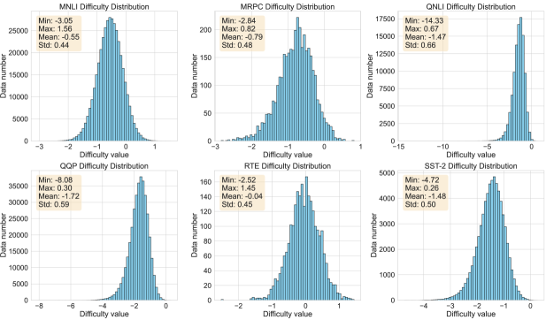
Figure 4: IRT-AC generated difficulty distribution on GLUE benchmark.

As illustrated in Figure 4, we present the difficulty distributions for examples in the GLUE benchmark datasets, as measured by IRT-AC. First, we observe that all distributions approximately follow a normal distribution. This observation meets our expectation that the majority of data points in GLUE tasks are neither too easy or too hard. Second, if we focus on the mean value of the difficulty, we can find that the QNLI, QQP, and SST-2 datasets exhibit the lowest mean difficulty values, suggesting that they are less challenging tasks. Conversely, the RTE dataset demonstrates a comparatively higher mean difficulty value, indicating it is a harder task than others in the GLUE. Importantly, these difficulty scores derived from IRT-AC demonstrate a strong correlation with empirical model performance. As the baseline results show in Table 4, we observe that tasks with lower mean difficulty values (QNLI, QQP, and SST-2) consistently yield higher accuracy scores. Conversely, the RTE task, characterized by a higher mean difficulty, results in the lowest accuracy among the GLUE tasks.

Artificial crowds’ accuracy on difficulty bin

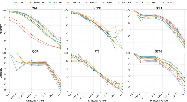
Figure 5: Accuracy of Artificial Crowds Using Various PLMs on the GLUE Benchmark. The legend indicates the PLMs utilized for creating the Artificial Crowds.

In this experiment, we aim to explore the accuracy of models in the AC on the GLUE benchmark. Specifically, we count the average percentage of correct responses for each model across different difficulty bins, ranging from $<-3$ (easiest) to $>3$ (hardest). As shown in Figure 5, we can observe a consistent difficulty trend: Across all tasks and models, there is a general downward trend in accuracy as the difficulty increases. Specifically, MNLI and QNLI show a gradual decline in accuracy across difficulty levels, suggesting a well-distributed range of challenge in these tasks. QQP and SST-2 maintain relatively high accuracy until the highest difficulty bins, indicating that these tasks may have a lower proportion of very challenging examples. RTE exhibits a steeper decline in accuracy, particularly in the mid-range difficulties, highlighting its overall challenging nature. MRPC shows more variability across models, especially in higher difficulty ranges, suggesting that this task may be particularly sensitive to model architecture differences. This consistent behavior validates IRT-AC in meaningfully quantifying task difficulty.

Confidence of the generated Difficulty

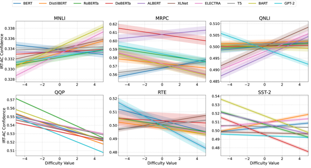
Figure 6: Artificial crowds’ confidence on GLUE. We use the probability of the correct label as the confidence metric.

In this next analysis, we seek to investigate the confidence levels of the artificial crowd models in their predicted results. Specifically, we utilize the logit function’s output for the correct label as a metric of AC model confidence. To visualize and analyze this confidence across different difficulty levels, we employ a linear regression with standard deviation to fit these results. As shown in Figure 6, we present the IRT-AC confidence trends across GLUE benchmark tasks for the artificial crowds. The figure reveals several intriguing patterns. Each GLUE task exhibits distinct confidence patterns across difficulty levels, suggesting that model confidence is highly task-dependent. Different artificial crowds show varying confidence trends, indicating that architecture plays a crucial role in how models assess their own certainty. In most tasks, there is a general trend of decreasing confidence as difficulty increases, albeit with some exceptions.

6 Conclusion

In this paper, we introduce PUDF, a novel Psychology-based Unified Framework for CL in fine-tuning pre-trained language models. By combining IRT-AC for data difficulty measurement and DDS-MAE for dynamic training scheduling, PUDF offers a theoretically grounded and automated approach to CL. Our extensive experiments on GLUE benchmark demonstrate that PUDF consistently improves both accuracy and training efficiency across multiple pre-trained language models and tasks, outperforming SOTA CL methods. The success of PUDF opens up promising directions for future research, including applications in other domains, such as computer vision and multimodal domains.

This work validates and supports the existing literature on curriculum learning. Our results confirm that curriculum learning frameworks for supervised learning can lead to faster convergence or better local minima, as measured by test set performance (Bengio et al., 2009). We have shown that by replacing a heuristic for difficulty with a theoretically-based, learned difficulty value for training examples, static curriculum learning frameworks can be improved. Probing the model’s ability allows for data to be selected for training that is appropriate for the model and is not rigidly tied to a heuristic schedule.

By using PUDF, a curriculum can adapt during training according to the estimated ability of the model. PUDF adds or removes training data based not on a fixed step schedule but rather by probing the model at each epoch and using the estimated ability to match data to the model. This way if a model has a high estimated ability early in training, then more data can be added to the training set more quickly and learning isn’t artificially slowed down due to the curriculum schedule. For each data set in question, PUDF adds training data more quickly than a more traditional curriculum learning schedule, which leads to faster convergence. It also allows for the possibility of a smaller dataset at later stages, if model performance decreases.

6.1 Limitations

One potential issue with PUDF is the chance of a high variance model, due to the additional step of estimating model ability during training. However, in our results we find that variance in terms of output performance is quite low for PUDF(Section 5.2). We can infer that the ability estimation process is relatively stable. That is, the example difficulties estimated from IRT are stable enough that ability estimates align with the current state of the model, as indicated by the regular progression through the curriculum and increasing training and validation accuracy performance. Our results show that adding this step does not lead to a higher variance model and, in certain cases, PUDF has lower variance than the baseline and competency-based frameworks.

For PUDF, there is a potentially significant cost associated with estimating $\theta_{e}$. Estimating $\theta_{e}$ requires an additional forward pass through the training data set to gather the labels for scoring as well as MLE estimation. For large data sets, this can effectively double the number of forward passes during training. To alleviate the extra cost, we sample from the training set before our first epoch, and use this down-sampled subset as our ability estimation set. As most examples have difficulty values between $-3$ and $3$, the full training set isn’t necessary for estimating $\theta_{e}$. Identifying the optimal number of examples needed to estimate ability is left for future work.

6.2 Future Work

Even though it is dynamic, PUDF employs a simple curriculum schedule: only include examples where difficulty is less than estimated ability. However, being able to estimate ability on the fly with PUDF opens up as a research area the following: what is the best way to build a curriculum, knowing example difficulty and model ability (e.g., the 85% rule of (Wilson et al., 2019))? It may be the case that only data with difficulty within a range of ability (higher and lower) is better, and the training set shifts as the model improves. There are many directions to for future work, and this will be an exciting area of work moving forward.

PUDF can also be adapted to more traditional information retrieval tasks, such as learning to rank (L2R) and online judging (OJ) for training high-ability systems and ordering examples according to learned difficulty. In particular, with a Rasch model, the intuitive link between $\theta$ and $b$ allows for inherently explainable training mechanisms. An example is only included in training if its difficulty is lower than the model’s estimated ability at that point in time. This can be easily explained to model stakeholders and compared with standardized tests for humans, where questions are selected based on human estimated ability. It may be the case that only data with difficulty within a range of ability (higher and lower) is better, and the training set shifts as the model improves.

Appendix A Appendix

A.1 Original Formulation of Artificial Crowd

Figure 7: Response pattern construction for IRT model fitting with artificial crowds.

A.2 Additional qualitative analysis on IRT-AC

Here we replicate the qualitative analysis discussed in Section 5.5 for the other datasets in GLUE. These examples provide further insights into the IRT-AC on other datasets of GLUE benchmark by presenting the top 5 hardest and easiest sentences for each dataset, along with their respective labels and difficulty scores.

Table 9: Top 5 Hardest and Easiest Sentences in MNLI.

Hardest Sentence	Label	Difficulty	Easiest Sentence	Label	Difficulty
#1a but we do don’t we	1	1.539	#1a uh-huh right and so we we have really enjoyed that and it’s really nice not to be running out some of the video rentals can be expensive and	2	-3.044
#1b We probably do			#1b I would never rent a movie.
#2a The hotel price categories below are based on regular-season rates for a standard double room, excluding a 15 percent service charge.	0	1.389	#2a But at least it came on a nice paper plate.	0	-2.944
#2b The hotel has prices lower than the regular season rates.			#2b It was served on a nice paper plate.
#3a Further, Passaic charges that LSNJ is breaching a fiduciary duty owed to local programs by competing with them for money to fund its own programs.	0	1.370	#3a She closed her eyes and Jon’s vision expanded.	2	-2.813
#3b LSNJ is being accused of breaking a judiciary duty.			#3b When she closed her eye no one was able to see.
#4a Definitional Creep?	1	1.326	#4a James Mason and Orson Welles began their acting careers here.	2	-2.777
#4b The teacher wanted the students to find the definition of creep.			#4b Orson Welles never acted here.
#5a Today, the Loire is a sleepy waterway, running deep only with heavy rains or spring thaws, and its sandbanks and mud flats become islands during the summer.	1	1.319	#5a that’s where the only stipulation i’d like to see tacked on to the legislation saying that there had to be some form of formal firearms instruction N R say NRA certified firearms instruction	2	-2.765
#5b The Loire is met with frequent rain throughout the seasons.			#5b The NRA should not be trusted with firearms instruction.

Table 10: Top 5 Hardest and Easiest Sentences in MRPC.

Hardest Sentence	Label	Difficulty	Easiest Sentence	Label	Difficulty
#1a They looked at their son-in-law and his relatives, but did not exchange words.	1	0.859	#1a The Dow Jones Industrial Average ended down 128 points, or 1.4%, at 9073, while the Nasdaq fell 34 points, or 2.1%, to 1610.	0	-2.686
#1b She looked at her son-in-law and his relatives at times, but the two sides did not exchange words.			#1b In early trading, the Dow Jones industrial average was up 3.90, or 0.04 percent, at 9,113.75, having gained 36.90 on Tuesday.
#2a They found molecules that can only be produced when ozone breaks down cholesterol.	1	0.558	#2a That means that if the planet is in a season, it will continue to brighten for the next 20 years.	1	-2.674
#2b And all of the samples contained molecules that can only be produced when cholesterol interacts with ozone.			#2b If what scientists are observing is truly seasonal change, the planet will continue to brighten for another 20 years.
#3a Take-Two also defended its right to create a ”realistic” game for an adult audience.	1	0.549	#3a Germany’s Foreign Ministry said it believed the passengers were from the northern states of Lower Saxony and Schleswig-Holstein, but had no further details.	0	-2.638
#3b The company also defended its right to ”create a video game experience with a certain degree of realism.”			#3b Germany said most of the passengers were from the northern states of Lower Saxony and Schleswig-Holstein.
#4a The ELF has claimed responsibility for a slew of arson attacks against commercial entities that members say threaten or damage the environment.	1	0.472	#4a Branch was later fired by the company and eventually filed a wrongful-termination suit that included details about the documents, the Journal story said.	0	-2.608
#4b The underground group has claimed responsibility for a series of arsons against commercial entities that members say damage the environment.			#4b The former employees filed wrongful-termination suits, dismissed in July 2002, that included details about the documents, the Journal story said.
#5a Viacom’s lawyers say Spike is a common name that does not necessarily prompt thoughts of Lee.	1	0.472	#5a He said that President Bush’s proposed Clean Air Act amendment, called the Clear Skies Initiative, would result in greater efficiency and therefore less pollution.	0	-2.588
#5b Viacom’s lawyers say Spike is a common name that doesn’t necessarily prompt thoughts of the 46-year-old film director.			#5b He said that by allowing power companies more flexibility, the Clear Skies Initiative would result in greater efficiency and therefore less pollution.

Table 11: Top 5 Hardest and Easiest Sentences in QNLI.

Hardest Sentence	Label	Difficulty	Easiest Sentence	Label	Difficulty
#1a Humoral immunology theorized that the origin of the immune system lay in what?	1	0.637	#1a What was the name of the local government and tribunal?	0	-14.401
#1b Many theories have been suggested in immunology from the end of the nineteenth century up to the present time.			#1b These reforms, while establishing a local government and tribunal (the Real Audiencia del Reino de Galicia) and bringing the nobleman under submission, also brought most Galician monasteries and institutions under Castilian control, in what has been criticized as a process of centralisation.
#2a Which U.S. Billboard 200 chart topper did Kanye West produce a song for?	1	0.585	#2a Is I-91 similar to I-95 in terms of bad traffic?	0	-11.581
#2b Her second effort subsequently became the very first hip-hop album by a female rapper to debut at the top of the U.S. Billboard 200 chart in its first week of release.			#2b I-95 is infamous for traffic jams increasing with proximity to New York City; on the east side of New Haven it passes over the Quinnipiac River via the Pearl Harbor Memorial, or ”Q Bridge”, which often presents a major bottleneck to traffic. I-91, however, is relatively less congested, except at the intersection with I-95 during peak travel times.
#3a What two neighborhoods are the centers of the quartiers sensibles?	1	0.542	#3a Who did Nasser imprison thousands of?	0	-10.446
#3b To the north of the city they are grouped mainly in the Seine-Saint-Denis department, and to a lesser extreme to the east in the Val-d’Oise department.			#3b Nasser’s Egyptian detractors considered him a dictator who thwarted democratic progress, imprisoned thousands of dissidents, and led a repressive administration responsible for numerous human rights violations.
#4a Why do mountain and moorland breeders move only altitudinally?	1	0.394	#4a What act calls for 7.5 billion US gallons of biofuels to be used annually by 2012?	0	-8.299
#4b Species like the chaffinch are much less migratory in Britain than those of continental Europe, mostly not moving more than 5 km in their lives.			#4b The Energy Policy Act of 2005, which calls for 7.5 billion US gallons (28,000,000 m3) of biofuels to be used annually by 2012, will also help to expand the market.
#5a How much of the population did Prussia control?	1	0.393	#5a What park hosts Quarter horse racing?	0	-8.217
#5b The Confederation was dissolved after the Austro-Prussian War and replaced by a North German Federation under Prussian hegemony; this war left Prussia dominant in Germany, and German nationalism would compel the remaining independent states to ally with Prussia in the Franco-Prussian War of 1870–71, and then to accede to the crowning of King Wilhelm of Prussia as German Emperor.			#5b Other major sporting events include Thoroughbred and Quarter horse racing circuits at Remington Park and numerous horse shows and equine events that take place at the state fairgrounds each year.

Table 12: Top 5 Hardest and Easiest Sentences in QQP.

Hardest Sentence	Label	Diff.	Easiest Sentence	Label	Diff.
#1a How will I get a government engineering job after completing my mechanical engineering?	0	0.313	#1a Which university is best in Germany for doing MS in Computer Science?	1	-8.086
#1b How will I get a government engineering job after completing my electrical engineering?			#1b What are some good universities in Germany for masters in computer science?
#2a In which Star Wars film does Darth Vader first have his helmet off?	0	0.257	#2a How can I excel as a physician?	1	-7.617
#2b ”Why did Darth Bane die in ””Star Wars”” book?”			#2b How can I be an excellent physician?
#3a What are some good mosquito repellents for dogs?	0	0.244	#3a What is the best free web hosting service/site?	1	-7.472
#3b Which is the best mosquito repeller?			#3b I need a free web hosting for my blog, what is the best free web hosting?
#4a What are the functions of stock exchange?	0	0.234	#4a What is a good minor that will compliment a Computer Science major?	1	-7.301
#4b How do stock exchanges function?			#4b What is the best minor for Computer Science Majors?
#5a What is the formula to calculate millimolar? How is this formula determined?	0	0.220	#5a What are the best books on coaching?	1	-7.091
#5b What is the formula of methene? How is it determined?			#5b What are some good books for coaching?

Table 13: Top 5 Hardest and Easiest Sentences in RTE.

Hardest Sentence	Label	Difficulty	Easiest Sentence	Label	Difficulty
#1a During a IRS raid in Spring 2006, the government confiscated records, $42,000 in cash was seized, and that day Kent Hovind withdrew $70,000 from the Creation Science Evangelism account, half in a check; the other in cash. At the November trial, the young Earth creationist chose not to present a defense case. While the prosecution noted Hovind never filed income taxes with the government, others testified Hovind claimed he had ”beat” the tax system, and employees said Hovind’s evangelism was a business not a ministry.	1	1.375	#1a Coal company stocks got a lift Monday morning after an article in Barron’s said the industry was benefiting from soaring natural gas prices and the advent of new power plants that emit less pollution.	0	-2.536
#1b Hovind was found guilty on 59 federal counts.			#1b Coal stocks rise.
#2a I have a 1986 Coca-Cola Grand Union 100 Year Statue of Liberty pin set.	1	1.362	#2a Mossad is one of the world’s most well-known intelligence agencies, and is often viewed in the same regard as the CIA and MI6.	0	-1.640
#2b The Statue of Liberty was built in 1986.			#2b Mossad is an intelligence agency.
#3a Muslims are commanded not to take Jews or Christians for friends.	1	1.323	#3a ”How come a country (Vatican City), a so-called country, that is in essence 800 square acres of office space in the middle of Rome, that has a citizenry that excludes women and children, seems to attract the most attention in talking about public policy that deals with women and children?” she demanded.	0	-1.612
#3b Jews and Christians pray as Muslims do.			#3b The Vatican City is in Rome.
#4a Manuel Rosales, who ran against Mr Chavez in the 2006 presidential election, faces corruption charges he says are baseless. He had been in hiding since the charges were filed last month. Venezuela’s Interior Minister Tareck el-Aissami said Mr Rosales was a criminal on the run. ”If he doesn’t appear before the appropriate courts, he would be a fugitive from justice, and as a result the court will activate mechanisms for his international capture,” said Mr Aissami, denying that the charges were political.	1	1.299	#4a In the glamorous, exclusive world of French haute couture, Sakina M’Sa is an unlikely star. Like her creations, M’Sa is the sum of many parts - a tiny woman from the Comoros, an immigrant from a working-class neighbourhood in Marseille, and a designer who follows her own dreams and embroiders the fashion world with a social conscience. ”My only strength in life is my difference,” says M’Sa, dressed all in black and sitting in her workshop and showroom in La Goutte d’Or, a working-class neighbourhood in Paris which is home to a large population of Africans.	0	-1.609
#4b Manuel Rosales was mayor of Maracaibo.			#4b Sakina M’Sa has Comoros origins.
#5a Every year, about a quarter of all children sustain an injury serious enough to require medical attention, school absences, and/or bed rest.	1	1.292	#5a Sotheby’s and Christie’s, the world’s two most powerful auction houses, swapped confidential lists of super-rich clients who were spared from paying fees charged to other sellers, people close to the companies and to a federal antitrust investigation of them said.	0	-1.599
#5b Fireworks may cause serious injuries.			#5b Christie’s is one of the world’s largest auction houses.

References

- (1)
- Bai et al. (2022) Ziwei Bai, Junpeng Liu, Meiqi Wang, Caixia Yuan, and Xiaojie Wang. 2022. Exploiting diverse information in pre-trained language model for multi-choice machine reading comprehension. Applied Sciences 12, 6 (2022), 3072.
- Baker and Kim (2004) Frank B. Baker and Seock-Ho Kim. 2004. Item Response Theory: Parameter Estimation Techniques, Second Edition. CRC Press.
- Bengio et al. (2009) Yoshua Bengio, Jérôme Louradour, Ronan Collobert, and Jason Weston. 2009. Curriculum learning. In Proceedings of the 26th annual international conference on machine learning. ACM, 41–48. http://dl.acm.org/citation.cfm?id=1553380
- Bentivogli et al. (2009) Luisa Bentivogli, Ido Dagan, Hoa Trang Dang, Danilo Giampiccolo, and Bernardo Magnini. 2009. The Fifth PASCAL Recognizing Textual Entailment Challenge. In Proceedings of the Text Analysis Conference (TAC).
- Bingham et al. (2018) Eli Bingham, Jonathan P. Chen, Martin Jankowiak, Fritz Obermeyer, Neeraj Pradhan, Theofanis Karaletsos, Rohit Singh, Paul Szerlip, Paul Horsfall, and Noah D. Goodman. 2018. Pyro: Deep Universal Probabilistic Programming. Journal of Machine Learning Research (2018).
- Bock and Aitkin (1981) R Darrell Bock and Murray Aitkin. 1981. Marginal maximum likelihood estimation of item parameters: Application of an EM algorithm. Psychometrika 46, 4 (1981), 443–459.
- Bowman et al. (2015) Samuel Bowman, Gabor Angeli, Christopher Potts, and Christopher D Manning. 2015. A large annotated corpus for learning natural language inference. In Proceedings of the 2015 Conference on Empirical Methods in Natural Language Processing. 632–642.
- Brown et al. (2020) Tom Brown, Benjamin Mann, Nick Ryder, Melanie Subbiah, Jared D Kaplan, Prafulla Dhariwal, Arvind Neelakantan, Pranav Shyam, Girish Sastry, Amanda Askell, et al. 2020. Language models are few-shot learners. Advances in neural information processing systems 33 (2020), 1877–1901.
- Burduja and Ionescu (2021) Mihail Burduja and Radu Tudor Ionescu. 2021. Unsupervised medical image alignment with curriculum learning. In 2021 IEEE International Conference on Image Processing (ICIP). IEEE, 3787–3791.
- Cer et al. (2017) Daniel Cer, Mona Diab, Eneko Agirre, Inigo Lopez-Gazpio, and Lucia Specia. 2017. Semeval-2017 task 1: Semantic textual similarity-multilingual and cross-lingual focused evaluation. arXiv preprint arXiv:1708.00055 (2017).
- Cirik et al. (2016) Volkan Cirik, Eduard Hovy, and Louis-Philippe Morency. 2016. Visualizing and understanding curriculum learning for long short-term memory networks. arXiv preprint arXiv:1611.06204 (2016).
- Clark et al. (2020) Kevin Clark, Minh-Thang Luong, Quoc V Le, and Christopher D Manning. 2020. Electra: Pre-training text encoders as discriminators rather than generators. arXiv preprint arXiv:2003.10555 (2020).
- De Ayala (2013) Rafael Jaime De Ayala. 2013. The theory and practice of item response theory. Guilford Publications.
- Dolan and Brockett (2005) William B Dolan and Chris Brockett. 2005. Automatically constructing a corpus of sentential paraphrases. In Proceedings of the International Workshop on Paraphrasing.
- Elman (1993) Jeffrey L Elman. 1993. Learning and development in neural networks: The importance of starting small. Cognition 48, 1 (1993), 71–99.
- Freund and Schapire (1997) Yoav Freund and Robert E Schapire. 1997. A decision-theoretic generalization of on-line learning and an application to boosting. Journal of computer and system sciences 55, 1 (1997), 119–139.
- Graves et al. (2017) Alex Graves, Marc G Bellemare, Jacob Menick, Remi Munos, and Koray Kavukcuoglu. 2017. Automated curriculum learning for neural networks. In international conference on machine learning. Pmlr, 1311–1320.
- Guo et al. (2022) Shangwei Guo, Chunlong Xie, Jiwei Li, Lingjuan Lyu, and Tianwei Zhang. 2022. Threats to pre-trained language models: Survey and taxonomy. arXiv preprint arXiv:2202.06862 (2022).
- Hacohen and Weinshall (2019) Guy Hacohen and Daphna Weinshall. 2019. On the power of curriculum learning in training deep networks. In International conference on machine learning. PMLR, 2535–2544.
- He et al. (2022) Pengcheng He, Jianfeng Gao, and Weizhu Chen. 2022. DeBERTaV3: Improving DeBERTa using ELECTRA-Style Pre-Training with Gradient-Disentangled Embedding Sharing. In The Eleventh International Conference on Learning Representations.
- He et al. (2020) Pengcheng He, Xiaodong Liu, Jianfeng Gao, and Weizhu Chen. 2020. Deberta: Decoding-enhanced bert with disentangled attention. arXiv preprint arXiv:2006.03654 (2020).
- Hoffman et al. (2013) Matthew D Hoffman, David M Blei, Chong Wang, and John Paisley. 2013. Stochastic variational inference. Journal of Machine Learning Research (2013).
- Jiang et al. (2015) Lu Jiang, Deyu Meng, Qian Zhao, Shiguang Shan, and Alexander Hauptmann. 2015. Self-paced curriculum learning. In Proceedings of the AAAI Conference on Artificial Intelligence, Vol. 29.
- Jordan et al. (1999) Michael I Jordan, Zoubin Ghahramani, Tommi S Jaakkola, and Lawrence K Saul. 1999. An introduction to variational methods for graphical models. Machine learning 37 (1999), 183–233.
- Kalyan et al. (2021) Katikapalli Subramanyam Kalyan, Ajit Rajasekharan, and Sivanesan Sangeetha. 2021. Ammus: A survey of transformer-based pretrained models in natural language processing. arXiv preprint arXiv:2108.05542 (2021).
- Kenton and Toutanova (2019) Jacob Devlin Ming-Wei Chang Kenton and Lee Kristina Toutanova. 2019. BERT: Pre-training of Deep Bidirectional Transformers for Language Understanding. In Proceedings of NAACL-HLT. 4171–4186.
- Khan et al. (2022) Salman Khan, Muzammal Naseer, Munawar Hayat, Syed Waqas Zamir, Fahad Shahbaz Khan, and Mubarak Shah. 2022. Transformers in vision: A survey. ACM computing surveys (CSUR) 54, 10s (2022), 1–41.
- Kocmi and Bojar (2017) Tom Kocmi and Ondřej Bojar. 2017. Curriculum Learning and Minibatch Bucketing in Neural Machine Translation. In Proceedings of the International Conference Recent Advances in Natural Language Processing, RANLP 2017. 379–386.
- Kumar et al. (2019) Gaurav Kumar, George Foster, Colin Cherry, and Maxim Krikun. 2019. Reinforcement learning based curriculum optimization for neural machine translation. arXiv preprint arXiv:1903.00041 (2019).
- Kumar et al. (2010) M Kumar, Benjamin Packer, and Daphne Koller. 2010. Self-paced learning for latent variable models. Advances in neural information processing systems 23 (2010).
- Lagarias et al. (1998) Jeffrey C Lagarias, James A Reeds, Margaret H Wright, and Paul E Wright. 1998. Convergence properties of the Nelder–Mead simplex method in low dimensions. SIAM Journal on optimization 9, 1 (1998), 112–147.
- Lalor and Rodriguez (2023) John Patrick Lalor and Pedro Rodriguez. 2023. py-irt: A scalable item response theory library for python. INFORMS Journal on Computing 35, 1 (2023), 5–13.
- Lalor et al. (2019) John P. Lalor, Hao Wu, and Hong Yu. 2019. Learning Latent Parameters without Human Response Patterns: Item Response Theory with Artificial Crowds. In Proceedings of the Conference on Empirical Methods in Natural Language Processing. Conference on Empirical Methods in Natural Language Processing, Vol. 2019. Association for Computational Linguistics.
- Lalor and Yu (2020) John P. Lalor and Hong Yu. 2020. Dynamic Data Selection for Curriculum Learning via Ability Estimation. In Findings of the Association for Computational Linguistics: EMNLP 2020. Association for Computational Linguistics, Online, 545–555. https://doi.org/10.18653/v1/2020.findings-emnlp.48
- Lan et al. (2019) Zhenzhong Lan, Mingda Chen, Sebastian Goodman, Kevin Gimpel, Piyush Sharma, and Radu Soricut. 2019. Albert: A lite bert for self-supervised learning of language representations. arXiv preprint arXiv:1909.11942 (2019).
- Lewis et al. (2019) Mike Lewis, Yinhan Liu, Naman Goyal, Marjan Ghazvininejad, Abdelrahman Mohamed, Omer Levy, Ves Stoyanov, and Luke Zettlemoyer. 2019. Bart: Denoising sequence-to-sequence pre-training for natural language generation, translation, and comprehension. arXiv preprint arXiv:1910.13461 (2019).
- Liu et al. (2022) Fenglin Liu, Shen Ge, Yuexian Zou, and Xian Wu. 2022. Competence-based multimodal curriculum learning for medical report generation. arXiv preprint arXiv:2206.14579 (2022).
- Liu et al. (2019) Yinhan Liu, Myle Ott, Naman Goyal, Jingfei Du, Mandar Joshi, Danqi Chen, Omer Levy, Mike Lewis, Luke Zettlemoyer, and Veselin Stoyanov. 2019. Roberta: A robustly optimized bert pretraining approach. arXiv preprint arXiv:1907.11692 (2019).
- Loshchilov et al. (2017) Ilya Loshchilov, Frank Hutter, et al. 2017. Fixing weight decay regularization in adam. arXiv preprint arXiv:1711.05101 5 (2017).
- Maharana and Bansal (2022) Adyasha Maharana and Mohit Bansal. 2022. On curriculum learning for commonsense reasoning. In Proceedings of the 2022 Conference of the North American Chapter of the Association for Computational Linguistics: Human Language Technologies. 983–992.
- Manela and Biess (2022) Binyamin Manela and Armin Biess. 2022. Curriculum learning with hindsight experience replay for sequential object manipulation tasks. Neural Networks 145 (2022), 260–270.
- Matiisen et al. (2019) Tambet Matiisen, Avital Oliver, Taco Cohen, and John Schulman. 2019. Teacher–student curriculum learning. IEEE transactions on neural networks and learning systems 31, 9 (2019), 3732–3740.
- Milano and Nolfi (2021) Nicola Milano and Stefano Nolfi. 2021. Automated curriculum learning for embodied agents a neuroevolutionary approach. Scientific reports 11, 1 (2021), 8985.
- Mohiuddin et al. (2022) Tasnim Mohiuddin, Philipp Koehn, Vishrav Chaudhary, James Cross, Shruti Bhosale, and Shafiq Joty. 2022. Data Selection Curriculum for Neural Machine Translation. In Findings of the Association for Computational Linguistics: EMNLP 2022, Yoav Goldberg, Zornitsa Kozareva, and Yue Zhang (Eds.). Association for Computational Linguistics, Abu Dhabi, United Arab Emirates, 1569–1582. https://doi.org/10.18653/v1/2022.findings-emnlp.113
- Natesan et al. (2016) Prathiba Natesan, Ratna Nandakumar, Tom Minka, and Jonathan D. Rubright. 2016. Bayesian Prior Choice in IRT Estimation Using MCMC and Variational Bayes. Frontiers in Psychology 7 (Sept. 2016). https://doi.org/10.3389/fpsyg.2016.01422
- Ouyang et al. (2023) Jihong Ouyang, Zhiyao Yang, Chang Xuan, Bing Wang, Yiyuan Wang, and Ximing Li. 2023. Unsupervised Aspect Term Extraction by Integrating Sentence-level Curriculum Learning with Token-level Self-paced Learning. In Proceedings of the 32nd ACM International Conference on Information and Knowledge Management. 1982–1991.
- Platanios et al. (2019) Emmanouil Antonios Platanios, Otilia Stretcu, Graham Neubig, Barnabas Poczos, and Tom Mitchell. 2019. Competence-based Curriculum Learning for Neural Machine Translation. In Proceedings of the 2019 Conference of the North American Chapter of the Association for Computational Linguistics: Human Language Technologies, Volume 1 (Long and Short Papers). Association for Computational Linguistics, Minneapolis, Minnesota, 1162–1172. https://www.aclweb.org/anthology/N19-1119
- Radford et al. (2019) Alec Radford, Jeff Wu, Rewon Child, David Luan, Dario Amodei, and Ilya Sutskever. 2019. Language Models are Unsupervised Multitask Learners. Technical Report. OpenAI.
- Raffel et al. (2020) Colin Raffel, Noam Shazeer, Adam Roberts, Katherine Lee, Sharan Narang, Michael Matena, Yanqi Zhou, Wei Li, and Peter J. Liu. 2020. Exploring the Limits of Transfer Learning with a Unified Text-to-Text Transformer. Journal of Machine Learning Research 21, 140 (2020), 1–67. http://jmlr.org/papers/v21/20-074.html
- Rajpurkar et al. (2016) Pranav Rajpurkar, Jian Zhang, Konstantin Lopyrev, and Percy Liang. 2016. SQuAD: 100,000+ Questions for Machine Comprehension of Text. In Proceedings of EMNLP (Austin, Texas). Association for Computational Linguistics, 2383–2392.
- Rasch (1960) Georg Rasch. 1960. Studies in mathematical psychology: I. Probabilistic models for some intelligence and attainment tests. Nielsen & Lydiche, Oxford, England.
- Rodriguez et al. (2021) Pedro Rodriguez, Joe Barrow, Alexander Miserlis Hoyle, John P Lalor, Robin Jia, and Jordan Boyd-Graber. 2021. Evaluation examples are not equally informative: How should that change NLP leaderboards?. In Proceedings of the 59th Annual Meeting of the Association for Computational Linguistics and the 11th International Joint Conference on Natural Language Processing (Volume 1: Long Papers). 4486–4503.
- Sanh et al. (2019) Victor Sanh, Lysandre Debut, Julien Chaumond, and Thomas Wolf. 2019. DistilBERT, a distilled version of BERT: smaller, faster, cheaper and lighter. arXiv preprint arXiv:1910.01108 (2019).
- Sengupta et al. (2023) Ayan Sengupta, Shantanu Dixit, Md Shad Akhtar, and Tanmoy Chakraborty. 2023. A Good Learner can Teach Better: Teacher-Student Collaborative Knowledge Distillation. In The Twelfth International Conference on Learning Representations.
- Shrivastava et al. (2016) Abhinav Shrivastava, Abhinav Gupta, and Ross Girshick. 2016. Training region-based object detectors with online hard example mining. In Proceedings of the IEEE conference on computer vision and pattern recognition. 761–769.
- Socher et al. (2013) Richard Socher, Alex Perelygin, Jean Wu, Jason Chuang, D. Christopher Manning, Andrew Ng, and Christopher Potts. 2013. Recursive Deep Models for Semantic Compositionality Over a Sentiment Treebank. In Proceedings of the 2013 Conference on Empirical Methods in Natural Language Processing. Association for Computational Linguistics, Seattle, Washington, USA, 1631–1642. http://aclweb.org/anthology/D13-1170
- Soviany et al. (2021) Petru Soviany, Radu Tudor Ionescu, Paolo Rota, and Nicu Sebe. 2021. Curriculum self-paced learning for cross-domain object detection. Computer Vision and Image Understanding 204 (2021), 103166.
- Spitkovsky et al. (2010) Valentin I Spitkovsky, Hiyan Alshawi, and Dan Jurafsky. 2010. From baby steps to leapfrog: How “less is more” in unsupervised dependency parsing. In Human Language Technologies: The 2010 Annual Conference of the North American Chapter of the Association for Computational Linguistics. 751–759.
- Tay et al. (2022) Yi Tay, Mostafa Dehghani, Dara Bahri, and Donald Metzler. 2022. Efficient Transformers: A Survey. ACM Comput. Surv. 55, 6, Article 109 (dec 2022), 28 pages. https://doi.org/10.1145/3530811
- Tsvetkov et al. (2016) Yulia Tsvetkov, Manaal Faruqui, Wang Ling, Brian MacWhinney, and Chris Dyer. 2016. Learning the Curriculum with Bayesian Optimization for Task-Specific Word Representation Learning. In Proceedings of the 54th Annual Meeting of the Association for Computational Linguistics (Volume 1: Long Papers). 130–139.
- Vaswani et al. (2017) Ashish Vaswani, Noam Shazeer, Niki Parmar, Jakob Uszkoreit, Llion Jones, Aidan N Gomez, Łukasz Kaiser, and Illia Polosukhin. 2017. Attention is all you need. Advances in neural information processing systems 30 (2017).
- Wan et al. (2020) Yu Wan, Baosong Yang, Derek F. Wong, Yikai Zhou, Lidia S. Chao, Haibo Zhang, and Boxing Chen. 2020. Self-Paced Learning for Neural Machine Translation. In Proceedings of the 2020 Conference on Empirical Methods in Natural Language Processing (EMNLP), Bonnie Webber, Trevor Cohn, Yulan He, and Yang Liu (Eds.). Association for Computational Linguistics, Online, 1074–1080. https://doi.org/10.18653/v1/2020.emnlp-main.80
- Wang et al. (2019) Alex Wang, Amanpreet Singh, Julian Michael, Felix Hill, Omer Levy, and Samuel R. Bowman. 2019. GLUE: A Multi-Task Benchmark and Analysis Platform for Natural Language Understanding. In Proceedings of the International Conference on Learning Representations (ICLR).
- Wang et al. (2021) Xin Wang, Yudong Chen, and Wenwu Zhu. 2021. A survey on curriculum learning. IEEE transactions on pattern analysis and machine intelligence 44, 9 (2021), 4555–4576.
- Wei et al. (2016) Yunchao Wei, Xiaodan Liang, Yunpeng Chen, Xiaohui Shen, Ming-Ming Cheng, Jiashi Feng, Yao Zhao, and Shuicheng Yan. 2016. Stc: A simple to complex framework for weakly-supervised semantic segmentation. IEEE transactions on pattern analysis and machine intelligence 39, 11 (2016), 2314–2320.
- Weinshall et al. (2018) Daphna Weinshall, Gad Cohen, and Dan Amir. 2018. Curriculum learning by transfer learning: Theory and experiments with deep networks. In International conference on machine learning. PMLR, 5238–5246.
- Williams et al. (2018) Adina Williams, Nikita Nangia, and Samuel R. Bowman. 2018. A Broad-Coverage Challenge Corpus for Sentence Understanding through Inference. In Proceedings of NAACL-HLT.
- Wilson et al. (2019) Robert C. Wilson, Amitai Shenhav, Mark Straccia, and Jonathan D. Cohen. 2019. The Eighty Five Percent Rule for Optimal Learning. Nature Communications (2019). https://doi.org/10.1038/s41467-019-12552-4
- Wu et al. (2020) Mike Wu, Richard L. Davis, Benjamin W. Domingue, Chris Piech, and Noah D. Goodman. 2020. Variational Item Response Theory: Fast, Accurate, and Expressive. In Proceedings of the 13th International Conference on Educational Data Mining, EDM 2020, Fully virtual conference, July 10-13, 2020, Anna N. Rafferty, Jacob Whitehill, Cristóbal Romero, and Violetta Cavalli-Sforza (Eds.). International Educational Data Mining Society. https://educationaldatamining.org/files/conferences/EDM2020/papers/paper_22.pdf
- Xu et al. (2020) Benfeng Xu, Licheng Zhang, Zhendong Mao, Quan Wang, Hongtao Xie, and Yongdong Zhang. 2020. Curriculum learning for natural language understanding. In Proceedings of the 58th Annual Meeting of the Association for Computational Linguistics. 6095–6104.
- Yang et al. (2019) Zhilin Yang, Zihang Dai, Yiming Yang, Jaime Carbonell, Russ R Salakhutdinov, and Quoc V Le. 2019. Xlnet: Generalized autoregressive pretraining for language understanding. Advances in neural information processing systems 32 (2019).
- Yao et al. (2007) Yuan Yao, Lorenzo Rosasco, and Andrea Caponnetto. 2007. On early stopping in gradient descent learning. Constructive Approximation 26, 2 (2007), 289–315.
- Yuan et al. (2019) Xiaoyong Yuan, Pan He, Qile Zhu, and Xiaolin Li. 2019. Adversarial examples: Attacks and defenses for deep learning. IEEE transactions on neural networks and learning systems 30, 9 (2019), 2805–2824.
- Zhan et al. (2021) Runzhe Zhan, Xuebo Liu, Derek F Wong, and Lidia S Chao. 2021. Meta-curriculum learning for domain adaptation in neural machine translation. In Proceedings of the AAAI Conference on Artificial Intelligence, Vol. 35. 14310–14318.
- Zhang et al. (2021) Bowen Zhang, Yidong Wang, Wenxin Hou, Hao Wu, Jindong Wang, Manabu Okumura, and Takahiro Shinozaki. 2021. Flexmatch: Boosting semi-supervised learning with curriculum pseudo labeling. Advances in Neural Information Processing Systems 34 (2021), 18408–18419.
- Zhang et al. (2024) Shixing Zhang, Deqiang Han, Jean Dezert, and Yi Yang. 2024. Weighted Self-Paced Learning with Belief Functions. Expert Systems with Applications (2024), 124535.
- Zhao et al. (2020) Mingjun Zhao, Haijiang Wu, Di Niu, and Xiaoli Wang. 2020. Reinforced curriculum learning on pre-trained neural machine translation models. In Proceedings of the AAAI Conference on Artificial Intelligence, Vol. 34. 9652–9659.
- Zhao et al. (2021) Yangyang Zhao, Zhenyu Wang, and Zhenhua Huang. 2021. Automatic curriculum learning with over-repetition penalty for dialogue policy learning. In Proceedings of the AAAI Conference on Artificial Intelligence. 14540–14548.