Discrete-time immunization number

Abstract

We introduce a discrete-time immunization version of the SEIS compartment model of infection by a contagious disease, with an extended latency and protective period. The population is modeled by a graph $H$ where vertices represent individuals and edges exist between individuals with close connections. Our objective is to clear the population of infection while minimizing the maximum number of immunizations that occur at each time-step. We prove that this minimum is bounded above by a natural function of the pathwidth of $H$. In addition to our general results, we also focus on the case where the latency and protective periods last for one time-step. In this case, we characterize graphs that require only one immunization per time-step, provide a useful tool for proving lower bounds, and show that, for any tree $T$, there is a subdivision of $T$ that requires at most two immunizations per time-step.

1 Introduction

Infections can spread widely, and vaccinations against them, or therapeutic vaccinations for infected individuals, provide only time-limited immunity. Decisions about where to allocate immunizers and vaccinations are important in controlling outbreaks. Using graph theory, we introduce a new model of an infected population, with the goal of using the smallest possible number of immunizers to clear the infection. The population is the vertex set of a graph $H$, and each person is represented by a vertex of $H$. An edge in $H$ between two vertices $u$ and $v$ represents a close connection between the two people corresponding to $u$ and $v$. At the initial time-step, defined formally in the next paragraph, every vertex in $H$ is assumed to be infected. Our goal is to change every vertex to a non-infected state, using a minimum number of immunizers.

The three classes of members of the population in our model are healthy, infected (but not yet contagious), and contagious. This reflects the real-world protective period of many vaccines, as well as the latency period during which an infected individual is not contagious. Such classes as this are called compartments in Susceptible-Exposed-Infectious-Susceptible (SEIS) models of infection. These models are used to study epidemics and the spread of computer viruses. In our model, vaccination and contagion occur in discrete time-steps. At time 0, every vertex is contagious. At each discrete time-step $t\geq 1$, a group of vertices is vaccinated, and all of these vertices become healthy at time $t$. Every non-vaccinated vertex is exposed to all of its neighbors. A healthy vertex beyond the protective period with a contagious neighbor becomes infected, and an infected vertex becomes contagious after the latency period. Contagious vertices remain contagious until immunized. Figure 2 illustrates our model. Our goal is to construct an immunization protocol to transform all vertices in a graph to healthy ones.

SEIS compartment models have been well-studied using dynamic and stochastic processes. The point of view has generally been to analyze the number of people infected over time during an epidemic. Although a number of articles consider the spread of an epidemic on random graphs (see, for example, [10, 12, 13, 17] and [9] for history and an introduction), very few consider a deterministic discrete-time model. Recently, Figueiredo et al. [11] considered a discrete-time epidemic model on vertex-transitive graphs, complete graphs and some other graph families to find the epicenter of infection. It is a different model with a different goal than the one we use, but it is more similar in technique, because it uses discrete graph theory methods. There are many deterministic graph theoretic problems that involving changing the states of vertices in a graph over time, such as percolation, power domination, zero-forcing, graph burning, and graph cleaning. For more information on these models, see for example, [2, 8, 16, 18]. Our model and methods have commonalities with the study of the node search number of a graph. See [7, 14] for more on node searching.

Our work on the immunization number in this paper were inspired by an open problem regarding the inspection game, presented by A. Bernshteyn at the Graph Theory Workshop at Dawson College (Québec) in June 2023. In the inspection game [1], an invisible intruder initially chooses a vertex to occupy. At each step, searchers “inspect” a set of $k$ vertices. If the intruder occupies one of the inspected vertices, the game ends and the searcher wins. Otherwise, the intruder can secretly choose to move to an adjacent vertex or (secretly) remain at the same vertex. The inspection number of a graph is the minimum $k$ such that the game ends after a finite sequence of steps. Following the terminology of traditional searching models for invisible intruders, the inspection problem can also be equivalently formulated in terms of searchers aiming to clear vertices of a contaminant. That is, during each round, the searchers “clear” a set of $k$ vertices of the contaminant and then every cleared vertex that has a contaminated neighbor becomes contaminated again. A search strategy is monotonic if recontamination does not occur. The inspection number of a graph is less than or equal to one plus its pathwidth, with equality occurring when there exists a monotonic strategy to clear the graph using the inspection number of the graph different searchers [1]. Bernshteyn and Lee also consider edge subdivisions and show they can both increase and decrease the inspection number. Their main result characterizes graphs for which edge subdivisions reduces the inspection number to at most three.

In Section 2, we formally introduce our model, which we call the discrete-time immunization model, and we define the immunization number of a graph. We provide our fundamental definitions, an example, and preliminary results. In Section 3, we use pathwidth as a tool to bound the immunization number and study particular types of protocols: minimal, monotone, and cautious. We use the pathwidth to achieve an upper bound for the immunization number and this bound agrees with the best possible lower bound using a cautious protocol. Sections 4 and 5 consider the more restrictive model where the protective period and latency periods each have a length of one time-step. In Section 4, we characterize graphs with immunization number one, and provide an important tool for proving lower bounds for the immunization number of any graph. We consider subdivisions of graphs in Section 5, and our main result is that for any tree $T$, there is a subdivision of $T$ whose immunization number is at most 2. We conclude with a series of questions and directions for future work in Section 6.

For any graph theory terms not defined here, please consult a standard reference, such as [19].

2 Discrete-time immunization model

We assume that every graph is connected.

To aid with visualization, in our discrete-time immunization model, each class will be represented by a color; that is, at each time-step, each vertex has a color: healthy vertices are green, vertices that are infected but not contagious are yellow, and vertices that are contagious are red. At time-step 0, all vertices are red. For $t\geq 1$, the set of vertices immunized at time-step $t$ is denoted by $A_{t}$ and is called an immunization set. We let $G_{t}$ be the set of green vertices, $Y_{t}$ be the set of yellow vertices, and $R_{t}$ be the set of red vertices at time-step $t$. A newly immunized vertex becomes green and stays green for at least $r\geq 1$ time-steps, indicating the strength of the vaccine. At this point, it will turn yellow at the subsequent time-step if it is not immunized and has a contagious neighbor; otherwise it remains green and susceptible. Once a vertex is yellow, it will become red after $s\geq 1$ time-steps, unless it is immunized again, indicating the latency period for the disease. The progression of a vertex from yellow to red occurs regardless of the status of its neighbors. These transitions are made precise in Definition 2.5 below.

2.1 Immunization protocols and color classes

In this section we give our motivating definitions for measuring progress in immunizations.

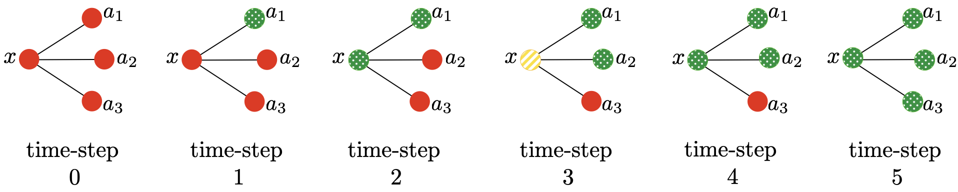
Figure 1: A visualization of the $(1,1)$-protocol for $K_{1,3}$, provided in Example 2.4, with green vertices indicated by dots and the yellow vertex with diagonal lines.

Definition 2.1.

For integers $r\geq 1$ and $s\geq 1$, an $(r,s)$-protocol $J$ for a graph $H$ is a sequence $(A_{1},A_{2},\ldots,A_{N})$ of immunization sets, where $A_{i}\subseteq V(H)$ for $1\leq i\leq N$ and $A_{i}$ is the set of vertices immunized during time-step $i$. The width of $J$, denoted $width(J)$, is the maximum value of $|A_{i}|$ for $1\leq i\leq N$.

Thus, the width of an $(r,s)$-protocol $J$ is the maximum number of immunizations that occur during any given time-step. We sometimes write protocol for $(r,s)$-protocol when the context is clear.

Definition 2.2.

An $(r,s)$-protocol $(A_{1},A_{2},\ldots,A_{N})$ clears graph $H$ if all vertices are green at time-step $N$; that is, $G_{N}=V(H)$.

Every graph $H$ has an $(r,s)$-protocol of width $|V(H)|$ that clears it, namely $A_{1}=V(H)$, and this is the largest width of a protocol for $H$. We next define the $(r,s)$-immunization number of a graph, which is the quantity we seek to minimize.

Definition 2.3.

The $(r,s)$-immunization number of a graph $H$, denoted by $i_{r,s}(H)$, is the smallest width of an $(r,s)$-protocol that clears $H$.

We begin with a simple example that shows $i_{1,1}(K_{1,m})=1$.

Example 2.4.

Let $r=s=1$ and consider $K_{1,m}$, $m\geq 3$, with vertex $x$ of degree $m$ and leaves $a_{1},a_{2},\ldots,a_{m}$. Figure 1 illustrates $K_{1,3}$ and the protocol that we next define. At time-step $0$, all vertices are red. Let $A_{1}=\{a_{1}\}$; that is, vertex $a_{1}$ is immunized during time-step $1$. If nether $a_{1}$ nor $x$ is immunized during time-step $2$, then $a_{1}$ will turn yellow during time-step $2$ (because $r=1$). Let $A_{2}=\{x\}$ and $A_{3}=\{a_{2}\}$. Since $a_{3}$ is not immunized during time-step $3$, $a_{3}$ infects $x$: $x$ becomes yellow during time-step $3$. Inductively, let $A_{2j}=\{x\}$, so $x$ is re-immunized during time-step $2j$, and let $A_{2j+1}=\{a_{j+1}\}$, $2\leq j\leq m-2$. Although $x$ turns yellow on the odd time-steps, it never becomes red and does not reinfect previously immunized vertices. In the last two time-steps, $A_{2m-2}=\{x\}$ and $A_{2m-1}=\{a_{m}\}$. Then, $a_{m}$ does not infect $x$ at time $2m-1$, because it is immunized at that time-step. Thus, the $(1,1)$-protocol $(\{a_{1}\},\{x\},\{a_{2}\},\{x\},\ldots,\{x\},\{a_{m}\})$ clears $K_{1,m}$ because all vertices are green at time-step $2m-1$; that is, $G_{2m-1}=\{x,a_{1},a_{2},a_{3},\ldots,a_{m}\}$.

We next introduce notation that partitions the set of green vertices at time-step $t$ according to the time-step when these vertices were last immunized, and the yellow vertices at time-step $t$ according to when they last became reinfected.

If $v\in A_{t}$,		then $v\in G_{t}^{r}$.
If $v\not\in A_{t}$,	and
	$v\in R_{t-1}$,	then $v\in R_{t}$.
	$v\in Y_{t-1}^{1}$,	then $v\in R_{t}$.
	$v\in Y_{t-1}^{i}$, $2\leq i\leq s$,	then $v\in Y_{t}^{i-1}$.
	$v\in G_{t-1}^{i}$, $2\leq i\leq r$,	then $v\in G_{t}^{i-1}$.
	$v\in G_{t-1}^{1}$ and has a neighbor in $R_{t}$,	then $v\in Y_{t}^{s}$.
	$v\in G_{t-1}^{1}$ and has no neighbor in $R_{t}$,	then $v\in G_{t}^{1}$.

Table 1: Transitions between classes of green, yellow, and red vertices.

Definition 2.5.

Let $H$ be a graph with $(r,s)$-protocol $J=(A_{1},A_{2},\ldots,A_{N})$. We partition the green and yellow vertices at time-step $t$ as follows: $G_{t}=G_{t}^{r}\cup G_{t}^{r-1}\cup\cdots\cup\;G_{t}^{1}$ and $Y_{t}=Y_{t}^{s}\cup Y_{t}^{s-1}\cup\cdots\cup Y_{t}^{1}$ where $G_{t}^{r}=A_{t}$ and the remaining sets are defined by the transitions given in Table 1 and illustrated in Figure 2.

A vertex immunized at time-step $t$ is a member of $G_{t}^{r}$ and if not immunized again, its immunity wanes and it transitions to $G_{t+1}^{r-1}$ and then $G_{t+2}^{r-2}$ and so on, as defined in Table 1. A vertex $v\in G_{t}^{1}$ is susceptible and will become yellow at time-step $t+1$ (i.e., $v\in Y_{t+1}^{s}$) if $v\not\in A_{t+1}$ and $v$ has a neighbor in $R_{t+1}$. A vertex in $Y_{t+1}^{s}$ transitions to $Y_{t+2}^{s-1}$, and so on, eventually to $Y_{t+s}^{1}$ and then $R_{t+s+1}$ unless immunized. Figure 2 illustrates the transitions in Table 1.

Figure 2: A digraph showing the transitions between the states of healthy, infected but not contagious, and contagious.

We record an observation that follows directly from Definition 2.5.

Observation 2.6.

In an $(r,s)$-protocol for a graph $H$, if a vertex is immunized at time $t$ then the earliest it can become red is time-step $t+r+s$.

For the graph $K_{1,3}$, the $(1,1)$-protocol given in Example 2.4 is $\{\{a_{1}\},\{x\},\{a_{2}\},\{x\},\{a_{3}\}\}$. Another $(1,1)$-protocol for $K_{1,3}$ is $J^{\prime}=(\{a_{1}\},\{x\},\{a_{2}\},\{x\},\{a_{3}\},\{a_{1}\})$. Note that it is unnecessary to immunize $a_{1}$ in time-step 6. In a minimal protocol, we do not want to immunize vertices frivolously. We give a formal definition of minimal below.

Definition 2.7.

An $(r,s)$-protocol $(A_{1},A_{2},\ldots,A_{N})$ for graph $H$ is minimal if it satisfies the following for all time-steps $t$ where $1\leq t\leq N$: if $v\in G^{\ell}_{t}$ and $v\in A_{t+1}$ then $v$ has a neighbor in $R_{t+\ell}\cup R_{t+\ell+1}\cup\cdots\cup R_{t+r}$.

We show in Proposition 2.8 that any $(r,s)$-protocol that clears $H$ can be transformed into a minimal protocol.

Proposition 2.8.

Let $J$ be an $(r,s)$-protocol $(A_{1},A_{2},\ldots,A_{N})$ that clears $H$. Then there exists a minimal protocol $J^{\prime}=(A^{\prime}_{1},A^{\prime}_{2},\ldots,A^{\prime}_{N})$ that clears $H$ and for which $A^{\prime}_{i}\subseteq A_{i}$, $1\leq i\leq N$.

Proof.

Let $v\in A_{N}$. Since $J$ clears $H$, all vertices are in $G_{N}$. Thus, any vertices that are not green at time-step $N-1$ must be in $A_{N}$. Any vertex that is green at time-step $N-1$ remains green at time-step $N$ without needing to be immunized, because any red neighbor will be in $A_{N}$. Hence we can replace $A_{N}$ by $A^{\prime}_{N}=A_{N}-(G_{N-1}\cap A_{N})$. By induction, assume that we have a protocol $(A_{1},A_{2},\ldots,A_{k+1},A^{\prime}_{k+2},A^{\prime}_{k+3},\ldots,A^{\prime}_{N})$ such that for all time-steps $t$ where $k+1\leq t\leq N-1$: if $v\in G^{\ell}_{t}$ and $v\in A^{\prime}_{t+1}$ then $v$ has a neighbor in $R_{t+\ell}\cup R_{t+\ell+1}\cup\cdots\cup R_{t+r}$. Consider any vertex $v\in G^{\ell}_{k}\cap A_{k+1}$ that does not have a neighbor in $R_{k+\ell}\cup R_{k+\ell+1}\cup\cdots\cup R_{k+r}$. Because the protection $v$ gets from being immunized at time-step $k+1$ only lasts until time-step $k+r$, if $v$ has no red neighbors in that time period, then the immunization is unnecessary. Let $W$ be the set of such vertices $v$. Then we can replace $A_{k+1}$ by $A^{\prime}_{k+1}=A_{k+1}-W$, and the protocol $(A_{1},A_{2},\ldots,A_{k},A^{\prime}_{k+1},A^{\prime}_{k+2},A^{\prime}_{k+3},\ldots,A^{\prime}_{N})$ clears $H$. Hence our final protocol $(A^{\prime}_{1},A^{\prime}_{2},\ldots,A^{\prime}_{N})$ clears $H$ and is minimal. ∎

2.2 Immunizations of subgraphs

Figure 3 shows a graph $H$ with $i_{1,1}(H)=1$ and a subgraph $H^{\prime}$ of $H$. In this figure, $(1,1)$-protocols are shown for $H$ and $H^{\prime}$ by labeling each vertex by the set of time-steps at which it is immunized, unlike in Figure 1. Observe that the protocol $J^{\prime}$ shown for $H^{\prime}$ is inherited from the protocol $J$ for $H$ by restricting each immunization set to vertices in $H^{\prime}$. The next theorem shows how to generalize this example.

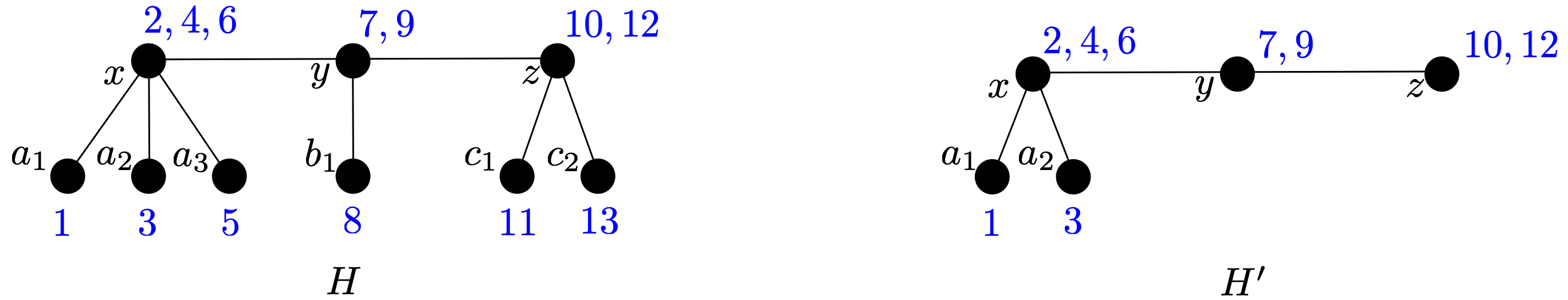
Figure 3: A protocol $J$ that clears $H$ and the restricted protocol $J^{\prime}$ that clears subgraph $H^{\prime}$. A vertex has label $t$ if it is immunized at time-step $t$.

Theorem 2.9.

Let $H$ be a graph and $(A_{1},A_{2},\dots,A_{N})$ be an $(r,s)$-protocol that clears $H$. If $H^{\prime}$ is a subgraph of $H$, and $A^{\prime}_{i}=A_{i}\cap V(H^{\prime})$, for $1\leq i\leq N$, then graph $H^{\prime}$ is cleared by $(r,s)$-protocol $(A_{1}^{\prime},A_{2}^{\prime},\dots,A_{N}^{\prime})$.

Proof.

Let $J=(A_{1},A_{2},\dots,A_{N})$ and $J^{\prime}=(A_{1}^{\prime},A_{2}^{\prime},\dots,A_{N}^{\prime})$. Since $J$ clears $H$, all vertices of $H$ are green at the end of time-step $N$ under protocol $J$. For a contradiction, suppose that $J^{\prime}$ does not clear $H^{\prime}$; hence there is some vertex in $V(H^{\prime})$ that is not green at the end of time-step $N$ under protocol $J^{\prime}$. Let $t$ be the smallest integer such that there exists $w\in V(H^{\prime})$ that is green at time-step $t$ under $J$, but not green under $J^{\prime}$; that is, $w\in G_{t}(H)$, but $w\not\in G_{t}(H^{\prime})$. By the minimality of our choice of $t$, we know $w\in G_{t-1}(H)\cap G_{t-1}(H^{\prime})$. Since $w\not\in G_{t}(H^{\prime})$, $w$ has a neighbor $x$ in $H^{\prime}$ such that $x\in R_{t}(H^{\prime})$ and $x\not\in R_{t}(H)$. Since $x\not\in R_{t}(H)$, vertex $x$ must have been immunized at some time-step before $t$. Consider the last time-step $j$ for which $x$ was immunized, in both protocols, before time-step $t$. Then because $x$ is red at time $t$ under $J^{\prime}$, then $x$ must be infected between time-steps $j$ and $t$. By the minimality of $t$ and the choice of $w$, $x$ must turn yellow at the same time under both $J$ and $J^{\prime}$. Since $x$ is not immunized between time-steps $j$ and $t$, vertex $x$ turns red at the same time in both protocols, contradicting $x\in R_{t}(H^{\prime})$ and $x\not\in R_{t}(H)$. ∎

An immediate consequence of Theorem 2.9 is that the $(r,s)$-immunization number of a graph is at least as large as the $(r,s)$-immunization number of each of its subgraphs.

Corollary 2.10.

If $H^{\prime}$ is a subgraph of $H$, then $i_{r,s}(H^{\prime})\leq i_{r,s}(H)$.

3 Immunization number and pathwidth

In this section, we use the notion of path decompositions to bound our parameter from above, and then go on to make use of two particular types of protocols that we will call monotone and cautious.

3.1 An upper bound for the immunization number using pathwidth

As the example in Figure 3 demonstrates, if a graph has a path-like ordering of vertices, this ordering can be used to construct a protocol. The next definition of path decomposition formalizes this notion and Theorem 3.4 uses the resulting pathwidth to provide an upper bound for the $(r,s)$-immunization number.

Definition 3.1.

A path decomposition of a graph $H$ is a sequence $(B_{1},\dots,B_{m})$ where each $B_{i}$ is a subset of $V(H)$ such that (i) if $xy\in E(H)$ then there exists an $i$, for which $x,y\in B_{i}$ and (ii) for all $w\in V(H)$, the set of $B_{i}$ containing $w$ forms a consecutive subsequence; that is, if $w\in B_{i}$ and $w\in B_{k}$ and $i\leq j\leq k$ then $w\in B_{j}$.

The subsets $B_{1},\dots,B_{m}$ are often referred to as bags of vertices. We can think of the sequence $(B_{1},\dots,B_{m})$ as forming the vertices of a path $P$. Conditions (i) and (ii) ensure that if two vertices are adjacent in $H$, they are in some bag together and that the bags containing any particular vertex of $H$ induce a subpath of $P$. The graph $K_{1,3}$, shown in Figure 1, has a path decomposition with bags $B_{1}=\{a_{1},x\}$, $B_{2}=\{a_{2},x\}$, $B_{3}=\{a_{3},x\}$. The width of a path decomposition and the pathwidth of a graph are defined below in such a way that the pathwidth of a path is 1.

Definition 3.2.

The width of a path decomposition $(B_{1},\dots,B_{m})$ is $\max_{1\leq i\leq m}|B_{i}|-1$ and the pathwidth of a graph $H$, denoted $pw(H)$, is the minimum width taken over all path decompositions of $H$.

The next example illustrates the proof technique for Theorem 3.4.

Example 3.3.

We provide a $(1,2)$-protocol for the Cartesian product $P_{4}\square P_{4}$ based on a minimum width path decomposition. It is well known that $pw(P_{4}\square P_{4})=4$; for example, see [4]. Since our protocol will have width 2 and $\lceil(1+4)/(1+2)\rceil=2$, our protocol will achieve the upper bound in Theorem 3.4.

Figure 4 illustrates the bags in such a path decomposition and each bag is divided into $3$ sections, where the sections of bag $B_{i}$ are: section 1, section 2, section 3. Observe that each vertex that appears in multiple bags always occurs in the same section of those bags.

Starting at bag $B_{1}$, create a $(1,2)$-protocol where, in a given bag $B_{i}$, we immunize vertices in section 1, 2, 3, then section 1, 2, 3 again; after this, we move to bag $B_{i+1}$ and repeat the process. Thus, in our example $A_{1}=A_{4}=\{v_{1},v_{2}\}$, $A_{2}=A_{5}=\{v_{3},v_{4}\}$, $A_{3}=A_{6}=\{v_{5}\}$, $A_{7}=A_{10}=\{v_{2},v_{6}\}$, $A_{8}=A_{11}=\{v_{3},v_{4}\}$, $A_{9}=A_{12}=\{v_{5}\}$, and so on. One can verify this leads to a $(1,2)$-protocol that clears $P_{4}\square P_{4}$. In particular, observe that for each vertex $v$, if we consider the time period between the first and last time-step $v$ is immunized, it is immunized exactly every $r+s$ time-steps. By Observation 2.6, vertex $v$ does not turn red during this time period and indeed in this protocol, once a vertex is green, it never again becomes red.

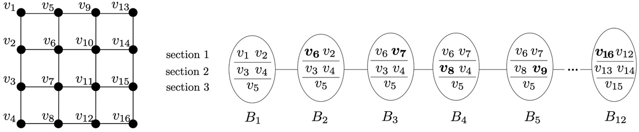
Figure 4: A minimum width path decomposition of $P_{4}\square P_{4}$. The bold vertices are replacements as we move from left to right in the path.

Theorem 3.4.

If $H$ is a graph then $i_{r,s}(H)\leq\lceil\frac{1+pw(H)}{r+s}\rceil.$

Proof.

Let $(B_{1},\dots,B_{m})$ be a path decomposition of $H$ whose width is $pw(H)$. By Definition 3.2 we know that $|B_{i}|\leq 1+pw(H)$ for $1\leq i\leq m$. For each $k$, we will partition $B_{k}$ into $r+s$ sections, $sct(k,1),sct(k,2),\ldots,sct(k,r+s)$, some of which may be empty. We use these sections to create an $(r,s)$-protocol $(A_{1},\dots,A_{N})$ for graph $H$. In this protocol, we will immunize vertices one bag at a time. For each bag, we twice cycle through its sections, as in Example 3.3. Each partition of $B_{k}$ into $r+s$ sections will lead to $2(r+s)$ time-steps in the protocol.

Partition the vertices of $B_{1}$ arbitrarily into $sct(1,1),sct(1,2),\ldots,sct(1,r+s)$. Let $A_{j}=A_{(r+s)+j}=sct(1,j)$ for $1\leq j\leq r+s$. By construction, at the end of time-step $r+s$, all vertices in $B_{1}$ are green or yellow. At the end of time-step $2(r+s)$, we have the additional property that any vertex in $B_{1}$, all of whose neighbors are also in $B_{1}$, is green. Thus, at the end of time-step $2(r+s)$, any yellow vertex in $B_{1}$ has a red neighbor in $B_{2}$.

Partition $B_{2}$ into $r+s$ sets $sct(2,1),sct(2,2),\dots,sct(2,r+s)$ where $B_{2}\cap sct(1,i)\subseteq sct(2,i)$ for $1\leq i\leq r+s$, that is, vertices of $B_{2}$ that are in section $i$ of $B_{1}$ are placed in section $i$ of $B_{2}$. Distribute the vertices in $B_{2}-B_{1}$ arbitrarily into $sct(2,1),sct(2,2),\dots,sct(2,r+s)$ so that each set has at most $\lceil\frac{1+pw(H)}{r+s}\rceil$ vertices. Let $A_{2(r+s)+1}=sct(2,1)$, $A_{2(r+s)+2}=sct(2,2)$, $\dots$, $A_{3(r+s)}=sct(2,r+s)$ (the first cycle of immunizations for $B_{2}$) and $A_{3(r+s)+i}=A_{2(r+s)+i}$ for $1\leq i\leq r+s$ (the second cycle of immunizations for $B_{2}$).

At the end of time-step $4(r+s)$ all vertices in $B_{1}\cup B_{2}$ are green or yellow and any yellow vertices have a red neighbor in $B_{3}$.

We continue by induction. Suppose we have considered $B_{1},\dots,B_{k}$ and extended our protocol so that at the end of time-step $2k(r+s)$ all vertices in $B_{1}\cup\dots\cup B_{k}$ are green or yellow and any yellow vertices have a red neighbor in $B_{k+1}$. We now partition $B_{k+1}$ into $r+s$ sets $sct(k+1,1),sct(k+1,2),\dots,sct(k+1,r+s)$ so that $B_{k+1}\cap sct(k,i)\subseteq sct(k+1,i)$ for $1\leq i\leq r+s$. Distribute the vertices in $B_{k+1}-B_{k}$ arbitrarily into $sct(k+1,1),sct(k+1,2),\dots,sct(k+1,r+s)$ so that each set again has at most $\lceil\frac{1+pw(H)}{r+s}\rceil$ vertices. Let $A_{2k(r+s)+1}=sct(k+1,1)$, $A_{2k(r+s)+2}=sct(k+1,2)$, $\dots$, $A_{2k(r+s)}=sct(k+1,r+s)$; and $A_{(2k+1)(r+s)+i}=A_{(2k)(r+s)+i}$ for $1\leq i\leq r+s$.

At the end of time-step $(2k+2)(r+s)$ all vertices in $B_{1}\cup\dots\cup B_{k+1}$ are green or yellow and any yellow vertices have a red neighbor in $B_{k+2}$, provided $B_{k+2}$ exists. Since $B_{m}$ is the highest-indexed bag, at time-step $2m(r+s)$, all vertices in $B_{1}\cup\dots\cup B_{m}$ are green. Therefore, our protocol $(A_{1},\dots,A_{N})$ clears graph $H$ with $N=2m(r+s)$ and furthermore, the $|A_{i}|\leq\lceil(1+pw(H))/(r+s)\rceil$.∎

3.2 Nested sets of infected vertices

In this section we consider two special types of protocols: monotone (Definition 3.5) and cautious (Definition 3.7). In a monotone protocol, once a vertex is immunized it never again becomes contagious. Thus, over time, the sets of contagious vertices are nested; at each time-step the current set of contagious vertices is a subset of those at the previous time-step. Inspired by Observation 2.6, we define an $(r,s)$-protocol to be cautious if for each vertex $v$, in between the first and last time-steps in which $v$ is immunized, it is immunized at least every $r+s$ time-steps.

Definition 3.5.

An $(r,s)$-protocol $(A_{1},A_{2},\ldots,A_{N})$ that clears graph $H$ is monotone if it satisfies the following: for all $v\in V(H)$, if $v\in A_{j}$ then $v\not\in R_{i}$ for all $i>j$.

Bernshteyn and Lee [1] define a protocol to be monotone if green vertices never become red again; however, in their model, there are no yellow vertices. Our model combines yellow and green vertices in the definition of monotone.

The next proposition shows that we can equivalently define a protocol to be monotone if vertices that are about to be contagious are immunized.

Proposition 3.6.

Let $J$ be an $(r,s)$-protocol for graph $H$ where $J=(A_{1},A_{2},\ldots,A_{N})$. Then $J$ is monotone if and only if for every $j:1\leq j\leq N$ and every $v\in Y_{j}^{1}$, we have $v\in A_{j+1}$.

Proof.

First suppose that $J$ is a monotone $(r,s)$-protocol for graph $H$. Since all vertices are initially red, if $v\in Y_{j}^{1}$ then $v\in A_{i}$ for some $i:1\leq i<j$. If in addition $v\not\in A_{j+1}$, then $v\in R_{j+1}$, contradicting the definition of monotone.

Conversely, in protocol $J$, if every vertex in $Y_{j}^{1}$ is also in $A_{j+1}$ then, once a vertex is immunized, it never becomes red. Hence, $J$ is monotone.∎

In Observation 2.6 we noted that a vertex that is immunized at time-step $j$ cannot become contagious until $r+s$ time-steps later. Thus we can achieve a monotone protocol by immunizing vertices frequently. We define what it means for a protocol to be cautious in Definition 3.7 and in Theorem 3.8 prove that cautious protocols are monotone. Note that the protocols for graphs $H$ and $H^{\prime}$ in Figure 3 are cautious and monotone.

Definition 3.7.

Let $H$ be a graph and suppose that $(A_{1},A_{2},\ldots,A_{N})$ is an $(r,s)$-protocol that clears $H$. We say that this $(r,s)$-protocol is cautious if the following holds for all vertices $w\in V(H)$: if the first occurrence of $w$ in an immunization set is in $A_{j}$ and the last is in $A_{k}$, then among any $r+s$ consecutive elements of the sequence $A_{j},A_{j+1},\dots,A_{k}$, at least one must contain $w$.

Theorem 3.8.

Any cautious $(r,s)$-protocol for graph $H$ is monotone.

Proof.

Let $J$ be a cautious $(r,s)$-protocol for graph $H$ with $J=(A_{1},A_{2},\ldots,A_{N})$. By the definition of cautious we know $J$ clears $H$ and we will show that $J$ is monotone. Consider $v\in V(H)$ and let the first occurrence of $v$ be in $A_{j}$ and the last in $A_{k}$. By Observation 2.6, we know that $v$ is not red between time-steps $j$ and $k$ because $J$ is cautious. Since $J$ clears $H$, we also know that $v$ is green at time-step $N$. If $v$ were red after time-step $k$ then it would need to be immunized after time-step $k$ in order to be green at time-step $N$, contradicting our choice of $k$. Thus $J$ is monotone. ∎

Not all monotone protocols are cautious. For example, the $(1,1)$-protocol $(\{a_{1}\},\{x\},\{a_{2}\},\{x\},\{a_{3}\},\{a_{1}\})$ for the graph $K_{1,3}$ as labeled in Figure 1 is monotone but not cautious, because $a_{1}$ is immunized at the first time-step and then again 5 time-steps later; however $r+s=2$. As previously discussed, $J^{\prime}$ is not minimal; that is, it is unnecessary to immunize vertex $a_{1}$ in time-step 6. In Theorem 3.9 we show that protocols that are both monotone and minimal are always cautious.

Theorem 3.9.

If $J$ is a minimal and monotone $(r,s)$-protocol for graph $H$, then $J$ is cautious.

Proof.

For a proof by contradiction, suppose $J$ is not cautious. Then $\exists w\in V(H)$ with first occurrence in $A_{j}$ and last in $A_{k}$ such that $w\not\in A_{t}\cup A_{t+1}\cup\cdots\cup A_{t+r+s-1}$ and $w\in A_{t+r+s}$, with $j<t$ and $t+r+s-1<k$. Because $J$ is monotone, $w$ is never red after time-step $j$, and therefore it is green or yellow at time-step $t+r+s-1$. Now $w$ was last immunized at or before time-step $t-1$, so if $w$ is green at time $t+r+s-1$, then $w\in G^{1}_{t+r+s-1}$. Otherwise, $w\in Y_{t+r+s-1}$. We consider these cases separately.

If $w\in G^{1}_{t+r+s-1}$, since $w\in A_{t+r+s}$, then by definition of minimality, $w$ has a neighbor $y\in R_{t+r+s}\cup R_{t+r+s+1}\cup\cdots R_{t+r+s+r-1}$. By monotonicity, vertex $y$ has been red from time-step 1 at least until time-step $t+r+s$. In particular, $y$ is red in the time-steps $t,t+1,t+2,\ldots,t+r+s-1$. Vertex $w$ was last immunized at or before time-step $t-1$, so by time-step $t+r-1$, it has no immunity remaining, and it is infected by its neighbor $y$. Thus, vertex $w$ turns red $s$ time-steps later, and is red at time-step $t+r+s-1$, because it is not immunized in that time period. This contradicts $w\in G^{1}_{t+r+s-1}$.

Otherwise, $w\in Y_{t+r+s-1}$. In this case, $w$ was infected at most $s$ time-steps previously, so it was infected at time $t+r$ or later, because it remains yellow for at most $s$ time-steps. Vertex $w$ was last immunized at or before time-step $t-1$, and its immunity lasted until time-step $t+r-2$ or sooner. Thus, vertex $w$ is infected by its neighbor $y$ at time-step $t+r-1$, and thus became red $s$ time-steps later, and is red at time-step $t+r+s-1$. This contradicts $w\in Y_{t+r+s-1}$.∎

In Theorem 3.10, we show that using a cautious protocol $J$ to clear $H$ yields a path decomposition of $H$, and that $width(J)\geq\lceil(\mbox{$1+$ pathwidth of $H$})/2\rceil$. Together with Theorem 3.9, we get the same upper bound for monotone protocols that are minimal.

Theorem 3.10.

If $J$ is a cautious $(r,s)$-protocol that clears graph $H$, then $width(J)\geq\lceil\frac{1+pw(H)}{r+s}\rceil$.

Proof.

Let $J=(A_{1},A_{2},\dots,A_{N})$ and let $m=N-(r+s)+1$. We will create a path decomposition of $H$ with bags $B_{1},B_{2},\dots,B_{m}$ where each $B_{i}$ is the union of $r+s$ immunization sets, and thus $|B_{i}|\leq(r+s)\cdot width(J)$ for $1\leq i\leq m$. Thus,

$$width(J)\geq\frac{\max_{1\leq i\leq m}|B_{i}|}{r+s}\geq\frac{1+pw(H)}{r+s}.$$

Since the width of $J$ is an integer, it suffices to construct the path decomposition. The path decomposition construction in this proof is illustrated below in Example 3.11.

Define the bags $B_{i}$ as $B_{i}=A_{i}\cup A_{i+1}\cup\dots\cup A_{i+(r+s-1)}$ for $1\leq i\leq m$. Note that $A_{i}$ first appears in $B_{i-(r+s-1)}$ and last appears in $B_{i}$ (or $B_{1}$ if $i-(r+s-1)<0$). It remains to show the bags $B_{1},\dots,B_{m}$ form a path decomposition.

To prove (ii) of Definition 3.1, let $w$ be a vertex in $H$ and let $A_{j}$ be the first element of $J$ that contains $w$, and $A_{k}$ be the last element of $J$ that contains $w$. As noted above, this means $w\in B_{j-(r+s-1)}$ and $w\in B_{k}$. Because $J$ is cautious, there is no sequence of $r+s$ consecutive time-steps between $j$ and $k$ in which $w$ is not immunized; so $w$ is in every bag from $B_{j-(r+s-1)}$ to $B_{k}$ (again, or from $B_{1}$ if $j-(r+s-1)<0$).

Now to prove (i) of Definition 3.1, suppose for a contradiction that $uw$ is an edge in $H$ and no bag contains $uw$. Without loss of generality, suppose that the first occurrence of $u$ is earlier than the first occurrence of $w$ in $J$. Let the first occurrence of $u$ be in $A_{j}$ and the last in $A_{k}$. Then $u$ is in bags $B_{j-(r+s-1)},B_{j-(r+s-2)},\dots,B_{k}$ and note that $B_{k}=A_{k}\cup A_{k+1}\cup\dots\cup A_{k+(r+s-1)}$. The lowest-indexed bag that could contain $w$ is $B_{k+1}$, and thus the lowest-indexed immunization set that can contain $w$ is $A_{k+(r+s)}$. Since $u$ was last immunized during time-step $k$, at time-step $k+(r+s-1)$, it would have been infected by $w$, contradicting the fact that the immunization protocol clears $H$. ∎

Example 3.11.

To illustrate the construction given in the proof of Theorem 3.10, we start with the graph $H$ and a $(1,1)$-protocol that clears it, both of which are shown in Figure 3. The construction results in the path decomposition of $H$ that has the following $12$ bags: $B_{1}=\{a_{1},x\}$, $B_{2}=\{x,a_{2}\}$, $B_{3}=\{a_{2},x\}$, $B_{4}=\{x,a_{3}\}$, $B_{5}=\{a_{3},x\}$, $B_{6}=\{x,y\}$, $B_{7}=\{y,b_{1}\}$, $B_{8}=\{b_{1},y\}$, $B_{9}=\{y,z\}$, $B_{10}=\{z,c_{1}\}$, $B_{11}=\{c_{1},z\}$, $B_{12}=\{z,c_{2}\}$.

We conclude this section with a corollary for graphs $H$ for which there is strict inequality in Theorem 3.4.

Corollary 3.12.

Let $H$ be a graph such that $i_{r,s}(H)<\left\lceil\frac{1+pw(H)}{r+s}\right\rceil$. The only $(r,s)$-protocols that clear $H$ and have width $i_{r,s}(H)$ are non-cautious $(r,s)$-protocols.

Proof.

By Theorem 3.10, every cautious $(r,s)$-protocol for $H$ will have width at least $i_{r,s}(H)$. Thus, the only way to find an $(r,s)$-protocol that achieves $i_{r,s}(H)<\left\lceil\frac{1+pw(H)}{r+s}\right\rceil$ is to use a non-cautious $(r,s)$-protocol. ∎

4 The immunization number when $r=s=1$

In the next sections, we provide results for the case where $r=s=1$. For a graph $H$, we let $i_{1,1}(H)=i(H)$ for the rest of the paper and abbreviate $(1,1)$-protocol by protocol and abbreviate $(r,s)$-immunization number by immunization number. For a subset $S\subseteq V(H)$, we define the neighborhood of $S$ to be $N(S)=\{v\in N(x)|x\in S\}$ and note that some vertices of $S$ may be in $N(S)$.

4.1 Characterization of graphs with immunization number 1

If a protocol of width 1 clears a graph, then the number of green vertices can be increased from one time-step to the next only when there is at most one infected (yellow or red) vertex that is adjacent to a green vertex. This leads to the following necessary condition for graphs $H$ with $i(H)=1$.

Lemma 4.1.

If $H$ is a graph with $i(H)=1$ then, for every $p$ with $1\leq p\leq|V(H)|-1$, there exists $S\subseteq V(H)$ with $|S|=p$ and $|N(S)-S|\leq 1$.

Proof.

Let $H$ be a graph with $i(H)=1$ and let $(A_{1},A_{2},\ldots,A_{N})$ be a protocol that clears $H$ with $|A_{i}|\leq 1$ for each $i$. The only way for a vertex to become green is to be immunized, so the number of green vertices increases by at most $1$ at each time-step. This protocol clears $H$, so for $p$ with $1\leq p\leq|V(G)|-1$ there is a time-step $j$ in which the number of green vertices increases from $p$ to $p+1$. The set $G_{j}$ consists of the $p$ green vertices at time-step $j$, and they must remain green at time-step $j+1$ while a new vertex is immunized. If there were two vertices in the set $N(G_{j})-G_{j}$ then at most one of these could be immunized at time-step $j+1$ and the other would reinfect a vertex of $G_{j}$, a contradiction. Thus $|N(G_{j})-G_{j}|\leq 1$ and the set $G_{j}$ is our desired set $S$.∎

Let $K^{\prime}_{1,3}$ be the graph obtained by subdividing each edge of $K_{1,3}$ exactly once and let $C_{n}$ be a cycle on $n\geq 3$ vertices. We next use Lemma 4.1 to determine the immunization number of $C_{n}$ and $K_{1,3}^{\prime}$ and then use these results to characterize graphs with immunization number $1$. Every vertex of a cycle has two neighbors, so the conclusion of Lemma 4.1 fails when $p=1$. Thus $i(C_{n})\geq 2$. The following protocol shows that $i(C_{n})\leq 2$. First immunize two adjacent vertices, and at each subsequent time-step, immunize the infected neighbors of the vertices most recently immunized. An alternate proof is to use Theorem 3.4 and that fact that the pathwidth of $C_{n}$ is $2$; see [4]. We record this in Observation 4.2.

In $K^{\prime}_{1,3}$, every set $S$ of $3$ vertices has $|N(S)-S|\geq 2$. Therefore, $i(K^{\prime}_{1,3})\geq 2$ by Lemma 4.1. It is an easy exercise to find a protocol of width $2$ that clears $K^{\prime}_{1,3}$. Thus $i(K^{\prime}_{1,3})=2$, which we also record in Observation 4.2.

Observation 4.2.

The immunization number of any cycle is $2$ and the immunization number of $K^{\prime}_{1,3}$ is $2$.

We now characterize those graphs $H$ for which $i(H)=1$. A caterpillar is a graph that consists of a path together with zero or more leaves incident to each vertex of the path.

Theorem 4.3.

For a graph $H$ that contains at least one edge, $i(H)=1$ if and only if $H$ is a caterpillar.

Proof.

Let $H$ be a caterpillar. Note that the pathwidth of a caterpillar is one; see [4]. Now Theorem 3.4 (with $r=s=1$) implies that $i(H)\leq 1$. Since $H$ contains at least one edge, $i(H)\geq 1$. Thus, $i(H)=1$.

For the other direction, we assume $H$ is a graph that contains at least one edge and $i(H)=1$. It is well known that caterpillars are precisely those trees that have no induced $K^{\prime}_{1,3}$. By Observation 4.2, cycles have immunization number $2$, so by Corollary 2.10, $H$ cannot contain a cycle as a subgraph and hence $H$ is a tree. Similarly, by Observation 4.2, the graph $K^{\prime}_{1,3}$ has immunization number 2, and so it cannot be a subgraph of $H$, and hence $H$ is a caterpillar. ∎

4.2 A tool for finding lower bounds of $i(H)$

We generalize Lemma 4.1 that helped characterize graphs with immunization number 1. For any protocol that clears graph $H$, the number of green vertices must increase beyond each threshold from 2 to $|V(H)|-1$. Every time there is an increase, some set $S$ of vertices will remain green without being immunized. The number of infected neighbors of vertices in $S$ is restricted based on the number of immunizers available.

Theorem 4.4.

Let $H$ be a graph. For each $p:i(H)+1\leq p\leq|V(H)|-1$ there exists a set $S\subseteq V(H)$ with $p-i(H)+1\leq|S|\leq p$ so that $|N(S)-S|\leq 2\,i(H)-1$.

Proof.

Let $(A_{1},A_{2},\ldots,A_{N})$ be a protocol that clears graph $H$ with $|A_{i}|\leq i(H)$ for each $i$. Thus $G_{N}=V(H)$; that is, all vertices are green at time-step $N$. For any $p$ with $i(H)+1\leq p\leq|V(H)|-1$, there must be a time-step $j$ for which $|G_{j}|\leq p$ and $|G_{j+1}|\geq p+1$. The only way for a vertex to become green is to be immunized, so the number of green vertices increases by at most $i(H)$ at each time-step and hence $|G_{j}|\geq|G_{j+1}|-i(H)\geq p+1-i(H)$.

We partition $G_{j}$ into three parts: $G_{j}\cap Y_{j+1}$ (vertices in $G_{j}$ that are infected at time-step $j+1$), $G_{j}\cap A_{j+1}$ (vertices in $G_{j}$ that are immunized at time-step $j+1$), and the set $S$ of remaining vertices (vertices of $G_{j}$ that remain green at time-step $j+1$ without being re-immunized). In addition, let $a=|G_{j}\cap Y_{j+1}|$, let $b=|G_{j}\cap A_{j+1}|$, and let $k=|A_{j+1}\cap\overline{G_{j}}|$, the number of vertices outside of $G_{j}$ that are immunized at time-step $j+1$.

First we show the condition $p-i(H)+1\leq|S|\leq p$. The upper bound follows immediately from $|S|\leq|G_{j}|\leq p$. For the lower bound, since $|G_{j}|\geq p+1-i(H)$, we can write $|G_{j}|=p-d$ for some integer $d$ with $0\leq d\leq i(H)-1$. Since there are $k$ vertices outside of $G_{j}$ immunized at time-step $j+1$ and $a$ vertices of $G_{j}$ that become infected at time-step $j+1$, we have $|G_{j+1}|=|G_{j}|+k-a$. Recall that $|G_{j+1}|\geq p+1$, and hence $k-a=|G_{j+1}|-|G_{j}|\geq(p+1)-(p-d)=d+1$. We conclude that $d+a\leq k-1$ or equivalently $-d-a\geq-k+1$. Also note that there are exactly $b+k$ vertices immunized at time-step $j+1$, so $b+k\leq i(H)$, or equivalently, $-b-k\geq-i(H)$. Now we complete the proof of the lower bound on $|S|$ as follows:

$$|S|=|G_{j}|-b-a=p-d-b-a=p-b+(-d-a)\geq p-b+(-k+1)=p+1+(-b-k)\geq p+1-i(H).$$

It remains to show the inequality $|N(S)-S|\leq 2\,i(H)-1$. By construction, $|G_{j}|=|S|+a+b$. By definition, the vertices of $S$ remain healthy at time-step $j+1$ so their only neighbors can be other vertices in $G_{j}$ and the $k$ vertices outside of $G_{j}$ that are immunized at time-step $j+1$, because all other vertices are contagious. Thus $|N(S)-S|\leq a+b+k$. However, $k+b=|A_{j+1}|\leq i(H)$. Combining these we obtain the following: $|N(S)-S|\leq a+b+k\leq a+i(H).$

Recall that $|G_{j+1}|\geq p+1\geq|G_{j}|+1$; that is, there are more healthy vertices at time-step $j+1$ than at time-step $j$. There are $a$ newly infected vertices, so there must be more than $a$ newly immunized vertices, and thus $|A_{j+1}|\geq a+1$. Therefore, $i(H)\geq|A_{j+1}|\geq a+1$ and we obtain $|N(S)-S|\leq a+i(H)\leq(i(H)-1)+i(H)=2i(H)-1$, as desired. ∎

As a special case, if $H$ is a graph with $i(H)=2$ then for every $p$ with $2\leq p\leq|V(H)|-1$ there exists $S\subseteq V(H)$ with $|S|=p-1$ or $p$ and $|N(S)-S|\leq 3$. The next two results use this special case of Theorem 4.4.

Proposition 4.5.

The Petersen graph has immunization number $3$.

Proof.

Let $H$ be the Petersen graph. It is well known that $H$ can be represented so that $V(H)$ is the set of $2$-element subsets of $\{1,2,3,4,5\}$ and two vertices are adjacent precisely when their corresponding subsets are disjoint. One can check that the following immunization protocol clears $H$: $A_{1}=\{12,34,35\}$,  $A_{2}=\{15,25,45\}$,  $A_{3}=\{13,23,35\}$,  $A_{4}=\{14,24,25\}$,  $A_{5}=\{15,23,34\}$. Thus $i(H)\leq 3$.

It remains to show $i(H)>2$. We know that $i(H)\neq 1$ by Theorem 4.3. Suppose for a contradiction that $i(H)=2$. By Theorem 4.4, we know that for each $p:3\leq p\leq 9$, there exists $S\subseteq V(H)$ with $p-1\leq|S|\leq p$ so that $|N(S)-S|\leq 3$. Consider $p=3$. For all $S\subseteq V(H)$ with $|S|=p-1=2$ one can check that $|N(S)-S|\geq 4>3$. Likewise, for all $S\subseteq V(H)$ with $|S|=p=3$ one can check that $|N(S)-S|\geq 5>3$. This is a contradiction.∎

For a set $S$, the set $N(S)-S$ represents the boundary of $S$; that is, the expression represents the neighbors of $S$ that are not in $S$. This quantity has also been studied in the context of the vertex isoperimetric value of a graph; see the surveys [3, 15]. We combine Theorem 4.4 with the known isoperimetric value of the grid to find the immunization number of the grid.

Definition 4.6.

Let $H$ be a graph. For $k\in\{1,2,\dots,|V(H)|\}$, the vertex isoperimetric value of graph $H$ with integer $k$ is denoted $\Phi_{V}(H,k)$, and is defined as

$$\Phi_{V}(H,k)=\min_{S\subseteq V(H):|S|=k}|N(S)-S|.$$

Consider, for example, $P_{4}\square P_{4}$, as shown in Figure 4. The interested reader can verify that for any set $S$ of eight vertices, there are at least four vertices not in $S$ that have a neighbor in $S$; that is, $|N(S)-S|\geq 4$. Since we can find a set of eight vertices which have exactly four neighbors not in the set, $\Phi_{V}(P_{4}\square P_{4},8)=4$.

Theorem 4.7.

For $n\geq 3$, $i(P_{n}\square P_{n})=\lceil\frac{n+1}{2}\rceil$.

Proof.

Assume $n\geq 3$. It is well known that $pw(P_{n}\square P_{n})=n$ (see [4]). By Theorem 3.4, $i(P_{n}\square P_{n})\leq\lceil\frac{n+1}{2}\rceil$. Thus, $i(P_{n}\square P_{n})=\lceil\frac{n+1}{2}\rceil-\ell$ for some integer $\ell\in\{0,1,\dots,\lceil\frac{n-1}{2}\rceil\}$.

Let $p=\frac{n^{2}+n-2}{2}$ and observe that $\lceil\frac{n+1}{2}\rceil-\ell+1\leq p\leq n^{2}-1$ because $n\geq 3$. Thus, by Theorem 4.4, there exists a set $S\subseteq V(P_{n}\square P_{n})$ with

$$p-\left(\left\lceil\frac{n+1}{2}\right\rceil-\ell\right)+1\leq\;|S|\;\leq p$$

so that $|N(S)-S|\leq 2(\lceil\frac{n+1}{2}\rceil-\ell)-1$. We simplify the latter inequality:

$$|N(S)-S|\leq 2\Big{\lceil}\frac{n+1}{2}\Big{\rceil}-2\ell-1=\begin{cases}n-2\ell&\text{ if $n$ is odd,}\\ n+1-2\ell&\text{ if $n$ is even.}\end{cases}$$ (1)

To complete the proof, we use the following result, proven in [5] and explicitly stated in [6]:

$$\Phi_{V}(P_{n}\square P_{n},k)=n\text{~{}~{}for~{}~{}}\frac{n^{2}-3n+4}{2}\leq k\leq\frac{n^{2}+n-2}{2}.$$

Consequently,

$$|N(S)-S|\geq n\text{~{}~{}for~{}~{}}\frac{n^{2}-3n+4}{2}\leq|S|\leq\frac{n^{2}+n-2}{2}.$$

But this contradicts the inequality in (1) unless $\ell=0$. Thus, for $n\geq 3$, $i(P_{n}\square P_{n})=\lceil\frac{n+1}{2}\rceil$. ∎

5 Subdivisions when $r=s=1$

The main result of this section is proving that every tree has a subdivision that has immunization number at most 2. We begin with $P_{4}\square P_{4}$, to illustrate how subdividing an edge can change the immunization number. By Theorem 4.7, $i(P_{4}\square P_{4})=3$. By subdividing one edge, of $P_{4}\square P_{4}$, we show that the resulting graph has immunization number 2.

Example 5.1.

There is a subdivision of $P_{4}\square P_{4}$ with immunization number 2.

Proof.

Let $V=V(P_{4}\square P_{4})=\{a,b,c,d,e,f,g,h,i,j,k,\ell,m,n,o,p\}$, as in Figure 5. Let $H$ be $P_{4}\square P_{4}$ with the edge $\{e,i\}$ replaced by a path $P$ with 30 interior vertices, $w_{1},w_{2},\ldots,w_{30}$ from $i$ to $e$ (i.e., $w_{30}$ is adjacent to $e$). We construct an immunization protocol for $H$ beginning with the interior vertices of $P$ as follows: $A_{1}=\{w_{1},w_{2}\}$, $A_{2}=\{w_{3},w_{4}\}$, …, $A_{15}=\{w_{29},w_{30}\}$.

Then we clear the vertices of $V$ using the immunization sets $A_{16}$ through $A_{30}$ in the table below. This table also shows which of these vertices is green during time-steps 16 through 30.

$t$	16	17	18	19	20	21	22	23	24	25	26	27	28	29	30
$A_{t}$	$e,f$	$a,b$	$c,f$	$d,h$	$c,f$	$g,h$	$f,\ell$	$g,k$	$f,\ell$	$j,k$	$\ell,p$	$j,k$	$p,o$	$j,n$	$i,m$
$G_{t}\cap V$	$e,f$	$a,b$	$c,f$	$d,h$	$c,f$	$g,h$	$f,\ell$	$g,k$	$f,\ell$	$j,k$	$\ell,p$	$j,k$	$p,o$	$j,n$	$i,m$
		$e$	$a,b$	$a,b$	$a,b$	$a,b$	$a,b$	$a,b$	$a,b$	$a,b$	$a,b$	$a,b$	$a,b$	$a,b$	$a,b$
			$e$	$e$	$d,e$	$c,d$	$c,d$	$c,d$	$c,d$	$c,d$	$c,d$	$c,d$	$c,d$	$c,d$	$c,d$
						$e$	$e,h$	$e,h$	$e,g$	$e,f$	$e,f$	$e,f$	$e,f$	$e,f$	$e,f$
									$h$	$g,h$	$g,h$	$g,h$	$g,h$	$g,h$	$g,h$
												$\ell$	$k,\ell$	$k,\ell$	$j,k$
														$o,p$	$\ell,n$
															$o,p$

Although $w_{1}$ and $w_{2}$ are green at time-step 1, $w_{1}$ is adjacent to $i$ and becomes infected during time-step 2. During time-step 3, $w_{1}$ turns red and infects $w_{2}$. Similarly, during time-step 4, $w_{2}$ turns red and infects $w_{3}$. Iteratively, for $3\leq j\leq 30$, during time-step $j$, vertex $w_{j-2}$ turns red and infects $w_{j-1}$. Thus, during time-step $30$, $w_{28}$ turns red and infects $w_{29}$, while $w_{30}$ remains green at time-step $30$. The vertex $i$ is immunized during time-step 30 and all the vertices in $V$ remain green, since $e$ is still green. During time-step 31, we immunize $w_{29}$ and $w_{28}$. During time-step 32, we immunize $w_{27}$ and $i$. We proceed in the same manner to immunize the rest of the interior vertices of $P$, moving towards $i$, and immunizing $i$ every other time-step to keep $i$ from infecting any other vertex. When we complete the immunization of the vertices on $P$, every vertex in $H$ is green.∎

Figure 5: The $4\times 4$ grid $P_{4}\square P_{4}$ with one edge subdivided (indicated by a wavy line).

We next provide a construction that puts together two subgraphs, each of which can be cleared with 2 immunizers, to get a larger graph that can also be cleared with 2 immunizers. We use this construction primarily for trees. Let $T_{m,d}$ be the complete $m$-ary tree of depth $d$ and $\hat{T}_{m,d}$ be the tree obtained by attaching a leaf to the root of $T_{m,d}$. We call this added leaf the stem of $\hat{T}_{m,d}$. Figure 6 illustrates how to construct a subdivision of $\hat{T}_{2,3}$ from subdivisions of two copies of $\hat{T}_{2,2}$. In our proof, we construct a protocol that can be used for the larger tree, using the protocols of the smaller trees.

Theorem 5.2.

For $1\leq k\leq 2$, let $H_{k}$ be a graph with a leaf $\ell_{k}$. Let $J_{k}$ be a protocol of width 2 that clears $H_{k}$, takes $s_{k}$ time-steps, and for which $\ell_{k}$ is immunized only in the last time-step. Let $H$ be the graph that consists of $H_{1}+H_{2}$, a new path between $\ell_{1}$ and $\ell_{2}$ with $s_{1}$ new interior vertices, and a new leaf $\ell$ adjacent to $\ell_{1}$. Then there is a protocol of width 2 that clears $H$ in at most $s_{2}+3s_{1}$ time-steps and for which $\ell$ is immunized only in the last time-step.

Proof.

Let $P$ be the new path between $\ell_{1}$ and $\ell_{2}$ with $s_{1}$ new interior vertices. Our protocol for clearing $H$ will first clear $H_{2}$, then the interior of $P$ and $\ell_{1}$, then $H_{1}$, then the vertices on $P$ that have changed color, and finally vertex $\ell$. In this protocol, once the graph $H_{2}$ is cleared, its vertices will remain green. We begin by clearing $H_{2}$ in $s_{2}$ time-steps by following protocol $J_{2}$, with $\ell_{2}$ immunized only in the last time-step. Since $\ell_{2}$ is cleared last, it is green at time-step $s_{2}$. Then clear the interior vertices of $P$ and $\ell_{1}$, in order from $\ell_{2}$ to $\ell_{1}$, using $s_{1}$ time-steps. Note that we can clear these vertices with our 2 immunizers in $\lceil\frac{s_{1}+1}{2}\rceil$ time-steps, but we count it as $s_{1}$ time-steps to simplify the calculation.

Next, clear $H_{1}$ in $s_{1}$ time-steps by following protocol $J_{1}$, with $\ell_{1}$ immunized only in the last time-step. The neighbor of $\ell_{1}$ on $P$ turns yellow at time-step $s_{2}+s_{1}+2$, and red at time-step $s_{2}+s_{1}+3$. It infects the vertex adjacent to it on $P$ at time-step $s_{2}+s_{1}+3$, and the process of infection continues, one vertex at each time-step, in order from $\ell_{1}$ towards $\ell_{2}$. We start to clear $H_{1}$ at time $s_{2}+s_{1}+1$ and finish at time $s_{2}+s_{1}+s_{1}$, with $\ell_{1}$ being immunized in this last time-step. At most $s_{1}-1$ vertices on $P$ turn red or yellow. Since $P$ has $s_{1}$ interior vertices, during the $s_{1}$ time steps of protocol $J_{1}$, vertex $\ell_{2}$ and its neighbor on $P$ remain green. The last series of immunizations are to clear the red and yellow vertices on $P$, starting at the end near $\ell_{2}$ and moving towards $\ell_{1}$, and immunizing $\ell_{1}$ every other time-step to prevent $\ell_{1}$ from becoming red. Because we have two immunizers, we can immunize both $\ell_{1}$ and a vertex on $P$ in the same time-step. Thus we can clear $P$ in $s_{1}-1$ time steps, starting at time-step $s_{2}+2s_{1}+1$, and finishing at time-step $s_{2}+2s_{1}+(s_{1}-1)$. We add one additional time-step to immunize $\ell$ and $\ell_{1}$. The total number of time-steps is at most $s_{2}+3s_{1}$ and $\ell$ is immunized only at the last time-step. ∎

Figure 6: (a) A subdivision of $\hat{T}_{2,2}$ and (b) a subdivision of $\hat{T}_{2,3}$ that is constructed from two copies of subdivisions of $\hat{T}_{2,2}$. Each wavy gray edge indicates a subdivided edge.

We begin with the case of binary trees where the construction is easier to visualize.

Theorem 5.3.

There exists a subdivision of $\hat{T}_{2,d}$ with immunization number at most 2.

Proof.

It is straightforward to find a width 2 protocol that clears $\hat{T}_{2,1}$ and for which the stem is immunized only in the last time-step. If we let $H_{1}=H_{2}=\hat{T}_{2,1}$ and apply the construction in the proof of Theorem 5.2, we obtain a subdivision of $\hat{T}_{2,2}$ and a width 2 protocol that clears it for which the stem is immunized only in the last time-step. Similarly, if we let $H_{1}$ and $H_{2}$ each equal this new subdivision of $\hat{T}_{2,2}$ and apply the construction in the proof of Theorem 5.2, we obtain a subdivision of $\hat{T}_{2,3}$ and a width 2 protocol that clears it for which the stem is immunized only in the last time-step. This is illustrated in Figure 6. Continuing by induction we obtain a subdivision of $\hat{T}_{2,d}$ and a width 2 protocol that clears it for which the stem is immunized only in the last time-step. ∎

Corollary 5.4.

Every binary tree has a subdivision with immunization number at most 2.

Proof.

Let $T$ be a binary tree, so $T$ is a subgraph of $\hat{T}_{2,d}$ for some $d$. By Theorem 5.3 there exists a graph $W$ that is a subdivision of $\hat{T}_{2,d}$ and for which $i(W)\leq 2$. We subdivide the corresponding edges of $T$ to obtain a subdivision $T^{\prime}$ of $T$ that is a subgraph of $W$. By Theorem 2.9 we know $i(T^{\prime})\leq i(W)$ and hence $i(T^{\prime})\leq 2$. Thus we have a subdivision of $T$ with immunization number at most 2 as desired. ∎

We next extend our result to include $m$-ary trees. Table 2 shows the order in which subgraphs $H_{k}$ and paths $P_{k}$ are cleared in the proof of Theorem 5.5. Observe that $\mathcal{J}_{4}$ is obtained from $\mathcal{J}_{3}$ by starting with the sequence $H_{4}\;P_{4}$ and then inserting $P_{4}$ after each occurrence of $P_{3}$.

$\mathcal{J}_{3}$			$H_{3}$	$P_{3}$		$H_{2}$	$P_{2}$	$P_{3}$		$H_{1}$	$P_{2}$	$P_{3}$
$\mathcal{J}_{4}$	$H_{4}$	$\mathbf{P}_{4}$	$H_{3}$	$P_{3}$	$\mathbf{P}_{4}$	$H_{2}$	$P_{2}$	$P_{3}$	$\mathbf{P}_{4}$	$H_{1}$	$P_{2}$	$P_{3}$	$\mathbf{P}_{4}$

Table 2: The order in which portions of graph $H$ are cleared in protocols $\mathcal{J}_{3}$ and $\mathcal{J}_{4}$ in the proof of Theorem 5.5.

Theorem 5.5.

For $1\leq k\leq m$, let $H_{k}$ be a graph with a leaf $\ell_{k}$. Let $J_{k}$ be a protocol of width 2 that clears $H_{k}$ and takes $s_{k}$ time-steps, and for which $\ell_{k}$ is immunized only in the last time-step. Let $s=\max\{s_{1},s_{2},\ldots,s_{m}\}$. Let $H$ be $H_{1}+H_{2}+\cdots+H_{m}$ with a new leaf $\ell$ adjacent to $\ell_{1}$, and, for each $k$, $2\leq k\leq m$, a new path $P_{k}$ between $\ell_{1}$ and $\ell_{k}$ with $2^{k-2}s$ new interior vertices. Then there is a protocol of width 2 that clears $H$ and for which $\ell$ is immunized only in the last time-step.

Proof.

We proceed by induction on $m$. By the proof of Theorem 5.2, we have a protocol for $m=2$ and $s=\max\{s_{1},s_{2}\}$ in which $\ell$ is immunized only in the last time-step, and using $J_{1}$ and $J_{2}$, each of $H_{1}$ and $H_{2}$ is cleared exactly once, $P_{2}$ is cleared before $H_{1}$ and also after each time $P_{1}$ is cleared. This is the base case. By induction, assume that $m\geq 3$ and $\mathcal{J}(m-1)$ is a protocol for $m-1$ subgraphs, where $\ell$ is immunized only in the last time-step, each subgraph $H_{i}$ is cleared exactly once, in order from $H_{m-1}$ to $H_{1}$, and the paths $P_{i}$ are cleared as in the proof of Theorem 5.2. Our plan is to insert subsequences into $\mathcal{J}(m-1)$ to create a protocol for $H$. First, we start by following $J_{m}$ in time at most $s$. Then we clear the interior vertices of $P_{m}$ and $\ell_{1}$, from $\ell_{m}$ towards $\ell_{1}$, in time at most $s\cdot 2^{m-2}$.

Then we do $\mathcal{J}(m-1)$ with these additions: each time that we finish clearing vertices on $P_{m-1}$, we insert a sequence that clears the infected interior vertices of $P_{m}$, and immunizes $\ell_{1}$ every other time to keep $\ell_{1}$ from becoming contagious.

By induction, the vertices of $H_{m-1}$ are not reinfected after we do the $J_{m-1}$ protocol. However, we do have to clear the interior vertices repeatedly, because the infection spreads from $\ell_{1}$. Each time we clear $P_{m-1}$ in $\mathcal{J}(m-1)$, the infection has not reached $\ell_{m-1}$ which is in $H_{m-1}$. Hence, the time since $P_{m-1}$ was last cleared is less than or equal to $s\cdot 2^{m-3}$, which is the number of interior vertices of $P_{m-1}$. By construction, the interior vertices of $P_{m-1}$ and $P_{m}$ start to become reinfected at the same time. The source of the reinfection is $\ell_{1}$. Thus, the number of infected interior vertices of $P_{m}$ is the same number that were infected on $P_{m-1}$, plus the number of time-steps to clear all interior vertices of $P_{m-1}$. The total is at most $2\cdot s\cdot 2^{m-3}=s\cdot 2^{m-2}$. Hence $\ell_{m}$ is not reinfected before the clearing of $P_{m}$ is completed, and $H_{m}$ does not need to be cleared again. This completes the proof that the new protocol clears $H$, including immunizing $\ell$ only in the last round. ∎

Theorem 5.6.

The protocol constructed in the proof of Theorem 5.5 takes at most $s((m+3)2^{m-2}-1)$ time-steps.

Proof.

We compute the number of time-steps to clear $H$ in the proof of Theorem 5.5, that is, the number of time-steps in $\mathcal{J}(m)$. Table 2 illustrates the relationship between $\mathcal{J}(3)$ and $\mathcal{J}(4)$. In $\mathcal{J}(m)$, it takes $4s$ time-steps to clear $H_{2},P_{2},H_{1}$ and $P_{2}$ a second time. Recursively, for $3\leq k\leq m$, $P_{k}$ is cleared one more time than $P_{k-1}$. Since $P_{2}$ is cleared twice, by induction $P_{k}$ is cleared $k$ times for $2\leq k\leq m$. Each time we clear $P_{k}$, we need only immunize its infected vertices. The number of time-steps of $\mathcal{J}(k)$ equals the number of time-steps of $\mathcal{J}(k-1)$ plus the additional time to clear $H_{k}$ and the infected vertices of $P_{k}$ in $k$ different clearings. For $3\leq k\leq m$, since the length of $P_{k}$ is $s\cdot 2^{k-2}$, it takes $s\cdot 2^{k-2}$ time-steps to clear $P_{k}$ the first time in the protocol. The second time that $P_{k}$ is cleared, the number of infected vertices on $P_{k}$ is the number of time-steps it takes to clear $H_{k-1}$ and $P_{k-1}$, which is $s+s\cdot 2^{k-3}$. For the third and subsequent clearings, the number of time-steps it takes to clear $P_{k}$ is twice the number of time-steps it takes to clear $P_{k-1}$ immediately before $P_{k}$. Note that by Theorem 5.2, the protocol $\mathcal{J}(2)$ is completed in $4s$ time-steps. Define $f(k)$ as follows: let $f(0)=0,f(1)=s$ and $f(2)=3s$, and for $3\leq k\leq m$, let $f(k)$ be the number of time-steps of $\mathcal{J}(k)$ minus the number of time-steps of $\mathcal{J}(k-1)$. Thus $f(k)$ is the number of time-steps in protocol $\mathcal{J}(k)$ to clear $H_{k}$ once, and $P_{k}$ $k$ times. The initial values are chosen so that $f(0)+f(1)+f(2)$ is the number of time-steps in protocol $\mathcal{J}(2)$. By telescoping, the total time of $\mathcal{J}(m)$ is $\sum_{i=0}^{m}f(m)$. For $3\leq k\leq m$, define $g(k)$ to be the number of time-steps to clear $P_{k}$ in all but the first clearing. Thus $f(k)-g(k)$ is the number of time-steps to clear $H_{k}$ and the first clearing of $P_{k}$ in $\mathcal{J}(k)$, so we get $f(k)-g(k)=s+s\cdot 2^{k-2}$. Substituting $k-1$ for $k$ and rearranging, we get $g(k-1)=f(k-1)-s-s\cdot 2^{k-3}$. By the proof of Theorem 5.5, the number of time-steps to clear $P_{k}$ for the $i$th time, where $3\leq i\leq k$, is twice as large as the number of time-steps to clear $P_{k-1}$ for the $(i-1)$st time. Therefore, $f(k)-2g(k-1)$ is the number of time steps in $\mathcal{J}(k)$ to clear $H_{k}$ (once), and $P_{k}$ the first and second times. Thus $f(k)-2g(k-1)=s+s\cdot 2^{k-2}+(s+s\cdot 2^{k-3})$. Now substituting in for $g(k-1)$ from above we get $f(k)=s\cdot 2^{k-3}+2f(k-1)$, for $k\geq 3$.

We now use generating functions to complete the computation of the number of time-steps of $\mathcal{J}(m)$. Let $F(x)=\sum_{i=0}^{\infty}f(i)x^{i}$. Using the recurrence, we have $F(x)-sx-3sx^{2}=\frac{sx^{3}}{(1-2x)}+2xF(x)-2sx^{2}$, so $F(x)=\frac{sx^{3}}{(1-2x)^{2}}+\frac{sx+sx^{2}}{1-2x}=\frac{sx(1-x-x^{2})}{(1-2x)^{2}}$. The total time of $\mathcal{J}(m)$ is $\sum_{i=0}^{m}f(m)$. Its generating function is $F(x)/(1-x)=\frac{sx(1-x-x^{2})}{(1-x)(1-2x)^{2}}$. Using partial fractions, the $m$th coefficient of $\frac{F(x)}{1-x}$ is $c_{1}+c_{2}2^{m}+c_{3}(m+1)2^{m}$ for some constants $c_{1},c_{2},c_{3}$. Using the initial values, the total time of $\mathcal{J}(m)$ is $s((m+3)2^{m-2}-1).$ ∎

We use the construction in Theorem 5.5 to prove a a generalization of Theorem 5.3.

Theorem 5.7.

There exists a subdivision of $\hat{T}_{m,d}$ with immunization number at most 2.

Proof.

The proof is analogous to that of Theorem 5.3, using Theorem 5.5 in place of Theorem 5.2. ∎

We now present our main result of this section.

Corollary 5.8.

For any tree $T$, there is a subdivision of $T$ with immunization number at most 2.

Proof.

Let $T$ be a tree, so $T$ is a subgraph of $\hat{T}_{m,d}$ for some $m$ and $d$. By Theorem 5.7 there exists a graph $W$ that is a subdivision of $\hat{T}_{m,d}$ and for which $i(W)\leq 2$. Analogous to the proof of Corollary 5.4, there exists a subdivision $T^{\prime}$ of $T$ that is also a subgraph of $W$, and hence $i(T^{\prime})\leq i(W)\leq 2$ as desired. ∎

To conclude, we note the following connections to the inspection number of a graph, defined in Section 1. The inspection number equals the immunization number when $r=1$ and $s=0$. Bernshteyn and Lee [1] have studied subdivisions for the inspection number. They showed that the inspection number can both increase or decrease when a graph is changed by taking a subdivision, and prioritized the characterization of graphs for which there exists a subdivision that results in a graph with inspection number at most three.

6 Questions

We conclude with some open questions. For the case where $r=s=1$, Theorem 4.3 shows that there is a protocol of width 1 that clears graph $H$ (i.e., $i(H)=1$) if and only if $H$ is a caterpillar. We ask more generally about the existence of width 1 protocols.

Question 6.1.

For $r\geq 1,s\geq 1$, can we characterize those graphs $H$ for which a protocol of width 1 clears $H$? For general $r$ and $s$, can we characterize graphs for which $i_{s,r}(H)=1$?

More generally, for a graph $H$, we ask about the distinction between $i_{r,s}(H)$ and $i_{s,r}(H)$ when $r$ and $s$ are not both 1.

Question 6.2.

Let $H$ be a graph. Is it true that $i_{r,s}(H)=i_{s,r}(H)$ for all $r$ and $s$?

In Section 5, Corollary 5.8 shows that for a tree $T$ and $r=s=1$, there exists a subdivision of $T$ that results in a graph with immunization number at most 2. Suppose that $T$ is a tree, but not a caterpillar. By Theorem 4.3, we know $i(T)\geq 2$.

Question 6.3.

What is the smallest tree $T$ for which $i(T)=3$? (Here, smallest could refer to either the minimum cardinality of a vertex set or the diameter.)

Finally, we ask about subdivisions of general graphs.

Question 6.4.

Let $H$ be a graph and fix $k\in\mathbb{N}$. What are the smallest values of $r$ and $s$ for which there is a subdivision $H^{\prime}$ of $H$ where $i_{r,s}(H^{\prime})\leq k$?

7 Acknowledgements

N.E. Clarke acknowledges research support from NSERC (2020-06528). M.E. Messinger acknowledges research support from NSERC (grant application 2018-04059). The authors thank Douglas B. West for his valuable insights during the early stages of this project.

References

- [1] A. Bernshteyn and E. Lee, Searching for an intruder on graphs and their subdivisions, The Electronic Journal of Combinatorics 29(3) (2022), #P3.9.
- [2] K. Benson, D. Ferrero, M. Flagg, V. Furst, L. Hogben, V. Vasilevska and B. Wissman, Zero forcing and power domination for graph products, The Australasian Journal of Combinatorics 70(2) (2018), 221–235.
- [3] S. L. Bezrukov, Isoperimetric problems in discrete spaces. In: Extremal Problems for Finite Sets (Visegrád, 1991), Vol. 3 of Bolyai Society Mathematical Studies, János Bolyai Mathematical Society, Budapest, 1994, 59–91.
- [4] H. L. Bodlaender, A partial -arboretum of graphs with bounded treewidth, Theoretical Computer Science 209 (1998), 1–45.
- [5] B. Bollobás and I. Leader, Compressions and isoperimetric inequalities, Journal of Combinatorial Theory, Series A 56 (1991), 47–62.
- [6] A. Bonato, T. G. Marbach, M. Molnar and J. D. Nir, The one-visibility localization game, Theoretical Computer Science 978 (2023), 114186.
- [7] A. Bonato, An Invitation to Pursuit Evasion Games and Graph Theory, AMS Student Mathematical Library 97, 2022.
- [8] A. Bonato, A survey of graph burning, Contributions to Discrete Mathematics 16(1) (2021), 185–197.
- [9] F. Brauer, C. Castillo-Chavez, and Z. Feng, Mathematical models in epidemiology, Texts in Applied Mathematics, Vol. 69, Springer-Verlag, 2019.
- [10] T. Britton, S. Janson and A. Martin-Löf, Graphs with specified degree distributions, simple epidemics, and local vaccination strategies, Advances in Applied Probability 39(4) (2007), 922–948.
- [11] D. R. Figueiredo and G. Iacobelli, Epicenter of random epidemic spanning trees on finite graphs, Mathematical Modelling of Natural Phenomena 18 (2023), Paper No. 2, 23 pp.
- [12] C. Fransson and P. Trapman, SIR epidemics and vaccination on random graphs with clustering, Journal of Mathematical Biology 78 (2019), 2369–2398.
- [13] S. Janson, M. Luczak and P. Windridge, Law of large numbers for the SIR epidemic on a random graph with given degrees, Random Structures and Algorithms 45(4) (2014), 726–763.
- [14] L. M. Kirousis and C. H. Papadimitriou, Searching and pebbling, Theoretical Computer Science 47 (1986), 205–218.
- [15] I. Leader, Discrete isoperimetric inequalities, Proceedings of Symposia in Applied Mathematics 44 (1991), 57–80.
- [16] M. E. Messinger, R. J. Nowakowski and P. Prałat, Cleaning a network with brushes, Theoretical Computer Science 399 (2008), 191–205.
- [17] M. Newman, D. Watts and S. Strogatz, Random graph models of social networks, Proceedings of the National Academy of Sciences of the United States of America 99(3) (2002), 2566–2572.
- [18] M. Przykucki and T. Shelton, Smallest percolating sets in bootstrap percolation on grid, Electronic Journal of Combinatorics 27(4) (2020), #P4.34.
- [19] D. B. West, Introduction to Graph Theory, second ed., Prentice-Hall, New Jersey, 2001.